


Abstract
Time-varying mesh stiffness (TVMS) is a primary contributor to gear noise, vibration and harshness (NVH). Accurate implementation of the lubrication effect on the TVMS is often neglected. This work presents a numerical lubricated contact stiffness extraction method by combining the lubricant film and elastic compliances through rigid-body separation for spur gears. A deformation datum for infinite line contacts is defined using Weber’s local elastic deformation of gear teeth, resolving inconsistent treatments in the literature. A novel apparent transient damping coefficient is extracted using transient multigrid elastohydrodynamic (EHL) simulations. At high load and low speed, the EHL contact stiffness approaches the analytical local elastic stiffness, whereas at low load and high speed, it deviates by up to an order of magnitude. The stiffness linearisation is compared directly against fixed-separation EHL solutions, and force reconstruction confirms recovery of the full transient contact force. The results show that lubricant film compliance can significantly alter the EHL contact stiffness under low-load/high-speed conditions, which is relevant to dynamic mesh force fluctuations in high-speed transmissions. Thus, accurate lubricant effects must be included for reliable NVH predictions in such cases.
1. Introduction
Gear vibration and noise are governed by time-varying mesh stiffness (TVMS), time-varying mesh damping (TVMD) and backlash of the engaging teeth. Established analytical TVMS formulations such as those based on the Ishikawa method [1,2], Weber potential energy method [3,4] and other potential energy methods (e.g., Yang et al. [5], Tian [6], Wu et al. [7], Sainsot et al. [8]) accounts for bending, shear, axial, fillet and local elastic deformations of the teeth. These formulations assume that the lubricant film is much stiffer than the elastic bodies such that its compliance can be neglected when the components are summed in series. This is a valid assumption in fully developed elastohydrodynamic lubrication (EHL) regimes under high loads and low speeds where the changes in film thickness are much less than changes in local elastic deformation. However, in lower-load, higher-speed cases and during regime transitions that periodically occur through a meshing cycle [9], the lubricant film stiffness becomes comparable in magnitude to the other series components and can no longer be ignored.
Numerically, EHL film stiffness can be extracted by comparing the converged EHL contact solutions between two load states in a load increment method. Three variants are common. The “global” method treats the film as a set of parallel springs across the contact and sums their individual stiffness calculated by dividing nodal force increment by nodal film thickness increment [10,11]. He et al. [10] restrict the summation to the Hertzian region, whereas Jian et al. [11] suggest defining a contact inlet and exit based on pressure. This may be more suitable for low-load/high-speed contacts where the pressure build-up occurs ahead of the Hertzian contact patch but is inherently arbitrary and domain-choice-dependent. Furthermore, it is anticipated that the EHL pressure spike may cause issues if it moves between nodes on fine grids due to the load increment, as the stiffness contribution of these nodes would be significant due to large changes in nodal pressure.
The “average” method divides the load increment by the mean change in lubricant film thickness across the domain [12,13,14,15,16]. In this case, the value of stiffness is dependent on the chosen domain size; as domain size increases, the stiffness tends to the change in rigid-body displacement with force, since deformation is small outside the contact. However, as with the “global” method, this, to some extent, can be mitigated through the definition of arbitrary contact patches (e.g., Hertzian or other).
The “central” method uses the change in central film thickness alone [17]. This method can yield discontinuous or even negative stiffnesses at low load and regime transitions when the pressure spike traverses the central node upon load increment. Analytical central-film expressions can replace the numerical extraction (Mughal et al. [9]) but are limited in that different stiffnesses must be defined for different lubrication regimes, and the film thicknesses, and thus film stiffnesses, are not well-defined around the boundaries of the regimes (i.e., for regime transitions). Jian et al. [4] found that the “average” and “global” methods to agree closely, which is to be expected when a specific domain is chosen since in the contact zone, the majority of the contact has a film thickness equal to the central film thickness, and thus the average film thickness tends to the central film thickness value.
Two approaches are then used to include the film stiffness in dynamic models. The first combines a separately extracted film stiffness in series with analytical tooth stiffnesses derived from the Ishikawa [13,15] or the Weber [10] method. In this case, the local elastic component is already accounted for by Yang and Sun’s linearised Hertzian stiffness [18] or with an elastic stiffness derived from dry loaded-tooth-contact analysis (LTCA) [19]. Mughal et al. [9] follow this approach with the potential energy method and the use of well-established regime-based (central) film stiffnesses relationships. The second approach combines the numerically obtained film and elastic stiffnesses in series and inserts the results into the TVMS in place of the local contact term, as performed by Qin et al. [17] and Li et al. [16]. It can be shown that, for every variant (global, average and central), the series combination of the separately extracted film and elastic stiffnesses is identically equal to the stiffness obtained from the increment of the rigid-body displacement () (Appendix A). The determination of contact stiffness through this approach bypasses the difficulties of calculating separate oil and local elastic stiffnesses, for which values for the different methods vary. Instead, the EHL contact stiffness calculated using the rigid-body displacement holds a single value for the whole domain and is easily extracted from the solution. This approach has been employed by Pei et al. [20], Fang et al. [21], Tian et al. [22] and Lu et al. [23] and is most applicable to gear dynamics, as it physically relates to the displacement of the rigid body, which is coupled in dynamics simulations. Recently, Carrer et al. [24] implemented a rigid-body displacement-based calculation method of stiffness, damping and force offset terms using offline curve-fitted extraction and lookup tables for low-cost application to gear dynamics.
Extracting a contact stiffness from the rigid-body displacement, and indeed any local elastic stiffness, requires the deformation to be defined consistently. For an infinite line contact, this is not trivial, as the elastic deformation integral contains an undefined additive constant. The rigid-body displacement and deformation terms are only meaningful once this deformation datum has been fixed. The literature treats this constant inconsistently. Pei et al. [20] omit the constant, such that incorrectly accounts for both the rigid-body approach and the reference deformation contribution. Fang et al. [21] acknowledge the constant, but it does not appear in their dimensionless film thickness equation, as is also the case for Tsuha et al. [25]. Tian et al. [22] subtract a correction obtained from the difference between the approximate Hertzian deformation of a cylinder between two flat plates based on the empirical expression of Palmgren [26,27] and the half-space deformation under Hertzian pressure. This correction, however, appears to be missing a logarithmic term (Appendix B.3), so that part of the half-space offset remains within even after the correction has been applied. Lu et al. [23] adopt a similar and equally inconsistent correction.
Cooley et al. [28] describe two methods for meshing stiffness using average slope and local slope methods with finite element analysis (FEM). The local slope is the incremental stiffness for small perturbation about a loaded operating point, i.e., the gradient of the tangent of the force–displacement graph at the operating point. In the present study, the local slope is referred to as the tangent stiffness. The average slope is the stiffness for the total deflection measured from the unloaded state. For dynamic analysis, the local slope method is preferred. Furthermore, when using the rigid-body approach stiffness method, the local slope must be used since does not represent the total local deformation relative to an unloaded state, unlike in dry contact, where is well-defined at zero load. The force model used in dynamic analyses changes depending on the choice of average slope or local slope; a linearisation about the loaded equilibrium is required when using the local slope method. Appendix B.4 presents a selection of the local contact deformation and stiffness models commonly used in gear modelling and characterisation.
Gear contacts operate under highly transient conditions. Load, speed and contact curvature all vary in time across the meshing cycle and have a subsequent impact on the EHL contact conditions. Of these, load is a particular cause of contact variations due to the jump in load in transition between single and double contact [29]. Thus, damping arising from the squeeze film effect of the lubricant must also be considered.
Despite the extent of literature in this field, tribodynamics still lacks a cohesive framework for spur gear contact stiffness that incorporates the lubricant film with a consistent deformation reference, together with treatment of lubricant damping effects (Table 1). This paper presents a quasi-static EHL contact stiffness extraction method based on the rigid-body separation , which combines the lubricant film and local elastic compliances in series using a consistent deformation datum defined from Weber’s local deformation of spur gears. A transient EHL force residual is projected onto the rigid-body approach velocity to obtain an apparent damping coefficient, with direct fixed-separation EHL checks used to assess the local linearisation and transient force reconstruction. The method is applied to two spur gear pairs across two extreme load-speed operating conditions to establish the importance of including lubricant film effects in gear dynamic simulations, particularly during regime changes.
Table 1.
Comparison of EHL contact stiffness and damping extraction methods.
2. Methodology
2.1. Gear Mesh Model
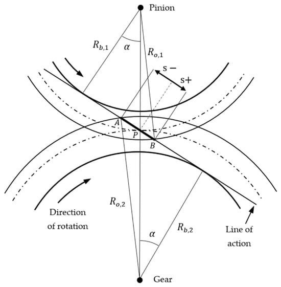
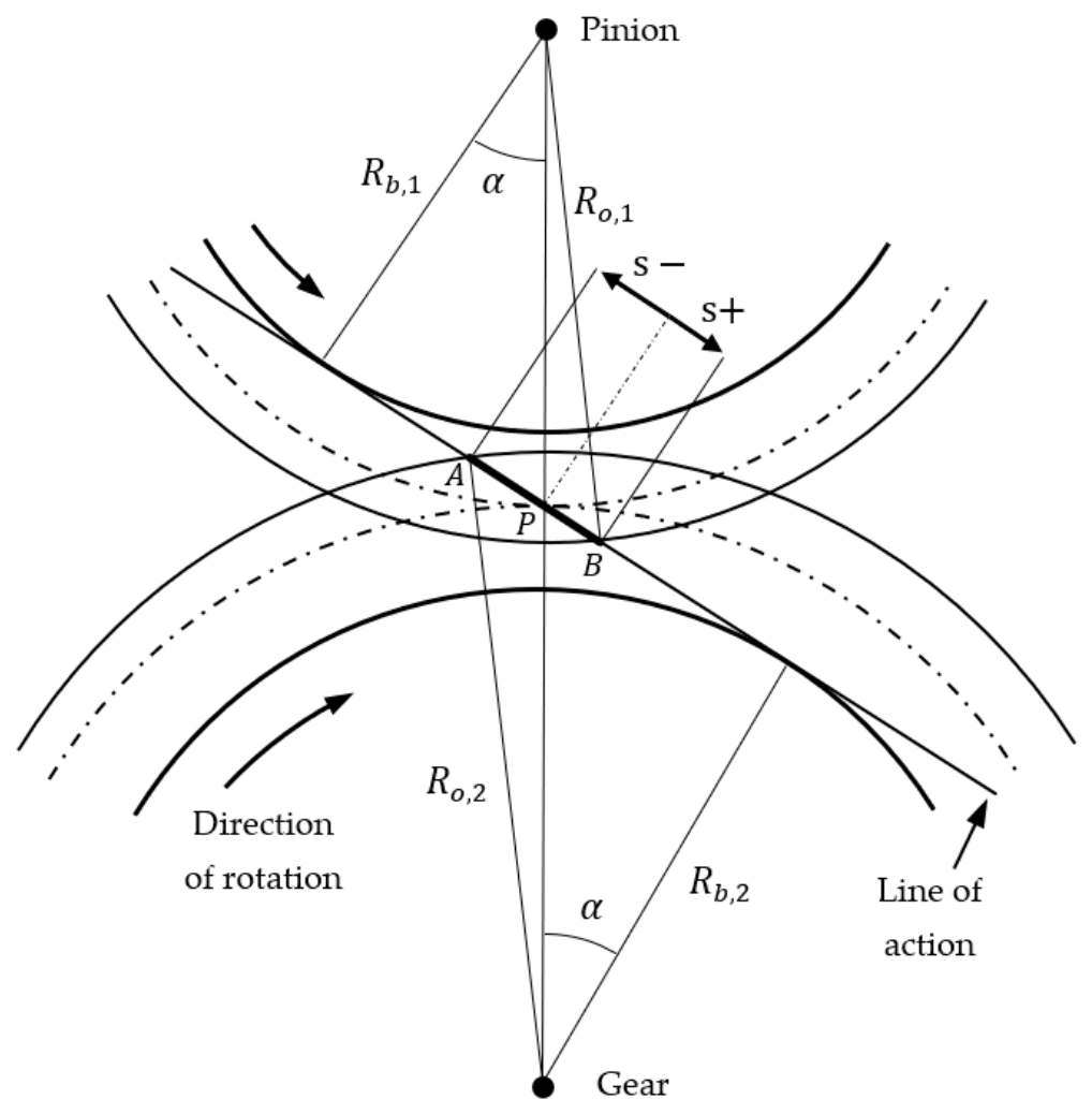
Figure 1 shows the spur gear mesh scheme employed in this work. The gear mesh contact is defined with as the distance along the line of contact from the pitch point. The line of action is tangent to both base circles (of radii and ). The contact begins where the outer radius of the gear () intersects the line of action at point , passes through the pitch point and ends at point where the outer radius of the pinion () intersects the line of action. The pressure angle is the angle between the tooth centreline and the tangent point of the line of action on the base circle.
Figure 1.
Schematic of spur gear meshing adapted from Townsend [31]. The dash-dotted lines represent the pitch circles of the meshing gear pairs.
For a spur gear pair, the normal contact force always acts along the line of action that is at a tangent to the base circle. The relationship between the normal force and applied torque is, therefore,
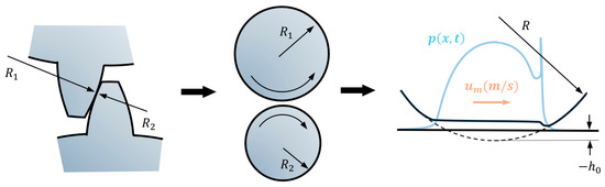
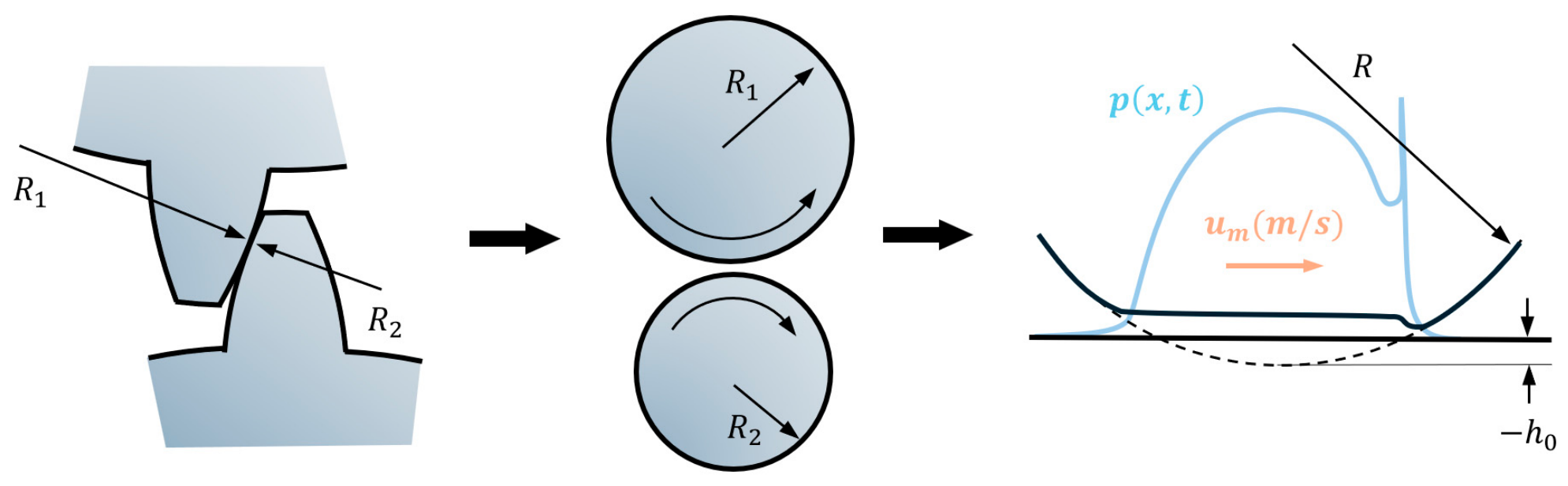
When more than one tooth pair is in contact, the normal force is distributed between the tooth pairs using the load distribution model of Pedrero et al. [32]. The local contact between the meshing teeth is represented as an equivalent EHL line contact with local radii of curvature of and which can be reduced to a single radius (Figure 2). The normal pressure distribution supports the applied normal load, while the rigid-body separation defines the normal approach of the undeformed tooth surfaces.
Figure 2.
Local EHL line contact representation of spur gear contact. The dashed line represents the undeformed elastic body.
2.2. Numerical EHL Solver
For infinitely long contacting bodies, the non-dimensionalised transient Reynolds equation is given by
where with , and , , , , and are the dimensionless pressure, film thickness, time, spatial coordinate in the direction of entraining motion, density and viscosity, respectively, given by
The maximum Hertzian pressure, , and Hertzian contact half-width, , at reference condition are given by
where is the normal load at reference condition, is the contact length, is the equivalent radius at reference condition given by
and is the equivalent elastic modulus given by
The Reynolds boundary condition is applied such that at the inlet and exit. In addition, considering the Reynolds cavitation boundary conditions, the pressure gradient is also set to be equal to zero at the contact outlet. The inlet should be taken as sufficiently large to ensure no numerical/artificial starvation occurs for fully flooded simulations. This is particularly important for low-load and high-speed cases, where inlet lengths of ~100 times the Hertzian half-width may be required.
The dimensionless film thickness equation of Messé and Lubrecht [33] is modified to include the time-varying curvature and load parameters and deformation constant term:
where and are time-varying curvature and load parameters respectively:
and is the additional constant term to fix the datum of the deformation.
is the dimensionless rigid-body separation (or equivalent separation of the undeformed bodies) and can be positive (low-load/high-speed) or negative (high-load/low-speed). Of note here is how the deformation term (including the term) is considered.
The deformation of two cylinders in contact is given by [34]
To determine the value of the constant , Weber’s solution for the Hertzian contact of a gear pair is taken (see Appendix B.1) [3,4]. Wiegert et al. [30] use a similar constant-determination approach but using Johnson’s deformation of cylinders in contact and the approximation of identical bodies (see Appendix B.2). The analysis results in a reference length, , which can be thought of as the point in -direction where deformation is zero for a Hertzian pressure profile loading. The reference length is calculated at every point in the meshing cycle as
where and are distances from the point of contact to the tooth centreline along the line of action of the force. For equal materials, this reduces to
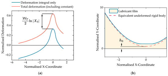
Many prior studies do not consider the contribution of the constant term in the deformation equation. This is acceptable when the only features of interest are film thickness and pressure profiles, since in the associated relaxation procedures, the constant term is absorbed by . However, at this point, no longer represents the exact rigid-body separation, and thus careful consideration must be made when using this approach for stiffness calculations (Figure 3).
Figure 3.
(a) Example deformation in EHL contact showing how the constant raises the deformation such that it is positive throughout the contact. Negative deformations are non-physical. (b) Example film thickness in EHL contact illustrating how the rigid-body separation can be isolated through correct application of the deformation constant.
The elastic deformation integral can be discretised to provide the following relationship for the film thickness:
The coefficients are defined by [35]
This is obtained analytically as
where
and is the grid spacing.
The dimensionless force balance equation is given by
Roelands’ viscosity–pressure relationship [36] and the Dowson and Higginson density–pressure relationship [37] are employed in this investigation and are given as follows, respectively:
where the constants , , and are , , and , respectively [36,37]. The constants and are lubricant density and dynamic viscosity at atmospheric pressure and reference temperatures (usually at 15.6 °C for density and at 40 and 100 °C for viscosity). It is noted here that the reference lubricant density has no impact on the solution. The Roelands’ piezo-viscosity index, , can be found from
where is the lubricant’s piezo-viscosity coefficient.
The governing equations are solved using a multigrid coarse grid correction cycle algorithm with a hybrid Gauss-Seidel and Jacobi dipole relaxation scheme to ensure a fast and stable solution [38,39]. A discrete convolution and FFT (DC-FFT) method similar to that of Liu et al. [40] was used for fast calculation of deformation. Domain sizes were suitably chosen to avoid numerical starvation and grid resolution. Relaxation parameters were also tuned to ensure satisfactory convergence on the finest grid. Convergence is ascertained using the discretisation error for pressure and force balance:
where is the fine grid solution and is the next coarsest solution interpolated into the fine grid using , the interpolation operator. Likewise, and are the forces calculated from summated pressures on the finest grid and next coarsest grid respectively. If convergence is not achieved, the relaxation parameters are manually modified. For more detail on the selection of relaxation parameters, multigrid cycle parameters and domain size, refer to established multigrid literature [38,39,41].
2.3. EHL Contact Force Model
Nonlinear dissipative force models are widely used in multibody dynamic systems with dry clearance joints and contact-impact events [42,43,44]. These models usually describe the normal force through solid body indentation, with energy loss represented using hysteretic damping and commonly a coefficient of restitution [45]. While the dissipative models can be adapted to the study of lubricated contacts [46], a more complete representation of the EHL contact force is given by the three-term reduced-order model comprising local tangent quasi-static stiffness term (, apparent damping term () and force offset () [24]. Here, the nonlinear nature of the contact is accounted for through the local tangent extraction at each operating point, such that the stiffness varies with load, speed, curvature and lubrication state. The primary energy loss mechanism is through the squeeze film damping phenomena as opposed to hysteretic damping during impact.
where is the negative of rigid-body approach (). The quantities , and in Equation (22) are operating-point-dependent coefficients extracted from numerical EHL solutions at each mesh position, rather than prescribed constants. Their values vary with instantaneous normal load, entrainment speed and contact curvature. The procedure for determining the three coefficients is detailed in Section 2.4, Section 2.5 and Section 2.6.
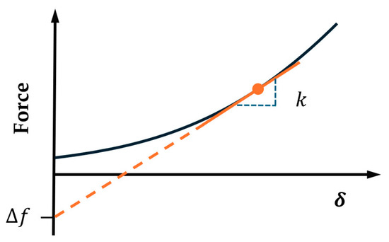
The force offset is the intercept of the local force-approach tangent. This corresponds to the value at which the linearised force extrapolates at zero approach (). It is, therefore, better understood as a geometric intercept than a physical force, since it can hold negative values due to the stiffening nature of elastic contacts (Figure 4). Despite this, the linearisation holds accurate provided the force is evaluated near to the operating point.
Figure 4.
Tangent contact stiffness and force offset.
The contact force model in this study only considers the normal force. The lubricated contact would also contribute a tangential force from the viscous and frictional properties of the lubricating oil and the gear teeth surfaces. Inclusion of these effects is beyond the scope of the present study and is proposed as an extension for future work.
2.4. Stiffness Extraction Method
In this study, a quasi-static numerical tangent contact stiffness extraction method is proposed using the stiffness method, which combines the effect of lubricant and elastic body stiffnesses in series. The extraction comprises two stages: a base solve and an increment solve. The quasi-static base solve uses the instantaneous load, speed and radii of curvature to obtain the converged state at time step by satisfying the dimensionless forms of the Reynolds (with squeeze film term set to zero), film thickness and force balance equations:
For the increment solve, the load is raised to and the squeeze film term is again set to zero. Thus, the governing equations are expressed as follows:
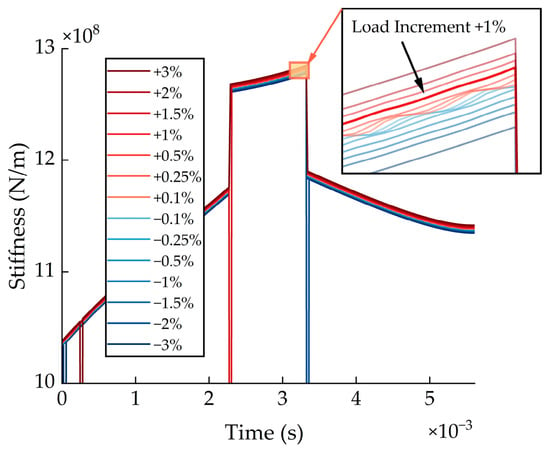
The load increment step must be chosen small enough to ensure linearity but not too small such that noise effects dominate. In this paper, a +1% load increment is used. A load increment sensitivity assessment is included in Section 3.6 to justify the selection of this value.
Stiffness is then extracted by dividing the increment in force by the resultant increment in the rigid-body displacement ():
This provides the quasi-static tangent contact stiffness associated with the lubricant-film and elastic-body compliances, while transient departures from this quasi-static solution are treated separately in the apparent transient residual.
2.5. Force Offset Extraction
Once the stiffness has been calculated, the force offset can simply be extracted using
where is the negative of the quasi-static rigid-body approach ().
2.6. Apparent Transient Damping Extraction Method
The stiffness extraction described in Section 2.4 is performed using the quasi-static Reynolds equation, with the transient squeeze-film term omitted. This provides the instantaneous tangent contact stiffness of the load-controlled EHL contact about the quasi-static operating point. To obtain a corresponding transient force contribution, an additional transient EHL solution is carried out in which the squeeze-film term is retained. This transient base solve uses the instantaneous load, speed, radii of curvature and histories of film thickness and density for the squeeze film term to obtain the converged state at time step by satisfying the dimensionless Reynolds, film thickness and force balance equations:
Now, a transient solution () and a quasi-static solution () at the same imposed load () exist.
The total contact response may be interpreted as the sum of an instantaneous quasi-static contribution and a transient residual contribution:
where denotes the transient EHL residual. In the present work, this residual is represented using an apparent velocity-proportional term (Equation (35)). Methods employed by Fang et al. [21] and Carrer et al. [24] present similar treatments of total force as a steady-stiffness contribution and damping remainder.
It is important to note that should not be interpreted as a pure lubricant-material damping force. It represents the departure of the transient pressure-film solution from the instantaneous quasi-static solution. This departure is expected to be dominated by the squeeze-film contribution in the transient Reynolds equation but may also include effects associated with transient pressure redistribution, coupled elastic deformation response and variation in the quasi-static tangent contact stiffness between the quasi-static and transient rigid-body separations.
The quasi-static force corresponding to the transient rigid-body separation may be written as
where the time dependence denotes the instantaneous operating condition, comprising load, curvature, velocity and lubricant properties. The transient residual force can therefore be expressed as
Direct evaluation of would require an additional quasi-static EHL solution at the transient rigid-body separation. This would increase computational cost and require an EHL solver reformulated in a displacement-controlled form. To retain a load-controlled and computationally efficient extraction framework, is evaluated using a local Taylor expansion about the quasi-static operating point :
Using the quasi-static tangent contact stiffness definition,
and retaining only first-order terms, one can determine as
The neglected second-order term represents the effect of local curvature in the quasi-static force-separation relation, or equivalently, the variation in tangent contact stiffness over the separation excursion between the quasi-static and transient states. This approximation assumes that the quasi-static force-separation relation is locally linear over the small difference .
Since the transient and quasi-static base solutions are obtained at the same imposed load (), the first-order transient residual becomes
Subsequently, the apparent damping coefficient is defined as
where is the time derivative of the transient base trajectory. In order to be consistent with application to gear dynamics simulations, is calculated using the second-order backward finite difference:
The extracted should not be interpreted as a material property of the lubricant or as a unique contact damping constant. It is an apparent coefficient obtained by projecting the transient force residual onto the selected state velocity .
For a quasi-static linearisation check of (Equation (39)), the EHL solver was operated in a fixed- mode, in which the rigid-body separation was prescribed, the force-balance relaxation was disabled, and the resulting quasi-static load was obtained by integrating the converged pressure field, with the deformation datum updated consistently from the generated load at each relaxation step. This yields a direct numerical computation of , which can be compared with the first-order estimate. The results of this linearisation check are presented in Section 3.6.
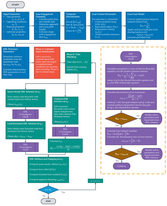
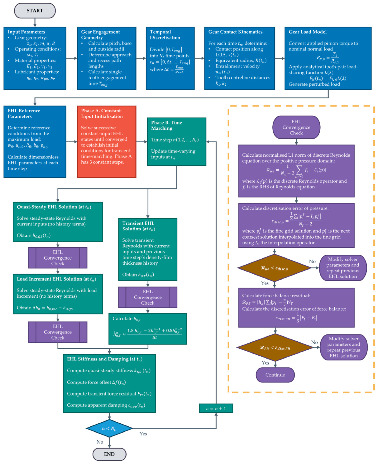
The computational procedure for extracting the stiffness (), apparent damping () and force offset () is detailed in Figure 5.
Figure 5.
Flowchart for stiffness (), apparent damping () and force offset () extraction. The dashed box indicates the ‘EHL Convergence Check’ sub-process which is conducted after each EHL numerical solution.
3. Results and Discussion
3.1. Parameter Inputs
This research investigates the stiffness and damping characteristics of a spur gear pair. Two gear pairs are considered, with gear ratios of 1:1 and 2:1, respectively. The geometry follows that of Blankenship and Kahraman [47], with the remaining relevant parameters taken from Mughal et al. [9] (Table 2 and Table 3).
Table 2.
Gear geometrical and material parameters.
Table 3.
Lubricant properties.
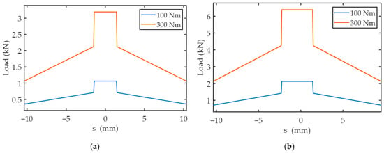
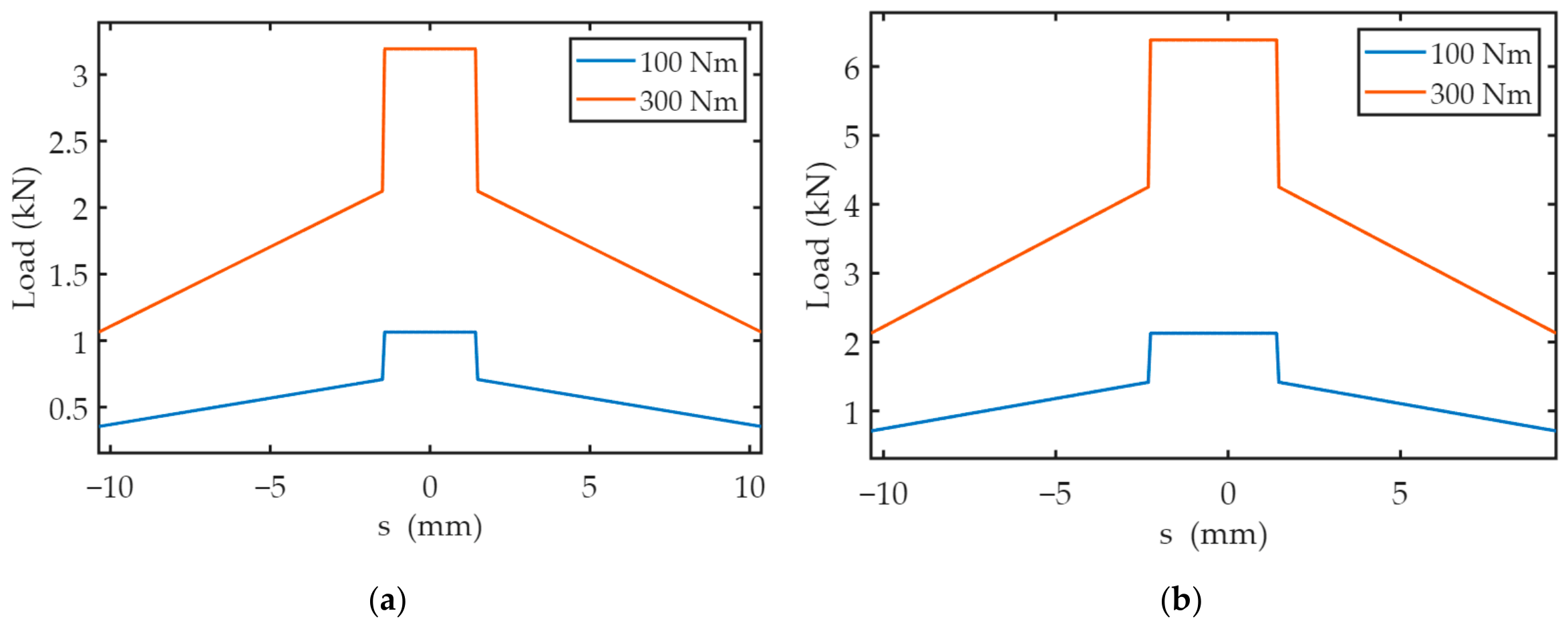
In this work, a single gear mesh cycle is considered, comprising a tooth pair traveling through its full contact. The load distribution model of Pedrero et al. [32] is used to approximate the load share between teeth pairs during meshing, resulting from alternating single and double contact. Figure 6 shows the load distribution profile for gear pairs 1 and 2 for an input torque of 100 Nm and 300 Nm. Here, is the distance along the contact path from the pitch point.
Figure 6.
Load distribution profiles for (a) Gear Pair 1; (b) Gear Pair 2.
This study considers two load-speed combinations (Table 4): 100 Nm at 4200 RPM (low-load/high-speed) and 300 Nm at 720 RPM (high-load/low-speed). Mughal et al. [9] identified these as operating conditions where piezo-viscous rigid and piezo-viscous elastic regimes occur, respectively [17]. The numerical solver parameters must be tuned to ensure there is no artificial starvation due to domain truncation across the whole mesh cycle and that the solution converges to below the discretisation error. A multigrid scheme comprising 7 levels with 1921 nodes on the finest level is used. The mesh cycle is discretised into 300 time steps to strike a balance between computational efficiency and capturing detailed transient physics of the gear contact.
Table 4.
Calculated parameters.
3.2. EHL Contact Stiffness
Based on Weber’s relationship for deformation [3], Equation (43) is derived in this study to provide the closed-form tangent Weber local elastic (Hertzian) stiffness for identical materials:
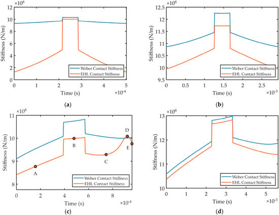
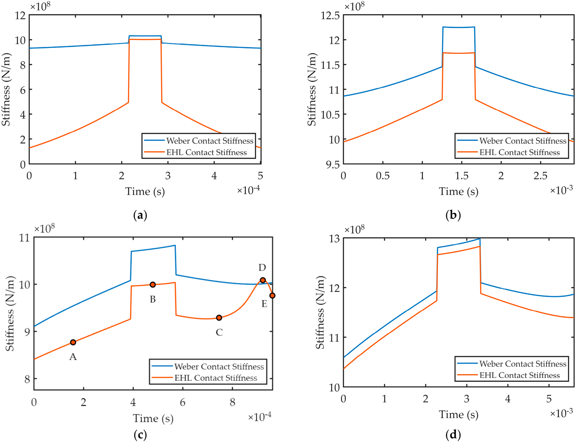
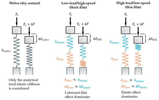
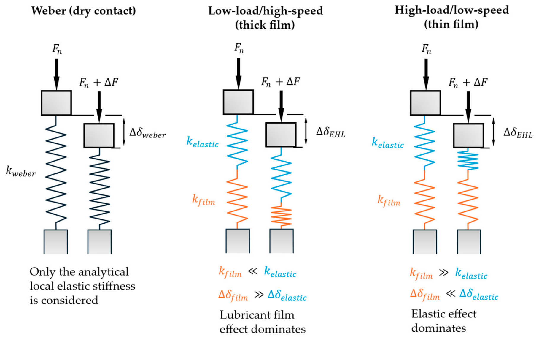
Figure 7 compares the EHL contact stiffness with the Weber local elastic stiffness for both gear pairs and operating conditions. The difference between Weber’s local elastic and EHL stiffness model predictions is the highest for the Gear Pair 1 operating under low-load and high-speed conditions (Figure 7a), while the predictions from both models converge in the case of Gear Pair 2 operating under high-load, low-speed conditions (Figure 7d). This correlates with the maximum Hertzian contact pressures in each case since the former has the lowest whilst the latter has the highest maximum Hertzian pressure (Table 4). At high load and low speed, corresponding to high Moe’s M, the lubricant film thickness in the contact becomes largely invariant to changes in load, and thus the lubricant film stiffness is high. The elastic deformation changes are more appreciable than lubricant film changes, and thus the elastic stiffness dominates in series and the combined EHL contact stiffness tends towards the Weber value. Conversely, at a lower load and higher speed, the lubricant film becomes more compliant, and the EHL stiffness subsequently deviates from the elastic stiffness. Here, the lubricant film is more sensitive to load, and it deforms more significantly compared to the elastic deformation upon load perturbation. Since the film compliance acts in series with the elastic compliance, the total EHL contact stiffness decreases and deviates from the Weber dry contact stiffness. This is illustrated in Figure 8. Two intermediate cases, Gear Pair 1 at high load, low speed (Figure 7b) and Gear Pair 2 at low load, high speed, show notable but comparable deviations. This is consistent with their comparable maximum Hertzian contact pressures (0.5 and 0.6 GPa, respectively).
Figure 7.
Quasi-static EHL contact stiffness and Weber contact stiffness for (a) Gear Pair 1 at 100 Nm and 4200 RPM; (b) Gear Pair 1 at 300 Nm and 720 RPM; (c) Gear Pair 2 at 100 Nm and 4200 RPM (points A-E are mesh locations of interest); (d) Gear Pair 2 at 300Nm and 720 RPM.
Figure 8.
Conceptual series compliance representation of local gear contact stiffness in dry contact conditions, which is represented by a single analytical stiffness, and lubricated contact conditions with elastic and film stiffnesses in series. The EHL stiffness extracted in the present study is the series sum of elastic and film stiffnesses (Appendix A).
This deviation is of practical importance in gear dynamics models, where EHL contact stiffness acts in series with the structural tooth stiffnesses. Since the softest element dominates in series stiffnesses, the lubricant is expected to dominate the mesh behaviour at low-load and high-speed conditions. Representing the contact by its dry elastic stiffness alone would therefore overpredict the mesh stiffness in these conditions, altering the predicted dynamic response.
The elastic (Weber) stiffness provides the equivalent dry contact stiffness. For the unity gear ratio (Gear Pair 1—Figure 7a,b), the stiffness profile is symmetric about the pitch point. The higher load case gives a higher stiffness, highlighting the nonlinear (load-dependent) nature of contact stiffness. For a non-unity gear ratio (Gear Pair 2—Figure 7c,d), asymmetry in the stiffness profile occurs, due to the unequal contributions of reference depths, and , and asymmetric variation in contact half-width, , along the line of contact. The gear ratio thus affects the elastic stiffness through both variations in the load and geometry through the meshing cycle.
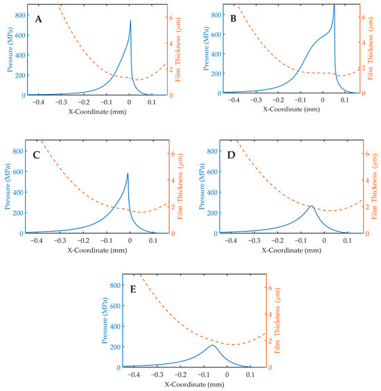
An interesting feature presents itself in Figure 7c, where the EHL contact stiffness rises above the Weber elastic stiffness. This coincides with the contact transitioning out of the typical piezo-viscous-elastic EHL regime, as shown by the quasi-static film thickness and pressure profiles in Figure 9A–D. As the load decreases, the tall, concentrated pressure distribution and its outlet spike give way to a low, broad pressure hump, and the flat, elastically deformed film is replaced by a smooth, almost undeformed one. The feature represents a shift from deformation-dominated to film-dominated load response across the transition between lubrication regimes. This highlights the necessity of applying numerical methods to capture the true physics of EHL contact stiffness in different lubrication regimes and in the transition between lubrication regimes.
Figure 9.
Steady-state pressure and film thickness profiles for mesh locations (A–E) for Gear Pair 2 at low-load/high-speed operating conditions (100 Nm and 4200 RPM).
3.3. Apparent EHL Contact Damping
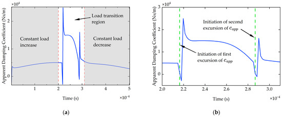
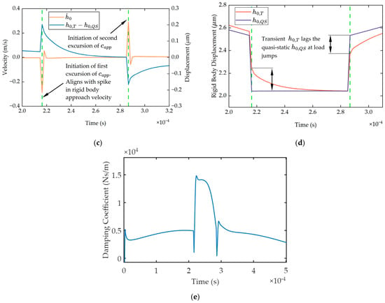
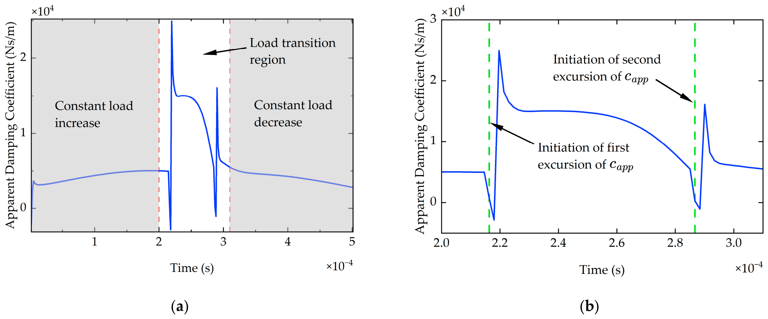
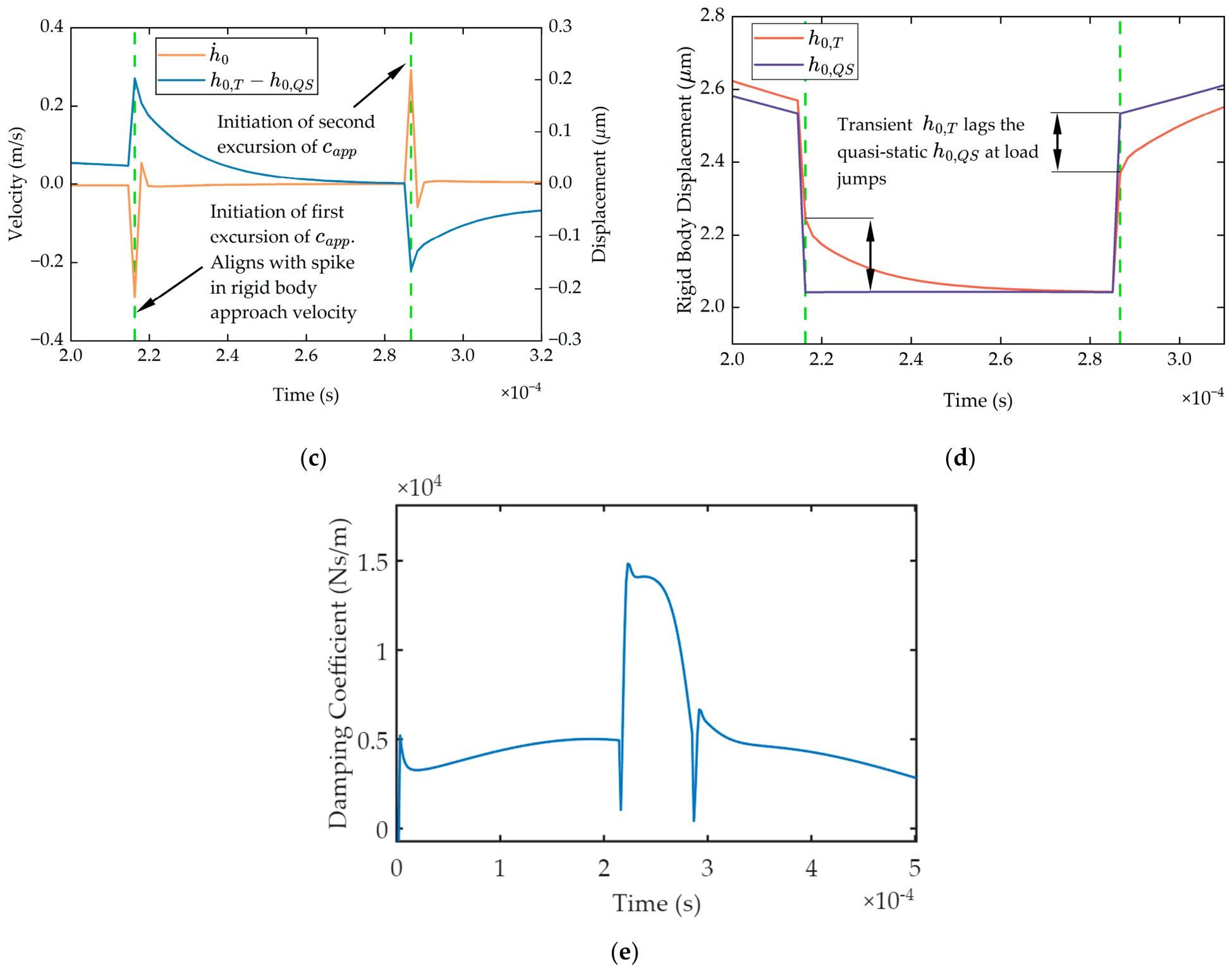
Figure 10a shows the extracted EHL contact damping for Gear Pair 1 (50:50) at 100 Nm and 4200 RPM. Two distinct features produce sharp excursions in the damping coefficient, arising from different mechanisms. The first occurs at the load transitions and can be seen in Figure 10b–d. Here, the imposed load changes abruptly and results in a large (in magnitude) rigid-body approach velocity (). Figure 10b shows a zoomed-in plot of the damping coefficient, with vertical lines plotted at the point when the damping first departs from the smooth section (i.e., after the load jumps) for comparison purposes. Figure 10c confirms that these departures directly correspond to spikes in rigid-body velocity, . At the instant of the jump, the large velocity drives the damping coefficient toward zero. The trailing positive spikes following the abrupt change in are attributed to the use of second-order backwards finite difference for the velocity, which is poorly conditioned for the near-discontinuous change in at the jump and over-represents the resulting velocity transient. Figure 10e shows the apparent damping coefficient extracted using the first-order backwards difference, in which the trailing positive spikes are markedly reduced while the dip at the load transition remains. The second-order backward finite difference scheme is retained throughout this study for consistency with the backward-difference discretisation of the squeeze-film term in Reynolds’ equation and because it is the more appropriate choice for the smoothly varying loading of a live dynamic simulation.
Figure 10.
Gear Pair 1 at 100 Nm and 4200 RPM: (a) Apparent damping coefficient across whole mesh cycle; (b) apparent damping coefficient across central part of mesh cycle; (c) rigid-body velocity () and difference in transient and quasi-static rigid-body displacements () across central part of meshing cycle; (d) transient rigid-body displacement () and quasi-static rigid-body displacement () across central part of meshing cycle; (e) apparent damping coefficient across whole mesh cycle calculated using first-order backward difference for rigid-body velocity in Equation (42).
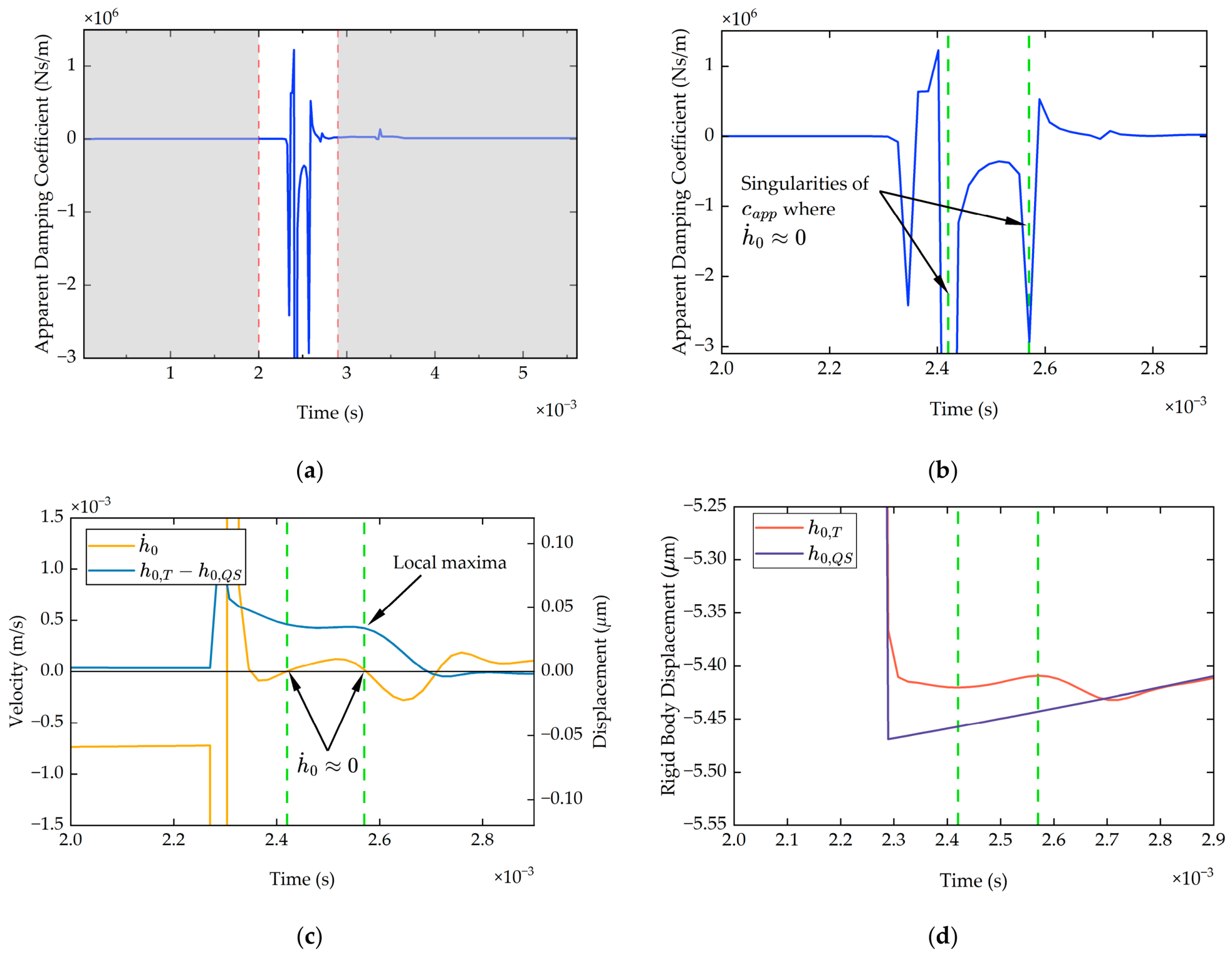
The second feature arises from the transient response to the prescribed step change in load. Following each step, the rigid-body approach overshoots and relaxes towards the quasi-static value. At the turning points of , the rigid-body velocity is zero (), and the difference in transient and quasi-static rigid-body displacement is near a local maximum; thus, the transient residual force does not vanish. Therefore, this results in a series of singularities in the damping coefficient, one at each velocity reversal of the relaxing transient, which are intrinsic to the definition of a velocity-proportional coefficient (i.e., undefined at ). Figure 11a,b show the damping coefficient for Gear Pair 2 (25:50) at 300 Nm and 720 RPM. Two singularities are highlighted by vertical lines, and it can be seen in Figure 11c,d that these correspond to the rigid-body velocity reversal points and where experiences a local maximum.
Figure 11.
Gear Pair 2 at 300 Nm and 720 RPM: (a) apparent damping coefficient across whole mesh cycle; (b) apparent damping coefficient across central part of mesh cycle; (c) rigid-body velocity () and difference in transient and quasi-static rigid-body displacements () across central part of meshing cycle; (d) transient rigid-body displacement () and quasi-static rigid-body displacement () across central part of meshing cycle.
Figure 11a,b also show that the extracted damping coefficient becomes negative over part of the mesh cycle. This occurs when and hold the same sign. A negative value cannot represent squeeze-film dissipation and is attributed here to the state used in the extraction. The energy-loss mechanism of squeeze-film damping is governed by the rate of change in the lubricant film thickness, whereas the present extraction method relates damping to the rigid-body approach , which combines both film and elastic-deformation contributions. The rate therefore does not map directly onto the film-thickness rate to which analytical squeeze-damping formulations [48,49] are referred. It is hypothesised that, during the post-jump relaxation, the lubricant film and deformation contributions to evolve out of step (deformation is near-instantaneous, film is lagged), so that the inferred transient residual force is no longer proportional to directly and a negative apparent coefficient results. This interrelationship is complex and would be difficult to assess fully, owing to the difficulty of separating the lubricant-film and deformation contributions to , the same obstacle noted for stiffness-extraction methods reviewed in the introduction. This does not compromise use of the extracted damping coefficient, however. The transient EHL residual force remains bounded and continuous through both the velocity reversals and the negative-coefficient regions, and it is this product, not the coefficient in isolation, that enters the reconstructed force. The features described above are present in the extracted damping coefficients for both gear pairs under both operating conditions; the complete set is provided in Appendix C.
3.4. Contact Force Reconstruction
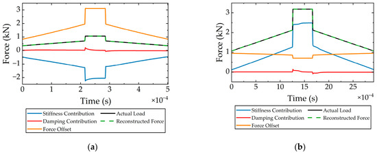
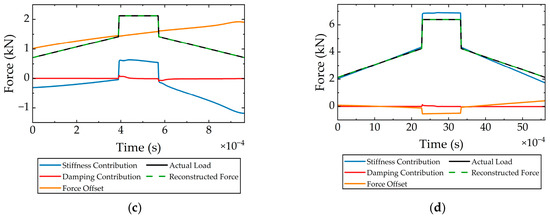
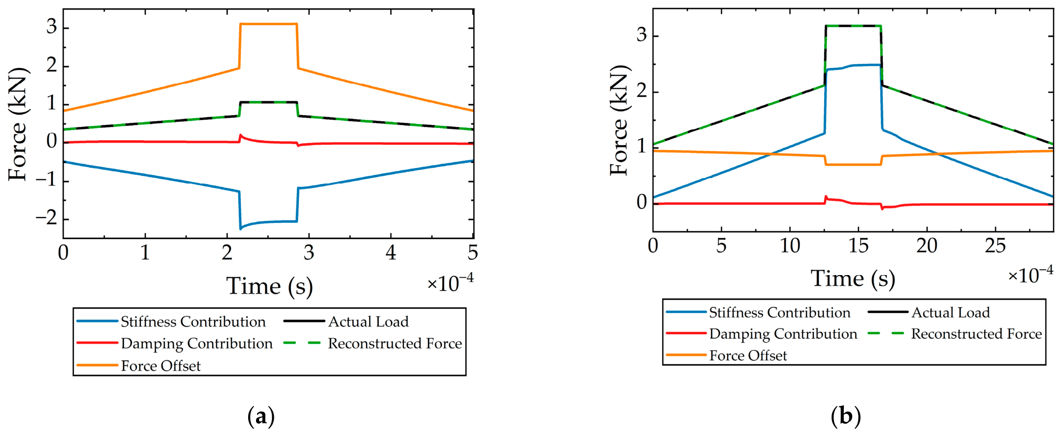
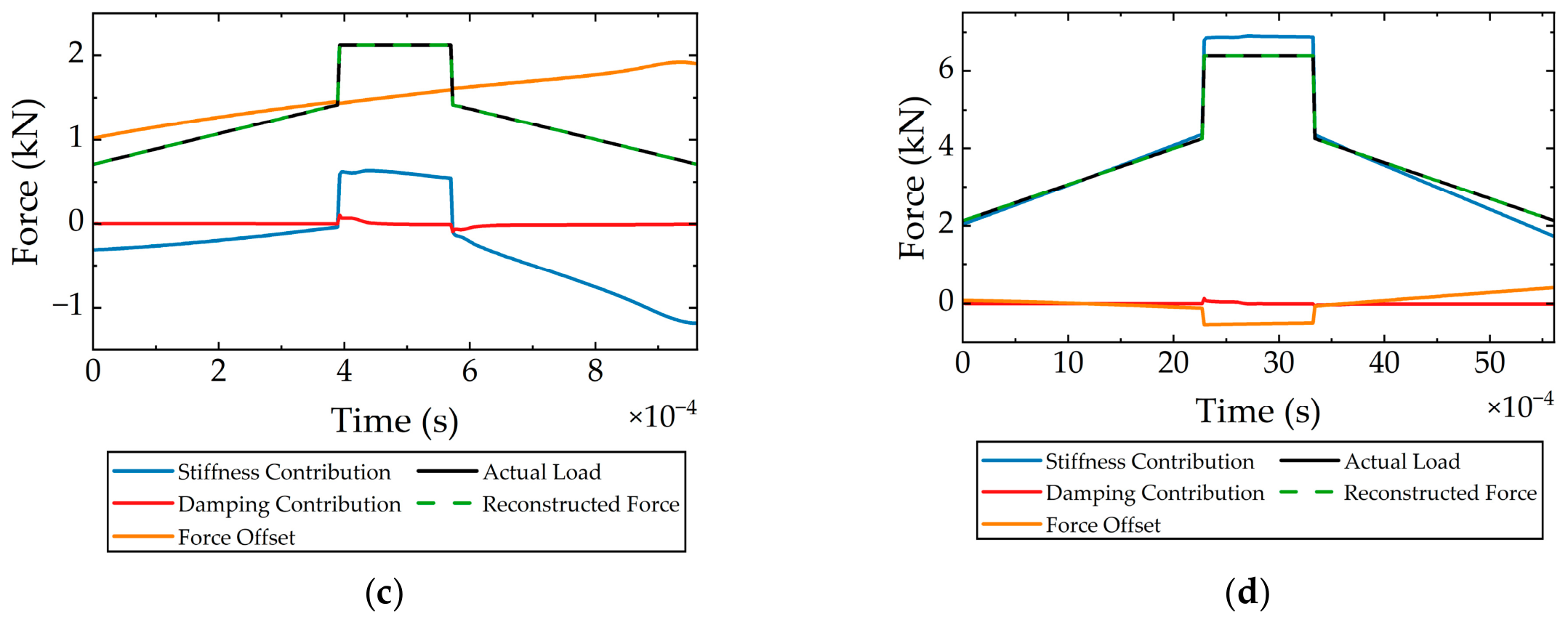
The EHL contact force is reconstructed using the extracted stiffness, damping coefficient and force offset alongside the state variables and (Figure 12). Importantly, the discontinuities in the damping coefficient have no effect on the reconstructed force. The physically meaningful quantity is the transient force residual (), which remains bounded and smooth through the velocity reversals. The damping force remains of small magnitude across the mesh cycle, with variations at the load jumps, as expected. The stiffness contribution largely follows the trend of the rigid-body approach, since they are directly multiplied except when the change in stiffness outweighs the trend in rigid-body approach (Figure 12a).
Figure 12.
Reconstructed EHL contact force, actual contact force, stiffness contribution, damping contribution and force offset for (a) Gear Pair 1 at 100 Nm and 4200 RPM; (b) Gear Pair 1 at 300 Nm and 720 RPM; (c) Gear Pair 2 at 100 Nm and 4200 RPM; (d) Gear Pair 2 at 300Nm and 720 RPM.
The force offset term is positive across the mesh cycle in Figure 12a–c but is negative for part of the meshing cycle, as shown in Figure 12d. This is ascribed to the aforementioned local tangent linearisation. The force offset should be interpreted as the intercept of the local tangent force–approach relationship. Since the EHL contact response is nonlinear, the local tangent line does not pass through the origin. The offset is required such that the reduced-order linear representation passes through the quasi-static operating point. The stiffening nature of the EHL contact at a higher load steepens the tangent, lowering the zero-approach intercept, and resulting in a negative force offset.
The discontinuous features in the apparent damping coefficient may have an impact on the numerical stability of practical gear dynamic simulations. The present study has not implemented integration of the proposed approach with dynamics; however, a few comments can be made. In an implicit scheme such as Newmark-, the damping coefficient contributes to the effective dynamic stiffness. Very large or rapidly varying values of near rigid-body velocity reversals may therefore introduce numerical stiffness, poor conditioning and potential numerical instability. A sufficiently small timestep should be used to capture the smooth evolution of displacement, velocity and dynamic mesh force across the mesh cycle. The raw apparent damping coefficient may remain ill-conditioned near velocity reversals. For practical implementation, smoothing, limiting or velocity regularisation of may therefore be required.
3.5. Load Increment Sensitivity
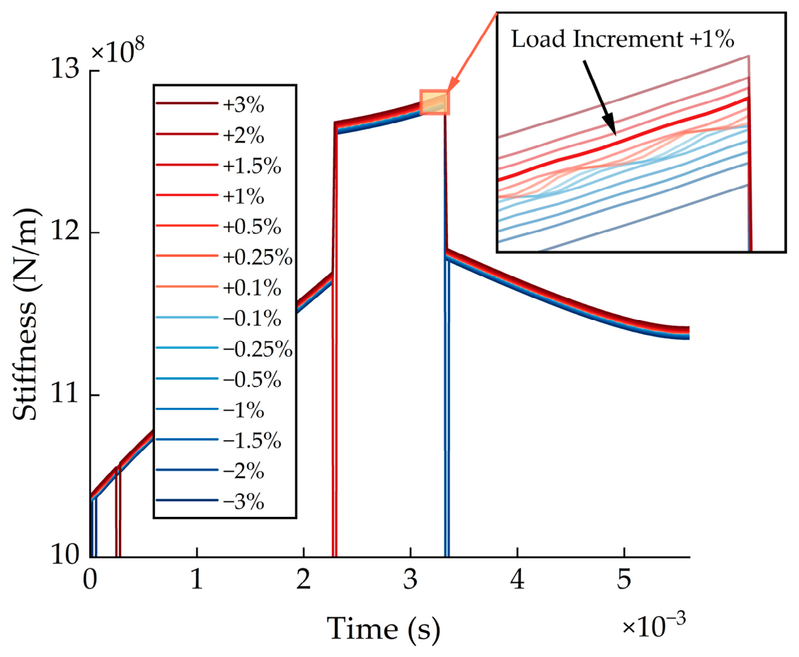
The stiffness extraction method presented in this study requires a load perturbation to approximate the local tangent contact stiffness. The increment in load must be sufficiently small to represent the local force-separation gradient but sufficiently large that the resulting change in rigid-body separation is not dominated by numerical noise. The sensitivity study for Gear Pair 2 at 300 Nm and 720 RPM is presented here, since it produces the largest contact stiffness magnitude and is the case most likely to show numerical noise at small load increments. Figure 13 shows the extracted contact stiffness for load increments ranging from −3% to +3%. A load increment of +1% represents a perturbation that is large enough to not produce numerical noise but small enough to approximate the local tangent stiffness to within 0.14% of a central reference obtained from a ±0.005% perturbation. Larger load increments can pose issues with numerical instability of the EHL solver. The same 1% load increment was therefore used for both gear pairs and operating conditions in the present study.
Figure 13.
Load-increment sensitivity of the extracted quasi-static EHL contact stiffness for Gear Pair 2 at 300 Nm and 720 RPM.
3.6. Quasi-Static Linearisation Check
As detailed in the presented methodology, the EHL solver was operated in a fixed- mode in order to obtain the quasi-static force corresponding directly to the rigid-body separation of the transient case, . This yields a direct quasi-static reference force, , against which the first-order local linear estimate can be tested. The linearisation is considered accurate when
where .
The linearisation error is then defined as
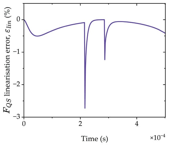
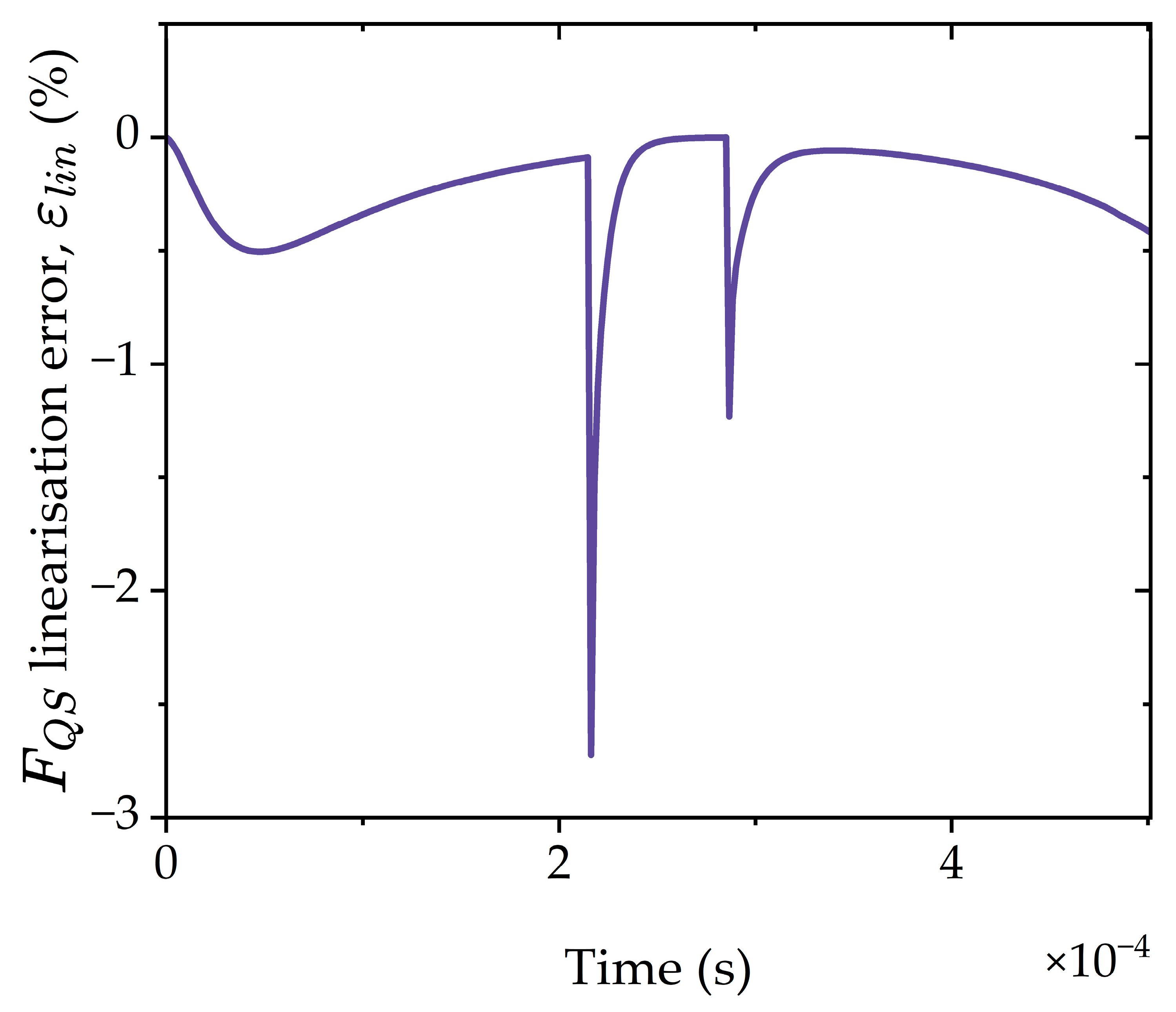
Figure 14 shows the linearisation error across the mesh cycle for Gear Pair 1 at 100 Nm and 4200 RPM. This case was selected because it produced the largest difference between and , and therefore represents the most demanding case for local linearisation. The error remains small (<0.5%) over much of the mesh cycle, indicating that the local tangent approximation gives a close estimate of the quasi-static force at transient rigid-body separation. Larger errors occur near load-transition regions, where the transient separation excursion is largest. Even in these regions, the maximum error remains below 3%.
Figure 14.
Linearisation error across mesh cycle for Gear Pair 1 at 100 Nm and 4200 RPM.
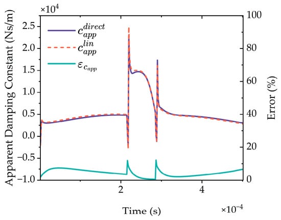
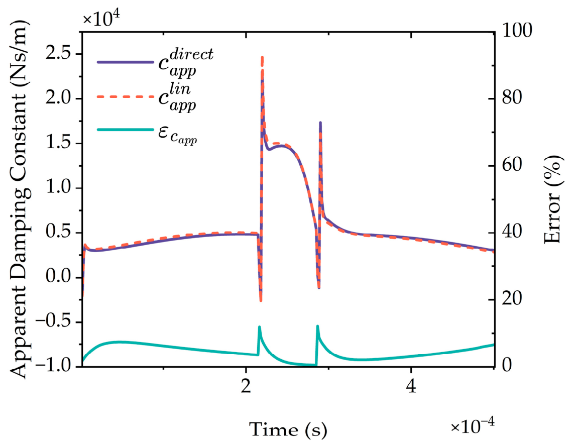
The apparent damping coefficient can be extracted using and compared with the original apparent damping coefficient from linear approximation. The error between the apparent damping coefficient using the direct quasi-static force () and that using the first-order linear approximation () is calculated using
Figure 15 shows that closely follows across the mesh cycle, including the main trends and sharp excursions associated with load transitions. The error remains small over most of the cycle, with the larger local errors occurring near the same transition regions identified in the force linearisation check. This indicates that the first-order approximation captures the dominant behaviour of the apparent damping coefficient. Hence, the first-order method is retained in the present study due to its computational efficiency (one less EHL solution) and the numerical complexity of a fixed- EHL solver while preserving the main apparent damping behaviour.
Figure 15.
Comparison of apparent damping coefficients obtained using the direct quasi-static force evaluation and the first-order local linearisation for Gear Pair 1 at 100 Nm and 4200 RPM. The direct coefficient is calculated from , while is calculated from the tangent approximation .
3.7. Computational Cost
Computational time for the numerical extraction of stiffness and damping using a multigrid solver with 1921 points on the finest grid and 300 time steps per mesh cycle takes between 675 and 1035 s per mesh cycle on a 1.3 GHz Intel Core i5 processor, depending on the gear pair and operating conditions selected. This timing includes the quasi-static base, quasi-static load increment and transient EHL solutions required at each time step for the proposed extraction method (Figure 5).
4. Conclusions
This work presents a perturbation-based extraction method for gear contact stiffness, apparent damping and force offset terms including lubricant film effects for future application to gear dynamics studies. From the results, the following conclusions can be drawn:
- (1)
- The lubricated contact stiffness is obtained from the rigid-body separation, combining the film and elastic compliances in series through a deformation datum defined from Weber’s local elastic deformation of the gear teeth. This resolves the inconsistent datum treatments in existing rigid-body displacement methods.
- (2)
- The lubricated contact stiffness tends towards the closed-form Weber local elastic stiffness at high loads where lubricant film is very stiff and contributes negligibly to the series sum of film and elastic stiffnesses.
- (3)
- At low loads, the EHL contact stiffness deviates from the Weber contact stiffness by up to an order of magnitude for the conditions tested in the present study. This is expected to affect the TVMS in gear dynamic models and, consequently, the predicted noise and vibration response.
- (4)
- The transient EHL residual force is extracted from a local linearisation of the stiffness force across the difference between the quasi-static base solution and the transient solution. The extracted apparent damping coefficient exhibits singularities at rigid-body velocity reversals, reflecting the definition of a velocity-proportional constant and use of rigid-body approach as the reference state. The transient EHL residual force remains bounded across the mesh cycle.
- (5)
- The extracted force offset represents a geometric intercept of the local force-approach tangent and does not reflect a physical force at zero approach. It may take a negative value at a high load where a steeper tangent intercepts below zero.
- (6)
- The stiffness linearisation across the transient separation excursion is validated directly against fixed-separation EHL solutions with agreement to within 3%. While this has a minor effect on the apparent damping coefficient, the linearised method is retained as it reduces computational cost and complexity.
- (7)
- Force reconstruction confirms recovery of the full transient contact force across the mesh cycle. This highlights the method’s application potential to spur gear dynamic models.
Some limitations of the proposed approach are noted:
- (1)
- The stiffness extraction is based on a first-order local linearisation of the quasi-static force-separation response about the instantaneous operating point. Higher-order approximations may provide more accurate results but would be more computationally expensive.
- (2)
- It is assumed that EHL contact stiffness is a quasi-static coefficient. All transient effects are contained within the transient force residual.
- (3)
- It is assumed that the transient force residual is dominated by squeeze film effects. The extracted apparent damping coefficient is a state-dependent coefficient rather than a unique material or lubricant property.
- (4)
- The present model is restricted to the normal EHL contact response.
The principal direction for future work is the development of a fully coupled tribodynamic model, applying the numerically extracted stiffness, apparent damping and force offset within the equations of motion. EHL contact stiffness would be combined in series with structural tooth stiffness formulations. This would enable the assessment of lubricant effects on vibrational characteristics and their nonlinearity and offer validation against experimental datasets. A wider parametric study could be completed to fully assess the impact of changing operational conditions and gear geometry on the extracted coefficients. Finally, the model could be extended to include additional phenomena such as tangential friction, thermal and mixed lubrication effects.
The significance of this work is in bridging the gap between high-fidelity tribological numerical modelling and reduced-order gear dynamic analysis. These fields have remained largely separate because of a persistent narrative of high computational cost associated with EHL numerical modelling. The study has shown that this is not necessarily the case and that it is possible to extract operating-point-dependent stiffness and apparent damping coefficients efficiently, providing an approach for lubricant film effects to be incorporated into gear dynamics workflows. Quantification of the computational cost in coupled system-level simulations remains a subject of future work. The finding that the lubricant film deviates from dry contact stiffness under low-load, high-speed conditions has a direct impact for engineering practice, particularly in the assessment of electric vehicle (EV) gear trains in which these conditions are prevalent. As such, modelling methods currently in use in industry may misrepresent the dynamic response in the operating regimes most relevant to high-speed EV transmissions. The approach presented here, therefore, offers a route to account for the lubricant effect in gear noise and vibration prediction, supporting the development of quieter and more efficient transmissions.
Author Contributions
Conceptualisation, T.C., N.D. and R.R.; methodology, T.C., N.D. and R.R.; software, T.C.; validation, T.C.; formal analysis, T.C.; investigation, T.C.; resources, R.R.; data curation, T.C.; writing—original draft preparation, T.C.; writing—review and editing, T.C., N.D. and R.R.; visualisation, T.C.; supervision, N.D. and R.R.; project administration, R.R.; funding acquisition, T.C. and R.R. All authors have read and agreed to the published version of the manuscript.
Funding
This research received no external funding.
Data Availability Statement
Data will be made available upon request.
Acknowledgments
The authors gratefully acknowledge the financial support of the Vice Chancellor’s Academic Excellence Scholarship, which funded the Ph.D. studentship of Tom Caston. During the preparation of this manuscript, Claude Opus 4.8 (Anthropic) was used to improve the language and readability of drafted text. The authors have reviewed and edited the output and take full responsibility for the content of this publication.
Conflicts of Interest
The authors declare no conflicts of interest.
Nomenclature
| Roman symbols | |
| Contact length/gear face width (m) | |
| Hertzian contact halfwidth (m) | |
| Constant in elastic deformation expression (m) | |
| Modified deformation constant (m) | |
| Dowson–Higginson density coefficients (Pa−1) | |
| Apparent damping coefficient obtained by projecting the transient residual force onto rigid-body approach velocity (Ns/m) | |
| Grid spacing in dimensionless coordinate | |
| Young’s Modulus of Elasticity (Pa) | |
| Equivalent elastic modulus ((Pa) | |
| Reduced elastic modulus ((Pa) | |
| Palmgren’s equivalent modulus (Pa) | |
| Normal contact force (N) | |
| Reference normal load (N) | |
| Total EHL force (N) | |
| Applied load (N) | |
| Quasi-static force (N) | |
| Apparent transient EHL residual force (N) | |
| Transient force (N) | |
| Nodal force (N) | |
| Force offset (N) | |
| Dimensionless curvature parameter | |
| Geometrical term in film thickness (m) | |
| Dimensionless film thickness | |
| Dimensionless rigid-body separation | |
| Film thickness (m) | |
| Rigid-body separation (m) | |
| Central film thickness (m) | |
| Nodal film thickness (m) | |
| Discrete deformation kernel coefficient | |
| Generic contact stiffness (N/m) | |
| Elastic stiffness (N/m) | |
| Film stiffness (N/m) | |
| Rigid-body displacement (total equivalent) stiffness (N/m) | |
| Tangent contact stiffness (N/m) | |
| Average contact stiffness (N/m) | |
| Quasi-static local tangent EHL contact stiffness (N/m) | |
| Reference depths for gears teeth 1 and 2 measured as distance from point of contact to tooth centreline along the line of action of the contact force (m) | |
| Moe’s Dimensionless Parameter | |
| Moe’s Dimensionless Parameter | |
| Gear module | |
| Number of nodes | |
| Dimensionless pressure | |
| Pressure (Pa) | |
| Maximum Hertzian pressure (Pa) | |
| Reference maximum Hertzian pressure (Pa) | |
| Roeland’s reference pressure (Pa) | |
| Equivalent radius of curvature (m) | |
| Reference equivalent radius (m) | |
| Principal radii of curvature of contacting gear teeth (m) | |
| Elastically-weighted geometric mean radius (m) | |
| Distance along the line of contact from pitch point (m) | |
| Dimensionless time | |
| Time (s) | |
| Dimensionless speed parameter | |
| Mean entrainment speed (m/s) | |
| Half-plane displacement from logarithmic kernel with zero arbitrary constant (m) | |
| Elastic deformation term in film thickness (m) | |
| Dimensionless load parameter | |
| Dimensionless spatial coordinate in direction of entraining motion | |
| Dimensionless deformation reference length | |
| Dimensionless nodal coordinates | |
| Auxiliary kernel variables | |
| Spatial coordinate in direction of entraining motion (m) | |
| Deformation reference length (m) | |
| Roeland’s pressure-viscosity index | |
| Number of gear teeth | |
| Greek symbols | |
| Pressure angle (rad or ) | |
| Piezo-viscosity coefficient (Pa−1) | |
| Rigid-body approach (m) () In Appendix B only, denotes local dry-contact elastic deformation in the cited Weber, Palmgren and Johnson formulae | |
| Approach velocity (m/s) | |
| Weber deformation (m) | |
| Increment/change operator | |
| Quasi-static force linearisation error (%) | |
| Apparent damping coefficient error (%) | |
| Pressure discretisation error | |
| Force-balance discretisation error | |
| Dynamic viscosity (Pa s) | |
| Reference viscosity | |
| Roeland’s reference viscosity | |
| Dimensionless parameter in Reynolds equation | |
| Poisson’s ratio | |
| Poisson’s ratio of contacting bodies | |
| Coefficient in Reynolds equation | |
| Density | |
| Reference density | |
| Integration domain | |
| Subscripts/Superscripts | |
| Apparent | |
| Average | |
| Direct fixed- quasi-static evaluation | |
| Central | |
| Elastic | |
| Elastohydrodynamic | |
| Film | |
| Geometric | |
| Global | |
| Hertzian | |
| Node indices | |
| Incremented solution | |
| First-order linearised estimate | |
| Local/tangent | |
| Current timestep | |
| Plus/minus auxiliary indices | |
| Quasi-static | |
| Transient residual | |
| Transient | |
| Weber | |
| Reference condition | |
| Abbreviations | |
| EHL | Elastohydrodynamic lubrication |
| EV | Electric eehicle |
| FEM | Finite element method |
| TVMD | Time-varying mesh damping |
| TVMS | Time-varying mesh stiffness |
Appendix A
The series combination of separately extracted EHL film stiffness, , and elastic stiffness, , are identically equal to the rigid-body displacement stiffness, :
The (simplified) film thickness equation reads
where is the rigid-body displacement, is the geometrical term and is the local elastic deformation of the solid surfaces. A load increment results in a change in the rigid-body displacement, , a change in film thickness, , and a change in elastic deformation, . This results in an expression for the change in film thickness:
Appendix A.1. Global Method
The global method treats the contact zone as a discrete network of parallel springs distributed across individual nodes . At any node , the local force increment is , where the total load increment is the sum of the nodal increments: . At each node, the film thickness relation holds:
Dividing by the local nodal force increment yields nodal compliance (inverse of stiffness):
Rearranging leads to
Taking the sum across the domain results in
which can be expressed as
Thus, the series sum of the film and elastic components is equal to the equivalent stiffness using rigid-body displacement. This is a tangent stiffness.
Appendix A.2. Average Method
Integrating the film thickness equation across the domain, , yields
Since is a uniform rigid-body shift and independent of , its average is simply itself:
Dividing by the total force increment yields the compliances:
This can be expressed in terms of stiffnesses as
Therefore,
Again, the series sum of the film and elastic components is equal to the equivalent stiffness using rigid-body displacement.
Appendix A.3. Central Method
From the film thickness expression at the centre of the contact:
Dividing by the force increment gives compliance:
This can be expressed in stiffnesses as
Therefore,
Again, the series sum of the film and elastic components is equal to the equivalent stiffness using rigid-body displacement.
Appendix B
Appendix B.1
A logarithmic Green’s function results in a displacement field whose absolute vertical value is not unique, requiring the specification of a datum or reference condition. Here, the datum is defined by equating the deformation at the centre to that of Weber’s deformation of gear teeth in contact.
The deformation for a line contact is given by
For a line contact, the Hertzian pressure profile is given as
Substituting into the deformation equation gives
Letting and ,
Concerning the deformation at the centre of the contact (i.e., where ),
Evaluating the integral,
Substituting into Equation (A22) gives
which then simplifies to
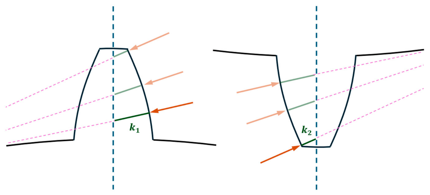
Weber gives the local deformation of two gear teeth in contact as [3]
where and are the distances on the pinion and the gear between the point of contact and the tooth centrelines along the line of action of the force (Figure A1). The approach outlined by Cornell [50] is applied in the calculation of and . The values of and are the reference depths at which the deformation is considered to be zero. For unity gear ratios, and are symmetric across the pitch point, whereas for non-unity gear pairs, asymmetry in and manifests as asymmetry in the deformation, and thus stiffness profiles across the mesh cycle.
Figure A1.
Illustration of the how and vary across the mesh cycle. The arrows represent the normal contact force.
Equating Equations (A25) and (A26) gives: ()
Rearranging for gives
This can be expressed as
where is given by (A13) for unequal materials and (A14) for equal materials:
Appendix B.2
Johnson gives the deformation of two cylinders in contact as
The total deformation is therefore given by
This can then be represented by
where is an elastically weighted geometric mean radius given by
For cylinders of identical materials, this reduces to
Equating the two gives: ()
Rearranging for gives
This can be expressed as
Appendix B.3
Returning to the equation for the deformation of the centre of contact according to the elastic half-space approximation,
If we just consider the half-plane displacement from the logarithmic kernel with zero arbitrary constant as ,
Since , this simplifies to
And can be represented in the form of Tian et al. [22] as
Note that there is an extra term in the equation compared to Tian et al.’s [22] . Therefore, this can be considered as being absorbed into the constant as
where
However, Tian et al. [22] do not account for this extra term in the constant and only account for the term. The remaining logarithmic term ( is not treated explicitly and is therefore absorbed (or remains within ), even after the correction has been applied. Therefore, Tian et al.’s [22] correction factor, obtained by subtracting from Palmgren’s empirical Hertzian deformation, does not by itself fully specify the displacement reference. In Tian et al.’s formulation, must therefore accommodate the remaining offset, even after the correction has been applied. It is thus not consistent with the present paper’s reference choice, in which remains equal to the rigid-body displacement rather than absorbing part of the half-space displacement offset.
Appendix B.4
Here, some common local contact stiffness formulations are provided. The Weber [3,4] and Johnson [51] formulations are based on Hertzian contact theory with different reference depths and stress contributions taken respectively. Palmgren’s approach [26] is empirical. The local (tangent) stiffness for each approach is determined by performing the partial derivative of force with respect to deformation while the average (secant) stiffness is determined simply by division of the force by the deformation.
Appendix B.4.1. Weber
Appendix B.4.2. Palmgren
Appendix B.4.3. Johnson
Appendix C
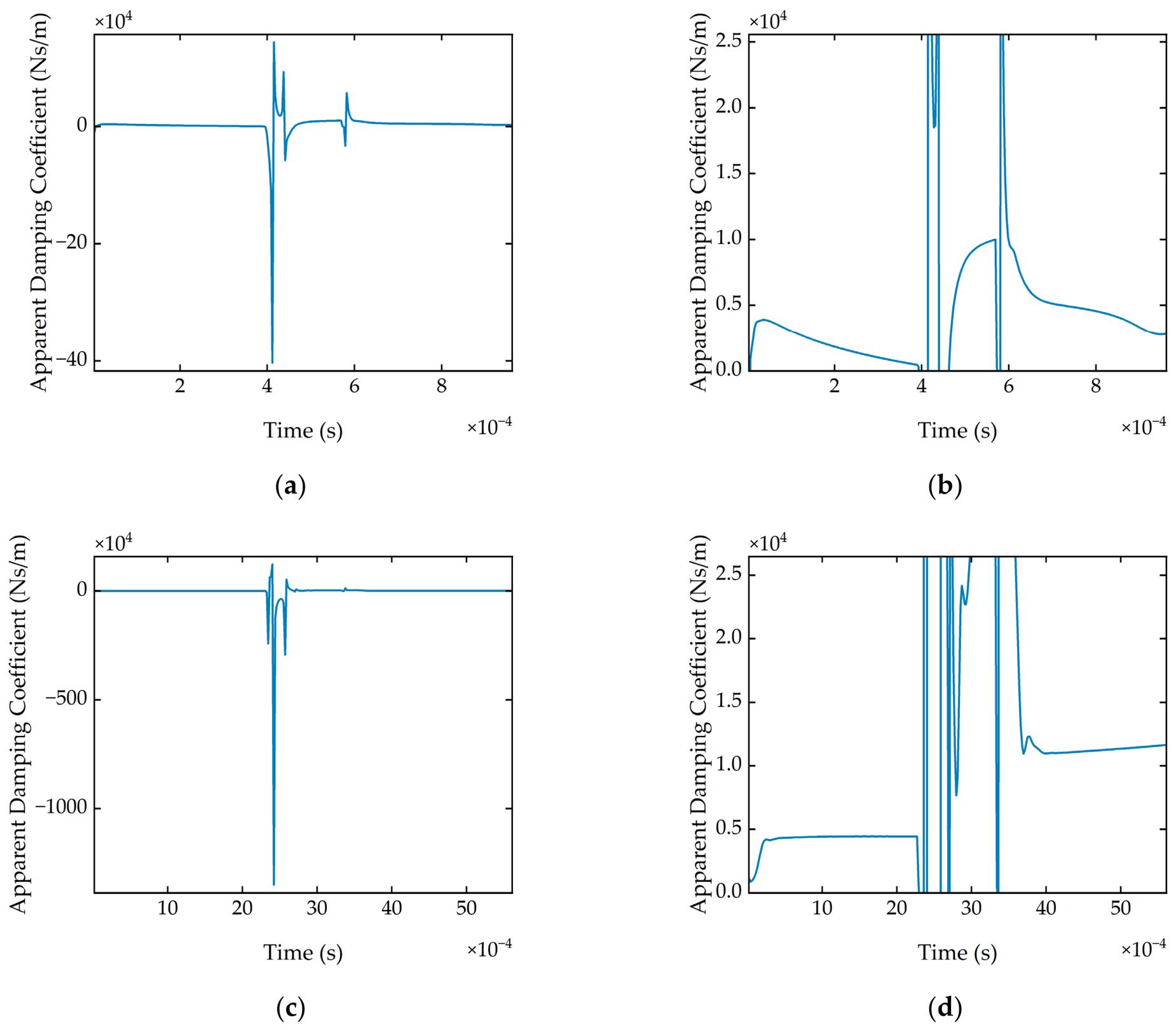
The apparent damping coefficients for Gear Pair 1 (50:50) under both operating conditions are given in Figure A2. The apparent damping coefficients for Gear Pair 2 (25:50) under both operating conditions are given in Figure A3. In Figure A2b,d and Figure A3b,d, the y-axis has been scaled to the same values for comparison. Of note is that the apparent damping coefficient in the period of steady load increase before load step is greater for the higher-load, lower-speed cases than the lower-load, higher-speed cases. This is attributable to the thinner lubricant film in the high-load, low-speed cases, where the higher load and lower entrainment both reduce film thickness. Subsequently, the resistance to squeezing oil from the contact, and hence the damping, increases strongly as the film thins. Although the apparent damping coefficient is extracted with respect to the rigid-body approach rather than the film thickness directly, still carries transient squeeze-film behaviour, so the same trend follows.
Figure A2.
Gear Pair 1 at (a) 100 Nm and 4200 RPM; (b) 100 Nm and 4200 RPM with zoomed y-axis; (c) 300 Nm and 720 RPM; (d) 300 Nm and 720 RPM with zoomed y-axis.
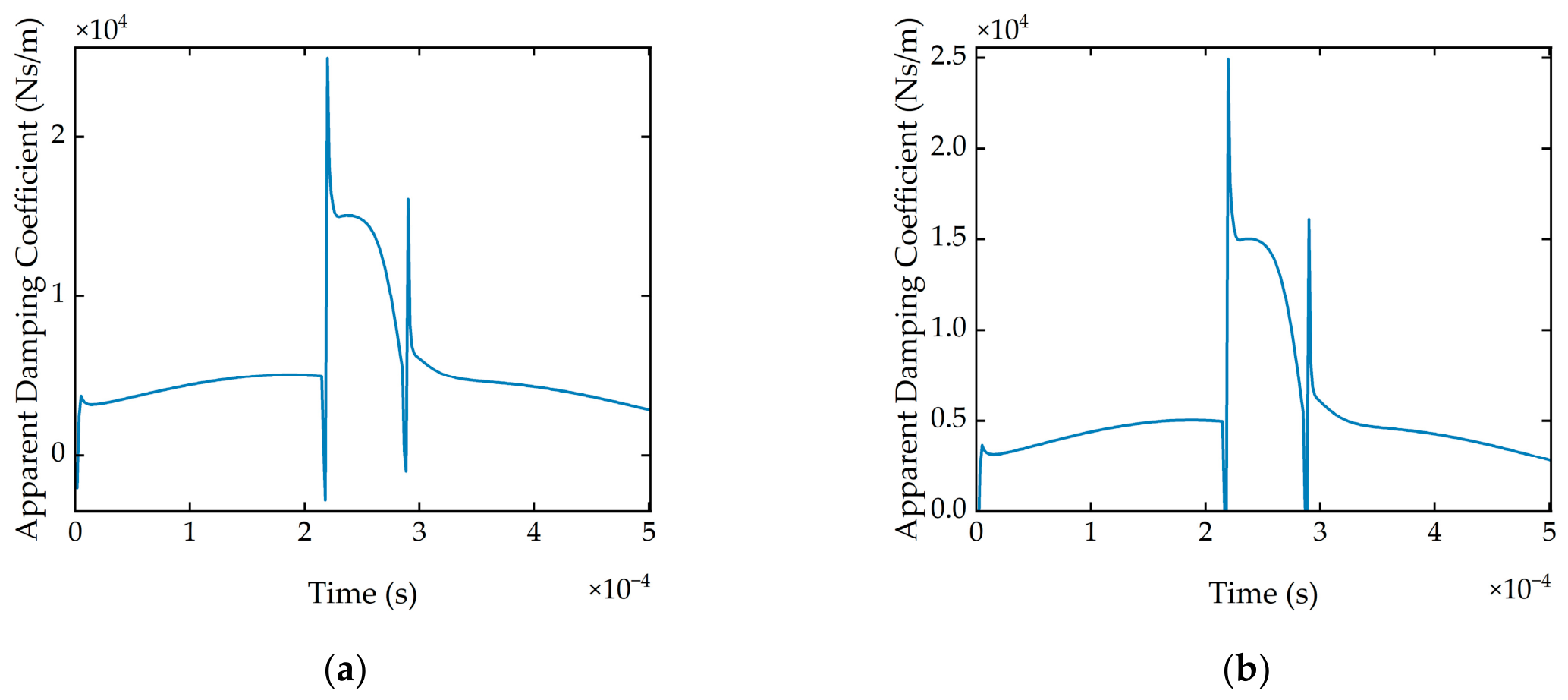
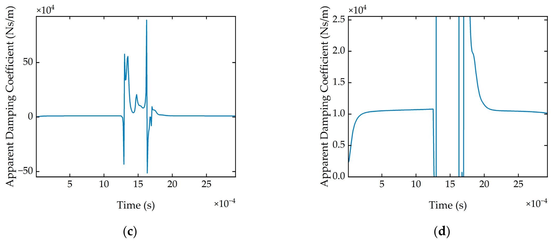
Figure A3.
Gear Pair 2 at (a) 100 Nm and 4200 RPM; (b) 100 Nm and 4200 RPM with zoomed y-axis; (c) 300 Nm and 720 RPM; (d) 300 Nm and 720 RPM with zoomed y-axis.
References
- Ishikawa, J. On the Deflection of Gear Teeth. Trans. Jpn. Soc. Mech. Eng. 1951, 17, 103–106. [Google Scholar] [CrossRef] [Scilit][Green Version]
- Japan Society of Mechanical Engineers. Gear Strength Design Data; The Japan Society of Mechanical Engineers: Tokyo, Japan, 1979; ISBN 978-4-88898-005-0. [Google Scholar]
- Weber, C. The Deformation of Loaded Gears and the Effect on Their Load-Carrying Capacity; Report; Sponsored Research (Germany), British Deptartment of Scientific and Industrial Research: London, UK, 1949; Volume 3. [Google Scholar]
- Weber, C.; Banaschek, K.; Niemann, G. Formänderung und Profilrücknahme bei gerad- und schrägverzahnten Rädern. In Schriftenreihe Antriebstechnik; Vieweg und Sohn: Braunschweig, Germany, 1955; Volume 11. [Google Scholar]
- Yang, D.C.H.; Lin, J.Y. Hertzian Damping, Tooth Friction and Bending Elasticity in Gear Impact Dynamics. J. Mech. Transm. Autom. Des. 1987, 109, 189–196. [Google Scholar] [CrossRef] [Scilit]
- Tian, X. Dynamic Simulation for System Response of Gearbox Including Localized Gear Faults. Master’s Thesis, University of Alberta, Edmonton, AB, Canada, 2004. [Google Scholar]
- Wu, S.; Zuo, M.J.; Parey, A. Simulation of Spur Gear Dynamics and Estimation of Fault Growth. J. Sound Vib. 2008, 317, 608–624. [Google Scholar] [CrossRef] [Scilit]
- Sainsot, P.; Velex, P.; Duverger, O. Contribution of Gear Body to Tooth Deflections—A New Bidimensional Analytical Formula. J. Mech. Des. 2004, 126, 748–752. [Google Scholar] [CrossRef] [Scilit]
- Mughal, H.; Sivayogan, G.; Dolatabadi, N.; Rahmani, R. An Efficient Analytical Approach to Assess Root Cause of Nonlinear Electric Vehicle Gear Whine. Nonlinear Dyn. 2022, 110, 3167–3186. [Google Scholar] [CrossRef] [Scilit]
- He, Z.; Wang, X.; Li, Y.; Yang, Y. Analysis of Gear System Dynamics Based on Thermal Elastohydrodynamic Lubrication Effects. Lubricants 2025, 13, 411. [Google Scholar] [CrossRef] [Scilit]
- Jian, G.; Wang, Y.; Zhang, P.; Xie, Y.; Zhao, J. Analysis of Lubricating Performance for Involute Spur Gear under Vibration. Lubr. Sci. 2020, 32, 344–357. [Google Scholar] [CrossRef] [Scilit]
- Zhou, C.; Xiao, Z.; Chen, S.; Han, X. Normal and Tangential Oil Film Stiffness of Modified Spur Gear with Non-Newtonian Elastohydrodynamic Lubrication. Tribol. Int. 2017, 109, 319–327. [Google Scholar] [CrossRef] [Scilit]
- Zhou, C.; Xiao, Z. Stiffness and Damping Models for the Oil Film in Line Contact Elastohydrodynamic Lubrication and Applications in the Gear Drive. Appl. Math. Model. 2018, 61, 634–649. [Google Scholar] [CrossRef] [Scilit]
- Xiao, Z.; Shi, X. Investigation on Stiffness and Damping of Transient Non-Newtonian Thermal Elastohydrodynamic Point Contact for Crowned Herringbone Gears. Tribol. Int. 2019, 137, 102–112. [Google Scholar] [CrossRef] [Scilit]
- Xiao, Z.; Zhou, C.; Chen, S.; Li, Z. Effects of Oil Film Stiffness and Damping on Spur Gear Dynamics. Nonlinear Dyn. 2019, 96, 145–159. [Google Scholar] [CrossRef] [Scilit]
- Li, Z.; Zhu, C.; Liu, H.; Gu, Z. Mesh Stiffness and Nonlinear Dynamic Response of a Spur Gear Pair Considering Tribo-Dynamic Effect. Mech. Mach. Theory 2020, 153, 103989. [Google Scholar] [CrossRef] [Scilit]
- Qin, W.; Chao, J.; Duan, L. Study on Stiffness of Elastohydrodynamic Line Contact. Mech. Mach. Theory 2015, 86, 36–47. [Google Scholar] [CrossRef] [Scilit]
- Yang, D.C.H.; Sun, Z.S. A Rotary Model for Spur Gear Dynamics. J. Mech. Transm. Autom. Des. 1985, 107, 529–535. [Google Scholar] [CrossRef] [Scilit]
- Wang, L.; Sun, L.; Zhao, N.; An, X.; Zhang, B.; Li, J. Time-Varying Mesh Stiffness Calculation by a Novel Loaded Tooth Contact Analysis Model Considering EHL Contact for Face-Gear Drive. Adv. Eng. Softw. 2025, 207, 103951. [Google Scholar] [CrossRef] [Scilit]
- Pei, J.; Han, X.; Tao, Y. An Improved Stiffness Model for Line Contact Elastohydrodynamic Lubrication and Its Application in Gear Pairs. Ind. Lubr. Tribol. 2020, 72, 703–708. [Google Scholar] [CrossRef] [Scilit]
- Fang, C.; Zhu, A.; Zhou, W.; Peng, Y.; Meng, X. On the Stiffness and Damping Characteristics of Line Contacts under Transient Elastohydrodynamic Lubrication. Lubricants 2022, 10, 73. [Google Scholar] [CrossRef] [Scilit]
- Tian, H.; Zhao, X.; Huang, W.; Ma, H. A Stiffness Model for EHL Contact on Smooth/Rough Surfaces and Its Application in Mesh Stiffness Calculation of the Planetary Gear Set. Tribol. Int. 2024, 196, 109720. [Google Scholar] [CrossRef] [Scilit]
- Lu, R.; Tang, W.; Xie, J.; Huang, Q.; Liu, X. A Unified Computational Framework for Meshing Stiffness of Spur Gears Incorporating Lubrication and Thermal Effects. Phys. Fluids 2025, 37, 063106. [Google Scholar] [CrossRef] [Scilit]
- Carrer, L.; Visnadi, L.B.; Tsuha, N.A.H.; Cavalca, K.L.; de Castro, H.F. A Novel Model of Lubricated Contact for Spur Gears. Mech. Mach. Theory 2026, 220, 106334. [Google Scholar] [CrossRef] [Scilit]
- Tsuha, N.A.H.; Nonato, F.; Cavalca, K.L. Formulation of a Reduced Order Model for the Stiffness on Elastohydrodynamic Line Contacts Applied to Cam-Follower Mechanism. Mech. Mach. Theory 2017, 113, 22–39. [Google Scholar] [CrossRef] [Scilit]
- Palmgren, A. Ball and Roller Bearing Engineering, 3rd ed.; S. H. Burbank and Company, Inc.: Philadelphia, PA, USA, 1959. [Google Scholar]
- Hoeprich, M.R.; Zantopulos, H. Line Contact Deformation: A Cylinder Between Two Flat Plates. J. Lubr. Technol. 1981, 103, 21–25. [Google Scholar] [CrossRef] [Scilit]
- Cooley, C.G.; Liu, C.; Dai, X.; Parker, R.G. Gear Tooth Mesh Stiffness: A Comparison of Calculation Approaches. Mech. Mach. Theory 2016, 105, 540–553. [Google Scholar] [CrossRef] [Scilit]
- Li, S.; Kahraman, A. A Transient Mixed Elastohydrodynamic Lubrication Model for Spur Gear Pairs. J. Tribol. 2010, 132, 011501. [Google Scholar] [CrossRef] [Scilit]
- Wiegert, B.; Hetzler, H.; Seemann, W. A Simplified Elastohydrodynamic Contact Model Capturing the Nonlinear Vibration Behaviour. Tribol. Int. 2013, 59, 79–89. [Google Scholar] [CrossRef] [Scilit]
- Townsend, D.P. Dudley’s Gear Handbook, 2nd ed.; McGraw-Hill: New York, NY, USA, 1992; ISBN 0070179034. [Google Scholar]
- Pedrero, J.I.; Pleguezuelos, M.; Artés, M.; Antona, J.A. Load Distribution Model along the Line of Contact for Involute External Gears. Mech. Mach. Theory 2010, 45, 780–794. [Google Scholar] [CrossRef] [Scilit]
- Messé, S.; Lubrecht, A.A. Transient Elastohydrodynamic Analysis of an Overhead Cam/Tappet Contact. Proc. Inst. Mech. Eng. Part J J. Eng. Tribol. 2000, 214, 415–425. [Google Scholar] [CrossRef] [Scilit]
- Szeri, A.Z. Fluid Film Lubrication: Theory and Design; Cambridge University Press: Cambridge, UK, 1998; ISBN 0-051-48100-7. [Google Scholar]
- Venner, C.H. Higher-Order Multilevel Solvers for the EHL Line and Point Contact Problem. J. Tribol. 1994, 116, 741–750. [Google Scholar] [CrossRef] [Scilit]
- Roelands, C.J.A. Correlational Aspects of the Viscosity-Temperature-Pressure Relationship of Lubricating Oils. Ph.D. Thesis, Technische Hogeschool, Delft, The Netherlands, 1966. [Google Scholar]
- Dowson, D.; Higginson, G.R. Elasto-Hydrodynamic Lubrication, 2nd ed.; Pergamon Press Ltd.: Oxford, UK, 1977; ISBN 0-08-021303-0. [Google Scholar]
- Venner, C.H. Multilevel Solution of the EHL Line and Point Contact Problems. Ph.D. Thesis, University of Twente, Enschede, The Netherlands, 1991. [Google Scholar]
- Venner, C.H.; Lubrecht, A.A. Multilevel Methods in Lubrication; Elsevier: Amsterdam, The Netherlands, 2000; ISBN 0444505032. [Google Scholar]
- Liu, S.; Wang, Q.; Liu, G. A Versatile Method of Discrete Convolution and FFT (DC-FFT) for Contact Analyses. Wear 2000, 243, 101–111. [Google Scholar] [CrossRef] [Scilit]
- Lubrecht, A.A. The Numerical Solution of the Elastohydrodynamically Lubricated Line- and Point Contact Problem Using Multigrid Techniques. Ph.D. Thesis, University of Twente, Enschede, The Netherlands, 1987. [Google Scholar]
- Shan, W.; Chen, Y.; Wang, X.; Yu, C.; Wu, K.; Han, Z. Nonlinear Dynamic Characteristics of Deep Groove Ball Bearings with an Improved Contact Model. Machines 2023, 11, 340. [Google Scholar] [CrossRef] [Scilit]
- Koshy, C.S.; Flores, P.; Lankarani, H.M. Study of the Effect of Contact Force Model on the Dynamic Response of Mechanical Systems with Dry Clearance Joints: Computational and Experimental Approaches. Nonlinear Dyn. 2013, 73, 325–338. [Google Scholar] [CrossRef] [Scilit]
- Chen, Y.; Lan, Q.; Wang, H.; Wu, X.; Zhang, X.; Wu, K. Nonlinear Analysis of Dynamic Behavior in a High-Precision Mechanism with a Revolute Clearance Joint. Lubricants 2026, 14, 122. [Google Scholar] [CrossRef] [Scilit]
- Tian, Q.; Flores, P.; Lankarani, H.M. A Comprehensive Survey of the Analytical, Numerical and Experimental Methodologies for Dynamics of Multibody Mechanical Systems with Clearance or Imperfect Joints. Mech. Mach. Theory 2018, 122, 1–57. [Google Scholar] [CrossRef] [Scilit]
- Chen, X.; Jiang, S. Nonlinear Dynamic Behavior Analysis of Multi-Linkage Mechanism with Multiple Lubrication Clearances. Eur. J. Mech.-B/Fluids 2022, 91, 177–193. [Google Scholar] [CrossRef] [Scilit]
- Blankenship, G.W.; Kahraman, A. Gear Dynamics Experiments: Part I—Characterization of Forced Response. In Proceedings of the 7th International Power Transmission and Gearing Conference; ASME: San Diego, CA, USA, 1996; pp. 373–380. [Google Scholar]
- Guilbault, R.; Lalonde, S.; Thomas, M. Nonlinear Damping Calculation in Cylindrical Gear Dynamic Modeling. J. Sound Vib. 2012, 331, 2110–2128. [Google Scholar] [CrossRef] [Scilit]
- Mughal, H.; Dolatabadi, N.; Rahmani, R. An Integrated Tribodynamic Model for Investigation of Efficiency, Durability and NVH Attributes of Gear Mesh in Electric Vehicle Powertrains. Tribol. Int. 2023, 189, 108977. [Google Scholar] [CrossRef] [Scilit]
- Cornell, R.W. Compliance and Stress Sensitivity of Spur Gear Teeth. J. Mech. Des. 1981, 103, 447–459. [Google Scholar] [CrossRef] [Scilit]
- Johnson, K.L. Contact Mechanics; Cambridge University Press: Cambridge, UK, 1985; ISBN 0521347963. [Google Scholar]

Disclaimer/Publisher’s Note: The statements, opinions and data contained in all publications are solely those of the individual author(s) and contributor(s) and not of MDPI and/or the editor(s). MDPI and/or the editor(s) disclaim responsibility for any injury to people or property resulting from any ideas, methods, instructions or products referred to in the content. |
© 2026 by the authors. Licensee MDPI, Basel, Switzerland. This article is an open access article distributed under the terms and conditions of the Creative Commons Attribution (CC BY) license.