


Abstract
To address the limitations of conventional magnetorheological (MR) fluid hydrostatic bearings, a variable-stiffness bearing is proposed. These limitations include insufficient load capacity, low torque margin, and poor adaptability under complex operating conditions. Taking MR fluid as the lubricating medium, the device adopts permanent magnets to provide a basic stable magnetic field. A dual-excitation configuration, consisting of stiffness-adjustment coils integrated into the bearing and shaft-mounted coils attached to the rotor, enables dynamic magnetic field regulation. This mechanism modulates the rheological behavior of the MR fluid, realizing flexible stiffness tuning and dynamic torque enhancement of the bearing. The overall structure and working principle of the device are elaborated in detail. The mathematical models of bearing stiffness-current and output torque-current are derived, and the regulation law of current on the dynamic characteristics of the bearing is clarified. Ansys Maxwell 2022 R1 simulation results verify the feasibility of the dual excitation decoupling control scheme. The research results can provide theoretical support and technical reference for the intelligent regulation and engineering application of MR fluid hydrostatic bearings.
1. Introduction
Hydrostatic bearings have low friction and high rotational accuracy. They also provide strong vibration resistance and load support. Therefore, they are widely used in high-end equipment. Typical applications include CNC machine tool spindles, mining transmission systems, wind turbine shafts, and aero-engines. They are key basic components in the field of heavy and precision equipment [1,2,3]. With the development of high-end equipment towards high speed, heavy load, and intelligence, the operating conditions of the equipment have become increasingly complex. Scenarios such as strong load disturbance, wide speed range fluctuation, and extreme condition impact have put forward higher requirements for the stiffness tunability, load torque margin, and working condition adaptive capability of hydrostatic bearings [4,5].
Traditional liquid-lubricated hydrostatic bearings use lubricating oil with fixed viscosity as the lubricating medium. To further illustrate the limitations of the lubrication performance of traditional fixed viscosity hydrostatic bearings, the Stribeck curve theory is introduced here. The Stribeck curve describes the variation in bearing friction coefficient and divides bearing lubrication into three states: boundary lubrication, mixed lubrication, and full fluid film lubrication. Traditional oil-lubricated bearings are prone to getting stuck in boundary/mixed lubrication at low speeds and heavy loads, accompanied by severe friction and wear. Under high-speed operating conditions, the temperature of the lubricating oil increases. This leads to a significant reduction in viscosity, resulting in decreased load-carrying capacity and stiffness of the bearing. Under sudden loading and strong disturbance conditions, bearings with fixed stiffness cannot adapt quickly to load variations. This may lead to shaft runout and lubrication failure, which negatively affect operating accuracy and system safety [6,7,8]. Therefore, the development of intelligent hydrostatic bearings with dynamic stiffness tunability and active load torque enhancement capability has become an urgent key problem to be solved in the field of bearing technology.
MR fluid is an intelligent material composed of magnetic particles, carrier liquid, and additives. Under an external magnetic field, it transforms from a Newtonian fluid to a Bingham plastic within milliseconds. Its yield stress increases with magnetic field strength in a reversible manner. This property is known as the magnetorheological effect [9,10,11]. Where Newtonian fluid exhibits a linear relationship between shear stress and shear rate, and constant viscosity is independent of the external field. In contrast, MR fluids behave as Bingham plastics under applied magnetic fields, characterized by field-dependent yield stresses. The shear yield stress must be exceeded before MR begins to flow under a magnetic field. Compared with conventional lubricating oil, MR hydrostatic bearings maintain a complete oil film through external oil supply. At the same time, its viscosity can be continuously adjusted by a magnetic field, actively changing the Hessian number, expanding the effective working range of full fluid lubrication, and avoiding high friction zones under complex working conditions. Therefore, MR fluid is suitable for intelligent lubrication and active performance control of bearings [12,13].
In recent years, scholars have investigated MR fluid bearings. Research progress has been made in structural design, magnetic field optimization, and performance modeling [14,15,16]. In terms of the structural design of MR fluid hydrostatic bearings, relevant studies have proposed an active MR fluid hydrostatic bearing structure. Through hybrid excitation by permanent magnets and energized coils, the magnetorheological effect is used to increase the flow damping of the lubricating medium, which effectively improves the static load-bearing capacity of the bearing [17,18]. Some scholars have conducted simulation-based optimization of the magnetic field distribution in MR bearings. These studies clarify the influence of excitation structure parameters on the magnetic flux density in the lubrication gap. The results provide a theoretical basis for structural optimization of MR bearings [19,20,21]. In terms of bearing performance control, existing studies have introduced displacement feedback and semi-active control strategies. By dynamically adjusting the input current of the excitation coil, the closed-loop adjustment of bearing lubrication parameters and support characteristics is realized, and the anti-disturbance capability of the bearing is improved [22,23,24]. At the same time, scholars have established a stiffness calculation model for MR fluid lubricated bearings, and verified the feasibility of adjusting bearing stiffness through magnetic field control [25,26,27].
However, based on the comprehensive analysis of existing studies, the current technologies related to MR fluid hydrostatic bearings still have obvious limitations. Meer et al. [28] proposed that under higher loads, the relative improvement in load-carrying performance provided by MR lubrication decreases significantly, indicating limited effectiveness under high-load conditions. Lampaert et al. [29] reported that the load-carrying capacity of hydrostatic bearings lubricated with MR fluids increases with magnetic field intensity; however, the improvement is strongly dependent on operating conditions and does not scale proportionally with magnetic excitation. Wodtke et al. [8] proposed that MR-lubricated bearings exhibit approximately six times higher friction coefficient compared to oil lubrication, indicating significantly reduced torque margin under practical operating conditions.
To address the above problems, this paper designs a variable stiffness MR fluid hydrostatic bearing device with a dual excitation structure. This device utilizes permanent magnets to provide a basically stable magnetic field, and achieves decoupling control of stiffness and torque through two independent sets of coils. This paper elaborates the overall structure and working principle of the device in detail. Based on the Bingham constitutive model of MR fluid and the lubrication theory of hydrostatic bearings, the mechanistic mathematical models of bearing stiffness-current and output torque-current are derived. The simulation analysis of the internal magnetic field distribution characteristics of the bearing is carried out through the Ansys Maxwell 2022 R1 finite element software. The research in this paper can provide a new structural scheme and theoretical support for the intelligent active control of MR fluid hydrostatic bearings.
2. Design of MR Bearing with Variable Stiffness
2.1. Overall Structure
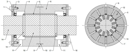
The variable stiffness MR fluid hydrostatic bearing device proposed in this paper utilizes MR fluid as the lubricating medium and achieves active adjustment of support stiffness and load torque through magnetic field regulation. The bearing device primarily consists of six components: the bearing body, stepped shaft, permanent magnet, dual excitation coil system, oil circuit system, and axial fixing and sealing structure. The overall structure is illustrated in Figure 1.
Figure 1.
Structure of MR bearing with variable stiffness. 1—shaft end retaining ring, 2—skeleton seal, 3—screw, 4—lock nut, 5—permanent magnet, 6—bushing, 7—rotating shaft, 8—first oil outlet, 9—oil inlet, 10—oil cavity, 11—second oil outlet, 12—stiffness adjustment coil, 13—shaft-mounted coil, 14—first axis segment, 15—second axis segment, 16—third axis segment, 17—fourth axis segment, 18—fifth axis segment.
The rotating shaft (7) adopts a five-segment symmetrical stepped structure, including a first axis segment (14), a second axis segment (15), a third axis segment (16), a fourth axis segment (17), and a fifth axis segment (18). The third axis segment (16) is the central working axis segment, and the remaining segments are distributed symmetrically. The second and fourth segments are threaded for axial positioning and fastening. There are multiple sets of permanent magnets (5) uniformly embedded on the inside of the bushing (6), with axial fixation achieved by lock nuts (4) on both sides. The stiffness adjustment coil (12) is wound around the winding frame where the permanent magnets (5) are located. Multiple sets of shaft-mounted coils (13) are uniformly attached to the outside of the third segment of the rotating shaft (7), forming a dual excitation coil system.
2.2. Compound Excitation System
The compound excitation system consists of three parts: permanent magnets (5), stiffness adjustment coils (12), and shaft-mounted coils (13), and is the core for achieving dynamic regulation and control of bearing performance. The permanent magnets (5) are magnetized radially to provide a continuous and stable basic magnetic field for the bearing lubrication gap, ensuring that the bearing has stable basic stiffness and load-bearing capacity when there is no current input. The stiffness adjustment coils (12) are wound around the permanent magnets (5) inside the bushing (6). When energized, they magnetize the first oil seal edge, and the generated magnetic field superimposes in the same direction as the basic magnetic field of the permanent magnets (5), allowing for continuous adjustment of the magnetic field strength within the lubrication gap. The shaft-mounted coils (13) are fixed to the central shaft section of the stepped rotating shaft (7). When energized, it magnetizes the second oil seal edge, and the generated magnetic field forms a magnetic repulsion force with the basic magnetic field of the permanent magnets (5), providing auxiliary driving torque for the rotation of the rotating shaft (7) and enhancing the load-bearing torque of the bearing.
2.3. Oil Circuit and Sealing Structure
The oil circuit system adopts the symmetric structure of “four inlets and two outlets”, and four radial oil holes (9) ensure sufficient oil supply capacity under high load or disturbance conditions to avoid pressure collapse caused by insufficient oil supply on one side. Symmetric arrangement can reduce the initial pressure deviation caused by the difference in oil supply path and improve the static stability of the system. The first oil outlet (8) and the second oil outlet (11) are symmetrically arranged under the bearing to ensure smooth oil return of the lubrication circuit and maintain stable pressure of the oil cavity (10).
When eccentricity occurs, the bearing side oil film thickness decreases, the fluid resistance increases, and the corresponding oil chamber pressure automatically rises, forming the restoring force against the eccentricity. At this time, the stiffness-regulating coil is energized. Under the applied magnetic field, the MR fluid exhibits the magnetorheological effect, and its apparent viscosity increases. This enhances the difference in hydraulic resistance between oil chambers, further amplifying the pressure variation and improving the restoring capability of the bearing. Therefore, the bearing capacity of the bearing is increased and the slewing accuracy is improved.
The sealing structure adopts a double-sided skeleton seal (2), which is installed on the left and right ends of the bushing (6) respectively, and is interference-fitted with the shaft section of the rotating shaft (7). It can effectively block the leakage of MR fluid along the axial gap, ensure the filling rate of MR fluid in the lubrication gap and the stability of the oil chamber pressure, and prevent external dust and impurities from entering the bearing interior.
3. Stiffness and Torque Adjustment of MR Fluid
This device utilizes MR fluid as the lubricating medium. The MR fluid enters the bearing oil chamber through the oil inlet hole, fills the lubrication gap between the shaft sleeve and the rotating shaft, and then flows out through the radial oil outlet hole. A circulating lubrication loop is thereby formed. The core working principle of the device is divided into two dimensions: stiffness adjustment and torque enhancement.
The mathematical models for bearing stiffness and output torque are developed in this study. They are based on Reynolds lubrication theory for hydrostatic bearings, the Bingham plastic constitutive model for MR fluid, and laminar flow resistance theory in parallel gaps. The following general basic assumptions are adopted to simplify the complex multi-field coupling relationship and ensure the engineering applicability of the model:
- The MR lubricating fluid is incompressible, and the flow inside the lubrication gap is steady laminar flow;
- Fluid inertia force and viscosity variation caused by temperature rise are neglected, and isothermal modeling is adopted;
- The bearing operates under a small eccentricity condition e/h0 ≤ 0.3, with a limited range variation of oil film thickness;
- The oil supply pressure is stable, the oil supply flow of four oil cavities is consistent, and no external flow disturbance exists;
- The magnetic circuit is weakly coupled with the fluid lubrication field, and the correlation is only established by adjusting the equivalent viscosity of MR fluid via the magnetic field.
3.1. Principle of Stiffness Adjustment
Permanent magnets provide a basic magnetic field for the lubrication gap, giving MR fluid basic shear yield stress and viscosity that correspond to the basic stiffness of the bearing. When an adjustable current is applied to the stiffness adjustment coil, an additional magnetic field is generated. This magnetic field is superimposed on the permanent magnet field at the oil sealing edge in the same direction. The magnetic field strength within the lubrication gap increases with the increase in input current, leading to an increase in the shear yield stress and viscosity of the MR fluid. As a result, the flow resistance across the oil sealing edge is significantly increased, leading to higher oil chamber pressure and improved bearing load capacity and support stiffness. On the contrary, inputting a reverse current can reduce the bearing stiffness. By continuously adjusting the current of the stiffness adjustment coil, wide-range, fast, and reversible adjustment of bearing stiffness can be realized.
Oil film stiffness represents the ratio of load change to radial displacement change, and is the ability of the bearing to resist deformation
where is the oil film stiffness of the bearing, N/m; is the load-bearing capacity of the bearing, N; and is the radial eccentricity (variation in oil film thickness), m.
The load-bearing capacity of a four-oil-cavity symmetric hydrostatic bearing is determined by the effective load-bearing area and the pressure difference across the oil cavities
where is the effective bearing area of the oil cavity, m2, and is the pressure difference between the opposing oil cavities, Pa.
The pressure difference is proportional to the lubrication gap fluid resistance, which is related to the viscosity of the MR fluid and the oil film gap
where is a structural constant; is the viscosity of the MR fluid controlled by magnetic field B (scale factor between shear stress and shear rate), Pa·s; and is the radial clearance of the bearing, m.
The stiffness of the bearing consists of two parts: the basic stiffness provided by the permanent magnet and the controllable stiffness provided by the stiffness adjustment coil
where is the basic stiffness provided by the permanent magnet, N/m; is the variable stiffness provided by the stiffness adjustment coil, N/m; is the stiffness adjustment coefficient; is the basic magnetic field of the permanent magnet, T; is the current-to-magnetic field conversion coefficient; and is the current of the stiffness adjustment coil, A.
It should be noted that the stiffness-current relationship presented in this study is a locally linearized approximation based on the nominal operating point.
In reality, the viscosity of MR fluid exhibits a nonlinear dependence on magnetic field intensity, typically described by a Herschel–Bulkley-type constitutive model, while the bearing stiffness is also strongly influenced by the cubic relationship with film thickness (h3).
Therefore, Equations (4) and (5) are established under the assumption of small perturbations around steady operating conditions, where the magnetic field remains in the unsaturated region and the variation in film thickness is limited. Within this range (0–3 A excitation current), the linear approximation provides acceptable accuracy for control-oriented analysis.
3.2. Principle of Torque Improvement
When an adjustable current is applied to the shaft-mounted coil, a magnetic field is generated. This field interacts with the magnetic field of the permanent magnet near the second oil seal edge. The interaction results in a repulsive magnetic effect due to opposite field directions. This magnetic repulsion force is converted into an auxiliary driving torque for the shaft rotation, effectively counteracting the frictional resistance torque during the bearing’s operation, thereby enhancing the output load torque of the bearing. By adjusting the magnitude of the current flowing through the shaft-mounted coil, the auxiliary driving torque can be linearly regulated, achieving flexible control of the bearing’s load torque.
The total load torque consists of three parts
where is the total load torque of the bearing, N·m; is the base oil film friction torque, N·m; is the additional oil film torque induced by the stiffness adjustment coil, N·m; and is the auxiliary magnetic repulsion torque generated by the shaft-mounted coil, N·m.
where is the shaft radius, m; is the bearing length, m; is the oil film shear stress, Pa; is the zero-flow shear yield stress of the MR fluid under the permanent magnet base magnetic field, Pa; η0 is the base viscosity, Pa·s; v is the tangential velocity of the shaft surface, m/s; and is the oil film gap, m.
where is MR shear stress under stiffness adjustment coil current, Pa; is the current of the stiffness adjustment coil, A; is the basic magnetic field of the permanent magnet, T; are the nonlinear coefficients of the MR fluid; and is the viscosity of the MR fluid under the magnetic field, which increases with the increase in current, Pa·s.
where is the current of the shaft-mounted coil, A; is the effective magnetic area of the coil, m2; and is the magnetic repulsion conversion coefficient, which converts magnetic force into torque.
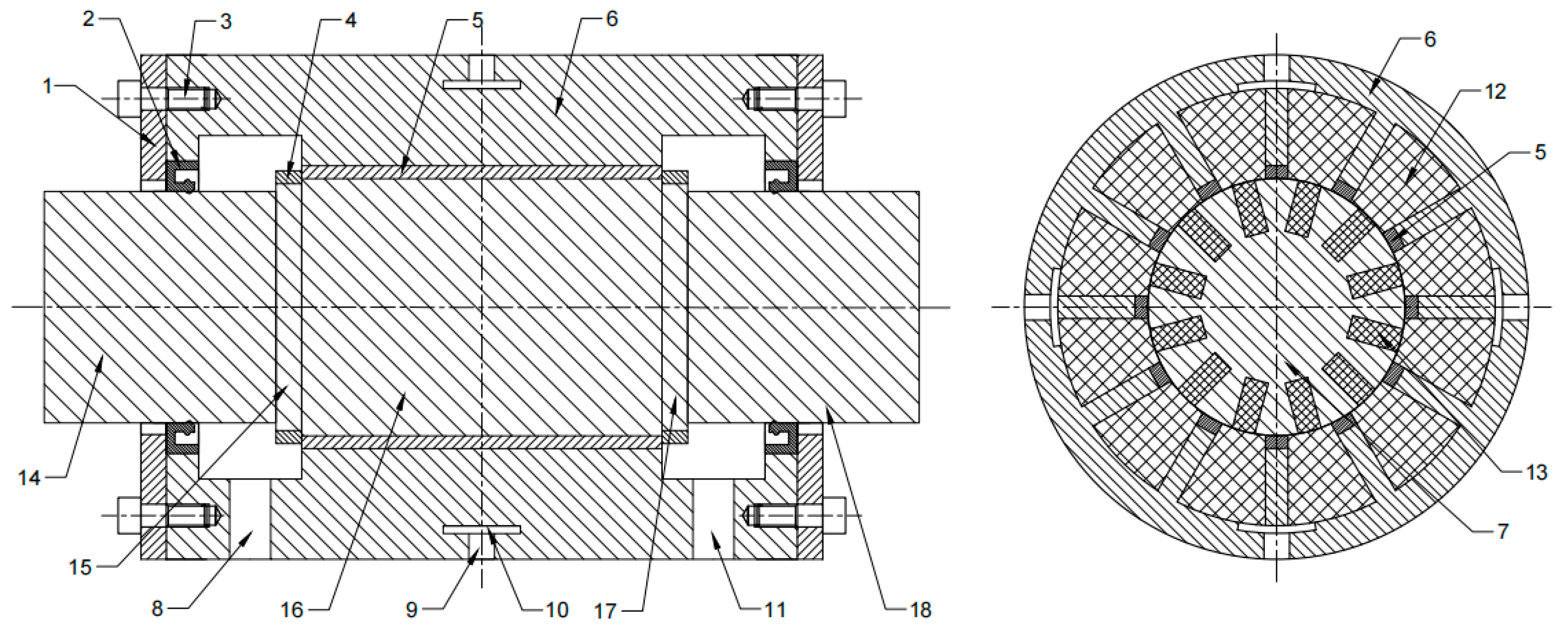
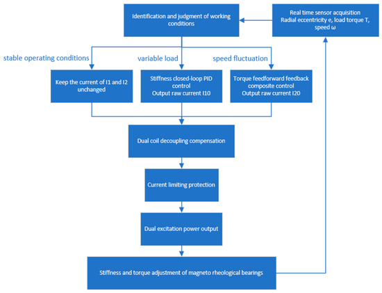
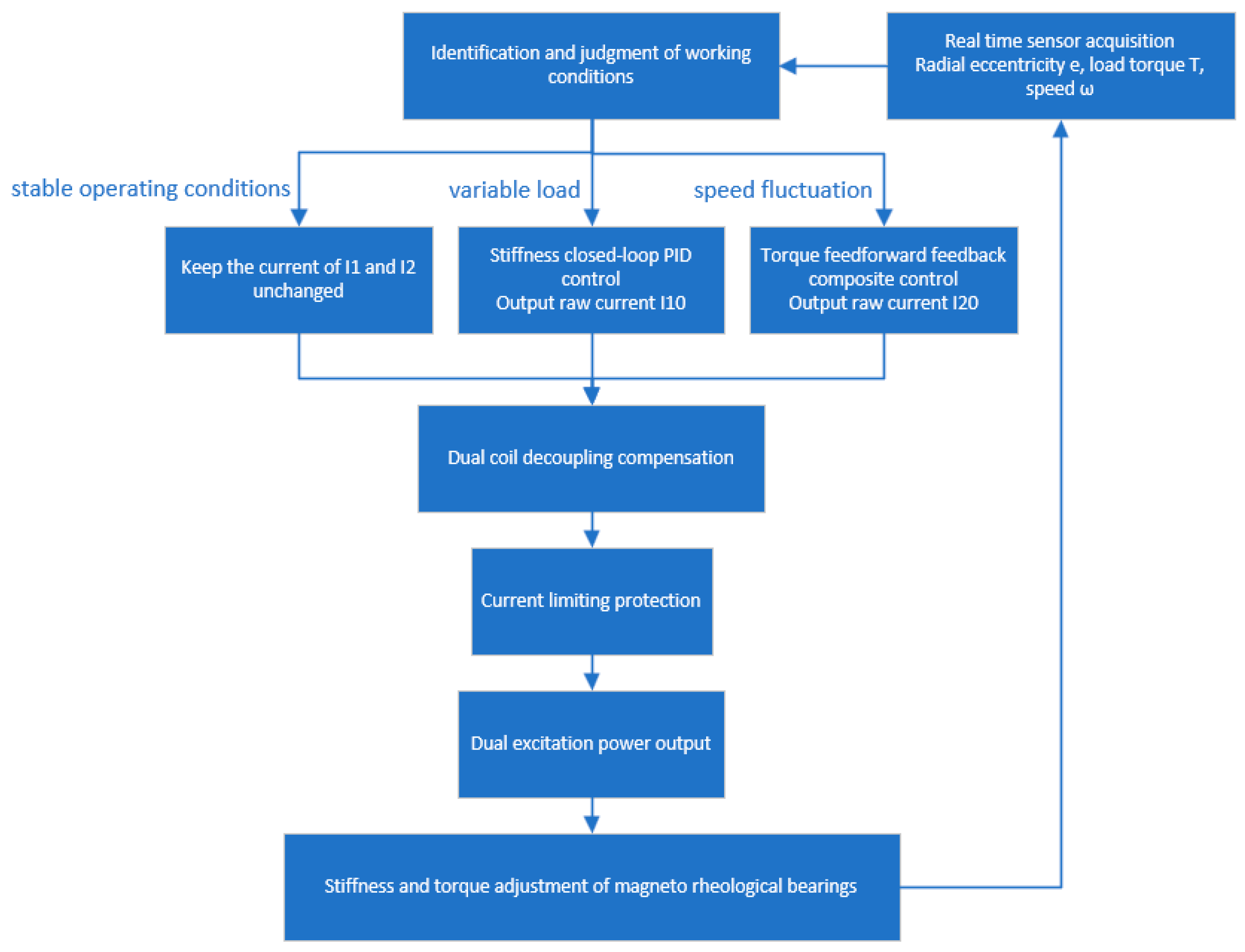
Based on the aforementioned working principle, this device can achieve dynamic adjustment of bearing stiffness and active enhancement of load-bearing torque through independent or coordinated control of two sets of coils. This enables the bearing to quickly adapt to complex working conditions such as heavy loads, variable loads, and strong disturbances, significantly improving operational stability. The relevant algorithm flowchart is shown in Figure 2.
Figure 2.
Control algorithm flowchart.
Taking rotor radial eccentricity, load torque and shaft speed as feedback inputs, the system distinguishes three operating states (steady state, variable load and speed fluctuation) through the operating condition judgment unit. For non-steady working conditions, displacement PID closed-loop stiffness control and speed feedforward-feedback composite torque control are adopted to calculate two groups of original excitation currents, respectively. Magnetic field decoupling compensation is implemented to eliminate cross-coupling interference between coils, and current amplitude limiting is applied to avoid magnetic saturation and coil overheating. Finally, two channels of driving currents are output to cooperatively adjust the stiffness and output torque of the magnetorheological bearing, forming a complete closed-loop adaptive regulation system.
4. Magnetic Circuit Design in MR Fluid Bearing
4.1. Calculation of Magnetic Resistance
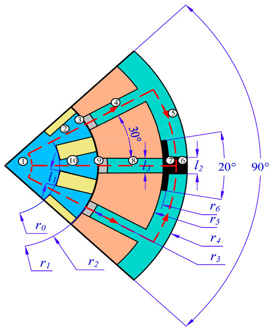
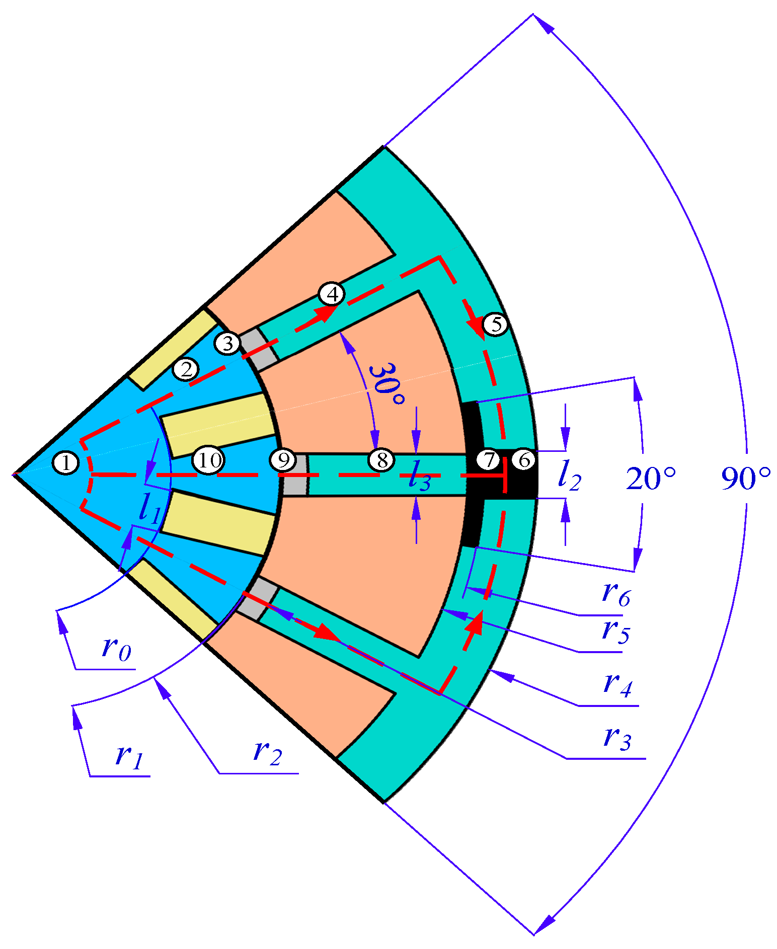
The magnetic circuit of the MR fluid bearing is simplified, and a simplified magnetic circuit is obtained based on different material distributions and cross-sectional areas, as shown in Figure 3. The meaning of each label in the figure is as follows: 1 represents the circumferential magnetic circuit of the rotor part, 2 and 10 represent the radial magnetic circuit of the rotor between the shaft-mounted coils, 4 and 8 represent the radial magnetic circuit of the stator part, 5 represents the circumferential magnetic circuit of the stator part, 6 and 7 represent the magnetic circuit of the MR fluid inlet part, and 3 and 9 represent the magnetic circuit of the MR fluid gap.
Figure 3.
Schematic diagram of the magnetic circuit composition.
The magnetic reluctance of each segment in the magnetic circuit can be calculated according to magnetic Ohm’s law. The calculation method for circumferential magnetic reluctance is as follows:
The calculation of radial partial magnetic resistance can be expressed as follows:
where is the magnetic reluctance of each part of the magnetic circuit, H−1; is the circumferential angle of each part of the magnetic circuit; is the length of each part of the magnetic circuit, m; is the outer diameter of each part of the circumference, m; is the inner diameter of each part of the circumference, m; is the magnetic permeability of the material, H/m; is the cross-sectional area of each part of the magnetic circuit, m2; and is the code of the magnetic circuit.
By calculating the magnetic resistance of each segment in turn, we can obtain
The specific dimensions and material parameters of the MR fluid bearing are shown in Table 1.
Table 1.
The main geometric and material parameters of the magnetic circuit.
In this study, an equivalent linear permeability model was used to reduce the complexity of the model and obtain an analytical solution. This value is the average equivalent relative permeability of the oil-based MR fluid in the operating magnetic field range of 0.1~0.6 T, which can meet the accuracy requirements of the preliminary magnetic circuit design.
4.2. Permanent Magnet Calculation
According to the different positions and relationships of magnetic resistance in the magnetic circuit, we can note that
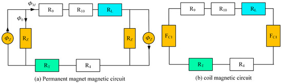
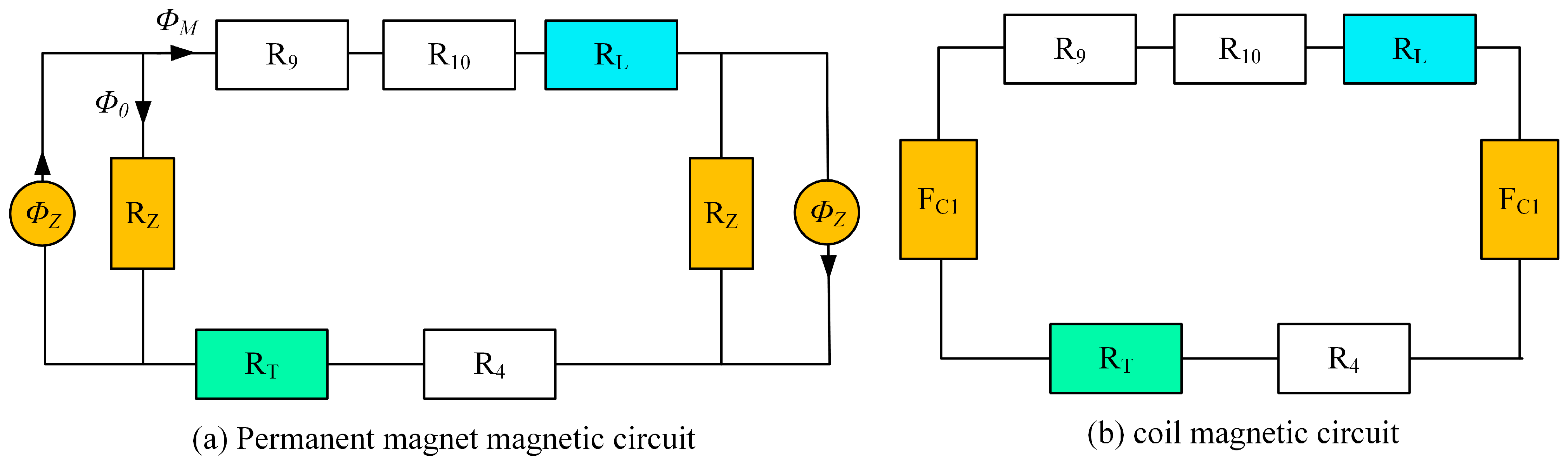
When considering the effect of permanent magnets on the magnetic circuit alone, the equivalent magnetic circuit is shown in Figure 4a; when considering the effect of coils on the magnetic circuit alone, taking into account that the magnetic reluctance of the permanent magnet branch is much greater than that of the MR fluid working gap branch, the corresponding equivalent magnetic circuit model is shown in Figure 4b.
Figure 4.
Equivalent magnetic circuit.
The permanent magnet is equivalent to a constant magnetic flux source model with internal magnetic reluctance connected in parallel. The relationship between the effective magnetic flux and the internal magnetomotive force of the permanent magnet can be derived from the fundamental laws of magnetic circuits
where represents the effective magnetic flux provided by the permanent magnet to the external magnetic circuit, ; represents the virtual leakage magnetic flux inside the permanent magnet, ; and represents the internal magnetic reluctance of the permanent magnet, .
To achieve a wider stiffness adjustment range, ferrite of grade Y22H is selected as the permanent magnet material. The calculation of its magnetomotive force is as follows:
where is the coercivity of the permanent magnet material, , and is the effective length of the permanent magnet along the magnetization direction, m.
4.3. Coil Calculation
To calculate the required excitation ampere-turns for the coil, it is necessary to first determine the magnetic flux variation in the working gap of the MR fluid under the separate actions of the permanent magnet and the coil. When the permanent magnet acts alone, the magnetic induction intensity in the MR fluid gap is , corresponding to a magnetic circuit flux of . Under the excitation of the stiffness adjustment coil, the magnetic induction intensity in the working gap needs to be increased to a maximum value of , corresponding to a magnetic circuit flux of .
The total magnetic reluctance of the coil magnetic circuit is
According to Ohm’s Law in magnetic circuits, the magnetomotive force (MMF) required to be provided by a coil branch is equal to the product of the increment of magnetic flux and the total magnetic reluctance of the loop. Assuming the number of coil turns is N and the excitation current is I, the required ampere-turns of the coil can be obtained from Kirchhoff’s Second Law as follows:
Using the aforementioned formula, the required magnetomotive force to enhance the magnetic induction intensity of the MR fluid gap to 0.5 T through the stiffness adjustment coil can be calculated as follows: , and the magnetomotive force required to counteract the magnetic force of the permanent magnet is: . Taking all factors into consideration, a copper wire with a diameter of 1mm is selected for winding the coil, with a total of 800 turns.
5. Magnetic Field Simulation Analysis of MR Bearing
5.1. Pre-Processing Simulation
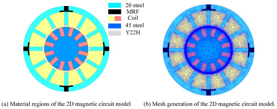
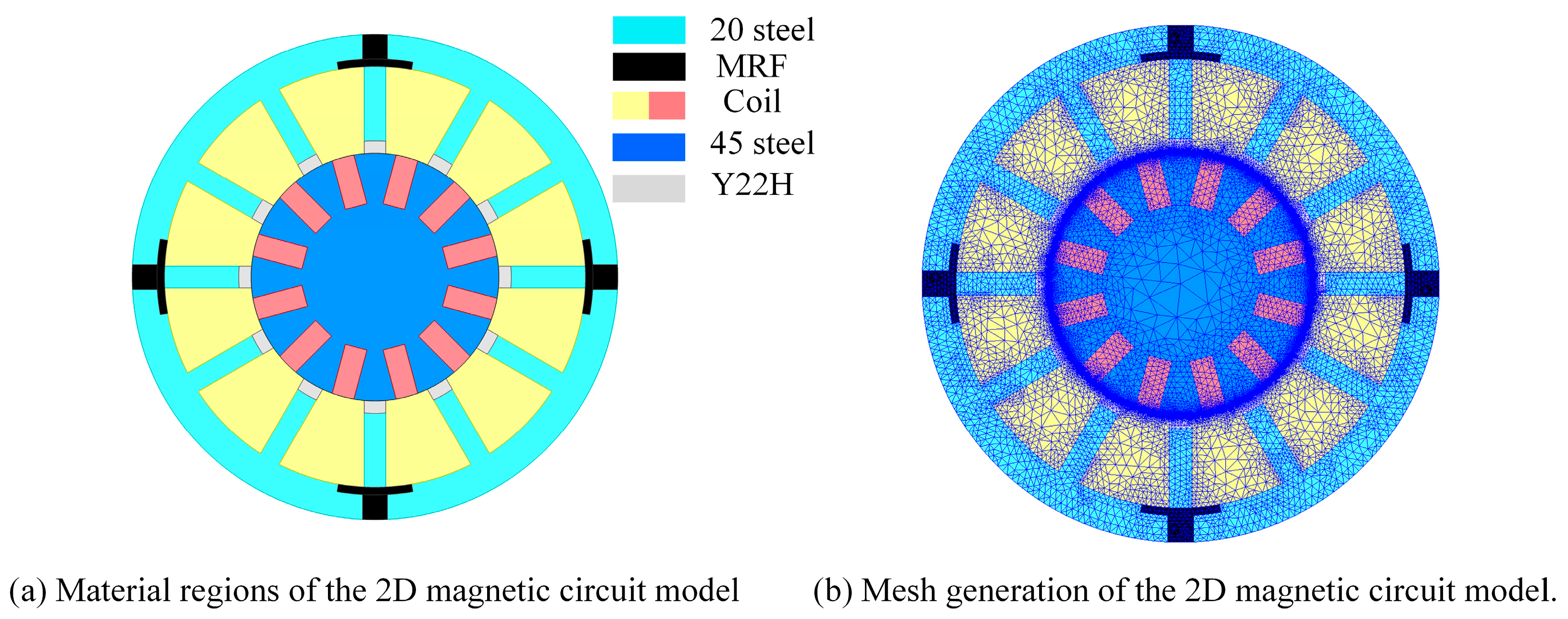
To verify the rationality of the magnetic circuit design and the accuracy of the theoretical model, numerical simulation of the MR fluid bearing was carried out using the electromagnetic field finite element method. Due to the original geometric model containing a large number of detailed structures, directly performing full-scale modeling would significantly increase the grid scale, reduce the efficiency of the solution, and even affect the convergence of the calculation. Therefore, it is necessary to appropriately simplify the model while ensuring that the key electromagnetic characteristics are not distorted.
During the construction of the two-dimensional electromagnetic field model, local structural features that have a minor impact on the overall magnetic field distribution, such as side magnetic holes, bolt holes, and non-load-bearing auxiliary structures, are neglected. Meanwhile, adjacent components with consistent material properties and identical functions in the magnetic circuit are equivalently merged to reduce unnecessary contact interfaces and complex boundary conditions, thereby reducing model complexity and enhancing computational efficiency.
In terms of grid division, for key areas with large magnetic flux density gradients, a local densification strategy is adopted to improve the resolution and accuracy of magnetic field distribution calculations. In areas where the magnetic field changes relatively smoothly, a coarser grid division is used to achieve a reasonable balance between calculation accuracy and solution efficiency. The material distribution and grid division of each component in the finite element model established based on the above modeling principles are shown in Figure 5.
Figure 5.
The simplified magnetic circuit model.
5.2. Influence of Stiffness Adjustment Coil Current on Magnetic Field Distribution
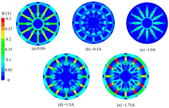
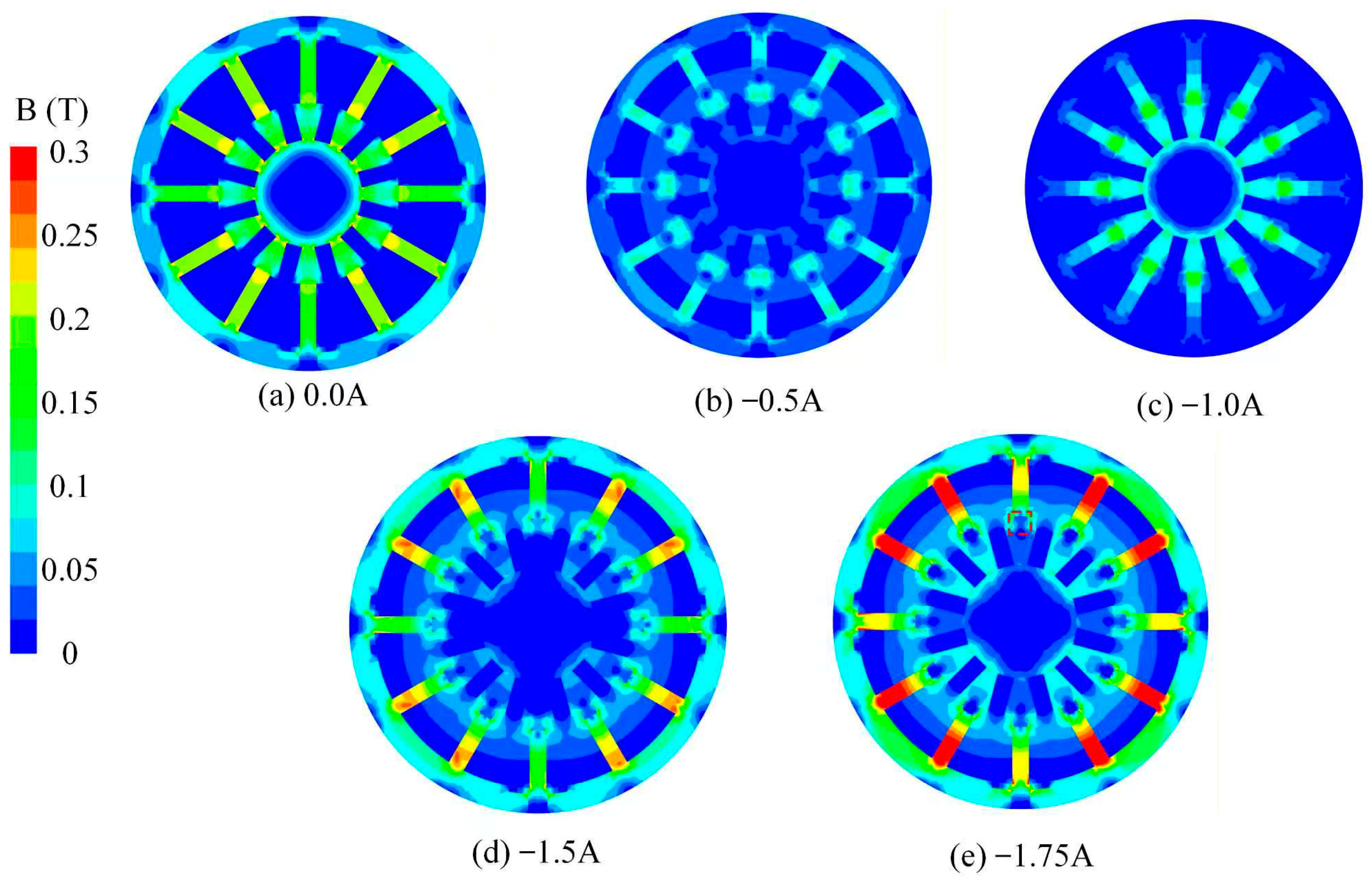
Figure 6 presents the contour plots of magnetic induction intensity distribution for the stiffness adjustment coil under different reverse currents. Under the condition of no power or only a small current being applied, the magnetic field is primarily provided by the permanent magnet, and the magnetic flux closes along a path with less magnetic resistance. The distribution of magnetic induction intensity within the working gap is relatively stable, but the overall adjustment range is limited. As the reverse current gradually increases, the direction of the magnetomotive force generated by the stiffness adjustment coil is opposite to that of the permanent magnet’s magnetic field, gradually canceling out the original magnetic flux. This results in an overall downward trend in the magnetic induction intensity within the working gap, while the magnetic flux density in some local areas of the stator first decreases and then increases.
Figure 6.
Distribution gradient of magnetic flux density under different reverse currents.
From the perspective of the magnetic circuit mechanism, the introduction of reverse excitation weakens the dominant role of the permanent magnets in the main magnetic circuit. It changes the magnetic flux distribution among different branches. As a result, the magnetic field in the working gap becomes more adjustable, and its regulation range is expanded. Due to the high sensitivity of the yield stress and equivalent stiffness of MR fluids to magnetic induction intensity, a decrease in the gap magnetic field will directly lead to a weakening of its mechanical properties. Therefore, by applying a reverse current, active regulation of the magnetic induction intensity in the working gap can be achieved, thereby achieving the goal of reducing equivalent stiffness and realizing stiffness softening adjustment.
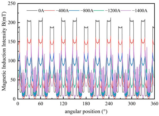
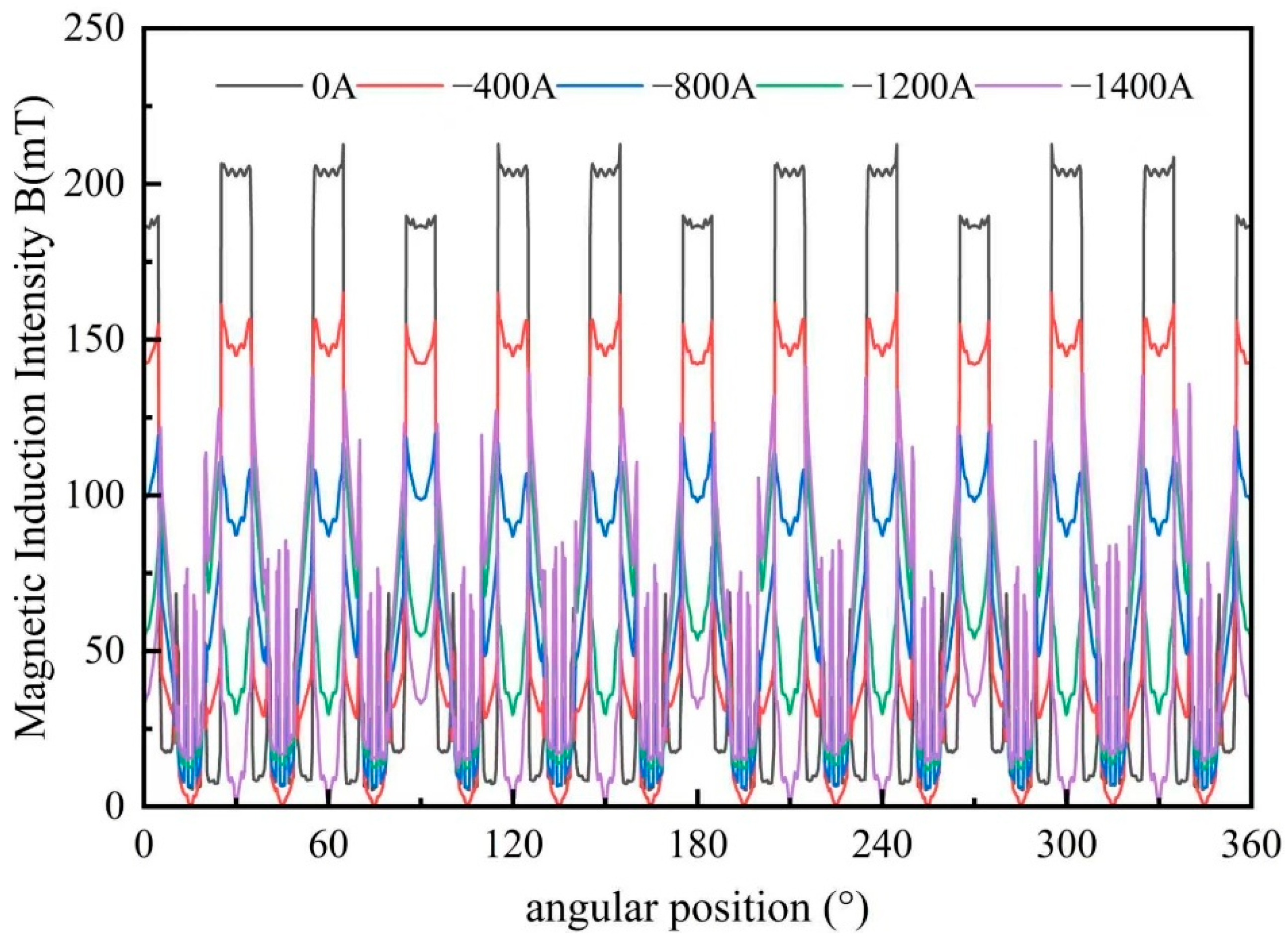
Figure 7 depicts the variation curve of magnetic induction intensity along a specific path in the working gap under different reverse currents. The results indicate that the distribution of magnetic induction intensity along the path is not entirely flat, but exhibits local elevation in the magnetic flux convergence region and a certain gradient change in the geometric transition zone. As the reverse current increases, the curve shifts downward overall, indicating that the coil’s counteraction to the permanent magnetic field intensifies. Simultaneously, the magnitude of change in magnetic induction intensity in the central region of the gap is smaller than that in the edge region, suggesting that this area possesses superior magnetic field stability and higher magnetic flux utilization efficiency.
Figure 7.
Relationship curve of magnetic flux density with angular position under different reverse currents.
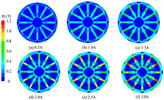
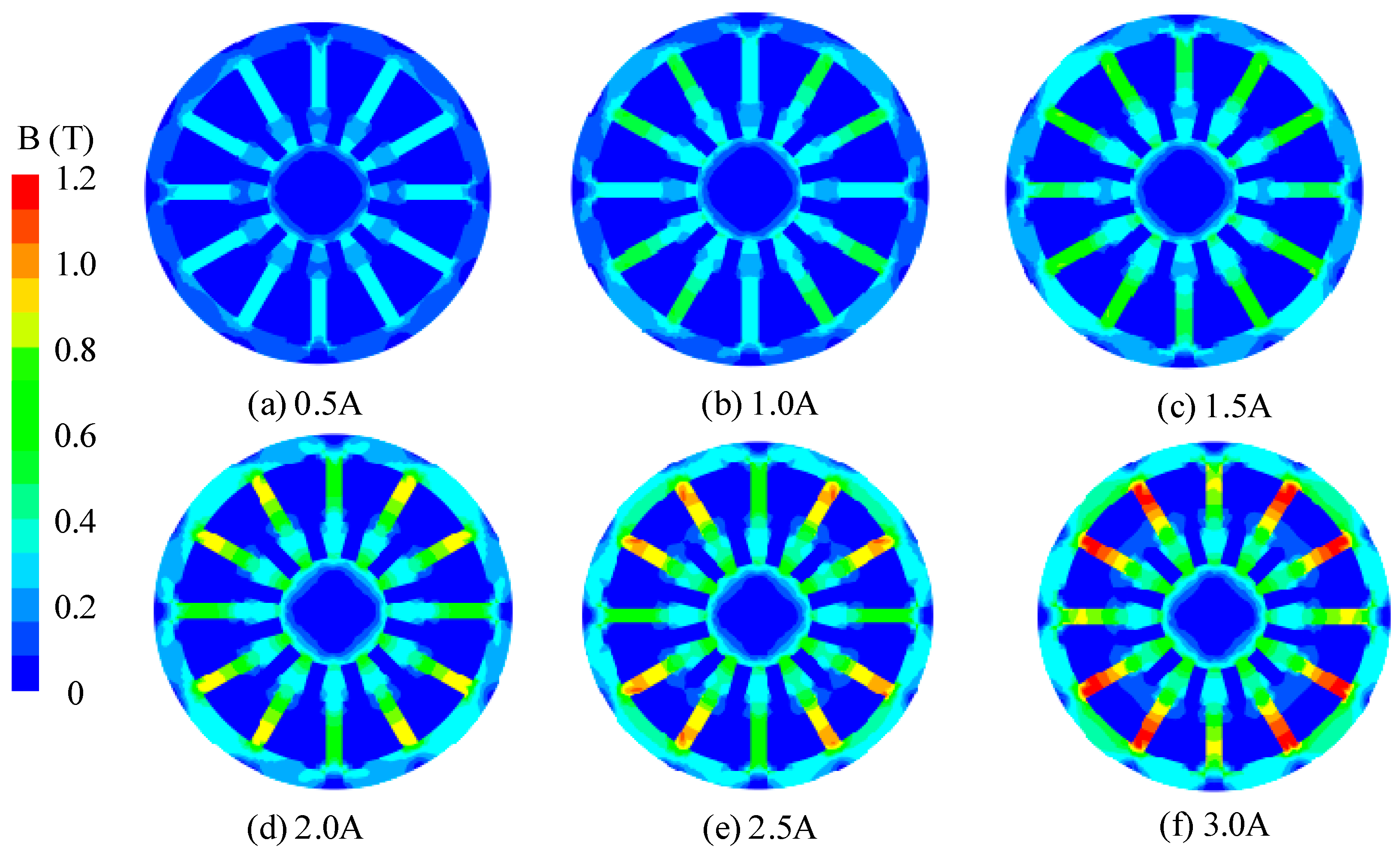
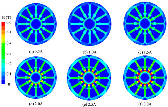
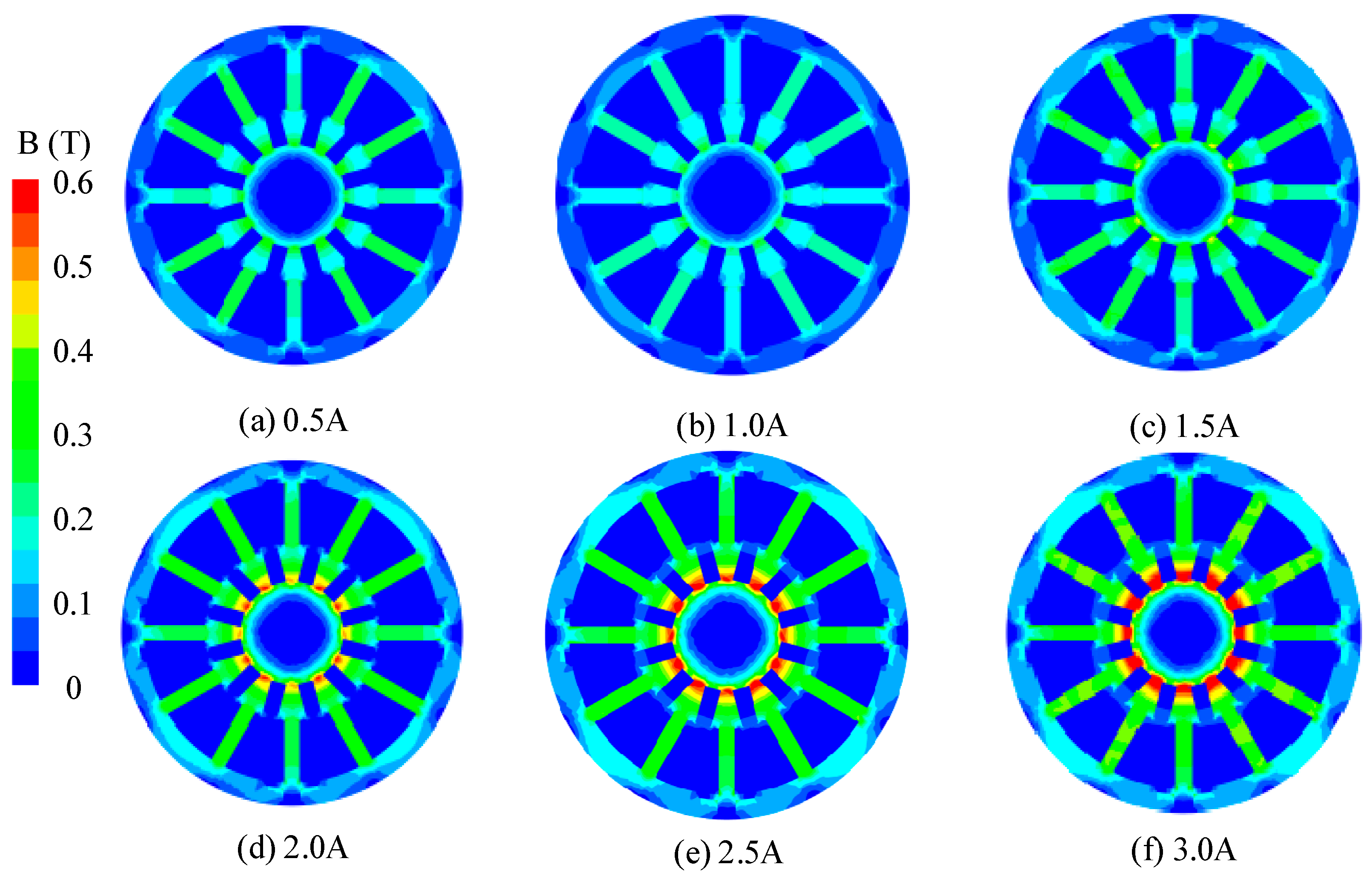
Unlike reverse current, under forward current conditions, the magnetic field directions of the stiffness adjustment coil and the permanent magnet are aligned, resulting in a magnetic flux superposition effect within the working gap. The magnetic induction intensity contour plot shown in Figure 8 indicates that as the forward current increases, the magnetic flux lines gradually concentrate towards the working gap and its adjacent magnetic circuit areas. The magnetic density level within the gap significantly increases, and the range of local high magnetic density areas also expands.
Figure 8.
Distribution gradient of magnetic flux density under different forward currents.
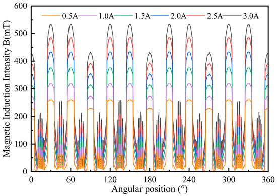
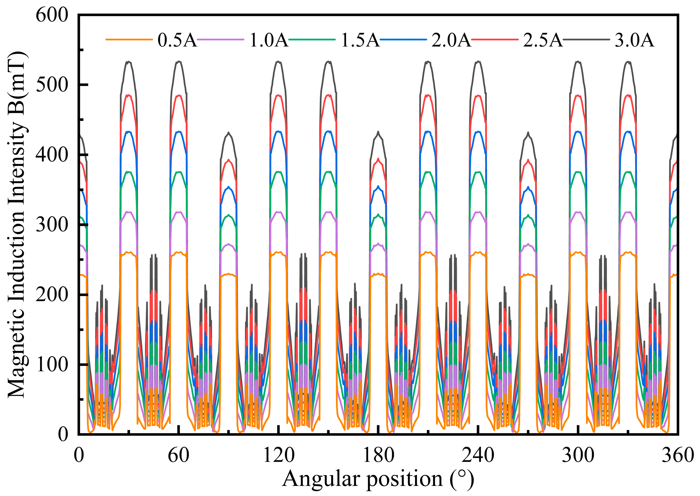
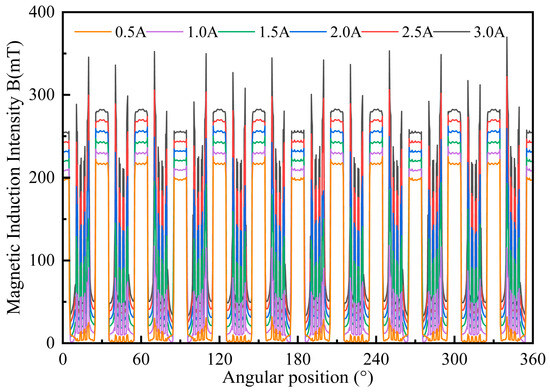
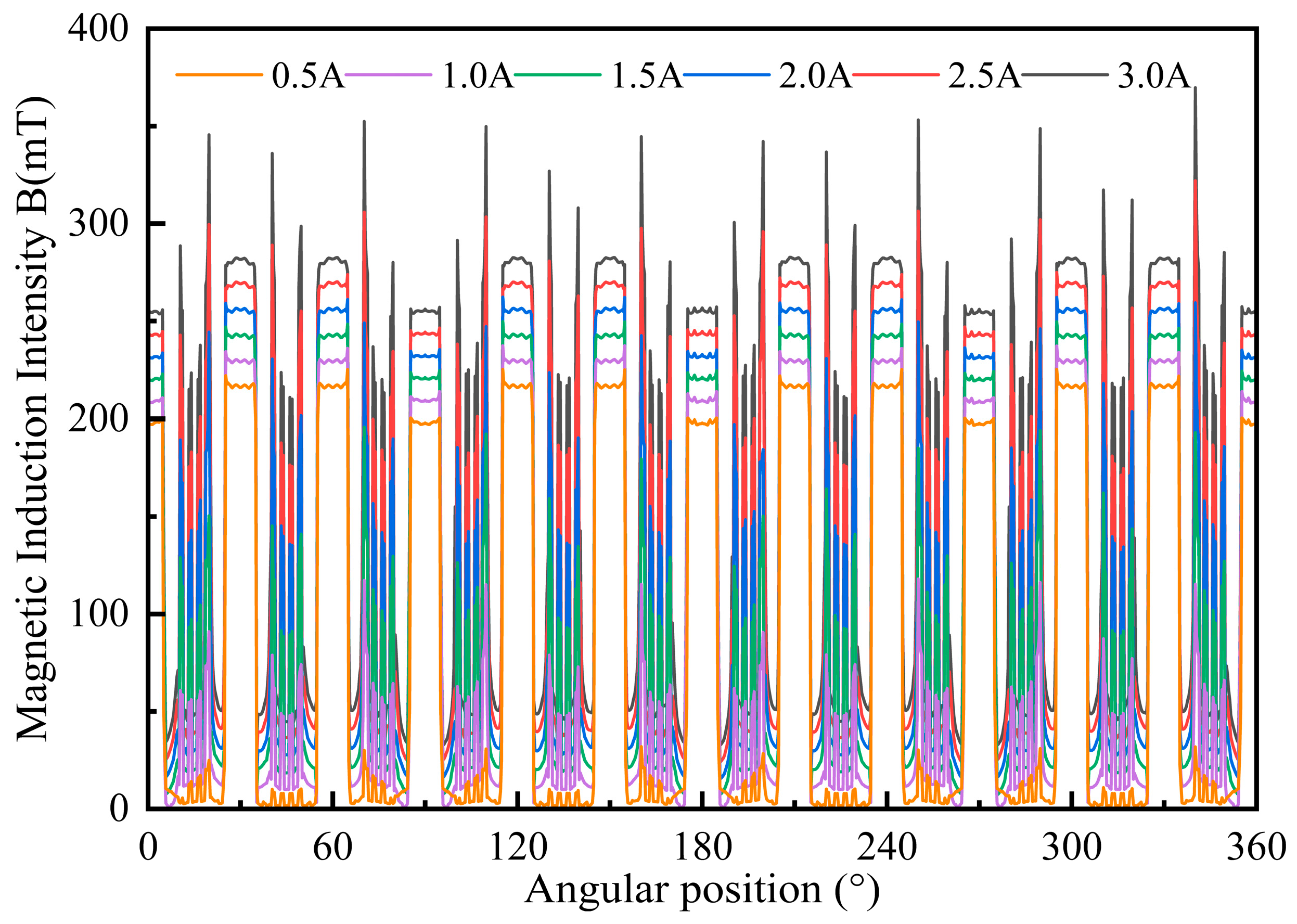
Figure 9 depicts the path curves of magnetic induction intensity in the working gap under different forward currents. The results indicate that as the excitation current increases, the overall curve level gradually shifts upwards, with peak values continuously rising. Moreover, the increase in magnetic induction intensity is more significant in the middle effective working section, indicating that forward excitation can effectively enhance the magnetic field strength in the core area of the gap, thereby improving the magnetization degree of the MR fluid in this region. In contrast, at the four inlet positions of the MR fluid, the magnetic induction intensity is significantly lower than that in the middle working section. The main reason for this is the abrupt change in geometric structure in this area, where magnetic flux diffuses before entering the working gap, leading to magnetic flux leakage and a relatively high equivalent magnetic reluctance. As a consequence, the concentration of magnetic flux is reduced.
Figure 9.
Relationship curve of magnetic flux density with angular position under different forward currents.
The stiffness adjustment coil can regulate the magnetic induction intensity in the working gap within a wide range: reverse excitation weakens the magnetic field to expand the lower limit of stiffness, while forward excitation enhances the magnetic field to increase the upper limit of stiffness, enabling the system to achieve a larger adjustable stiffness range and more flexible operating adaptability. When the reverse current is −1400 A, the average magnetic induction intensity in the working gap decreases to approximately 20 mT; when the forward current is 3.0 A, it increases to approximately 520 mT. The error between the simulation results and the theoretical calculation values is less than 8%, which verifies the accuracy of the equivalent magnetic circuit model.
5.3. Influence of Shaft-Mounted Coil Current on Magnetic Field Distribution
The shaft-mounted coils are arranged on the rotor side, with a total number of 200 turns. Its core function is not to directly enhance the magnetic induction intensity within the working gap of the MR fluid, but rather to excite the rotor core, enabling it to form an adjustable magnetic pole distribution. This, in turn, facilitates electromagnetic coupling with the permanent magnet field on the stator side, generating additional electromagnetic torque and achieving the regulation of output torque.
Figure 10 shows the contour plot of magnetic induction intensity under the influence of different shaft-mounted coil currents. As the excitation current increases, the magnetic flux density inside the rotor significantly increases, with the magnetic flux mainly concentrated in the rotor pole region and forming a closed magnetic circuit with the stator permanent magnet through the working gap. A directional electromagnetic force is generated in the working gap, and the component of this electromagnetic force in the circumferential direction constitutes the driving or braking torque.
Figure 10.
Distribution gradient of magnetic flux density under different shaft-mounted coil currents.
Figure 11 shows the distribution curve of the magnetic induction intensity in the working gap along a specific path. The results show that under different shaft-mounted coil currents, the variation range of magnetic induction intensity in the working gap is relatively limited, the overall curve shape is basically consistent, and only a slight increase occurs in the local region. Because the magnetic field generated by the shaft-mounted coil is mainly concentrated in the rotor, tangential magnetic repulsion force is formed at the pole shoe with the permanent magnet magnetic field, and the radial component of the force is very small, so the radial magnetic field distribution of the working gap is weakly affected, and the stiffness adjustment process will not be disturbed, so the decoupling control of stiffness and torque is realized.
Figure 11.
Relationship curve of magnetic flux density with angular position under different shaft-mounted coil currents.
6. Conclusions
To overcome the limitations of conventional MR fluid hydrostatic bearings, including limited load capacity, insufficient output torque, and poor adaptability to complex operating conditions, a dual-excitation variable-stiffness MR fluid hydrostatic bearing is proposed. This study systematically investigates its structural design, theoretical modeling, and magnetic field simulation. The main conclusions are as follows.
The dual-excitation structure composed of permanent magnets, stiffness adjustment coils and shaft-mounted coils realizes the decoupling control of bearing stiffness and load torque. Radially magnetized permanent magnets provide a stable basic magnetic field to guarantee the fundamental support performance; stiffness adjustment coils achieve wide-range bidirectional stiffness regulation through magnetic field superposition or cancellation with permanent magnets; shaft-mounted coils generate auxiliary driving torque via magnetic repulsion to compensate oil film friction torque and expand the load torque margin. The independent or coordinated control of the two sets of coils enables the bearing to meet multi-dimensional performance requirements under variable load, variable speed and strong disturbance conditions.
Based on the Bingham constitutive model of MR fluid and classical hydrostatic lubrication theory, the mechanistic mathematical models of total stiffness-current and total load torque-current are derived. The equivalent magnetic circuit model is established to calculate and optimize the magnetic resistance of each component, permanent magnet magnetomotive force and coil excitation ampere-turns. Ansys Maxwell 2022 R1 simulation results show that the stiffness adjustment coil can bidirectionally regulate the magnetic induction intensity in the working gap. The shaft-mounted coil mainly affects the rotor magnetic pole distribution and has little direct influence on the gap magnetic field. These results confirm the rationality of the magnetic circuit design and the decoupling control between the two excitation systems. This research breaks through the technical limitation that traditional single-excitation MR hydrostatic bearings can only achieve unidirectional stiffness adjustment, providing a new technical solution for intelligent active control of hydrostatic bearings. The proposed device has the advantages of a wide stiffness adjustment range, fast response and strong working condition adaptability. It shows promising application potential in core support systems of high-end equipment, such as heavy mining machinery spindles and wind turbine main shafts.
To further validate the proposed theoretical model, a dedicated experimental platform is currently under development. The test system includes a prototype MR fluid hydrostatic bearing, torque measurement system, displacement sensing module, and a dual-channel current-controlled excitation system.
The experimental study will focus on verifying the stiffness-current and torque-current relationships under different operating conditions. The results will be reported in subsequent work.
Author Contributions
Conceptualization, H.L. and G.L.; methodology, H.L.; software, Y.B.; validation, H.L., G.L. and S.Z.; formal analysis, H.L. and G.L.; investigation, S.W. (Shumeng Wang); resources, H.L.; data curation, H.L.; writing—original draft preparation, G.L.; writing—review and editing, H.L.; visualization, S.W. (Shuyou Wang); supervision, S.Z.; project administration, H.L.; funding acquisition, H.L. All authors have read and agreed to the published version of the manuscript.
Funding
This work was supported by the National Natural Science Foundation of China (No. 52305078 and 52305064), and China Postdoctoral Science Foundation (No. 2024M751227).
Data Availability Statement
The raw simulation data and finite element models supporting the conclusions of this article are available on request from the corresponding author. No publicly archived datasets were generated within this theoretical and numerical simulation research.
Conflicts of Interest
Author Haopeng Li was employed by the Jiangsu Wuyang Self-Control Technology Co., Ltd. The remaining authors declare that the research was conducted in the absence of any commercial or financial relationships that could be construed as a potential conflict of interest.
References
- Liu, Z.; Wang, Y.; Cai, L.; Zhao, Y.; Cheng, Q.; Dong, X. A review of hydrostatic bearing system: Researches and applications. Adv. Mech. Eng. 2017, 9, 1687814017730536. [Google Scholar] [CrossRef] [Scilit]
- Ueda, H.; Saito, M.; Kawamura, Y.; Kawada, S.; Miyatake, M. Study on static and dynamic characteristics of water-lubricated hydrostatic thrust bearings—Effect of feed hole inlet shape on bearing characteristics. Tribol. Int. 2024, 191, 109127. [Google Scholar] [CrossRef] [Scilit]
- Li, R.; He, X.; Zhang, K.; Peng, Y.; Zhan, D. Analysis of the hydrodynamic effect on the load capacity and rotational accuracy of hydrostatic spindle. Ind. Lubr. Tribol. 2025, 77, 1113–1122. [Google Scholar] [CrossRef] [Scilit]
- Lin, S.Y.; Jiang, S.Y. Rotordynamics of an Improved Face-Grinding Spindle: Rotational Stiffness of Thrust Bearing Increases Radial Stiffness of Spindle. J. Manuf. Sci. Eng.-Trans. ASME 2022, 144, 084502. [Google Scholar] [CrossRef] [Scilit]
- Yu, X.; Wang, F.; Zhou, D.; Huang, D.; Zhan, S.; Yu, M.; Jiao, J.; Wang, J. Deformation characteristics of adaptive hydrostatic thrust bearing under extreme working conditions. J. Braz. Soc. Mech. Sci. Eng. 2020, 42, 489. [Google Scholar] [CrossRef] [Scilit]
- Quinci, F.; Litwin, W.; Wodtke, M.; Nieuwendijk, R.v.D. A comparative performance assessment of a hydrodynamic journal bearing lubricated with oil and magnetorheological fluid. Tribol. Int. 2021, 162, 107143. [Google Scholar] [CrossRef] [Scilit]
- Rehman, W.U.; Wang, X.; Cheng, Y.; Chen, Y.; Shahzad, H.; Chai, H.; Abbas, K.; Ullah, Z.; Kanwal, M. Model-Based Design Approach to Improve Performance Characteristics of Hydrostatic Bearing Using Multivariable Optimization. Mathematics 2021, 9, 388. [Google Scholar] [CrossRef] [Scilit]
- Wodtke, M.; Litwin, W.; Van Der Meer, G.; Van Ostayen, R. Wear tests of hydrodynamic journal bearings lubricated with magnetorheological fluid. Wear 2026, 584–585, 206404. [Google Scholar] [CrossRef] [Scilit]
- Ahn, K.K.; Truong, D.Q.; Islam, M.A. Modeling of a magneto-rheological (MR) fluid damper using a self tuning fuzzy mechanism. J. Mech. Sci. Technol. 2009, 23, 1485–1499. [Google Scholar] [CrossRef] [Scilit]
- Wu, X.; Guo, Y.; Tian, Z.; Li, H.; Shi, Z. Preparation and Performance Evaluation of a High Temperature Stable Magnetorheological Fluid with Shear-Thinning Resistance. Materials 2025, 18, 3840. [Google Scholar] [CrossRef] [Scilit] [PubMed]
- Wang, N.; Liu, X.; Sun, S.; Krolczyk, G.; Li, Z.; Li, W. Microscopic characteristics of magnetorheological fluids subjected to magnetic fields. J. Magn. Magn. Mater. 2020, 501, 166443. [Google Scholar] [CrossRef] [Scilit]
- Hesselbach, J.; Abel-Keilhack, C. Active hydrostatic bearing with magnetorheological fluid. J. Appl. Phys. 2003, 93, 8441–8443. [Google Scholar] [CrossRef] [Scilit]
- Rouabah, S.; Didouche, F.Y.; Khebli, A.; Aguib, S.; Chikh, N. The Advancing Understanding of Magnetorheological Fluids and Elastomers: A Comparative Review Analyzing Mechanical and Viscoelastic Properties. Magnetochemistry 2025, 11, 62. [Google Scholar] [CrossRef] [Scilit]
- Ma, L.; Mu, L.; Lan, W.; Li, P.; Wang, J.; Qin, Z.; Chu, F. Nonlinear characteristics of a magnetorheological bearing-rotor system. Appl. Math. Mech.-Engl. Ed. 2026, 47, 77–98. [Google Scholar] [CrossRef] [Scilit]
- Maurya, C.S.; Sarkar, C. Magnetorheological fluids: A comprehensive review of operational modes and performance under varied circumstances. Rheol. Acta 2024, 63, 765–785. [Google Scholar] [CrossRef] [Scilit]
- Wang, X.; Li, H.; Lu, W.; Meng, G. Stiffness and Damping Properties of (Semi) Floating Ring Bearing Using Magnetorheological Fluids as Lubricant. J. Tribol.-Trans. ASME 2017, 139, 051701. [Google Scholar] [CrossRef] [Scilit]
- Tomar, A.K.; Sharma, S.C.; Sahu, K. Performance Analysis of Textured Spherical Hybrid Journal Bearings Operated With Magnetorheological Fluid. J. Tribol.-Trans. ASME 2024, 146, 014602. [Google Scholar] [CrossRef] [Scilit]
- Gertzos, K.P.; Nikolakopoulos, P.G.; Papadopoulos, C.A. CFD analysis of journal bearing hydrodynamic lubrication by Bingham lubricant. Tribol. Int. 2008, 41, 1190–1204. [Google Scholar] [CrossRef] [Scilit]
- Bompos, D.A.; Nikolakopoulos, P.G. CFD simulation of magnetorheological fluid journal bearings. Simul. Model. Pract. Theory 2011, 19, 1035–1060. [Google Scholar] [CrossRef] [Scilit]
- Wang, X.; Li, H.; Li, M.; Bai, H.; Meng, G.; Zhang, H. Dynamic characteristics of magnetorheological fluid lubricated journal bearing and its application to rotor vibration control. J. Vibroeng. 2015, 17, 1912–1928. [Google Scholar] [CrossRef] [Scilit]
- Osman, T.A.; Nada, G.S.; Safar, Z.S. Effect of using current-carrying-wire models in the design of hydrodynamic journal bearings lubricated with ferrofluid. Tribol. Lett. 2001, 11, 61–70. [Google Scholar] [CrossRef] [Scilit]
- Jing, Z.; Sun, S.; Ouyang, Y.; Zhang, S.; Li, W.; Zheng, J. Design and modeling analysis of a changeable stiffness robotic leg working with magnetorheological technology. J. Intell. Mater. Syst. Struct. 2018, 29, 3725–3736. [Google Scholar] [CrossRef] [Scilit]
- Peng, L.; Hua, D.; Liu, X.; Andriukaitis, D.; Królczyk, G.; Li, Z. Research on control strategy of an active magnetorheological fluid bearing based on improved gray wolf optimization approach. J. Low Freq. Noise Vib. Act. Control 2023, 42, 1821–1836. [Google Scholar] [CrossRef] [Scilit]
- Zhang, H.; Ma, W.; Peng, B.; Feng, K. A novel squeeze mode magnetorheological fluid damper for gas-lubricated journal bearing: Theoretical and experimental investigations. Proc. Inst. Mech. Eng. Part C-J. Mech. Eng. Sci. 2026, 240, 2565–2585. [Google Scholar] [CrossRef] [Scilit]
- Lampaert, S.G.E.; Van Ostayen, R.A.J. Load and stiffness of a hydrostatic bearing lubricated with a Bingham plastic fluid. J. Intell. Mater. Syst. Struct. 2019, 30, 3056–3065. [Google Scholar] [CrossRef] [Scilit]
- Urreta, H.; Leicht, Z.; Sanchez, A.; Agirre, A.; Kuzhir, P.; Magnac, G. Hydrodynamic Bearing Lubricated with Magnetic Fluids. J. Intell. Mater. Syst. Struct. 2010, 21, 1491–1499. [Google Scholar]
- Bompos, D.A.; Nikolakopoulos, P.G. Experimental and analytical investigations of dynamic characteristics of magnetorheological and nanomagnetorheological fluid film journal bearing. J. Vib. Acoust.-Trans. ASME 2016, 138, 031012. [Google Scholar] [CrossRef] [Scilit]
- Van Der Meer, G.; Van Ostayen, R. Investigating Film Thickness and Friction of an MR-Lubricated Journal Bearing. Lubricants 2025, 13, 171. [Google Scholar] [CrossRef] [Scilit]
- Lampaert, S.G.E.; Van Ostayen, R.A.J. Experimental results on a hydrostatic bearing lubricated with a magnetorheological fluid. Curr. Appl. Phys. 2019, 19, 1441–1448. [Google Scholar] [CrossRef] [Scilit]

Disclaimer/Publisher’s Note: The statements, opinions and data contained in all publications are solely those of the individual author(s) and contributor(s) and not of MDPI and/or the editor(s). MDPI and/or the editor(s) disclaim responsibility for any injury to people or property resulting from any ideas, methods, instructions or products referred to in the content. |
© 2026 by the authors. Licensee MDPI, Basel, Switzerland. This article is an open access article distributed under the terms and conditions of the Creative Commons Attribution (CC BY) license.