


Abstract
Reliable identification of drill-string–wellbore friction is important for evaluating mechanical load transfer and contact behavior during drilling. However, friction estimation from surface hook-load measurements can be affected by non-frictional contributions from the hoisting system and drilling-fluid-induced forces. This study develops a multi-physics hook-load correction framework incorporating sheave efficiency, traveling-block and hook weight, mud-hose catenary force, drilling-line weight, annular and internal viscous forces, swab/surge effects, and pump-on hydraulic lift. Field data from a 3500 m directional well were analyzed using a yield-power-law (YPL)/Herschel–Bulkley fluid model. For representative slide- and rotary-drilling intervals, measured average hook loads of 442.21 and 481.01 kN were corrected to 294.92 and 332.89 kN, corresponding to correction ratios of 33.31% and 30.79%. Corrected off-bottom hook loads were then used to identify state-dependent effective drill-string–wellbore friction factors of 0.180, 0.154, and 0.104 at three calibration states. These factors were transferred to subsequent drilling intervals for surface-torque reconstruction. After one-point baseline alignment, the remaining torque samples yielded mean relative reconstruction errors of 2.28%, 4.22%, and 3.21%, respectively. Removing these non-frictional contributions allows the effective drill-string–wellbore friction factor to be identified from a corrected surface load and subsequently compared with the measured torque response.
1. Introduction
Hook load is an important surface parameter reflecting the force state of the drill string during drilling operations. It is closely related to the suspended weight of the drill string, weight-on-bit transmission, drill-string motion, and downhole frictional resistance. Therefore, accurate interpretation of hook load is essential for monitoring downhole conditions, evaluating weight-on-bit, identifying abnormal drilling states, and preventing drilling problems such as excessive drag, poor weight transfer, and stuck-pipe incidents [1,2]. Previous studies have shown that surface parameters such as hook load and rotary torque can be used for real-time drilling-condition analysis and key-parameter prediction. Reliable hook-load interpretation can also provide an important basis for wellbore-cleaning evaluation and drilling-risk diagnosis, thereby reducing non-productive time (NPT) and associated economic losses [3].
However, the hook load measured at the surface does not always represent the actual suspended load of the drill string. In field operations, the hook load is usually obtained indirectly from the deadline sensor or the surface hoisting system. The measured value is affected not only by the buoyed weight of the drill string and the friction between the drill string and the wellbore, but also by several surface mechanical and hydraulic factors. Mechanical losses in the surface hoisting system, including pulley friction, traveling block and hook weight, drilling-line weight, and the mud-hose catenary effect, may introduce systematic deviations into the measured hook-load signal. In addition, under pump-on circulation and drill-string movement, fluid viscous forces, swab/surge effects, and pump-on hydraulic lift force can further change the apparent hook-load response. If these factors are neglected, the calculated hook load may deviate significantly from the true load acting on the drill string.
Many studies have been carried out to improve the understanding and correction of hook-load measurements. In terms of surface mechanical correction, Luke and Juvkam-Wold [4] investigated the influence of sheave friction on the hoisting system through theoretical derivation and experimental verification. Their results showed that pulley friction causes the tensions in different drilling-line sections to follow a geometric progression, and the relationship between deadline tension and actual hook load depends on the motion direction of the traveling block. Based on this mechanism, they established a dynamic correction model for hook load considering traveling-block motion direction and pulley efficiency, which provided an important theoretical basis for correcting errors caused by the hoisting system. Cayeux et al. [5] further analyzed the error sources of hook-load measurement using the deadline method. They considered the influence of surface equipment, including pulley efficiency, mud-hose catenary effect, and top-drive carriage movement, and developed a mathematical correction model to reduce measurement deviations caused by surface mechanical factors.
In addition to surface mechanical effects, drilling-fluid-related forces also play an important role in hook-load interpretation. During pump-on circulation, drilling fluid flows downward inside the drill string and returns upward through the annulus. The viscous shear stress generated along the inner and outer surfaces of the drill string produces axial fluid forces, which may increase or decrease the apparent hook load depending on the flow direction and operating condition. Hamidov et al. [6] established a comprehensive hook-load prediction model coupled with fluid dynamics. By introducing viscous friction and pump-on hydraulic force terms based on the YPL rheological model, their model improved the correction of hook-load deviations caused by fluid viscous resistance and hydraulic effects.
The calculation of fluid-induced forces depends strongly on the rheological characteristics of drilling fluids. For non-Newtonian drilling fluids, the Herschel–Bulkley or yield-power-law (YPL) model is commonly used to describe yield stress and shear-thinning behavior. Kelessidis et al. [7] proposed an optimal method for determining Herschel–Bulkley rheological parameters and demonstrated that these parameters have a significant influence on pressure drop and velocity profiles during drilling. Founargiotakis et al. [8] presented an integrated calculation approach for Herschel–Bulkley fluid flow in concentric annuli, covering laminar, transitional, and turbulent flow regimes. These studies provide useful theoretical support for calculating annular and internal pressure losses of non-Newtonian drilling fluids.
Swab and surge effects are another important source of hook-load variation during drill-string movement. When the drill string moves upward or downward in a wellbore filled with drilling fluid, the relative motion between the pipe and the fluid can generate additional pressure differences in the annulus. These pressure differences act on the effective cross-sectional area near the bit and generate additional axial forces. Belimane et al. [9] developed a numerical model for surge pressure during tripping operations in eccentric annuli and showed that annular eccentricity affects velocity distribution and apparent viscosity distribution. Their work indicates that swab/surge pressure is closely related to annular geometry, drilling-fluid rheology, and pipe movement velocity, and should be considered when correcting hook load under tripping or pipe movement conditions.
Data-driven methods have also been applied to hook-load and surface-parameter prediction. Song et al. [2] proposed a BP-LSTM dual-input network to predict hook load and rotary drive torque, showing that machine-learning methods can capture nonlinear relationships among drilling parameters and surface mechanical responses. Such methods are useful for real-time prediction and trend tracking when sufficient field data are available. Nevertheless, purely data-driven approaches usually depend on the quality and representativeness of training samples, and their mechanical interpretability may be limited when operating conditions change. Therefore, physics-based correction models remain necessary for interpreting the underlying force mechanisms and improving the physical reliability of measured hook-load data under varying operating conditions.
Classical torque-and-drag models provide a physics-based framework for relating surface axial load and rotary torque to drill-string–wellbore contact and friction. Johancsik et al. [10] established a classical soft-string model in which torque and drag are primarily attributed to sliding friction generated by the normal contact force. Sheppard et al. [11] further extended the analytical treatment for evaluating the influence of wellbore trajectory on drill-string torque and drag. Brett et al. [12] demonstrated that drill-string tension and torque models can be combined with field measurements for drilling-condition monitoring, while Reiber et al. [13] introduced real-time torque-and-drag analysis for drilling-performance evaluation. Aadnøy and Andersen [14] developed analytical friction equations applicable to straight and curved well sections, three-dimensional well trajectories, and combined axial and rotational motion. Subsequent studies further generalized these formulations for different wellbore geometries and drilling modes [15,16,17]. Mitchell and Samuel [18] evaluated the assumptions and limitations of conventional soft-string torque-and-drag models. These studies provide the theoretical basis for relating drill-string–wellbore friction to both axial load and rotary torque, thereby enabling the friction state inferred from corrected hook load to be further examined through the torque response.
Drill-string–wellbore friction is affected by both the normal contact load and the relative motion at the interface. Wellbore curvature changes the contact force, whereas simultaneous axial motion and rotation determine how the available friction force is distributed between the axial and circumferential directions [14,15,16,17]. Drilling fluid is also present in the contact region and can modify the friction and wear response of the contacting surfaces. Experimental studies have shown that the base fluid, lubricant additives, temperature, suspended solids, and interfacial films can significantly affect the coefficient of friction and wear behavior [19,20,21,22,23]. Reviews of water-based drilling-fluid lubricants further indicate that the measured friction response depends on lubricant chemistry and operating/contact conditions [24,25].
Previous studies have established important methods for individual components of this problem. Luke and Juvkam-Wold [4] and Cayeux et al. [5] addressed hook-load estimation and correction associated with the surface hoisting system, while Hamidov et al. [6] incorporated fluid-flow-related forces and hydraulic effects into torque-and-drag calculations. Classical torque-and-drag models, including that of Johancsik et al. [10], provide established approaches for friction-factor-based prediction of axial load and torque. Building on these contributions, the present study focuses on the workflow connecting condition-dependent corrections to measured hook load with effective friction-factor identification from corrected off-bottom loads and subsequent torque-response consistency assessment. The contribution is therefore methodological and application-oriented, rather than the proposal of a new constitutive friction law or a new model for each individual correction term. Specifically, the study integrates condition-dependent, signed corrections for relevant surface-mechanical and fluid-induced contributions to the measured hook load. The corrected off-bottom hook load is then used as the axial-load target for identifying a state-dependent effective drill-string–wellbore friction factor. The identified factor is subsequently applied to selected later drilling intervals, where the calculated surface-torque response is compared with field measurements after baseline alignment. This comparison provides a supplementary assessment of short-term consistency between the corrected-load-based friction identification and the measured torque response. The workflow is demonstrated using field data from a single 3500 m directional well. Further applications of this workflow to additional wells and operating conditions are needed to assess its broader transferability.
2. Materials and Methods
2.1. Overall Correction Framework
The hook load recorded by the surface deadline sensor does not directly represent the axial load carried by the drill string at the wellhead. In addition to the drill-string load, the measured signal contains contributions from the surface hoisting system and drilling-fluid-induced forces. The magnitude and direction of these contributions vary with the operating conditions. Therefore, the measured hook load is corrected by separately evaluating the surface mechanical and fluid-dynamic effects.
The overall correction can be expressed as:
where HLm is the measured hook load, HLc is the corrected hook load representing the axial load of the drill string at the wellhead, and ∆HLmech and ∆HLfluid are the signed corrections associated with the surface mechanical system and fluid-dynamic effects, respectively.
HLc = HLm + △HLmech + △HLfluid
Throughout this study, all ∆HL terms are defined as signed corrections that are added algebraically to the measured hook load. A positive correction increases HLc relative to HLm, whereas a negative correction decreases it. The sign of a motion-dependent correction is not prescribed universally but is determined from the actual drill-string motion direction and the corresponding force direction. Thus, the same physical mechanism may produce corrections of opposite signs during pick-up and slack-off operations.
The surface mechanical correction is written as
where ∆HLsheave, ∆HLtb, ∆HLhose, and ∆HLline are the signed corrections associated with sheave-system transmission efficiency, the self-weight of the traveling block and hook assembly, the mud-hose effect, and the self-weight of the drilling line, respectively. Among these terms, the sheave-system correction is explicitly dependent on the direction of load transmission and is therefore evaluated separately for pick-up and slack-off operations.
△HLmech = △HLsheave + △HLtb + △HLhose + △HLline
The fluid-dynamic correction is expressed as
where ∆HLann, ∆HLint, ∆HLss, and ∆HLlift denote the signed corrections associated with annular viscous force, internal viscous force, swab/surge-induced axial force, and pump-on hydraulic lift, respectively. Buoyancy is treated separately through the buoyancy factor when evaluating the effective drill-string weight in the subsequent torque-and-drag model.
△HLfluid = △HLann + △HLint + △HLss + △HLlift
The active correction components depend on the operating conditions. For example, circulation-related viscous and hydraulic terms are active during pump-on drilling, whereas the swab/surge contribution becomes important when appreciable axial pipe motion occurs. The direction of the annular and internal viscous forces also depends on the relative motion between the drilling fluid and the drill string. Therefore, the individual correction components are evaluated separately before being assembled through Equations (1)–(3).
In this study, the corrected hook load refers specifically to the corrected axial load carried by the drill string at the wellhead and is not treated as a direct measurement of downhole weight on bit. The corrected hook load is subsequently used as the calibration target for identifying an effective friction factor. The identified friction factor is then introduced into the torque-and-drag model to calculate the friction-related torque response. Because the measured surface torque is not involved in either the hook-load correction or the friction-factor identification, it is subsequently used for one-point baseline-aligned surface-torque reconstruction and consistency assessment, as described in Section 2.7 and Section 3.2.
2.2. Surface Mechanical Correction
The surface mechanical correction quantifies the systematic load deviations introduced by the hoisting and suspended-equipment system. For a deadline-based hook-load measurement, the recorded load is influenced by the transmission efficiency of the sheave system, the self-weight of the traveling block and hook assembly, the vertical force exerted by the mud hose, and the self-weight of the drilling line. These contributions do not represent the axial load carried by the drill string and therefore need to be accounted for before the measured hook load is interpreted as the wellhead drill-string load. The corresponding correction terms are formulated separately in the following subsections.
2.2.1. Sheave-System Efficiency Correction
Sheave friction is one of the primary sources of systematic error in deadline-based hook-load measurements. Because mechanical energy is dissipated at each sheave, the rope tension changes progressively as the drilling line passes through the crown-block and traveling-block sheaves. Consequently, the tension measured at the deadline does not directly equal the load supported by the traveling system. The magnitude and direction of this deviation depend on the direction of load transmission and the operating state of the traveling block. During pick-up and slack-off operations, the sheave friction acts in opposite directions and therefore must be treated separately [4,26].
Active Deadline Sheave. When the deadline sheave rotates and its frictional effect is included, the rope tension changes as the drilling line passes through the first sheave, as illustrated in Figure 1.
Figure 1.
Active deadline sheave.
For the reeving arrangement considered here, the line segment adjacent to the deadline sensor is taken as the reference segment. When the deadline-side sheave is active, the tension transmitted from the measured deadline segment to the first supporting line is determined by the single-sheave efficiency.
For an active deadline sheave, during pick-up operations:
For an active deadline sheave, during slack-off operations:,
Inactive Deadline Sheave. Assuming that the deadline sheave remains stationary and that frictional loss can be neglected, the first line tension is equal to the deadline tension, while it corresponds to the fast-line tension [27], as illustrated in Figure 2.
Figure 2.
Inactive deadline sheave.
For an inactive deadline sheave, during pick-up operations:
For an inactive deadline sheave, during slack-off operations:
where HLeq is the equivalent hook load inferred from the deadline tension after accounting for the sheave-efficiency and reeving relationship, Fdl is the reading of the load sensor installed at the deadline end, n is the number of drilling lines, and e is the efficiency of a single sheave.
In the present rig configuration, the deadline end is fixed to the rig floor, and the line segment connected to the deadline sensor is assumed not to undergo appreciable translational motion during the selected operating intervals. Based on the adopted reeving arrangement, the deadline-side sheave is therefore treated as stationary for the present calculation, and frictional loss at this sheave is neglected. This treatment is a boundary-condition assumption specific to the investigated hoisting-system configuration and should not be interpreted as universally applicable to all rig arrangements.
2.2.2. Traveling Block and Hook Assembly Correction
The load transmitted through the traveling system includes not only the suspended drill-string load but also the self-weight of the traveling block and hook assembly. If the field hook-load signal includes this equipment weight, it must be removed when the objective is to determine the axial load carried by the drill string. The corresponding equipment weight is calculated as
where mtb is the mass of the traveling block and hook assembly and g is gravitational acceleration. The corresponding signed hook-load correction is
when the equipment weight is included in the measured hook-load signal. For the field case considered in this study, mtb = 15 t corresponding to
Wtb = mtbg
△HLtb = −Wtb
Wtb = 147.15 kN
2.2.3. Mud-Hose Catenary Correction
In a top-drive drilling system, the high-pressure mud hose connects the fixed standpipe manifold to the vertically moving top drive. Unlike the rigid components of the hoisting system, the hose forms a flexible suspended structure, and its weight is shared between the standpipe support and the top-drive connection. As the traveling system moves vertically, the suspended configuration of the hose varies continuously, resulting in a redistribution of the load transmitted to the top drive. Consequently, the vertical force exerted by the mud hose constitutes an additional contribution to the surface hook-load measurement and should be considered in the mechanical correction.
To quantify this effect, the mud hose is modeled as a homogeneous flexible cable with constant linear mass density. The elastic elongation of the hose under operating pressure is assumed to be negligible relative to its total length; therefore, the hose is treated as an inextensible catenary subjected primarily to gravity [28,29]. The corresponding geometric and force parameters are illustrated in Figure 3.
Figure 3.
Schematic force model of the mud-hose effect on the traveling system.
A local coordinate system is introduced with its origin located at the lowest point of the catenary, where x and y denote the horizontal and vertical coordinates, respectively. The catenary profile is expressed as:
where a is the catenary parameter.
Let x1 and x2 denote the horizontal coordinates of the top-drive-side and standpipe-side suspension points, respectively, and let htd and hsp denote their corresponding elevations. If x1 is the coordinate of the top-drive-side suspension point, the standpipe-side coordinate is:
x2 = x1 + d
The geometric boundary conditions of the suspended hose can then be written as
By simultaneously solving these two nonlinear equations, the catenary parameter a and the suspension-point coordinate x1 can be determined for a given position of the traveling system. The top-drive-side coordinate x2 is then obtained from x2 = x1 + d.
The horizontal component of the catenary tension is related to the catenary parameter by
where λmh is the combined linear mass density of the mud hose and the drilling fluid contained inside the hose, and g is gravitational acceleration. Accordingly, the vertical component of the hose tension acting at the top-drive connection, Tv, is defined as:
Th = aλmhg
The mud hose pulls the top-drive connection toward the suspended hose. For the configuration shown in Figure 3, the vertical component of this force acts downward on the top-drive assembly and, therefore, increases the load carried by the traveling system. Since this contribution does not belong to the axial load carried by the drill string, it is removed from the measured hook load. In the signed correction framework defined in Section 2.1, the mud-hose correction is, therefore, expressed as
when the positive hook-load direction is defined as downward load carried by the traveling system.
△HLhose = −Tv
The horizontal component mainly acts on the top-drive guide system and does not directly contribute to the axial hook load. However, it may introduce a small additional axial force through friction between the top drive and the guide rails. In the present study, this possible contribution was estimated conservatively from the calculated horizontal mud-hose tension and was found to be small relative to the hook load under the investigated operating conditions. A quantitative evaluation of this assumption is provided, together with the correction results, in Section 3.1. Therefore, only the vertical component of the mud-hose tension is included in the present hook-load correction.
2.2.4. Drilling-Line Weight Correction
The self-weight of the drilling line introduces an additional contribution to the tension measured at the deadline. This effect becomes particularly relevant when the actual drill-string hook load is relatively low, because the drilling-line weight then accounts for a larger proportion of the total measured load. Moreover, the cumulative effect increases with the number of supporting lines in the hoisting system [30]. Therefore, the gravitational contribution of the drilling line is explicitly included in the surface mechanical correction. The force analysis for this term is illustrated in Figure 4.
Figure 4.
Mechanical model of the drilling-line self-weight effect on hook load.
In Figure 4, the suspended length of each drilling-line segment between the crown block and traveling block varies with traveling-block position. The drilling-line weight model is derived under quasi-static conditions. The supporting line segments between the crown block and traveling block are approximated as vertical, the drilling line is assumed to have a uniform linear mass density, and elastic deformation and dynamic inertia are neglected. The relationship between the tensions on the two sides of the relevant sheaves can then be expressed as follows:
Similarly, the relationship between the tension T2i+1 on the right side of sheave B2i+1 and the tension T2i on the left side of sheave B2i, which belongs to the traveling block, can be expressed as follows:
Forces acting on the traveling equipment and the derrick: the total tension exerted by the supporting lines on the traveling equipment is given by:
The self-weight of the drilling line exerts a downward force on the traveling equipment and, therefore, contributes to the deadline-sensor reading. This contribution must be removed when the objective is to obtain the axial load carried by the drill string. Although the drilling-line mass density is constant, the suspended line-weight contribution varies with traveling-block position because the suspended line length changes during operation. Its relative contribution generally decreases as the drill-string suspended load increases, although the correction magnitude should always be evaluated from the actual hoisting-system geometry and operating state.
This mechanically corrected load is subsequently combined with the fluid-dynamic corrections described in Section 2.3 to obtain the final corrected hook load.
2.3. Fluid-Dynamic Correction Model
In addition to the surface mechanical effects described in Section 2.2, the wellhead axial load is influenced by fluid-induced forces associated with viscous shear along the inner and outer pipe surfaces, swab/surge pressure, and the pressure imbalance generated during pump-on circulation. These forces may either increase or decrease the apparent hook load depending on the circulation direction, drill-string motion, and relative velocity between the pipe and drilling fluid. Therefore, the fluid-dynamic correction is formulated using signed force components rather than fixed algebraic directions.
The total fluid-dynamic correction is expressed as:
where the terms on the right-hand side denote the contributions of annular viscous force, internal viscous force, swab/surge-induced axial force, and pump-on hydraulic lift, respectively. The magnitude and sign of each term are evaluated according to the corresponding operating conditions. Buoyancy is not included as an independent signed hook-load correction term; it is treated separately through the buoyancy factor when evaluating the effective drill-string weight in the subsequent torque-and-drag model.
△HLfluid=△HLann+△HLint+△HLss+△HLlift
2.3.1. Buoyancy Treatment for the Subsequent Mechanical Model
When the drill string is immersed in drilling fluid, its effective gravitational weight is reduced by buoyancy. Figure 5 schematically illustrates the gravity and buoyancy acting on an immersed drill-string element. In the present study, buoyancy is not treated as an independent signed hook-load correction term because the wellhead axial load carried by the drill string under downhole conditions already reflects the effect of buoyancy. Instead, the buoyancy factor is introduced only to evaluate the effective drill-string weight used in the subsequent torque-and-drag model.
Figure 5.
Forces acting on an unrestricted drill string submerged in drilling fluid in a vertical well.
For a drill-string element with length ΔL, the in-air weight can be expressed as
where ρs is the drill-string material density, As is the steel cross-sectional area, g is gravitational acceleration, and ΔL is the element length.
Wair = ρsAsg△L
The effect of drilling-fluid buoyancy is represented by the buoyancy factor:
where ρm is the drilling-fluid density. The corresponding buoyed weight is
Wb = βWair
2.3.2. Annular and Internal Fluid Viscous Forces
During pump-on circulation, drilling fluid flows downward through the drill string and returns upward through the annulus. Relative motion between the drilling fluid and the pipe walls generates viscous shear stresses on both the internal and external surfaces of the drill string. These shear stresses produce additional axial forces and therefore modify the hook-load response.
As illustrated in Figure 6, the internal drilling fluid generally flows downward and exerts a downward viscous force on the inner wall of the drill string, whereas the annular return flow moves upward and exerts an upward viscous force on the external pipe surface. The two contributions act in opposite directions and must therefore be evaluated separately before being algebraically combined according to the actual operating conditions.
Figure 6.
Schematic of fluid flow inside and outside the drill string.
Considering the viscous pressure-drop contribution and the additional inertial effect associated with curved flow paths, the axial fluid force can be expressed in the general form as
where Cτo is the annular geometric correction coefficient, φo denotes the frictional pressure-drop contribution in the annulus, A is the corresponding cross-sectional area, ρ and v are the drilling-fluid density and average velocity, respectively, and the subscripts o and i denote the annular and internal flow regions.
The general formulation also contains an inertial contribution associated with fluid motion through curved well sections. An order-of-magnitude assessment shows that, under the drilling flow rates and dogleg severities considered in this study, this term is considerably smaller than the viscous pressure-drop contribution to the axial hook-load response. Therefore, only the viscous pressure-drop term is retained in the subsequent hook-load correction, while the higher-order inertial contribution is neglected.
To account for the geometric asymmetry of the annular flow passage, the correction coefficient proposed by Mitchell [31] is introduced. For internal circular-pipe flow, the corresponding coefficient is unity, whereas for annular flow, the correction coefficient is expressed as
where Dh is the borehole diameter, and Do is the outer diameter of the pipe.
The frictional pressure-drop terms for the annular and internal flow regions are determined using the YPL/Herschel–Bulkley rheological model, which accounts for the yield-stress and shear-thinning behavior [7,32] of the drilling fluid:
where τ is the shear stress, τy is the yield stress, K is the consistency index, nf is the flow-behavior index, and is the shear rate. Compared with a Newtonian approximation, this model provides a more appropriate description of the rheological behavior of the drilling fluid used in the present well.
Annular flow. The average annular return velocity is determined from the circulating flow rate and the available annular flow area:
where
Dh is the borehole diameter and Do is the drill-pipe outer diameter. The circulating flow rate is calculated from the mud-pump operating parameters:
where nstroke is the pump stroke rate, qstroke is the displacement per stroke, and ηvol is the volumetric efficiency.
For the concentric annular geometry adopted in the present model, the hydraulic diameter is
Dhy = Dh − Do
To determine the flow regime, a generalized Reynolds number based on the consistency index K and flow-behavior index n is adopted as a practical flow-regime indicator. The yield-stress contribution τy is not explicitly included in this Reynolds number definition but is retained in the subsequent wall-shear-stress and pressure-drop calculations. For the annular flow, the generalized Reynolds number is denoted by NReG and is calculated using the adopted Metzner–Reed-type formulation as
where NReG is the generalized Reynolds number for the annular flow, ρm is the drilling-fluid density, vann is the average annular return velocity, Dhy is the annular hydraulic diameter, and K and nf are the consistency index and flow-behavior index of the YPL/Herschel–Bulkley fluid, respectively.
In the present implementation, a critical generalized Reynolds number of 2100 is used as an engineering criterion to distinguish between laminar and turbulent calculations. This threshold is adopted as a simplified regime-selection rule rather than as a universal transition criterion for all Herschel–Bulkley annular flows. A separate transitional-flow correlation is not introduced; samples near the threshold are assigned to the corresponding laminar or turbulent branch according to this criterion. Accordingly,
corresponds to laminar annular flow, whereas
corresponds to turbulent annular flow.
NReG < Nc
NReG ≥ Nc
To assess the influence of this simplified regime-selection criterion on the present calculations, the critical generalized Reynolds number was additionally varied in the sensitivity analysis described in Section 3.3.
Laminar annular flow. When the annular flow is approximated using the narrow-slot assumption, the laminar annular pressure-drop gradient is estimated using the YPL/Herschel–Bulkley wall-shear-stress formulation [8,33,34]:
where the corresponding wall shear stress is determined from
Turbulent annular flow. When NReG ≥ Nc, the annular flow is treated as turbulent. For the YPL/Herschel–Bulkley fluid, the Fanning friction factor is obtained iteratively using the adopted Dodge–Metzner correlation:
After the friction factor is obtained, the turbulent frictional pressure-drop gradient is calculated as
After the local frictional pressure-drop gradient has been determined according to the corresponding flow regime, the cumulative pressure loss over the active well section is obtained by integration along the well path. The resulting annular viscous force acting on the external surface of the drill string is then calculated from:
ff = (1 + Cτo)φoAo
Ftf = ffL
Here, is the external tubular cross-sectional area used to convert the annular pressure-loss gradient into axial force. It is distinct from the annular flow area Aann used in the annular-velocity calculation.
Under normal circulation, the annular drilling fluid generally moves upward relative to the drill string and therefore exerts an upward viscous force on the external pipe surface. However, the actual relative velocity also depends on the axial motion of the drill string. Consequently, the sign of the annular viscous correction is determined according to the specific operating conditions rather than prescribed universally.
Internal flow. According to mass conservation, the same circulating flow rate passes through the drill-string interior and subsequently returns through the annulus. Therefore,
and the average internal fluid velocity is
where the internal cross-sectional area is
and Di,DP is the drill-pipe inner diameter.
Q = viAi = vannAann
For consistency with the field implementation, the internal-flow regime is classified using the same generalized Reynolds number threshold adopted for the annular calculation. This is a modeling simplification; the geometric difference between pipe and annular flow is accounted for in the corresponding hydraulic diameter, velocity, and pressure-drop formulations rather than through separate transition thresholds.
Laminar internal flow. When the generalized Reynolds number is lower than the critical value, the internal flow is treated as laminar. For YPL/Herschel–Bulkley fluid flow in a circular pipe, the wall shear stress and the corresponding laminar pressure-drop gradient are evaluated using the established pipe-flow formulation [33]:
The corresponding laminar pressure-drop gradient is
Turbulent internal flow. When the generalized Reynolds number exceeds the critical value, the internal flow is treated as turbulent. Because the same YPL/Herschel–Bulkley rheology is used for both internal and annular flows, the Fanning friction factor is evaluated using the same Dodge–Metzner correlation given in Equation (38). The turbulent internal pressure-drop gradient is calculated as:
After the internal pressure-drop gradient is obtained, the corresponding axial viscous force is evaluated over the active drill-string length:
Fint = φiAiL
Under normal pump-on circulation, the upward annular drag and downward internal viscous force partially offset each other. However, their relative magnitudes may change with pump rate, drill-string velocity, well geometry, and drilling-fluid rheology. Accordingly, the annular and internal contributions are retained separately in the computational model before being assembled into the final condition-dependent hook-load correction.
2.3.3. Swab/Surge-Induced Axial Force
Axial movement of the drill string in a fluid-filled wellbore induces additional annular flow and consequently alters the pressure distribution around the drill string. During upward pipe movement, the drilling fluid cannot instantaneously fill the volume vacated by the moving drill string, resulting in a local pressure reduction near the bit and generating a downward suction force. This phenomenon is referred to as the swab effect, and its corresponding fluid-motion and pressure-response mechanism is schematically illustrated in Figure 7. Conversely, during downward pipe movement, the drill string displaces and compresses the annular fluid, producing a local pressure increase and an upward thrust at the bit, which is referred to as the surge effect. These additional axial forces are transmitted through the drill string and therefore influence the surface hook-load response [9,35].
Figure 7.
Schematic of the swab effect during upward drill-string motion [36].
When the drill string moves axially with velocity Vp, the displacement of the drill-string volume induces an additional annular fluid velocity. Based on mass conservation, the piston-induced annular velocity can be expressed as
where Ap is the drill-string displacement area associated with axial pipe motion, Aann is the annular flow area, and Vp is the axial pipe velocity. For the cylindrical pipe section considered here, the displacement area is approximated by the external cross-sectional area of the drill string
and
Accordingly,
The axial drill-string velocity is determined according to the actual operating state. During normal on-bottom drilling, the downward pipe velocity is obtained from the rate of penetration as
where ROP is expressed in m/h and Vp is obtained in m/s. During off-bottom pipe movement or tripping, the recorded ROP may be zero even though the drill string undergoes actual axial displacement. Therefore, the axial pipe velocity is calculated directly from consecutive bit-depth measurements:
where BDi and BDi−1 are the bit depths at two consecutive sampling instants, and Δt = 10 s the sampling interval of the real-time drilling dataset.
Swab/surge pressure gradient. When axial drill-string motion occurs simultaneously with drilling-fluid circulation, the motion-induced annular velocity modifies the circulation-induced annular flow. Because the YPL/Herschel–Bulkley pressure-loss relationship is nonlinear, the pressure-gradient contributions associated with circulation and axial pipe motion are not evaluated independently and then added directly. Instead, the total annular velocity is first determined, and the swab/surge contribution is defined as the incremental pressure-gradient change relative to the circulation-only condition.
where vann,total is the total annular velocity, vann,circ is the circulation-induced annular return velocity defined in Equation (29), and vann,ss is the motion-induced annular velocity defined in Equations (49) and (52).
vann,total = vann,circ + vann,ss
The annular frictional pressure-gradient magnitude corresponding to a given flow velocity is evaluated using the laminar or turbulent YPL/Herschel–Bulkley formulation established in Section 2.3.2. To retain the flow direction, a signed annular pressure-gradient function is defined as
where φann(|v|) is the magnitude of the annular frictional pressure gradient evaluated from the corresponding flow-regime formulation in Section 2.3.2, and sgn(v) preserves the direction of annular flow.
Φann(v) = sgn(v)φann(|v|)
The swab/surge contribution is then defined as the incremental pressure-gradient change caused by axial drill-string motion:
where ∆φss is the signed incremental annular pressure gradient associated with axial pipe motion. This formulation accounts for the nonlinear coupling between circulation-induced and motion-induced annular flow, rather than assuming direct linear superposition of two independently calculated non-Newtonian pressure losses. When circulation is absent, vann,circ = 0, and Equation (57) reduces to the pressure-gradient contribution generated solely by axial pipe motion.
△φss = Φann(vann,total) − Φann(vann,circ)
Pressure difference and axial force. Because ∆φss represents the incremental pressure-gradient change along the well path, the corresponding swab/surge pressure difference is obtained by direct integration over measured depth:
where ∆Pss is the signed swab/surge pressure increment relative to the circulation-only condition, and L is the measured-depth coordinate. No inclination projection is applied because pressure is a scalar quantity; wellbore inclination is accounted for separately through the local well geometry and mechanical load transfer.
The pressure-induced axial force requires an effective pressure-bearing area, which is distinct from the displacement area Ap used in Equation (50). In the present field implementation, the lower drill-string assembly is treated as an open-flow system, and the effective pressure-bearing area is approximated as the internal cross-sectional area minus the total bit-nozzle flow area:
where
where Anozzle is the flow area of a single bit nozzle and Anoz is the total flow area of the three bit nozzles.
Aeff = Ai,BHA − Anoz
Anoz = 3Anozzle
This representation is an engineering approximation based on the adopted lower-end flow boundary and should be adjusted when the BHA contains check valves, closed internal passages, or other components that alter the pressure-bearing area.
Therefore, the axial correction force induced by the swab/surge pressure difference can be obtained as:
where Fss is the swab/surge-induced axial force acting on the drill string.
Fss=△PssAeff
The direction of Fss depends on the direction of axial drill-string motion. During upward pipe movement, the swab-induced pressure reduction generates an additional downward force at the bit section, thereby increasing the apparent hook load. During downward pipe movement, the surge-induced pressure increase produces an upward thrust, thereby reducing the apparent hook load. In the unified correction framework, the corresponding swab/surge term is therefore introduced as a signed correction according to the actual pipe-motion direction.
2.3.4. Pump-On Hydraulic Lift Force
When drilling-fluid circulation is established, a substantial pressure drop develops across the bit nozzles because of their restricted flow area. The resulting high-pressure region inside the drill string acts on the effective pressure-bearing area near the lower end of the drill string and generates an upward axial thrust. This force, referred to as the pump-on hydraulic lift force, reduces the load transmitted to the surface hoisting system. The physical mechanism and force direction are schematically illustrated in Figure 8. Consequently, at the same well depth, the measured hook load under pump-on circulation is generally lower than the corresponding suspended load under pump-off conditions.
Figure 8.
Schematic of the hydraulic lift force under pump-on circulation conditions.
For field implementation, the hydraulic lift force is evaluated using the field-based standpipe-pressure correction reported in Ref. [37]. This correlation was established using field data from the same well considered in the present study. The original relationship was converted algebraically into the unit system adopted here:
In the present field implementation, Di,BHA corresponds to the Bit/BHA internal diameter and is distinct from the 0.082 m drill-pipe inner diameter used in the internal-flow calculation. With Pspp expressed in kPa and Di,BHA in m, the hydraulic-lift force is obtained directly in kN. After conversion of the original correlation in Ref. [37] to this unit convention, the corresponding numerical coefficient becomes 2.45 × 10⁻¹. This conversion does not represent a new empirical fit or recalibration. The hydraulic lift force acts upward during pump-on circulation and therefore reduces the apparent hook load measured by the deadline sensor. Accordingly, the corresponding hook-load correction is expressed as
△HLlift = Flift
2.4. Field Data and Operating Conditions
To evaluate the performance of the proposed hook-load correction framework and investigate its influence on subsequent friction-factor identification and surface-torque consistency assessment, a field dataset from a 3500 m directional well was analyzed.
The investigated well geometry and drilling-system parameters are summarized in Figure 9 and Table 1. The geometric parameters, drill-string configuration, pump-system information, and drilling-fluid rheological properties required for the correction model are provided to define the mechanical and hydraulic conditions of the well.
Figure 9.
Basic parameters of the investigated directional well and drilling system.
Table 1.
Basic parameters for 3500 m directional well drilling.
The real-time drilling dataset was obtained from the field monitoring system and contains the measured parameters required for model implementation, including hook load, bit depth, rate of penetration (ROP), rotary speed, standpipe pressure, flow rate, and surface torque. The sampling interval of the dataset is 10 s.
The recorded drilling data were processed in three sequential steps: (1) correcting the measured hook load to estimate the axial load carried by the drill string; (2) identifying the state-dependent effective drill-string–wellbore friction factor using the corrected hook load as the calibration target; and (3) assessing torque-response consistency by reconstructing the subsequent surface torque after one-point baseline alignment. The first torque sample was used only to determine the baseline offset, while the remaining samples were retained for post-alignment assessment. The operating conditions were distinguished according to the combined variations in bit depth, rate of penetration, rotary speed, weight on bit, standpipe pressure, and other surface drilling parameters [38]. All data processing, numerical calculations, friction-factor identification, and result visualization were performed using Python 3.13.5 (Python Software Foundation).
2.5. Drill-String–Wellbore Contact and Friction Model
The drill string extends over several thousand meters and follows a three-dimensional well trajectory with continuously varying inclination and azimuth. Direct calculation of the mechanical state of the entire drill string is therefore difficult. In the present model, the drill string is discretized along the measured well trajectory into a series of interconnected elements. The forces calculated at the upper end of one element are transferred to the lower end of the adjacent element, and the calculation proceeds sequentially from the bottom-hole assembly toward the surface. In this manner, the axial force, normal contact force, frictional resistance, and torque are accumulated along the drill string.
The measured well-survey data, including measured depth, inclination, and azimuth, were used directly to construct the three-dimensional well trajectory. The drill string was discretized along the measured-depth direction, and the local inclination and azimuth changes between adjacent elements were used to determine the corresponding element geometry and dogleg angle. Depending on the local trajectory geometry, the element is treated as either a straight or curved section, and the corresponding force-equilibrium relationship is applied. The resulting element forces are used in the friction-factor identification and torque calculations described below.
The drill-string configuration and mechanical parameters used in the torque-and-drag calculation are summarized in Table 2. The assembly consists of the Bit/BHA, two HWDP sections, and two drill-pipe sections. The length of the upper drill-pipe section varies with the instantaneous bit depth, whereas the remaining component lengths are fixed according to the field drill-string configuration.
Table 2.
Drill-string configuration and mechanical parameters used in the torque-and-drag model.
2.5.1. Three-Dimensional Drill-String Element
The drill string is divided into a series of short elements along the measured well trajectory. Each element is defined by its upper and lower end points, and its spatial orientation is determined from the corresponding inclination and azimuth data. The element length is obtained from the measured-depth difference between adjacent trajectory points.
For each element, the local mechanical state is described by the axial forces acting at the upper and lower ends, the buoyed weight of the element, the normal contact force between the drill string and the wellbore, and the associated friction force. These quantities are transferred sequentially between adjacent elements so that the mechanical response of the entire drill string can be calculated from the bottom hole toward the surface.
The inclination angle α is defined as the angle between the local wellbore tangent and the vertical direction, whereas the azimuth angle ϕ describes the horizontal orientation of the well trajectory. Variations in inclination and azimuth between adjacent elements are subsequently used to characterize the local wellbore curvature and determine the corresponding contact-force formulation.
2.5.2. Force Equilibrium of a Drill-String Element
Based on the discretized drill-string representation introduced above, the mechanical state of the drill string is evaluated element by element along the measured well trajectory. The forces calculated at the upper end of one element are transferred to the lower end of the adjacent element, so that the axial force and torque can be accumulated sequentially from the bottom-hole assembly to the surface. This element-by-element calculation follows the basic torque-and-drag formulation adopted for three-dimensional well trajectories.
As illustrated in Figure 10, a representative drill-string element is subjected to the effective gravitational load, axial forces acting at its upper and lower ends, the normal contact force exerted by the wellbore, and the corresponding friction force. Because the drill string generally follows an inclined and curved well trajectory, contact between the drill string and the wellbore generates a normal reaction force, which governs the magnitude of the frictional resistance. The basic force system considered in the element analysis therefore includes gravity, buoyancy, axial tension, normal contact force, and friction force.
Figure 10.
Schematic force equilibrium of a discretized drill-string element.
For each element, the friction force is related to the normal contact force through Coulomb friction [10,16]:
where Ff,i is the friction force acting on the i-th element, FN,i is the corresponding normal contact force, and μ is treated as an effective tribological parameter representing the overall frictional response of the drill-string–wellbore contact system under the corresponding operating and interfacial conditions, rather than as an intrinsic dry material-friction coefficient.
Ff,i = μFN,i
The axial force at the upper end of the element is obtained from the force equilibrium between the two ends:
where ΔFg,i denotes the axial component of the buoyed weight of the i-th element, and Ff,i represents the friction force acting on the element. The friction term is added or subtracted according to the actual drill-string motion direction.
Ftop,i = Fbottom,i+△Fg,i ± Ff,i
Because the mechanisms generating the normal contact force differ between straight and curved well sections, the element calculation is treated separately for these two geometrical conditions. For a straight section, the normal force is dominated by the transverse component of the buoyed drill-string weight. For a curved section, additional contact force is generated by the change in drill-string direction and the axial forces acting at the two ends of the element.
The corresponding formulations for straight and curved sections are presented in the following subsections.
2.5.3. Straight-Section Force Calculation
The basic force state of a straight drill-string element is illustrated in Figure 11. For a locally straight section, the normal contact force is mainly generated by the transverse component of the buoyed drill-string weight. The axial and transverse components are determined by the local inclination angle, and they respectively contribute to the axial force transfer and the frictional resistance along the wellbore.
Figure 11.
Force decomposition for a straight drill-string element.
For the i-th element with length ΔLi, the buoyed element weight is expressed as
where β is the buoyancy factor, ωi is the drill-string weight per unit length in air, and ΔLi is the element length.
△Wi = βωi△LI
The axial component of the buoyed element weight is
while the normal contact force acting on the straight element is
△Fg,i = βωi△Licosαi
FN,i = βωi△Lisinαi
According to Coulomb friction, the corresponding friction force is
where μ is the effective friction factor between the drill string and the wellbore.
Ff,i = μFN,i = μβωi△Lisinαi
Therefore, the axial force transmitted from the lower end to the upper end of a straight element can be written as
Ftop,i = Fbottom,i + βωi△Licosαi ± μβωi△Lisinαi
The sign of the friction term depends on the direction of axial drill-string motion. For upward movement, such as pick-up or tripping operation, the friction force acts toward the bottom hole and increases the surface axial load; therefore, the positive sign is used. For downward movement, such as slack-off or tripping in, the friction force acts upward and the negative sign is used.
The above relationship is applied sequentially from the lower end of the drill string toward the surface. For each element, the calculated upper-end force becomes the lower-end force of the adjacent element
allowing the axial force distribution along the entire drill string to be obtained by element-by-element accumulation. The resulting surface axial force is subsequently used in the friction-factor identification procedure.
Fbottom,i+1 = Ftop,i
2.5.4. Curved-Section Force Calculation
For a curved drill-string element, the directions of the axial forces acting at the upper and lower ends of the element are no longer identical. Consequently, in addition to the normal contact force induced by the buoyed weight of the drill string, the change in wellbore direction generates an additional contact force between the drill string and the wellbore. As illustrated in Figure 12, the force state of a curved element is therefore governed by the combined effects of element weight, axial force, well inclination, azimuth variation, and local trajectory curvature.
Figure 12.
Force analysis of a curved drill-string element.
The curved-section calculation follows a quasi-static soft-string representation. Each element is sufficiently short that the inclination, azimuth change, axial force, and distributed buoyed weight can be represented by their local values. Drill-string bending stiffness is not included in the contact-force calculation, and Coulomb friction is assumed at the drill-string–wellbore interface. Under these assumptions, the normal-force contributions associated with distributed weight and trajectory curvature are evaluated from the same element force balance and combined in the axial-force recursion.
The contribution of the buoyed element weight to the axial force is obtained by integrating the axial component of gravity along the curved element. For the i-th element
where αtop,i and αbottom,i are the inclination angles at the upper and lower ends of the element, respectively.
The corresponding frictional contribution associated with the transverse component of the buoyed weight can be expressed as
In addition to the gravity-induced contact force, curvature of the well trajectory causes the axial forces at the two ends of the element to generate an additional normal force. The spatial directional change of the element is characterized by the dogleg angle θi, which is calculated from the inclination and azimuth angles at the two ends of the element as
where ϕtop,i and ϕbottom,i are the corresponding azimuth angles. Thus, θi represents the three-dimensional change in wellbore direction between the two ends of the element.
θi = cos−1[sinαtop,isinαbottom,icos(ϕtop,i − ϕbottom,i) + cosαtop,icosαbottom,i]
For a tension-dominated curved section, the normal contact force generated by the directional change produces an additional frictional resistance. For an infinitesimal directional change dθ,
dFf = μFdθ
Integration over the curved element gives
where the positive sign corresponds to upward drill-string motion and the negative sign corresponds to downward motion.
Considering both the buoyed-weight contribution and the curvature-induced friction, the axial force transmitted through a tension-dominated curved element is expressed as
For a small directional change, the curvature-induced normal force is proportional to the local axial force and the incremental dogleg angle. According to Coulomb friction, the corresponding incremental friction force is proportional to μFdθ, which leads to the exponential term in Equation (77) after integration along the curved element. The buoyed-weight contribution is evaluated from its local axial and transverse components and is included in the same element force balance. Thus, Equation (77) accounts for both the distributed weight and the additional friction associated with the change in wellbore direction under the soft-string and small-element assumptions. For a compression-dominated curved element, the normal contact force is evaluated from the combined effects of inclination change, azimuth change, and element weight. Using the buoyed unit weight defined in this study,
where
and
△αi = αtop,i − αbottom,i
△ϕi = ϕtop,i − ϕbottom,i
The corresponding axial-force relationship is
where the sign of the friction term is determined by the actual axial motion direction of the drill string. The resulting upper-end force is subsequently transferred to the next element and the calculation is continued toward the surface.
Ftop,i = Fbottom,i + βωi△Licosαi ± μFN,i
For a compression-dominated element, the normal contact force is obtained from the vector sum of the transverse components produced by the axial force, the inclination and azimuth changes, and the buoyed element weight. This formulation follows the element equilibrium used in the Johancsik-type soft-string model. It is applied locally to short drill-string elements, with the friction force subsequently evaluated as μFN and projected according to the actual motion direction.
The limiting behavior was also checked for vanishing trajectory curvature. As ∆α → 0 and ∆ϕ → 0, the dogleg angle approaches zero and the curvature-induced normal-force contribution vanishes. For the compression formulation, the normal force reduces to the transverse buoyed-weight component, FN → |ωb∆Lsinα|, which is the straight-section expression used in Section 2.5.3. The curved-section force relationship therefore approaches the corresponding straight-section formulation when the local trajectory becomes straight.
2.5.5. Combined Axial Motion and Rotation
The relative sliding trajectory at the drill-string–wellbore interface is determined jointly by axial translation and rotation. During actual drilling operations, axial motion and drill-string rotation often occur simultaneously. Under this coupled motion, the total frictional capacity generated by drill-string–wellbore contact is shared between the axial and circumferential directions rather than acting entirely in one direction. Therefore, the axial drag and rotational torque must be evaluated by decomposing the total friction force according to the relative magnitudes of the axial and tangential velocities. This coupled-motion treatment follows the physical relationship between axial and rotational friction used in three-dimensional torque-and-drag analysis [14,17].
As illustrated in Figure 13, the drill string moves axially with velocity while simultaneously rotating with tangential velocity. The tangential velocity of the drill string is expressed as
where Ni is the rotational speed in rpm and ri is the effective rotational contact radius of the i-th element. In the present model, the tool-joint radius is used as the effective moment arm for torque calculation.
Figure 13.
Decomposition of axial and rotational motion of a drill-string element. Dotted lines indicate the velocity components of V.
The angle ψi describing the relative contribution of axial and rotational motion is defined as
where Vh,i is the axial velocity of the drill-string element. The absolute value of Vh,i is used to determine the magnitude of the motion angle, while the actual sign of the axial velocity is retained separately to determine the direction of the axial friction force. The same velocity-ratio definition is used in the combined-motion formulation reported for torque-and-drag analysis.
For an element subjected to a normal contact force FN,i, the Coulomb friction force is decomposed into axial and circumferential components as
Ff,a,i = μFN,isinψi
Ff,r,i = μFN,icosψi
Thus, pure axial motion corresponds to ψi → π/2, for which the friction acts predominantly in the axial direction, whereas pure rotational motion corresponds to ψi → 0, for which the friction mainly contributes to torque. The same velocity-ratio concept is used to describe combined axial and rotational motion in torque-and-drag analysis.
For a straight drill-string element, substituting the normal contact force obtained in Section 2.5.3 gives
Ftop,i = Fbottom,i + βωi△Licosαi ± μβωi△Lisinαisinψi
△Ti = μβωi△Lisinαiricosψi
The sign of the axial friction term is determined by the actual direction of drill-string motion. For curved sections, the normal contact force calculated in Section 2.5.4 is directly substituted into the same friction decomposition, so that the corresponding axial drag and torque increments can be obtained without introducing an additional formulation.
The axial force and torque are then accumulated sequentially from the bottom-hole assembly toward the surface:
Fbottom,i + 1 = Ftop,i
Ttop,i = Tbottom,i+△Ti
Accordingly, the calculated surface axial force and torque are governed by the same effective friction factor μ, while their relative contributions are controlled by the motion angle. The same effective friction factor governs both the calculated surface axial load and the friction-related torque, allowing the value identified from the hook load to be checked against the subsequent torque response.
2.6. Effective Friction-Factor Identification Based on Corrected Hook Load
The torque-and-drag model established in Section 2.5 provides a relationship between the effective drill-string–wellbore friction factor and the calculated surface hook load. Because the effective friction factor cannot be measured directly under field conditions, it is identified by matching the calculated surface hook load with the corrected hook load obtained from the comprehensive correction model.
For a trial friction factor μ, the hook-load residual is defined as
where HLmodel(μ) is the surface hook load calculated by the torque-and-drag model for the trial friction factor, and HLc is the corrected field hook load used as the calibration target.
rH(μ) = HLmodel(μ) − HLc
A discrete numerical search is performed over
and the effective friction factor is determined as
= {0, 0.002, 0.004, …, 0.400}
The upper bound of 0.40 is adopted as a conservative numerical search limit rather than a theoretical physical upper bound. Before an identified value is accepted, the corrected-hook-load target is checked against the hook-load range attainable within the prescribed search interval. If the target lies outside this range, a minimum located at the search boundary is not regarded as a successful friction-factor identification. For the three calibration states considered in this study, the corrected-hook-load targets lie within the attainable model range and yield single interior minima within the sampled search interval.
For field implementation, off-bottom records preceding the selected normal-drilling intervals were used for friction-factor identification. Candidate states were required to represent clear off-bottom lowering conditions with zero ROP, separation of the bit from the hole bottom, and active rotation and circulation. Within each preceding off-bottom event, the record with the largest downward velocity was selected as the calibration state. Neither the hook-load fitting result nor the measured surface torque was used in the selection. Therefore, the calibration-state selection was based exclusively on predefined operating and kinematic criteria and was independent of the subsequently identified friction factor and torque-reconstruction error. The resulting calibration depths were 2726.94, 3094.18, and 3442.84 m.
For the selected off-bottom calibration states, the bit was confirmed to be separated from the hole bottom and the recorded ROP was zero. Therefore, no axial bit–formation contact load was imposed at the lower boundary of the torque-and-drag model, and the axial force at the bit was set to Fbit = 0. Starting from this lower-boundary condition, the buoyed weight, normal contact force, and frictional resistance of each drill-string element were accumulated sequentially from the bottom-hole assembly toward the surface.
The identified parameter is therefore interpreted as a state-dependent effective wellbore friction factor rather than an intrinsic material friction coefficient. After identification, the same effective friction factor is retained for the subsequent short normal-drilling interval and introduced into the torque calculation.
A one-at-a-time sensitivity analysis was additionally performed to examine the influence of selected hydraulic, rheological, and flow-regime assumptions on the corrected hook load and the subsequently identified effective friction factor. The hydraulic-lift coefficient was varied by ±20%, the yield stress and consistency index by ±10%, the flow-behavior index by ±2%, the annular-flow-related force terms by ±5%, and the critical generalized Reynolds number by ±20% from its baseline value of 2100, while all other inputs were kept unchanged.
2.7. Baseline-Aligned Surface-Torque Reconstruction and Consistency Assessment
After the effective friction factor is identified from an off-bottom calibration state, the same value is applied to the subsequent short normal-drilling interval. The corresponding wellbore-friction torque is calculated using the mechanical formulation established in Section 2.5.
The measured surface torque contains not only the modeled wellbore-friction contribution but also additional contributions associated with bit–rock interaction, surface drivetrain effects, and other mechanical components that are not explicitly represented in the present torque-and-drag model. Because each assessment interval is intentionally short, these additional contributions are assumed to vary slowly over the interval and are represented by an approximately constant baseline torque offset.
For each assessment interval, the first torque sample is therefore used to determine the baseline offset:
where Tfield,1 and Tmodel,1 are the measured and modeled surface torques at the reference sample, respectively.
B = Tfield,1 − Tmodel,1
The surface torque at each subsequent sample is reconstructed as
Equivalently,
Thus, only the first field torque measurement is used for one-point baseline alignment. The subsequent field torque measurements are not involved in the reconstruction calculation and are retained as assessment data.
The absolute surface-torque reconstruction error is defined as
and the corresponding relative reconstruction error is
For an interval containing N total samples, the reference sample is excluded from the assessment statistics. The mean absolute reconstruction error is therefore calculated as
and the mean relative surface-torque reconstruction error is
In the present study, each assessment interval covers approximately 3 m of continuous subsequent drilling depth. The first sample is used only for baseline alignment, while the subsequent 36, 26, and 29 consecutive samples are retained as post-alignment assessment samples for Cases 1–3, respectively. These assessment samples are not used in the hook-load correction, friction-factor identification, or baseline determination. Their agreement with the reconstructed surface torque is used as a torque-based consistency assessment of the effective friction factors identified from the corrected hook loads.
3. Results
3.1. Hook-Load Correction Under Different Drilling Conditions
The selected field datasets were directly introduced into the proposed correction model. For each operating condition, the measured hook load was corrected for the relevant surface mechanical and fluid-induced contributions defined in Section 2.2 and Section 2.3. Buoyancy was not treated as an independent hook-load correction term; instead, the buoyancy factor was used to determine the buoyed drill-string weight in the subsequent torque-and-drag model.
For each operating condition, the corrected hook load was calculated according to the signed correction framework defined by Equations (1)–(3).
The correction ratio is defined as the absolute difference between the measured and corrected hook loads divided by the measured hook load, expressed as a percentage.
3.1.1. Slide Drilling Condition
The first case corresponds to a slide drilling interval with active circulation. The corresponding real-time drilling parameters are listed in Table 3.
Table 3.
Real-time drilling parameters under slide drilling conditions.
The recorded drilling parameters were introduced into the correction model to calculate the active surface mechanical and fluid-dynamic correction components, including the sheave-system effect, drilling-line weight, mud-hose catenary force, annular and internal viscous forces, swab/surge-induced axial force where applicable, and pump-on hydraulic lift. The corrected hook load was then obtained according to Equations (1)–(3).
After accounting for the relevant surface mechanical effects, annular and internal viscous forces, and pump-on hydraulic lift, the corrected hook load was 294.92 kN.
The average measured hook load during this slide-drilling interval was 442.21 kN. Compared with the measured value, the corrected hook load shows an absolute reduction of 147.29 kN, corresponding to a correction ratio of 33.31%.
This correction ratio reflects the magnitude of the surface-mechanical and fluid-induced contributions removed from the measured hook load. The corrected value is subsequently used as the axial-load target for effective friction-factor identification. To further evaluate the correction behavior over a broader depth range, representative slide-drilling intervals at different measured depths were selected. For each interval, the average measured hook load and the corresponding average corrected hook load were calculated and compared. The depth-wise comparison is presented in Figure 14.
Figure 14.
Depth-wise comparison of average measured and corrected hook loads for representative slide-drilling intervals.
As shown in Figure 14, the corrected average hook load remains consistently lower than the corresponding measured average hook load across the selected slide-drilling intervals. Although the absolute hook-load level varies with measured depth and operating state, the correction framework produces a consistent reduction after accounting for the relevant surface mechanical and fluid-induced contributions. Similar reductions were obtained for the other selected slide-drilling intervals, rather than only for the short interval listed in Table 3.
3.1.2. Rotary Drilling Condition
The selected rotary drilling condition corresponds to an interval with active circulation. During this operation, the drill string rotates while the axial advance remains small relative to the circumferential motion associated with rotation. Therefore, the hook-load correction in this interval is mainly governed by the surface mechanical effects, fluid viscous forces, and hydraulic effects associated with drilling-fluid circulation. The corresponding real-time drilling parameters are listed in Table 4.
Table 4.
Real-time drilling parameters under rotary drilling condition.
The recorded drilling parameters were introduced into the proposed correction model to calculate the individual correction components. Compared with the slide drilling condition, the axial motion of the drill string is relatively limited during rotary drilling; therefore, the swab/surge-induced axial force is reduced and the correction is mainly determined by the mechanical and circulation-related effects.
By accounting for the sheave-system efficiency, drilling-line weight, mud-hose catenary force, annular and internal viscous forces, and pump-on hydraulic lift, the corrected hook load was obtained according to Equations (1)–(3).
The calculation results show that the average measured hook load during rotary drilling is 481.01 kN. After accounting for the relevant surface mechanical and circulation-related fluid effects, the corrected hook load was 332.89 kN. The absolute reduction between the measured and corrected hook loads is 148.12 kN, corresponding to a correction ratio of 30.79%.
To further evaluate the correction behavior over a broader depth range, representative rotary-drilling intervals at different measured depths were selected. For each interval, the average measured hook load and the corresponding average corrected hook load were calculated and compared. The depth-wise comparison is presented in Figure 15.
Figure 15.
Depth-wise comparison of average measured and corrected hook loads for representative rotary-drilling intervals.
As shown in Figure 15, the corrected average hook load is consistently lower than the measured average hook load across the selected rotary-drilling intervals. The magnitude of the correction varies with measured depth and the corresponding drilling conditions, reflecting changes in the mechanical and fluid-dynamic contributions included in the correction model. Comparable reductions were also observed across the selected rotary-drilling intervals.
The representative intervals used in the depth-wise comparisons in Figure 14 and Figure 15 were selected from stable slide- and rotary-drilling segments distributed over the investigated depth range. Each plotted point represents the average measured depth, average measured hook load, and average corrected hook load of one selected interval.
The measured average hook loads, corrected hook loads, and correction ratios for the representative slide- and rotary-drilling intervals are summarized in Table 5.
Table 5.
Average signed hook-load correction components and overall correction results under different operating conditions.
As shown in Table 5, the individual correction terms act in different directions and partially offset one another. The largest negative contribution in both drilling conditions is associated with the traveling block and hook assembly, whereas the annular viscous force and pump-on hydraulic lift provide positive contributions. After algebraic combination of all signed terms, the total corrections are −147.29 and −148.12 kN for slide and rotary drilling, respectively, yielding corrected hook loads of 294.92 and 332.89 kN. The component-wise results demonstrate that the substantial overall correction arises from the combined action of several mechanical and fluid-induced effects rather than from a single correction term.
The numerical proximity between the total correction and the traveling-block-and-hook correction should not be interpreted as indicating that the other correction terms are negligible. For slide drilling, the additional surface-mechanical corrections associated with the sheave system, drilling-line weight, and mud hose sum to −84.13 kN, whereas the combined fluid-dynamic corrections, including annular and internal viscous forces, swab/surge effects, and pump-on hydraulic lift, sum to +83.99 kN. Their net contribution is therefore only −0.14 kN, causing the total correction of −147.29 kN to be numerically close to the traveling-block-and-hook contribution of −147.15 kN. A similar cancellation occurs under rotary drilling, for which the corresponding additional mechanical and fluid-dynamic contributions are −88.22 and +87.25 kN, respectively. Thus, the fluid-dynamic terms are not individually negligible; rather, their positive net contribution substantially offsets the additional negative mechanical corrections under the investigated conditions. The difference in correction magnitude between the two drilling conditions reflects variations in the measured operating parameters and the corresponding mechanical and fluid-dynamic contributions. The corrected hook loads therefore provide axial-load targets with reduced surface-mechanical and hydraulic contributions for the subsequent effective friction-factor identification.
The possible influence of the horizontal mud-hose tension on the measured axial load was also examined. Based on the catenary model and the rig geometry adopted in the present calculation, the horizontal mud-hose tension was approximately 0.356 kN. Even under the conservative limiting assumption that the axial friction generated at the top-drive guide system does not exceed the full horizontal reaction, the corresponding contribution would remain below 0.356 kN. This represents approximately 0.12% of the lower corrected hook load of 294.92 kN. Therefore, the horizontal-force contribution is considered negligible for the rig geometry and operating conditions investigated in this study.
3.2. Effective Drill-String–Wellbore Friction Identification and Torque-Based Consistency Assessment
The corrected off-bottom hook loads at the three selected calibration states were used as targets for the friction-factor identification procedure described in Section 2.6. The identified effective friction factors and the corresponding subsequent torque-assessment intervals are summarized in Table 6.
Table 6.
Effective friction factor identification and torque assessment intervals.
As shown in Table 6, the effective friction factors identified at the three calibration states are 0.180, 0.154, and 0.104, respectively. All three values are interior solutions within the prescribed numerical search interval, and the remaining hook-load mismatches at the selected grid values are below 0.2 kN. Together with the predefined calibration-state selection criteria, these interior solutions indicate that the reported friction factors were obtained from identifiable calibration states rather than from numerical search-boundary effects. These friction factors were subsequently applied to the corresponding normal-drilling intervals for surface-torque reconstruction and consistency assessment.
For the first assessment interval, the effective friction factor identified at 2726.94 m was 0.180. The first surface-torque sample at 2732.39 m was used only to determine the baseline offset, after which the surface torque at the remaining samples was reconstructed from the modeled torque response. The results are presented in Table 7.
Table 7.
Baseline-aligned surface-torque reconstruction for Case 1.
For the second assessment interval, the effective friction factor identified at 3094.18 m was 0.154. Using the first torque sample at 3100.65 m for baseline alignment, the reconstructed and measured surface torques at the subsequent samples are compared in Table 8.
Table 8.
Baseline-aligned surface-torque reconstruction for Case 2.
For the third assessment interval, the effective friction factor identified at 3442.84 m was 0.104. The first sample at 3447.45 m was used for baseline alignment, and the corresponding surface-torque reconstruction results are shown in Table 9.
Table 9.
Baseline-aligned surface-torque reconstruction for Case 3.
The point-by-point reconstruction results in Table 7, Table 8 and Table 9 were further summarized using the absolute and relative surface-torque reconstruction errors defined in Section 2.7. The reference sample of each interval was excluded from the assessment statistics because it was used solely to determine the baseline offset. The resulting assessment statistics are summarized in Table 10.
Table 10.
Summary of baseline-aligned surface-torque reconstruction accuracy.
The mean relative reconstruction errors for Cases 1–3 were 2.28%, 4.22%, and 3.21%, respectively, over the extended approximately 3-m assessment intervals.
Only the first torque sample in each interval is used to determine the constant baseline offset, and this reference sample is excluded from the assessment statistics. The subsequent 36, 26, and 29 field torque measurements for Cases 1–3, respectively, are not used in the hook-load correction, friction-factor identification, or baseline determination, and therefore serve as post-alignment assessment data.
After one-point baseline alignment, the identified friction factors reproduced the subsequent short-term torque variation with small reconstruction errors. The comparison therefore provides a supplementary consistency assessment of the short-term torque response but does not establish the absolute accuracy of the reconstructed surface torque.
In addition to the full-interval assessment summarized in Table 10, an exploratory comparison was performed across three contiguous sample windows to investigate the torque-reconstruction performance of the conventional baseline and the proposed framework over shorter segments. Mean relative errors of the conventional baseline and the proposed framework were compared using identical samples and consistent error definitions, with results listed in Table 11.
Table 11.
Comparison between the conventional baseline and the proposed framework.
As shown in Table 11, the proposed framework yielded lower mean relative torque-reconstruction errors for all three sample sets. The error decreased from 1.63% to 0.98% for Case 1, from 2.51% to 2.45% for Case 2, and from 0.84% to 0.74% for Case 3. The identified friction factors also differed between the two correction approaches. The conventional baseline required diagnostic matching values above the prescribed upper limit of 0.40, whereas the proposed framework yielded values of 0.180, 0.154, and 0.104 within the original search range. These results illustrate that the treatment of surface-mechanical and fluid-related contributions affects both the axial-load targets and the subsequent friction-factor identification.
3.3. Sensitivity Analysis of Hook-Load Correction and Friction Identification
To further examine the robustness of the hook-load correction and the subsequent friction-factor identification, a one-at-a-time sensitivity analysis was performed for selected hydraulic and rheological inputs. The resulting changes in corrected hook load and reidentified effective friction factor for the three calibration cases are summarized in Table 12.
Table 12.
Sensitivity of corrected hook load and identified effective friction factor to selected model inputs.
As shown in Table 12, the corrected hook load is relatively insensitive to the yield stress and moderately sensitive to the hydraulic-lift coefficient, whereas larger hook-load responses are associated with the consistency index, flow-behavior index, and annular-flow-related terms. Within the investigated perturbation ranges, the corrected hook load changes by only several to approximately 10 kN relative to baseline values of about 400 kN.
In contrast, the reidentified effective friction factor exhibits substantially greater relative sensitivity to several of these inputs. For example, a ±10% variation in the consistency index changes the identified friction factor in Case 1 from 0.180 to 0.266 or 0.082, and in Case 3 from 0.104 to 0.164 or 0.036. Therefore, the fact that the identified values remain within the prescribed numerical search interval should not be interpreted as evidence that the friction-factor estimates are insensitive to the model inputs. The results instead indicate that the corrected hook-load target is comparatively stable, whereas the identified effective friction factor is more strongly dependent on the adopted hydraulic, rheological, and flow-model assumptions.
The sensitivity test for the flow-regime criterion further shows that varying the critical generalized Reynolds number by ±20%, from 2100 to 1680 and 2520, does not change the corrected hook load or the reidentified effective friction factor for any of the three calibration cases. Under the representative circulation conditions, the generalized Reynolds numbers are approximately 772 for the annular flow and 3293 for the internal flow. Therefore, the annular flow remains on the laminar branch, whereas the internal flow remains on the turbulent branch throughout the investigated threshold range. Consequently, the same pressure-gradient correlations are activated and the resulting hook-load corrections remain unchanged. This result indicates that the present field calculations are insensitive to moderate variation of the adopted flow-regime threshold because the investigated flow states are sufficiently separated from the nominal transition boundary. Nevertheless, the fixed threshold of 2100 remains an engineering simplification and should not be interpreted as a universal transition criterion for Herschel–Bulkley flow.
4. Discussion
The field results show that surface hook-load measurements can contain substantial non-load-bearing contributions. In the representative slide- and rotary-drilling intervals, the proposed framework reduced the average measured hook load by 33.31% and 30.79%, respectively. The correction ratios quantify the magnitude of the surface-mechanical and fluid-induced contributions removed from the measured hook load and should not be interpreted as direct measures of correction accuracy. Because an independent downhole measurement of the drill-string axial load was not available for the present field dataset, the corrected hook load is used as the mechanically and hydraulically adjusted axial-load target for subsequent friction-factor identification. The subsequent torque-response comparison provides an additional consistency check for the overall workflow. This behavior is consistent with earlier studies showing that deadline-based hook-load measurements are affected by sheave-system transmission, suspended-equipment effects, and drilling-fluid forces. The present framework extends these treatments by assembling the principal surface-mechanical and fluid-dynamic contributions within a single condition-dependent correction procedure. The depth-wise comparisons in Figure 14 and Figure 15 further show that the correction magnitude varies with operating state and measured depth rather than remaining a fixed offset.
The effective friction factors identified from the corrected off-bottom hook loads were 0.180, 0.154, and 0.104. These values are treated as state-dependent effective parameters rather than intrinsic material friction coefficients. Because the friction factor is obtained by matching the calculated axial load to the corrected hook load, uncertainties in either the corrected load or the calculated normal contact force can influence the identified value. In particular, the frictional resistance depends on both the normal contact force and the friction factor; therefore, an over- or underestimation of the normal force may be partly compensated by the fitted friction factor.
The local mean dogleg severities around the three calibration depths were approximately 2.10, 1.65, and 2.01°/30 m, respectively. Since dogleg severity increased between the second and third depths while the identified effective friction factor continued to decrease, trajectory changes alone cannot explain the observed trend. Changes in formation lithology and cuttings-bed accumulation may also influence frictional behavior, but their individual contributions cannot be quantified because depth-matched lithology data and direct cuttings-bed measurements were unavailable. The identified friction factors are therefore interpreted as state-dependent effective parameters reflecting multiple influences rather than a single dominant mechanism.
The identified value reflects the combined effects of well trajectory, relative motion, contact condition, and the drilling-fluid environment. Surface roughness, cuttings, wear, and lubrication effects are not treated as separate fitting parameters, but their combined influence may be reflected in the effective friction factor. The sensitivity results in Table 12 further show that uncertainty does not propagate equally to the corrected hook load and the identified friction factor. Although the corrected hook-load targets vary comparatively little over the investigated perturbation ranges, the reidentified friction factors can change substantially, particularly with variations in the consistency index, flow-behavior index, and annular-flow treatment. Accordingly, the identified values of 0.180, 0.154, and 0.104 should be regarded as state- and model-dependent effective parameters conditional on the adopted field inputs and model assumptions, rather than as uniquely determined or input-independent estimates of intrinsic interfacial friction. After one-point baseline alignment, the reconstructed surface-torque responses produced mean relative errors of 2.28%, 4.22%, and 3.21% for the three extended assessment intervals. Because the first torque sample in each interval was used only to determine a constant baseline offset, the remaining samples were used as post-alignment assessment data to examine the consistency between the identified effective friction factors and the subsequent torque response. This assessment is limited to the short intervals considered and assumes that unmodeled torque contributions vary slowly over each interval.
The comparison with the conventional baseline illustrates how the treatment of hook-load correction can influence effective friction-factor identification and subsequent torque reconstruction. For the three examined assessment windows, the proposed framework yielded lower mean relative torque-reconstruction errors than the conventional baseline, decreasing from 1.63% to 0.98% for Case 1, from 2.51% to 2.45% for Case 2, and from 0.84% to 0.74% for Case 3. However, the improvements in Cases 2 and 3 are modest and should not be interpreted as evidence of the general superiority of the proposed framework. In addition, the conventional-baseline friction factors were obtained only by extending the diagnostic search range beyond the prescribed upper limit of 0.40, whereas the proposed framework yielded values within the original search interval. Therefore, the comparison should be regarded as a case-specific illustration of the influence of hook-load correction on the identified friction factor and torque response, rather than as a general performance benchmark.
Several limitations should be noted. The hydraulic-lift term is based on an empirical field correlation, the annular-flow treatment adopts a concentric-annulus approximation, and the present field application is based on one directional well. Implementation of the complete workflow requires sufficiently complete and synchronized information on well trajectory, drill-string configuration, drilling-fluid rheology, hydraulic operating conditions, hook load, surface torque, and operating state; comparable datasets were not available for additional wells in the present study. Further work should therefore apply the framework to additional wells with comparably complete datasets and extend the present sensitivity assessment to additional sources of uncertainty, including trajectory uncertainty and lower-end hydraulic boundary conditions.
5. Conclusions
A multi-physics framework was developed to improve the interpretation of surface hook load and the subsequent identification of effective drill-string–wellbore friction under different drilling conditions.
(1) A unified multi-physics correction framework was established by incorporating sheave-system efficiency, traveling block and hook assembly weight, mud-hose catenary force, drilling-line weight, annular and internal fluid viscous forces, swab/surge-induced axial force, and pump-on hydraulic lift. The direction and magnitude of the individual correction terms are determined according to the corresponding operating conditions, allowing the measured surface hook load to be corrected under slide- and rotary-drilling conditions.
(2) Field application to the investigated 3500 m directional well showed substantial differences between the measured and corrected hook loads. The measured average hook loads under slide- and rotary-drilling conditions were 442.21 and 481.01 kN, respectively, whereas the corresponding corrected hook loads were 294.92 and 332.89 kN. The resulting correction ratios were 33.31% and 30.79%, respectively, indicating substantial contributions from the modeled surface-mechanical and fluid-induced effects under the investigated field conditions.
(3) The corrected off-bottom hook loads were used as calibration targets for identifying effective drill-string–wellbore friction factors. The selected calibration states at 2726.94, 3094.18, and 3442.84 m yielded baseline effective friction factors of 0.180, 0.154, and 0.104, respectively. Sensitivity analysis showed that the corrected hook-load targets were comparatively stable under the investigated input perturbations, whereas the reidentified effective friction factors were more sensitive to selected hydraulic, rheological, and flow-model assumptions. Therefore, these values should be interpreted as state- and model-dependent effective parameters conditional on the adopted field inputs and model assumptions, rather than as input-independent estimates of intrinsic drill-string–wellbore friction.
(4) Surface torque was used for a supplementary torque-based consistency assessment after one-point baseline alignment. For each interval, the first measured torque sample was used only to determine the constant baseline offset, while the subsequent 36, 26, and 29 consecutive samples were retained as post-alignment assessment data for Cases 1–3, respectively. The mean relative surface-torque reconstruction errors for the three representative intervals were 2.28%, 4.22%, and 3.21%, respectively. The reconstructed torque showed short-term consistency with the measured torque over the extended approximately 3 m assessment intervals, providing a supplementary check on the identified effective friction factors.
Author Contributions
Conceptualization, S.W. and Z.W.; methodology, S.W. and Z.W.; software, S.W.; validation, S.W. and Z.W.; formal analysis, S.W.; investigation, S.W.; data curation, S.W.; visualization, S.W.; writing—original draft preparation, S.W.; writing—review and editing, Z.W.; supervision, Z.W.; project administration, Z.W.; funding acquisition, Z.W. All authors have read and agreed to the published version of the manuscript.
Funding
This research was funded by the “Research on Intelligent Drilling Technology of Winch” project of Sinopec No. 4 Machinery Petroleum Machinery, grant number 15570046-25-FW2399-0005, and the Xi’an Petroleum University Hundred-Talents Project (Project Number: 290088247).
Data Availability Statement
The original contributions presented in this study are included in the article. Further inquiries can be directed to the corresponding author.
Conflicts of Interest
The authors declare no conflicts of interest.
References
- Mme, U.; Skalle, P.; Johansen, S.T.; Sangesland, S. Analysis and Modeling of Normal Hook Load Response During Tripping Operations; Technical Report; Norwegian University of Science and Technology (NTNU): Trondheim, Norway, 2012. [Google Scholar]
- Song, X.; Zhu, S.; Li, G.; Zeng, Y.; Guo, H.; Hu, Z. Prediction of hook load and rotary drive torque based on BP-LSTM dual-input network. J. China Univ. Pet. (Ed. Nat. Sci.) 2022, 46, 76–84. [Google Scholar] [CrossRef]
- Bjerke, H. Revealing Causes of Restrictions by Signatures in Real-Time Hook Load Signals. Master’s Thesis, Norwegian University of Science and Technology (NTNU), Trondheim, Norway, 2013. Available online: https://hdl.handle.net/11250/240202 (accessed on 6 October 2026).
- Luke, G.R.; Juvkam-Wold, H.C. Determination of true hook load and line tension under dynamic conditions. SPE Drill. Complet. 1993, 8, 259–264. [Google Scholar] [CrossRef] [Scilit]
- Cayeux, E.; Skadsem, H.J.; Kluge, R. Accuracy and correction of hook load measurements during drilling operations. In Proceedings of the SPE/IADC Drilling Conference and Exhibition, London, UK, 17–19 March 2015. SPE-173035-MS. [Google Scholar] [CrossRef] [Scilit]
- Hamidov, E.; Baldino, S.; Ozbayoglu, E.M.; Winters, W.; Miska, S.Z. Impact of fluid flow on hook load and torque: Advancing predictive models for drilling operations. In Proceedings of the ASME 2025 44th International Conference on Ocean, Offshore and Arctic Engineering, Vancouver, BC, Canada, 22–27 June 2025. OMAE2025-157114. [Google Scholar] [CrossRef] [Scilit]
- Kelessidis, V.C.; Maglione, R.; Tsamantaki, C.; Aspirtakis, Y. Optimal determination of rheological parameters for Herschel–Bulkley drilling fluids and impact on pressure drop, velocity profiles and penetration rates during drilling. J. Pet. Sci. Eng. 2006, 53, 203–224. [Google Scholar] [CrossRef] [Scilit]
- Founargiotakis, K.; Kelessidis, V.C.; Maglione, R. Laminar, transitional and turbulent flow of Herschel–Bulkley fluids in concentric annulus. Can. J. Chem. Eng. 2008, 86, 676–683. [Google Scholar] [CrossRef] [Scilit]
- Belimane, Z.; Hadjadj, A.; Ferroudji, H.; Rahman, M.A.; Qureshi, M.F. Modeling surge pressures during tripping operations in eccentric annuli. J. Nat. Gas Sci. Eng. 2021, 96, 104233. [Google Scholar] [CrossRef] [Scilit]
- Johancsik, C.A.; Friesen, D.B.; Dawson, R. Torque and drag in directional wells—Prediction and measurement. J. Pet. Technol. 1984, 36, 987–992. [Google Scholar] [CrossRef] [Scilit]
- Sheppard, M.C.; Wick, C.; Burgess, T.M. Designing well paths to reduce drag and torque. SPE Drill. Eng. 1987, 2, 344–350. [Google Scholar] [CrossRef] [Scilit]
- Brett, J.F.; Beckett, A.D.; Holt, C.A.; Smith, D.L. Uses and limitations of drillstring tension and torque models for monitoring hole conditions. SPE Drill. Eng. 1989, 4, 223–229. [Google Scholar] [CrossRef] [Scilit]
- Reiber, F.; Vos, B.E.; Eide, S.E. On-Line Torque & Drag: A Real-Time Drilling Performance Optimization Tool. In Proceedings of the SPE/IADC Drilling Conference, Amsterdam, The Netherlands, 9–11 March 1999. SPE-52836-MS. [Google Scholar] [CrossRef]
- Aadnøy, B.S.; Andersen, K. Design of oil wells using analytical friction models. J. Pet. Sci. Eng. 2001, 32, 53–71. [Google Scholar] [CrossRef] [Scilit]
- Aadnøy, B.S.; Djurhuus, J. Theory and application of a new generalized model for torque and drag. In Proceedings of the IADC/SPE Asia Pacific Drilling Technology Conference and Exhibition, Jakarta, Indonesia, 25–27 August 2008. SPE-114684-MS. [Google Scholar] [CrossRef] [Scilit]
- Aadnøy, B.S.; Fazaelizadeh, M.; Hareland, G. A 3-D analytical model for wellbore friction. J. Can. Pet. Technol. 2010, 49, 25–36. [Google Scholar] [CrossRef] [Scilit]
- Fazaelizadeh, M.; Hareland, G.; Aadnøy, B.S. Application of new 3-D analytical model for directional wellbore friction. Mod. Appl. Sci. 2010, 4, 2–22. [Google Scholar] [CrossRef] [Scilit][Green Version]
- Mitchell, R.F.; Samuel, R. How good is the torque/drag model? SPE Drill. Complet. 2009, 24, 62–71. [Google Scholar] [CrossRef] [Scilit]
- Taghipour, A.; Ytrehus, J.D.; Lund, B.; Skalle, P.; Lund, M.; Prakash, B. Friction and wear characteristics of steel on rock under water and oil based lubricated sliding conditions. Tribol. Mater. Surf. Interfaces 2015, 9, 85–91. [Google Scholar] [CrossRef] [Scilit]
- Saffari, H.R.M.; Soltani, R.; Alaei, M.; Soleymani, M. Tribological properties of water-based drilling fluids with borate nanoparticles as lubricant additives. J. Pet. Sci. Eng. 2018, 171, 253–259. [Google Scholar] [CrossRef] [Scilit]
- Lan, P.; Iaccino, L.L.; Bao, X.; Polycarpou, A.A. The effect of lubricant additives on the tribological performance of oil and gas drilling applications up to 200 °C. Tribol. Int. 2020, 141, 105896. [Google Scholar] [CrossRef] [Scilit]
- Ji, M.; Liu, S.; Xiao, H. Tribological behaviors of water-based drilling mud with oleic acid-filled microcapsules as lubricant additives for steel–steel contact. Ind. Lubr. Tribol. 2020, 72, 835–843. [Google Scholar] [CrossRef] [Scilit]
- Liu, X.; Gao, L.; Wang, Q.; Gu, X.; Du, W.; Zhang, J.; Chen, G. Evaluation and application of poly(ethylene glycol) as lubricant in water-based drilling fluid for horizontal well in Sulige Gas Field. Polym. Int. 2021, 70, 83–89. [Google Scholar] [CrossRef] [Scilit]
- Zhao, X.; Li, D.; Zhu, H.; Ma, J.; An, Y. Advanced developments in environmentally friendly lubricants for water-based drilling fluid: A review. RSC Adv. 2022, 12, 22853–22868. [Google Scholar] [CrossRef] [Scilit] [PubMed]
- Zhou, S.-S.; Song, J.-J.; Xu, P.; He, M.; Xu, M.-B.; You, F.-C. A review on tribology, characterization and lubricants for water-based drilling fluids. Geoenergy Sci. Eng. 2023, 229, 212074. [Google Scholar] [CrossRef] [Scilit]
- Rabia, H. Dynamic conditions complicate weight indicator interpretation. Oil Gas J. 1988, 86, 33–38. [Google Scholar]
- Dangerfield, J.W. Analysis improves accuracy of weight indicator reading. Oil Gas J. 1987, 85, 70–74. [Google Scholar]
- Cayeux, E.; Daireaux, B. Early detection of drilling conditions deterioration using real-time calibration of computer models: Field example from North Sea drilling operations. In Proceedings of the SPE/IADC Drilling Conference and Exhibition, Amsterdam, The Netherlands, 17–19 March 2009. SPE-119435-MS. [Google Scholar] [CrossRef] [Scilit]
- Sparks, C.P. Fundamentals of Marine Riser Mechanics: Basic Principles and Simplified Analyses, 2nd ed.; PennWell Books: Tulsa, OK, USA, 2018. [Google Scholar]
- Cayeux, E.; Daireaux, B.; Dvergsnes, E.W.; Florence, F. Toward drilling automation: On the necessity of using sensors that relate to physical models. SPE Drill. Complet. 2014, 29, 236–255. [Google Scholar] [CrossRef] [Scilit]
- Mitchell, R.F. Forces on curved tubulars caused by fluid flow. SPE Prod. Facil. 1996, 11, 30–34. [Google Scholar] [CrossRef] [Scilit]
- Zhou, F.J.; Liu, Y.Q.; Yang, X.Y.; Song, G. A study on rheological properties of oil-in-water emulsion at high temperature and high pressure. Acta Pet. Sin. 1999, 20, 77–81. [Google Scholar] [CrossRef]
- Ashena, R.; Badrouchi, F.; Elmgerbi, A.; Mishani, S.; Sotoudeh, F.; Nekoeian, S. Stepwise mathematical derivation of the Herschel–Bulkley laminar fluid flow equations—In pipes. J. Pet. Explor. Prod. Technol. 2023, 13, 625–643. [Google Scholar] [CrossRef] [Scilit]
- Ashena, R. Recognizing the most accurate Herschel–Bulkley fluid pressure estimation method for annulus: An update to API RP 13D, 7th edition. SPE J. 2024, 29, 6014–6033. [Google Scholar] [CrossRef] [Scilit]
- Li, Q.; Wang, Z.X.; Li, X.Y.; Shen, L. The computational model for surge pressure of Herschel–Bulkley fluid in eccentric annulus. Acta Pet. Sin. 2016, 37, 1187–1192. [Google Scholar] [CrossRef]
- Skalle, P. Drilling Fluid Engineering; Ventus Publishing ApS: Frederiksberg, Denmark, 2011. [Google Scholar]
- Hareland, G.; Wu, A.; Lei, L. The field tests for measurement of downhole weight on bit (DWOB) and the calibration of a real-time DWOB model. In Proceedings of the International Petroleum Technology Conference, Doha, Qatar, 19–22 January 2014. IPTC-17503-MS. [Google Scholar] [CrossRef] [Scilit]
- Wei, G.; Xiao, L.; Li, S.; Li, M.; Gao, S.; Gao, X. Drilling condition identification method based on Transformer neural network. Pet. Drill. Tech. 2025, 53, 33–41. [Google Scholar] [CrossRef]
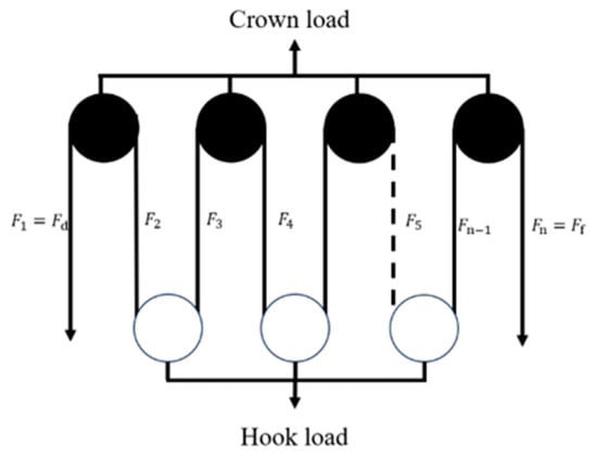
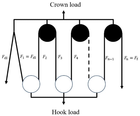
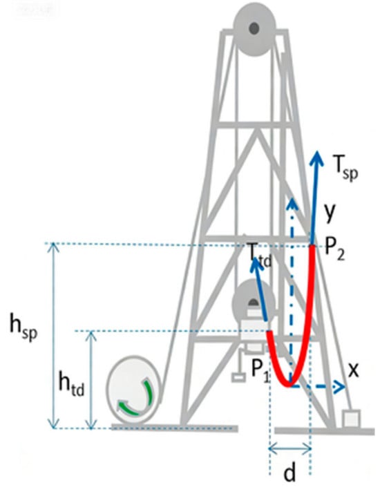
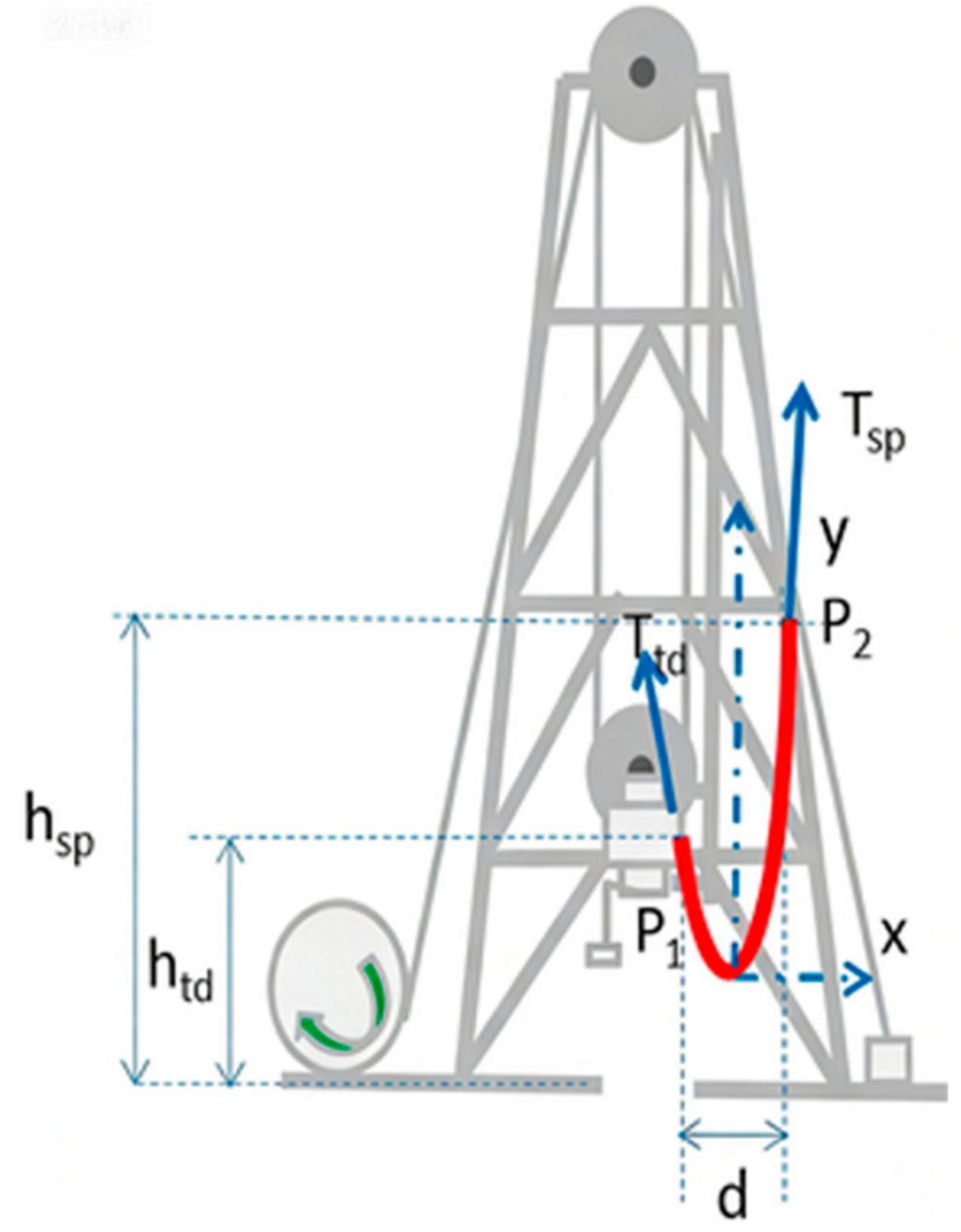
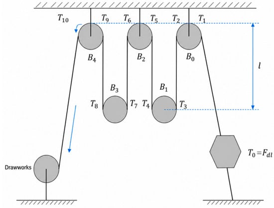
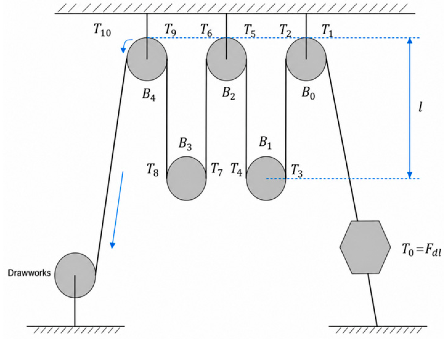
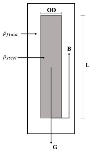
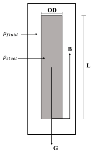
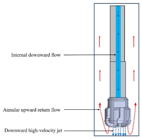
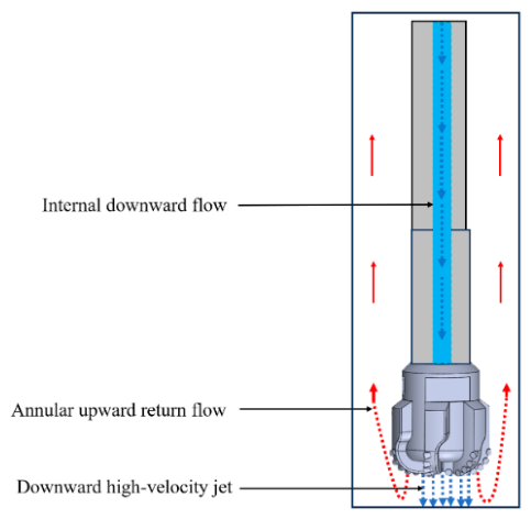
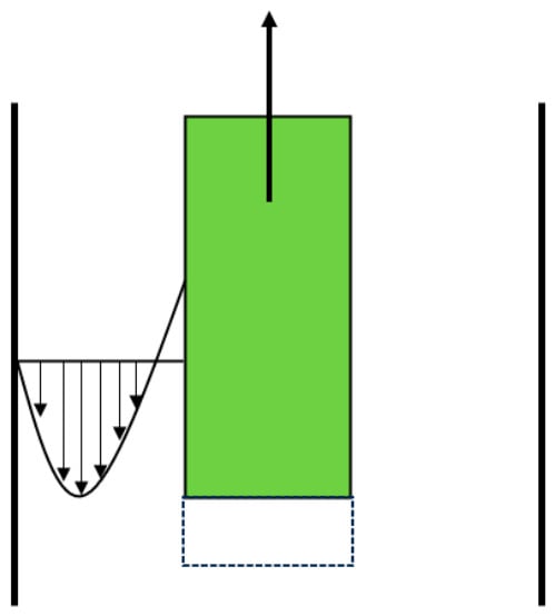
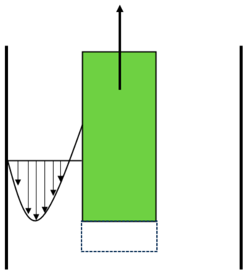
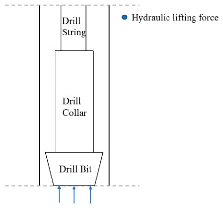
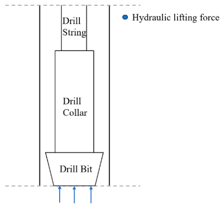
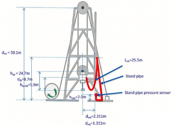
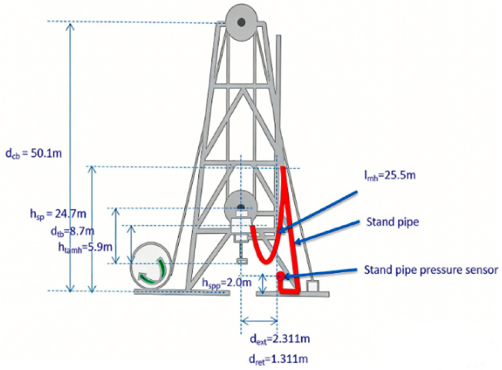
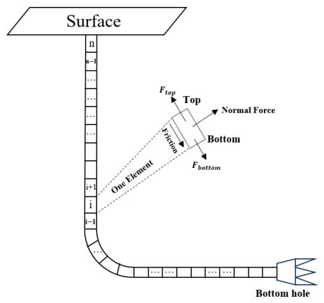
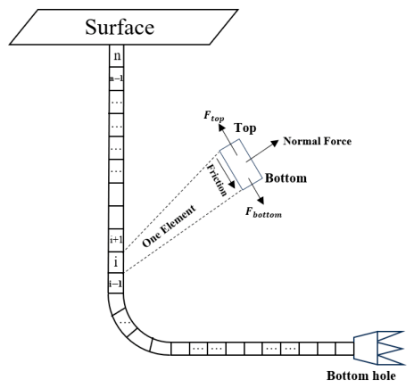
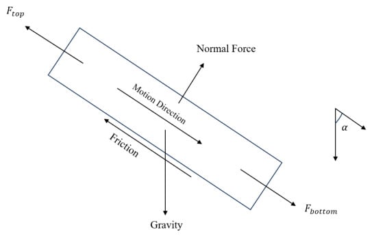
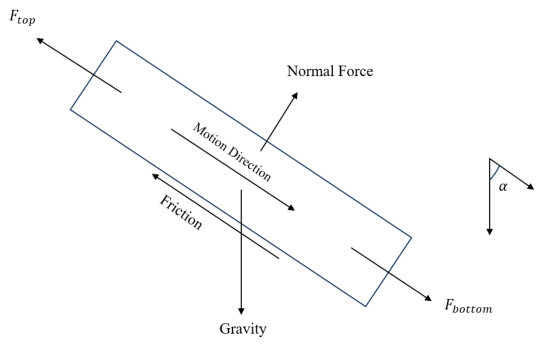
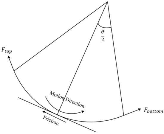
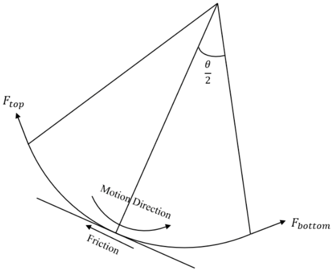
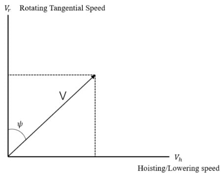
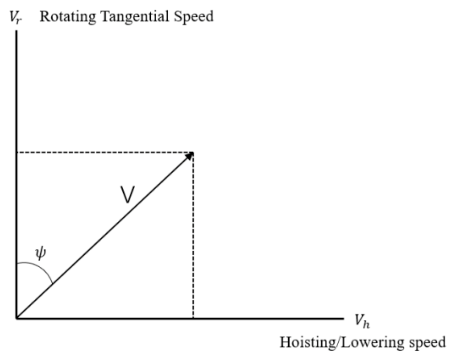
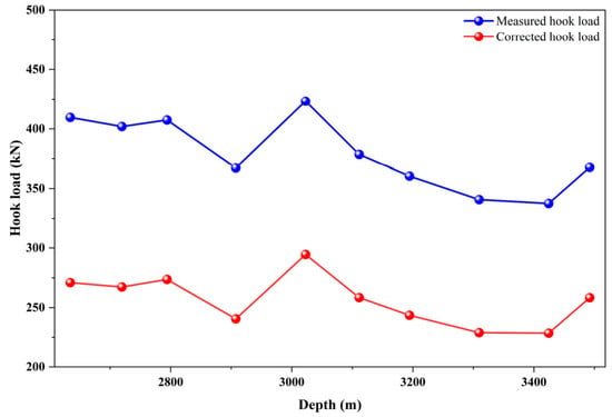
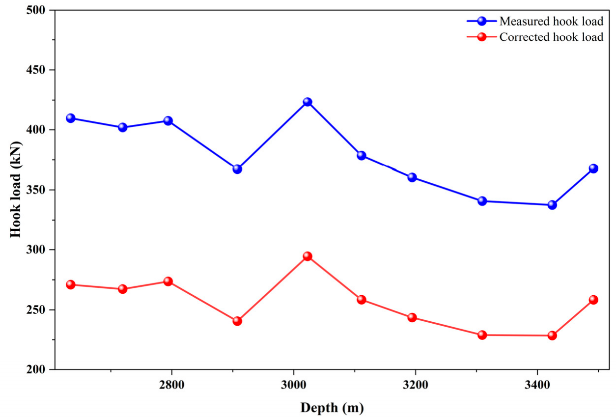
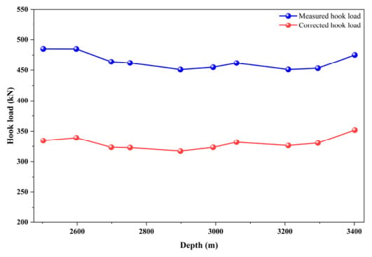
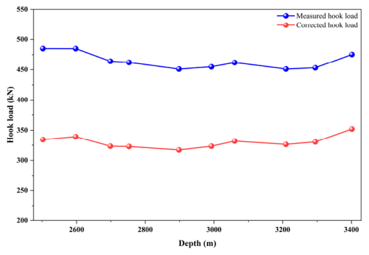

Disclaimer/Publisher’s Note: The statements, opinions and data contained in all publications are solely those of the individual author(s) and contributor(s) and not of MDPI and/or the editor(s). MDPI and/or the editor(s) disclaim responsibility for any injury to people or property resulting from any ideas, methods, instructions or products referred to in the content. |
© 2026 by the authors. Licensee MDPI, Basel, Switzerland. This article is an open access article distributed under the terms and conditions of the Creative Commons Attribution (CC BY) license.