A 3D Geometrical Model of Molecular Line Emission from Planetary Nebulae: Formulation and Applications

Abstract

Morpho-kinematic modeling of planetary nebulae (PNe) is important in reconstructing the three-dimensional structure and dynamics of PNe in an effort to understand their formation histories. Here, we present a flexible, modular method for 3D morpho-kinematic modeling of spatial–spectral mapping observations of PN molecular line emission. We show how a combination of basic geometric elements (an ellipsoid for the main nebula, an ellipsoidal mask for a lack of emission or cavity, and an elliptical ring for extended emission) can effectively reproduce the basic geometries and kinematics of the molecular emission regions of PNe, thereby providing constraints on key PNe parameters, including expansion velocity, physical size, and (hence) dynamical age. We apply PyPVNe to SMA and ALMA CO data cubes obtained for the PNe NGC 6720, NGC 3132, and Hubble 5. The results demonstrate the potential of our simple morpho-kinematic modeling methodology to investigate the origins and structural evolution of these and other molecule-rich PNe.

1. Introduction

Planetary nebulae (PNe) are the relatively brief ($\sim {10}^4–{10}^5$ yr) penultimate stage of stellar evolution of low- to intermediate-mass ($\sim 1–8{\mathrm{M}}_{\odot }$) stars [1,2]. While most PNe are dominated by ionized atomic gas, select PNe also contain cold (<100 K), dense ($\sim {10}^4–{10}^6{\mathrm{cm}}^{-3}$), massive envelopes of molecular gas and dust [3,4]. These molecular reservoirs within PNe—likely remnants of asymptotic giant branch (AGB) envelope material ejected shortly before PN formation—are readily detectable via millimeter-wave spectroscopy of rotational lines of CO and other relatively abundant molecular species [3,5]. Observations at high spatial and spectral resolution of multiple molecular species provide detailed insights into the density structure, kinematics, and chemical composition of these nebulae (e.g., [6,7,8]). High-resolution molecular line maps derived from such observations are essential for testing PN shaping models and probing how intermediate-mass stars enrich the interstellar medium (ISM) with nucleosynthesis products from their main-sequence and post-main-sequence (AGB) evolution [9]. Molecule-rich PNe are often ring-like or bipolar in morphology, with interacting binary evolution in systems with relatively massive progenitors considered the leading explanation for their origin ([4,7,8] and references therein), although the need for and role of binary companions in forming bipolar PNe remains debated [2]. Therefore, millimeter-wave CO data and modeling offer a powerful means to explore the shaping histories of these nebulae and their potential connections to binary evolution.

In this paper, we present a new approach to PNe 3D morpho-kinematic modeling, PyPVNe, which is designed for the interpretation of velocity-resolved emission-line mapping. PyPVNe has been specifically developed to model radio interferometric molecular line emission data such as those obtained with the Submillimeter Array (SMA) and the Atacama Large Millimeter/submillimeter Array (ALMA) but, in principle, can be applied across a range of wavelength regimes and position–velocity data collection techniques. Our modular, python-based approach, which was prototyped in two previous papers [6,7], involves building 3D geometrical representations of PN emission, comprised of combinations of simple structural elements (i.e., rings and ellipsoids) that can reproduce the emission features observed in position–velocity data. The resulting simple geometrical models can then be used to infer envelope ejection geometries and dynamical timescales. This straightforward modeling approach thereby yields insight into fundamental aspects of a PN’s formation and evolution, and hence its progenitor AGB star’s mass loss history. The basic structural and kinematic parameters thereby established can also serve as necessary inputs to more sophisticated morpho-kinematic modeling tools (e.g., SHAPEmol; [10]).

In Section 2, we describe the formulation of PyPVNe, and present a simple illustration of its use. The Python-based code, which remains under development, is available from the corresponding author upon reasonable request. In Section 3 and Section 4, we demonstrate the modeling framework’s capabilities via application to three well-studied, molecule-rich PNe (NGC 6720, NGC 3132, and Hubble 5), and we describe the resulting insights into the structures and kinematics of the molecular envelopes of these PNe. Concluding remarks are presented in Section 5.

2. Spatio-Kinematic Planetary Nebula Model: Formulation and Illustration

2.1. PNe Morpho-Kinematic Modeling

Morpho-kinematic modeling of PNe represents an essential means to understand their structures, shaping processes, evolution, emission properties, and their role in ISM chemical enrichment. One tool widely used for this purpose is SHAPE, an interactive 3D modeling environment particularly suited to the study of expanding nebulae such as PNe [11,12]. SHAPE combines the interactive design features of commercial 3D modeling software with astrophysical rendering tailored for nebular studies to effectively visualize whole nebulae. In practice, SHAPE gives users the ability to build and manipulate geometrical structures, representing nebular components (e.g., shells, rings, jets, or clumps) in a virtual three-dimensional environment. SHAPE was originally designed to model ionized gas within PNe and other nebulae; the recent extension SHAPEmol additionally includes molecular line radiative transfer, enabling spatio-kinematic modeling of the molecular gas components of PNe as well [10]. SHAPEmol hence represents the tool of choice for modeling detailed PN molecular gas structures, kinematics, and physical conditions (e.g., molecular column densities and optical depths).

In contrast, the PyPVNe modeling approach is specifically aimed at inferring the overall 3D structural and expansion geometries of PNe by approximating the morphological structures observed in molecular line emission data cubes obtained at high spatial and spectral resolution via interferometric mapping. This methodology provides a direct estimate of key parameters such as expansion velocities and dynamical ages, with the goal of obtaining a global, 3D view of the molecular morphology and kinematics of PNe. Unlike SHAPE and SHAPEmol, with their array of features and GUI-driven environments, PyPVNe is implemented entirely in Python (version 3.13.5 or later) and is fully reproducible and extensible within this open and widely accessible computational environment. Visualization is also supplemented using software such as GlueViz (version 1.12.0 or later) (https://glueviz.org/).

2.2. Modeling Approach and Components

PyPVNe modeling begins with a 3D FITS data cube obtained from observations of a PN as input, thereby ensuring the resultant model cube replicates the original file’s dimensional and data properties and hence facilitating straightforward model vs. data comparisons. In constructing the model, we iteratively adjust the geometric and kinematic input parameters and directly compare the resulting model cube with the observational cube within Python or 3D visualization tools such as GlueViz. The publicly available GlueViz software enables the user to overlay the data cube and resultant models directly on top of each other, with varying color and opacity to facilitate direct visual comparison of the spatial morphology, emission extent, and velocity structure between the model and observational data. Once a satisfactory agreement between the model and observations is achieved, Python is used to generate axial cross-sections for a more detailed comparison of the spatial and kinematic structure. Thus, this approach enables us to evaluate how effectively the model reproduces the observed emission structure and kinematics.

PyPVNe’s modular design allows the user to construct and combine a set of geometric components as needed to approximate observations. At present, the available components are an ellipsoid, an ellipsoidal mask, and an elliptical ring. Each of these components has corresponding modules (nebular ellipsoid, ellipsoidal mask and masked ellipsoid, and elliptical ring, respectively) which are designed to create models that reflect a specific feature within the PN data. The resultant nebular ellipsoid reflects emission from the main PN surface; the ellipsoidal mask removes emission from the surface of the nebular ellipsoid to reflect a lack of emission or cavity (as opposed to a physical structure); and the ellipsoidal ring approximates an extended, ring-like emission structure. Each of these modules is described in more detail in the Appendix. In the examples shown here (Section 2.3 and Section 3), we combine these components as needed to reproduce the observed emission distribution of a given PN. Additional structure modules will be provided in future versions of the code (see Section 5).

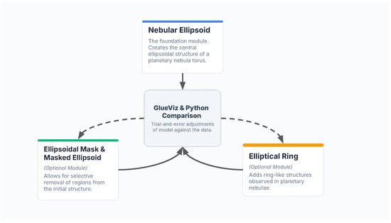
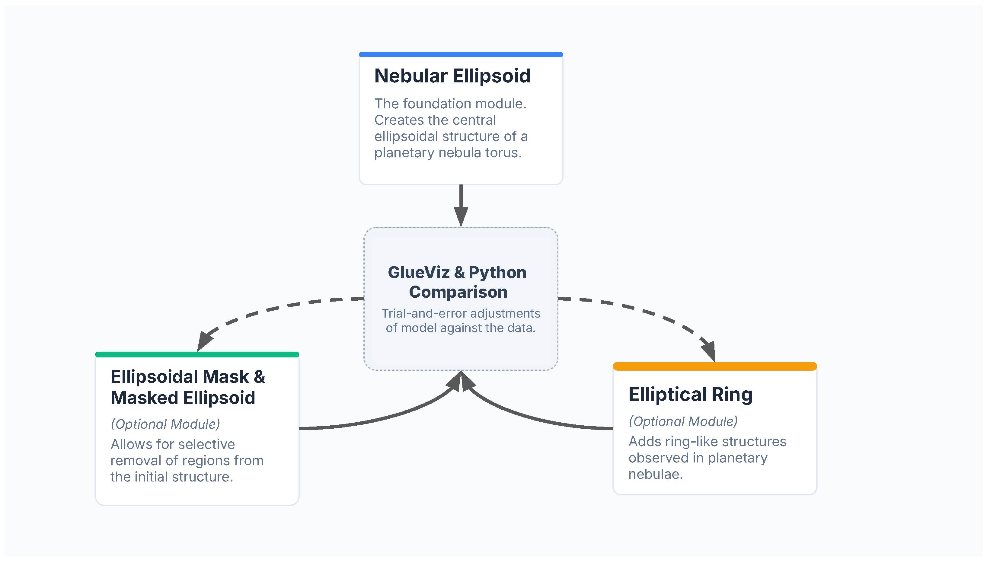
The overall PyPVNe workflow is illustrated in the form of a schematic flow chart in Figure 1. Although the specific choice of components depends on the desired nebular morphology, each model begins with the nebular ellipsoid module; this ellipsoid establishes the principal structure upon which additional components can be added. After each modeling step, the input parameters are iteratively adjusted through data-model comparisons in GlueViz and Python. In the various examples presented here, these comparisons are performed in the position–velocity domain, but it is also straightforward to compare (model vs. observed) spatially integrated emission line profiles (see, e.g., [6]).

Figure 1. Flowchart of the modular modeling workflow of PyPVNe. The nebular ellipsoid serves as the foundational structure, while optional modules such as the elliptical ring and ellipsoidal mask may also be used. After each modeling step, the input parameters are iteratively adjusted through data-model comparisons in GlueViz and Python.

2.3. Simple Example Model

To demonstrate how PyPVNe is used in practice, we describe a simple example of the construction of a planetary nebula model that comprises all three of the components. To set the model FITS file dimension and header information, this simple example model uses the NGC 6720 SMA data described in Section 3.2. However, this example serves to demonstrate the types of shapes and structures PyPVNe can generate and is not meant to reflect the structure of NGC 6720 or any other specific PN.

We list the input parameters used for the example model in Table 1; Table A2 contains a detailed description of each of these parameters. Summarizing, the example PN lies at a distance of 800 pc, has a dynamical age of 6000 yr; its main ellipsoidal structure has a major/minor axis ratio of 1:1/$\sqrt{2}$ and is expanding at 30 km s⁻¹ along its major axis. The example mask parameters (given by MaskParams), with coefficients $X,Y<1$ and $Z>1$ with the same (“pole-on”) orientation as the main ellipsoid (i.e., both orientations are set to $\left[000\right]$), generate the overall geometric structure of a truncated ellipsoid when combined with the main ellipsoid (whose parameters are given by Ellparams). Given these inputs, PyPVNe outputs the following nebular ellipsoid parameters: axial distances along $(X,Y,Z)$ of $8.70\times {10}^{17}$, $6.15\times {10}^{17}$, and $2.70\times {10}^{17}$ cm, and expansion velocities of 48.35, 34.19, and 14.99 ($\mathrm{km}{\mathrm{s}}^{-1}$), respectively. For the ellipsoidal mask, the half-axis dimensions are $4.35\times {10}^{12}$, $3.08\times {10}^{12}$, and $5.40\times {10}^{17}$ cm. The elliptical ring has semi-major and semi-minor axes of $1.16\times {10}^{18}$ cm and $8.73\times {10}^{17}$ cm, respectively, with a rotation of ${90}^{\circ }$ and inclinations of ${45}^{\circ }$ along both the x and y axes.

Table 1. Input parameter values used in the simple example model. Basic parameters of the PN to be modeled (distance, dynamical age, expansion velocity) are contained in PNparams; the main nebular ellipsoid and ellipsoidal mask parameters (relative axis lengths and orientations) are contained in Ellparams and MaskParams, respectively; and the dimensions, orientation, and expansion velocity of the elliptical ring are contained in the remaining (six) parameters. See corresponding Appendix A Table A2 for more details.

Input Parameter	Simple Example Model
PNparams	[800 pc, 6000 yr, 30.0 $\mathrm{km}{\mathrm{s}}^{-1}$]
Ellparams	[(1, ${\displaystyle \frac{1}{\sqrt{2}}}$, 1), [0 0 0]]
MaskParams	[(0.5, 0.5, 2), [0 0 0]]
x_axis_length	400 pixels
y_axis_length	300 pixels
z_rotation	90 degrees
x_inclination	45 degrees
y_inclination	45 degrees
ring_vexp	10 $\mathrm{km}{\mathrm{s}}^{-1}$

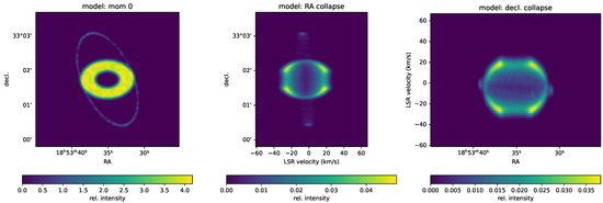
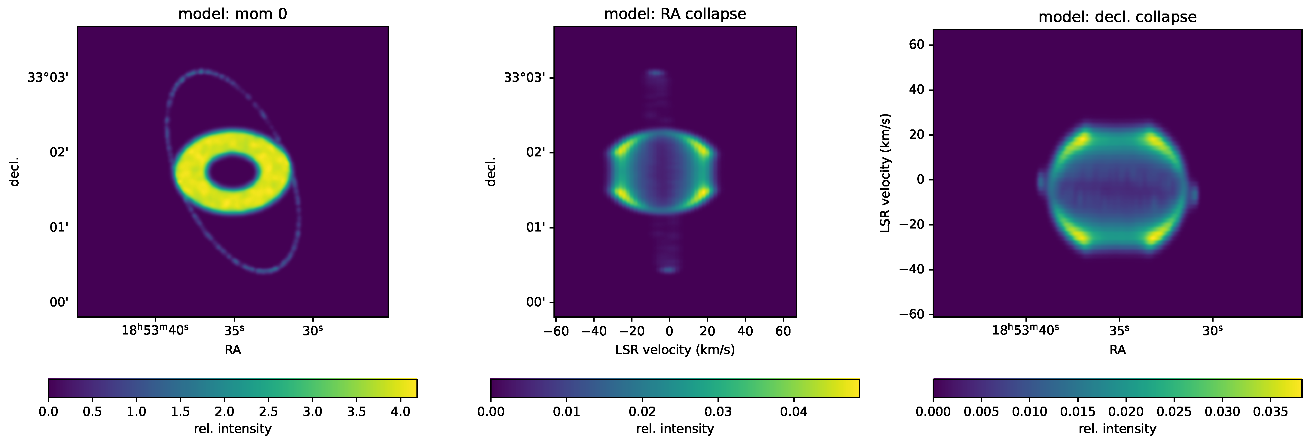
The resulting model projections are shown in Figure 2, in the form of velocity-integrated (“moment 0”) and position–velocity (P–V) images. Each of these images represents the model data cube as seen projected (“collapsed”) along a given axis. As both the main ellipsoid and mask are oriented with their major axes aligned along the line of sight, the masked (truncated) ellipsoidal shell appears in the moment 0 image as a ring with a central void. In contrast, in the P–V images, the masked shell is seen, in projection, as a truncated ellipse. The elliptical ring, which appears as such in the moment 0 image, is seen as a linear feature, with “ansae” at its ends, in the P–V images.

Figure 2. “Collapsed” views of the PyPVNe model data cube resulting from the input parameters listed in Table 1. The moment 0 (velocity-integrated) image is presented in the left panel, and position–velocity images resulting from integration along the RA and dec axes are presented in the center and right panels, respectively.

3. Spatio-Kinematic Modeling Examples: Targets and Observations

To further demonstrate potential applications of PyPVNe, we selected three planetary nebulae that are previously well-studied, rich in molecular gas, display a range of morphologies, have available high-resolution interferometric data, and would benefit from additional investigation and morpho-kinematic modeling: the Ring Nebula (NGC 6720), the Southern Ring Nebula (NGC 3132), and Hubble 5. These PNe also span a range of morphological and kinematic complexity: as we demonstrate below (Section 4), NGC 6720 represents a well-defined, truncated ellipsoid; NGC 3132 exhibits a more extended, elliptical shell with internal substructure and ring system; and Hubble 5 presents a highly asymmetric, central (equatorial) ellipsoid with superimposed, large ring structure. Together, these PNe illustrate the flexibility of PyPVNe in reproducing diverse nebular structures. In the cases of NGC 6720 and NGC 3132, comparison with previously published results using prototypes of PyPVNe provides points of reference, while for Hubble 5, the analysis below represents the first 3D spatio-kinematic modeling of its molecular emission region.

3.1. Target Nebulae

3.1.1. The Ring Nebula (NGC 6720)

The Ring Nebula (NGC 6720), an archetypal molecule-rich, “ring-like” PN, was imaged interferometrically in CO by Kastner et al. [7], who also reviewed the nebula’s structural and molecular-line observational history. Previous studies variably interpreted the nebula as either an ellipsoidal shell surrounded by a quasi-spherical halo [13,14] or as a bipolar structure with an equatorial waist and extended lobes viewed in projection [15,16]. More recently, Wesson et al. [17] proposed a twin-cone bipolar geometry viewed somewhat off-axis.

Using a prototype of the PyPVNe modeling framework to interpret SMA CO emission-line mapping of NGC 6720, Kastner et al. [7] modeled the PN’s molecular envelope as a truncated triaxial ellipsoid viewed nearly pole-on, with a dynamical age of ∼6000 yr and expansion velocity of ∼30 km s⁻¹, consistent with the model proposed by [13,14]. The CO emission is concentrated in a thin shell of clumps surrounding the ionized gas, and closely coincides with near-IR H₂ emission observed by JWST. Kastner et al. [7] concluded that the ellipsoidal molecular envelope was likely expelled in a brief, enhanced AGB star mass-loss episode about ∼6000 yr ago, and was subsequently truncated by binary-driven jets, consistent with the presence of a central dusty disk [18].

3.1.2. The Southern Ring Nebula (NGC 3132)

NGC 3132 is a nearby ($D=754$ pc), molecule-rich, ring-like PN that harbors a wide visual binary system [19]. Near-IR H₂ and millimeter-wave CO observations demonstrate the presence of a substantial molecular envelope [4,20,21]. Recent JWST imaging revealed a complex ring and arc system surrounding the central ionized region, possibly due to binary interactions, as well as a central dusty disk [22,23].

As for NGC 6720, Kastner et al. [6] used a prototype of PyPVNe to model their SMA CO mapping of NGC 3132. They found that the molecular envelope can be approximated as a twin-ring system, consisting of a bright, intrinsically elliptical equatorial torus viewed at low inclination, and a second, fainter ring oriented nearly orthogonally to the torus. The modeling indicated a dynamical age of ∼3700 yr, although with significant uncertainties due to the low inclination of the brighter equatorial structure.

3.1.3. Hubble 5 (Hb 5)

In sharp contrast to NGC 6720 and NGC 3132, Hubble 5 is a bipolar planetary nebula with a compact, bright central zone (≤4″) and extended lobes (∼60″ across the sky), with additional smaller central lobes [24,25,26,27]. It is an archetype of the class of high-excitation, molecule-rich bipolar PNe, with an intrinsic luminosity of ∼${10}^4$ $L_{\odot }$ and a central star effective temperature of ∼200 kK, consistent with a relatively massive progenitor star (see summary in [8]). Spectroscopic measurements reveal that the primary lobes exhibit high-velocity outflows of approximately 250 $\mathrm{km}{\mathrm{s}}^{-1}$ [24]. Morpho-kinematic modeling with SHAPE indicates the dynamical age of the nebula’s optical lobe system is ∼1500 yr for an adopted distance of 1.7 kpc [27]. Follow-up hydrodynamical simulations based on this model reproduced the observed morphology and expansion and suggested the likelihood of a progenitor mass exceeding 5 solar masses [28]. However, a more recent Gaia-calibrated distance scale puts the Hb 5 distance closer to 900 pc, suggesting an optical lobe dynamical age of just ∼800 yr [8].

Using both 12 m and Atacama Compact Array (ACA) ALMA observations, Moraga Baez et al. [8] detect ¹²CO emission tracing a 10″ north–south structure with fainter east–west “wings.” The strongest 12 m CO emission outlines a toroidal structure around the nebula’s narrow waist, with a projected expansion velocity of ∼30 km s⁻¹. In contrast, the extended wings show a slower expansion of ∼7 km s⁻¹. An additional, more diffuse, extended CO emission may trace the circular ring system seen in HST images. The ALMA–HST composite image presented in Moraga Baez et al. [8] (upper left panel of their Figure 3) demonstrates how the brightest CO emission appears to trace a nearly edge-on torus encircling the nebula’s waist, with the southern-most portion of this CO structure overlapping with a small optical emission lobe. The fainter, extended CO “wings” detected in the 12 m maps are likely associated with the front wall of the eastern optical lobe and the back wall of the western lobe. From a simple 2D expanding torus model of the CO emission as mapped by ALMA, and adopting $D=900$ pc, Moraga Baez et al. [8] infer a molecular torus expansion velocity of $30 \mathrm{km}{\mathrm{s}}^{-1}$ and a torus dynamical age of 500 yr.

3.2. Observations: Interferometric Millimeter-Wave CO Mapping

Here, we reanalyze velocity-resolved interferometric CO mapping observations of ¹²CO ($J=2\to 1)$ ($\nu =230.538$ GHz, $\lambda \sim 1.3$ mm) obtained with the SMA for NGC 6720 and NGC 3132 and with ALMA for Hubble 5. The SMA provided the necessary field of view and sensitivity to the extended emission of the two northern hemisphere nebulae, NGC 6720 and NGC 3132, while Hb 5 was observed as part of the ALMA bipolar planetary nebulae molecular line survey presented in Moraga Baez et al. [8]. The respective SMA and ALMA array configurations and observations, summarized in Table 2, are described in detail in Kastner et al. [7], Kastner et al. [6], and Moraga Baez et al. [8].

Table 2. Summary of ¹²CO ($J=2\to 1$) observations of the three target planetary nebulae. Listed are the mm wave interferometric facility used, synthesized beam size, and velocity resolution. Data adapted from [6,7] (NGC 3132 and NGC 6720, respectively), and [8] (Hb 5).

Object	Array	Beam Size	Velocity Resolution
NGC 6720	SMA	$3.3^{″}\times 2.9^{″}$	2 km s−1
NGC 3132	SMA	$6.{47}^{″}\times 2.5^{″}$	2 km s−1
Hubble 5	ALMA	$1.6^{″}\times 1.{16}^{″}$	0.734 km s−1

4. Spatio-Kinematic Modeling Examples: Results

The following examples of PyPVNe modeling of the interferometric CO observations of NGC 6720, NGC 3132, and Hb 5 illustrate how application of this modeling framework can reveal the complex intrinsic molecular gas structures of these PNe, thereby illuminating fundamental aspects of their morphologies and evolution. In particular, upon finding reasonable agreement between the model and data, we obtain estimates of the dynamical age and 3D structure and kinematics of each planetary nebula. More specifically, given a PN’s distance and assumed age (as well as an initial rough estimate of the PN expansion velocity), an accurate nebular ellipsoid model resulting from our present trial-and-error methodology yields estimates of the ellipsoid axial aspect ratios and physical (linear) dimensions, as well as the expansion velocity along, and rotation angle with respect to, each axis. For an accurate ellipsoidal mask model (if applicable), we obtain estimates of the axial dimensions and rotation angles of the cavity. For an accurate elliptical ring model (if applicable), we obtain the ring’s semi-major and semi-minor axes and the rotation and inclination angles of the ring, given an assumed ring expansion velocity.

Note that “reasonable agreement” is determined through visual inspection of overlays between the model and observational data cubes rather than through a formal statistical fit. Agreement is assessed based on the correspondence between the observed and modeled spatial morphology, projected axial dimensions, axial cross-sections, and kinematic behavior as observed in Python or GlueViz visualizations. As such, the dimensions of the ellipsoid surface and hence derived quantities are uncertain, typically at the ∼10% level.

Furthermore, in the absence of proper motion measurements (via, e.g., multi-epoch subarcsecond imaging) that can constrain a PN’s transverse expansion speeds, morpho-kinematic modeling inevitably leads to degeneracies between inferred PN dynamical age, dimensions, and expansion velocity. The onset of nebular photoionization by the central post-AGB star, which would likely accelerate the expansion of the molecular envelope—leading to an underestimate in the elapsed time since onset of envelope ejection—potentially represents an additional complication in the inference of dynamical ages [7].

With those caveats in mind, the following details results obtained from morpho-kinematic modeling of the interferometric mapping of CO emission from NGC 6720, NGC 3132, and Hubble 5. Input and output PyPVNe model parameters for each of these three cases are listed in Table 3 and Table 4, respectively.

Table 3. Input parameter values for the NGC 6720, NGC 3132, and Hubble 5 models, adopted from Kastner et al. [6,7], Moraga Baez et al. [8]. The first three input parameters are used in the creation of the nebular ellipsoid and mask; the latter six are utilized in the ring module.

Input Parameter	NGC 6720	NGC 3132	Hubble 5
PNparams	[782 pc, 6000 yr, 30.0 $\mathrm{km}{\mathrm{s}}^{-1}$]	[754 pc, 6000 yr, 25.0 $\mathrm{km}{\mathrm{s}}^{-1}$]	[900 pc, 500 yr, 50.0 $\mathrm{km}{\mathrm{s}}^{-1}$]
Ellparams	[(1,${\displaystyle \frac{1}{\sqrt{2}}}$,${\displaystyle \frac{1}{\sqrt{1.5}}}$), [−1° 0° −20°]]	[(${\displaystyle \frac{1}{\sqrt{1.75}}}$, 1, ${\displaystyle \frac{1}{\sqrt{4}}}$), [0° −5° −30°]]	[(${\displaystyle \frac{1}{\sqrt{22}}}$, ${\displaystyle \frac{1}{\sqrt{4}}}$, 1), [−10° 2° −45°]]
MaskParams	[(0.6, 0.8, 2.0), [12° −5° −20°]]	[(0.99, 0.99, 2), [0° 0° −30°]]	None
x_axis_dia	None	75 pixels	190 pixels
y_axis_dia	None	90 pixels	190 pixels
z_rotation	None	−30°	0°
x_inclination	None	20°	0°
y_inclination	None	−55°	0°
ring_vexp	None	25 $\mathrm{km}{\mathrm{s}}^{-1}$	10 $\mathrm{km}{\mathrm{s}}^{-1}$

Table 4. Output parameter values from NGC 6720, NGC 3132, and Hubble 5 models. Semi-axis lengths given in cm and velocities given in $\mathrm{km}{\mathrm{s}}^{-1}$ corresponding to each of the ellipsoidal axes ($X,Y,Z$). No cavity (ring) axial distances are listed for Hubble 5 (NGC 6720) since PyPVNe did not utilize the ellipsoidal cavity (elliptical ring) module.

Output Parameter	NGC 6720	NGC 3132	Hubble 5
PN semi-axis lengths (cm)	($5.4\times {10}^{17},3.8\times {10}^{17}$, $4.4\times {10}^{17}$)	($2.1\times {10}^{17},2.8\times {10}^{17}$, $1.4\times {10}^{17}$)	($1.6\times {10}^{16},3.8\times {10}^{16}$, $7.5\times {10}^{16}$)
PN axial expansion velocities ($\mathrm{km}{\mathrm{s}}^{-1}$)	(30.0, 21.2, 24.5)	(11.8, 15.8, 10.2)	(10.7, 25.0, 50.0)
Cavity semi-axis lengths (cm)	($2.3\times {10}^{17},3.1\times {10}^{17}$, $8.8\times {10}^{17})$	($2.1\times {10}^{17},2.8\times {10}^{17}$, $3.7\times {10}^{17}$)	None
Ring semi-major/semi-minor axes (cm)	None	($2.5\times {10}^{17}$, $2.1\times {10}^{17}$)	($2.7\times {10}^{17}$, $2.7\times {10}^{17}$)

4.1. Ring Nebula (NGC 6720) Model

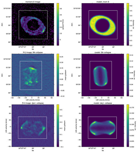
Our NGC 6720 SMA CO data and corresponding PyPVNe model are presented in Figure 3. In creating this model, we made use of the nebular ellipsoid and masking modules (no ring). The essential planetary nebula parameters PNparams we adopted (see Table 3) are a distance D of 782 pc, a dynamical age of 6000 yr, and an initial estimated expansion velocity V of 30.0 $\mathrm{km}{\mathrm{s}}^{-1}$. Per Figure 3 and [7], the model ellipsoid we obtain from the PyPVNe modeling is significantly nonspherical, with relative X:Y:Z axis ratios of about 1:$0.71$:$0.82$, viewed nearly pole-on (along the Z axis) and rotated through a position angle of ∼70°. Further, this nebular ellipsoid is truncated by a more elongated, more inclined ellipsoid (see corresponding Table 3 MaskParams), forming a nearly circular cross-section near the center of the nebula, accounting for the apparent absence of emission at velocities of ∼$\pm 20$ km s⁻¹, with respect to the systematic (see Figure 3), or at a distance of ∼$4\times {10}^{17}$ cm along the Z axis. The dimensions of this ellipsoidal mask are not tightly constrained, but we find that a mask with dimensions given in Table 4 inclined by 12° and −5° with respect to the other axes at a position angle of 160° (E from N), produces a truncated ellipsoid model whose overall morphology agrees with that seen in the SMA ¹²CO(2–1) data.

Figure 3. NGC 6720 SMA data and model moment 0 and position–velocity images of ¹²CO(2–1) emission. The white square in each panel has dimensions of 80 × 80 kau², assuming the Gaia parallax distance to NGC 6720 (782 pc) and the CO envelope’s extent along the z-axis from the masked ellipsoid model. The P–V image obtained from a RA (declination) collapse corresponds to a N–S (E–W) slit.

The model presented here is very similar to that in [7], using the same coding process, but with refined input parameters. Specifically, the prior model had an ellipsoidal mask of semi-minor axis of $2.3\times {10}^{17}$ cm and a major axis of $1.8\times {10}^{18}$ cm, inclined by ${12}^{\circ }$ at a position angle of 160° (measured E from N) with respect to the line of sight; in this paper, we additionally introduce an inclination of $5^{\circ }$ away from the declination axis. This changed the lower extent of the molecular torus in the declination collapse frame (to reflect the edge of emission) and the intensities of the moment 0 (the near uniformity) and RA collapse frames (upper right bright region), thereby more accurately reflecting the data. However, generally speaking, the same conclusions and inferences hold for this model as those presented in [7].

4.2. Southern Ring Nebula (NGC 3132) Model

Our NGC 3132 SMA CO data and corresponding PyPVNe model are presented in Figure 4. In creating this model, we made use of the nebular ellipsoid, masking, and ring modules. The essential planetary nebula parameters PNparams we adopted (Table 3) are a distance D of 754 pc, a dynamical age of 3700 yr, and an initial estimated expansion velocity V of 25 $\mathrm{km}{\mathrm{s}}^{-1}$. Per Figure 4, the model ellipsoid has relative $X:Y:Z$ axis ratios of about $0.76:1.00:0.5$, viewed within ∼5° of pole-on (along the Z axis) and rotated through a position angle of ∼60°. Further, this nebular ellipsoid is truncated by a slightly smaller, slightly less inclined ellipsoid (see corresponding Table 3), to produce the relatively thin, ring-like morphology we observe.

Figure 4. NGC 3132 SMA data and model moment 0 and position–velocity images of ¹²CO(2–1) emission. The P-V image: RA collapse frame (P-V image: Dec collapse frame) is equivalent to a N-S slit (E-W slit).

In addition to the truncated nebular ellipsoid, we also observe a much fainter, differently inclined ring. This ring is estimated to have an expansion velocity of ∼25 $\mathrm{km}{\mathrm{s}}^{-1}$ and semi-major and semi-minor axes of dimensions comparable to those of the nebular ellipsoid (see Table 4), such that the two structures intersect. However, the superimposed ring is rotated through a larger position angle and has been inclined 45° away from the declination axis (clockwise) and 20° towards the RA axis, as seen in Figure 4 mom0 frame.

In contrast to the NGC 3132 model presented in Kastner et al. [6], which utilized a dual-ring modeling structure, the model presented here consists of a highly truncated/masked ellipsoid with a ring. This model represents an improvement from the previous approach in that it does not require artificial extension along the line of sight through velocity smearing, as was imposed in the two-ring model. Further, the model presented in [6] restricted the ring rotations to orthogonal directions, whereas here we employ free rotation parameters. Despite the inherent structural differences between the models presented here and in [6], both effectively reproduce the overall morphology of the nebula. Our truncated/masked ellipsoid model also supports the PN dynamical age of 3700 yr obtained from model A in [6].

4.3. Hubble 5 Model

Unlike NGC 6720 and NGC 3132, whose SMA ¹²CO(2-1) observations were previously modeled using similar methodology [6,7], our modeling of the ALMA observations of Hb 5 [8] provides a new interpretation of the molecular gas structure in this PN. Distance estimates for Hb 5 span a wide range, reflecting uncertainties associated with its complex bipolar morphology and differing distance methods [27,29,30,31,32]. Following Moraga Baez et al. [8], we adopt a distance of 900 pc and a corresponding molecular envelope dynamical age of 500 yr for our model inputs (Table 3).

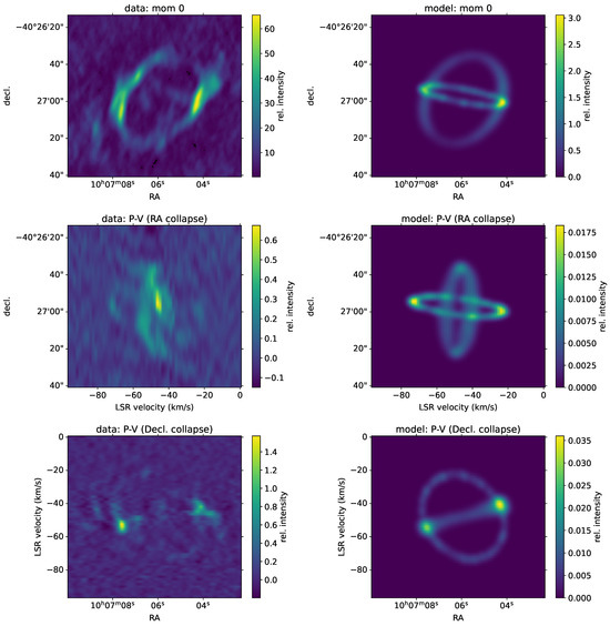
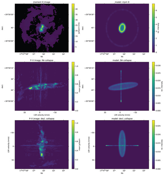
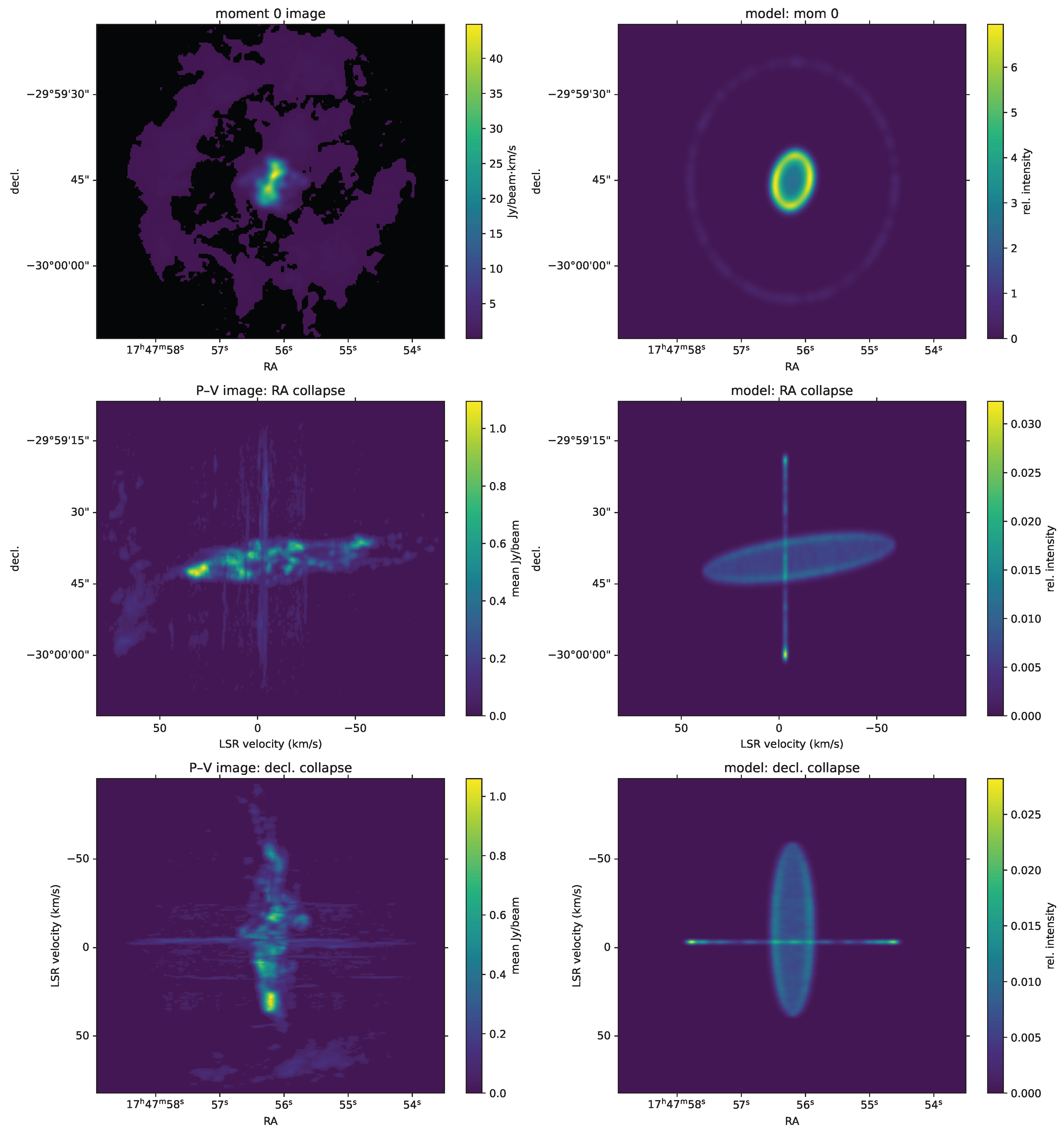
The ALMA CO observations and corresponding PyPVNe model, illustrated in Figure 5, reveal a bright, elongated N–S molecular structure concentrated around the nebular waist, with fainter E–W extended emission. As noted by Moraga Baez et al. [8], the brightest CO emission traces an elliptical torus with a projected expansion velocity of ∼30 $\mathrm{km}{\mathrm{s}}^{-1}$, while the more extended component exhibits lower velocities of ∼10 $\mathrm{km}{\mathrm{s}}^{-1}$. Additional faint emission may correspond to concentric structures previously identified in HST imaging, which we have modeled here as a ring.

Figure 5. Hubble 5 ALMA data and model moment 0 and position–velocity images of ¹²CO(2–1) emission. The P-V image: RA collapse frame (P-V image: Dec collapse frame) is equivalent to an N-S slit (E-W slit).

On the other hand, HST optical forbidden-line images show prominent E–W bipolar lobes that are morphologically distinct from the CO emission, indicating that the ionized and molecular components trace different physical phases of the nebula. The optical lobes likely arise from high-velocity ionized outflows, whereas the CO traces a denser, slower molecular envelope. These differences suggest either distinct ejection episodes or strong post-AGB shaping of multiple mass-loss phases.

The CO data are modeled using a combination of a highly elongated nebular ellipsoid and a low-velocity ring component. Corresponding inputs and outputs are presented in Table 3 and Table 4. The ellipsoid has relative X:Y:Z axis ratios of approximately $0.21$:$0.5$:1, is viewed within ∼10° of pole-on, and rotated through a position angle of ∼45°. The model also exhibits a strongly anisotropic velocity field with a factor of ∼5 contrast between minimum and maximum expansion velocities, with the fastest expansion reaching (∼50 km s⁻¹) oriented nearly along the line of sight.

Faint CO emission surrounding the core is confined to narrow velocity channels and is tentatively associated with optical ring structures seen in HST images. The narrow velocity structure is likely indicative of optical depth effects—specifically, limb brightening within a system comprised of a set of nested spheres, or the bright rims of a 3D spiral system. Although this component does not form a clearly defined ring in integrated intensity maps, its velocity coherence and spatial correspondence motivate its representation using the ring module. A low-surface-brightness ellipsoidal shell could also reproduce aspects of this emission, but given the limited signal-to-noise and fragmented morphology, the current data do not uniquely distinguish between these geometries. Thus, this component is modeled as a nearly circular ring lying within the RA-Dec plane, with an assumed expansion velocity of ∼10 $\mathrm{km}{\mathrm{s}}^{-1}$.

Together, the ionized bipolar lobes and molecular torus highlight the multi-phase structure of Hb 5. The bipolar lobes trace fast (∼250 $\mathrm{km}{\mathrm{s}}^{-1}$) ionized outflows consistent with interacting-winds shaping of energetic outflows, while the molecular torus represents slower AGB-derived material that likely predates and helps collimate the ionized outflows. The observed asymmetries, clumpiness, and equatorial density are consistent with shaping by binary interactions, which induce equatorial compression and collimated outflows [24]. The larger-scale ring structures seen in HST imaging and in CO may be indicative of earlier stages of binary interactions, preceding the onset of equatorial and polar outflows.

5. Concluding Remarks

The foregoing examples demonstrate the physical insights that can be gained concerning the large-scale structure and dynamics of molecular gas in PNe via application of the PyPVNe modeling framework now under development. The resulting 3D morpho-kinematic models of PNe molecular line emission are directly analogous to, and complement, models of the 3D geometry and kinematics of ionized gas as obtained from HST imaging and ground-based spectroscopy (e.g., [33,34]). Modeling of interferometric maps of PNe molecular emission similarly illuminates AGB mass-loss geometry, binary-driven wind interactions, and the fate of dense, neutral circumstellar gas in the final stages of the evolution of intermediate-mass stars.

Rather than performing detailed non-LTE radiative transfer calculations or self-consistent molecular excitation modeling, PyPVNe is designed to provide a flexible and computationally efficient framework for approximating the large-scale geometry and kinematics of molecular gas structures in PNe. In this sense, PyPVNe is complementary to more advanced modeling tools, as it is primarily intended for initial, exploratory structural interpretation of interferometric molecular-line datasets, yet is also intended to be easily extensible. Near-term improvements to be made will likely include refinements of existing structure modules and/or inclusion of additional modules, so as to accommodate geometric elements such as finite-thickness shells, polar lobes/cones, and linear features (jets); enabling automation of both initial parameter estimation and iterative model fitting; providing additional tools for data and model visualizations and comparisons (e.g., extraction of P–V images at arbitrary position angles); and allowing nebular component offsets (centering) and specification of “standard” structure orientation angles (position angle and inclination) as input parameters.

Moving forward, the continued development of PyPVNe, and its application to new interferometric datasets and various chemical tracers, will support a more holistic understanding of the origin and evolution of molecular gas within PNe. For example, by modeling the spatial and kinematic distributions of CO, HCO⁺ and CO⁺ in the same PN (e.g., NGC 7027 [35]), we can reveal how different envelope regions respond to UV and X-ray irradiation, distinguishing between photo-dissociation regions (PDRs) and X-ray dominated regions (XDRs) [36].

Such PN molecular line emission modeling also connects directly with growing efforts in PN astrochemistry. Various studies (e.g., [8,37,38,39] and references therein) have shown how molecules like CN, HCN, and SiO are relatively abundant in evolved PNe, and how their abundances relate to stellar radiation and envelope structure. Including these species in morpho-kinematic emission-line modeling will offer a spatially resolved, 3D view of PNe envelope chemistry and excitation conditions.

Appendix A.1. Nebular Ellipsoid Module

We designed the nebular ellipsoid module to generate an FITS file containing a nebular ellipsoid, i.e., an ellipsoidal shell defined by three principal axes (major, minor, and line-of-sight) that describe the overall size, orientation, and aspect ratios of the observed planetary nebula. The nebular ellipsoid is defined using the equation

$${\displaystyle \frac{x^2}{a^2}}+{\displaystyle \frac{y^2}{b^2}}+{\displaystyle \frac{z^2}{c^2}}=1,$$

(A1)

where a, b, and c are the semi-axis lengths of the nebular ellipsoid. We parameterize the axis lengths in terms of dimensionless scaling coefficients A, B, and C, such that

$$a={\displaystyle \frac{1}{\sqrt{A}}},b={\displaystyle \frac{1}{\sqrt{B}}},c={\displaystyle \frac{1}{\sqrt{C}}}.$$

(A2)

This parameterization ensures positive-definite axis lengths and naturally encodes the relative axis ratios of the ellipsoid. Substituting these definitions into the ellipsoid equation yields an equivalent quadratic form:

$$A{x}^2+B{y}^2+C{z}^2=1.$$

(A3)

Table A1 provides the function call, necessary function inputs, and any outputs. The function inputs include the following: directory, filename, PNparams, Ellparams, savedir, and savename. directory and filename define the filepath and name of the observational data file, used for retrieving the data file shape and necessary header parameters. Table A2 summarizes the contents for each of the primary input parameters.

Table A1. Table of function calls, necessary inputs, and any outputs for model formulation models. The directory and filename inputs for create_ellipsoid() and create_ellipsoid_mask() are the filepath and name of the PN observational data cube. The filenames input for masked_ellipsoid() are the names (and corresponding paths) of the resultant files from the prior two function calls. The directory and filename inputs for create_elliptical_ring() are the path and name of the negative masked ellipsoid file from masked_ellipsoid() if applicable, or the path and name of the nebular ellipsoid file. The intensity_scaling input sets the relative intensity of the ring. The savedir and savename(s) input for all of the function calls sets the directory and filename(s) of the files to be created by that module. The contents of the other main inputs are described in Table A2. The ellipseparams output is a tuple of arrays of physical axial distances (km), velocities (in $\mathrm{km}{\mathrm{s}}^{-1}$), and angles (radians) of the nebular ellipsoid. The maskparams output is a tuple of arrays listing the mask center, mask physical axial distances (km), and mask rotation angles (radians).

Function Call	Inputs	Outputs
create_ellipsoid()	directory, filename, PNparams, Ellparams, savedir, savename	None
create_ellipsoid_mask()	directory, filename, PNparams, Ellparams, Maskparams, savedir, savenames	ellipseparams, maskparams
masked_ellipsoid()	filenames, savedir, savename	None
create_elliptical_ring()	directory, filename, PNparams, savedir, savename, x_axis_length, y_axis_length, intensity_scaling, vexp, optional: z_rotation, x_inclination, y_inclination	ring_phys_lengths, ring_rotation

Table A1. Table of function calls, necessary inputs, and any outputs for model formulation models. The directory and filename inputs for create_ellipsoid() and create_ellipsoid_mask() are the filepath and name of the PN observational data cube. The filenames input for masked_ellipsoid() are the names (and corresponding paths) of the resultant files from the prior two function calls. The directory and filename inputs for create_elliptical_ring() are the path and name of the negative masked ellipsoid file from masked_ellipsoid() if applicable, or the path and name of the nebular ellipsoid file. The intensity_scaling input sets the relative intensity of the ring. The savedir and savename(s) input for all of the function calls sets the directory and filename(s) of the files to be created by that module. The contents of the other main inputs are described in Table A2. The ellipseparams output is a tuple of arrays of physical axial distances (km), velocities (in $\mathrm{km}{\mathrm{s}}^{-1}$), and angles (radians) of the nebular ellipsoid. The maskparams output is a tuple of arrays listing the mask center, mask physical axial distances (km), and mask rotation angles (radians).

Function Call	Inputs	Outputs
create_ellipsoid()	directory, filename, PNparams, Ellparams, savedir, savename	None
create_ellipsoid_mask()	directory, filename, PNparams, Ellparams, Maskparams, savedir, savenames	ellipseparams, maskparams
masked_ellipsoid()	filenames, savedir, savename	None
create_elliptical_ring()	directory, filename, PNparams, savedir, savename, x_axis_length, y_axis_length, intensity_scaling, vexp, optional: z_rotation, x_inclination, y_inclination	ring_phys_lengths, ring_rotation

Table A2. Table of key input parameters and their contents for model modules. The PNparams input is a list of key PN properties based on literature values.

Input Parameter	Contents
PNparams	list of distance (km), age (s), and expansion velocity ($\mathrm{km}{\mathrm{s}}^{-1}$)
Ellparams	array of three (unitless) scaling coefficients and an array of rotation angles (degrees) for each of the axes
Maskparams	tuple of (unitless) axis scalings (relative to nebular ellipsoid axis lengths) and an array of rotation angles (degrees) for each of the axes
x_axis_length and y_axis_length	(pixel) lengths along the ring’s x- and y-axes, respectively
$\mathbf{optional}$: z_rotation, x_inclination, and y_inclination	angles (degrees) to rotate the ring in the x-y plane (clockwise) and incline it toward the x/y-axis, respectively

Table A2. Table of key input parameters and their contents for model modules. The PNparams input is a list of key PN properties based on literature values.

Input Parameter	Contents
PNparams	list of distance (km), age (s), and expansion velocity ($\mathrm{km}{\mathrm{s}}^{-1}$)
Ellparams	array of three (unitless) scaling coefficients and an array of rotation angles (degrees) for each of the axes
Maskparams	tuple of (unitless) axis scalings (relative to nebular ellipsoid axis lengths) and an array of rotation angles (degrees) for each of the axes
x_axis_length and y_axis_length	(pixel) lengths along the ring’s x- and y-axes, respectively
$\mathbf{optional}$: z_rotation, x_inclination, and y_inclination	angles (degrees) to rotate the ring in the x-y plane (clockwise) and incline it toward the x/y-axis, respectively

PNparams is a list of key PN properties adopted from the literature, including distance (km), age (s), and expansion velocity ($\mathrm{km}{\mathrm{s}}^{-1}$). Ellparams is a list containing two arrays specifying relative axis scalings (a:b:c) and the rotation angles of the ellipsoid relative to the three principal axes of the data cube. The axis scalings are dimensionless quantities defining the relative proportions of the ellipsoid. The orientation vector specifies successive rotational tilt angles, in (x, y, z) order, with respect to the data-cube axes, with both positive and negative rotation angles permitted. Although 3D orientations are commonly expressed using direction cosines, the present model parametrizes orientation through rotation angles relative to the data-cube axes. The equivalent direction cosines can be obtained from the rotated unit vector of the ellipsoid’s principal axis.

Finally, savedir and savename define the directory the model file will be saved in (can be the same as the input directory or different) and under what name. Overall, the create_ellipsoid function uses these input parameters to generate a FITS file containing a nebular ellipsoid that approximates the primary structure of the target PN.

The resulting model ellipsoid can then be directly compared with the observational data cube in GlueViz or Python in order to refine the input parameters. While the data and model intensity scales may differ in the visualization due to the arbitrary (non-physical) emission intensity assignment of the code, this difference is inconsequential, given that the goal is to approximate the overall nebular shape and kinematic structure. Further, this module can be optionally modified to calculate and output desired information about the model ellipsoid, such as the physical lengths of the three axes or the rotation angles.

Appendix A.2. Ellipsoidal Mask and Masked Ellipsoid Modules

We designed the ellipsoidal mask module to generate a FITS file containing an ellipsoidal mask that approximates a cavity or void within the main structure of a PN. This lack of central emission is possibly a result of gas clearing, molecule disassociation, or chemical processing by the evolving central star and its outflows, leaving the remaining molecular gas to be concentrated in a surrounding shell or toroidal structure, further out from the central star system. Table A1 provides the function call, necessary inputs, and any outputs of this module. This module shares the directory, filename, PNparams, Ellparams, and savedir inputs used in the nebular ellipsoid module. Table A2 describes the contents of Maskparams: a list containing a tuple of axis scalings, and an array of rotation angles (degrees) for each of the three mask axes. The scaling coefficients are defined relative to the dimensions of the nebular ellipsoid, and hence they appear as decimals rather than fractions (as used for the nebular ellipsoid scalings). However, the orientation vector of the mask acts similarly to that of the nebular ellipsoid; both orientation vectors are defined with respect to the data cube axes, since we have observed that the ring can be very differently orientated from the nebular ellipsoid.

savenames specifies two filenames within a tuple, containing positive and negative versions of the model mask; the former is purely for visualization purposes, while the latter is for model application.

The module outputs then reiterates some input parameters and provides the axial distances (km) of both the nebular ellipsoid and ellipsoidal mask, along with the expansion velocity along each of the three axes. In general, the create_ellipsoid_mask function uses these parameter inputs to generate FITS files of positive and negative images of an ellipsoidal mask, and output relevant nebular ellipsoid and mask parameters.

The masked ellipsoid module (whose function call and inputs can be seen in Table A1) then takes the files created by the nebular ellipsoid and ellipsoidal mask modules and effectively combines them to form a new file named savename containing a masked ellipsoid, saved within savedir.

Appendix A.3. Elliptical Ring Module

The elliptical ring module generates an FITS file containing an elliptical ring that approximates the ring-like structures frequently seen superimposed on and/or surrounding the central region of a PN. Table A1 provides the function call, necessary function inputs, and any outputs of this module. This module again shares the PNparams with the previous modules. The directory and filename parameters in this module now specify the path and filename of the masked ellipsoid (rather than the observational data), and the savedir and savename are updated for the module’s resultant directory and filename.

Table A2 describes the contents for each of the elliptical ring input parameters. The x_axis_length, y_axis_length, intensity_scaling, and ring_vexp inputs set the lengths along the two longest axes of the ellipse, the relative intensity, and rescaling along the z-axis, respectively. Note that compared to the previous modules, the relative size of the ring is explicitly provided by the user, based on by-eye observations of the data cube. These pixel lengths are then converted to centimeters based on conversion constants provided in the data cube header information. Further, the parameters z_rotation, x_inclination, and y_inclination, can rotate the ring in the X–Y plane (clockwise) and incline it toward the X/Y axis if specified. By default, these optional parameters are set to zero, so the ring originally lies in the X–Y plane.

In general, the create_elliptical_ring function is designed to take these inputs, generate a ring-like structure, combine it with the masked or nebular ellipsoid, and return the values for the applied ring rotation and the physical distances (km) of the semi-major and semi-minor axes of the ring.

Note that this module is meant to produce a ring of minimal thickness relative to the main nebular ellipsoid. Thus, if an extended structure has a thickness greater than what is produced by this module, we recommend creating another masked ellipsoid instead.

References

- Kwitter, K.B.; Henry, R. Planetary nebulae: Sources of enlightenment. Publ. Astron. Soc. Pac. 2022, 134, 022001. [Google Scholar] [CrossRef] [Scilit]
- Kwok, S.; Balick, B.; Chu, Y.H.; Hrivnak, B.J.; López, A.; Parker, Q.; Sahai, R.; Zijlstra, A. Current Unsolved Problems in Planetary Nebulae Research. Galaxies 2026, 14, 30. [Google Scholar] [CrossRef] [Scilit]
- Huggins, P.J.; Bachiller, R.; Planesas, P.; Forveille, T.; Cox, P. A CO survey of young planetary nebulae. Astrophys. J. Suppl. Ser. 2005, 160, 272. [Google Scholar] [CrossRef] [Scilit]
- Kastner, J.H.; Weintraub, D.A.; Gatley, I.; Merrill, K.; Probst, R.G. H2 emission from planetary nebulae: Signpost of bipolar structure. Astrophys. J. 1996, 462, 777. [Google Scholar] [CrossRef] [Scilit]
- Huggins, P.; Bachiller, R.; Cox, P.; Forveille, T. The molecular envelopes of planetary nebulae. Astron. Astrophys. 1996, 315, 284–302. [Google Scholar]
- Kastner, J.H.; Wilner, D.J.; Baez, P.M.; Bublitz, J.; De Marco, O.; Sahai, R.; Wootten, A. The Molecular Exoskeleton of the Ring-like Planetary Nebula NGC 3132. Astrophys. J. 2024, 965, 21. [Google Scholar] [CrossRef] [Scilit]
- Kastner, J.H.; Wilner, D.J.; Ryder, D.; Baez, P.M.; De Marco, O.; Sahai, R.; Wootten, A.; Zijlstra, A. The Structure of the Molecular Envelope of the Ring Nebula (NGC 6720). Astrophys. J. 2025, 981, 46. [Google Scholar] [CrossRef] [Scilit]
- Moraga Baez, P.; Kastner, J.H.; Bublitz, J.; Alcolea, J.; Santander-Garcia, M.; Forveille, T.; Hily-Blant, P.; Balick, B.; Montez, R., Jr. Probing the Molecular Hearts of Extreme Bipolar Planetary Nebulae with ALMA. Astrophys. J. 2026, 998, 7. [Google Scholar] [CrossRef] [Scilit]
- Kastner, J.H.; Qi, C.; Dickson-Vandervelde, D.; Hily-Blant, P.; Forveille, T.; Andrews, S.; Gorti, U.; Öberg, K.; Wilner, D. A subarcsecond ALMA Molecular Line Imaging Survey of the circumbinary, protoplanetary disk orbiting V4046 Sgr. Astrophys. J. 2018, 863, 106. [Google Scholar] [CrossRef] [Scilit]
- Santander-García, M.; Bujarrabal, V.; Koning, N.; Steffen, W. SHAPEMOL: A 3D code for calculating CO line emission in planetary and protoplanetary nebulae. Detailed model-fitting of the complex nebula NGC 6302. Astron. Astrophys. 2015, 573, A56. [Google Scholar] [CrossRef] [Scilit]
- Steffen, W.; Koning, N.; Wenger, S.; Morisset, C.; Magnor, M. Shape: A 3D modeling tool for astrophysics. IEEE Trans. Vis. Comput. Graph. 2010, 17, 454–465. [Google Scholar] [CrossRef] [Scilit] [PubMed]
- Steffen, W.; López, J.A. Morpho-kinematic modeling of gaseous nebulae with shape. arXiv 2006, arXiv:astro-ph/0601585. [Google Scholar] [CrossRef] [Scilit]
- O’Dell, C.R.; Sabbadin, F.; Henney, W.J. High-Resolution Spectroscopy of the Ring Nebula (NGC 6720): Structure and Evolution. Astron. J. 2007, 134, 1679–1688. [Google Scholar] [CrossRef] [Scilit]
- O’Dell, C.R.; Ferland, G.J.; Henney, W.J.; Peimbert, M. High-Resolution Spectroscopy of the Ring Nebula (NGC 6720) with the Hubble Space Telescope. Astron. J. 2013, 145, 92. [Google Scholar] [CrossRef] [Scilit]
- Kastner, J.H.; Vrtilek, S.D.; Soker, N.; Dgani, R. ROSAT Detection of Extended X-ray Emission from the Planetary Nebula NGC 6720 (The Ring Nebula). Astrophys. J. 1994, 422, 772–777. [Google Scholar] [CrossRef] [Scilit] [PubMed]
- Bryce, M.; Lopez, J.A.; Holloway, A.J.; Meaburn, J. A Kinematic Study of the Planetary Nebula NGC 6720 (The Ring Nebula). Mon. Not. R. Astron. Soc. 1994, 266, 721–728. [Google Scholar] [CrossRef] [Scilit]
- Wesson, R.; Barlow, M.J.; Cox, N.L.J.; van Hoof, P.A.M.; Matsuura, M.; Ueta, T.; Steffen, M.; O’Dell, C.R.; Henney, W.J.; Sabbadin, F.; et al. JWST observations of the Ring Nebula (NGC 6720): I. Imaging of the rings, globules, and arcs. Mon. Not. R. Astron. Soc. 2024, 528, 3392–3416. [Google Scholar] [CrossRef] [Scilit]
- Sahai, R.; Van de Steene, G.; van Hoof, P.A.M.; Zijlstra, A.; Volk, K.; Dinerstein, H.L.; Barlow, M.J.; Peeters, E.; Manchado, A.; Matsuura, M.; et al. JWST Observations of the Ring Nebula (NGC 6720). III. A Dusty Disk around Its Central Star. ApJ 2025, 985, 101. [Google Scholar] [CrossRef] [Scilit]
- Ciardullo, R.; Bond, H.E.; Sipior, M.S.; Fullton, L.K.; Zhang, C.Y.; Schaefer, K.G. A HUBBLE SPACE TELESCOPE Survey for Resolved Companionsof Planetary NebulaNuclei. Astron. J. 1999, 118, 488. [Google Scholar] [CrossRef] [Scilit]
- Storey, J. Molecular hydrogen observations of southern planetary nebulae. Mon. Not. R. Astron. Soc. 1984, 206, 521–527. [Google Scholar] [CrossRef] [Scilit]
- Sahai, R.; Wootten, A.; Clegg, R. CO in the bipolar planetary nebula NGC 3132. Astron. Astrophys. 1990, 234, L1–L4. [Google Scholar]
- De Marco, O.; Akashi, M.; Akras, S.; Alcolea, J.; Aleman, I.; Amram, P.; Balick, B.; De Beck, E.; Blackman, E.G.; Boffin, H.M.; et al. The messy death of a multiple star system and the resulting planetary nebula as observed by JWST. Nat. Astron. 2022, 6, 1421–1432. [Google Scholar] [CrossRef] [Scilit]
- Sahai, R.; Bujarrabal, V.; Quintana-Lacaci, G.; Reindl, N.; Van de Steene, G.; Contreras, C.S.; Ressler, M.E. The binary and the disk: The beauty is found within NGC3132 with JWST. Astrophys. J. 2023, 943, 110. [Google Scholar] [CrossRef] [Scilit]
- Corradi, R.L.; Schwarz, H.E. The kinematics of the high velocity bipolar nebulae NGC 6537 and HB 5. Astron. Astrophys. 1993, 269, 462–468. [Google Scholar]
- Stanghellini, L.; Shaw, R.A.; Villaver, E. The Magellanic Cloud calibration of the Galactic planetary nebula distance scale. Astrophys. J. 2008, 689, 194. [Google Scholar] [CrossRef] [Scilit]
- Ortiz, R.; Copetti, M.V.F.; Lorenz-Martins, S. A distance scale of planetary nebulae based on mid-infrared data. Mon. Not. R. Astron. Soc. 2011, 418, 2004–2013. [Google Scholar] [CrossRef] [Scilit]
- López, J.; García-Díaz, M.T.; Steffen, W.; Riesgo, H.; Richer, M. Morpho-kinematic Analysis of the Point-symmetric, Bipolar Planetary Nebulae Hb 5 and K 3-17, A Pathway to Poly-polarity. Astrophys. J. 2012, 750, 131. [Google Scholar] [CrossRef] [Scilit]
- Steffen, W.; Koning, N.; Esquivel, A.; García-Segura, G.; García-Díaz, M.T.; López, J.; Magnor, M. A wind–shell interaction model for multipolar planetary nebulae. Mon. Not. R. Astron. Soc. 2013, 436, 470–478. [Google Scholar] [CrossRef] [Scilit]
- Pottasch, S.; Surendiranath, R. Abundances in planetary nebulae: Hb 5. Astron. Astrophys. 2007, 462, 179–192. [Google Scholar]
- Bucciarelli, B.; Stanghellini, L. Tracing the Galactic disk with planetary nebulae using Gaia DR3-Distance catalog, velocities, populations, and radial metallicity gradients of Galactic planetary nebulae. Astron. Astrophys. 2023, 680, A104. [Google Scholar] [CrossRef] [Scilit]
- Rice, M.; Schwarz, H.; Monteiro, H. 3-D Structure and Distance of the Planetary Nebula Hb5. In American Astronomical Society Meeting Abstracts; American Astronomical Society: San Diego, CA, USA, 9–13 January 2005; Volume 205, Abstract 138.13. [Google Scholar]
- Kastner, J.; Moraga Baez, P.; Bublitz, J.; Alcolea, J.; Santander-Garcia, M.; Hily-Blant, P.; Forveille, T.; Balick, B.; Montez, R.; Gieser, C. ALMA Observations of Molecular Line Emission from Nearby, High-excitation Bipolar Planetary Nebulae: Mapping Irradiation Tracers. In American Astronomical Society Meeting Abstracts; American Astronomical Society: Seattle, WA, USA, 8–12 January 2023; Volume 241, Abstract 422.01. [Google Scholar]
- Guerrero, M.; Miranda, L.; Ramos-Larios, G.; Vázquez, R. Hydrodynamical simulations of planetary nebulae. I. The formation of bipolar and elliptical nebulae with microstructures. Astron. Astrophys. 2013, 551, A53. [Google Scholar] [CrossRef] [Scilit]
- García-Segura, G.; Villaver, E.; Langer, N.; Yoon, S.C.; Manchado, A. Multidimensional hydrodynamical simulations of planetary nebulae: Shaping by jets and magnetic fields. Astrophys. J. 2018, 860, 19. [Google Scholar] [CrossRef] [Scilit]
- Bublitz, J.; Schmidt, D.R.; Ziurys, L.M. A NOEMA View of Molecular Ion Chemistry in NGC 7027. Astrophys. J. 2023, 946, 93. [Google Scholar]
- Meijerink, R.; Spaans, M. Diagnostics of irradiated dense gas in galaxy nuclei. I. A far-ultraviolet and X-ray dominated region code. Astron. Astrophys. 2005, 436, 397–409. [Google Scholar] [CrossRef] [Scilit]
- Edwards, J.L.; Ziurys, L.M. Molecular Complexity in Planetary Nebulae: Observations of NGC 7027 with the Arizona Radio Observatory 12 m Telescope. Astrophys. J. Lett. 2013, 770, L5. [Google Scholar] [CrossRef] [Scilit]
- Edwards, J.L.; Ziurys, L.M. The Chemistry of Circumstellar Envelopes in Transition: Observations of Molecules in NGC 6537. Astrophys. J. 2014, 794, 151. [Google Scholar] [CrossRef] [Scilit]
- Ziurys, L.M.; Schmidt, D.R.; Milam, S.N.; Woolf, N.J. Molecules in planetary nebulae: Probes of late stellar evolution. Nat. Astron. 2020, 4, 117–126. [Google Scholar]
- Hunter, J.D. Matplotlib: A 2D Graphics Environment. Comput. Sci. Eng. 2007, 9, 90–95. [Google Scholar] [CrossRef] [Scilit]
- Robitaille, T.P.; Tollerud, E.J.; Greenfield, P.; Droettboom, M.; Bray, E.; Aldcroft, T.; Davis, M.; Ginsburg, A.; Price-Whelan, A.M.; Kerzendorf, W.E.; et al. Astropy: A community Python package for astronomy. Astron. Astrophys. 2013, 558, A33. [Google Scholar] [CrossRef] [Scilit]
- Robitaille, T.; Ginsburg, A.; Beaumont, C.; Leroy, A.; Rosolowsky, E. Spectral-Cube: Read and Analyze Astrophysical Spectral Data Cubes; Astrophysics Source Code Library: Online, 2016; p. ascl:1609.017. [Google Scholar]
Disclaimer/Publisher’s Note: The statements, opinions and data contained in all publications are solely those of the individual author(s) and contributor(s) and not of MDPI and/or the editor(s). MDPI and/or the editor(s) disclaim responsibility for any injury to people or property resulting from any ideas, methods, instructions or products referred to in the content. |
© 2026 by the authors. Licensee MDPI, Basel, Switzerland. This article is an open access article distributed under the terms and conditions of the Creative Commons Attribution (CC BY) license.