


Abstract
Background/Objectives: This retrospective methodological case study evaluated outcome classification in the first 501 laboratory-confirmed COVID-19 cases in North Macedonia (37 deaths; 7.39%). Methods: Six machine learning classifiers were compared with ZeroR and ridge logistic regression using stratified 10-fold cross-validation, supplemented by five repetitions. The primary analysis used 19 demographic, symptom and comorbidity predictors without hospitalization status. Symptom timestamps were unavailable, so performance at initial assessment could not be established. Results: J48 matched the majority-class accuracy of 92.6%; no classifier exceeded it. Naïve Bayes achieved the highest AUROC (0.863), MCC (0.369) and Death-class sensitivity (0.486). Logistic regression achieved AUROC 0.800 (95% CI 0.709–0.891), numerically exceeding five of the six machine learning classifiers; the conventional benchmark was competitive. Its repeated cross-validation AUROC was 0.801 ± 0.003. Bagging had the lowest Brier score (0.058), whereas Naïve Bayes and Random Tree had negative scaled Brier scores despite their discrimination above chance. Including hospitalization increased the Naïve Bayes AUROC to 0.893 and sensitivity to 0.649. Decision curves suggested net benefit at selected thresholds, but uncertainty and miscalibration limit interpretation. Separate exploratory permutation and SHAP analyses of a scikit-learn Random Forest reconstruction identified difficulty breathing, age and cardiovascular disease as prominent contributors; these explanations cannot be attributed directly to the evaluated WEKA ensemble. Conclusions: The contribution is a cohort-specific demonstration of how accuracy, discrimination, calibration and net benefit can support different conclusions, rather than a new algorithm or deployable mortality model. The small event count, uncertain predictor timing and absence of external validation preclude clinical implementation.
1. Introduction
The Coronavirus Disease 2019 (COVID-19) pandemic has profoundly affected healthcare systems worldwide, causing substantial morbidity, mortality, and long-term socioeconomic consequences. Since the emergence of Severe Acute Respiratory Syndrome Coronavirus 2 (SARS-CoV-2), considerable research efforts have focused on identifying clinical characteristics associated with disease severity and unfavorable outcomes. Early hospital studies described clinical characteristics and associations of age, respiratory impairment and comorbidity with severe outcomes and mortality [1,2,3,4]. The population-based OpenSAFELY analysis also identified age and several chronic conditions as factors associated with COVID-19-related death [5]. Population-based and hospital studies support the prognostic relevance of demographic characteristics, comorbidities and clinical measurements, although their populations and endpoints differ [5,6,7,8,9]. Age is an important prognostic factor across these settings [5,6,9].
The rapid accumulation of clinical data generated during the pandemic created favorable conditions for applying machine learning techniques to support risk stratification and clinical decision-making. Numerous predictive models have subsequently been proposed to estimate mortality risk, disease progression, intensive care unit admission, and the need for mechanical ventilation among patients diagnosed with COVID-19 [10,11,12,13,14,15,16]. Examples include the 4C Mortality Score developed within the ISARIC WHO Clinical Characterisation Protocol [6], the CALL score [7], interpretable mortality prediction models relying on a limited number of laboratory indicators [8], and approaches based on electronic health records [13]. Comparative and multicenter studies have reported discrimination for mortality models using different predictor sets and validation designs [12,14,15,16]. Such performance estimates do not by themselves establish improved patient management.
More broadly, machine learning has become an increasingly important component of contemporary healthcare research. The availability of electronic health records, large-scale clinical repositories, and advanced computational resources has enabled the development of models capable of supporting diagnosis, prognosis, and treatment planning [17,18,19,20]. Previous studies have shown that machine learning algorithms may uncover complex nonlinear interactions among variables that are often difficult to detect using conventional statistical techniques [17,18,19,20,21]. Nevertheless, predictive accuracy alone is not sufficient for successful implementation in clinical environments. Models intended to support healthcare professionals should also provide transparent and clinically meaningful explanations that may facilitate their interpretation, clinical evaluation and appropriate use in clinical decision-making [22,23,24].
Despite the encouraging results reported by numerous studies, concerns regarding the methodological quality, reproducibility, and generalizability of many machine learning models developed during the pandemic have gradually emerged. The living systematic review and critical appraisal [25], with a subsequent update notice [26], identified insufficient external validation, limited sample sizes, incomplete reporting and a high risk of bias in many COVID-19 prediction models. A systematic review published in 2026, with searches through July 2024, likewise identified reporting gaps in COVID-19 prognostic models and poorer reporting completeness among machine learning studies [27]. The 2025 PROBAST+AI tool separately addresses methodological quality, risk of bias and applicability [28]. Reporting completeness and methodological validity therefore require distinct assessment; neither is established by a high AUROC alone. Furthermore, previous evidence suggests that machine learning algorithms do not consistently outperform traditional statistical methods such as logistic regression in clinical prediction modeling [29]. Methodological and validation limitations have also been documented in COVID-19 imaging studies [30] and in a separate systematic review of models using routinely collected intensive-care data [31]. To improve transparency and facilitate the assessment of predictive models, the TRIPOD+AI statement provides updated guidelines for standardized reporting of prognostic prediction models and diagnostic studies [32]. In parallel with increased use of artificial intelligence in healthcare, explainable artificial intelligence (XAI) has evolved into an important research area aimed at addressing the limited interpretability of complex predictive models. Rudin [33] argues that, particularly in high-stakes domains such as medicine, preference should be given to inherently interpretable models whenever comparable predictive performance can be achieved. Surveys and methodological resources describe explainability techniques, their scope and their limitations [34,35,36,37,38]. Conceptual work addresses the rigorous evaluation of interpretability [39] and the transparency challenges of medical AI [40]; these arguments do not demonstrate that adding explanations improves clinical outcomes. Post hoc explanation methods such as LIME and SHAP have also received considerable attention as tools for improving the understanding of machine learning predictions [41,42]. Such approaches are especially useful for ensemble models, including Random Forest, whose predictions arise from the combined output of many individual decision trees and therefore cannot be represented by a single deterministic decision structure.
Earlier methodological work discussed interpretable machine learning in healthcare [43]. Among interpretable machine learning approaches, decision tree algorithms remain particularly attractive for medical applications due to their ability to produce explicit decision rules that can be readily understood and evaluated by healthcare professionals. Previous studies demonstrate that decision trees are capable of capturing nonlinear relationships among variables while maintaining model transparency and facilitating clinical interpretation [44,45,46]. Moreover, interpretable models may achieve predictive performance comparable to that of more sophisticated black-box algorithms while simultaneously providing insights into clinically meaningful risk pathways [46]. The J48 algorithm, implemented as an extension of Quinlan’s C4.5 methodology [47], continues to be widely employed in biomedical studies because of its robustness, simplicity and ease of interpretation. However, the structure of a single tree may be unstable, especially in datasets with a limited number of outcome events. Random Forest combines multiple decision trees to improve predictive robustness. However, unlike a single decision tree, the ensemble does not provide a directly interpretable decision structure. Permutation importance and SHAP were therefore used to assess the contribution of individual predictors at the global and patient-specific levels.
The implementation and comparative assessment of machine learning algorithms have been substantially facilitated by open-source software environments. WEKA remains one of the most widely used platforms owing to its extensive collection of classification techniques, integrated preprocessing capabilities, and user-friendly graphical interface [48,49]. In addition, modern machine learning libraries such as Scikit-learn [50] and comprehensive methodological resources [51] provide researchers with flexible tools for developing, validating, and comparing predictive models. The Naïve Bayes methodology includes alternative ways to model continuous predictors, including Gaussian assumptions and kernel density estimation [52].
Our previous national study [53] compared classifiers using demographic and comorbidity variables in 501 patients. The present study reanalyzes the same 501-case cohort using the study period and variable definitions specified in Section 2.1 and Section 2.2. The present reanalysis adds symptoms and expands evaluation to minority-class performance, uncertainty, calibration, decision curves and conventional benchmarks. Recent research already combines prediction with explanation: Zhang et al. [54] evaluated severity models with SHAP in 1485 hospitalized patients, although severity is a different endpoint from death. Fereidouni et al. [55] examined mortality across epidemic waves in 732,654 hospitalizations, documenting temporal deterioration in threshold-dependent performance. Nopour [56] studied mortality in 556 hospitalized patients with chronic kidney disease, including 216 deaths. Together with the recent reporting review [27], these studies establish that neither explainability nor another classifier comparison is intrinsically novel. The narrower question addressed here is how conclusions change when a small, historical surveillance cohort is assessed jointly against a no-information baseline and logistic regression, with attention to calibration and decision curve uncertainty. This is a case-specific application of established evaluation methods, not a claim that the wider methodological problems have been solved.
The objective is to compare six classifiers and two benchmarks for retrospective episode-outcome classification in a historical national surveillance cohort. Discrimination, Death-class performance, calibration and exploratory net benefit are considered together. The analysis also examines hospitalization status and, separately, predictor contributions in a reconstructed Random Forest. Because individual symptom timestamps are unavailable, this design does not establish an initial-assessment prediction model or an actionable clinical prediction time.
The study provides an integrated assessment of a specific low-event dataset using established methods. First, ZeroR and ridge logistic regression contextualize accuracy and discrimination, while class-specific measures quantify identification of deaths. Second, calibration and decision curves expose limitations not captured by AUROC alone. Third, analysis with and without hospitalization examines sensitivity to one potentially post-assessment variable, without establishing that the remaining symptoms were recorded before the outcome. Fourth, separate reconstruction-based explanations illustrate predictor use in one ensemble and are explicitly distinguished from interpretation of the evaluated WEKA model. No new algorithm, general evaluation theory or evidence of clinical effectiveness is claimed.
2. Materials and Methods
This retrospective study examines how routinely recorded demographic and clinical variables classify completed COVID-19-episode outcomes and how alternative evaluation measures change the interpretation of model performance. For this purpose, patient outcomes were considered as a binary target variable with two possible classes, namely Recovered and Death. A total of 19 predictor variables were included in the analysis. These variables encompass demographic information, clinical manifestations, and underlying chronic conditions that have frequently been associated with COVID-19 severity and mortality in previous studies [1,2,6,8,12,13,16]. The available data do not contain sufficient information to determine whether each symptom was recorded during the initial patient assessment immediately following laboratory confirmation and/or whether the symptom records were subsequently updated as the disease progressed. The investigated variables comprise gender, age, weakness, cough, fever, elevated body temperature, headache, sore throat, stuffy nose, muscular pain, vomiting, diarrhea, difficulty breathing, bone and joint pain, liver disease, cardiovascular diseases (CVDs), chronic kidney disease (CKD), diabetes mellitus and chronic lung disease. Similar demographic characteristics, clinical manifestations and comorbidities have been commonly employed in previous studies aimed at developing prognostic models for COVID-19 patients [8,10,12,15,16].
The retrospective model evaluation follows the workflow shown in Figure 1.
Figure 1.
Overview of the retrospective model evaluation.
2.1. Data Collection
The dataset utilized in this study was obtained from the Institute of Public Health of the Republic of North Macedonia under the Law on Free Access to Public Information (Official Gazette of the Republic of North Macedonia No. 101/2019), following a written request submitted on 21 March 2024 and granted by decision of the Director of the Institute on 18 April 2024 (ref. no. 08 985/1). It comprises the records of the first 501 laboratory-confirmed COVID-19 cases in North Macedonia, corresponding to the period from 26 February 2020 to 4 April 2020. The dataset includes a total of 64 features, comprising demographic attributes, clinical symptoms recorded during the course of the disease, comorbidity indicators, exposure-related variables (e.g., history of international travel and contact with a confirmed case), as well as the clinical outcome (recovered or deceased).
For the primary analysis, 19 predictors were selected based on their demographic and clinical relevance to COVID-19 outcome prediction. Occupational and administrative variables were excluded because they were not considered as appropriate predictors. Hospitalization was excluded from the primary analysis to reduce the risk of information leakage, but its influence was evaluated in a separate sensitivity analysis.
This is a retrospective analysis of adults and children with laboratory-confirmed SARS-CoV-2 infection notified to the national surveillance system. The outcome is all-cause death during the notified episode, ending in recovery or death, rather than death within a fixed prediction horizon. Although early risk stratification is a possible future application of separately validated models, no clinical use or prediction time is established here. All included episodes had a definitive recorded outcome before extraction.
Individual symptom entries have no timestamps. Symptoms may have been recorded at notification or updated during progression, including after admission. Difficulty breathing is particularly susceptible to this ambiguity. Consequently, the 19-predictor analysis is a retrospective episode-level classification exercise; it cannot be interpreted as validated prediction at diagnosis or first contact. Excluding hospitalization removes one potentially post-assessment variable but does not eliminate temporal leakage from the remaining records.
The surveillance records contain no information on treatment received, on the SARS-CoV-2 lineage or variant, on disease stage or severity score at diagnosis, or on the interval between symptom onset and laboratory confirmation. It is therefore not possible to determine whether patients were managed under comparable protocols or were diagnosed at comparable stages of illness, and the influence of these factors on the observed associations cannot be assessed from these data. Because treatment, vaccination status, circulating variants and testing practice all changed substantially after the study period, and because these factors may alter both the baseline risk of death and the relationship between predictors and outcome, the performance reported here should be read as applying to the first weeks of the epidemic in this population and does not establish transportability to later periods or to other health systems.
All notified cases were followed until a definitive outcome was recorded. The outcome status was extracted on 12 May 2020, by which time all cases had reached a final outcome and none remained under active care; consequently, no censoring was present in the analyzed cohort. All 501 notified cases were eligible and all were analyzed: there were no exclusions, no withdrawals and no missing predictor or outcome values, so the analyzed cohort is identical to the notified cohort. Among the 501 confirmed cases, 464 (92.61%) recovered, whereas 37 (7.39%) died. Given that, during the early phase of the epidemic, testing was primarily directed toward symptomatic individuals, travel-related contacts and patients requiring hospital assessment, the observed mortality proportion should be interpreted as a case-fatality proportion among detected cases, rather than an infection-fatality rate.
Sample size was not determined prospectively because the analysis included the complete set of cases notified during the first weeks of the epidemic. For transparency, the available sample size is reported in relation to current recommendations for the development of prediction models with binary outcomes [57]. An illustrative sample size required to develop a model with 19 predictor parameters was reported using the criteria of Riley et al. [57], assuming an outcome proportion of 0.0739 and an anticipated C-statistic equal to that observed for the ridge logistic regression reference model (0.80). These assumptions use performance observed in the same dataset and therefore do not constitute a prospective sample-size justification. In this post hoc illustration, the binding criterion is a shrinkage factor of 0.9, requiring 1888 patients and approximately 140 deaths (approximately 7.4 events per candidate predictor parameter). Assuming instead the highest C-statistic observed in this study (0.863, Naïve Bayes), the requirement falls to 1185 patients and 88 deaths. These post hoc illustrations depend on the assumed model performance and apply to the specified regression-development setting; they do not establish adequate information for every machine learning algorithm. Relative to these reported illustrations, the available sample of 501 patients and 37 deaths is between one quarter and one half of the stated requirement, and corresponds to approximately 1.95 events per candidate predictor parameter. Therefore, the models developed in this study should be regarded as exploratory rather than definitive predictive models. Cross-validation reuses the available observations for internal assessment but does not create additional deaths, resolve this information deficit or establish the adequacy of the fitted models.
2.2. Data Preprocessing
Prior to analysis, all features except age were preprocessed and transformed into a standardized binary encoding scheme, where each feature was represented by a binary value (0, 1), with 1 indicating the presence of a given attribute and 0 indicating its absence. Gender was encoded as 1 for female and 0 for male. Age was retained as a numerical variable, whereas Outcome was treated as a binary target variable (Recovered or Death). This coding ensures consistency across variables and facilitates the application of machine learning algorithms. No missing values were present in the analyzed dataset. For symptom and comorbidity indicators, the set-membership notation is xi ∈ {0, 1}; the separate sex coding is specified above.
Two predictors were recorded in only a small proportion of the studied population: liver disease (n = 2; 0.4%) and chronic kidney disease (n = 8; 1.6%). Because of the limited number of observations, estimates involving these variables may be unstable and should be interpreted with caution. They were nevertheless retained in order to preserve the pre-specified set of clinical predictors. Table 1 summarizes the attributes considered in the development of predictive models.
Table 1.
Description of variables included in the study.
The descriptive statistics for the variables analyzed in this study are presented in Table 2. The study population exhibits a nearly balanced gender distribution, with males (coded as 0) representing 48.1% of the infected individuals. Patients who died (62.0 ± 14.0) were older on average than those who recovered (43.1 ± 17 years). Difficulty breathing was recorded in 56.8% of patients who died and 9.1% in recovered patients. Cardiovascular disease is also frequent in patients who died (59.5%) and with 16.8% of recovered patients. Similar differences were observed for chronic lung disease and diabetes mellitus. These findings indicate differences in demographic and clinical characteristics between Recovered and Death class, although they should not be interpreted as evidence of independent predictive effects.
Table 2.
Descriptive statistic of attributes.
The age of the infected individuals ranged from 1 to 90 years, with a mean age of 44.5 ± 17.5 years. Fever and elevated body temperature (temperature) in the dataset were recorded as separate binary variables with prevalences of 13.8% (n = 69) and 44.1% (n = 221) respectively. Although these two variables are clinically related, they were retained as distinct predictors to preserve the information recorded in the original dataset. The available documentation does not provide definitions to establish the precise distinction between these variables. In the original dataset, cardiovascular disease (CVD) included patients with hypertension and was recorded in 100 patients (20.0%), but the available data do not permit independent assessment of hypertension. CVD should therefore be interpreted as a broad cardiovascular comorbidity indicator, dominated by hypertension, rather than as a marker of specific structural heart disease.
The outcome comprised 464 recovered cases (92.6%) and 37 deaths (7.4%), indicating a pronounced class imbalance. This imbalance is particularly important when interpreting the results presented in Section 3, as a classifier that assigns all cases to the majority class would achieve an accuracy of 92.6% without incorporating any predictor information. Of the 501 patients, 260 patients (51.9%) were identified as female and 241 (48.1%) as male. Among the 37 deaths, 13 (35.1%) were females and 24 (64.9%) were males, corresponding to case-fatality proportions of 5.0% and 10%, respectively.
Pairwise associations among predictors were assessed using the phi coefficient for binary variables, while the point-biserial correlation coefficient was used to assess associations between age and binary variables. The correlation matrix, represented in Figure 2, demonstrates that the strongest association is observed between age and cardiovascular disease (r = 0.4980), followed by elevated body temperature and cough (r = 0.332), and cardiovascular disease and diabetes (r = 0.310). Fever and elevated body temperature showed moderate positive correlation (r = 0.310), indicating that these two variables were related but not equivalent. Most remaining coefficients are below 0.30, while negative correlations are negligible, indicating the absence of strong inverse relationships. Although low pairwise correlation does not demonstrate statistical independence, and cannot verify the conditional independence assumption underlying the Naïve Bayes classifier, the coefficients do not indicate severe pairwise collinearity among most predictors. They do not exclude higher-order dependencies or instability in this small dataset.
Figure 2.
Correlation matrix.
2.3. Model Training
The prepared dataset was analyzed using the Waikato Environment for Knowledge Analysis (WEKA), version 3.8.6 running under Java 17 [48,49]. WEKA offers an extensive collection of preprocessing procedures, classification algorithms, and evaluation techniques, making it particularly suitable for comparative studies involving multiple predictive models. In addition, contemporary machine learning frameworks and methodological guidelines were considered to support the implementation and comparative assessment of predictive models [50,51]. Model performance was evaluated using stratified 10-fold cross-validation. The dataset was divided into 10 approximately equal folds while preserving the distribution of the Recovered and Death classes. In each iteration, nine folds were used for model training and the remaining fold was used for testing, such that each patient was used once for out-of-fold evaluation. Predictions from the 10 held-out folds were pooled to obtain one out-of-fold prediction for each of the 501 patients. Accuracy, sensitivity, specificity, positive predictive value (PPV), Matthews correlation coefficient (MCC), AUROC, and Brier score were calculated from these pooled out-of-fold predictions. The F1-score for the Death class was calculated as the harmonic mean of precision and sensitivity, providing a combined measure of performance for the minority-class outcome, presented in Supplementary Table S1.
Additional analysis of stratified 10-fold cross-validation was repeated five times using random seeds from 1 to 5. For each repetition, the model performances were calculated from pooled out-of-fold predictions and mean and standard deviation values were reported.
Pairwise differences in discriminative performance were assessed using DeLong’s test for correlated ROC curves. The pooled out-of-fold predicted probabilities obtained from the stratified 10-fold cross-validation were used for these comparisons, providing one prediction per patient for each classifier (n = 501). The same cross-validation partition was used for all classifiers, allowing paired comparison of their ROC curves. All pairwise DeLong tests were two-sided, and p-values were adjusted for multiple comparisons using the Holm method. A Holm-adjusted p-value below 0.05 was considered statistically significant. All classifiers were evaluated using the WEKA default settings described in Section Supervised Machine Learning Models, thereby avoiding additional model-selection bias. For the primary analysis excluding hospitalization status, 21 pairwise comparisons among the seven predictive models were performed. The results are presented in Supplementary Table S2. The conventional logistic regression benchmark is included in the 21-test family, while ZeroR is excluded. DeLong’s method is described in [58].
Two reference models were included in order to calibrate expectations. The first is ZeroR, a majority-class classifier that assigns every observation to the Recovered class; its accuracy therefore corresponds to the dataset’s no-information rate. The second is a penalized logistic regression model using ridge regularization and the same 19 predictors, serving as a conventional statistical benchmark. The comparison is relevant because a systematic review found no consistent performance advantage of machine learning over logistic regression in clinical prediction studies [29].
No resampling or class-weighting techniques were applied to compensate for the pronounced class imbalance. Simulation studies of logistic regression and other prediction models found that the imbalance corrections they examined could impair calibration and did not consistently improve discrimination [59,60]. These findings motivated retaining the observed class distribution here; they are not evidence that every weighting or resampling strategy is harmful in every setting. Instead, class imbalance was addressed during model evaluation by reporting class-specific performance measures, as described in Section 2.4.
Supervised Machine Learning Models
Six machine learning algorithms were used to evaluate and compare predictive performance for outcome classification. The selected methods include both inherently interpretable classifiers and ensemble approaches that have been widely applied in healthcare-related prediction tasks. Bagging combines learners fitted to bootstrap samples and can reduce instability [61]. Random Forest and boosting provide distinct ensemble strategies [62,63]; their performance depends on the data and implementation.
The J48 algorithm is the WEKA implementation of Quinlan’s C4.5 decision tree methodology [47]. This algorithm constructs a hierarchical decision structure based on the features that maximize the information gain ratio, which facilitates interpretation and extraction of decision rules. It is therefore particularly suitable for applications in which model interpretability is important [43,44,45,46,47]. The classifier was evaluated using the default WEKA settings, including a confidence factor of 0.25 for pruning, a minimum of two instances per leaf, and subtree raising enabled.
Random Tree is a decision tree learning algorithm that introduces randomness during model construction by evaluating only a randomly selected subset of predictor variables at each decision node instead of considering all available attributes. While the predictive performance of an individual Random Tree may vary depending on the training data, the algorithm serves as a fundamental building block of the Random Forest classifier, where multiple randomly generated trees are combined to improve predictive performance and model robustness. It is important to emphasize that a Random Tree was evaluated as an independent classifier and should not be considered a component of, or equivalent to, the Random Forest model. The two models were therefore evaluated and interpreted separately throughout the analysis. Because the predictors considered at each node are selected randomly, the root position in a single tree should not be treated as a global importance measure. More generally, Random Forest variable-importance measures can be biased and require careful interpretation [64]. The Random Tree was implemented using the default WEKA settings, with no maximum depth specified, a minimum of one instance per leaf, and five attributes randomly examined at each node (int(log2(19)) + 1 = 5).
Random Forest is an ensemble learning technique that generates multiple decision trees by combining bootstrap samples and randomly selected subsets of predictor variables during tree construction [62]. Random Forest was implemented using WEKA default configuration, consisting of 100 constituent trees. At each split, five candidate predictors were randomly considered, corresponding to WEKA’s automatic feature-selection rule for the 19-predictor dataset (int(log2(19)) + 1 = 5). Trees were grown without a maximum depth restriction, with a minimum of one instance per leaf, using bootstrap sampling. No class weighting was applied, and no hyperparameter tuning was performed. Each tree independently predicts the class label and the final classification is obtained through majority voting across all constructed trees.
Adaptive Boosting (AdaBoost) is an iterative ensemble method designed to improve classification accuracy by assigning greater importance to instances that were incorrectly classified in previous iterations [63]. By progressively focusing on difficult cases, AdaBoost aims to enhance the overall discriminative ability of the classifier and improve predictive performance. AdaBoost.M1 was implemented using decision stumps as the base learner and ten boosting iterations, in accordance with default WEKA settings.
Bootstrap Aggregating, commonly referred to as Bagging, creates multiple models using bootstrap-resampled datasets and combines their predictions through a voting mechanism [61]. This strategy is primarily intended to reduce model variance, improve the stability of the classification and increase the robustness of predictive models. In this study Bagging was implemented using REPTree as the base learner, with ten iterations and a bag size corresponding to 100% of the training set, following the default WEKA settings.
Naïve Bayes is a probabilistic classifier based on Bayes’ theorem that assumes conditional independence among predictor variables [52]. Despite its relatively simple formulation, it has demonstrated competitive performance in numerous biomedical classification problems, particularly when dealing with binary and categorical data. For the continuous age variable, a single Gaussian distribution was assumed within each outcome class, consistent with default WEKA settings. Kernel density estimation was not applied.
Two additional models were included as reference models rather than as candidate machine learning classifiers. ZeroR is the simplest possible classification approach, ignoring all predictors and assigning each instance to the most frequent class within the training data. Although it has no clinical predictive value, ZeroR provides an essential benchmark, as its accuracy corresponds to the no-information rate against which the performance of the other classifiers can be evaluated. Logistic regression is a statistical classification method that models the probability of a binary outcome as a function of the predictor variables. In this study, logistic regression was implemented using WEKA’s ridge-regularized logistic regression classifier with the default ridge parameter of 1.0 × 10⁻⁸. No additional hyperparameter tuning or class weighting was applied.
2.4. Model Evaluation
Performance was quantified using standard evaluation metrics, including accuracy, sensitivity, positive predictive value (PPV), the area under the receiver operating characteristic curve (AUROC), and Matthews correlation coefficient (MCC), and Brier score. Classification accuracy was calculated as the proportion of correctly classified instances (true positives and true negatives) among all observations, whereas sensitivity and PPV were used to evaluate the ability of the models to correctly identify Death cases. Since mortality datasets are frequently characterized by an unequal class distribution, MCC was also considered in the evaluation process. Unlike overall accuracy, MCC provides a more balanced assessment of binary classifiers by simultaneously accounting for correct and incorrect predictions in both classes and is therefore regarded as particularly informative in medical prediction studies [65]. ROC analysis remains one of the most frequently reported approaches for evaluating binary classifiers and facilitates comparison among competing predictive models [66]. The Brier score was used to assess the accuracy of predicted probabilities.
Because the Death class represents only 7.39% of the observations, overall accuracy alone may provide a misleading assessment of classifier performance, as it is strongly dominated by the majority class. Therefore, all model results were evaluated against the ZeroR reference accuracy and complemented by class-specific measures for the Death class, including sensitivity (recall), specificity and positive predictive value. All classifiers assign a patient to the Death class when the predicted probability of death exceeds 0.5, the default decision rule in WEKA; no threshold was tuned on the data. Sensitivity and PPV therefore describe behavior at this single default operating point and not at a clinically chosen one, which is why AUROC, calibration and decision curve analysis are reported alongside them. Because the classifiers do not share a common specificity at the 0.5 threshold, a comparison of sensitivity at matched specificity would be required before concluding that any model is preferable at a particular operating point, and this was not undertaken here.
Discrimination alone does not necessarily indicate that a prediction model is suitable for clinical use; the accuracy of its predicted probabilities must also be considered [67,68,69]. Model calibration was therefore evaluated both graphically and quantitatively. Calibration curves were generated from the pooled out-of-fold predicted probabilities obtained from the stratified 10-fold cross-validation, while numerical assessment included the calibration intercept, calibration slope and Brier score. Calibration curves were constructed in Python (version 3.13.18) using the calibration curve function with 8 quantile-based bins. For each bin, the mean predicted probability of death was plotted against the observed proportion of deaths. No smoothing procedure was applied. The scaled Brier score was additionally reported relative to the null model based on the observed outcome prevalence. Additional 95% confidence intervals for sensitivity, specificity, positive predictive value, MCC and Brier score are provided in Supplementary Table S1. Calibration intercepts and slopes were estimated by logistic recalibration of the predicted probabilities. Their 95% confidence intervals are provided in Supplementary Table S3. Finally, the potential clinical utility of each model was further evaluated using decision curve analysis (DCA), which estimates the net benefit of applying a prediction model to identify high-risk patients across the range of threshold probabilities [70]. Net benefit was compared with the default strategies of treating all patients or treating none, regardless of its overall accuracy or AUROC. Any observed clinical benefit was interpreted as exploratory because the model was not externally validated.
2.5. Model Interpretation and Variable Importance
Additional Random Forest interpretability analyses were performed in Python using the scikit-learn library. A Random Forest classifier with 100 trees, bootstrap sampling, five candidate predictors considered at each split, a minimum of one sample per leaf, no maximum tree depth, a random seed of 1, and no class weighting was fitted using the 19 predictors included in the primary analysis. This configuration was selected to match the WEKA Random Forest settings reported in Section Supervised Machine Learning Models (100 trees, five candidate predictors per split, unrestricted depth, one instance per leaf, bootstrap sampling, no class weighting). The two implementations nevertheless differ in the node-splitting criterion (Gini impurity in scikit-learn versus information gain in WEKA), so the reconstructed ensemble is closely matched but not identical to the evaluated model. No empirical equivalence between implementations is assumed. Their predicted probabilities were not compared, so this analysis is reported separately from the WEKA performance evaluation.
Two complementary approaches were applied to investigate the predictor use in the separate scikit-learn reconstruction: permutation-based variable importance and Shapley Additive exPlanations (SHAP). Permutation importance was used to assess the global contribution of each predictor to the discriminative performance of the Random Forest model, whereas SHAP values were computed to characterize both the direction and magnitude of each predictor’s contribution to individual patient-level predictions [42]. Permutation importance was assessed using 5-fold cross-validation with shuffling. Within each held-out fold, each predictor was permutated randomly 20 times, and the corresponding decrease in AUROC was calculated. The results were summarized using the mean and standard deviation of the decrease in AUROC across the five folds and the 20 permutations performed within each fold. The dispersion reported with each importance estimate therefore reflects two sources of variation only: the randomness of the permutation itself and the partitioning of the data into cross-validation folds. It does not capture uncertainty arising from patient sampling or from refitting the model in new samples, and the intervals should not be read as population-level confidence intervals for predictor importance. For the SHAP analysis, a Random Forest model with the same configuration (100 trees) was fitted to the complete dataset. SHAP values therefore describe a model fitted to all 501 patients rather than one evaluated out of sample, and the resulting contributions are apparent rather than cross-validated. The SHAP values were calculated for the Death class, and mean absolute SHAP values were used to summarize the global importance of the predictor. Also, SHAP summary plots were generated to visualize the direction and distribution of predictor contributions. These analyses describe only the reconstructed model and cannot validate the explanations of the WEKA ensemble.
2.6. Sensitivity Analysis
Hospitalization status is not necessarily a baseline predictor available at the time of diagnosis; rather, it reflects a clinical decision informed by disease severity and may therefore serve partly as a proxy for the outcome. Its inclusion may lead to optimistic performance estimates and limit the model’s applicability at the stage of care when risk prediction is most relevant [71]. To address these concerns, the primary analysis was conducted using 19 demographic and clinical predictors, excluding the hospitalization status. To assess the influence of hospitalization status, an additional sensitivity analysis was performed using 20 predictors including the hospitalization status. The same machine learning algorithms, cross-validation procedure and evaluation metrics were applied to both predictor sets. Differences in predictive performance were examined to assess the potential contribution of the hospitalization-related information to outcome prediction.
3. Results
In order to evaluate the ability to predict COVID-19 outcomes, six supervised machine learning algorithms were assessed, including J48, Random Tree, Random Forest, AdaBoost, Bagging and Naïve Bayes, together with the ZeroR majority-class reference and penalized logistic regression. Model performance was evaluated using stratified 10-fold cross-validation. Classification accuracy, AUROC, Matthews correlation coefficient (MCC), sensitivity and positive predictive value (PPV) for the Death class, specificity for the Recovered class, and the Brier score were considered the primary evaluation metrics. Table 3 summarizes the predictive performance achieved by the investigated models.
Table 3.
Comparative performance of the investigated machine learning models.
J48 had the highest accuracy (92.6%), matching ZeroR. Naïve Bayes achieved the highest AUROC (0.863; 95% CI 0.801–0.925), MCC (0.369) and Death-class sensitivity (0.486). Ridge logistic regression achieved AUROC 0.800 (95% CI 0.709–0.891), numerically exceeding AdaBoost (0.796), Random Forest (0.787), Bagging (0.778), J48 (0.688) and Random Tree (0.607), and falling below Naïve Bayes. At the default threshold, logistic regression and Random Forest shared sensitivity 0.189, with PPV 0.467 and 0.368, respectively; J48 had the highest PPV overall (0.500). These operating points are not comparisons at matched specificity. Bagging had the lowest Brier score (0.058), but detected only 1/37 deaths. Death-class F1 was highest for Naïve Bayes (0.419), followed by J48 (0.351), Random Tree (0.270), logistic regression (0.269), Random Forest (0.250), AdaBoost (0.222) and Bagging (0.050), as reported in Table S1.
With a Death prevalence of 7.39%, the ZeroR classifier, which assigns every patient to the majority class and consequently never predicts a death, nevertheless achieves an accuracy of 92.61%. Among the evaluated classifiers, only J48 achieved the same accuracy. Accordingly, the apparently high accuracy values in Table 3 should not be interpreted as evidence of satisfactory predictive performance. The principal distinction among the classifiers lies in their ability to identify the minority class. Sensitivity for the Death class ranged from 0.027 for Bagging to 0.486 for Naïve Bayes. Bagging correctly identified only 1 of the 37 patients who died, whereas Naïve Bayes identified 18 of 37 deaths. However, the highest sensitivity of Naïve Bayes was accompanied by lower specificity (0.933), indicating a greater proportion of false-positive predictions for the Death class. With 37 deaths, a single additional correctly identified death changes sensitivity by 0.027, so the ordering of the classifiers by this measure is not firmly established by these data.
The difference between the highest and lowest classifier accuracies among the six evaluated classifiers was 3.4 percentage points (92.6% for J48 versus 89.2% for Random Tree), corresponding to approximately 17 additional correctly classified patients among 501 individuals. Because 464 of the 501 patients recovered, differences of this magnitude are driven almost entirely by the majority class and convey little information about the ability of a model to identify patients who died. Pairwise comparisons of discriminative performance among the seven predictive models, using DeLong’s test followed by Holm adjustment for multiple comparisons, identified nine statistically significant differences in AUROC. Naïve Bayes showed significantly higher discrimination than Random Tree (p < 0.001), J48 (p = 0.016525), AdaBoost (p = 0.003831), Random Forest (p = 0.024685), and Bagging (p = 0.024685). Also, AdaBoost (p < 0.001), Random Forest (p < 0.001) and Bagging (p = 0.004259) showed significantly higher AUROC than Random Tree. Logistic regression achieved an AUROC of 0.800; however, a statistically significant difference was observed only between logistic regression and Random Tree (p = 0.001440). Overall, nine of 21 pairwise comparisons were statistically significant after Holm adjustment (Supplementary Table S2). ZeroR was included in Table 3 as a reference model and was not entered into the pairwise testing. No other pairwise difference reached significance after Holm adjustment. Because the same 501 out-of-fold predictions underlie every classifier, these tests address differences in discrimination on this particular cross-validation partition and do not incorporate the variability introduced by model refitting; absence of significance should therefore not be read as evidence that two models are equivalent.
The explanatory analysis is a separate exploratory analysis of a scikit-learn Random Forest reconstruction, not a direct explanation of the WEKA model evaluated in Table 3, Table 4 and Table 5. Random Forest was chosen as an example of an ensemble for which post hoc explanation can describe predictor use; it was not the best-performing classifier, nor the only model with complex predictor interactions. Agreement between the predicted probabilities of the two implementations has not been established. The rankings below apply only to the reconstructed ensemble, not to the other classifiers or to population-level prognostic effects.
3.1. Stability Analysis Using Repeated Stratified Cross-Validation
The robustness of the classification models to different cross-validation partitions was assessed using five repetitions of stratified 10-fold cross-validation using random seeds 1 to 5. As shown in Table 4, Naïve Bayes achieved the highest mean AUROC (0.866 ± 0.002), with minimal variation across the five repetitions, which indicates relatively stable discrimination between recovered and deceased patients. Also, Naïve Bayes demonstrated the highest mean sensitivity for the Death class (0.486 ± 0.019) and the highest MCC (0.364 ± 0.016), although its overall accuracy was low. Logistic regression and Random Forest exhibited relatively stable AUROC values of 0.801 ± 0.003 and 0.805 ± 0.008, respectively. However, both models showed substantially lower sensitivity for the Death class, indicating that a considerable proportion of death outcomes remained unidentified at the default classification threshold. AdaBoost and Bagging demonstrated greater variability in performance, particularly in minority-class detection. J48 and Random Tree demonstrated lower mean AUROC values and greater sensitivity to cross-validation partitioning than the most stable classifiers. Overall, the repeated cross-validation results suggested that Naïve Bayes provided the most consistent combination of discrimination and minority-class sensitivity among all evaluated models.
Table 4.
Performance of the investigated modes across five repetitions of stratified 10-fold cross-validation.
3.2. Exploratory Interpretation of a Separate Random Forest Reconstruction
Permutation importance analysis of the separate scikit-learn Random Forest reconstruction is shown in Figure 3. Difficulty breathing showed the largest mean decrease in AUROC following permutation (0.0791 ± 0.0454), representing the largest contribution to model discrimination among the evaluated predictors. Age ranked second (0.0288 ± 0.0590), followed by cardiovascular disease (0.0121 ± 0.0454). Smaller contributions were observed for cough (0.0068 ± 0.0197), temperature (0.0047 ± 0.0262) and fever (0.0034 ± 0.0225). These results indicate that difficulty breathing and age were the most influential predictors in the permutation-based analysis, while the remaining variables contributed relatively less to the discriminatory performance of the model.
Figure 3.
Permutation importance in the separate scikit-learn Random Forest reconstruction; not the evaluated WEKA ensemble.
The SHAP summary plot in Figure 4 showed that difficulty breathing (mean |SHAP| = 0.0380), age (0.0373), cardiovascular disease (0.0211), and temperature (0.0150) made the largest contributions to individual predictions. Also, gender (0.0138) and cough (0.0121) showed notable contributions. Difficulty breathing and age emerged as the most influential predictors in both the permutation importance analysis and the SHAP analysis. This suggests a degree of consistency between the two approaches while highlighting that permutation importance measures the contribution of the predictors to model discrimination, whereas SHAP values quantify their contributions to individual predictions. The results reflect model-specific associations and should not be interpreted as evidence of causal relationships.
Figure 4.
SHAP summary plot for the separate scikit-learn Random Forest reconstruction fitted to all 501 records; not an out-of-sample explanation of the WEKA model.
3.3. Sensitivity Analysis with Hospitalization Status
Including hospitalization status as an additional predictor generally improved model discrimination and Death-class sensitivity, although the magnitude of the improvement varied across classifiers. In the primary analysis, none of the assessed classifiers exceeded the ZeroR majority-class reference accuracy of 92.6%, with only J48 achieving the same accuracy. When hospitalization was included, the highest accuracy among the machine learning models was 92.4%, achieved by J48 and AdaBoost, which is slightly below the accuracy of the majority-class reference. This finding further emphasizes that overall accuracy was strongly influenced by the predominance of the Recovered class and should not be interpreted in isolation. Naïve Bayes, which achieved the highest AUROC in the primary analysis, showed a marked increase in AUROC from 0.863 in the primary analysis to 0.893 when hospitalization was included, accompanied by an increase in Death-class sensitivity from 0.486 to 0.649. AdaBoost also showed improved discrimination with AUROC increasing from 0.796 to 0.886, and with Death-class sensitivity increasing from 0.162 to 0.297. Also, Random Forest had AUROC increasing from 0.787 to 0.840, with Death-class sensitivity increasing from 0.189 to 0.216. In contrast, J48 showed a decrease in Death-class sensitivity from 0.270 to 0.189 despite the improvement in AUROC. The corresponding results for all classifiers are provided in Table 5.
Table 5.
Comparative performance of the investigated models after including hospitalization status.
3.4. Calibration and Clinical Utility
Calibration and decision curve results refer to the primary analysis, that is, to the models fitted with the 19 predictors and without hospitalization status. With only 37 deaths, the plotted points are imprecise and very few patients received a predicted probability above 0.4, so the curves should be read as indicative of the general direction of miscalibration rather than as precise estimates. Calibration curves for the evaluated classifiers are shown in Figure 5. Calibration slopes ranged from 0.068 for Random Tree to 0.972 for Bagging, while calibration intercepts ranged from −1.848 for Random Tree to 0.002 for Bagging. Bagging yielded calibration parameters closest to the ideal values of an intercept of 0 and a slope of 1, whereas Random Tree showed the largest departure from these targets. Brier scores ranged from 0.058 for Bagging to 0.103 for Random Tree, with corresponding scaled Brier scores ranging from −51.0% to 14.9% relative to the null model based on the observed outcome prevalence. These findings suggest that Bagging showed the most favorable calibration among the evaluated classifiers, although further validation is required. Random Tree and Naïve Bayes have negative scaled Brier scores, meaning that their probability estimates are less accurate than simply assigning every patient the observed outcome prevalence, despite the favorable discrimination of Naïve Bayes. Detailed calibration results, including calibration intercepts, calibration slopes, Brier and scaled Brier scores are provided in Supplementary Table S3. Logistic regression had the second-highest point estimate of the scaled Brier score (11.7; 95% CI −3.7% to 26.2%), behind Bagging (14.9). Its interval includes zero, so improved probability accuracy relative to the prevalence benchmark is uncertain.
Figure 5.
Calibration curve analysis.
The threshold probability in a decision curve represents the risk of death at which a clinician would be indifferent between acting and not acting. For illustration, an action could involve flagging a case for enhanced follow-up, such as telephone review, home pulse oximetry or referral for assessment. This is a hypothetical decision scenario, not an evaluated notification-time intervention. A threshold of 5% corresponds to a false-positive-to-true-positive weighting of approximately 1:19 patients, whereas a threshold of 30% corresponds to 3:7. No intervention, clinical prediction time or acceptable decision threshold was prospectively specified. The 1–30% threshold range is illustrative and does not establish an actionable clinical operating range. Decision curve analysis (Figure 6) showed that all evaluated classifiers provided a positive net benefit over parts of the examined threshold-probability range (1–30%). At the 5% threshold, most classifiers showed higher estimated net benefit than both default strategies. However, the confidence interval for J48 relative to treat-all included zero, indicating that its advantage was not statistically established. At a threshold of 10% and above, the treat-all strategy yielded negative net benefit, making treat-none the more relevant comparator. Therefore, the larger differences in net benefit relative to treat-all at higher thresholds should not be interpreted as evidence of substantial clinical utility. At the 30% threshold, Random Tree showed negative net benefit, whereas the remaining classifiers retained positive point estimates. This suggests that the potential clinical utility of the classifiers varied according to the selected thresholds. Naïve Bayes had an estimated positive net benefit at thresholds 5%, 10% and 20% with a 95% confidence interval excluding zero (Supplementary Table S4).
Figure 6.
Decision curve analysis of the evaluated classifiers.
However, the decision curve results should be interpreted in the context of model calibration. Random Tree showed poor calibration (Brier score = 0.103, calibration slope = 0.068, and intercept = −1.848), while Naïve Bayes also had a Brier score (0.078) higher than that of the ZeroR reference model (0.068). Because decision curve thresholds are defined on the predicted-probability scale, substantial miscalibration may affect the interpretation of net benefit at a given threshold probability. Accordingly, the apparent net benefit observed for these models should not be interpreted as evidence of clinical utility without prior recalibration and validation in an independent cohort.
4. Discussion
This historical cohort illustrates how different evaluation measures can lead to different conclusions. J48 matched the no-information accuracy (92.6%), whereas Naïve Bayes had the highest AUROC (0.863), MCC (0.369) and Death-class sensitivity (0.486). However, Naïve Bayes had a negative scaled Brier score. Good ranking of patients therefore did not establish accurate absolute risks, acceptable minority-class detection or clinical usefulness.
An important finding of this study is the competitive discriminative performance of logistic regression compared with the other evaluated machine learning classifiers. Logistic regression achieved an AUROC of 0.800, which exceeds the AUROC values of five of six machine learning classifiers. However, after Holm adjustment for 21 pairwise comparisons, only one statistically significant difference between logistic regression and Random Tree was observed. These findings suggest that more complex machine learning approaches do not provide superior discrimination compared to conventional statistical methods. The relatively low sensitivity for the Death class (0.189) of logistic regression highlights the importance of considering minority-class detection together with overall discrimination. These comparisons support the inclusion of logistic regression as a competitive benchmark in this cohort. However, the limited number of deaths warrants caution when interpreting differences between models.
The comparison also highlights the limits of overall accuracy as a summary measure in an imbalanced dataset. The majority-class ZeroR classifier achieved an accuracy of 92.6% but failed to identify any patients in the Death class. This illustrates how high overall accuracy can coexist with complete failure to detect the minority-class outcome. None of the evaluated machine learning classifiers exceeded the ZeroR reference accuracy, further emphasizing that accuracy alone can provide an incomplete assessment of predictive performance. The differences among the evaluated classifiers become more clinically relevant when class-specific performance is considered. In a triage setting, failing to identify a patient who subsequently dies may have substantially more serious consequences than incorrectly flagging a patient who ultimately recovers. Under this asymmetric error structure, models with lower overall accuracy may therefore offer a more favorable balance of error. This is particularly evident for Naïve Bayes, which had an accuracy of 90.0% but the highest sensitivity for the Death class (0.486) and the highest MCC (0.369). These findings underscore the importance of considering discrimination and class-specific performance alongside overall accuracy when evaluating prediction models in imbalanced datasets. This concept is consistent with systematic reviews of COVID-19 prediction models that have identified inappropriate reliance on overall accuracy in imbalanced samples as a potential source of overly optimistic performance reporting [25,26].
Beyond comparing predictive performance, the study sought to determine whether interpretable models could provide insights that remain clinically meaningful and potentially useful in routine practice. In healthcare applications, obtaining a reliable prediction is important, but understanding the factors contributing to that prediction is equally valuable, especially when such models are intended to support medical decision-making [22,23,24,33,36,43]. For this reason, a separate scikit-learn Random Forest reconstruction was examined using permutation importance and Shapley Additive exPlanations (SHAP). These two approaches provided exploratory insights into the influence of demographic characteristics, symptoms and comorbidities on model prediction. The interpretation of predictor importance requires consideration of the methodological differences between permutation importance and SHAP. Permutation importance evaluates the contribution of a predictor to overall model discrimination by measuring the decrease in AUROC after its values are permuted randomly, while SHAP quantifies the contribution of predictors to individual model predictions. Consequently, the differences in predictor rankings between these two methods should not be interpreted as contradictory findings because such differences may arise from correlations and interaction among variables. Also, the small number of deaths (n = 37) may affect the stability of estimated predictor contribution. The findings from these two methods should be considered exploratory and interpreted cautiously and additional validation is necessary to determine whether the observed predictor importance remains stable and clinically meaningful across different populations.
The use of inherently interpretable models has recently received increasing attention as a means of improving transparency, accountability, and physician trust in artificial intelligence systems [33,34,35,36,37,38,39,40]. Table 6 provides a brief comparison between the present methodological reanalysis and several previously published COVID-19 mortality prediction studies. Recent studies already use SHAP, permutation importance and temporal evaluation [54,55,56]. These methods are established; the narrower contribution here is their joint use to evaluate one historical, low-event cohort. The present study contributes by combining the evaluation of multiple classification algorithms with class-specific performance measures, calibration assessment, decision curve analysis and model interpretability.
Table 6.
Comparison of the proposed approach with previous COVID-19 mortality prediction studies.
The present study reuses the dataset analyzed in [53], while expanding its demographic and comorbidity predictor set with symptoms. It adds explicit benchmarks, minority-class measures, uncertainty estimates, calibration, decision curves, hospitalization sensitivity analysis and separate reconstruction-based explanations. These additions constitute an empirical reanalysis using established methods, rather than a new prediction algorithm or a new general evaluation framework. Specifically, high accuracy did not exceed the no-information rate, the most discriminating classifier had negative scaled Brier performance, and logistic regression remained competitive. These cohort-specific findings motivate more cautious interpretation of classifier rankings, but do not demonstrate applicability to contemporary COVID-19 care. They also do not resolve the limited event count, uncertain symptom timing or the absence of an external cohort. Recent wave-aware evidence [55] further argues against extrapolating results from an early epidemic period.
Several limitations should be acknowledged. First, with only 37 Death events and 19 candidate predictors, the study includes approximately 1.95 events per candidate predictor. The substantial class imbalance may affect the ability of the classifiers to identify patients belonging to the minority Death class. Consequently, the models and their interpretability analyses should be regarded as exploratory rather than as validated clinical prediction tools.
Second, although the primary performance was estimated from a single stratified 10-fold partition, an additional stability analysis was performed using five repetitions of stratified 10-fold cross-validation with random seeds from one to five. This analysis assessed the variation in model performance across alternative data partitions and showed relatively low AUROC variability for examined classifiers, particularly Naïve Bayes. Each test fold contains only three or four deaths, so the pooled out-of-fold estimates are sensitive to how patients happen to be allocated to folds, and partition-related variation is summarized in Table 4 and is not included in the confidence intervals reported here, which treat the pooled predictions as fixed and resample patients only.
Third, no external validation was conducted. Although cross-validation provides an assessment of model performance within the available dataset, it does not establish that the models are transferable to different populations, time periods, or clinical settings. Therefore, models that have not been evaluated in an independent cohort cannot be regarded as externally validated [73]. A relevant example is the interpretable mortality model developed by Yan et al. [8], which achieved excellent internal performance but was subsequently found to have limited clinical utility when assessed using external data [74].
Fourth, the analyzed cases were among the first laboratory-confirmed COVID-19 cases reported in North Macedonia. During this period, testing capacity was limited and was primarily directed toward symptomatic individuals, travel-related contacts, and patients requiring hospital assessment. Consequently, the cohort does not represent a random sample of all SARS-CoV-2 infections, and the observed case-fatality proportion should not be interpreted as an infection-fatality rate. Moreover, these cases occurred before the introduction of COVID-19 vaccination and before the emergence of subsequent SARS-CoV-2 variants, further limiting the generalizability of the findings to later phases of the pandemic.
Fifth, excluding hospitalization removes one variable that may encode later clinical decisions, but the timing of other symptoms remains unknown. The analysis including hospitalization quantifies the change associated with that predictor specification and does not establish causality or isolate all leakage. Neither specification is a verified initial-assessment model.
Sixth, the performance estimates in Table 3, Table 4 and Table 5 describe WEKA models, whereas Figure 3 and Figure 4 and Section 3.2 describe a separate scikit-learn Random Forest reconstruction. The splitting criteria differ, and matching selected hyperparameters does not establish equivalent predictions. Out-of-fold agreement, calibration agreement and probability differences between the two implementations have not been established. Consequently, the reconstructed explanations cannot be attributed directly to the evaluated WEKA model. A direct explanation of that model, or a paired evaluation demonstrating agreement, is required before making such an attribution.
Seventh, the surveillance record does not timestamp individual symptom entries. Excluding hospitalization status removes the predictor most clearly determined after diagnosis, but it does not by itself establish that the remaining predictors were all available at notification. If difficulty breathing, in particular, was in some patients recorded or updated after admission, the primary analysis retains a degree of outcome leakage and its performance estimates remain optimistic for use at first contact. Resolving this would require a data source in which the date of each clinical observation is recorded.
Eighth, the cohort included 36 patients younger than 18 years, 16 males and 20 females. All pediatric patients recovered. Because no deaths occurred in the pediatric subgroup, pediatric mortality discrimination and calibration could not be assessed.
Ninth, men had a higher observed case-fatality proportion than women (24/241, 10.0%, versus 13/260, 5.0%), consistent with the direction reported in larger cohorts [5,6]. The sex labels were reversed in the earlier manuscript and have been corrected. The present descriptive difference is based on only 37 deaths and is not an adjusted estimate. Chance, sex-specific age composition and selective early testing could influence its magnitude. Sex-stratified discrimination and calibration and age-adjusted sex associations were not estimated; fairness and an independent sex effect therefore cannot be assessed.
5. Conclusions
This study evaluated the performance and interpretability of several supervised machine learning algorithms for predicting COVID-19 outcomes using demographic characteristics, symptoms, hospitalization status, and pre-existing comorbidities from the first 501 laboratory-confirmed cases in North Macedonia. The primary analysis excluded hospitalization status in order to focus on predictors that are in principle obtainable at initial clinical assessment, and a sensitivity analysis including hospitalization status was performed to quantify its contribution. Because the dataset does not record when individual symptoms were observed, the primary specification is a retrospective episode-level classification analysis and cannot establish performance at diagnosis or first assessment. The results demonstrate that model performance depends strongly on the evaluation measure considered, particularly in the presence of substantial class imbalance. Although overall accuracy was high across the evaluated models, it was strongly influenced by the predominance of the Recovered class. The majority-class ZeroR classifier achieved an accuracy of 92.6%, and only J48 matched this reference value. Naïve Bayes achieved the highest AUROC (0.863), highest MCC (0.369) and Death-class sensitivity (0.486). Also, logistic regression demonstrated competitive discrimination performance with AUROC 0.800. However after Holm adjustment, the only significant difference was observed between logistic regression and Random Tree (p = 0.001440). These findings emphasize the importance of considering discrimination and class-specific performance alongside overall accuracy when evaluating prediction models in imbalanced clinical datasets.
The sensitivity analysis including hospitalization status improved discrimination across the evaluated classifiers. Naïve Bayes achieved the highest AUROC (0.893) and Death-class sensitivity (0.649). However, hospitalization status may not be available at time of prediction and should be interpreted cautiously when assessing potential clinical use.
Exploratory decision curves and separate reconstruction-based explanations add context to the performance analysis. Difficulty breathing, age and cardiovascular disease were prominent in the reconstructed Random Forest, but these explanations cannot be assigned directly to the evaluated WEKA ensemble. Unknown symptom timing prevents an initial-assessment interpretation. The low-event count and lack of external validation remain unresolved and preclude clinical deployment.
The contribution is a transparent application of established evaluation methods to one historical, low-event cohort. Larger datasets with verified predictor timing, external and temporal validation, and explanations tied to the evaluated models are needed before any clinical application. Repeated cross-validation and additional reporting cannot substitute for those data.
Supplementary Materials
The following supporting information can be downloaded at: https://www.mdpi.com/article/10.3390/diagnostics16223880/s1, Table S1: Additional classification performance metrics; Table S2: Pairwise AUROC comparisons using DeLong test with Holm adjustment for multiple comparisons; Table S3: Calibration intercepts, slops, Brier score; Table S4: Decision curve analysis results.
Author Contributions
Conceptualization, M.K.P., S.K. and N.S.; methodology, M.K.P. and A.S.I.; software, M.K.P.; validation, M.K.P., A.S.I. and S.K.; formal analysis, M.K.P.; investigation, M.K.P.; resources, M.K.P. and N.S.; data curation, M.K.P.; writing—original draft preparation, M.K.P. and A.S.I.; review and editing, M.K.P. and S.K.; visualization, M.K.P.; supervision, S.K. All authors have read and agreed to the published version of the manuscript.
Funding
This research was supported by Goce Delcev University, Stip, North Macedonia through its Funds for Scientific Research Activities. No specific grant number was assigned. The Funder had no role in the study design, data collection, interpretation of results, manuscript preparation or decision to submit the manuscript for publication.
Institutional Review Board Statement
The study was conducted in accordance with the Declaration of Helsinki. The analysis was performed on de-identified, patient-level COVID-19 surveillance records held by the Institute of Public Health of the Republic of North Macedonia and released to the authors under the Law on Free Access to Public Information (Official Gazette of the Republic of North Macedonia No. 101/2019), by decision of the Director of the Institute dated 18 April 2024 (ref. no. 08 985/1). The released records contained no direct identifiers, and the study involved no intervention, no contact with patients and no access to identifiable personal data. Separate review by an institutional ethics committee was therefore not sought, as it is not required under national legislation for secondary analysis of de-identified records lawfully released by the national public health authority.
Informed Consent Statement
Patient consent was waived. The analysis used de-identified surveillance records collected by the national public health authority as part of the statutory response to the COVID-19 epidemic and subsequently released under the Law on Free Access to Public Information. The authors had no contact with patients, and no individual can be identified from the analyzed dataset.
Data Availability Statement
The data analyzed in this study are administrative COVID-19 surveillance records held by the Institute of Public Health of the Republic of North Macedonia. They were obtained by the authors under the Law on Free Access to Public Information (Official Gazette of the Republic of North Macedonia No. 101/2019), by decision of the Director of the Institute dated 18 April 2024 (ref. no. 08 985/1), and are not publicly deposited. The same records may be requested from the Institute of Public Health of the Republic of North Macedonia through the procedure established by that Law.
Acknowledgments
The authors gratefully acknowledge the Institute of Public Health of the Republic of North Macedonia for providing the data used in this study.
Conflicts of Interest
The authors declare no conflicts of interest.
Abbreviations
The following abbreviations are used in this manuscript:
| COVID-19 | Coronavirus Disease 2019 |
| SARS-CoV-2 | Severe Acute Respiratory Syndrome Coronavirus 2 |
| AUROC | Area under the receiver operating characteristic curve |
| MCC | Matthews correlation coefficient |
| SHAP | Shapley Additive exPlanations |
| CVD | Cardiovascular Disease |
| CKD | Chronic Kidney Diseases |
| WHO | World Health Organization |
| XAI | Explainable Artificial Intelligence |
| WEKA | Waikato Environment for Knowledge Analysis |
| CI | Confidence Interval |
| PPV | Positive predictive value |
References
- Guan, W.J.; Ni, Z.Y.; Hu, Y.; Liang, W.H.; Ou, C.Q.; He, J.X.; Liu, L.; Shan, H.; Lei, C.L.; Hui, D.S.C.; et al. Clinical Characteristics of Coronavirus Disease 2019 in China. N. Engl. J. Med. 2020, 382, 1708–1720. [Google Scholar] [CrossRef] [Scilit]
- Zhou, F.; Yu, T.; Du, R.; Fan, G.; Liu, Y.; Liu, Z.; Xiang, J.; Wang, Y.; Song, B.; Gu, X.; et al. Clinical course and risk factors for mortality of adult inpatients with COVID-19 in Wuhan, China: A retrospective cohort study. Lancet 2020, 395, 1054–1062, Correction in Lancet 2020, 395, 1038. [Google Scholar] [CrossRef] [Scilit]
- Richardson, S.; Hirsch, J.S.; Narasimhan, M.; Crawford, J.M.; McGinn, T.; Davidson, K.W.; The Northwell COVID-19 Research Consortium. Presenting Characteristics, Comorbidities, and Outcomes Among 5700 Patients Hospitalized With COVID-19 in the New York City Area. JAMA 2020, 323, 2052–2059. [Google Scholar] [CrossRef] [Scilit]
- Grasselli, G.; Greco, M.; Zanella, A.; Albano, G.; Antonelli, M.; Bellani, G.; Bonanomi, E.; Cabrini, L.; Carlesso, E.; Castelli, G.; et al. Risk Factors Associated with Mortality Among Patients With COVID-19 in Intensive Care Units in Lombardy, Italy. JAMA Intern. Med. 2020, 180, 1345–1355, Correction in JAMA Intern. Med. 2020, 181, 1021. [Google Scholar] [CrossRef] [Scilit]
- Williamson, E.J.; Walker, A.J.; Bhaskaran, K.; Bacon, S.; Bates, C.; Morton, C.E.; Curtis, H.J.; Mehrkar, A.; Evans, D.; Inglesby, P.; et al. Factors associated with COVID-19-related death using OpenSAFELY. Nature 2020, 584, 430–436. [Google Scholar] [CrossRef] [Scilit]
- Knight, S.R.; Ho, A.; Pius, R.; Buchan, I.; Carson, G.; Drake, T.M.; Dunning, J.; Fairfield, C.J.; Gamble, C.; Green, C.A.; et al. Risk stratification of patients admitted to hospital with COVID-19 using the ISARIC WHO Clinical Characterisation Protocol: Development and validation of the 4C Mortality Score. BMJ 2020, 370, m3339, Correction in BMJ 2020, 371, m4334.. [Google Scholar] [CrossRef] [Scilit]
- Ji, D.; Zhang, D.; Xu, J.; Chen, Z.; Yang, T.; Zhao, P.; Chen, G.; Cheng, G.; Wang, Y.; Bi, J.; et al. Prediction for Progression Risk in Patients With COVID-19 Pneumonia: The CALL Score. Clin. Infect. Dis. 2020, 71, 1393–1399. [Google Scholar] [CrossRef] [Scilit]
- Yan, L.; Zhang, H.T.; Goncalves, J.; Xiao, Y.; Wang, M.; Guo, Y.; Sun, C.; Tang, X.; Jing, L.; Zhang, M.; et al. An interpretable mortality prediction model for COVID-19 patients. Nat. Mach. Intell. 2020, 2, 283–288. [Google Scholar] [CrossRef] [Scilit]
- Petrilli, C.M.; Jones, S.A.; Yang, J.; Rajagopalan, H.; O’Donnell, L.; Chernyak, Y.; Tobin, K.A.; Cerfolio, R.J.; Francois, F.; Horwitz, L.I. Factors associated with hospital admission and critical illness among 5279 people with coronavirus disease 2019 in New York City: Prospective cohort study. BMJ 2020, 369, m1966. [Google Scholar] [CrossRef] [Scilit]
- Vaid, A.; Somani, S.; Russak, A.J.; De Freitas, J.K.; Chaudhry, F.F.; Paranjpe, I.; Johnson, K.W.; Lee, S.J.; Miotto, R.; Richter, F.; et al. Machine Learning to Predict Mortality and Critical Events in a Cohort of Patients With COVID-19 in New York City: Model Development and Validation. J. Med. Internet Res. 2020, 22, e24018. [Google Scholar] [CrossRef] [Scilit]
- Xu, W.; Sun, N.N.; Gao, H.N.; Chen, Z.Y.; Yang, Y.; Ju, B.; Tang, L.-L. Risk factors analysis of COVID-19 patients with ARDS and prediction based on machine learning. Sci. Rep. 2021, 11, 2933. [Google Scholar] [CrossRef] [Scilit]
- Pourhomayoun, M.; Shakibi, M. Predicting mortality risk in patients with COVID-19 using machine learning to help medical decision-making. Smart Health 2021, 20, 100178. [Google Scholar] [CrossRef] [Scilit]
- Estiri, H.; Strasser, Z.H.; Klann, J.G.; Naseri, P.; Wagholikar, K.B.; Murphy, S.N. Predicting COVID-19 mortality with electronic medical records. npj Digit. Med. 2021, 4, 15. [Google Scholar] [CrossRef] [Scilit]
- Barda, N.; Riesel, D.; Akriv, A.; Levy, J.; Finkel, U.; Yona, G.; Greenfeld, D.; Sheiba, S.; Somer, J.; Bachmat, E.; et al. Developing a COVID-19 mortality risk prediction model when individual-level data are not available. Nat. Commun. 2020, 11, 4439. [Google Scholar] [CrossRef] [Scilit]
- Yadaw, A.S.; Li, Y.C.; Bose, S.; Iyengar, R.; Bunyavanich, S.; Pandey, G. Clinical features of COVID-19 mortality: Development and validation of a clinical prediction model. Lancet Digit. Health 2020, 2, e516–e525. [Google Scholar] [CrossRef] [Scilit]
- Bertsimas, D.; Lukin, G.; Mingardi, L.; Nohadani, O.; Orfanoudaki, A.; Stellato, B.; Wiberg, H.; Gonzalez-Garcia, S.; Parra-Calderón, C.L.; Robinson, K.; et al. COVID-19 mortality risk assessment: An international multi-center study. PLoS ONE 2020, 15, e0243262. [Google Scholar] [CrossRef] [Scilit]
- Beam, A.L.; Kohane, I.S. Big Data and Machine Learning in Health Care. JAMA 2018, 319, 1317–1318. [Google Scholar] [CrossRef] [Scilit]
- Chen, J.H.; Asch, S.M. Machine Learning and Prediction in Medicine—Beyond the Peak of Inflated Expectations. N. Engl. J. Med. 2017, 376, 2507–2509. [Google Scholar] [CrossRef] [Scilit]
- Topol, E.J. High-performance medicine: The convergence of human and artificial intelligence. Nat. Med. 2019, 25, 44–56. [Google Scholar] [CrossRef] [Scilit]
- Rajkomar, A.; Dean, J.; Kohane, I. Machine Learning in Medicine. N. Engl. J. Med. 2019, 380, 1347–1358. [Google Scholar] [CrossRef] [Scilit]
- Kononenko, I. Machine learning for medical diagnosis: History, state of the art and perspective. Artif. Intell. Med. 2001, 23, 89–109. [Google Scholar] [CrossRef] [Scilit]
- Kelly, C.J.; Karthikesalingam, A.; Suleyman, M.; Corrado, G.; King, D. Key challenges for delivering clinical impact with artificial intelligence. BMC Med. 2019, 17, 195. [Google Scholar] [CrossRef] [Scilit]
- Wiens, J.; Shenoy, E.S. Machine Learning for Healthcare: On the Verge of a Major Shift in Healthcare Epidemiology. Clin. Infect. Dis. 2018, 66, 149–153. [Google Scholar] [CrossRef] [Scilit]
- Mateen, B.A.; Liley, J.; Denniston, A.K.; Holmes, C.C.; Vollmer, S.J. Improving the quality of machine learning in health applications and clinical research. Nat. Mach. Intell. 2020, 2, 554–556. [Google Scholar] [CrossRef] [Scilit]
- Wynants, L.; Van Calster, B.; Collins, G.S.; Riley, R.D.; Heinze, G.; Schuit, E.; Bonten, M.M.J.; Dahly, D.L.; Damen, J.A.; Debray, T.P.A.; et al. Prediction models for diagnosis and prognosis of COVID-19: Systematic review and critical appraisal. BMJ 2020, 369, m1328. [Google Scholar] [CrossRef] [Scilit]
- Update to living systematic review on prediction models for diagnosis and prognosis of COVID-19. BMJ 2022, 378, o2009. [Google Scholar] [CrossRef] [Scilit]
- Partheniadis, I.; Talimtzi, P.; Nikolakopoulou, A.; Haidich, A.B. Machine learning-based COVID-19 prognostic models lag behind in reporting quality: Findings from a TRIPOD/TRIPOD + AI systematic review. Diagn. Progn. Res. 2026, 10, 3. [Google Scholar] [CrossRef] [Scilit]
- Moons, K.G.M.; Damen, J.A.A.; Kaul, T.; Hooft, L.; Navarro, C.A.; Dhiman, P.; Beam, A.L.; Van Calster, B.; Celi, L.A.; Denaxas, S.; et al. PROBAST + AI: An updated quality, risk of bias, and applicability assessment tool for prediction models using regression or artificial intelligence methods. BMJ 2025, 388, e082505. [Google Scholar] [CrossRef] [Scilit]
- Christodoulou, E.; Ma, J.; Collins, G.S.; Steyerberg, E.W.; Verbakel, J.Y.; Van Calster, B. A systematic review shows no performance benefit of machine learning over logistic regression for clinical prediction models. J. Clin. Epidemiol. 2019, 110, 12–22. [Google Scholar] [CrossRef] [Scilit]
- Roberts, M.; Driggs, D.; Thorpe, M.; Gilbey, J.; Yeung, M.; Ursprung, S.; Aviles-Rivero, A.I.; Etmann, C.; McCague, C.; Beer, L.; et al. Common pitfalls and recommendations for using machine learning to detect and prognosticate for COVID-19 using chest radiographs and CT scans. Nat. Mach. Intell. 2021, 3, 199–217. [Google Scholar] [CrossRef] [Scilit]
- Shillan, D.; Sterne, J.A.C.; Champneys, A.; Gibbison, B. Use of machine learning to analyse routinely collected intensive care unit data: A systematic review. Crit. Care 2019, 23, 284. [Google Scholar] [CrossRef] [Scilit]
- Collins, G.S.; Moons, K.G.M.; Dhiman, P.; Riley, R.D.; Beam, A.L.; Van Calster, B.; Ghassemi, M.; Liu, X.; Reitsma, J.B.; van Smeden, M.; et al. TRIPOD+AI statement: Updated guidance for reporting clinical prediction models that use regression or machine learning methods. BMJ 2024, 385, e078378, Correction in BMJ 2024, 385, q902. [Google Scholar] [CrossRef] [Scilit]
- Rudin, C. Stop explaining black box machine learning models for high stakes decisions and use interpretable models instead. Nat. Mach. Intell. 2019, 1, 206–215. [Google Scholar] [CrossRef] [Scilit]
- Arrieta, A.B.; Díaz-Rodríguez, N.; Del Ser, J.; Bennetot, A.; Tabik, S.; Barbado, A.; Garcia, S.; Gil-Lopez, S.; Molina, D.; Benjamins, R.; et al. Explainable Artificial Intelligence (XAI): Concepts, taxonomies, opportunities and challenges toward responsible AI. Inf. Fusion 2020, 58, 82–115. [Google Scholar] [CrossRef] [Scilit]
- Guidotti, R.; Monreale, A.; Ruggieri, S.; Turini, F.; Giannotti, F.; Pedreschi, D. A Survey of Methods for Explaining Black Box Models. ACM Comput. Surv. 2019, 51, 1–42. [Google Scholar] [CrossRef] [Scilit]
- Tjoa, E.; Guan, C. A Survey on Explainable Artificial Intelligence (XAI): Toward Medical XAI. IEEE Trans. Neural Netw. Learn. Syst. 2021, 32, 4793–4813. [Google Scholar] [CrossRef] [Scilit]
- Samek, W.; Wiegand, T.; Müller, K.-R. Explainable Artificial Intelligence: Understanding, Visualizing and Interpreting Deep Learning Models. arXiv 2017, arXiv:1708.08296. [Google Scholar] [CrossRef] [Scilit]
- Molnar, C. Interpretable Machine Learning: A Guide for Making Black Box Models Explainable, 3rd ed.; 2025; Available online: https://christophm.github.io/interpretable-ml-book/ (accessed on 15 October 2026).
- Doshi-Velez, F.; Kim, B. Towards A Rigorous Science of Interpretable Machine Learning. arXiv 2017, arXiv:1702.08608. [Google Scholar] [CrossRef] [Scilit]
- Holzinger, A.; Biemann, C.; Pattichis, C.S.; Kell, D.B. What do we need to build explainable AI systems for the medical domain? arXiv 2017, arXiv:1712.09923. [Google Scholar] [CrossRef] [Scilit]
- Ribeiro, M.T.; Singh, S.; Guestrin, C. ‘Why Should I Trust You?’: Explaining the Predictions of Any Classifier. In Proceedings of the 22nd ACM SIGKDD International Conference on Knowledge Discovery and Data Mining, San Francisco, CA, USA, 13–17 August 2016; pp. 1135–1144. [Google Scholar] [CrossRef] [Scilit]
- Lundberg, S.M.; Lee, S.-I. A Unified Approach to Interpreting Model Predictions. In Advances in Neural Information Processing Systems 30 (NIPS 2017); Neural Information Processing Systems Foundation, Inc.: San Diego, CA, USA, 2017; Available online: https://proceedings.neurips.cc/paper_files/paper/2017/hash/8a20a8621978632d76c43dfd28b67767-Abstract.html (accessed on 16 November 2026).
- Ahmad, M.A.; Teredesai, A.; Eckert, C. Interpretable Machine Learning in Healthcare. In Proceedings of the 2018 IEEE International Conference on Healthcare Informatics (ICHI), New York City, NY, USA, 4–7 June 2018; p. 447. [Google Scholar] [CrossRef] [Scilit]
- Safavian, S.R.; Landgrebe, D. A survey of decision tree classifier methodology. IEEE Trans. Syst. Man Cybern. 1991, 21, 660–674. [Google Scholar] [CrossRef] [Scilit]
- Podgorelec, V.; Kokol, P.; Stiglic, B.; Rozman, I. Decision Trees: An Overview and Their Use in Medicine. J. Med. Syst. 2002, 26, 445–463. [Google Scholar] [CrossRef] [Scilit]
- Caruana, R.; Lou, Y.; Gehrke, J.; Koch, P.; Sturm, M.; Elhadad, N. Intelligible Models for HealthCare: Predicting Pneumonia Risk and Hospital 30-day Readmission. In Proceedings of the 21st ACM SIGKDD International Conference on Knowledge Discovery and Data Mining, Sydney, Australia, 10–13 August 2015; pp. 1721–1730. [Google Scholar] [CrossRef] [Scilit]
- Quinlan, J.R. C4.5: Programs for Machine Learning; Morgan Kaufmann: San Mateo, CA, USA, 1993. [Google Scholar]
- Hall, M.; Frank, E.; Holmes, G.; Pfahringer, B.; Reutemann, P.; Witten, I.H. The WEKA data mining software: An update. ACM SIGKDD Explor. Newsl. 2009, 11, 10–18. [Google Scholar] [CrossRef] [Scilit]
- Witten, I.H.; Frank, E.; Hall, M.A.; Pal, C.J. Data Mining: Practical Machine Learning Tools and Techniques, 4th ed.; Morgan Kaufmann: San Mateo, CA, USA, 2016. [Google Scholar]
- Pedregosa, F.; Varoquaux, G.; Gramfort, A.; Michel, V.; Thirion, B.; Grisel, O.; Blondel, M.; Prettenhofer, P.; Weiss, R.; Dubourg, V.; et al. Scikit-learn: Machine learning in Python. J. Mach. Learn. Res. 2011, 12, 2825–2830. Available online: https://www.jmlr.org/papers/v12/pedregosa11a.html (accessed on 16 November 2026).
- Géron, A. Hands-On Machine Learning with Scikit-Learn, Keras, and TensorFlow, 3rd ed.; O’Reilly Media: Sebastopol, CA, USA, 2022. [Google Scholar]
- John, G.H.; Langley, P. Estimating Continuous Distributions in Bayesian Classifiers. In Proceedings of the Eleventh Conference on Uncertainty in Artificial Intelligence (UAI 1995), Montreal, QC, Canad, 18–20 August 1995; pp. 338–345. Available online: https://arxiv.org/abs/1302.4964 (accessed on 16 November 2026).
- Paneva, M.K.; Bande, C.M.; Stojkovikj, N.; Bikov, D. Machine Learning Models for Prediction of COVID-19 Infection in North Macedonia. TEM J. 2025, 14, 160–168. [Google Scholar] [CrossRef] [Scilit]
- Zhang, H.; Wang, Y.; Xie, Y.; Wang, C.; Ma, Y.; Jin, X. Prediction models based on machine learning algorithms for COVID-19 severity risk. BMC Public Health 2025, 25, 1748. [Google Scholar] [CrossRef] [Scilit]
- Fereidouni, E.; Shafaghi, S.; Jamaati, H.; Mohammadzadeh, M.; Abiad, M.; Hosseini-Baharanchi, F.S. Wave-aware mortality prediction in COVID-19: A multi-stage feature selection and explainable machine-learning framework. BMC Med. Inform. Decis. Mak. 2026, 26, 315. [Google Scholar] [CrossRef] [Scilit]
- Nopour, R. Predicting mortality risk of COVID-19 among chronic kidney disease patients using machine learning algorithms. Health Inform. J. 2026, 32, 14604582261425071. [Google Scholar] [CrossRef] [Scilit]
- Riley, R.D.; Snell, K.I.E.; Ensor, J.; Burke, D.L.; Harrell, F.E., Jr.; Moons, K.G.M.; Collins, G.S. Minimum sample size for developing a multivariable prediction model: PART II—Binary and time-to-event outcomes. Stat. Med. 2019, 38, 1276–1296, Correction in Stat. Med. 2019, 38, 5672. [Google Scholar] [CrossRef] [Scilit]
- DeLong, E.R.; DeLong, D.M.; Clarke-Pearson, D.L. Comparing the Areas under Two or More Correlated Receiver Operating Characteristic Curves: A Nonparametric Approach. Biometrics 1988, 44, 837–845. [Google Scholar] [CrossRef] [Scilit]
- van den Goorbergh, R.; van Smeden, M.; Timmerman, D.; Van Calster, B. The harm of class imbalance corrections for risk prediction models: Illustration and simulation using logistic regression. J. Am. Med. Inform. Assoc. 2022, 29, 1525–1534. [Google Scholar] [CrossRef] [Scilit]
- Carriero, A.; Luijken, K.; de Hond, A.; Moons, K.G.M.; van Calster, B.; van Smeden, M. The Harms of Class Imbalance Corrections for Machine Learning Based Prediction Models: A Simulation Study. Stat. Med. 2025, 44, e10320. [Google Scholar] [CrossRef] [Scilit]
- Breiman, L. Bagging predictors. Mach. Learn. 1996, 24, 123–140. [Google Scholar] [CrossRef] [Scilit]
- Breiman, L. Random Forests. Mach. Learn. 2001, 45, 5–32. [Google Scholar] [CrossRef] [Scilit]
- Freund, Y.; Schapire, R.E. A Decision-Theoretic Generalization of On-Line Learning and an Application to Boosting. J. Comput. Syst. Sci. 1997, 55, 119–139. [Google Scholar] [CrossRef] [Scilit]
- Strobl, C.; Boulesteix, A.L.; Zeileis, A.; Hothorn, T. Bias in random forest variable importance measures: Illustrations, sources and a solution. BMC Bioinform. 2007, 8, 25. [Google Scholar] [CrossRef] [Scilit]
- Chicco, D.; Jurman, G. The advantages of the Matthews correlation coefficient (MCC) over F1 score and accuracy in binary classification evaluation. BMC Genom. 2020, 21, 6. [Google Scholar] [CrossRef] [Scilit]
- Fawcett, T. An introduction to ROC analysis. Pattern Recognit. Lett. 2006, 27, 861–874. [Google Scholar] [CrossRef] [Scilit]
- Steyerberg, E.W.; Vickers, A.J.; Cook, N.R.; Gerds, T.; Gonen, M.; Obuchowski, N.; Pencina, M.J.; Kattan, M.W. Assessing the Performance of Prediction Models: A Framework for Traditional and Novel Measures. Epidemiology 2010, 21, 128–138. [Google Scholar] [CrossRef] [Scilit]
- Van Calster, B.; McLernon, D.J.; van Smeden, M.; Wynants, L.; Steyerberg, E.W. Calibration: The Achilles heel of predictive analytics. BMC Med. 2019, 17, 230. [Google Scholar] [CrossRef] [Scilit]
- Steyerberg, E.W.; Vergouwe, Y. Towards better clinical prediction models: Seven steps for development and an ABCD for validation. Eur. Heart J. 2014, 35, 1925–1931. [Google Scholar] [CrossRef] [Scilit]
- Vickers, A.J.; Elkin, E.B. Decision Curve Analysis: A Novel Method for Evaluating Prediction Models. Med. Decis. Mak. 2006, 26, 565–574. [Google Scholar] [CrossRef] [Scilit]
- Kapoor, S.; Narayanan, A. Leakage and the reproducibility crisis in machine-learning-based science. Patterns 2023, 4, 100804. [Google Scholar] [CrossRef] [Scilit]
- Abdulaal, A.; Patel, A.; Charani, E.; Denny, S.; Mughal, N.; Moore, L. Prognostic Modeling of COVID-19 Using Artificial Intelligence in the United Kingdom: Model Development and Validation. J. Med. Internet Res. 2020, 22, e20259. [Google Scholar] [CrossRef] [Scilit]
- Van Calster, B.; Steyerberg, E.W.; Wynants, L.; van Smeden, M. There is no such thing as a validated prediction model. BMC Med. 2023, 21, 70. [Google Scholar] [CrossRef] [Scilit]
- Barish, M.; Bolourani, S.; Lau, L.F.; Shah, S.; Zanos, T.P. External validation demonstrates limited clinical utility of the interpretable mortality prediction model for patients with COVID-19. Nat. Mach. Intell. 2021, 3, 25–27. [Google Scholar] [CrossRef] [Scilit]
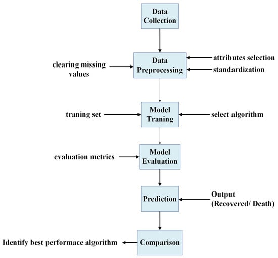
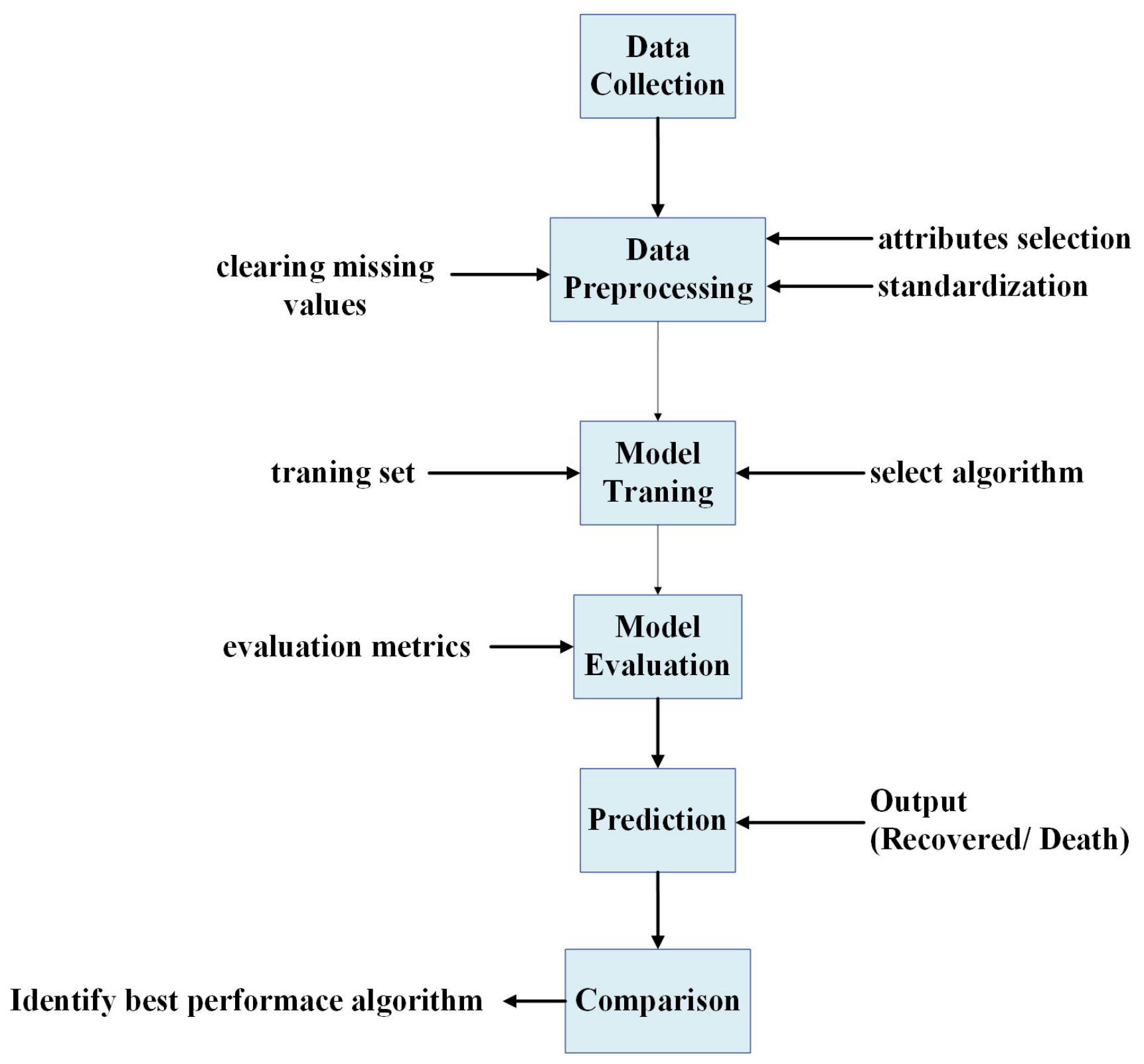
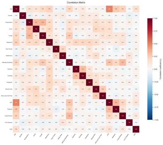
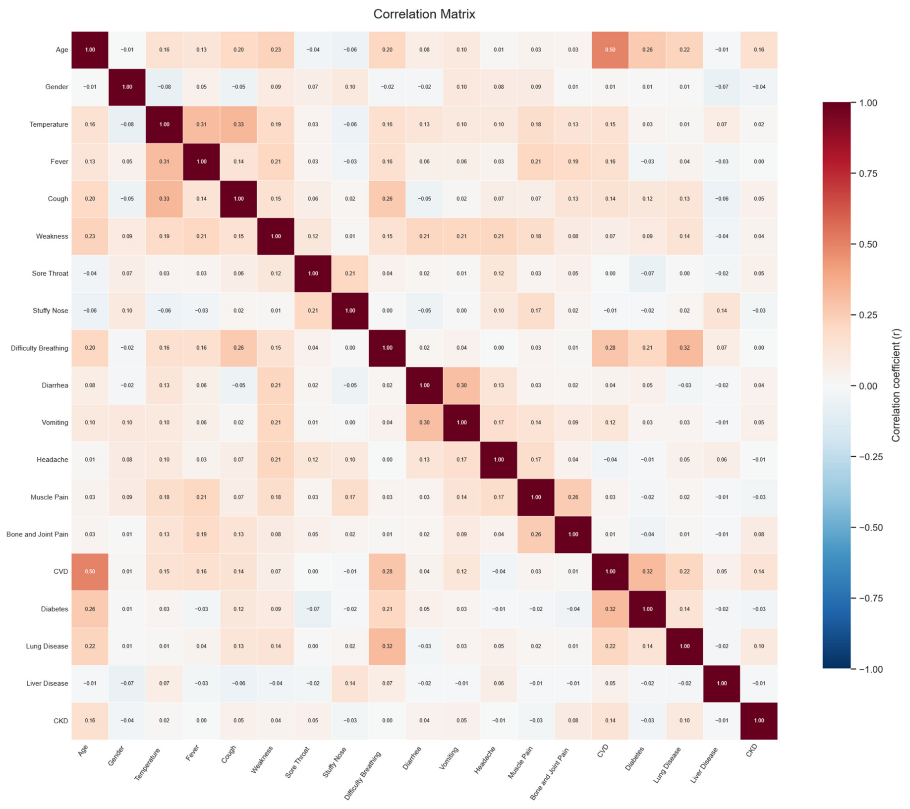
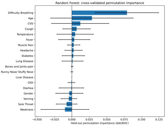
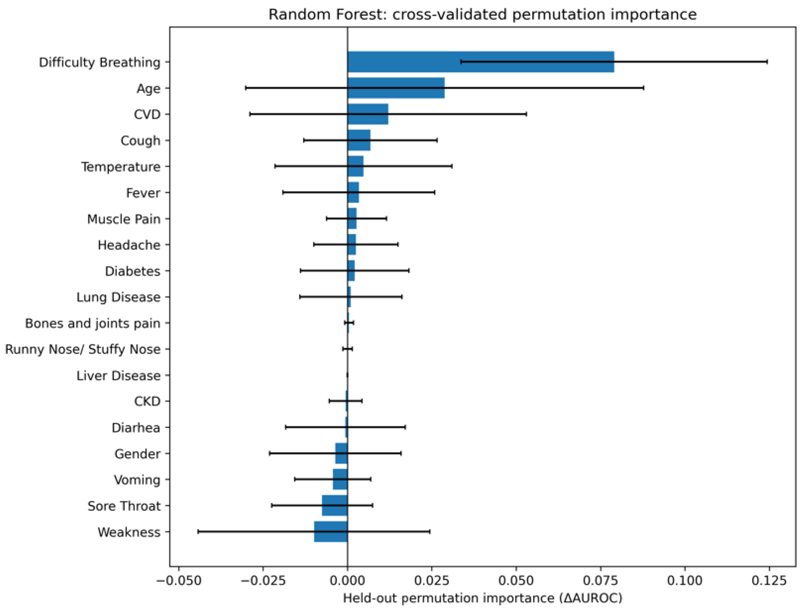
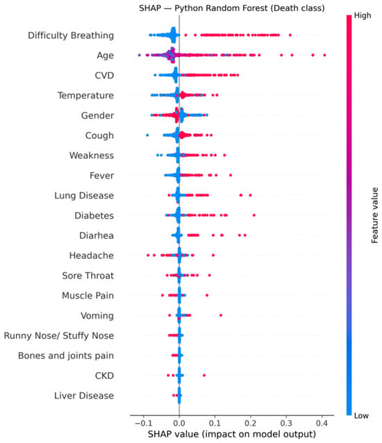
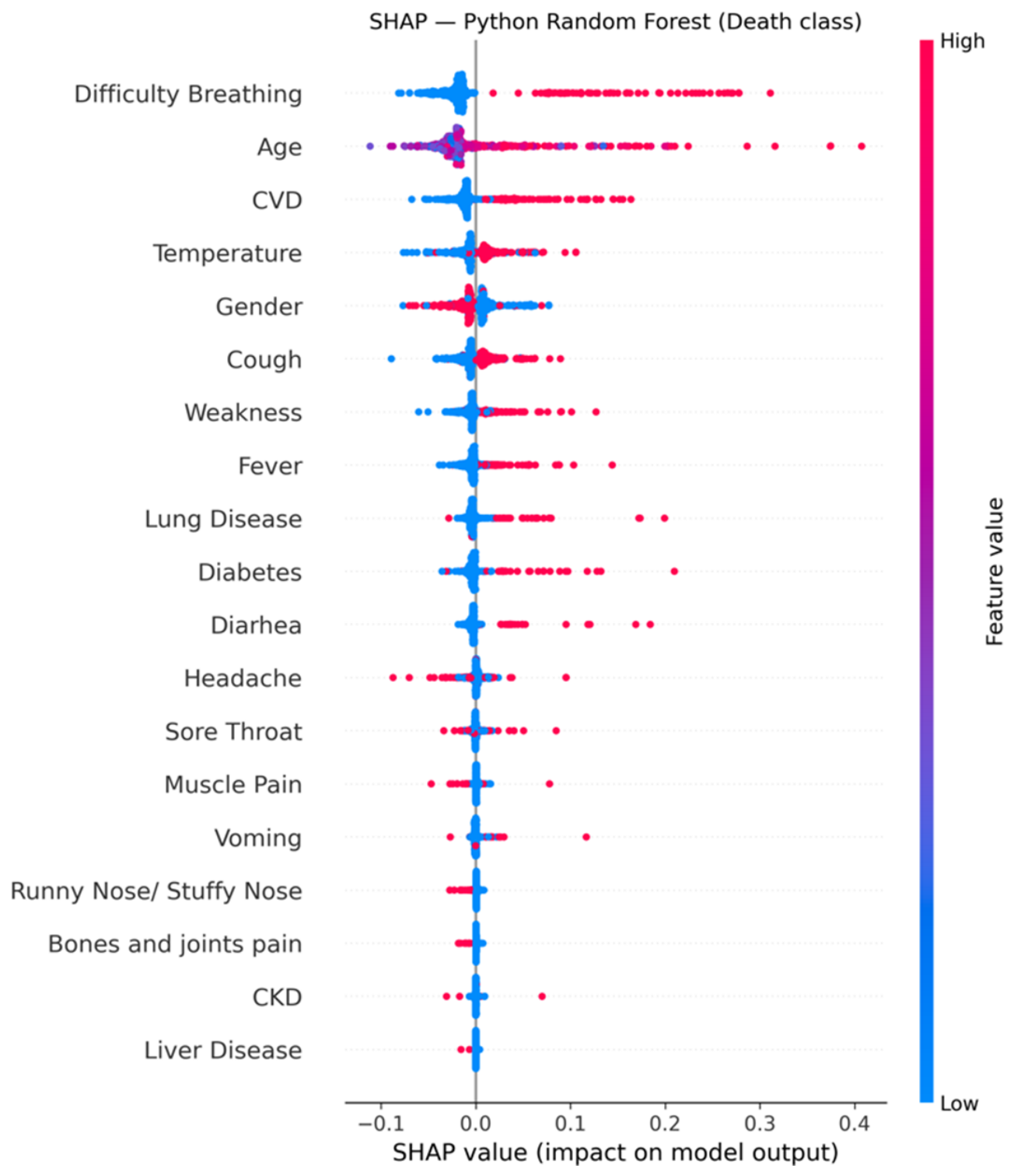
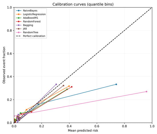
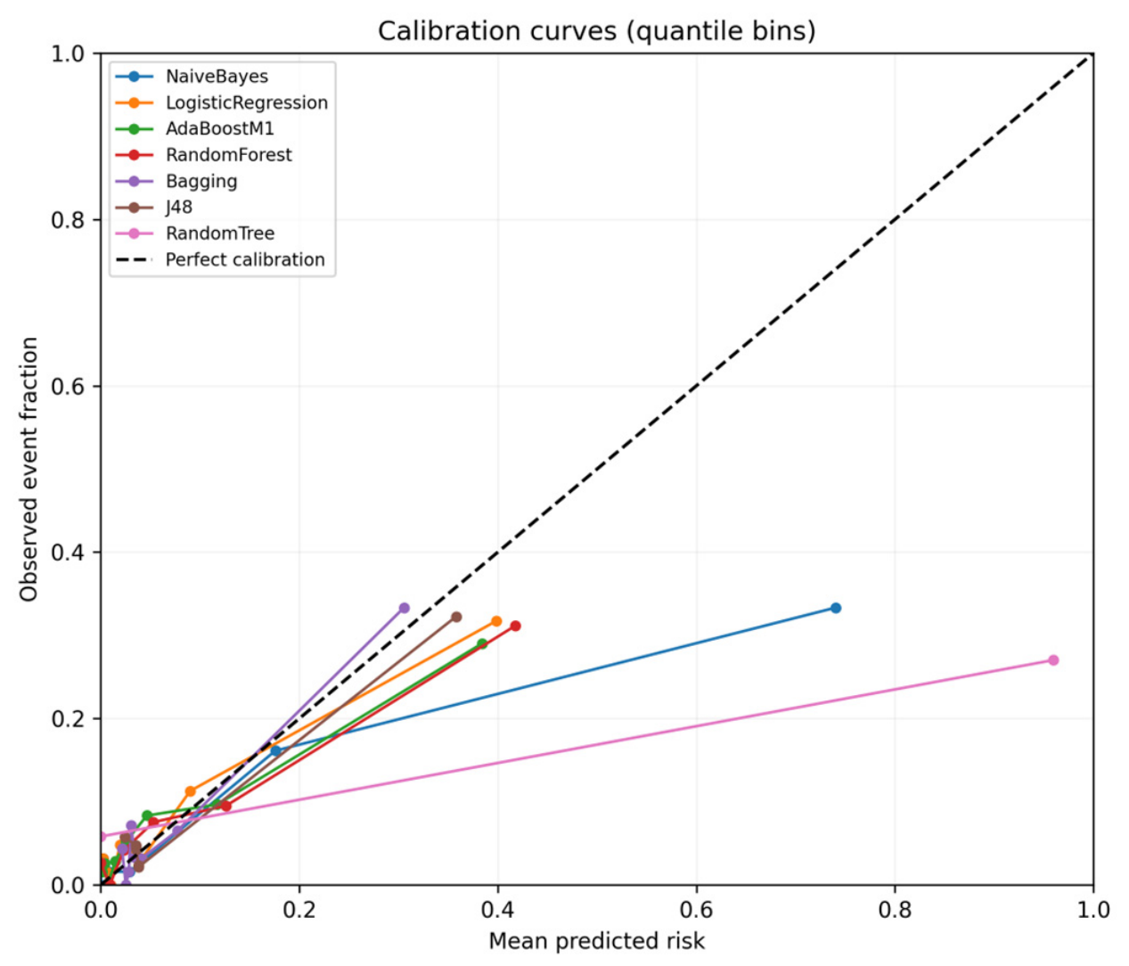
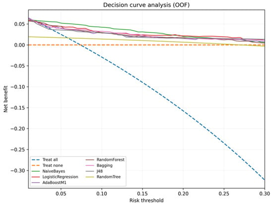
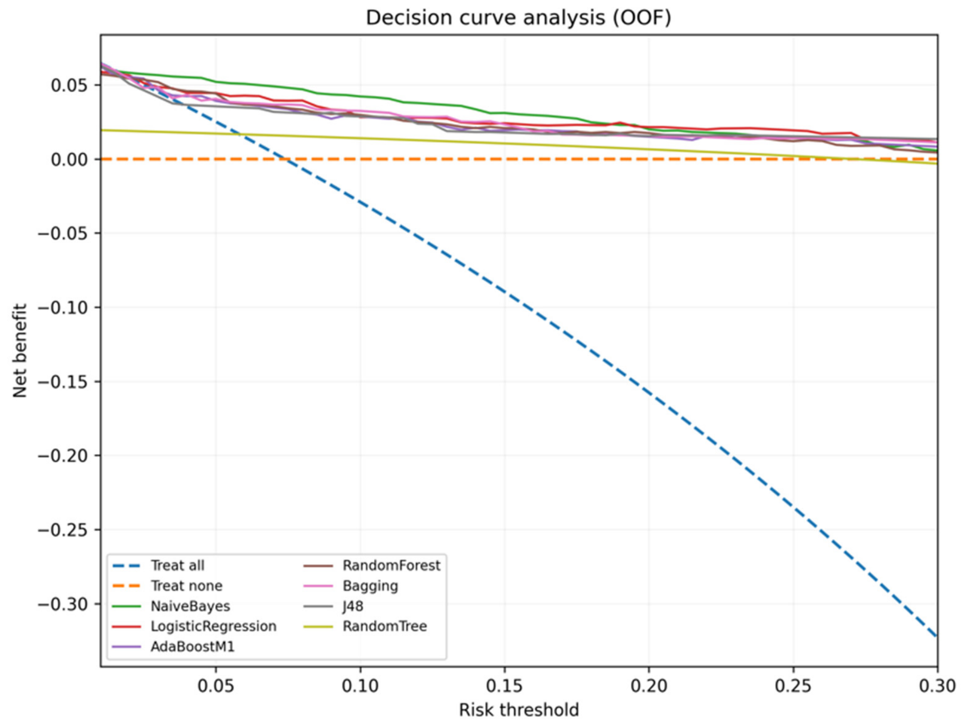

Disclaimer/Publisher’s Note: The statements, opinions and data contained in all publications are solely those of the individual author(s) and contributor(s) and not of MDPI and/or the editor(s). MDPI and/or the editor(s) disclaim responsibility for any injury to people or property resulting from any ideas, methods, instructions or products referred to in the content. |
© 2026 by the authors. Licensee MDPI, Basel, Switzerland. This article is an open access article distributed under the terms and conditions of the Creative Commons Attribution (CC BY) license.