


Abstract
Magnetic resonance imaging (MRI) and [18F]fluorodeoxyglucose positron emission tomography (FDG-PET) provide complementary structural and metabolic information for computer-aided Alzheimer’s disease (AD) classification. We propose PET-Anchored MRI Supplementation (PAMS), a PET-anchored asymmetric fusion framework that incorporates MRI-derived information through a 32→16→32 bottleneck and participant-specific root mean square (RMS) calibration. PAMS was evaluated in 554 participants from the Alzheimer’s Disease Neuroimaging Initiative using three repeats of subject-grouped five-fold outer cross-validation. It achieved an accuracy of 0.6138 ± 0.0312, a Macro-F1 of 0.6173 ± 0.0320, a balanced accuracy of 0.6240 ± 0.0385, and a Macro-AUC of 0.8060 ± 0.0258. Participant-level paired analyses demonstrated Holm-adjusted Macro-F1 improvements over the PET anchor and the capacity-matched PET + PET control, whereas differences from PET-only, late fusion, and standardized concatenation were not statistically significant after correction. The capacity-matched RMS ablation further demonstrated a significant Macro-AUC improvement, although the corresponding Macro-F1 difference was not significant. Overall, PAMS provides a capacity-constrained approach to integrating MRI-derived information into a PET-anchored representation, with statistically supported improvements over the PET anchor and a capacity-matched PET + PET control.
1. Introduction
Alzheimer’s disease (AD) is a progressive neurodegenerative disorder whose pathological changes may accumulate for years before prominent clinical symptoms appear. Mild cognitive impairment (MCI) lies between cognitively normal (CN) status and dementia; reliably distinguishing CN, MCI, and AD is therefore important for early disease detection and risk stratification [1,2,3]. With advances in medical sensor technologies and imaging systems, structural, metabolic, and molecular information acquired using different physical principles has become an important source of data for assisted diagnosis of neurodegenerative diseases. Structural magnetic resonance imaging (MRI) primarily provides information on brain morphology, gray-matter atrophy, and anatomy, whereas positron emission tomography (PET) captures signals related to brain metabolism or molecular pathology. Because structural atrophy, metabolic abnormalities, and molecular pathology in AD do not necessarily occur in synchrony, a single imaging modality typically captures only one aspect of disease progression. Joint analysis of MRI and PET, two imaging technologies with distinct signal-acquisition mechanisms, can therefore provide complementary information for AD classification [4,5,6,7].
Research on multimodal MRI/PET learning has progressed from concatenating handcrafted imaging features and regional statistics to deeper forms of representational interaction, including shared latent spaces, attention, cross-attention, Transformers, and multiscale fusion [8,9,10,11,12,13,14]. These methods strengthen joint modeling of structural and metabolic or molecular imaging information, shifting the focus from simple aggregation toward more flexible cross-modal representation learning. For MRI/PET data acquired through different imaging and sensing mechanisms, a key challenge in multimodal computer-aided diagnosis is to achieve stable and effective fusion while preserving modality-specific information.
More extensive cross-modal interaction does not necessarily make fusion more controllable. Studies of multimodal learning show that modalities can differ in information content, optimization speed, and generalization behavior, and that a stronger modality may dominate joint prediction [15,16,17,18,19,20,21,22]. Multimodal models also introduce additional parameters and representational degrees of freedom. In 3D medical-imaging tasks with limited sample sizes, observed performance changes may therefore reflect both genuine cross-modal complementarity and increased model capacity [23,24]. Comparing unimodal and multimodal performance alone cannot establish whether the second modality contributes new information or mainly adds trainable degrees of freedom.
When one modality already provides a strong baseline discriminative representation, the effect of an auxiliary modality depends not only on its supplementary information but also on the representational capacity and numerical magnitude with which that information enters the main pathway. If the auxiliary branch has degrees of freedom comparable to those of the main branch, it may learn another complete discriminative representation. If its output scale varies across subjects or training states, the same supplementary information may influence the final representation with different strengths. The amount an auxiliary modality can represent and the magnitude at which its information is injected should therefore be treated as distinct constraints.
We ask whether, when MRI and PET have unequal baseline discriminative abilities for a task, the stronger modality’s base representation can be preserved while the other modality is restricted to a cross-modal increment with controlled capacity and effective scale, yielding a multimodal biomedical image-fusion process with explicit and auditable primary and auxiliary roles.
To address the challenge of asymmetric multimodal information integration, we propose PET-Anchored MRI Supplementation (PAMS) for CN/MCI/AD classification. In this framework, PET serves as the anchor representation, while MRI contributes supplementary information through a low-dimensional correction pathway. A participant-specific RMS calibration mechanism regulates the magnitude of the MRI-derived increment relative to the PET anchor.
To examine the contributions of the individual design components, we evaluated PAMS against a PET anchor, a capacity-matched PET + PET control, and an MRI correction without RMS matching, and investigated the effects of reversing the anchoring direction and varying the bottleneck width. We further compared PAMS with unimodal classifiers and conventional fusion methods under the same CN/MCI/AD classification task.
2. Related Work
2.1. Multimodal MRI/PET Classification of Alzheimer’s Disease
Early neuroimaging-based assisted classification of AD relied mainly on handcrafted imaging features and conventional machine-learning methods. Structural MRI is commonly used to derive morphological measures such as hippocampal volume, gray-matter density, and cortical thickness, whereas PET provides regional uptake values and imaging information related to metabolism or molecular pathology. Multicentre databases such as ADNI have provided an important foundation for joint studies of MRI, PET, clinical scales, and other biomarkers [25,26,27,28]. Before deep learning became widespread, multimodal methods primarily integrated regional statistics from different modalities through feature concatenation, canonical correlation analysis, kernel learning, or ensemble classifiers.
With the development of representation learning, AD classification has shifted from handcrafted feature engineering toward data-driven deep representations. Suk et al. [8] used deep Boltzmann machines to learn hierarchical shared representations of MRI and PET, providing early evidence for the feasibility of deep multimodal learning in AD/MCI recognition. Subsequently, 3D convolutional neural networks moved neuroimaging analysis from region-level handcrafted features toward end-to-end or semi-end-to-end representations. Deep PET-only models have been used for AD diagnosis and prediction of cognitive decline [29,30], while multimodal MRI/PET models have jointly modeled complementary structural, metabolic, and molecular pathological information [31,32,33,34,35]. Accordingly, current research has shifted from whether to fuse modalities to how to fuse them more effectively and interpretably.
2.2. Deep Learning-Based MRI/PET Multimodal Fusion
The increased representational capacity of deep-learning models has shifted MRI/PET research from independent feature extraction toward cross-modal interaction. Early methods commonly concatenated high-level features or used joint mappings to construct a unified discriminative representation. Attention mechanisms were subsequently introduced to select informative features across modalities and network levels. Zhang and Shi [9] fused multilevel MRI/PET features using attention; Zhang et al. [11] further modeled cross-modal dependencies with cross-attention; and Abdelaziz et al. [14] jointly modeled cross-scale and cross-modal relationships at multiple scales. Transformers, adaptive attention, and other interaction mechanisms have further increased information-exchange flexibility between the modalities [36,37,38,39,40,41,42,43].
Existing methods have generally pursued increasingly extensive interaction, but greater interactional freedom does not necessarily make a fusion mechanism more interpretable. When MRI and PET differ in unimodal discriminative ability, symmetric concatenation, bidirectional attention, and other high-capacity mappings allow both pathways to jointly reconstruct the final representation. The resulting gains may therefore reflect genuine complementarity, additional parameter capacity, and rescaling or perturbation of the original representations. Existing methods are well suited to asking how two modalities can interact more fully but less often address how much representational freedom and what scale the second modality should have when the first is stronger. This question directly motivates our method.
2.3. Modality Imbalance and Constrained Multimodal Learning
Modality imbalance has been widely observed across multimodal-learning tasks. Previous studies show that modalities may differ substantially in information content, optimization speed, and final predictive contribution; in some cases, a stronger modality can dominate decisions during joint training [15,16,17,18,19,20,21,22]. Strategies for mitigating this problem include modality reweighting, training-process balancing, feature normalization, and adaptive modulation. Most of these methods, however, retain shared or joint representation learning as their basic paradigm. They primarily seek to balance modalities as they jointly construct a representation, rather than specifying the functional division between primary and auxiliary modalities in advance.
After primary and auxiliary roles have been defined, we focus on two further mechanistic questions: how to constrain the auxiliary modality’s representational degrees of freedom and how to set its numerical scale relative to the primary representation. Modality weighting, feature standardization, and representational-capacity constraints act at different levels and should not be treated as interchangeable. For this task, PAMS uses PET as the anchored primary pathway, restricts the degrees of freedom of the MRI correction through a low-dimensional bottleneck, and controls its relative magnitude using PET-referenced, subject-wise RMS calibration. The central contribution is therefore not a new general-purpose normalization operator but an asymmetric fusion process that jointly organizes modality roles, supplementation capacity, and injection scale.
3. Methods
3.1. Problem Definition and Overall Framework
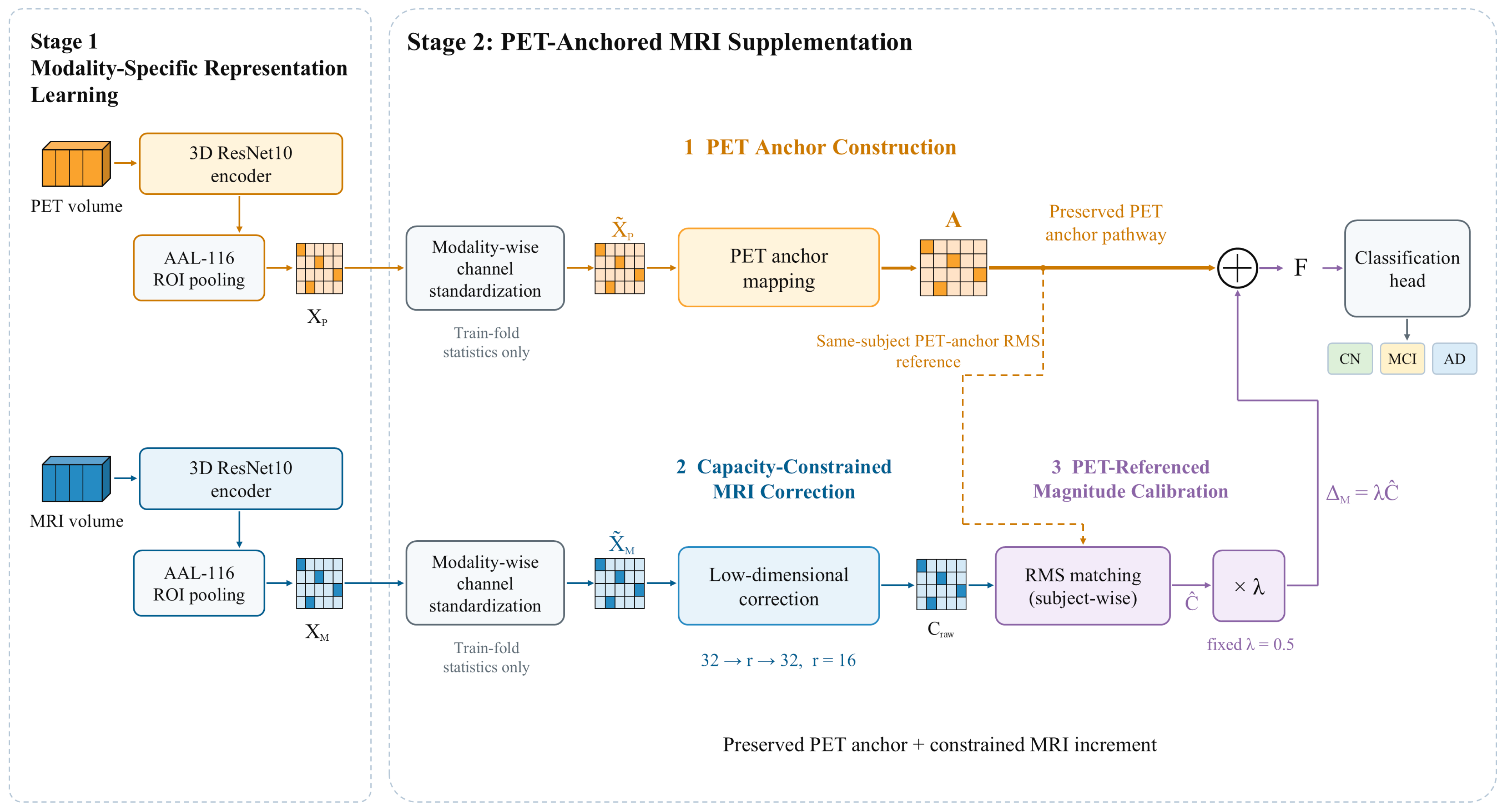
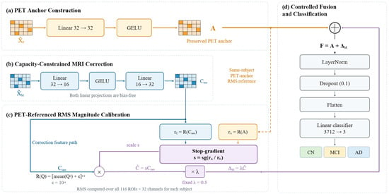
We investigate three-class classification of cognitively normal (CN), mild cognitive impairment (MCI), and Alzheimer’s disease (AD) from paired brain MRI/PET scans. For subject i, the inputs are 3D MRI and PET images from the same subject, and the model outputs predicted probabilities for the three diagnostic classes. The overall PET-Anchored MRI Supplementation (PAMS) framework is shown in Figure 1 and comprises two successive stages. Stage 1 learns modality-specific representations for MRI and PET separately and constructs regional features using a common anatomical parcellation. Stage 2 performs PET-anchored MRI incremental supplementation on fixed regional representations and produces the final classification.
Figure 1.
Overall architecture of PAMS. In Stage 1, separate 3D ResNet10 encoders and AAL-116 ROI pooling construct regional MRI/PET representations. In Stage 2, PET provides the anchoring pathway, and asymmetric fusion is performed through a capacity-constrained MRI increment calibrated in magnitude against PET, followed by classification into CN, MCI, and AD.Gold and blue denote the PET and MRI pathways, respectively. The dashed arrow indicates the subject-specific PET RMS reference, and ⊕ denotes element-wise addition.
In Stage 1, MRI and PET are processed by structurally identical but independently parameterized 3D ResNet10 encoders, which learn modality-specific representations under separate unimodal classification supervision. To ensure consistent anatomical indexing for subsequent fusion, ROI-level representations are extracted from intermediate encoder features using the AAL-116 atlas [44], yielding regional feature matrices for both modalities in the same brain-region order. Because independently trained encoders may produce different channel distributions, MRI and PET ROI features are standardized before Stage 2 using statistics estimated from the current training subset. After Stage 1, both encoders and their BatchNorm running statistics are frozen. Subsequent fusion operates only on the previously extracted fixed ROI representations, preventing Stage 2 from altering the unimodal base feature spaces.
Stage 2 organizes MRI/PET fusion as preservation of the PET-anchored representation with controlled injection of supplementary MRI information. As shown in Figure 1, standardized PET ROI features are first transformed by a trainable linear mapping to form an anchor A, which is retained as the base term of the fused representation. MRI ROI features pass through a 32 → 16 → 32 low-dimensional bottleneck to produce a raw correction Craw. Unlike methods in which both modalities jointly reconstruct a new representation, PAMS preserves the direct PET anchoring pathway and restricts MRI to an incremental correction of the base representation, explicitly distinguishing the functional roles of the two modalities.
Limiting the representational capacity of the MRI supplementation pathway alone does not determine its effective magnitude relative to the PET anchor. PAMS therefore applies PET-referenced RMS calibration to the MRI correction on a per-subject basis. Specifically, the overall magnitude of Craw is matched to the RMS of the same subject’s PET anchor, after which a fixed supplementation coefficient λ = 0.5 is applied to obtain the final MRI increment ΔM. The low-dimensional bottleneck constrains the representational capacity of the MRI correction, whereas PET-referenced RMS calibration and the fixed scaling coefficient control its overall magnitude relative to the anchor. MRI information is thus constrained in both representational capacity and numerical magnitude before entering the final fused representation.
The MRI increment ΔM and PET anchor A have the same 116 × 32 dimensions and are added elementwise to form the fused representation F. F is then processed by LayerNorm and Dropout, flattened, and passed to a linear classifier to predict CN, MCI, and AD. During Stage 2 training, the Stage-1 encoders remain fixed; only the PET anchoring mapping, MRI correction pathway, and downstream classification parameters are optimized. The complete data flow is modality-specific representation learning → anatomically aligned ROI representations → PET anchor construction → capacity-constrained MRI correction → PET-referenced magnitude calibration → incremental fusion and classification, allowing MRI information to update the PET-anchored representation as a constrained increment.
3.2. Modality-Specific Encoding and Anatomically Aligned ROI Representations
Because MRI and PET differ in imaging mechanism and intensity distribution, we use separate 3D ResNet10 encoders with identical architectures but independent parameters [45,46]. Each encoder has a base width of 32 channels and comprises a 3D convolutional stem, a max-pooling layer, and four residual stages. In Stage 1, each encoder is trained independently for CN/MCI/AD classification using global average pooling, Dropout, and a linear classification head. The aim is to obtain stable unimodal representations rather than to perform multimodal fusion. After training, the unimodal classification heads are removed, and only the encoders are retained for regional feature extraction.
Global pooling at the end of an encoder compresses the spatial dimensions and is therefore unsuitable for preserving region-level correspondence. To provide MRI and PET with a common anatomical index for subsequent fusion, we use the AAL-116 atlas to parcellate intermediate encoder features and pool features within each brain region. Repeated downsampling reduces feature-map spatial resolution, so small ROIs may lack valid support on a discrete grid at deeper feature levels. We map AAL labels to each candidate feature level, count valid positions for all 116 ROIs, and select the deepest level that retains every region as the source of ROI features. This selection criterion depends only on anatomical coverage and does not use diagnostic labels or classification performance.
Under the present network configuration, both the stem output (stage 0) and the first residual stage (stage 1) retain all 116 ROIs, whereas deeper stages contain empty ROIs. We therefore use the 32-channel feature grid from stage 1 for regional representation extraction. The AAL label map is resampled using nearest-exact nearest-neighbor interpolation to prevent mixing discrete region labels, whereas continuous images are spatially resampled using trilinear interpolation. If a candidate level contains an empty ROI, that region is not artificially filled with zeros; instead, the process falls back to the preceding valid level that covers all 116 regions. This strategy ensures one-to-one anatomical indexing between the MRI and PET regional representations.
Image preprocessing was performed using MATLAB R2023b (MathWorks, Natick, MA, USA), SPM12 r7771 (Functional Imaging Laboratory, University College London, London, UK), and CAT12.9 r2577 (Structural Brain Mapping Group, Jena University Hospital, Jena, Germany). MRI volumes underwent bias-field correction, tissue segmentation, and Fast Optimized Shooting normalization to MNI152NLin2009cAsym (113 × 137 × 113 voxels at 1.5 mm isotropic resolution). The FDG-PET images were obtained at the “Coreg, Avg, Std Img and Vox Siz, Uniform Resolution” processing level. Each PET volume was rigidly coregistered to the participant’s native MRI using six-parameter SPM registration with normalized mutual information. The MRI-derived forward deformation field was then applied to PET using trilinear interpolation, without additional smoothing.
The CAT12 tissue-label mask (wp0 > 0.5) was applied to both modalities, with voxels outside the mask set to zero and negative PET intensities clipped to zero. No additional reference-region SUVR normalization or partial-volume correction was performed. The AAL-116 labels were mapped to the same MNI space using nearest-neighbor interpolation. Before model input, volumes were resized to 96 × 112 × 96 using trilinear interpolation (align_corners = False) and standardized using positive-valued voxels. All 554 image pairs shared the same atlas grid and affine geometry. PET atlas field-of-view coverage ranged from 99.93% to 100.0%.
Let Ωr denote the set of valid positions for ROI r on the selected feature grid, and let (v,c) denote the feature for subject i and modality m at position v and channel c, where m∈ {M,P} denotes MRI and PET, respectively. The channel-wise regional mean is defined as follows:
Equation (1) yields an MRI or PET representation for each subject as a 116 × 32 matrix, where 116 corresponds to the fixed AAL brain-region order and 32 is the channel dimension of the selected feature level. The same ROI index refers to the same anatomical region in both modalities. Subsequent feature mappings operate along the channel dimension and share parameters across all ROIs. This regionalization preserves cross-modal anatomical correspondence but does not explicitly construct inter-regional connections; all 116 ROIs are retained through final fusion, without graph propagation or region selection.
Because the MRI and PET encoders are trained independently, equal feature dimensionality does not make the numerical scales of corresponding channels directly comparable. Passing the features into the fusion module without processing could allow encoder-related scale differences to affect subsequent mappings and fusion. To reduce this effect, we perform training-fold-only, channel-wise standardization separately for MRI and PET within each data split. For modality m, the standardized regional feature is defined as follows:
In Equation (2), the mean and sample standard deviation are estimated separately for each modality and feature channel using the training participants and all 116 ROIs. The denominator is lower-bounded by εs = 10−5, and the resulting training-set statistics are subsequently applied to the validation and test features.
This procedure yields standardized MRI and PET regional representations, and , which serve as inputs to the subsequent fusion module.
3.3. PET-Anchored Asymmetric Fusion Paradigm
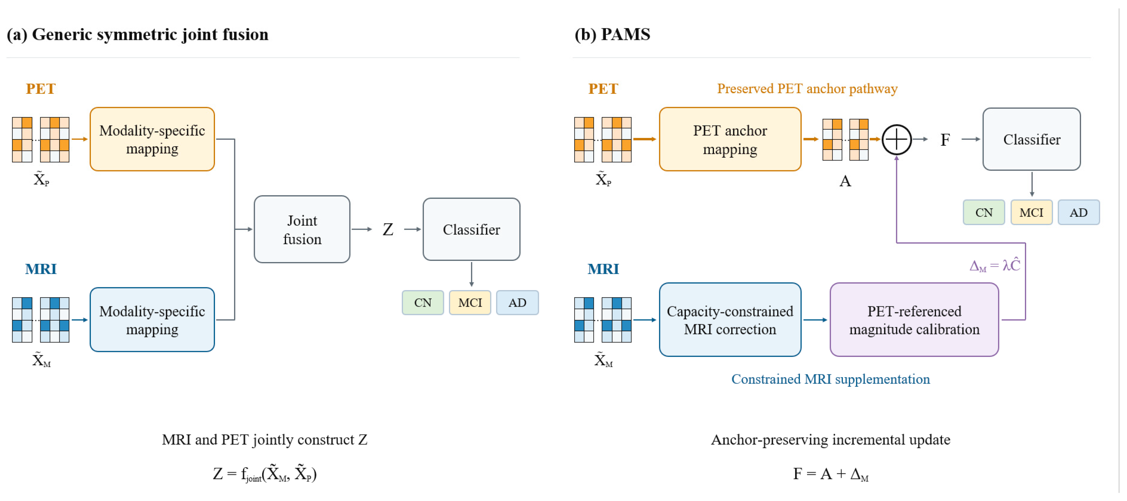
PAMS constructs the fused representation by adding a constrained MRI-derived correction to the PET anchor (Figure 2). The PET pathway provides the base representation, whereas MRI contributes an additive update through a low-dimensional bottleneck that restricts the capacity of the supplementary pathway. Participant-specific RMS matching calibrates the magnitude of this update relative to the PET anchor before fusion.
Figure 2.
(a) Symmetric joint fusion combines MRI and PET representations to produce the joint representation Z. (b) PAMS preserves the PET-anchored representation A as the base term and uses a constrained MRI correction pathway to generate the increment ΔM, updating the fused representation as F = A + ΔM.
3.4. MRI Incremental Supplementation with Controlled Capacity and Magnitude
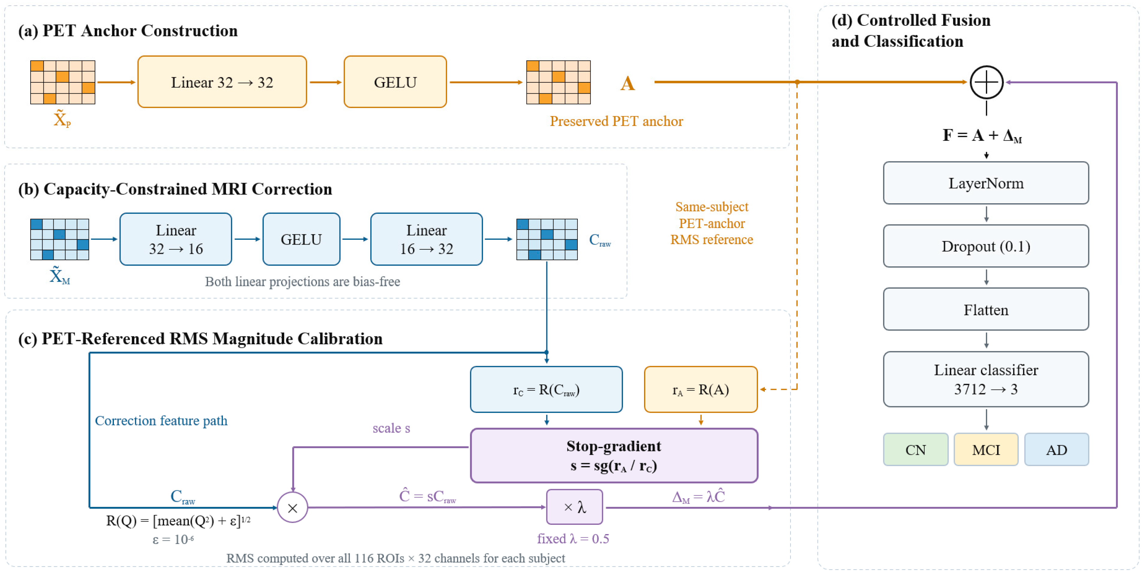
As illustrated in Figure 3, the PAMS process comprises four successive steps: PET anchor construction, low-dimensional MRI correction, PET-referenced magnitude calibration, and additive updating. Standardized PET regional features are first mapped to an anchor Ai. MRI regional features pass through a low-dimensional bottleneck to generate a raw correction Craw,i. The overall magnitude of this correction is then calibrated against the PET anchor of the same subject, yielding the MRI increment ΔM,i that is actually used in fusion.
Figure 3.
Capacity- and magnitude-constrained MRI incremental supplementation in PAMS. (a) Standardized PET regional features are mapped through a linear layer and GELU activation to form the anchor Ai. (b) MRI regional features pass through a 32 → 16 → 32 low-dimensional bottleneck to generate the raw correction Craw,i. (c) The MRI correction is calibrated against the RMS of the same subject’s PET anchor and multiplied by the fixed coefficient λ = 0.5 to obtain the applied increment ΔM,i. (d) Ai and ΔM,i are added elementwise to form the fused representation Fi.
For subject i, let denote the standardized PET regional representation. The PET pathway obtains an anchor representation through a linear mapping shared across feature channels followed by GELU activation:
Here, , , and . The same mapping parameters are applied to all 116 ROIs; feature transformation is performed only along the channel dimension, and the fixed ROI order is preserved. Ai is directly retained as the base term of the subsequent fused representation.
The MRI pathway uses a 32 → 16 → 32 low-dimensional bottleneck to generate the supplementary representation. Given the standardized MRI regional representation , the 32-dimensional features are first compressed to 16 dimensions:
They are then mapped back to the 32-dimensional feature space of the PET anchor:
Here, , , and . Neither MRI linear mapping has a bias, and both share parameters across all ROIs. Compressing the intermediate representation from 32 to 16 dimensions structurally limits the representational capacity of the MRI correction pathway. After projection back to 32 dimensions, Craw,i and Ai have the same shape and can be used to construct an incremental correction to the anchor. The MRI pathway has no independent classification head.
The low-dimensional bottleneck constrains the degrees of freedom of the MRI supplementary representation, but the overall numerical scale of Craw,i can still vary across subjects and training states. To control its effective magnitude relative to the PET anchor, PAMS calculates the root mean square magnitude over the complete regional representation matrix for each subject. For any representation , define:
Here, j and c index the ROI and feature channel, respectively. A single participant-specific RMS value is computed across all 116 × 32 elements, with εr = 10−6 included under the square root.
After calculating the RMS values of Ai and Craw,i, the PET anchor of the same subject is used as the scale reference, and the calibration factor is defined as:
Here, sg(⋅) denotes a stop-gradient operation. The scale factor si is shared across all ROIs and feature channels for the current subject, establishing an intra-subject scale relationship between the overall magnitude of the raw MRI correction and that of the corresponding PET anchor. No gradient is propagated through the RMS ratio during backpropagation; si is treated as a constant determined by the current forward pass during subsequent scaling, while the classification loss can still update the MRI correction-path parameters through Craw,i.
The calibrated MRI correction and the increment used in fusion are defined as follows:
Here, denotes the MRI correction after PET-referenced magnitude matching, and the fixed coefficient λ controls the overall proportion of this correction entering the anchor pathway. Because the same si is shared by all representational elements for a subject, the process changes only the overall scale of Craw,i; it does not alter the signs or relative magnitudes among its ROIs and feature channels.
After capacity limitation and magnitude calibration, the MRI increment and PET anchor are added elementwise at the corresponding ROIs and feature channels to form the final fused representation:
Here, . In this representation, the PET anchor is directly retained as the base term in Fi, whereas MRI information contributes to updating the anchor through the constrained increment.
When the numerical-stability term is negligible relative to representation energy and the relevant representations are non-degenerate, the above scale-matching relationship yields:
When the numerical-stability term can be neglected, the subject-level overall RMS of the MRI increment is approximately proportional to that of the PET anchor, with the ratio determined by λ. This constraint applies to the complete 116 × 32 representation matrix and does not independently rescale individual ROIs, feature channels, or elements. The sign and relative magnitude of local corrections are therefore determined by the internal feature structure of Craw,i.
RMS matching scales the MRI-derived increment relative to the magnitude of the learned PET anchor. Consequently, participants with larger anchor RMS values receive proportionally larger MRI increments for a given λ. The reference is the learned PET feature tensor after training-fold standardization and projection, whose RMS provides the numerical scale for calibrating the supplementary contribution.
3.5. Two-Stage Training and Classification Optimization
PAMS uses two-stage training to separate unimodal feature learning from multimodal fusion optimization. In Stage 1, two structurally identical but independently parameterized 3D ResNet10 encoders are trained separately for MRI and PET, each under CN/MCI/AD classification supervision. After this stage, the unimodal classification heads are no longer used; only the encoders are retained to generate ROI representations indexed by the AAL-116 atlas. This design means that Stage 2 performance changes primarily reflect the effect of the fusion module on fixed base representations, rather than simultaneous changes to the unimodal feature spaces through end-to-end joint fine-tuning.
Stage 2 takes the frozen MRI and PET ROI representations as input and trains only the PET anchoring mapping, MRI incremental supplementation pathway, and final classification module. Both Stage-1 encoders remain in evaluation mode, and their BatchNorm running means and variances are not updated. ROI representations for each data split are extracted and cached after Stage 1, ensuring that different Stage-2 configurations within the same outer fold use identical base inputs and reducing additional comparison bias from stochastic feature extraction.
For subject i, let denote the fused representation. LayerNorm is first applied to the 32-dimensional feature vector of each ROI, followed by Dropout with a probability of 0.1. The regional representations are then flattened in the fixed AAL-116 ROI order to a 116 × 32 = 3712-dimensional vector. A linear classifier maps the flattened features to a three-dimensional output space and produces logits for CN, MCI, and AD. Given classifier output , predicted probabilities are obtained as pi = Softmax(zi). The fixed ROI order is maintained during flattening, so each brain region occupies a defined position in the final classification vector.
Because the numbers of CN, MCI, and AD samples differ, Stage 2 uses class-weighted cross-entropy as the classification objective. Let the current training subset contain Ntr samples, of which Nk belong to class k; the class weight is defined as wk = Ntr/(3Nk). For a training batch of B samples, the classification loss is defined as follows:
Here, yi ∈ {1,2,3} denotes the true class of sample i, and is the predicted probability assigned to its true class. Class weights are computed only from the class distribution in the current training subset and remain fixed during the corresponding training process. Validation and outer-test labels are not used to estimate these weights.
Trainable Stage-2 parameters include the PET anchoring mapping parameters WA and bA, MRI bottleneck parameters Wdown and Wup, LayerNorm affine parameters, and the final linear classifier parameters. RMS calculation, the stop-gradient ratio, the fixed supplementation coefficient λ = 0.5, and additive fusion introduce no additional trainable parameters. Gradients of the classification loss propagate through the PET anchoring pathway, MRI correction pathway, and classification module, whereas the frozen MRI and PET encoders are not updated in Stage 2.
The RMS ratio is computed once per participant across the full ROI-by-channel matrix, whereas LayerNorm is applied independently within each ROI across its 32 channels after the PET anchor and MRI increment are added. Ignoring the numerical stabilizer, the summed representation can be expressed as the PET-anchor RMS multiplied by a combination of unit-RMS PET and MRI features, weighted by 1 and λ, respectively. Although LayerNorm largely removes this common scale, the relative weighting of the two modality-specific components can still alter the resulting channel pattern. Thus, the audited ratio quantifies the MRI increment before LayerNorm rather than the magnitude of the post-normalization representation.
Stage 2 uses the AdamW optimizer with an initial learning rate of 1 × 10⁻³, weight decay of 1 × 10⁻⁴, and batch size of 8; the gradient norm is clipped at 5. Training runs for at most 100 epochs. The model with the best validation Macro-F1 is retained, and training is stopped early if the metric does not improve for 15 consecutive epochs.
3.6. Dataset and Experimental Protocol
Paired T1-weighted MPRAGE MRI and [18F]FDG-PET scans were obtained from ADNI [25,26,27,28]. For each participant, the MRI–PET acquisition pair with the shortest interval within 30 days was selected, with one pair retained per participant. Seven of the 561 shortlisted participants had no processed PET record corresponding to the selected MRI acquisition; alternative PET acquisitions obtained 180–192 days apart were not substituted. The final cohort comprised 554 participants (193 CN, 256 MCI, and 105 AD), including 172 EMCI and 84 LMCI participants classified as MCI. The median absolute MRI–PET acquisition interval was 8 days (IQR, 1–18; range, 0–30 days).
The MRI and PET export records were concordant for the imaging-download Group field, which was used to define the training labels. As a separate retrospective diagnostic reference, the dated DXSUM record closest to the MRI–PET acquisition midpoint was identified for each participant. These reference visits comprised ADNI1 (n = 85), ADNI-GO (n = 30), and ADNI2 (n = 439). The retrospective labels differed from the imaging-download labels for 38 participants. These reference labels were not used to relabel the cohort.
For clinical characterization, MMSE and global CDR values were obtained from the nearest valid dated records within 90 days of the MRI–PET acquisition midpoint. Education was obtained from the nearest valid demographic record without a temporal restriction. APOE ε4 carrier status was defined as the presence of at least one ε4 allele.The demographic and clinical characteristics of the final cohort are summarized in Table 1.
Table 1.
Demographic and clinical characteristics of the final ADNI MRI/FDG-PET cohort.
Group differences in MMSE, global CDR, and education were assessed using Kruskal–Wallis tests, whereas APOE ε4 carrier status was compared using Pearson’s chi-square test. Holm correction was applied across the four comparisons. The sample sizes and APOE denominators reflect the availability of corresponding records, and dashes indicate variables for which no inferential p value is reported.
Model evaluation used subject-grouped, class-stratified, three repeats of five-fold outer cross-validation, yielding 15 outer-test folds. In each repeat, every participant appeared in the outer test set exactly once. The corresponding outer-training data were further divided into training and validation subsets for parameter learning, model selection, and early stopping. Outer-test data remained fully isolated throughout training for that fold and were not used to estimate standardization statistics, update model parameters, select models, or trigger early stopping. The three repeats used random seeds 0, 1, and 2. This design primarily controlled subject-level data leakage and used repeated partitioning to assess sensitivity to data splits.
Within each outer fold, all Stage-2 configurations used the same Stage-1 encoder cache, training-derived standardization statistics, model-selection criterion, and random-seed policy. The default bottleneck dimension was set to r = 16 before the outer-test sensitivity analysis comparing r = 8, 16, and 32. The bias-free 32→16→32 correction contains 1024 trainable weights; together with the PET projection, its parameter count matches the 2080 projection parameters of Linear(64,32) in standardized concatenation. The fixed coefficient λ = 0.5 scales the applied MRI increment to approximately one-half of the PET-anchor RMS before addition.
The PET anchor consists of the Stage-2 PET pathway and classifier. In the capacity-matched PET + PET control, PET features are supplied to both the anchor and correction pathways. The no-RMS control retains the MRI bottleneck and the fixed multiplier λ = 0.5 but allows the correction projection to learn its output scale freely; consequently, the multiplier alone does not constrain the correction-to-anchor RMS ratio. Standardized concatenation combines the separately standardized MRI and PET features (64 channels) and projects them to 32 dimensions using a linear layer followed by GELU. All configurations share the same downstream LayerNorm, dropout, and linear classifier.
The anchoring-direction variant exchanges the functional roles of MRI and PET. MRI regional representations form the anchor, while PET regional representations generate the supplementary term through a 32 → 16 → 32 correction pathway, calibrated against the subject-level RMS of the corresponding MRI anchor. This configuration uses the same fixed supplementation coefficient λ = 0.5, LayerNorm, Dropout, and classifier as PAMS. Bottleneck-capacity variants retain the PET anchoring pathway, MRI supplementation pathway, and RMS calibration, but vary only the intermediate bottleneck dimension r ∈ {8,16,32}. The default PAMS configuration uses r = 16; r = 8 provides a lower-dimensional supplementary representation, whereas r = 32 keeps the intermediate and input dimensions equal. All other network structures and training conditions were held constant.
The MRI-only and PET-only classifiers were trained independently on their respective 3D volumes. In late fusion, the two softmax probability vectors were averaged with equal weights for each aligned participant and outer fold, and the class with the highest averaged probability was selected. PET-only serves as a standalone unimodal baseline, whereas the PET anchor represents a component-level control based on frozen PET ROI features in Stage 2.Six internal comparisons were prespecified for paired statistical analysis: PAMS versus the PET anchor, the capacity-matched PET + PET control, the MRI correction without RMS matching, PET-only, late fusion, and standardized concatenation.
All experiments were implemented using Python 3.11.15 and PyTorch 2.6.0 and run on an NVIDIA GeForce RTX 4060 GPU(NVIDIA Corporation, Santa Clara, CA, USA) with CUDA 12.4. Major dependencies included scikit-learn 1.9.0, NumPy 2.4.6, and SciPy 1.17.1. All Stage-2 configurations were trained, evaluated, and profiled in the same software and hardware environment to minimize implementation-related differences in the comparisons.
3.7. Evaluation Metrics and Statistical Analysis
Macro-F1 was prespecified as the primary evaluation metric. We also report Accuracy, BAC, and one-vs-rest Macro-AUC. Accuracy measures overall classification correctness. Macro-F1 is the unweighted mean of the F1-scores for CN, MCI, and AD and provides a class-balanced precision–recall assessment. BAC is the unweighted mean recall across the three classes. Macro-AUC is the macro-average of the three one-vs-rest ROC-AUC values and assesses probability-ranking ability across classes [47]. Metrics across 15 outer-test folds are summarized as mean ± SD to describe average performance and variability across splits and repeats; the folds are not treated as independent statistical samples.
For the six internal comparisons, participant-level out-of-fold (OOF) predictions were aligned by participant and repeat, and participants were resampled with replacement [48]. We performed 10,000 paired bootstrap resamples using NumPy’s default_rng with seed 0. All three OOF records for each sampled participant were retained together, and identical participant indices were applied to both methods. Macro-F1, BAC, and Macro-AUC were recalculated from the pooled records within each resample. The effect size was defined as PAMS minus the corresponding comparator, and the 95% percentile confidence interval was obtained from the 2.5th and 97.5th percentiles of the bootstrap differences. The empirical two-sided p value was calculated as twice the smaller of the proportions of differences ≤ 0 and ≥0, capped at 1. Holm adjustment was applied across the six internal comparisons separately for each metric [49]. The confidence intervals are unadjusted, whereas fold-level means and standard deviations describe variability across the 15 outer-test folds.
Class-level analyses also used OOF predictions. Each participant received one outer-test prediction in each of the three repeats; we averaged the three OOF probability vectors for each participant to obtain a single subject-level consensus OOF probability. A row-normalized confusion matrix, class-level precision, recall, F1-score, and one-vs-rest ROC-AUC were then calculated across the 554 participants. This analysis characterizes diagnostic-class differences and major misclassification patterns and is not treated as a new test set independent of outer cross-validation.
For each outer fold, participant-level RMS values of the PET anchor, raw MRI correction, and applied MRI increment were calculated for both the validation split and the corresponding outer-test set. The participant-level correction-to-anchor RMS ratios were then averaged within each split. The validation-set calibration audit is reported in Section 4.5, while the corresponding outer-test results are provided in Table S8. The pre-calibration ratio quantifies the natural magnitude of the raw MRI correction relative to the PET anchor, whereas the post-calibration ratio quantifies the magnitude of the MRI increment incorporated into the fused representation. The pre-calibration ratio describes the natural scale of the MRI correction relative to the PET anchor, whereas the post-calibration ratio describes the relative magnitude of the MRI increment entering the fused representation. When the numerical-stability term is negligible, the calibrated ratio should theoretically approach the fixed supplementation coefficient. This audit directly tests implementation consistency of the magnitude-control mechanism rather than inferring it from classification metrics.
Computational complexity was evaluated in terms of model capacity, primary linear computation, and runtime. For the main Stage-2 configurations, we measured trainable parameters, linear multiply–accumulate operations (MACs), profiler FLOPs, single-sample inference time, and peak GPU memory. Because all configurations share the same frozen Stage-1 ROI representations, complexity was measured only for Stage 2 to attribute computational costs directly to the fusion structures.
4. Experiments
4.1. Comparison with Representative MRI/PET Multimodal AD Classification Methods
Table 2 presents the fold-level mean and standard deviation of the four evaluation metrics for Zhang Transformer [12], MDL-Net [13], camAD [43], MMSDL [14], and the MRI-only, PET-only, late-fusion, and standardized-concatenation baselines. Comparisons with the four external methods are descriptive, whereas participant-level paired statistical analyses are conducted for the internal controls and conventional baselines with the corresponding results reported in Section 4.3.
Table 2.
Quantitative comparison of PAMS with representative MRI/PET multimodal methods for AD classification (15 outer-test folds; mean ± SD).
PET-only achieved a higher mean Macro-F1 than MRI-only across the outer-test folds (0.5831 versus 0.4830). Importantly, the PET anchor is distinct from the standalone PET-only classifier, as it serves as a component-level control within the Stage-2 fusion architecture using frozen PET ROI features. Its mean Macro-F1 was 0.5638.
Among the evaluated methods, PAMS achieved the highest fold-level mean Accuracy, Macro-F1, and BAC, whereas MMSDL yielded the highest mean Macro-AUC (0.8091 versus 0.8060 for PAMS). The difference in mean Macro-F1 between PAMS and MMSDL was 0.0065.
4.2. Mechanistic Controls and Ablation Analyses
Table 3 summarizes the fusion controls, the reversed anchoring direction, and the bottleneck-width sensitivity comparison under the evaluated protocol.
Table 3.
Mechanistic controls, anchoring direction, and bottleneck-capacity sensitivity analyses for PAMS (15 outer-test folds; mean ± SD).
PAMS and the capacity-matched PET + PET control share the same correction architecture and Stage-2 parameter count. Despite this structural equivalence, PAMS achieved a higher fold-level mean Macro-F1. Participant-level paired analysis further confirmed a significant improvement over the PET + PET control (Δ = 0.0379, 95% CI, 0.0126–0.0642, Holm-adjusted p = 0.0130). This finding supports the contribution of MRI-derived supplementary information beyond the effect of introducing an additional correction pathway with matched capacity.
The largest fold-level performance advantage of PAMS over the freely scaled no-RMS control was observed for Macro-AUC. The participant-level paired analysis in Section 4.3 evaluates the corresponding differences in classification performance, whereas the RMS audit in Section 4.5 independently verifies whether the prescribed magnitude constraint is achieved.
Across all four evaluation metrics, the MRI-anchored configuration yielded lower fold-level means than the PET-anchored configuration, indicating that PET anchoring was more favorable within the evaluated fusion architecture.
Among the evaluated bottleneck dimensions (r = 8, 16, and 32), r = 16 yielded the highest fold-level means across all four evaluation metrics. These results indicate that the selected intermediate dimension provides a favorable balance in the representational capacity of the MRI correction pathway within the evaluated configurations.
4.3. Subject-Level Paired Statistical Results
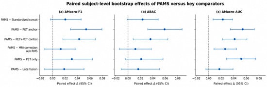
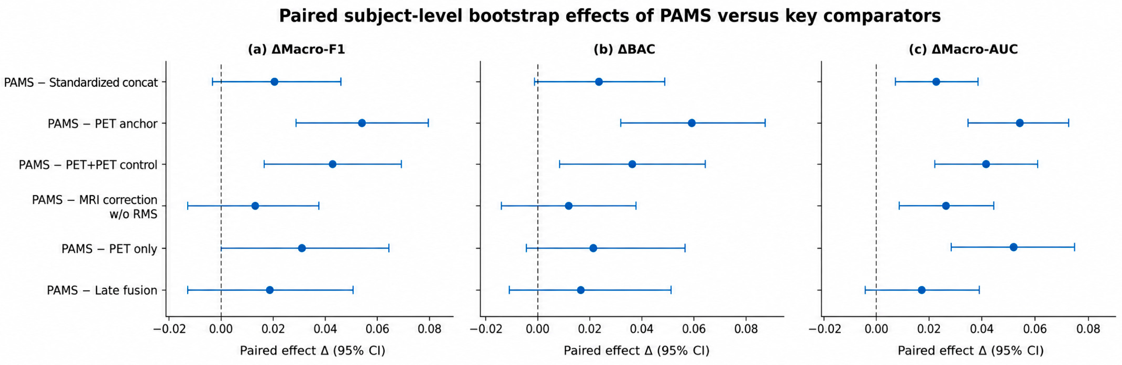
Participant-level paired effects are summarized in Table 4 and Figure 4, with Macro-F1 designated as the primary endpoint.
Figure 4.
Forest plot of subject-level paired effects of PAMS relative to key comparators. Points indicate Δ = PAMS − Comparator; horizontal lines indicate 95% confidence intervals; the vertical dashed line indicates Δ = 0. Positive values indicate a higher metric for PAMS.
Table 4.
Participant-level paired effects of PAMS relative to internal comparators. Δ denotes the difference between PAMS and the corresponding comparator. Bracketed values indicate unadjusted 95% bootstrap percentile confidence intervals. p values are adjusted using Holm’s method separately within each metric.
PAMS demonstrated a positive participant-level paired Macro-F1 difference relative to the PET anchor (Δ = 0.0501, 95% CI, 0.0236–0.0775), with no bootstrap resamples falling in the smaller empirical tail. A significant improvement was also observed relative to the capacity-matched PET + PET control (Δ = 0.0379, 95% CI, 0.0126–0.0642, Holm-adjusted p = 0.0130). Together, these findings provide evidence that MRI-derived supplementation improves Macro-F1 within the PET-anchored architecture and contributes beyond the addition of a capacity-matched correction pathway.
After Holm adjustment, the paired Macro-F1 differences between PAMS and PET-only, late fusion, and standardized concatenation were not statistically significant (adjusted p = 0.1608, 0.5856, and 0.2682, respectively). The difference between PAMS and the no-RMS control was also nonsignificant (adjusted p = 0.5856).
PAMS also achieved its largest paired BAC improvement relative to the PET anchor (Δ = 0.0534, 95% CI, 0.0262–0.0814). The remaining BAC comparisons did not reach statistical significance after Holm adjustment.
For the secondary Macro-AUC endpoint, PAMS demonstrated significant participant-level paired improvements over standardized concatenation (Δ = 0.0184, 95% CI, 0.0059–0.0315, Holm-adjusted p = 0.0108) and the no-RMS control (Δ = 0.0220, 95% CI, 0.0093–0.0348, Holm-adjusted p = 0.0012).
4.4. Class-Level Classification Performance and Error Patterns
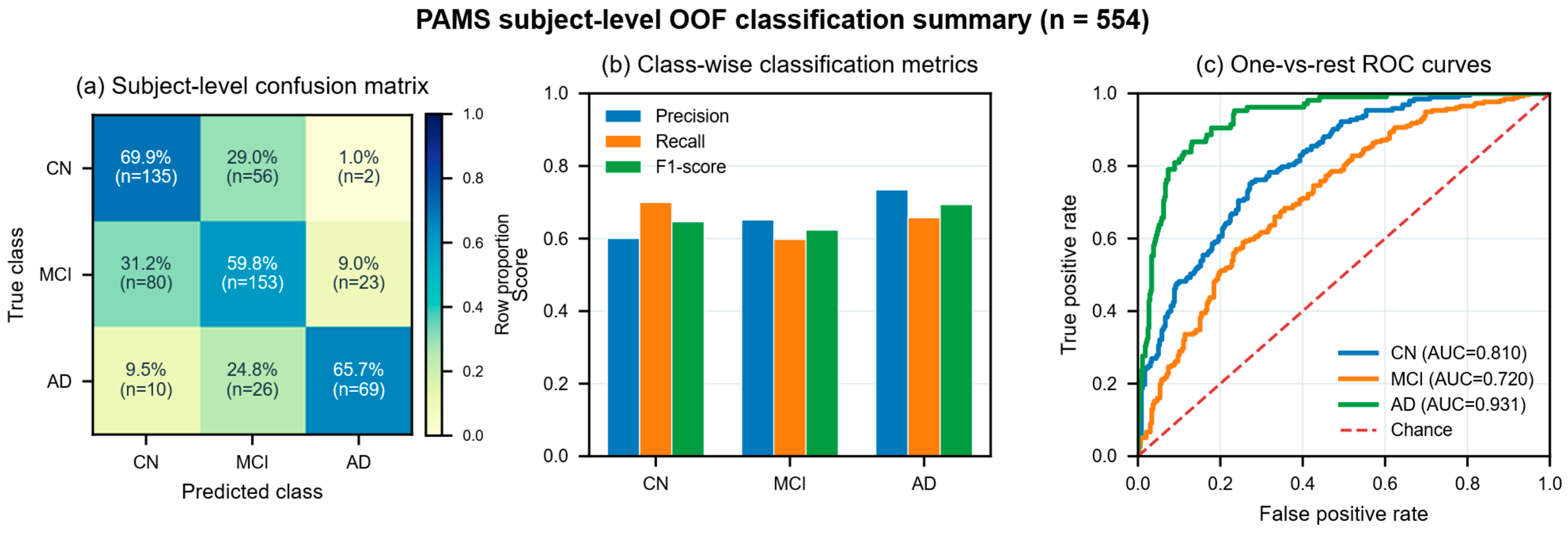
Figure 5 summarizes participant-level consensus predictions obtained by averaging the three repeat-specific OOF probability vectors for each participant. Among the three diagnostic classes, MCI exhibited the lowest recall (0.5977) and F1-score (0.6232).
Figure 5.
Subject-level consensus OOF classification results for PAMS. For each participant, the outer-test predicted probabilities from the three repeats were averaged to calculate (a) a row-normalized confusion matrix; (b) precision, recall, and F1-score for CN, MCI, and AD; and (c) one-vs-rest ROC curves and AUCs.
Of the 256 MCI participants, 153 were correctly classified as MCI, whereas 80 were classified as CN and 23 as AD. The recall values for CN and AD were 0.6995 and 0.6571, respectively. Direct confusion between CN and AD involved 12 participants.
The class-specific one-vs-rest AUCs were 0.8101 for CN, 0.7204 for MCI, and 0.9313 for AD.
4.5. RMS Magnitude Calibration Audit
As shown in Figure 6, across the 15 validation splits, the pre-calibration fold-mean RMS ratio between the raw MRI correction and the PET anchor ranged from 0.0984 to 0.5513 (range, 0.4529; SD, 0.1463). This substantial variability indicates that the uncalibrated MRI correction did not maintain a consistent magnitude relative to the PET anchor across data splits. Participant-specific RMS matching was therefore introduced to regulate the relative contribution of MRI-derived information to the fused representation.
Following participant-specific RMS matching, the applied correction-to-anchor RMS ratio was confined to 0.49994–0.50000, closely matching the prespecified supplementation coefficient of λ = 0.5. The ratio range decreased from 0.4529 before calibration to 0.00006 after calibration, while the across-fold standard deviation decreased from 0.1463 to 0.00002. These results demonstrate that PAMS consistently enforces the prespecified relative magnitude of the MRI increment across validation splits.
Figure 6.
RMS magnitude-calibration audit for PAMS. (a) Pre-calibration raw correction-to-anchor RMS ratios across the 15 validation splits; (b) deviations of the post-calibration applied ratio from the λ = 0.5 target; and (c) the RMS values of the PET anchor, raw MRI correction, and applied correction in each validation split.
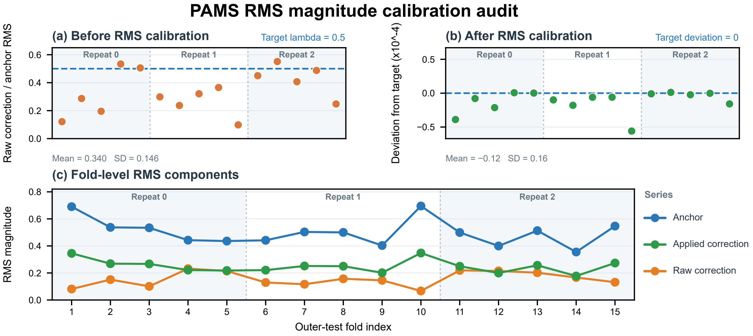
In terms of across-fold dispersion, RMS matching substantially reduced variation in the relative scale between the correction and the anchor, but it did not eliminate differences in their absolute representation magnitudes. The absolute RMS values of the PET anchor and applied correction still had across-fold standard deviations of 0.0966 and 0.0483, respectively, whereas their relative ratio remained stable near 0.5. Thus, the mechanism controls the proportion of the MRI increment relative to the PET anchor rather than imposing a common absolute-magnitude normalization across samples or data splits.
In terms of absolute magnitude, the raw MRI correction had a mean RMS of 0.1553. After calibration and multiplication by the fixed coefficient, the applied correction had a mean RMS of 0.2499, approximately half of the mean PET-anchor RMS of 0.4999. This result closely matched the theoretical setting of λ = 0.5, showing that magnitude calibration can accurately constrain the overall strength of the auxiliary branch in the main pathway while preserving absolute representation differences between samples.
Across the 15 corresponding outer-test sets, the fold-mean correction-to-anchor RMS ratio ranged from 0.1022 to 0.5544 before calibration and from 0.49995 to 0.50000 after calibration (Table S8). This close agreement with the prespecified value of λ = 0.5 demonstrates that the calibration mechanism consistently maintains the intended relative magnitude in held-out data.
Compared with the MRI correction without RMS matching, PAMS achieved higher fold-level means for Accuracy, Macro-F1, BAC, and Macro-AUC, with differences of 0.0111, 0.0083, 0.0093, and 0.0205, respectively. Participant-level paired analysis further demonstrated a significant Macro-AUC improvement (Δ = 0.0220, 95% CI, 0.0093–0.0348, Holm-adjusted p = 0.0012). Although the paired differences in Macro-F1 and BAC were also positive, they did not reach statistical significance after Holm correction.
4.6. Computational Complexity Analysis
The model sizes and computational costs of the main Stage-2 configurations are reported in Table 5. PAMS contains 13,283 trainable parameters and 248,704 linear MACs, exactly matching PET + PET control and MRI correction w/o RMS. PET anchor contains 12,259 parameters and 129,920 linear MACs, so adding the MRI correction pathway increases the number of trainable parameters by only 1024. Standardized concat also contains 13,283 parameters and 248,704 linear MACs. These settings provide good model-size comparability between PAMS and the key mechanistic controls.
Table 5.
Parameter counts and computational complexity of the main Stage-2 configurations. All configurations share the same frozen Stage-1 ROI representations; therefore, the complexity reported here reflects Stage 2 only. Inference time is reported in ms/sample.
The Stage-2 profiler FLOPs ranged from 0.516 to 0.531 MFLOPs across the five configurations in Table 5.
Stage-2 inference time remained below 1 ms per sample across all five configurations.
5. Discussion
These findings support the central premise of PAMS: MRI-derived information can improve a PET-anchored representation when incorporated through a capacity-constrained and magnitude-calibrated correction pathway. The capacity-matched PET + PET comparison is particularly informative because it retains the same correction structure and Stage-2 parameter count while changing the source of the supplementary features. PAMS achieved a significantly higher participant-level Macro-F1 in this comparison, supporting the contribution of MRI-derived information beyond the effect of introducing an additional correction pathway. Furthermore, PAMS yielded the highest fold-level mean Accuracy, Macro-F1, and BAC among the evaluated methods. Although the paired Macro-F1 differences relative to PET-only, late fusion, and standardized concatenation were not statistically significant after Holm adjustment, the significant Macro-AUC improvement over standardized concatenation provides additional evidence of improved class-ranking performance.
Misclassification of 80 of the 256 MCI participants as CN identifies an important limitation in the model’s sensitivity to early cognitive impairment. Although PAMS achieved higher CN recall, its MCI recall was lower than that of both simple fusion baselines (Table S7). This class-specific trade-off is particularly relevant to early-impairment classification, because aggregate discrimination metrics may obscure MCI cases incorrectly assigned to the cognitively normal category. Nevertheless, the results provide evidence for the methodological value of the proposed fusion strategy within the evaluated cohort, while its clinical effectiveness requires further validation in dedicated clinical settings.
PAMS requires paired MRI and PET inputs, as do late fusion and standardized concatenation. Compared with PET-only classification, its application additionally depends on MRI availability, while the cost and accessibility of PET remain practical constraints. The two-stage training strategy allows alternative fusion configurations to reuse the fixed Stage-1 representations, while inference for a new participant requires only a forward pass through the trained model.
The outer-test RMS audit confirmed that the applied MRI increment maintained the prespecified relative magnitude with respect to the PET anchor before LayerNorm. The no-RMS ablation further demonstrated a significant Macro-AUC improvement associated with magnitude calibration, whereas the paired differences in Macro-F1 and BAC did not reach statistical significance after Holm adjustment. These analyses provide complementary evidence: the RMS audit verifies the numerical consistency of the proposed calibration mechanism, while the ablation evaluates its contribution to classification performance. Nevertheless, PET-independent RMS targets, alternative fixed coefficients, and learnable calibration coefficients were not investigated. Accordingly, the present findings establish the effectiveness of the specified PET-referenced calibration scheme at λ = 0.5, rather than demonstrating its generalizability across alternative calibration strategies.
The MCI group had a lower mean age than the CN group (72.10 versus 76.18 years) and included both EMCI and LMCI participants. Age-related anatomical variation may therefore have contributed to the MRI-derived features. Although the use of identical internal data splits supports controlled within-cohort model comparisons, the present study did not isolate MRI-related effects independent of age.
6. Conclusions
PAMS introduces a PET-anchored asymmetric fusion framework that integrates MRI-derived information through a capacity-constrained correction pathway with participant-specific magnitude calibration. In the evaluated ADNI cohort, PAMS achieved the highest fold-level mean Accuracy, Macro-F1, and BAC among the evaluated methods. Participant-level paired analyses demonstrated significant Macro-F1 improvements over the PET anchor and the capacity-matched PET + PET control, whereas differences from PET-only, late fusion, and standardized concatenation were not statistically significant after Holm adjustment. RMS calibration consistently maintained the prescribed relative magnitude of the MRI increment, and the no-RMS ablation demonstrated a significant Macro-AUC improvement, although the corresponding Macro-F1 and BAC differences were not significant. The observed MCI-to-CN misclassifications and the requirement for paired MRI and PET inputs remain important considerations for future clinical translation.
Supplementary Materials
The following supporting information can be downloaded at: https://www.mdpi.com/article/10.3390/life16121977/s1, Table S1: Imaging metadata and tracer audit; Table S2: Cohort flow and diagnostic reference; Table S3: Clinical characteristics by diagnostic group; Table S4: (a) Accuracy by outer fold; (b) Macro F1 by outer fold; (c) Balanced accuracy by outer fold; (d) Macro AUC by outer fold; Table S5: External paired comparisons; Table S6: Fixed model settings; Table S7: Participant consensus classification errors; Table S8: RMS scale diagnostics; Table S9: Architecture timing; Table S10: Reproducibility files; Supplementary Code S1: Source code for MRI/PET preprocessing and model training and evaluation.
Author Contributions
J.L.: Writing—review and editing, Investigation, and Conceptualization; Y.W.: Writing—original draft and Funding acquisition; X.J.: Methodology; X.F.: Validation and Data curation; Q.W.: Writing—original draft, Software, and Formal analysis. All authors have read and agreed to the published version of the manuscript.
Funding
This work was supported by the Science and Technology Development Plan Project of the Science and Technology Department of Jilin Province (20250301039YY).
Institutional Review Board Statement
This study was a secondary analysis of de-identified ADNI data accessed with authorization. The original studies conducted at participating ADNI centers were approved by the respective institutional review boards.
Informed Consent Statement
Participants in the original ADNI studies provided informed consent in accordance with protocols approved by the participating centers. The present study used only authorized, de-identified data.
Data Availability Statement
The data analyzed in this study were obtained from the Alzheimer’s Disease Neuroimaging Initiative (ADNI). Eligible researchers may request access to the original data through the LONI Image and Data Archive (IDA), subject to approval and acceptance of the ADNI Data Use Agreement. The authors do not redistribute the original ADNI images.
Acknowledgments
The authors thank the ADNI study team, participating centers, and all study participants.
Conflicts of Interest
The authors declare no conflicts of interest.
References
- Petersen, R.C. Mild cognitive impairment as a diagnostic entity. J. Intern. Med. 2004, 256, 183–194. [Google Scholar] [CrossRef] [Scilit]
- Jack, C.R., Jr.; Bennett, D.A.; Blennow, K.; Carrillo, M.C.; Dunn, B.; Haeberlein, S.B.; Holtzman, D.M.; Jagust, W.; Jessen, F.; Karlawish, J.; et al. NIA-AA Research Framework: Toward a biological definition of Alzheimer’s disease. Alzheimer’s Dement. 2018, 14, 535–562. [Google Scholar] [CrossRef] [Scilit]
- Jack, C.R., Jr.; Andrews, J.S.; Beach, T.G.; Buracchio, T.; Dunn, B.; Graf, A.; Hansson, O.; Ho, C.; Jagust, W.; McDade, E.; et al. Revised criteria for diagnosis and staging of Alzheimer’s disease: Alzheimer’s Association Workgroup. Alzheimer’s Dement. 2024, 20, 5143–5169. [Google Scholar] [CrossRef] [Scilit]
- Sharma, S.; Mandal, P.K. A comprehensive report on machine learning-based early detection of Alzheimer’s disease using multi-modal neuroimaging data. ACM Comput. Surv. 2022, 55, 1–44. [Google Scholar] [CrossRef] [Scilit]
- Li, Y.; Daho, M.E.H.; Conze, P.-H.; Zeghlache, R.; Le Boité, H.; Tadayoni, R.; Cochener, B.; Lamard, M.; Quellec, G. A review of deep learning-based information fusion techniques for multimodal medical image classification. Comput. Biol. Med. 2024, 177, 108635. [Google Scholar] [CrossRef] [Scilit]
- Zhang, R.; Sheng, J.; Zhang, Q.; Wang, J.; Wang, B. A review of multimodal fusion-based deep learning for Alzheimer’s disease. Neuroscience 2025, 576, 80–95. [Google Scholar] [CrossRef] [Scilit]
- Raza, M.L.; Hassan, S.T.; Jamil, S.; Hyder, N.; Batool, K.; Walji, S.; Abbas, M.K. Advancements in deep learning for early diagnosis of Alzheimer’s disease using multimodal neuroimaging: Challenges and future directions. Front. Neuroinform. 2025, 19, 1557177. [Google Scholar] [CrossRef] [Scilit]
- Suk, H.-I.; Lee, S.-W.; Shen, D. Alzheimer’s Disease Neuroimaging Initiative. Hierarchical feature representation and multimodal fusion with deep learning for AD/MCI diagnosis. NeuroImage 2014, 101, 569–582. [Google Scholar] [CrossRef] [Scilit]
- Zhang, T.; Shi, M. Multi-modal neuroimaging feature fusion for diagnosis of Alzheimer’s disease. J. Neurosci. Methods 2020, 341, 108795. [Google Scholar] [CrossRef] [Scilit]
- Tu, Y.; Lin, S.; Qiao, J.; Zhuang, Y.; Zhang, P. Alzheimer’s disease diagnosis via multimodal feature fusion. Comput. Biol. Med. 2022, 148, 105901. [Google Scholar] [CrossRef] [Scilit]
- Zhang, J.; He, X.; Liu, Y.; Cai, Q.; Chen, H.; Qing, L. Multi-modal cross-attention network for Alzheimer’s disease diagnosis with multi-modality data. Comput. Biol. Med. 2023, 162, 107050. [Google Scholar] [CrossRef] [Scilit]
- Zhang, Y.; Sun, K.; Liu, Y.; Shen, D. Transformer-based multimodal fusion for early diagnosis of Alzheimer’s disease using structural MRI and PET. In Proceedings of the 2023 IEEE 20th International Symposium on Biomedical Imaging (ISBI), Cartagena, Colombia, 18–21 April 2023; pp. 1–5. [Google Scholar] [CrossRef] [Scilit]
- Qiu, Z.; Yang, P.; Xiao, C.; Wang, S.; Xiao, X.; Qin, J.; Liu, C.-M.; Wang, T.; Lei, B. 3D multimodal fusion network with disease-induced joint learning for early Alzheimer’s disease diagnosis. IEEE Trans. Med. Imaging 2024, 43, 3161–3175. [Google Scholar] [CrossRef] [Scilit]
- Abdelaziz, M.; Wang, T.; Anwaar, W.; Elazab, A. Multi-scale multimodal deep learning framework for Alzheimer’s disease diagnosis. Comput. Biol. Med. 2025, 184, 109438. [Google Scholar] [CrossRef] [Scilit]
- Baltrušaitis, T.; Ahuja, C.; Morency, L.-P. Multimodal machine learning: A survey and taxonomy. IEEE Trans. Pattern Anal. Mach. Intell. 2019, 41, 423–443. [Google Scholar] [CrossRef] [Scilit]
- Wu, N.; Jastrzebski, S.; Cho, K.; Geras, K.J. Characterizing and overcoming the greedy nature of learning in multi-modal deep neural networks. In Proceedings of the 39th International Conference on Machine Learning (ICML), Baltimore, MD, USA, 17–23 July 2022; PMLR: Cambridge, MA, USA, 2022; Volume 162, pp. 24043–24055. [Google Scholar]
- Fan, Y.; Xu, W.; Wang, H.; Wang, J.; Guo, S. PMR: Prototypical modal rebalance for multimodal learning. In Proceedings of the IEEE/CVF Conference on Computer Vision and Pattern Recognition (CVPR), Vancouver, BC, Canada, 17–24 June 2023; pp. 20029–20038. [Google Scholar] [CrossRef] [Scilit]
- Wei, Y.; Hu, D.; Du, H.; Wen, J.-R. On-the-fly modulation for balanced multimodal learning. IEEE Trans. Pattern Anal. Mach. Intell. 2025, 47, 469–485. [Google Scholar] [CrossRef] [Scilit]
- Wei, Y.; Li, S.; Feng, R.; Hu, D. Diagnosing and re-learning for balanced multimodal learning. In Computer Vision—ECCV; 2024, Proceedings, Part LXIV; Springer: Cham, Switzerland, 2024; pp. 71–86. [Google Scholar] [CrossRef] [Scilit]
- Zhou, Y.; Liang, X.; Xu, Y.; Lin, X. Dataset-aware Utopia modality contribution for imbalanced multimodal learning. Inf. Fusion 2025, 124, 103383. [Google Scholar] [CrossRef] [Scilit]
- Wang, Z.; Zhang, T.; Huang, W. Multimodal learning rebalanced: Negative correlation ensembles for improved performance. Neural Netw. 2025, 190, 107686. [Google Scholar] [CrossRef] [Scilit]
- Ma, X.; Chen, H.; Deng, Y. Improving multimodal learning balance and sufficiency through data remixing. In Proceedings of the 42nd International Conference on Machine Learning (ICML); PMLR: Cambridge, MA, USA, 2025; Volume 267, pp. 41827–41836. [Google Scholar]
- Varoquaux, G. Cross-validation failure: Small sample sizes lead to large error bars. NeuroImage 2018, 180, 68–77. [Google Scholar] [CrossRef] [Scilit]
- Vabalas, A.; Gowen, E.; Poliakoff, E.; Casson, A.J. Machine learning algorithm validation with a limited sample size. PLoS ONE 2019, 14, e0224365. [Google Scholar] [CrossRef] [Scilit]
- Weiner, M.W.; Veitch, D.P.; Aisen, P.S.; Beckett, L.A.; Cairns, N.J.; Green, R.C.; Harvey, D.; Jack, C.R.; Jagust, W.; Liu, E.; et al. The Alzheimer’s Disease Neuroimaging Initiative: A review of papers published since its inception. Alzheimer’s Dement. 2013, 9, e111–e194. [Google Scholar] [CrossRef] [Scilit]
- Okonkwo, O.C.; Rivera-Mindt, M.; Weiner, M.W.; Alzheimer’s Disease Neuroimaging Initiative. Alzheimer’s Disease Neuroimaging Initiative: Two decades of pioneering Alzheimer’s disease research and future directions. Alzheimer’s Dement. 2025, 21, e14186. [Google Scholar] [CrossRef] [Scilit]
- Kanoria, S.; Veitch, D.P.; Miller, M.J.; Aisen, P.S.; Beckett, L.A.; Green, R.C.; Harvey, D.J.; Jack, C.R., Jr.; Jagust, W.; Lee, E.B.; et al. Clinical impact of the Alzheimer’s Disease Neuroimaging Initiative: A review of studies using ADNI data (2023 to June 2025). Alzheimer’s Dement. 2026, 22, e71353. [Google Scholar] [CrossRef] [Scilit]
- Shaw, L.M.; Korecka, M.; Lee, E.B.; Cousins, K.A.Q.; Vanderstichele, H.; Schindler, S.E.; Tosun, D.; DeMarco, M.L.; Brylska, M.; Wan, Y.; et al. ADNI Biomarker Core: A review of progress since 2004 and future challenges. Alzheimer’s Dement. 2025, 21, e14264. [Google Scholar] [CrossRef] [Scilit]
- Ding, Y.; Sohn, J.H.; Kawczynski, M.G.; Trivedi, H.; Harnish, R.; Jenkins, N.W.; Lituiev, D.; Copeland, T.P.; Aboian, M.S.; Aparici, C.M.; et al. A deep learning model to predict a diagnosis of Alzheimer disease by using 18F-FDG PET of the brain. Radiology 2019, 290, 456–464. [Google Scholar] [CrossRef] [Scilit]
- Choi, H.; Jin, K.H.; Alzheimer’s Disease Neuroimaging Initiative. Predicting cognitive decline with deep learning of brain metabolism and amyloid imaging. Behav. Brain Res. 2018, 344, 103–109. [Google Scholar] [CrossRef] [Scilit]
- Choudhury, C.; Goel, T.; Tanveer, M. A coupled-GAN architecture to fuse MRI and PET image features for multi-stage classification of Alzheimer’s disease. Inf. Fusion 2024, 109, 102415. [Google Scholar] [CrossRef] [Scilit]
- Castellano, G.; Esposito, A.; Lella, E.; Montanaro, G.; Vessio, G. Automated detection of Alzheimer’s disease: A multi-modal approach with 3D MRI and amyloid PET. Sci. Rep. 2024, 14, 5210. [Google Scholar] [CrossRef] [Scilit]
- Wang, J.; Wen, S.; Liu, W.; Meng, X.; Jiao, Z. Deep joint learning diagnosis of Alzheimer’s disease based on multimodal feature fusion. BioData Min. 2024, 17, 48. [Google Scholar] [CrossRef] [Scilit]
- Sheng, J.; Zhang, Q.; Zhang, Q.; Wang, L.; Yang, Z.; Xin, Y.; Wang, B. A hybrid multimodal machine learning model for detecting Alzheimer’s disease. Comput. Biol. Med. 2024, 170, 108035. [Google Scholar] [CrossRef] [Scilit]
- Liu, X.; Li, W.; Miao, S.; Liu, F.; Han, K.; Bezabih, T.T. HAMMF: Hierarchical attention-based multi-task and multi-modal fusion model for computer-aided diagnosis of Alzheimer’s disease. Comput. Biol. Med. 2024, 176, 108564. [Google Scholar] [CrossRef] [Scilit]
- Feng, J.; Zhao, X.; Liu, Z.; Ding, Y.; Wang, F. A multi-view multimodal deep learning framework for Alzheimer’s disease diagnosis. Front. Neurosci. 2025, 19, 1658776. [Google Scholar] [CrossRef] [Scilit]
- Khojaste-Sarakhsi, M.; Shahabi Haghighi, S.; Fatemi Ghomi, S.M.T. A 3D multi-modal multi-scale end-to-end classifier for Alzheimer’s disease diagnosis. Med. Eng. Phys. 2025, 143, 104382. [Google Scholar] [CrossRef] [Scilit]
- Sharma, R.; Al-Dhaifallah, M.; Shakoor, A. FuseNet: Attention-learning based MRI–PET slice fusion for Alzheimer’s diagnosis. Comput. Electr. Eng. 2025, 127, 110556. [Google Scholar] [CrossRef] [Scilit]
- Ansari, A.S.; Mohammadi, M.S.; Cattani, C.; Tassaddiq, A. An advanced multimodal image fusion model for accurate detection of Alzheimer’s disease using MRI and PET. Front. Med. Technol. 2025, 7, 1699821. [Google Scholar] [CrossRef] [Scilit]
- Kui, X.; Dai, Y.; Zou, B.; Zhu, C.; Li, Y.; Ji, Z.; Chen, L.; Bordallo López, M. Alzheimer’s disease classification based on multimodal consistent distribution and trusted fusion. Neural Netw. 2026, 195, 108245. [Google Scholar] [CrossRef] [Scilit]
- Li, L.; Guo, R.; Liao, T.; Dong, Z.; Xu, C.; Li, P. A cross-guided multimodal fusion network for Alzheimer’s disease classification. Pattern Recognit. Lett. 2026, 206, 104–112. [Google Scholar] [CrossRef] [Scilit]
- Xu, S.; Tang, C.; Shi, L.; Chen, J.; Jia, J.; Qi, J. MM-DLFA: Multi-modal deep-layer fusion with local pyramid aggregation for Alzheimer’s disease classification. Neurocomputing 2026, 687, 133697. [Google Scholar] [CrossRef] [Scilit]
- Qu, J.; Qu, Y.; Bai, X.; Xu, L.; Wang, H.; Liu, G. Multimodal medical image feature representation and fusion for AD early diagnosis. In Proceedings of the 2024 IEEE International Conference on Bioinformatics and Biomedicine (BIBM), Lisbon, Portugal, 3–6 December 2024; pp. 1645–1648. [Google Scholar] [CrossRef] [Scilit]
- Tzourio-Mazoyer, N.; Landeau, B.; Papathanassiou, D.; Crivello, F.; Etard, O.; Delcroix, N.; Mazoyer, B.; Joliot, M. Automated anatomical labeling of activations in SPM using a macroscopic anatomical parcellation of the MNI MRI single-subject brain. NeuroImage 2002, 15, 273–289. [Google Scholar] [CrossRef] [Scilit]
- He, K.; Zhang, X.; Ren, S.; Sun, J. Deep residual learning for image recognition. In Proceedings of the IEEE Conference on Computer Vision and Pattern Recognition (CVPR), Las Vegas, NV, USA, 27–30 June 2016; pp. 770–778. [Google Scholar]
- Hara, K.; Kataoka, H.; Satoh, Y. Can spatiotemporal 3D CNNs retrace the history of 2D CNNs and ImageNet? In Proceedings of the IEEE Conference on Computer Vision and Pattern Recognition (CVPR), Salt Lake City, UT, USA, 18–22 June 2018; pp. 6546–6555. [Google Scholar]
- Fawcett, T. An introduction to ROC analysis. Pattern Recognit. Lett. 2006, 27, 861–874. [Google Scholar] [CrossRef] [Scilit]
- Efron, B.; Tibshirani, R.J. An Introduction to the Bootstrap; Chapman & Hall/CRC: New York, NY, USA, 1993. [Google Scholar]
- Holm, S. A simple sequentially rejective multiple test procedure. Scand. J. Stat. 1979, 6, 65–70. [Google Scholar]

Disclaimer/Publisher’s Note: The statements, opinions and data contained in all publications are solely those of the individual author(s) and contributor(s) and not of MDPI and/or the editor(s). MDPI and/or the editor(s) disclaim responsibility for any injury to people or property resulting from any ideas, methods, instructions or products referred to in the content. |
© 2026 by the authors. Licensee MDPI, Basel, Switzerland. This article is an open access article distributed under the terms and conditions of the Creative Commons Attribution (CC BY) license.