


Abstract
Train derailments pose a critical failure mode in railway systems, often resulting in severe safety hazards and significant financial losses. Understanding how train loading patterns interact with track deficiencies is essential for effective failure analysis and prevention. This paper introduces the Rapid Vehicle–Track Interaction (R-VTI) as a framework to simulate the complexities of dynamic train–track interactions. Central to the framework is the novel Pseudo-Dynamic Coupling (PDC) technique, which enables computation of wheel–rail dynamic forces with substantially greater computational efficiency than currently used coupling techniques. The R-VTI framework supports a wide range of solver techniques and subsystem coupling schemes, making it adaptable for different simulation requirements. The framework is validated against Federal Railroad Administration field measurements, achieving agreement within 5% error. A case study of different train–track configurations shows that the framework can quickly detect when loading patterns and track conditions exceed derailment thresholds. Axle-level results reveal that unloaded cars near the front or middle of the train increase the likelihood of derailment-failure modes. The efficiency of the R-VTI framework enables large-scale scenario analysis, supporting both optimized loading strategies and targeted track maintenance. By providing a robust and scalable solution, the R-VTI framework advances derailment potential assessment practices, offering a practical tool for improving railway safety and operational resilience.
1. Introduction
1.1. Background and Significance
Train derailments represent a critical challenge within the railway industry, resulting in significant financial costs and posing serious safety risks to passengers and freight. Each year, derailments lead to billions of dollars in damages, not only affecting rail operators but also impacting supply chains and public safety [1]. Derailments can result from a wide range of factors, including track-related issues such as spatial variability of track stiffness, track geometry, degraded sleepers, improper fastening, or damaged rail [2,3,4,5,6,7]. They are also common in railway turnouts, where switch geometry and high longitudinal coupler forces can amplify empty freight train instability. Recent studies highlight that empty trains exhibit significantly greater derailment susceptibility than loaded ones, particularly in diverging routes of turnout switches [8,9]. Vehicle related issues, like damaged wheels, bearings, or suspension systems [10,11,12], also contribute to derailment risks, as do operational failures such as inadequate maintenance, improper braking, speeding, or violation of switch rules [13]. Environmental conditions, including mobilized slopes [14], track debris [15], debris-flow deposition [16], and poor wheel–rail adhesion due to weather [17], can further exacerbate the risk.
Train handling-related derailments are difficult to predict, especially when any train configuration and any resilient track system are to be accounted for in their respective as-is conditions. Such conditions accentuate the failure potential of a train configuration traveling over a deficient track, because of complex vehicle-to-track and car-to-car interactions. Substantial research efforts are dedicated to developing and improving tools for derailment assessment to enhance both the safety and efficiency of railway operations. Addressing this issue is essential for enhancing railway safety and efficiency, as well as for optimizing maintenance strategies and infrastructure investment [18,19]. To assess derailment potential, railways use a variety of methods, with dynamic computer simulators like SIMPACK, VAMPIRE, and NUCARS playing a pivotal role [20,21]. These simulators analyze the lateral, vertical, and longitudinal forces at the wheel–rail interface, identifying elevated derailment potential when specific criteria exceed critical thresholds [22]. Using key inputs like track geometry [23], train speed, and load, dynamic simulators provide detailed insights that help optimize vehicle design and establish operational limits to mitigate derailment failures. It should be noted that accurate modeling of wheel–rail interactions is essential for comprehensive risk assessment.
Despite their utility, these dynamic simulators have significant drawbacks, stemming, primarily, from the high computational cost and resource requirements associated with the potentially large spatial and temporal size of the computational models and the complex modeling of contact mechanics. Often, these considerations make analysis of multiple scenarios and situations a formidable task, or lead to the adoption of oversimplifying assumptions in either, or both the train and the track [24]. The conventional approach to solving coupled subsystems, such as the train-over-track, is the direct or monolithic subsystem coupling approach, wherein the governing dynamic equations of motion of the coupled subsystems are solved as a single large system using the appropriate time-marching scheme. The monolithic approach is highly accurate, typically stable, and usually implemented in commercial software such as Abaqus [25]. However, the monolithic approach’s high computational cost and low efficiency prevent it from being easily implemented for rapid simulations of coupled subsystems. Subsystem coupling techniques have been developed to address these limitations and are widely available in the literature. These include methods such as the Staggered Time Marching (STM) technique [4,26,27] and the Non-Iterative Coupling (NIC) technique [28,29]. However, even these coupling techniques are difficult to implement for a large variety of different track and train types, such as those compiled by the Federal Railroad Administration (FRA) [30]. There is a critical need for the development of accurate dynamic simulation algorithms that can easily accommodate numerous train configurations and track conditions in an efficient manner.
1.2. Presented Work
This work introduces an efficient methodology for dynamic computer simulations of vehicle–track interactions, referred to as the Rapid Vehicle–Track Interaction (R-VTI) framework, which significantly improves computational speed compared to current techniques, while accounting for both the kinematic and inertia interaction effects between moving trains and deformable tracks. The primary novelty of the presented work is a unique subsystem coupling technique, referred to as the Pseudo-Dynamic Coupling (PDC), which achieves high accuracy while dramatically reducing computational effort. The PDC technique accounts for the complex behavior of both train and track subsystems and enables rapid coupling of any train and track system at the wheel–rail contact interface while accommodating any model for the determination of wheel–rail contact forces. This capability facilitates the rapid simulation of a vast number of scenarios for any combination of track and train configurations within a parametric, or statistical study framework for failure assessment based on established derailment criteria. The proposed simulation framework is versatile and efficient, compared with existing methods, as demonstrated in this work through application of the method to assess the derailment potential of an eight-car train under different train and track configurations. By capturing these mechanisms within a unified computational framework, the method is broadly applicable to both infrastructure- and environment-driven derailment risks.
2. Materials and Methods
The vehicle and track are modeled as three-dimensional multi-degree-of-freedom (MDOF) lumped parameter deformable systems and are considered as independent subsystems whose governing equations of motion are solved directly in time during the simulation [31]. The selected representations for trains and tracks considered in this discussion emphasize optimization of the computational efficiency of the simulations, in addition to that attained by the proposed PDC technique, without loss of accuracy. This is achieved through the strategic reduction in complexity of each system while preserving the critical elements essential to accurately capture the vehicle–track interaction phenomena. It is noted that any mathematical representation of the subsystems is accommodated by the proposed PDC technique, e.g., finite element, boundary element, and analytical solutions, etc.
2.1. Vehicle Model
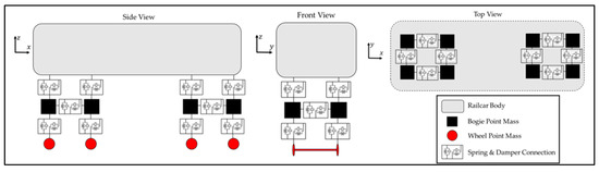
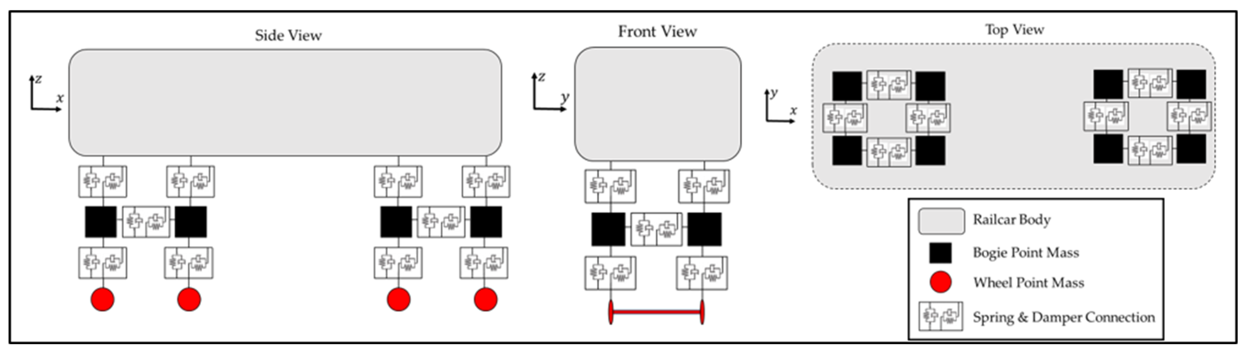
A 54-Degree-of-Freedom (DOF) three-dimensional lumped parameter model is used to represent each individual rail vehicle in the train consist. This model adequately captures both vehicle response and the impact of vehicle behavior on the train–track interaction effects. The model, depicted in Figure 1, consists of a massive rigid car body, two massive bogies, and four wheelsets connected through the primary and secondary suspension systems.
Figure 1.
54-DOF vehicle model schematic.
The car body is assigned six DOFs defined at its center of gravity, i.e., the vertical, longitudinal, lateral, pitching, rolling, and yawing DOFs notated . The front bogie comprises four rigid massive bodies connected by very stiff spring elements, as shown in Figure 1. The motion of each of the four bogie bodies is described by three translational DOF, i.e., the vertical, longitudinal, and lateral DOFs thus defining twelve bogie DOFs notated . The rear bogie is represented similarly to the front bogie with the corresponding DOFs notated . Eight wheels are assigned three translation DOFs representing the vertical, longitudinal, and lateral directions notated as: .
The primary suspension comprises spring–damper assemblies connecting the wheelsets to the bogies. The secondary suspension system also comprises spring–damper assemblies connecting the bogies to the car body. Two vehicle model variants are used for this study with parameter values selected from available data representing the equivalent of DOTX 117 and DOTX 220 vehicles. These values are listed in Table 1.
Table 1.
54-DOF vehicle model parameter values.
2.2. Vehicle-to-Vehicle Coupling
A critical component of analyzing the complexities of train behavior is the accurate modeling of the interaction between consecutive cars. In this study, a train is represented as a sequence of linked cars, with adjacent car bodies connected through spring–damper elements acting in the longitudinal, vertical, and transverse directions. A stiffness coefficient of 1595 kN/m and a damping coefficient of 80 kN·s/m are assigned to these coupling elements in each direction, thereby accounting for the transmission of forces and vibrations between consecutive railcars. This approach ensures a realistic representation of the dynamic coupling between each pair of consecutive cars and allows for the examination of the collective behavior of the entire train. The car-to-car couplers provide the structural continuity required to represent the train as an interconnected dynamic system. This integrated modeling strategy becomes particularly important in scenarios where the interaction between cars plays a crucial role, such as during acceleration, deceleration, or when traversing variable track conditions.
2.3. Track Model
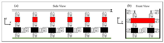
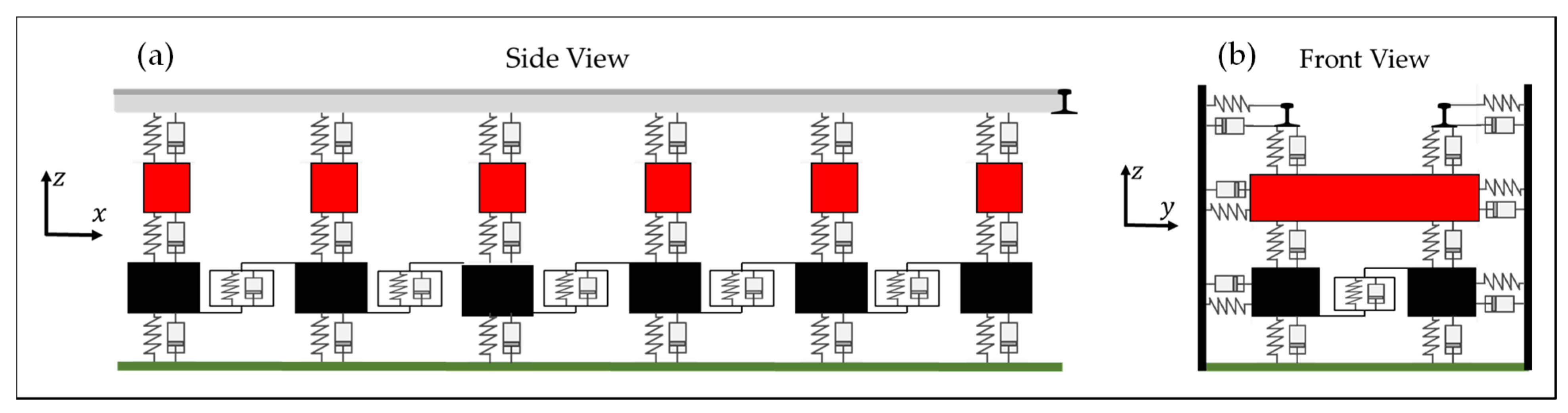
The 3D track structure is modeled in adequate detail to account for the rails, rail pads, sleepers, ballast, and subgrade individually. This ensures that the effects of each component can be modified separately and properly incorporated into the simulation. Figure 2 displays a schematic of the 3D track structure with selected track parameters listed in Table 2 [32].
Figure 2.
3D track (a) side view, (b) front view. Ties are shown in red and ballast in black.
Table 2.
Track parameters [32].
Rail segments are modeled as 2-node Euler–Bernoulli beams defined by two translational (vertical and lateral) and one rotational (pitching motion about the lateral direction) DOFs at each node. The Euler–Bernoulli rail elements are supported by a discrete layered foundation rather than a continuous Winkler-type foundation [33]. The support system is represented explicitly through rail-pad spring–damper elements, rigid sleepers, and lumped ballast and subgrade mass-spring–damper components [34]. Utilizing these DOFs enhances computational efficiency without compromising essential characteristics. Sleepers are modeled as rigid bodies equally spaced along the track whose motion is defined by three DOFs, i.e., vertical translation, rotation about the longitudinal track axis, and lateral translation. Spring–damper elements are used to represent the rail pads, between the rail and sleeper elements. The ballast and subgrade are represented as a lumped parameter model by interconnected mass, spring, and damper elements.
3. R-VTI Framework
The R-VTI framework employs a novel subsystem coupling technique called PDC. Unlike conventional monolithic methods, the proposed approach solves each subsystem (vehicle and track) independently and subsequently couples them iteratively, substantially reducing computational demands without sacrificing accuracy. This section outlines the fundamental components of the PDC technique, including subsystem solvers, global coordinate considerations, and the iterative coupling mechanism.
3.1. Subsystem Solver
A key feature of the proposed PDC technique is that the vehicle and track are treated as independent dynamic subsystems. Therefore, each subsystem can retain its own mathematical representation and numerical time-integration scheme. For each subsystem, the governing equation of motion is expressed as
where M is the mass matrix, C is the damping matrix, K is the stiffness matrix, is the displacement, is the velocity, is the acceleration, and is the external force vector. For the vehicle subsystem, the response vector contains the car-body, bogie, and wheelset DOFs defined in Section 2.1. Accordingly, the vehicle’s mass matrix is assembled from the corresponding masses and mass moments of inertia, while the damping and stiffness matrices are assembled from the primary and secondary suspension systems and the vehicle-to-vehicle couplers described in Section 2.1 and Section 2.2. For the track subsystem, the matrices are assembled from the rail, fastener, sleeper, ballast, and subgrade components described in Section 2.3. The corresponding force vectors include the external loads and wheel–rail interaction forces acting on each subsystem. Within each PDC iteration, Equation (1) is solved independently for the track and vehicle subsystems over the analysis interval. The track solver first determines the track response under the applied wheel loads. This response is transferred to the vehicle solver through the wheel–rail interface, where the vehicle response and updated wheel–rail forces are calculated. The resulting force histories are subsequently returned to the track subsystem for the next PDC iteration. This process continues until the convergence criterion described in Section 3.2.2 is satisfied. Thus, the subsystem solver provides the independent dynamic solutions, while the PDC procedure governs the exchange and convergence of the interaction quantities between the vehicle and track.
The PDC formulation is independent of the selected time-integration method. In this study, the Newmark-β, method [35] is employed for both subsystem solutions. The displacement and velocity updates are expressed as
where Δt is the time step, t + Δt denotes the next time step, and β = 1/4, and γ = 1/2 are the Newmark-β constants.
Rearranging Equation (2), the acceleration at the next step is obtained as
3.2. Subsystem Coupling via PDC Technique
3.2.1. Global Coordinate System
The global coordinate system in the PDC technique is essential for simulating the dynamic interaction between train and track subsystems. In this method, the coordinate system is fixed to the train, with the track moving beneath it to simulate train travel, an approach referred to as the “Treadmill Effect”. This strategy improves computational efficiency by truncating the track to a length that only needs to accommodate the train and its interaction with the track, excluding unaffected sections. Boundary conditions at the front and rear of the track domain are updated dynamically as the train advances, ensuring continuity of interaction forces. This approach ensures that the model remains computationally feasible even for long track lengths or complex railway networks by focusing on the areas actively interacting with the train, thereby reducing the overall computational load. This enables faster simulations and broader applications, such as real-time derailment potential assessments and system optimizations, all while achieving a balance between numerical efficiency and dynamic fidelity.
3.2.2. Train–Track Coupling
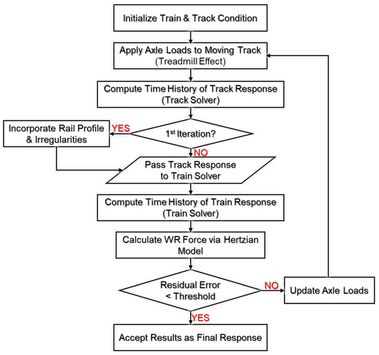
The R-VTI framework is designed to address the complex interactions between the train and track subsystems, enabling rapid analysis of derailment failure. The critical component of the framework is the train–track coupling via the PDC technique, which operates through an iterative analysis process focusing on one subsystem (either the train or the track) during each iteration and assessing its response to the actions of the other subsystem. As shown in Figure 3, the coupling process begins by defining the initial conditions of both train and track subsystems, which are set to zero. This step is followed by the application of axle loads to the moving track, in line with the Treadmill Effect. While computing the track response, the rail profile is incorporated into the rail movement in the first iteration. It is then passed through the train solver where utilizing the Hertzian contact model for wheel–rail (WR) forces as presented in [4], the track response is applied as excitation at the wheels of the train. In the present implementation, the rail profiles represent the longitudinal rail-surface and track irregularity input rather than the transverse rail-head geometry. The wheel is represented by its nominal rolling radius, (ro), with the corresponding values provided in Table 1. The wheel–rail interaction force is calculated using the nonlinear Hertzian contact formulation described in [4]. The instantaneous contact deformation is determined from the relative displacement between the wheel and rail at the contact location, including the rail dynamic response and the imposed rail irregularity. This contact deformation is subsequently used to calculate the nonlinear wheel–rail interaction force. Accordingly, the present model does not explicitly perform transverse wheel-profile and rail-head-profile matching; instead, the wheel geometry is represented through its nominal radius and the measured longitudinal rail profile is introduced as excitation at the wheel–rail interface. After completing track analysis using the Treadmill Effect for the entire length of the track, the new response of the train subsystem is calculated, accounting for both the track response and irregularities. This time history represents the dynamic performance of the train in response to track conditions.
Figure 3.
Pseudo-dynamic coupling flowchart.
In the subsequent iteration, dynamic loads resulting from the train interacting with the track are used in place of axle loads for the track analysis. The same approach is applied to both subsystems, with the key difference being the inclusion of rail roughness in the track model. The train and track are analyzed in parallel, and new time histories are generated for both subsystems. The difference between this iteration and the previous one reflects the changes in track performance caused by the dynamic loads exerted by the train, accounting for the updated interaction between the two systems. At this point, the time histories from the current iteration are compared with those from the previous iteration to calculate the residual error. If the residual is smaller than a predefined threshold, such as that specified in [4], the time histories are accepted as the final response of the system. If the residual exceeds the threshold, the iteration process continues, and the system undergoes another round of analysis with updated inputs. This iterative process repeats until the residual reaches an acceptable level, ensuring that both subsystems converge to a stable solution. Once convergence is achieved, the final dynamic behavior of the entire train–track system is obtained. The main distinction of the PDC technique is that the vehicle and track are solved as independent subsystems over the complete analysis interval, with response and wheel–rail force histories exchanged through an outer coupling iteration rather than within each individual time step. This separation allows different subsystem solvers and, together with the Treadmill Effect, reduces computational effort while retaining the dynamic interaction between the vehicle and track.
3.3. Derailment Criteria
Although there are a variety of criteria for predicting train derailments [36,37,38,39,40], this study implements two of the most common: the L/V ratio and vertical force reduction. The L/V ratio is particularly useful for identifying flange-climb derailments, while vertical force reduction highlights unloading risks on degraded track.
The derailment coefficient, defined as the ratio of lateral (L) to vertical (V) load at the wheel–rail contact point, is widely used and commonly referred to, as in this work, as the L/V ratio. The L/V ratio is a relatively conservative quantification of derailment failure and it is used in this study because of its widespread acceptance, and is defined as [22]:
where T is the tangential force across the flange, N is the normal force on the flange, and α is the flange angle at the wheel–rail contact point. Generally accepted limiting values of L/V vary across regions: the British Standard [41] states that L/V must not exceed 1.2; the Japanese standard states L/V must not exceed 0.8 for more than 50 milliseconds [36]; in China, L/V should not exceed 1.0 [22]; and in North America, L/V should not exceed 1.5 [40]. A threshold value of L/V less than 1.5 is adopted for this study.
The second derailment criterion considered in this study is the reduction in the wheel normal force, typically expressed as [22]:
where is the reduction in dynamic wheel load compared to the static wheel load, . Standards vary in their acceptable limits for vertical force reduction. The British Standard [42] recommends ΔQ/Q0 less than 0.6, while North American guidelines permit reduction up to 0.9 [40]. A threshold value of 0.9 is adopted for this study.
4. PDC Technique Verification
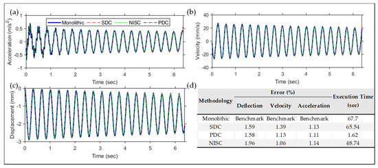
The train and track models developed in this study are used to verify the accuracy and efficiency of the proposed PDC technique through comparison with other established methodologies: (i) Non-Iterative Substructure Coupling (NISC), (ii) Staggered Dynamic Coupling (SDC), and (iii) the conventional monolithic approach utilizing the general-purpose finite element software Abaqus, with the monolithic method serving as the benchmark for validation. The verification model has a vehicle length of 21 m traversing a 192-meter-long track at a speed of 96.5 km/h (60 mph). The execution time was recorded for each case and normalized with respect to the execution time of the benchmark. The percent error with respect to the benchmark solution is calculated using Equation (7). Figure 4 illustrates the comparative performance of the methodologies.
Figure 4.
Comparison of subsystem coupling techniques for train–track interaction for vehicle (a) acceleration, (b) velocity, and (c) displacement with (d) percent error and execution time.
The PDC technique not only maintained a competitive accuracy level but also exhibited remarkable efficiency with the execution time reduced to 2.4% of that of the monolithic approach. This substantial reduction in execution time emphasizes the efficiency of the PDC technique. Additionally, PDC demonstrates a better trade-off between accuracy and execution time, highlighting its effectiveness for analyzing the dynamics of longs traversing over tracks and conducting derailment safety assessments, as utilized in this paper. The computational advantage of PDC results primarily from the separation of the vehicle and track into independently solved subsystems. In the monolithic approach, all vehicle and track DOFs are assembled into a single global system and solved simultaneously during time integration. PDC instead solves the smaller subsystem equations independently and exchanges only the required wheel–rail force and response histories through the coupling iterations. Furthermore, the Treadmill Effect restricts the modeled track to the active interaction domain. Consequently, PDC avoids repeated solutions of the larger globally coupled system, which accounts for the substantial reduction in wall-clock computation time observed in Figure 4.
5. Model Validation via Field Measurements
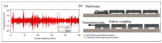
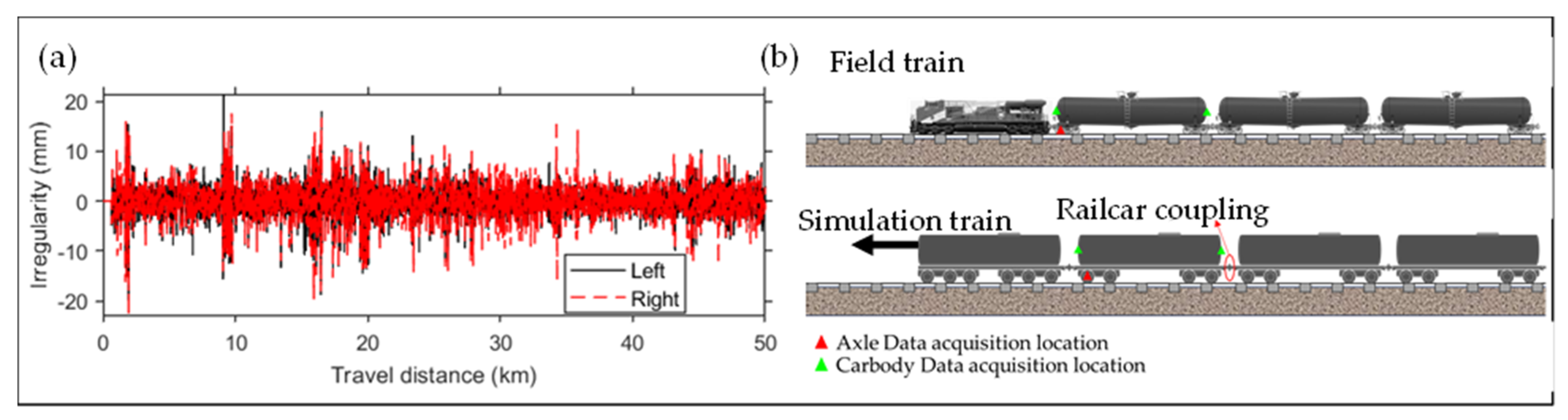
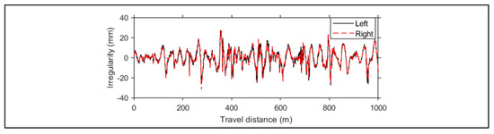
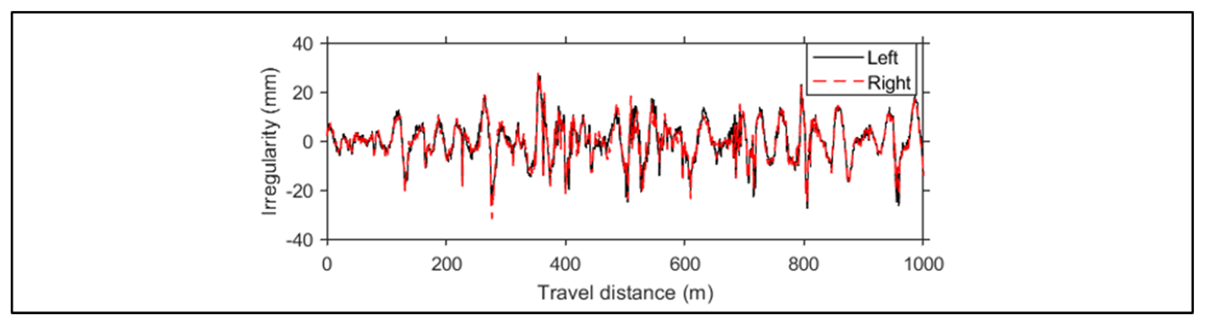
Following the numerical verification of the PDC technique in Section 4, this section evaluates the physical validity of the complete R-VTI framework through comparison with field measurements. The numerical comparison in Section 4 and the field comparison presented here serve complementary purposes. The monolithic solution provides a benchmark for verifying the numerical accuracy of the PDC technique, whereas agreement between two numerical models does not by itself establish their physical fidelity because they may share common modeling assumptions and parameter uncertainties. The field measurements therefore provide an independent validation of the complete R-VTI framework, including the vehicle, track, and wheel–rail interaction representations, against actual train–track response. Vibration response data from an instrumented test train (referred to as ‘field train’) were provided by the FRA. The field train consists of an AAR 112 diesel locomotive and three DOTX 117 tank cars. The first tank car was equipped with vibration sensors mounted on both the left and right sides of the first axle, and on the front and back ends of the car body during the field test. The field train acquired vibration data along approximately 100 km of track for which the left and right rail profiles had been obtained by a track-geometry vehicle. The recorded rail profiles were directly used as input to the track model to ensure realistic excitation conditions. The rail profiles and the field and test train configurations are shown in Figure 5.
Figure 5.
(a) Provided left and right rail profiles and (b) schematics of field and simulation trains.
The train model used for the simulation (referred to as ‘simulation train’) was configured to be consistent with the field train, and the cars are interconnected using the presented vehicle-to-vehicle coupler scheme. To maintain the actual speed from the field, a controlling tractive force is applied to the simulation train and is adjusted at every time step of the solution to maintain the actual field train’s speed. As in the field train, the first axle and the two ends of the car body of the first tank car are monitored for the validation study.
The recorded vibration measurements were truncated to a length of two kilometers, when the train was traveling at a constant speed of 88.5 km/h (55 mph). The exact location where this 2 km long section of track lies along the provided rail profile was unknown because the data were not synchronized. To resolve the uncertainty of the location of the vibration measurements, a moving-window correlation method was applied, in which the shorter field signal is shifted over the full simulated data to identify the segment of maximum correlation. Once the approximate location was determined, simulation results corresponding to that track segment were extracted and used for comparison with the field data.
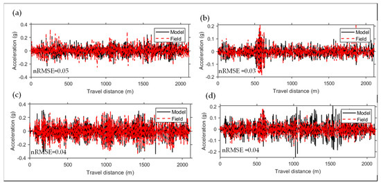
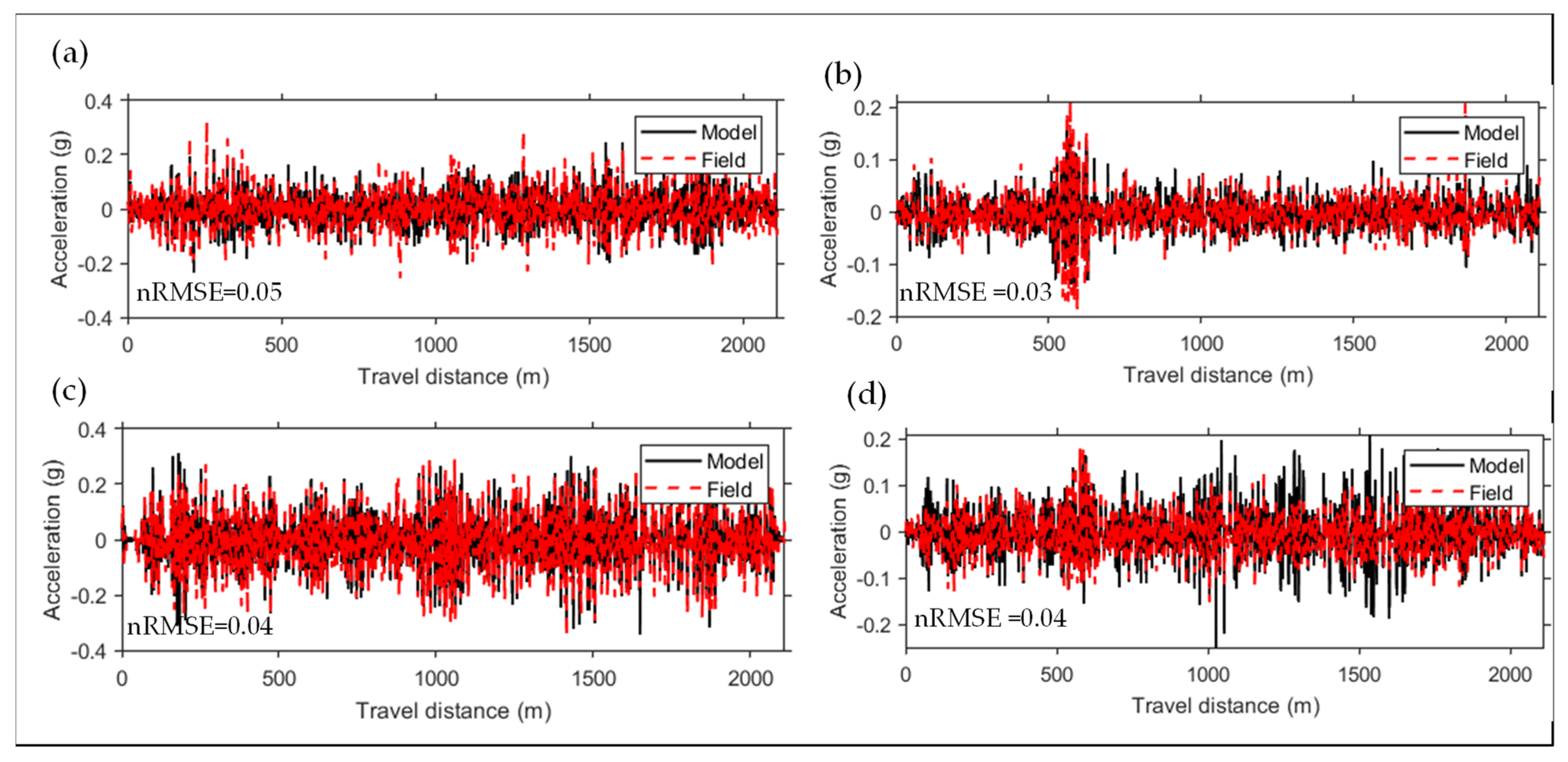
Figure 6 displays the comparison of vertical and lateral car body accelerations at the front and back end of the first car. Comparing the results shows that the simulation responses are in general agreement with the field data, especially considering the uncertainties regarding the actual location of the vibration measurements, and the different times at which the geometry and vibration measurements were acquired. The agreement was quantified using the normalized Root Mean Square Error (nRMSE), defined as
where n is the length of signals. All nRMSE values are less than 0.05, indicating that the model error remains below 5% of the measured signal range and the model captures the main dynamic response within acceptable accuracy.
Figure 6.
Comparison of field vs simulation 1st car-body results for (a) front-end vertical accelerations, (b) front-end lateral accelerations, (c) back-end vertical accelerations, and (d) back-end lateral accelerations.
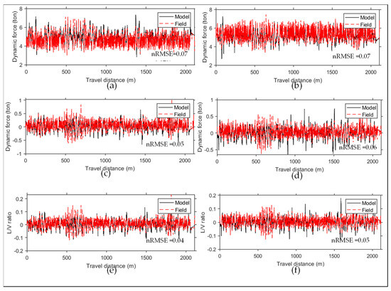
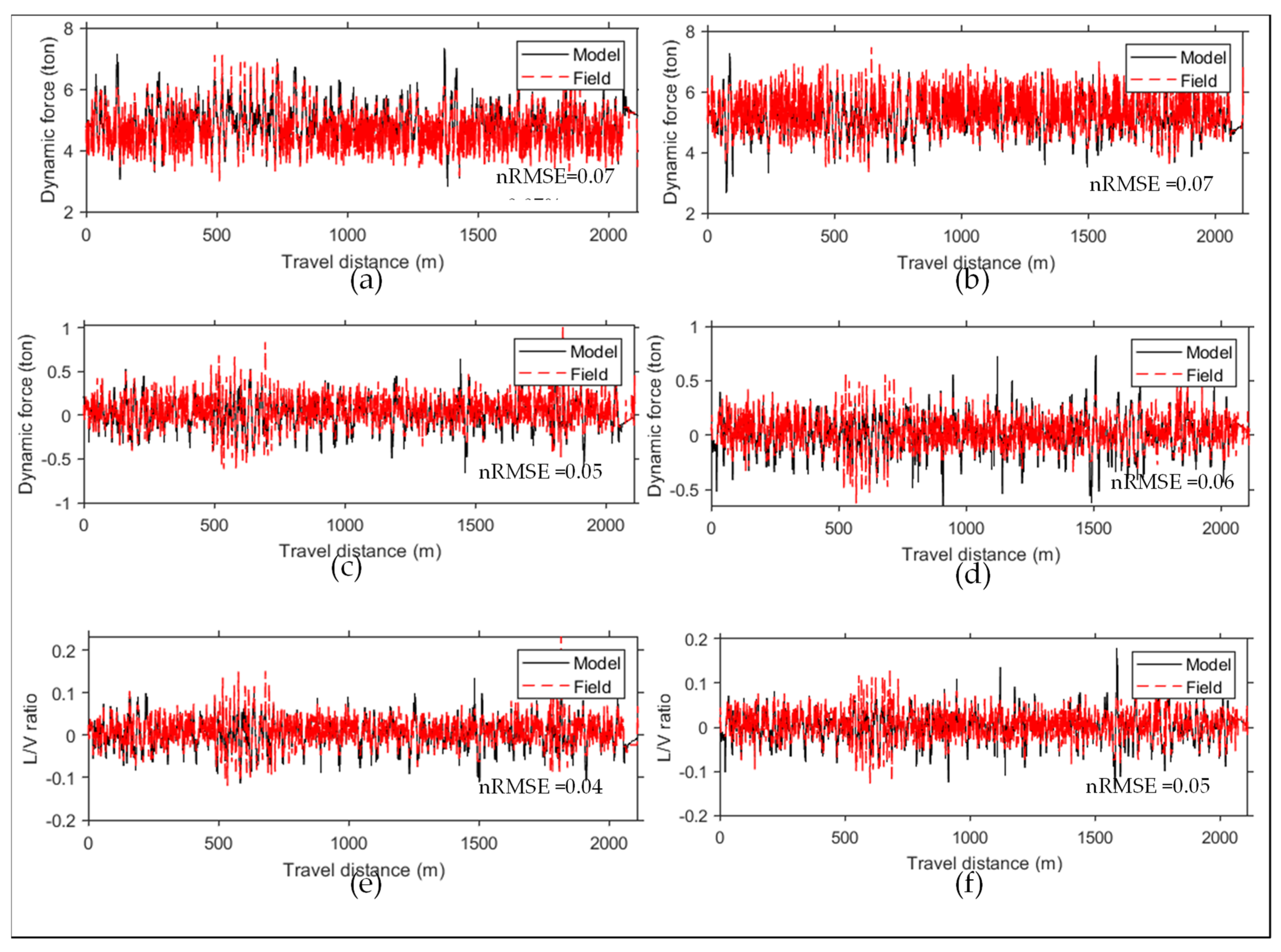
Next, the vertical and lateral components of the wheel–rail contact force at the left and right sides of the equipped axle of the field and simulation trains are compared, and plotted in Figure 7a,b. The DOTX 117 vehicle has a light weight of approximately 41,300 kg [43], corresponding to a nominal static load of about 5.16 t per wheel when distributed over its eight wheels. This value is consistent with the quasi-static vertical wheel–rail force level observed in Figure 7. The simulated results are in general agreement with the field measurements, particularly considering the uncertainties and noise in the measurements. It is observed that the vibration characteristics (shape and amplitude) of the contact forces are in good agreement. This study specifically evaluated the L/V ratio using the proposed nonlinear Hertzian contact model. As illustrated in Figure 7e,f, the L/V ratios derived from the simulation were in close correspondence with the measured ratios, with nRMSE values below 5%. These results confirm that the R-VTI framework is capable of predicting both the absolute contact forces and their relative magnitudes within acceptable accuracy.
Figure 7.
Comparison of field vs simulation axle results for measurements of (a) left and (b) right wheel–rail vertical dynamic force, (c) left and (d) right wheel–rail lateral dynamic force and calculated (e) left and (f) right L/V ratios.
6. Implementation Example: Assessment of Derailment Potential
This section presents an implementation case study of the proposed R-VTI framework on one of the common failures in railway: derailment. Real-world track measurements are used with multiple train loading configurations to determine the level of risk as defined by typical derailment criteria. This allows train configurations with higher-than-acceptable risk levels to be identified and appropriately addressed to mitigate the risk.
6.1. Track Measurements
Field data consisting of the track profile, shown in Figure 8, were recorded via DOTX 220 for a segment of the Precision Test Track (PTT) at the Technology Testing Center (TTC) and provided by the FRA.
Figure 8.
DOTX220 recorded track profile.
6.2. Combined Effects of Train Configurations and Track Condition
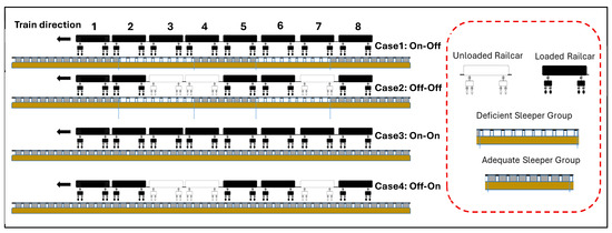
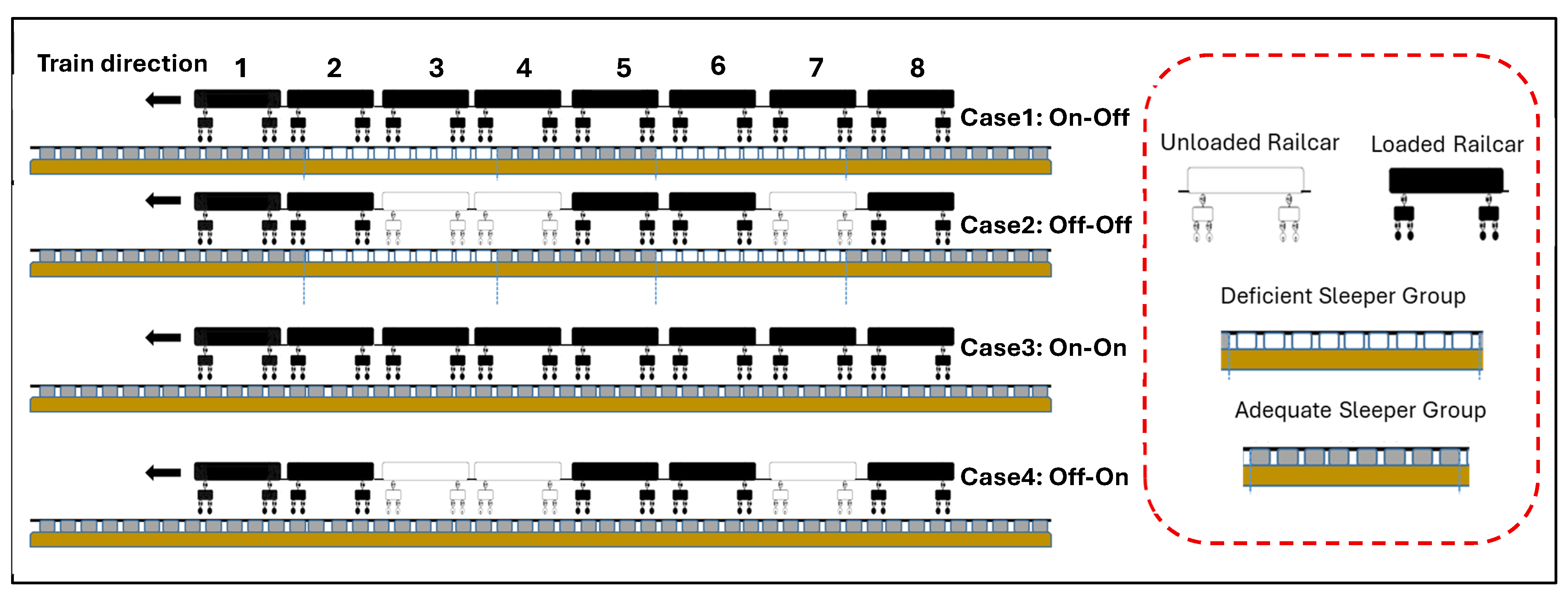
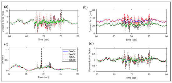
This section investigates the combined effects of train configuration and track condition on derailment failure using the R-VTI framework. The first part of this study considers a tangent track traversed at a speed of 96.6 km/h (60 mph) by a train consisting of eight 54-DOF cars (one locomotive and seven tank cars). Two train configurations are considered: (i) where all cars are fully loaded (119,295 kg) and (ii) a mixed-load configuration in which the second, third, and seventh cars are unloaded (88,450 kg). Two track configurations are considered: (i) a fully intact track and (ii) a track containing several deficient sections represented by removing groups of nine consecutive sleepers. To simplify the nomenclature, intact track segments are denoted as ‘On’, while track segments with missing sleepers (i.e., deficient track) are denoted as ‘Off’. The same-name convention is also used for the train configuration in this example: if the cars are fully loaded, it is identified as ‘On’, and ‘Off’ refers to the mixed-load case. Each case of train–track combination is then named based on these designations, such as ‘On-Off’ where the first term characterizes the train configuration, and the second term indicates the track configuration. Therefore, ‘On-Off’ pertains to a fully loaded train over a track with missing sleepers. Figure 9 illustrates the schematics of the selected cases.
Figure 9.
Initial train–track configurations for simulation.
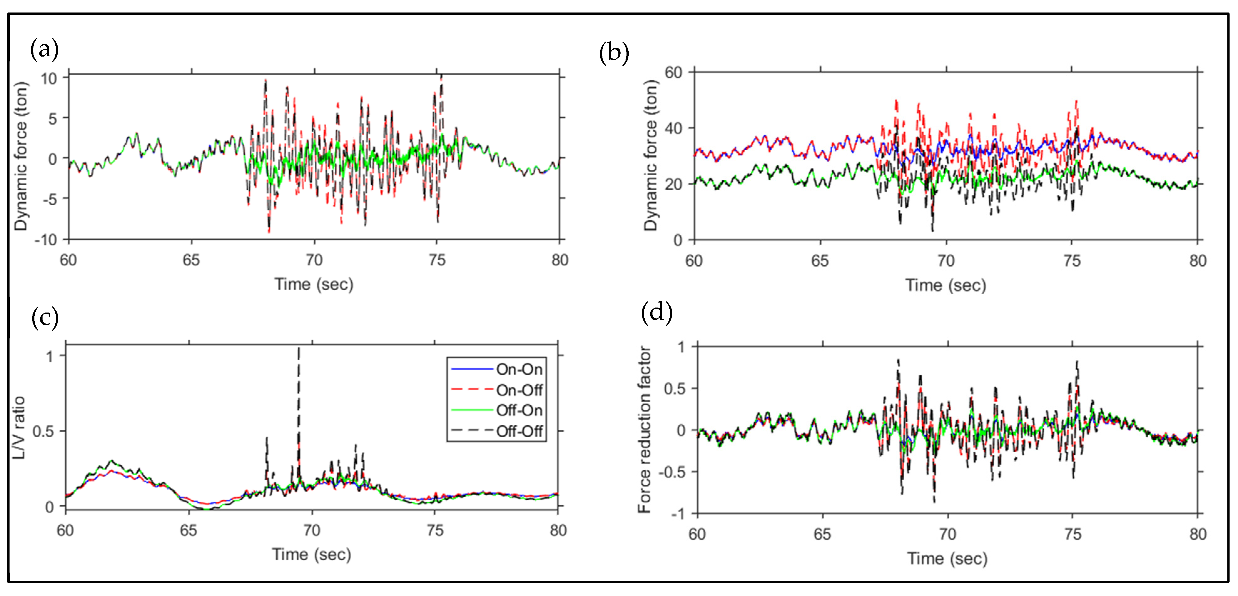
The derailment risk is quantified for all axles using both the L/V ratio and force reduction criteria. A notable finding emerges, indicating that the ninth axle of the train consistently experiences more than 50% variation in vertical interaction across all examined cases. Simultaneously, the lateral load undergoes substantial fluctuations within this specific track segment. This makes the ninth axle an ideal representative for illustrating the combined effects of car loading and sleeper deficiency, as it captures the compounding impact of both variables at a mechanically vulnerable location in the consist. The dynamic loads on this critical ninth axle are shown in Figure 10a,b, and the resulting derailment criteria are shown in Figure 10c,d, demonstrating the significant influence exerted by track health status on the overall performance of the train. The effect of the deficient track segments on the vehicle response is clearly identified between 67 and 76 s, with significant fluctuation in the dynamic loads. Analysis of the L/V ratios indicates a critical moment around 70 s where the ratio for the Off-Off configuration surpasses 1.1 and the On-Off configuration surpasses 0.45. While these values do not exceed the adopted threshold value of 1.5, they indicate a higher risk of derailment relative to the rest of the simulation. These transient spikes are not present in the two configurations which do not contain track deficiencies, indicating the ability of the simulation to detect regions of track deficiencies quite effectively. Further, the highest ratio corresponds to a scenario with an unloaded car and deficient track, which quantifies conventional wisdom.
Figure 10.
Ninth axle (a) lateral and (b) vertical dynamic loads and calculated (c) L/V ratio and (d) force reduction.
A parallel analysis of the force reduction derailment criteria similarly identifies the unloaded car and deficient track configuration as the most critical. In this instance, the vertical force reduction exceeds that of other cases, reaching 80 percent. This substantial reduction approaches the threshold value of 90 percent and results in a greater potential for wheel lift, especially under poor track conditions. These comprehensive evaluations reveal the complex interactions between track integrity, loading conditions, and derailment failure, and demonstrate how the R-VTI framework provides quantitative insights for enhancing railway safety and operational resilience.
6.3. Axle-Level Derailment-Failure Distribution
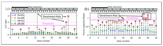
The L/V ratio, the key measure in assessing derailment susceptibility, clearly indicates that unloaded cars exhibit greater potential for derailment. Figure 11 shows the maximum derailment criteria values calculated for each axle across all configurations. In Figure 11a, the magenta dashed line marks the L/V derailment threshold of 1.5, above which derailment becomes more likely. Notably, the Off-Off configuration (dark markers) exhibits multiple L/V spikes above this threshold, particularly Axles 13, 27, and 28. Mapping axle positions to the train configuration shown in Figure 9, these axles correspond to unloaded Railcars 4 and 7, respectively, and their elevated L/V ratios reflect a combination of minimal downward force (due to unloading) and increased lateral disturbance (from deficient track). The fact that Axle 13 is the leading axle of an unloaded car preceding another unloaded railcar further amplifies transient vibration effects, leading to lateral destabilization. This pattern indicates that unloaded railcars traveling over deficient track sections significantly amplify lateral forces, raising derailment concerns. The On-Off configuration (red markers) also shows elevated L/V ratios, though to a lesser extent, underscoring that even when the train is loaded, riding over damaged track poses localized derailment potential. Meanwhile, the Off-On and On-On configurations (green and blue markers) remain consistently below the critical threshold, emphasizing that intact track conditions can mitigate risk.
Figure 11.
Derailment criteria for each axle of each train configuration: (a) L/V ratio and (b) force reduction.
In Figure 11b, the threshold value is set at 0.9, beyond which a significant loss of vertical force indicates a high likelihood of wheel unloading or lift-off. The Off-Off configuration (black markers) clearly dominates in terms of criticality, with multiple axles, including Axles 16, 26, 27, and 28, exceeding the threshold. Mapping these axles to their corresponding railcars, Axle 16 belongs to the unloaded Railcar 4, while Axles 26 to 28 are associated with Railcar 7, which is also unloaded. The severe force reduction in these axles results from a synergistic effect of low static load due to unloaded cars and dynamic disturbance from underlying deficient track segments. In particular, Railcar 4 lies in between unloaded and loaded railcars, reducing its inertia and amplifying its response to vertical irregularities. Notably, in the On-Off configuration (red markers), Axles 26 and 28 also surpass the threshold, revealing that even a fully loaded train is susceptible to derailment failure if critical railcars travel over structurally compromised track segments. The Off-On and On-On configurations (green and blue markers, respectively) show consistent vertical forces well below the critical threshold across all axles, reaffirming the stabilizing effect of full loading or intact track.
Comparing these two criteria, while both the L/V ratio and force reduction plots highlight critical derailment risks, the force reduction criterion appears more sensitive, identifying a broader range of at-risk axles. In contrast, the L/V ratio isolates fewer but more severe spikes, suggesting it captures acute derailment events, whereas force reduction reflects overall loss of stability. These observations confirm that derailment failure escalates not only with localized deficiencies and unloading but also due to car sequence and spatial positioning.
6.4. The Effect of Different Train Configurations
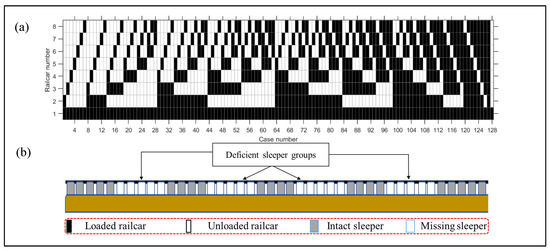
The efficiency of the presented R-VTI framework allows many varied conditions to be run quite quickly, giving a more complete understanding of whether the train or the track is the source of the elevated derailment potential. As an example of this, a parametric study was conducted involving the eight-car train running over the profile shown in Figure 8. In this study, 128 unique combinations of loaded and unloaded cars were analyzed. To investigate the impact of railcar-loading patterns on potential derailment failure, all 128 train loading scenarios were visualized using a binary-loading matrix shown in Figure 12a. In the loading matrix, each configuration (columns) shows which of the eight railcars (rows) are loaded (black) or unloaded (white). The locomotive (first car) remains loaded in all cases. Configurations range from lightly loaded trains at the beginning to fully loaded ones toward the end. The last configuration in the matrix represents a train with all trailing railcars unloaded. Notably, the sequence includes various patterns such as front-heavy, rear-heavy, alternating, and clustered loading combinations. In this study, a loaded–unloaded transition is defined as the interface between two consecutive railcars having different loading states, i.e., a loaded car followed by an unloaded car or an unloaded car followed by a loaded car. These interfaces create local mass discontinuities along the consist and can increase the dynamic response of nearby axles. The track is represented in a damaged state, with four sections of five consecutive missing sleepers, separated by four healthy sleepers. The spatial layout of these deficient segments is shown in Figure 12b.
Figure 12.
(a) Binary loading matrix of 128 different train configurations and (b) schematic of track condition used.
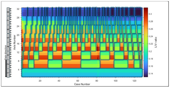
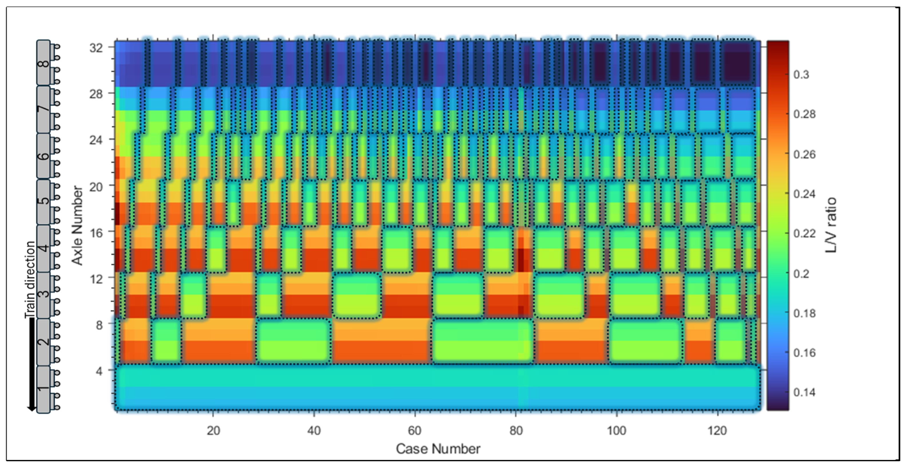
Figure 13 presents a heatmap of the L/V ratio variation across all 128 train loading configurations for all axles. Here, the dashed boxes indicate which railcars are loaded in each case, progressing systematically from one loaded trailer at the front of the train to all cars loaded toward the far right. Among all scenarios, Cases 1, 81, and 82 show the highest L/V ratios exceeding 0.30. These cases involve positioning unloaded railcars trailing behind the locomotive and around the mid-train. Such configurations likely create significant stiffness and mass discontinuities, which contribute to localized lateral force amplification and dynamic instability, particularly at the interface between loaded and unloaded segments. As shown in this heatmap, Case 1 includes only two loaded railcars at the front, followed by six unloaded ones. The critical axles identified in this scenario are Axles 13,14, 17, and 18, all of which fall within Railcar 4 and Railcar 5, specifically in their leading bogies. This is noteworthy because it shows that leading bogies are more affected rather than the rear bogies. These cars form a mid-train cluster of low mass, among other unloaded cars. The lack of vertical force on these axles reduces the normal force at the wheel–rail interface, making the wheels more susceptible to lateral instability and increased L/V ratios. Because the unloaded cars are being pulled by heavier loaded cars at the front, inertial effects and traction forces contribute to lateral instability in the first few unloaded cars. This results in the critical loading seen in the leading axles of Railcars 4 and 5. Notably, the rear-most unloaded cars (Railcars 6–8) are less critical, suggesting that leading axles of mid-train unloaded cars are more affected by dynamic forces from preceding loaded segments. In Cases 81 and 82, Railcars 3 and 4 are unloaded in both, with Railcar 7 unloaded in Case 81 and Railcar 6 in Case 82. Despite this small difference, Case 81 shows greater instability, as the two front unloaded railcars are in between loaded ones, intensifying dynamic transitions and elevating L/V ratios.
Figure 13.
Heatmap of L/V ratios for 128 train loading configurations (dashed boxes mark loaded cars).
By the time most cars are loaded (Cases ≈ 100–127), the heatmap turns predominantly cooler (green-blue), with L/V ratios reduced across nearly all axles. Case 127, with all cars loaded, exhibits low L/V values, while Case 128, where all trailing railcars are unloaded, shows considerably higher L/V ratios in warm tones, indicating elevated derailment potential due to reduced train stability. In Cases 120–123, relocating a single unloaded railcar from the rear toward the front leads to a noticeable increase in L/V ratios, suggesting that positioning light cars near the locomotive intensifies dynamic instability. This pattern is consistently observed in other groups, including Cases 99–105 (two unloaded cars) and Cases 64–67 (three unloaded cars), where rearward unloading yields lower risk. A similar pattern persists in other scenarios such as Cases 29 to 32 and Cases 8 and 9 for four and five unloaded railcars, respectively. The L/V ratio heatmap shows that, for an equal number of unloaded railcars, scenarios with unloaded cars placed closer to the locomotive or mid-train produce greater instability.
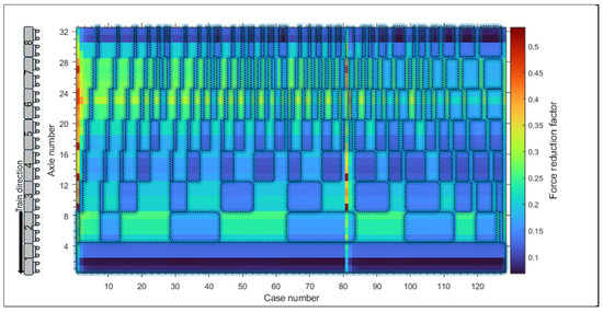
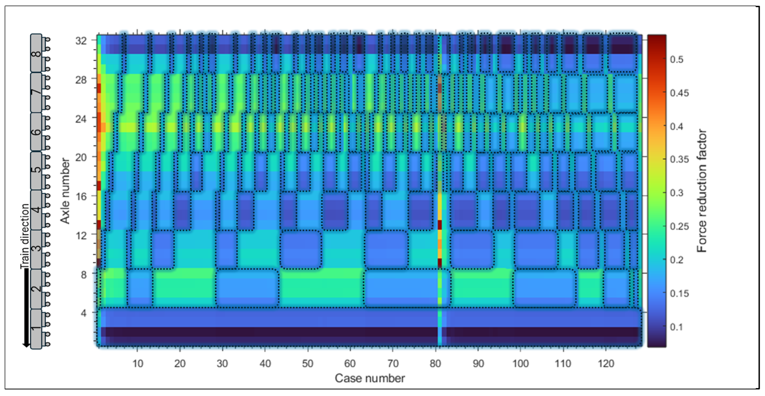
Figure 14 presents the heatmap of vertical force reduction across all 128 train loading configurations, and dashed boxes indicate the loaded cars. Similar to the L/V analysis, the highest vertical force reduction is observed in Cases 1, 81, and 82. In Case 1, the most critical axles are located in Railcars 3 and 4 that experience a reduction exceeding 0.50, indicating substantial loss in normal load. These railcars form an unloaded cluster in the mid-train region, exacerbated by abrupt mass transitions from the loaded front segment. In Case 81, Railcars 3, 4, and 7 are unloaded. The highest reduction is again concentrated around the leading axles of Railcars 3 and 4, driven by their adjacency to mass discontinuities and compounded by dynamic forces from preceding loaded cars. In contrast, although Case 82 has a similar setup, with Railcars 3, 4, and 6 unloaded, the reduction is lower. This difference arises from the position of the third unloaded car: shifting it from Railcar 7 to 6 in Case 82 alleviates the severity of vertical force reduction in the mid-train region, though the risk remains elevated.
Figure 14.
Heatmap of vertical force reduction for 128 train loading configurations (dashed boxes mark loaded cars).
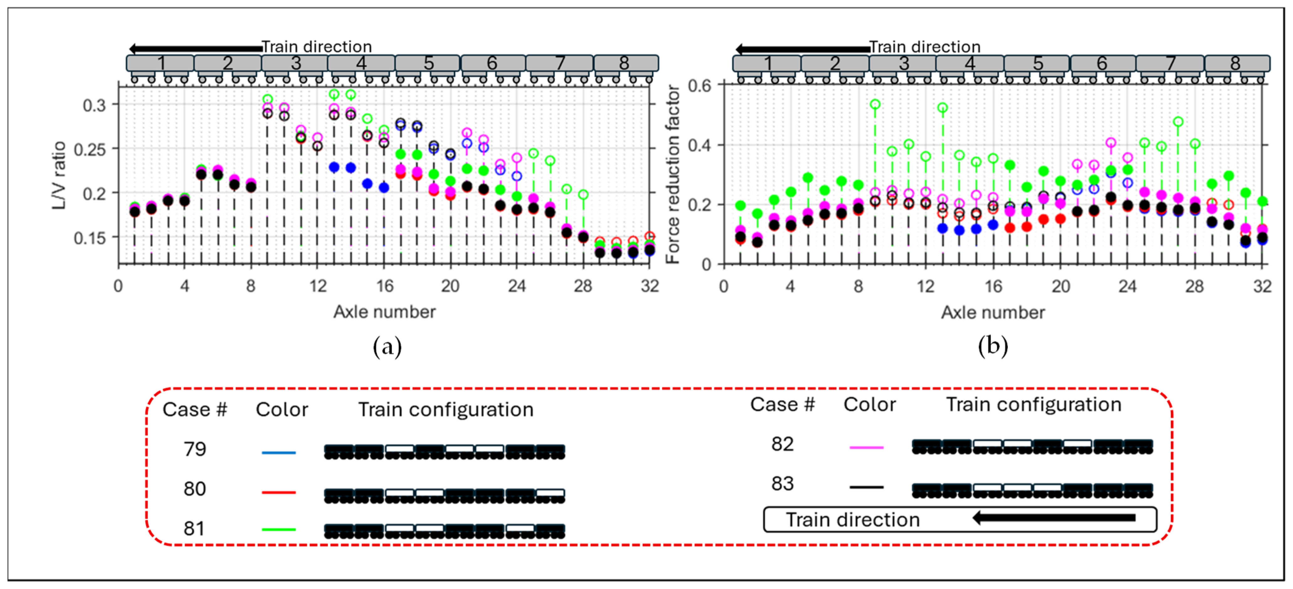
6.5. Case Comparison
Figure 15 illustrates the calculated derailment criteria for five selected cases using two complementary metrics: (a) L/V ratio and (b) force reduction factor, plotted across all train axles. Filled circles represent axles in loaded railcars, while open circles denote those in unloaded railcars. The results highlight distinct jumps in both criteria, particularly at locations where loaded and unloaded cars are coupled, indicating the dynamic effects of abrupt load transitions. This is corroborated by additional observations of Figure 13 and Figure 14, wherein it can be seen that the critical axles consistently align with unloaded cars. This demonstrates the greater stability of loaded cars. Further analysis shows that the first axle of a railcar tends to be more critical than the other axles on the car. This highlights their greater exposure to abrupt dynamic forces (e.g., tractive effort, lateral steering input). Interestingly, across all the train configurations studied, in no case were the four critical axles located on the locomotive, the first car, or the last car even if it is unloaded. This suggests that derailment failure tends to concentrate in the front and intermediate sections of the train, particularly among partially or fully unloaded cars near dynamically sensitive regions. This supports the hypothesis that mass in the front half of the train has a greater stabilizing influence on dynamic forces.
Figure 15.
Calculated (a) L/V ratio and (b) force reduction derailment criterion for each axle of selected cases.
In Figure 15a, the highest L/V ratios are consistently found in the leading bogies of unloaded railcars, especially when these cars are placed in the front or center of the train. In Figure 15b, however, for some cases such as Case 82, the highest values could occur in the rear bogies. Additionally, a clear declining trend is observed in the L/V ratio from mid-train onward. This supports the notion that placing unloaded cars toward the rear helps contain instability within a limited range of axles. Moreover, axles within the same railcar respond differently depending on whether adjacent cars are loaded. For instance, the values of both criteria at Axle 13 in Case 81 are higher than in other cases, even though Axle 13 belongs to the same car across all cases. This demonstrates that axle behavior is not solely a function of its own load status but is highly influenced by adjacent car conditions. Another notable pattern in this figure is the direct effect of railcar loading on derailment failure. For the same railcar position across different cases, the values clearly decrease when that railcar is loaded rather than unloaded. For instance, Railcar 4 shows critical values in all configurations where it is unloaded, but in Case 79, where it is loaded, the corresponding axle values drop significantly. This illustrates how increasing the vertical load on a railcar enhances its wheel–rail interface stability. It also highlights the nonlinear sensitivity of derailment failure to changes in load distribution: small shifts in which railcars are unloaded can cause localized spikes in lateral forces. These findings further emphasize that optimal loading strategies should prioritize distributing unloaded railcars toward the rear and avoiding clusters of unloaded cars in the front or mid-train.
7. Conclusions
The R-VTI framework introduced in this study demonstrates an efficient and scalable methodology for assessing derailment failure through the rapid evaluation of train–track configurations. By allowing the use of any numerical solver and subsystem coupling scheme, this framework significantly improves computational efficiency for large-scale analysis. At the core of the R-VTI framework is the PDC technique, which achieves accuracy comparable to monolithic solutions while reducing execution time to less than 3% of traditional methods. Validation against FRA field data confirmed the ability of the framework to capture vehicle and track dynamics with less than 5% error. The derailment failure assessment examples further demonstrate the framework’s capability to identify poor train–track configurations that fall outside of acceptable derailment criterion limits. Furthermore, the framework enables axle-specific and location-specific risk identification, making it possible to pinpoint the root causes of elevated derailment failure. By enabling efficient evaluation of large datasets, the R-VTI framework supports targeted risk mitigation strategies, such as optimized vehicle loading and prioritized maintenance scheduling. As a practical and computationally efficient tool, the R-VTI framework has the potential to advance current derailment failure assessment practices that contribute meaningfully to railway safety and operational resilience. Although the present study focuses on tangent-track applications, the R-VTI framework is not inherently restricted to tangent alignment. The same coupling strategy can be extended to curved track and turnout sections by incorporating the corresponding track geometry, wheel–rail contact kinematics, and lateral dynamic effects into the vehicle and track subsystem models. Validation of these applications remains part of future work. Overall, this paper shows that not only the number, but also the position of unloaded railcars is critical. Configurations where unloaded cars are clustered near the front or center exhibit higher L/V ratios, especially in their leading axles, highlighting the role of the dynamic force propagation and local mass discontinuities in derailment failure. These findings emphasize the operational importance of avoiding abrupt transitions between loaded and unloaded cars, particularly near the front or middle of the train. Optimal loading strategies should therefore avoid clustering unloaded cars in the front or mid-train and instead favor distributing them toward the rear.
Author Contributions
Conceptualization, D.C.R. and R.N.; methodology, D.C.R. and R.N.; software, R.N.; validation, R.N. and B.L.G.; formal analysis, R.N. and B.L.G.; writing—original draft preparation, R.N.; writing—review and editing, D.C.R. and B.L.G.; project administration, D.C.R.; funding acquisition, D.C.R. All authors have read and agreed to the published version of the manuscripts.
Funding
This work has been funded by the U.S. Department of Transportation Federal Railroad Administration under contract 693JJ620C000013. The opinions expressed in this article are solely those of the authors and do not represent the opinions of the funding agency.
Data Availability Statement
Data will be made available on request.
Acknowledgments
The authors have reviewed and edited the output and take full responsibility for the content of this publication.
Conflicts of Interest
The authors declare that they have no known competing financial interests or personal relationships that could have appeared to influence the work reported in this paper.
Abbreviations
The following abbreviations are used in this manuscript:
| R-VTI | Rapid Vehicle–Track Interaction |
| DOF | Degree of Freedom |
| nRMSE | Normalized Root Mean Squared Error |
| PDC | Pseudo-Dynamic Coupling |
| NISC | Non-Iterative Substructure Coupling |
| SDC | Staggered Dynamic Coupling |
References
- Islam, D.; Laparidou, K.; Burgess, A. What mitigation technique should be implemented to reduce freight vehicle derailments by 2050? In Proceedings of the Transport Research Arena (TRA) 2014, Paris, France, 14–17 April 2014. [Google Scholar]
- Federal Railroad Administration. Track Safety Standards Compliance Manual, Chapter 1: Introduction/General Guidance; Office of Safety Assurance and Compliance, Track and Structures Division, U.S. Department of Transportation: Washington, DC, USA, 2008.
- Gedney, B.L.; Naseri, R.; Al Kharousi, S.; Rizos, D.C. B-Spline signature responses in structural change detection: Method development. Struct. Health Monit. 2025, 24, 2911–2926. [Google Scholar] [CrossRef] [Scilit]
- Naseri, R.; Mohammadzadeh, S.; Rizos, D.C. Rail surface spot irregularity effects in vehicle-track interaction simulations of train-track-bridge interaction. J. Vib. Control 2025, 31, 738–752. [Google Scholar] [CrossRef] [Scilit]
- Tong, Y.; Liu, G.; Yousefian, K.; Jing, G. Track vertical stiffness—Value, measurement methods, effective parameters and challenges: A review. Transp. Geotech. 2022, 37, 100833. [Google Scholar] [CrossRef] [Scilit]
- Paixão, A.; Fortunato, E.; Calçada, R. A contribution for integrated analysis of railway track performance at transition zones and other discontinuities. Constr. Build. Mater. 2016, 111, 699–709. [Google Scholar] [CrossRef] [Scilit]
- Shi, C.; Zhou, Y.; Xu, L.; Zhang, X.; Guo, Y. A critical review on the vertical stiffness irregularity of railway ballasted track. Constr. Build. Mater. 2023, 400, 132715. [Google Scholar] [CrossRef] [Scilit]
- Jiang, Y.; Chi, M.; Yang, J.; Dai, L.; Xie, Y.; Guo, Z. Investigation on the mechanism and measures of derailment of empty freight train passing a turnout in the diverging route. Eng. Fail. Anal. 2024, 156, 107822. [Google Scholar] [CrossRef] [Scilit]
- Lai, J.; Wang, K.; Xu, J.; Wang, P.; Chen, R.; Wang, S.; Beer, M. A failure probability assessment method for train derailments in railway yards based on IFFTA and NGBN. Eng. Fail. Anal. 2023, 154, 107675. [Google Scholar] [CrossRef] [Scilit]
- Sanchez Trinidad, A.D.; Tarawneh, C.; Aguila, D.; Fuentes, A.; Guiterrez, S.; Pena, C.; Reyna, D. Experimental investigation of lateral load effects on railway tapered roller bearing performance. In Proceedings of the 2024 ASME Joint Rail Conference, Columbia, SC, USA, 13–15 May 2024. V001T05A008. [Google Scholar] [CrossRef] [Scilit]
- Xu, F.; Ding, N.; Li, N.; Liu, L.; Hou, N.; Xu, N.; Guo, W.; Tian, L.; Xu, H.; Wu, C.-M.L.; et al. A review of bearing failure modes, mechanisms and causes. Eng. Fail. Anal. 2023, 152, 107518. [Google Scholar] [CrossRef] [Scilit]
- Iwnicki, S.; Nielsen, J.C.O.; Tao, G. Out-of-round railway wheels and polygonisation. Veh. Syst. Dyn. 2023, 61, 1787–1830. [Google Scholar] [CrossRef] [Scilit]
- Liu, X.; Saat, M.R.; Barkan, C.P.L. Analysis of causes of major train derailment and their effect on accident rates. Transp. Res. Rec. 2012, 2289, 154–163. [Google Scholar] [CrossRef] [Scilit]
- Rizos, D.C.; Byrraju, S.; Sutton, M.A. Satellite Radar Data Analysis for Change Detection of Rural and Urban Railways; Report No. UTCRS-USC-O4CY23; University Transportation Center for Railway Safety: Columbia, SC, USA, 2025. [Google Scholar]
- Lewandowski, K.; Vitzilaios, N. UAV-Based Railroad Line Detection. In Proceedings of the 2024 ASME/IEEE Joint Rail Conference, Columbia, SC, USA, 13–15 May 2024. [Google Scholar] [CrossRef] [Scilit]
- Jin, Y.; Wang, H.; Liu, Y.-P.; Yu, Z.; Guo, L.; Liao, L.; Xu, H.; Chi, M.; Chan, S.-L. Numerical study on high-speed train derailment caused by debris flow deposition: A case study in China. Eng. Fail. Anal. 2025, 181, 109960. [Google Scholar] [CrossRef] [Scilit]
- Fang, C.; Jaafar, S.A.; Zhou, W.; Yan, H.; Chen, J.; Meng, X. Wheel-rail contact and friction models: A review of recent advances. Proc. Inst. Mech. Eng. Part F J. Rail Rapid Transit 2023, 237, 1245–1259. [Google Scholar] [CrossRef] [Scilit]
- Ge, X.; Ling, L.; Yuan, X.; Wang, K. Effect of distributed support of rail pad on vertical vehicle-track interactions. Constr. Build. Mater. 2020, 262, 120607. [Google Scholar] [CrossRef] [Scilit]
- Connolly, D.P.; Kouroussis, G.; Laghrouche, O.; Ho, C.L.; Forde, M.C. Benchmarking railway vibrations—Track, vehicle, ground and building effects. Constr. Build. Mater. 2015, 92, 64–81. [Google Scholar] [CrossRef] [Scilit]
- Pacheco, P.A.P.; Ramos, P.G.; Sá, T.L.; Santos, G.F.M.; Gay Neto, A.; Santos, A.A. Comparison between quasi-static and multibody dynamic simulations for wheel-rail contact analysis. Multibody Syst. Dyn. 2024, 63, 63–81. [Google Scholar] [CrossRef] [Scilit]
- Blader, F.B.; Elkins, J.A.; Wilson, N.G.; Klauser, P.E. Development and validation of a general vehicle dynamics simulation (NUCARS). In Proceedings of the IEEE/ASME Joint Railroad Conference, Philadelphia, PA, USA, 25–27 April 1989; pp. 39–46. [Google Scholar]
- Durali, M.; Jalili, M.M. A new criterion for assessment of train derailment risk. Proc. Inst. Mech. Eng. Part K J. Multi-Body Dyn. 2010, 224, 83–101. [Google Scholar] [CrossRef] [Scilit]
- Farkas, A. Measurement of railway track geometry: A state-of-the-art review. Period. Polytech. Transp. Eng. 2020, 48, 76–88. [Google Scholar] [CrossRef] [Scilit]
- Jiang, H.; Gao, L.; Zhao, W. Model updating of the vehicle-track coupled system based on in-situ dynamic measurements. Constr. Build. Mater. 2021, 298, 123861. [Google Scholar] [CrossRef] [Scilit]
- Dassault Systèmes. Abaqus 2025 Theory Manual; Dassault Systèmes SIMULIA Corp.: Providence, RI, USA, 2024. [Google Scholar]
- Rizos, D.C.; Wang, J. Coupled BEM–FEM solutions for direct time domain soil–structure interaction analysis. Eng. Anal. Bound. Elem. 2002, 26, 877–888. [Google Scholar] [CrossRef] [Scilit]
- O’Brien, J.; Rizos, D.C. A 3D BEM–FEM methodology for simulation of high speed train induced vibrations. Soil Dyn. Earthq. Eng. 2005, 25, 289–301. [Google Scholar] [CrossRef] [Scilit]
- Datta, A.; Rizos, D.C.; Qian, Y.; Mullen, R. A robust non-iterative algorithm for multi-body dynamics and vehicle–structure interaction analysis. Veh. Syst. Dyn. 2022, 60, 1209–1227. [Google Scholar] [CrossRef] [Scilit]
- Mulliken, J.; Rizos, D.C. A coupled computational method for multi-solver, multi-domain transient problems in elastodynamics. Soil Dyn. Earthq. Eng. 2012, 34, 78–88. [Google Scholar] [CrossRef] [Scilit]
- Swamy, S.; Fu, D.; Singh, S.P. Vehicle Dynamics Models for Derailment Incident Investigation; Report No. DOT/FRA/ORD-23/27; Federal Railroad Administration, U.S. Department of Transportation: Washington, DC, USA, 2023.
- Ling, L.; Jiang, P.; Wang, K.; Zhai, W. Dynamic interaction between rail vehicles and vibration-attenuating slab tracks. Constr. Build. Mater. 2020, 258, 119545. [Google Scholar] [CrossRef] [Scilit]
- Yang, Y.B.; Yau, J.D.; Wu, Y.S. Vehicle–Bridge Interaction Dynamics: With Applications to High-Speed Railways; World Scientific: Singapore, 2004; 564p. [Google Scholar]
- Heydari, H.; Naseri, R.; Khanie, N. Investigating the effect of ballast contamination in vertical and shear interlocking stiffness: Experimental and numerical study. Constr. Build. Mater. 2024, 428, 136337. [Google Scholar] [CrossRef] [Scilit]
- Heydari, H.; Khanie, N.; Naseri, R. Formulation and evaluation of the ballast shear interlocking coefficient based on analytical, experimental, and numerical analyses. Constr. Build. Mater. 2023, 406, 133457. [Google Scholar] [CrossRef] [Scilit]
- Newmark, N.M. A method of computation for structural dynamics. J. Eng. Mech. Div. 1959, 85, 67–94. [Google Scholar] [CrossRef] [Scilit]
- Jun, X.; Qingyuan, Z. A study on mechanical mechanism of train derailment and preventive measures for derailment. Veh. Syst. Dyn. 2005, 43, 121–147. [Google Scholar] [CrossRef] [Scilit]
- Xiang, J.; Zeng, Q.; Lou, P. Transverse vibration of train-bridge and train-track time varying system and the theory of random energy analysis for train derailment. Veh. Syst. Dyn. 2004, 41, 129–155. [Google Scholar] [CrossRef] [Scilit]
- Braghin, F.; Bruni, S.; Diana, G. Experimental and numerical investigation on the derailment of a railway wheelset with solid axle. Veh. Syst. Dyn. 2006, 44, 305–325. [Google Scholar] [CrossRef] [Scilit]
- Weinstock, H. Wheel climb derailment criteria for evaluation of rail vehicle safety. In Proceedings of the ASME Winter Annual Meeting, New Orleans, LA, USA, 9–14 December 1984. Paper No. 84-WA/RT-1. [Google Scholar]
- Elkins, J.A.; Carter, A. Testing and analysis techniques for safety assessment of rail vehicles: The state-of-the-art. Veh. Syst. Dyn. 1993, 22, 185–208. [Google Scholar] [CrossRef] [Scilit]
- Railway Group Standards. GMRT2141 Issue 2: Resistance of Railway Vehicles to Derailment and Roll-Over; Railway Safety and Standards Board: London, UK, 2000. [Google Scholar]
- Iwnicki, S. (Ed.) Handbook of Railway Vehicle Dynamics; CRC Press/Taylor & Francis: Boca Raton, FL, USA, 2006; ISBN 978-0-8493-3321-7. [Google Scholar]
- Greenbrier Manufacturing Operations. 30,100 Gallon NC/NI/TP DOT117J100W1 286K PG I/II/III Tank Car: Building Specification; Job R50830, Revision 1; Greenbrier Manufacturing Operations: Lake Oswego, OR, USA, 2015. [Google Scholar]

Disclaimer/Publisher’s Note: The statements, opinions and data contained in all publications are solely those of the individual author(s) and contributor(s) and not of MDPI and/or the editor(s). MDPI and/or the editor(s) disclaim responsibility for any injury to people or property resulting from any ideas, methods, instructions or products referred to in the content. |
© 2026 by the authors. Licensee MDPI, Basel, Switzerland. This article is an open access article distributed under the terms and conditions of the Creative Commons Attribution (CC BY) license.