Figure 1.
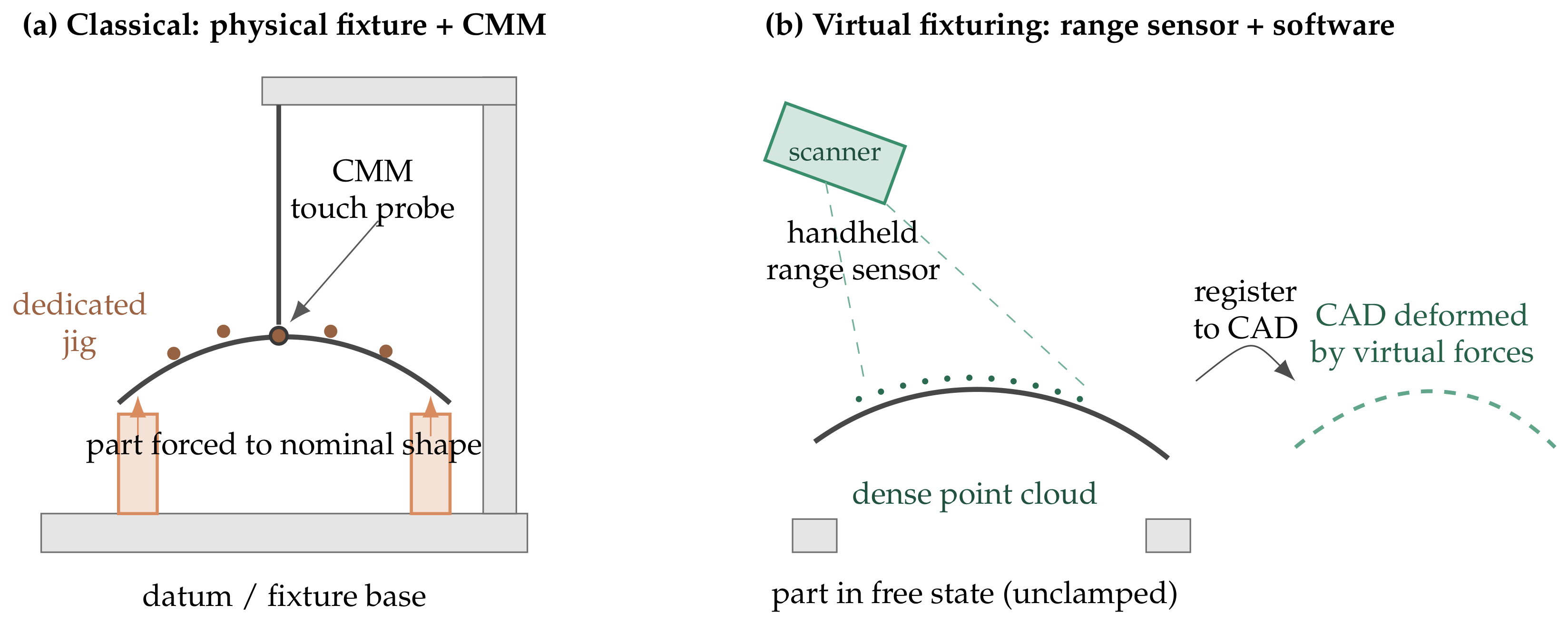
Twoclamped into a dedicated fixture that forces it to its nominal shape and fixes the datum frame, and a coordinate measuring machine probes discrete surface points by contact. (b) Virtual fixturing: the part is left in its free state and a handheld optical range sensor captures a dense point cloud of the visible surface; the nominal CAD model is then deformed to that scan in software, so the physical jig and the touch probe are replaced by a scan and a non-rigid registration.
Figure 1.
Twoclamped into a dedicated fixture that forces it to its nominal shape and fixes the datum frame, and a coordinate measuring machine probes discrete surface points by contact. (b) Virtual fixturing: the part is left in its free state and a handheld optical range sensor captures a dense point cloud of the visible surface; the nominal CAD model is then deformed to that scan in software, so the physical jig and the touch probe are replaced by a scan and a non-rigid registration.
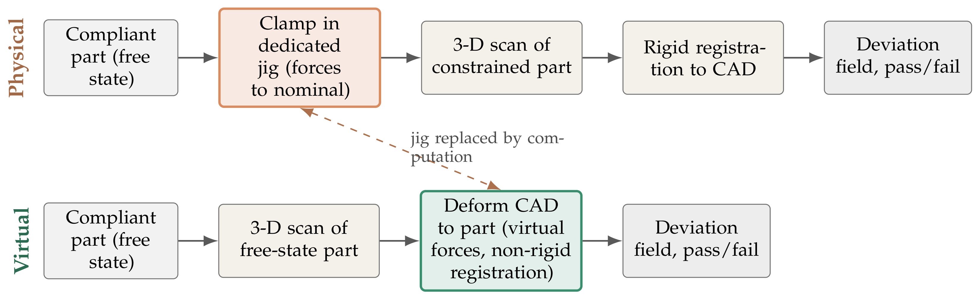
Figure 2.
Two routes to inspecting a compliant part. Physical fixturing (top) clamps the part into a dedicated jig that forces it to its nominal shape, then inspects it as a rigid part. Virtual fixturing (bottom) scans the part in its free state and instead deforms the CAD model to match the scan, replacing the part-specific jig and its manual setup with a computation. Both routes end at the same deviation-and-tolerance decision.
Figure 2.
Two routes to inspecting a compliant part. Physical fixturing (top) clamps the part into a dedicated jig that forces it to its nominal shape, then inspects it as a rigid part. Virtual fixturing (bottom) scans the part in its free state and instead deforms the CAD model to match the scan, replacing the part-specific jig and its manual setup with a computation. Both routes end at the same deviation-and-tolerance decision.
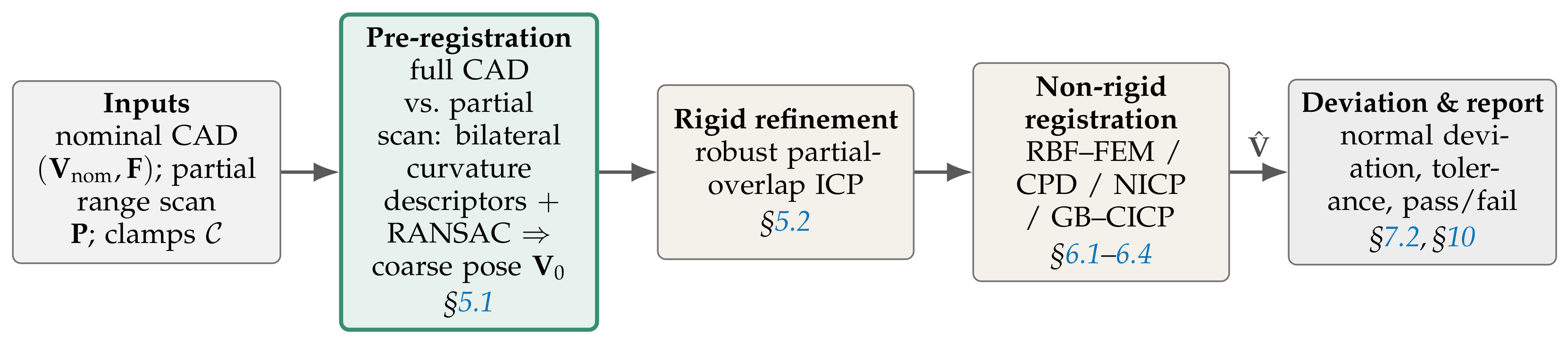
Figure 3.
Data-processing pipeline. The nominal CAD model, the scan, and the clamp indices enter a pre-registration stage (
Section 5.1) that fixes a coarse pose by matching the complete CAD model to the partial range view through geodesic bilateral curvature descriptors and RANSAC, a robust rigid refinement (
Section 5.2) seats the model on the scan and also serves as the baseline. One of four non-rigid registration algorithms then deforms the model to the scan, producing the estimated surface
, and the normal-deviation metric with the tolerance turns
into a pass/fail conformance report.
Figure 3.
Data-processing pipeline. The nominal CAD model, the scan, and the clamp indices enter a pre-registration stage (
Section 5.1) that fixes a coarse pose by matching the complete CAD model to the partial range view through geodesic bilateral curvature descriptors and RANSAC, a robust rigid refinement (
Section 5.2) seats the model on the scan and also serves as the baseline. One of four non-rigid registration algorithms then deforms the model to the scan, producing the estimated surface
, and the normal-deviation metric with the tolerance turns
into a pass/fail conformance report.
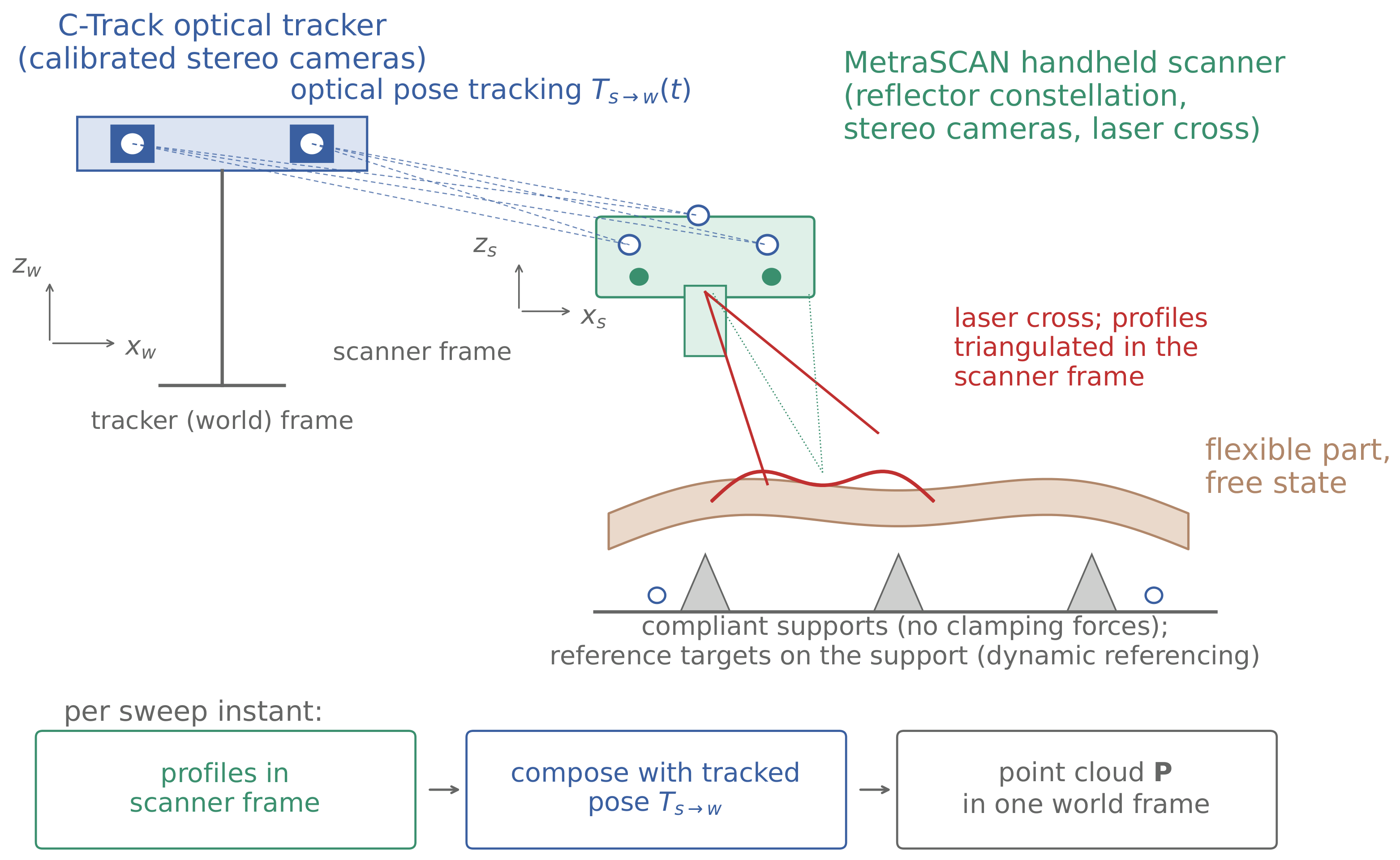
Figure 4.
Functional arrangement of an optically tracked handheld laser scanner (Creaform MetraSCAN with the C-Track tracker, drawn schematically). A fixed, calibrated stereo tracker continuously observes a constellation of reflectors on the scanner body, giving the scanner pose in the tracker (world) frame at every instant as the part itself carries no targets. The scanner projects a laser cross whose illuminated profiles are triangulated by its onboard cameras in the scanner frame, and composing each profile with the tracked pose places the points directly in the single world frame, so the accumulated cloud arrives already registered. The flexible part rests in its free state on compliant supports. Optional reference targets on the support, not the part, let the tracker compensate rigid motion (dynamic referencing).
Figure 4.
Functional arrangement of an optically tracked handheld laser scanner (Creaform MetraSCAN with the C-Track tracker, drawn schematically). A fixed, calibrated stereo tracker continuously observes a constellation of reflectors on the scanner body, giving the scanner pose in the tracker (world) frame at every instant as the part itself carries no targets. The scanner projects a laser cross whose illuminated profiles are triangulated by its onboard cameras in the scanner frame, and composing each profile with the tracked pose places the points directly in the single world frame, so the accumulated cloud arrives already registered. The flexible part rests in its free state on compliant supports. Optional reference targets on the support, not the part, let the tracker compensate rigid motion (dynamic referencing).
Figure 7.
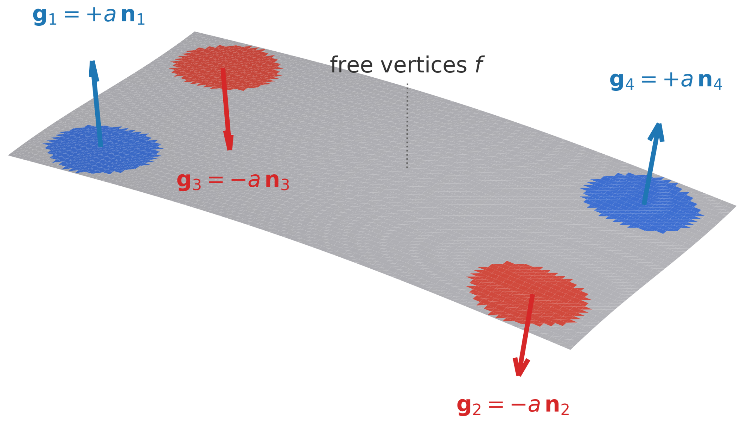
Clamping configuration used by the deformation generator. The handle vertices
(highlighted) are small patches at the fixturing locations of the part. Each handle
c is assigned a prescribed displacement
directed along the local surface normal (arrows). All remaining vertices are unconstrained, and the biharmonic energy of Equation (
2) propagates the handle motion smoothly over the rest of the mesh.
Figure 7.
Clamping configuration used by the deformation generator. The handle vertices
(highlighted) are small patches at the fixturing locations of the part. Each handle
c is assigned a prescribed displacement
directed along the local surface normal (arrows). All remaining vertices are unconstrained, and the biharmonic energy of Equation (
2) propagates the handle motion smoothly over the rest of the mesh.
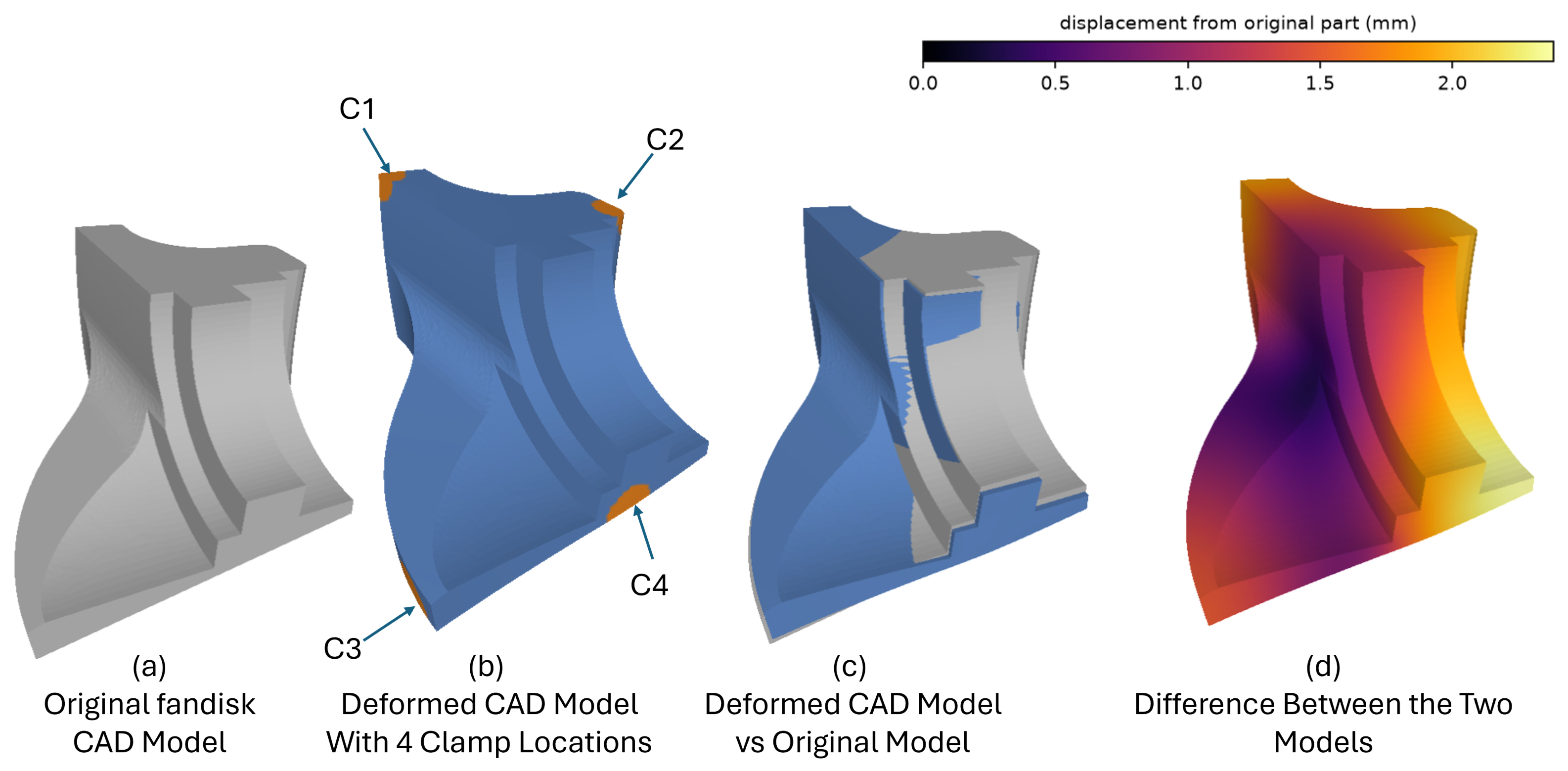
Figure 8.
Free-state generation on the fandisk CAD model. (
a) The nominal STL geometry, shaded. (
b) Location (orange) of four clamps on the deformed free state part; (
c) The deformed free state produced by the biharmonic generator (blue), overlaid on the nominal model (grey). The two surfaces separate where the prescribed handle motion drives the part away from its as-designed shape. (
d) The deformed model colored by per-vertex displacement magnitude from the nominal part (mm). The field varies smoothly across the surface, from the nearly stationary dark region at the center to more than 2 mm at the driven corners, confirming that the generated deformation is a gentle, globally coherent bending rather than a localized distortion. The recovered inspection deviation for this case is reported in
Figure 6.
Figure 8.
Free-state generation on the fandisk CAD model. (
a) The nominal STL geometry, shaded. (
b) Location (orange) of four clamps on the deformed free state part; (
c) The deformed free state produced by the biharmonic generator (blue), overlaid on the nominal model (grey). The two surfaces separate where the prescribed handle motion drives the part away from its as-designed shape. (
d) The deformed model colored by per-vertex displacement magnitude from the nominal part (mm). The field varies smoothly across the surface, from the nearly stationary dark region at the center to more than 2 mm at the driven corners, confirming that the generated deformation is a gentle, globally coherent bending rather than a localized distortion. The recovered inspection deviation for this case is reported in
Figure 6.
Figure 9.
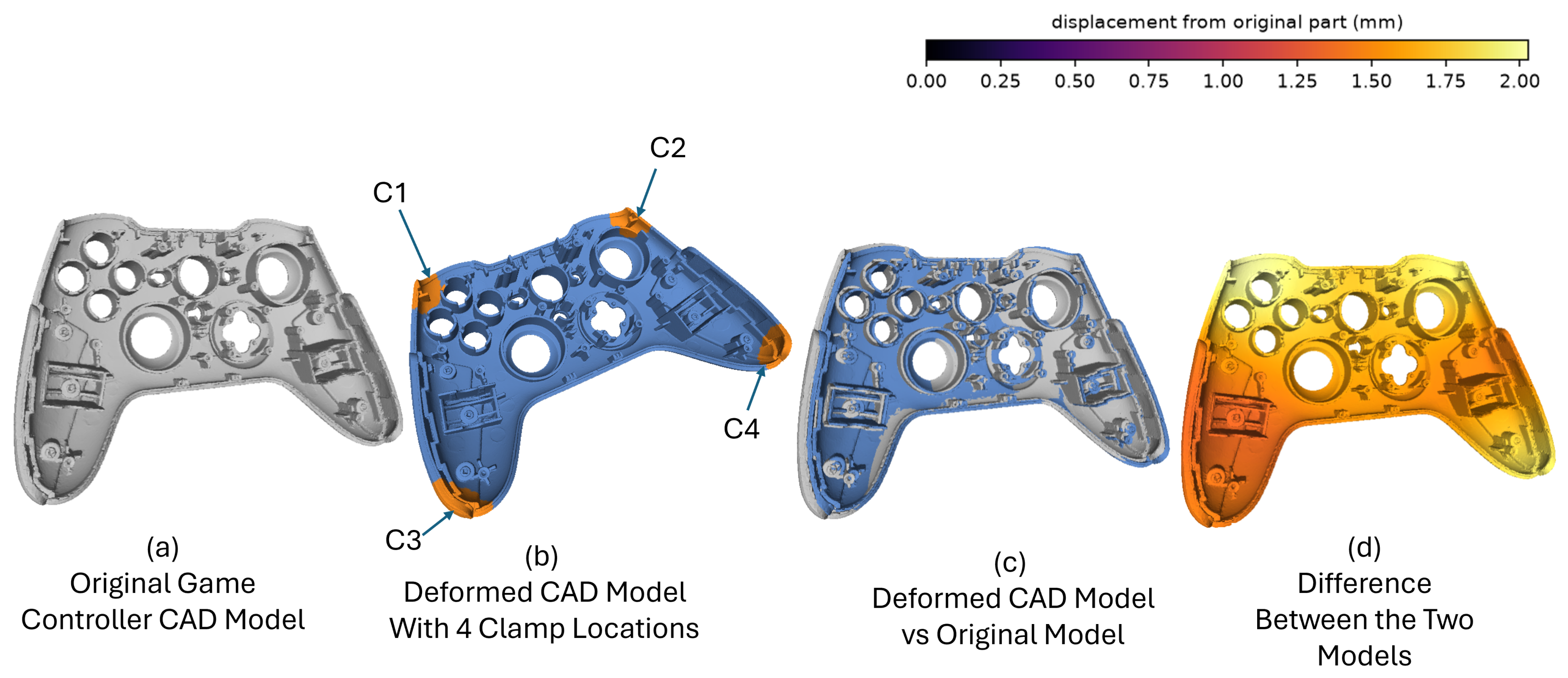
Free-state generation on the game-controller shell. (
a) The nominal STL geometry, shaded; (
b) Location (orange) of four clamps on the deformed free state part; (
c) The deformed free state (blue) overlaid on the nominal model (grey); the separation is most visible along the outer rim and the grips, where the bending mode displaces the shell furthest from its as-designed pose. (
d) The deformed model colored by per-vertex displacement magnitude from the nominal part (mm), ranging from about 1.3 mm over the central face to nearly 2 mm at the upper edge and grip tips. The smooth, monotone variation of the field across the whole shell is characteristic of the low-order bending modes produced by the generator. The recovered inspection deviation for this case is reported in
Figure 6.
Figure 9.
Free-state generation on the game-controller shell. (
a) The nominal STL geometry, shaded; (
b) Location (orange) of four clamps on the deformed free state part; (
c) The deformed free state (blue) overlaid on the nominal model (grey); the separation is most visible along the outer rim and the grips, where the bending mode displaces the shell furthest from its as-designed pose. (
d) The deformed model colored by per-vertex displacement magnitude from the nominal part (mm), ranging from about 1.3 mm over the central face to nearly 2 mm at the upper edge and grip tips. The smooth, monotone variation of the field across the whole shell is characteristic of the low-order bending modes produced by the generator. The recovered inspection deviation for this case is reported in
Figure 6.
Figure 10.
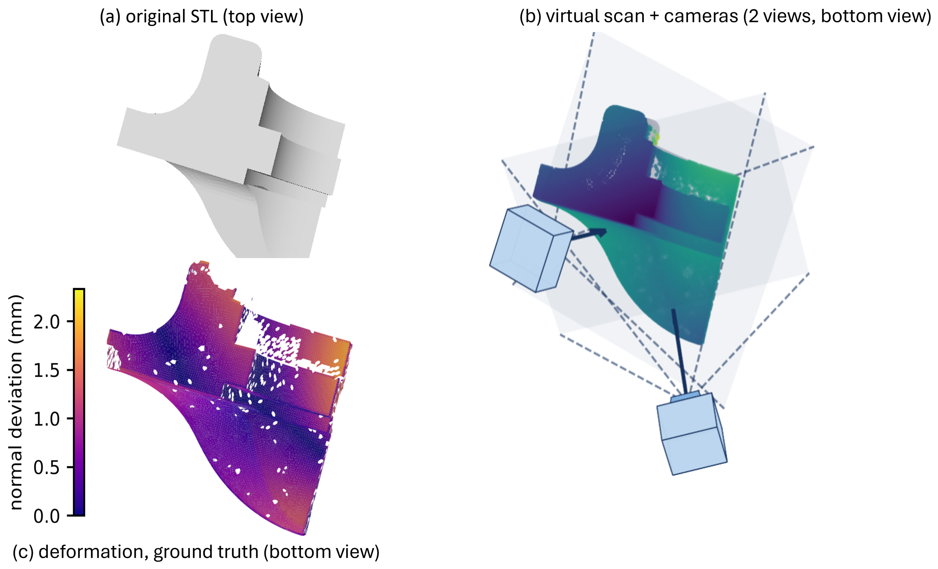
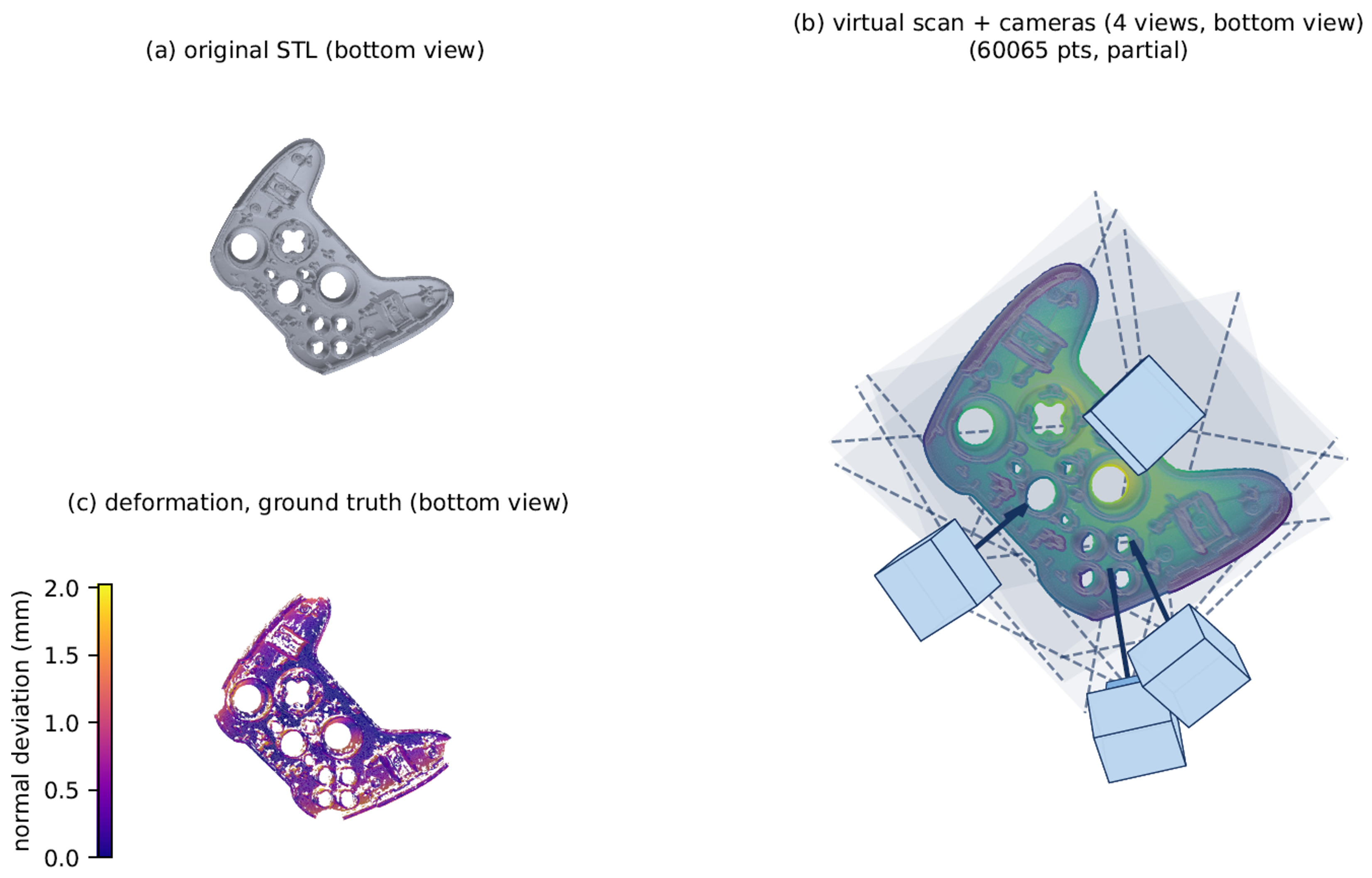
The generator pipeline on the game controller housing, a smooth, low-feature CAD part, shown from the top shell throughout. (
a) The original STL as CAD reference, shaded. (
b) A virtual scan from four viewpoints, each marked by its virtual camera and view frustum. The grips and underside remain self-occluded, leaving the characteristic missing-data regions of a fixtureless scan. (
c) A prescribed free-state deformation applied to the part and kept as exact ground truth, colored by normal deviation. The recovered inspection deviation for this case is reported in
Figure 6.
Figure 10.
The generator pipeline on the game controller housing, a smooth, low-feature CAD part, shown from the top shell throughout. (
a) The original STL as CAD reference, shaded. (
b) A virtual scan from four viewpoints, each marked by its virtual camera and view frustum. The grips and underside remain self-occluded, leaving the characteristic missing-data regions of a fixtureless scan. (
c) A prescribed free-state deformation applied to the part and kept as exact ground truth, colored by normal deviation. The recovered inspection deviation for this case is reported in
Figure 6.
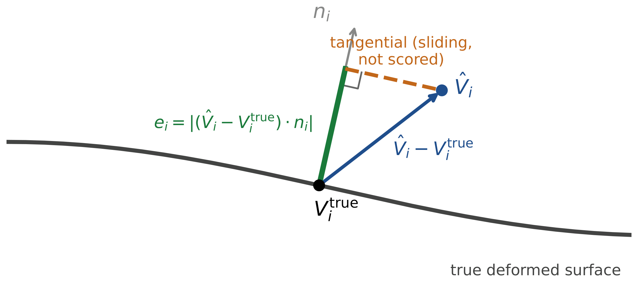
Figure 11.
How the inspection deviation is computed. For corresponding vertices on the estimated surface and the true deformed surface , the residual is split into its component along the surface normal , the scored deviation , and a tangential component. Tangential sliding leaves the surface where it belongs and cannot be observed from surface points, so it is not counted as deviation.
Figure 11.
How the inspection deviation is computed. For corresponding vertices on the estimated surface and the true deformed surface , the residual is split into its component along the surface normal , the scored deviation , and a tangential component. Tangential sliding leaves the surface where it belongs and cannot be observed from surface points, so it is not counted as deviation.
Figure 12.
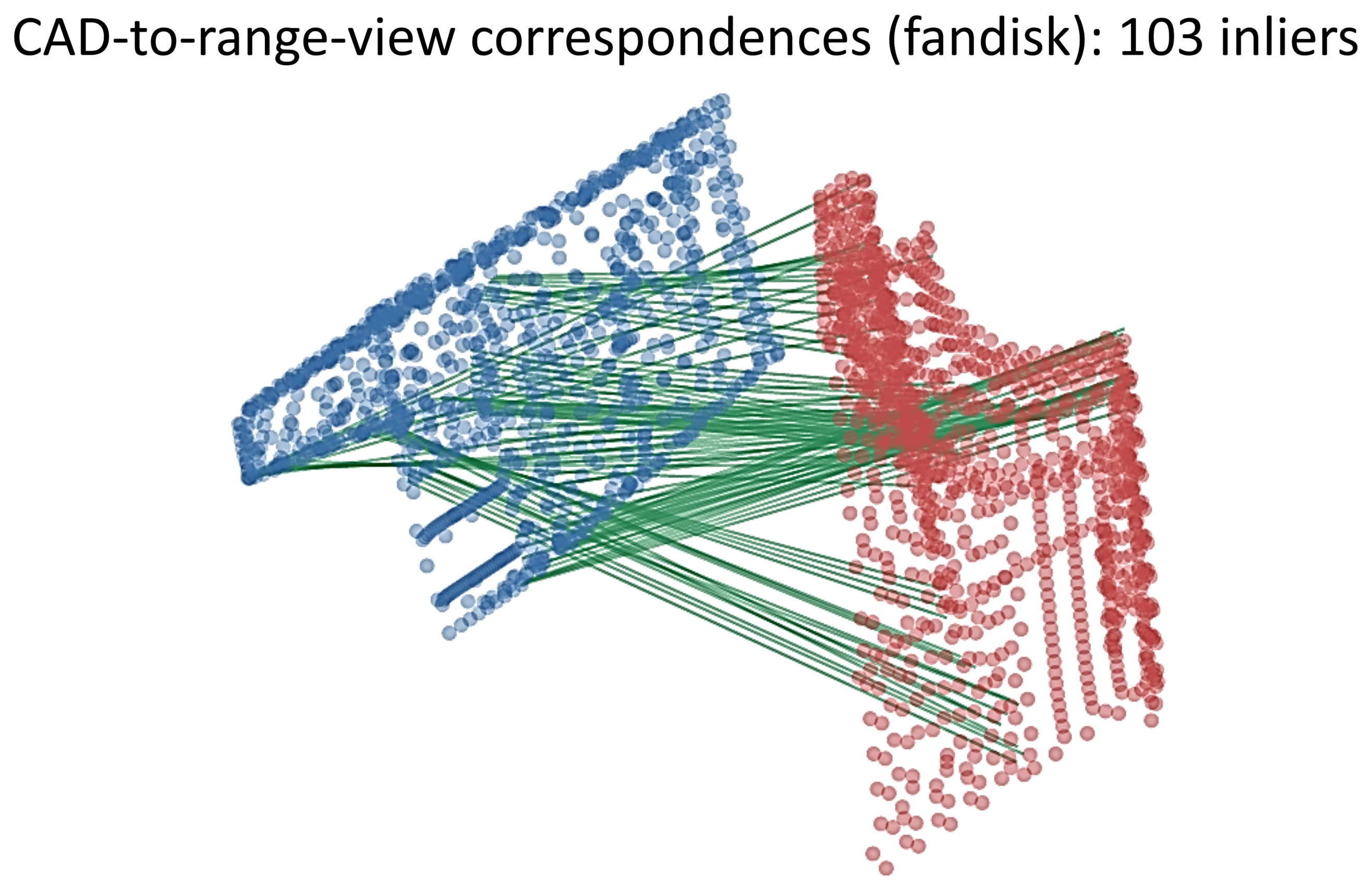
Pre-registration on the fandisk between the full nominal CAD model (blue) and a partial, noisy range-sensor view (red, 51% surface coverage, two views, 0.02 mm noise) of the part at a known 121.4° pose. Green segments are the bilateral curvature descriptor matches retained as RANSAC inliers. The descriptor is built from intrinsic curvature and is invariant to the rigid pose. The construction follows [
65] and the run is computed with the toolkit.
Figure 12.
Pre-registration on the fandisk between the full nominal CAD model (blue) and a partial, noisy range-sensor view (red, 51% surface coverage, two views, 0.02 mm noise) of the part at a known 121.4° pose. Green segments are the bilateral curvature descriptor matches retained as RANSAC inliers. The descriptor is built from intrinsic curvature and is invariant to the rigid pose. The construction follows [
65] and the run is computed with the toolkit.
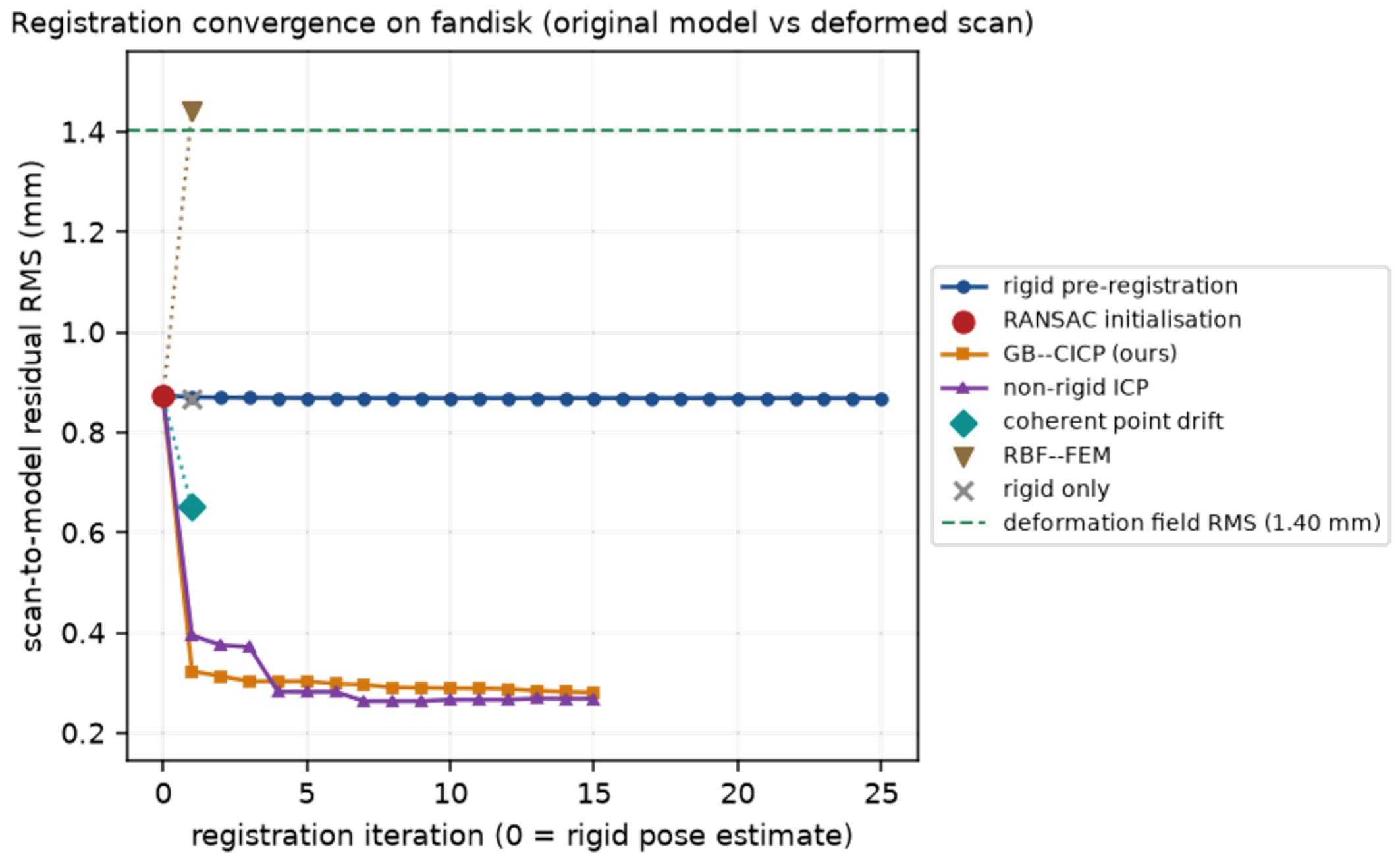
Figure 13.
Convergence of the CAD-to-range-view registration on the fandisk (original model vs. deformed scan). The coarse RANSAC pose starts the refinement at a scan-to-model RMS of 0.87 mm, and rigid ICP settles within the first iterations onto a 0.86 mm plateau—the floor attainable by any rigid transform, since the part carries a deformation field of 1.40 mm RMS (dashed). From this rigid estimate the proposed GB–CICP reduces the residual to 0.28 mm, on par with non-rigid ICP (0.26 mm), while coherent point drift stalls at 0.65 mm and RBF–FEM overshoots to 1.45 mm. This run represents the partial-overlap operating point of the pipeline. The complementary full-mesh rigid-recovery validation of the descriptor in [
65] reaches the floating-point floor.
Figure 13.
Convergence of the CAD-to-range-view registration on the fandisk (original model vs. deformed scan). The coarse RANSAC pose starts the refinement at a scan-to-model RMS of 0.87 mm, and rigid ICP settles within the first iterations onto a 0.86 mm plateau—the floor attainable by any rigid transform, since the part carries a deformation field of 1.40 mm RMS (dashed). From this rigid estimate the proposed GB–CICP reduces the residual to 0.28 mm, on par with non-rigid ICP (0.26 mm), while coherent point drift stalls at 0.65 mm and RBF–FEM overshoots to 1.45 mm. This run represents the partial-overlap operating point of the pipeline. The complementary full-mesh rigid-recovery validation of the descriptor in [
65] reaches the floating-point floor.
Figure 14.
Rigid pre-registration of the fandisk. (
Left): the complete CAD model (grey) and the partial range-sensor view (red) before alignment, each in its own frame. (
Right): after applying the recovered pose
, the scanned region of the CAD model is Phong-shaded by its per-vertex difference to the registered scan. Because the scanned part is deformed, the residual does not vanish under the rigid pose: it sits at the 0.86 mm RMS rigid floor of
Figure 13, concentrated where the 1.40 mm RMS deformation field displaces the surface, well above the 0.02 mm scan noise. This residual map is exactly the signal handed to the deformable stage. Computed with the toolkit.
Figure 14.
Rigid pre-registration of the fandisk. (
Left): the complete CAD model (grey) and the partial range-sensor view (red) before alignment, each in its own frame. (
Right): after applying the recovered pose
, the scanned region of the CAD model is Phong-shaded by its per-vertex difference to the registered scan. Because the scanned part is deformed, the residual does not vanish under the rigid pose: it sits at the 0.86 mm RMS rigid floor of
Figure 13, concentrated where the 1.40 mm RMS deformation field displaces the surface, well above the 0.02 mm scan noise. This residual map is exactly the signal handed to the deformable stage. Computed with the toolkit.
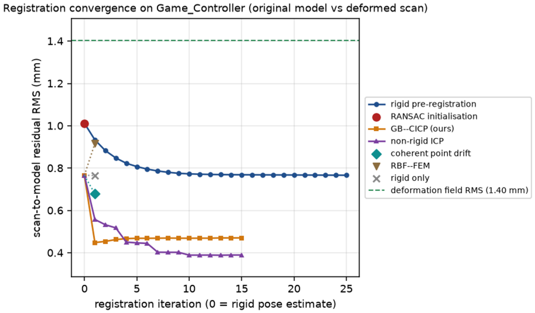
Figure 15.
Convergence of the CAD-to-range-view registration on the controller (original model vs. deformed scan). With only 10 RANSAC inliers on this descriptor-poor surface, the coarse pose starts the refinement at 7.9 mm RMS, and rigid ICP decays over some 25 iterations onto the 1.4 mm plateau set by the part’s deformation field (1.44 mm RMS, dashed)—slower than the fandisk’s near-immediate settling, but to the same kind of rigid floor. From this estimate the deformable entrants reduce the scan-to-model residual further, GB–CICP and non-rigid ICP settling lowest within a few iterations while coherent point drift and RBF–FEM stall above them.
Figure 15.
Convergence of the CAD-to-range-view registration on the controller (original model vs. deformed scan). With only 10 RANSAC inliers on this descriptor-poor surface, the coarse pose starts the refinement at 7.9 mm RMS, and rigid ICP decays over some 25 iterations onto the 1.4 mm plateau set by the part’s deformation field (1.44 mm RMS, dashed)—slower than the fandisk’s near-immediate settling, but to the same kind of rigid floor. From this estimate the deformable entrants reduce the scan-to-model residual further, GB–CICP and non-rigid ICP settling lowest within a few iterations while coherent point drift and RBF–FEM stall above them.
Figure 16.
Rigid pre-registration of the controller, produced by the released driver as in
Figure 14. (
Left): the complete CAD model and the partial range view before alignment. (
Right): the scanned region of the CAD model shaded by its per-vertex difference to the registered scan. Because the scanned part is deformed, the residual does not vanish under the rigid pose: it sits at the 1.4 mm RMS rigid floor of
Figure 15, concentrated where the 1.44 mm RMS deformation field displaces the surface. This residual map is the signal handed to the deformable stage.
Figure 16.
Rigid pre-registration of the controller, produced by the released driver as in
Figure 14. (
Left): the complete CAD model and the partial range view before alignment. (
Right): the scanned region of the CAD model shaded by its per-vertex difference to the registered scan. Because the scanned part is deformed, the residual does not vanish under the rigid pose: it sits at the 1.4 mm RMS rigid floor of
Figure 15, concentrated where the 1.44 mm RMS deformation field displaces the surface. This residual map is the signal handed to the deformable stage.
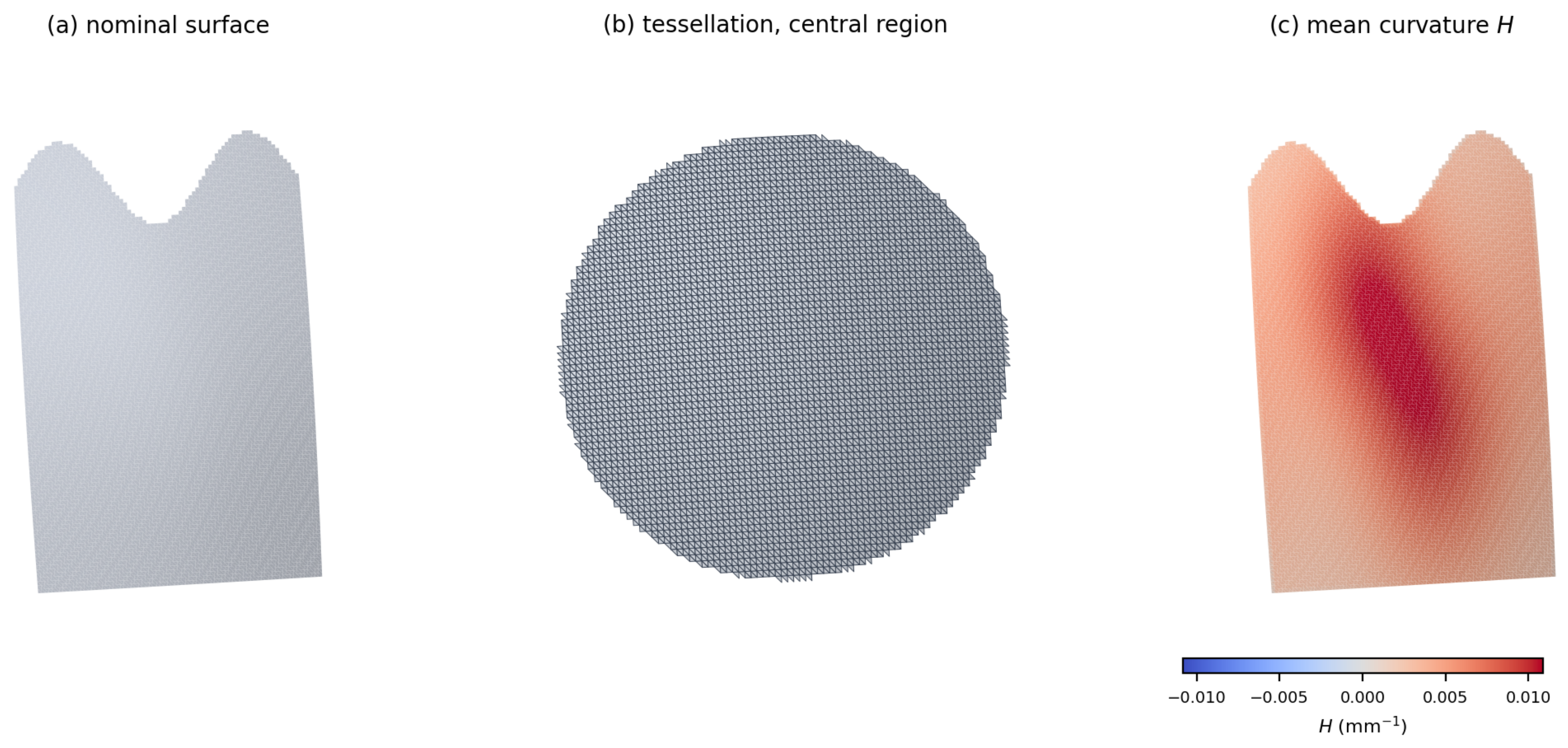
Figure 17.
The thin-shell host geometry of the detectability study. (a) The nominal surface, a doubly curved open shell of 174 × 110 × 42 mm carrying 19,144 mm2 of area on 16,650 triangles. (b) The tessellation over the central region. The median edge length of 1.894 mm is 0.90% of the bounding diagonal, so the narrowest defect in the grid spans about three elements. (c) Mean curvature H, with a median magnitude of 5.2 × 10⁻³ mm−1 corresponding to a radius of about 192 mm. The near-vanishing Gaussian curvature, = 2.6 × 10⁻⁵ mm−2, makes the surface nearly developable and free of creases, so a defect is resolved against a smooth background rather than against surface detail.
Figure 17.
The thin-shell host geometry of the detectability study. (a) The nominal surface, a doubly curved open shell of 174 × 110 × 42 mm carrying 19,144 mm2 of area on 16,650 triangles. (b) The tessellation over the central region. The median edge length of 1.894 mm is 0.90% of the bounding diagonal, so the narrowest defect in the grid spans about three elements. (c) Mean curvature H, with a median magnitude of 5.2 × 10⁻³ mm−1 corresponding to a radius of about 192 mm. The near-vanishing Gaussian curvature, = 2.6 × 10⁻⁵ mm−2, makes the surface nearly developable and free of creases, so a defect is resolved against a smooth background rather than against surface detail.
Figure 18.
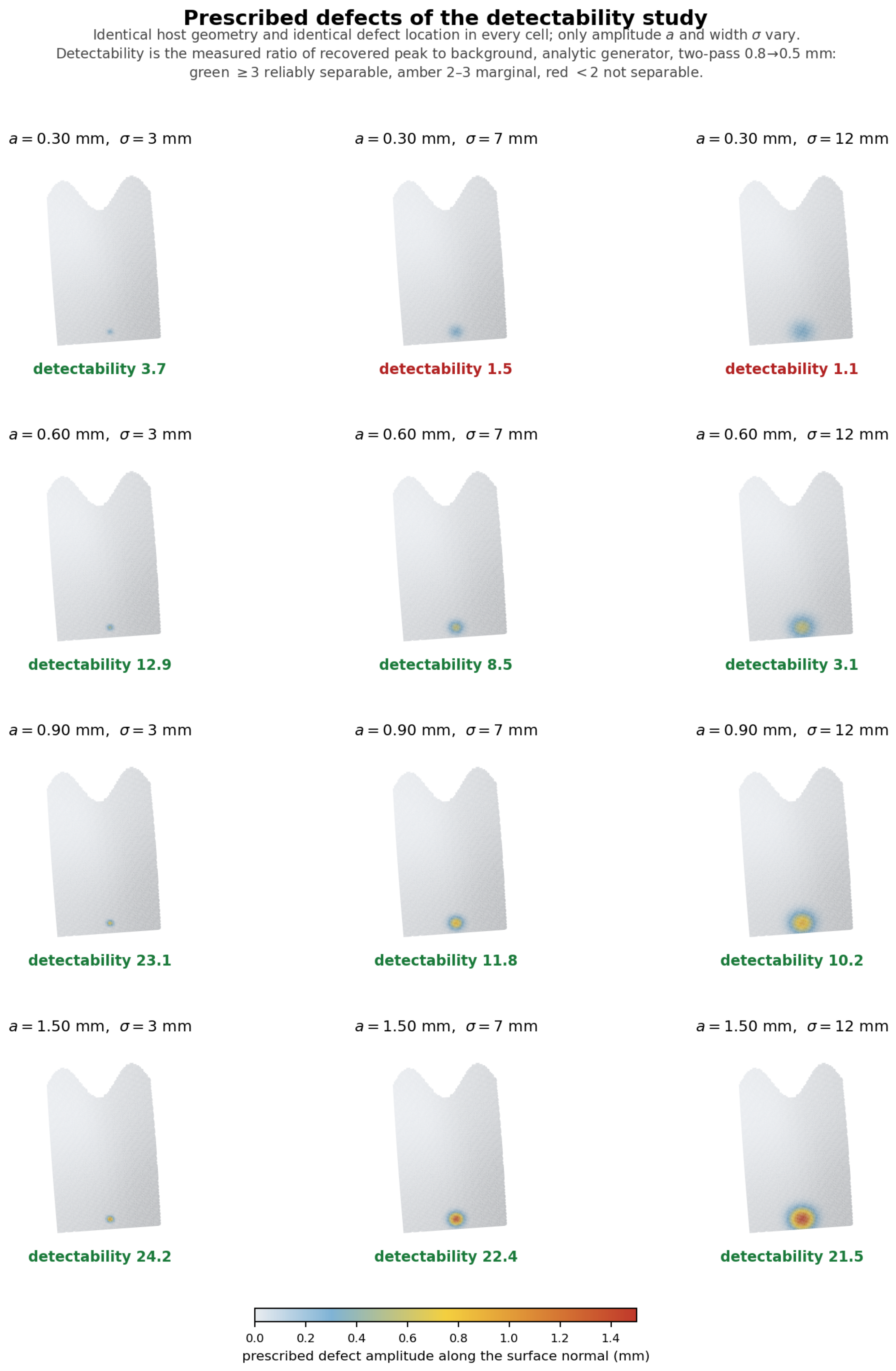
The twelve prescribed defects of
Table 3, shown on the host geometry. The part, the free-state deformation and the defect location are identical in every cell. Only the amplitude
a and the width
vary, so the grid isolates those two parameters. Color is the prescribed displacement along the surface normal on a common scale, so amplitude is read from the color and width from the extent of the colored region. The figure beneath each panel is the measured detectability ratio under the analytic generator: green where the defect is reliably separable from the background, amber where it is marginal, red where it is not separable at all. Reading down a column shows detectability improving with amplitude at fixed width; reading across a row shows it degrading with width at fixed amplitude, which is the asymmetry the band-limit predicts and the principal limitation of the approach.
Figure 18.
The twelve prescribed defects of
Table 3, shown on the host geometry. The part, the free-state deformation and the defect location are identical in every cell. Only the amplitude
a and the width
vary, so the grid isolates those two parameters. Color is the prescribed displacement along the surface normal on a common scale, so amplitude is read from the color and width from the extent of the colored region. The figure beneath each panel is the measured detectability ratio under the analytic generator: green where the defect is reliably separable from the background, amber where it is marginal, red where it is not separable at all. Reading down a column shows detectability improving with amplitude at fixed width; reading across a row shows it degrading with width at fixed amplitude, which is the asymmetry the band-limit predicts and the principal limitation of the approach.
Figure 19.
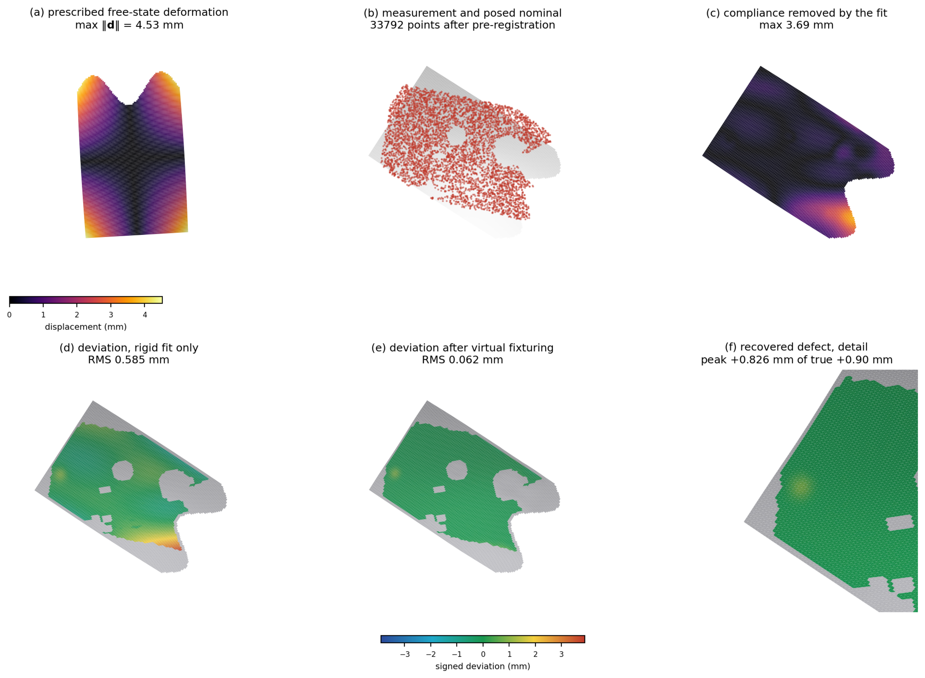
One cell of the detectability grid,
= 0.90 mm at
= 7 mm, carried through the pipeline on the thin-shell geometry of
Section 8.3.1. (
a) The prescribed free-state deformation, magnitude up to 4.53 mm, drawn from the analytic generator so that it is the minimizer of no method’s regularizer. (
b) The simulated measurement, 33,792 points retained, shown with the nominal after pre-registration. (
c) The compliance the band-limited two-pass fit removed, up to 3.69 mm. (
d) The deviation reported by a rigid best fit, 0.585 mm RMS: the free-state deflection is charged to the part and the defect is not distinguishable within it. (
e) The deviation after virtual fixturing, 0.062 mm RMS, on the same color scale. (
f) Detail at the defect, recovered at +0.826 mm against a true amplitude of +0.90 mm. Grey denotes surface outside the coverage mask or within the excluded boundary band.
Figure 19.
One cell of the detectability grid,
= 0.90 mm at
= 7 mm, carried through the pipeline on the thin-shell geometry of
Section 8.3.1. (
a) The prescribed free-state deformation, magnitude up to 4.53 mm, drawn from the analytic generator so that it is the minimizer of no method’s regularizer. (
b) The simulated measurement, 33,792 points retained, shown with the nominal after pre-registration. (
c) The compliance the band-limited two-pass fit removed, up to 3.69 mm. (
d) The deviation reported by a rigid best fit, 0.585 mm RMS: the free-state deflection is charged to the part and the defect is not distinguishable within it. (
e) The deviation after virtual fixturing, 0.062 mm RMS, on the same color scale. (
f) Detail at the defect, recovered at +0.826 mm against a true amplitude of +0.90 mm. Grey denotes surface outside the coverage mask or within the excluded boundary band.
Figure 20.
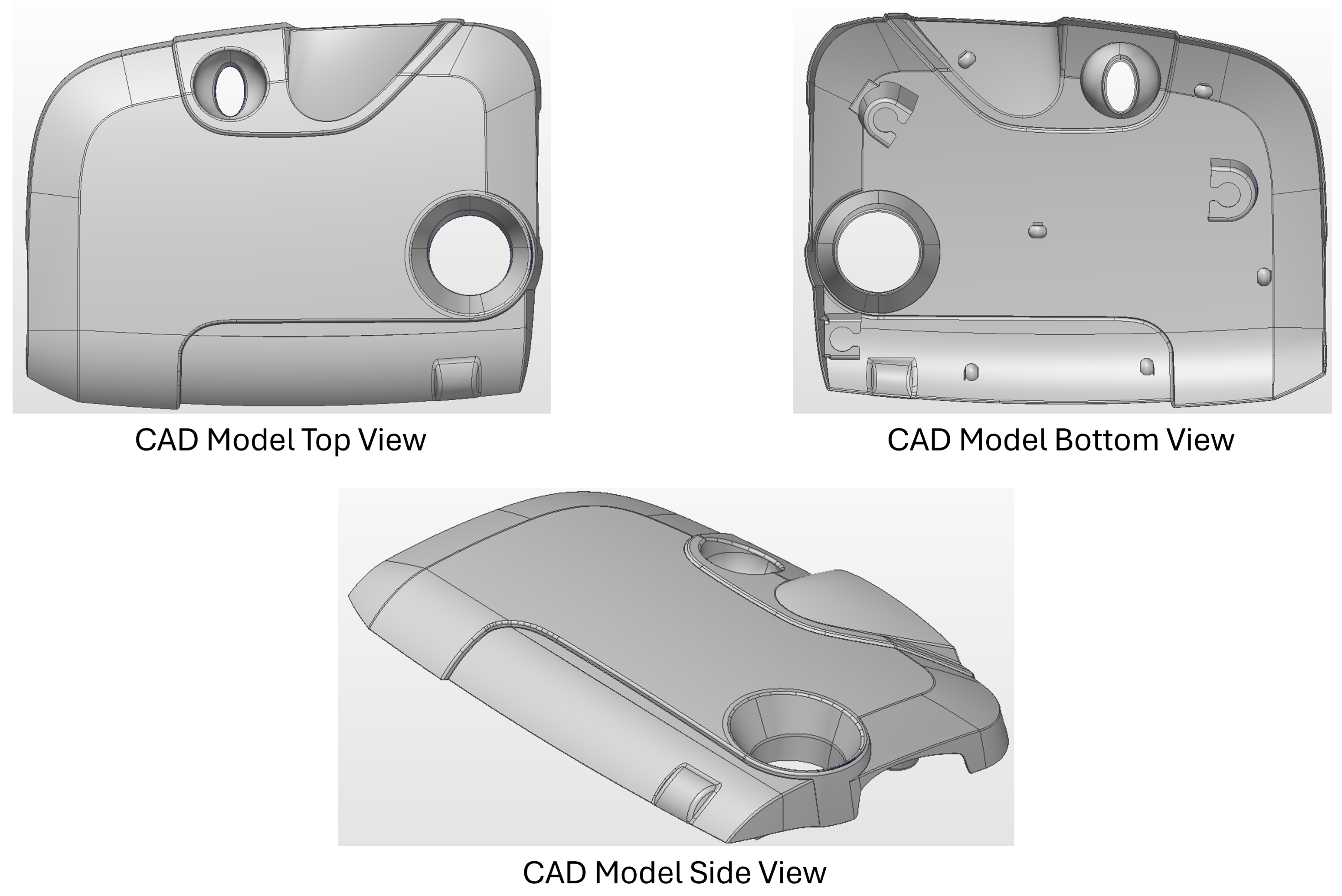
The nominal CAD model of the injection-molded engine cover used for the physical experiment, shown from the top, the bottom, and in an oblique view. The part is a large, thin molding, 612 mm across its bounding diagonal, of the compliant class that fixtureless inspection targets.
Figure 20.
The nominal CAD model of the injection-molded engine cover used for the physical experiment, shown from the top, the bottom, and in an oblique view. The part is a large, thin molding, 612 mm across its bounding diagonal, of the compliant class that fixtureless inspection targets.
Figure 21.
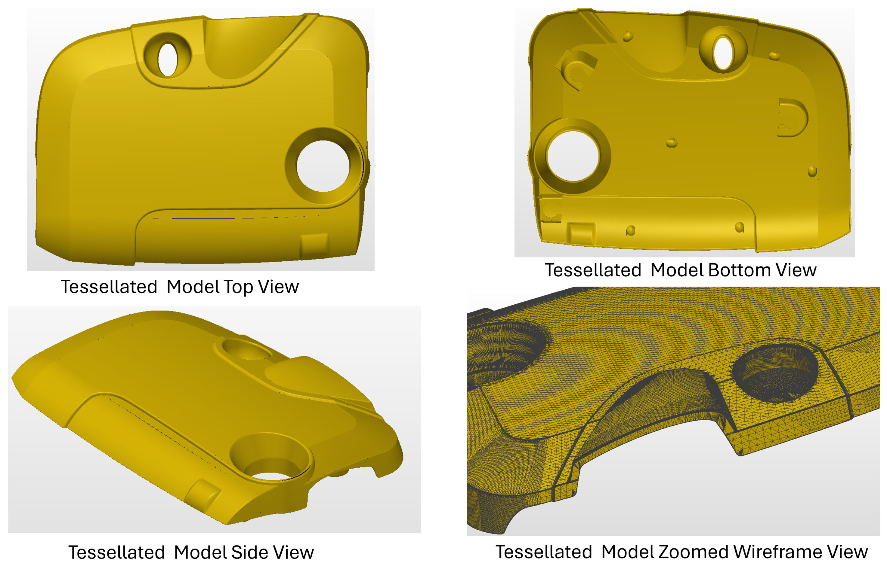
The tessellation of the nominal model, with a zoomed wireframe view. The model is delivered as an unwelded triangle soup of 115,093 vertices for 227,523 triangles, three per triangle, and is welded to the same tolerance as the nominal surface.
Figure 21.
The tessellation of the nominal model, with a zoomed wireframe view. The model is delivered as an unwelded triangle soup of 115,093 vertices for 227,523 triangles, three per triangle, and is welded to the same tolerance as the nominal surface.
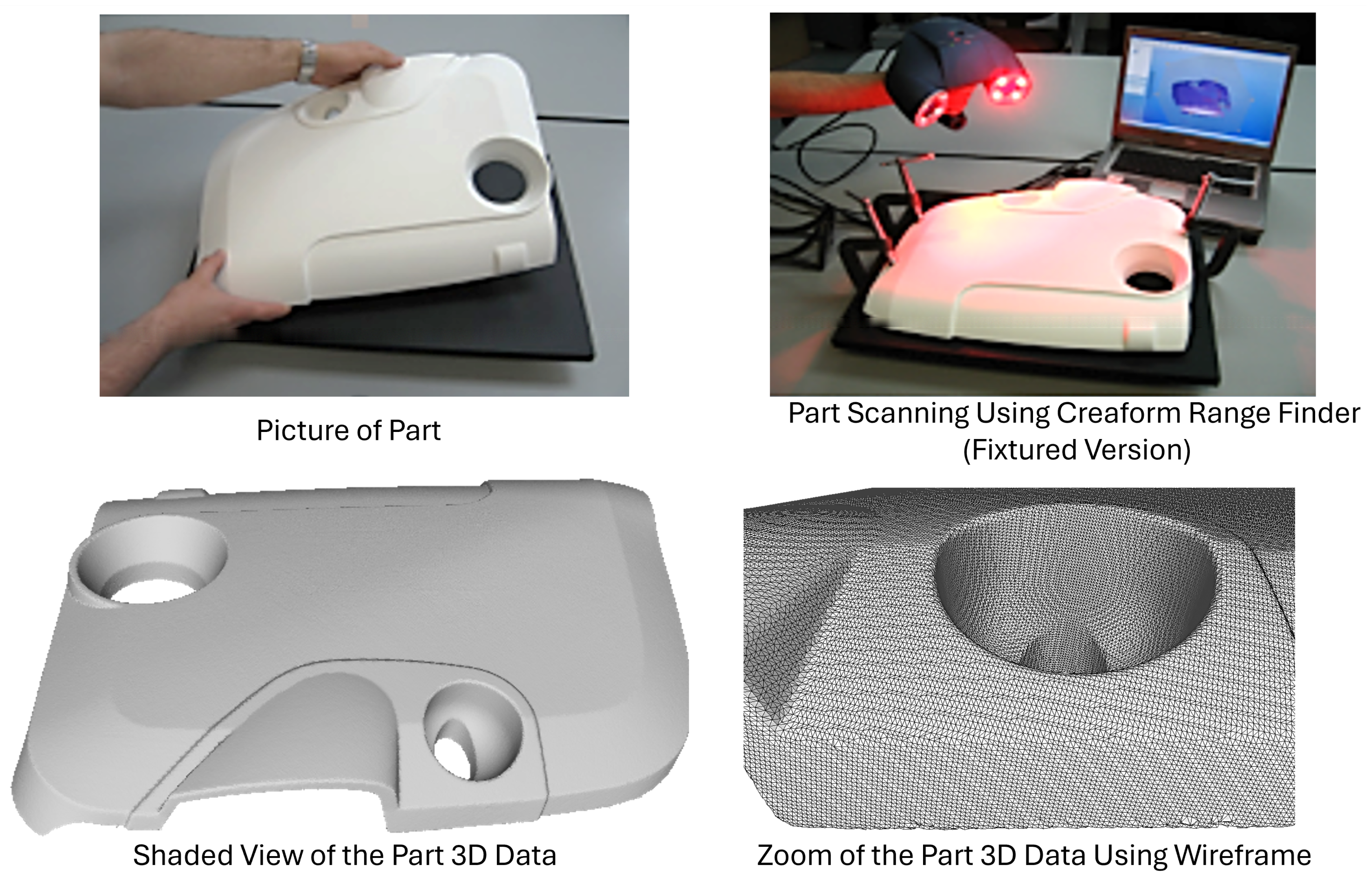
Figure 22.
Physical acquisition. The molded part, the Creaform hand-held range sensor in use, and the resulting measured surface shown shaded and in wireframe. The scan carries 373,510 triangles over 195,677 mm2 at a native resolution of 0.975 mm, with an estimated noise floor of 0.010 mm (one standard deviation) from the residual of local plane fits.
Figure 22.
Physical acquisition. The molded part, the Creaform hand-held range sensor in use, and the resulting measured surface shown shaded and in wireframe. The scan carries 373,510 triangles over 195,677 mm2 at a native resolution of 0.975 mm, with an estimated noise floor of 0.010 mm (one standard deviation) from the residual of local plane fits.
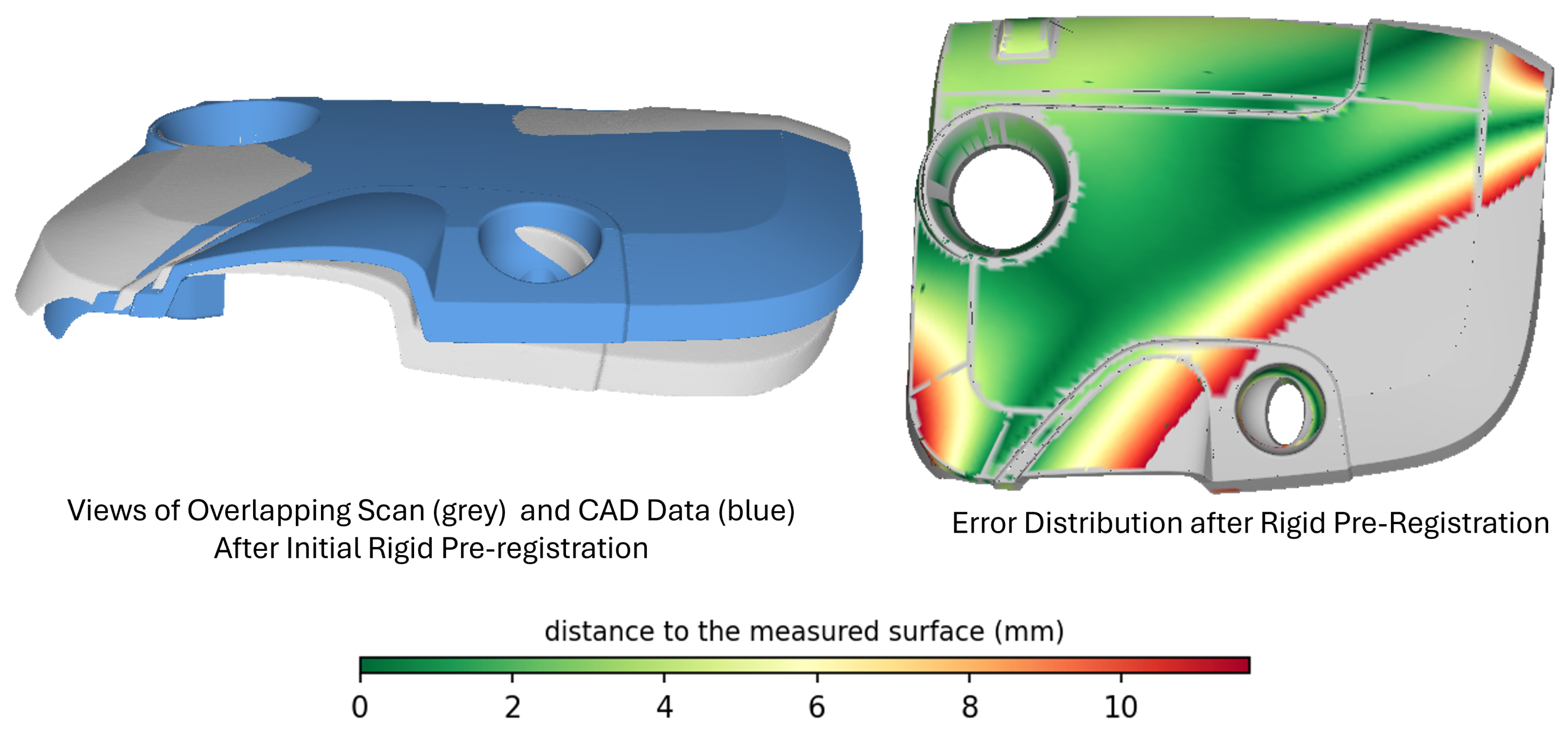
Figure 23.
Rigid pre-registration on the physical part. (Left): the measured surface and the nominal model after coarse alignment and rigid refinement. (Right): the residual distance field. The trimmed residual of 4.62 mm is the part’s free-state deflection rather than registration error: twenty independent restarts converge to the same basin within 0.01 mm, while the median restart ends at 10.4 mm, and further iteration increases the residual.
Figure 23.
Rigid pre-registration on the physical part. (Left): the measured surface and the nominal model after coarse alignment and rigid refinement. (Right): the residual distance field. The trimmed residual of 4.62 mm is the part’s free-state deflection rather than registration error: twenty independent restarts converge to the same basin within 0.01 mm, while the median restart ends at 10.4 mm, and further iteration increases the residual.
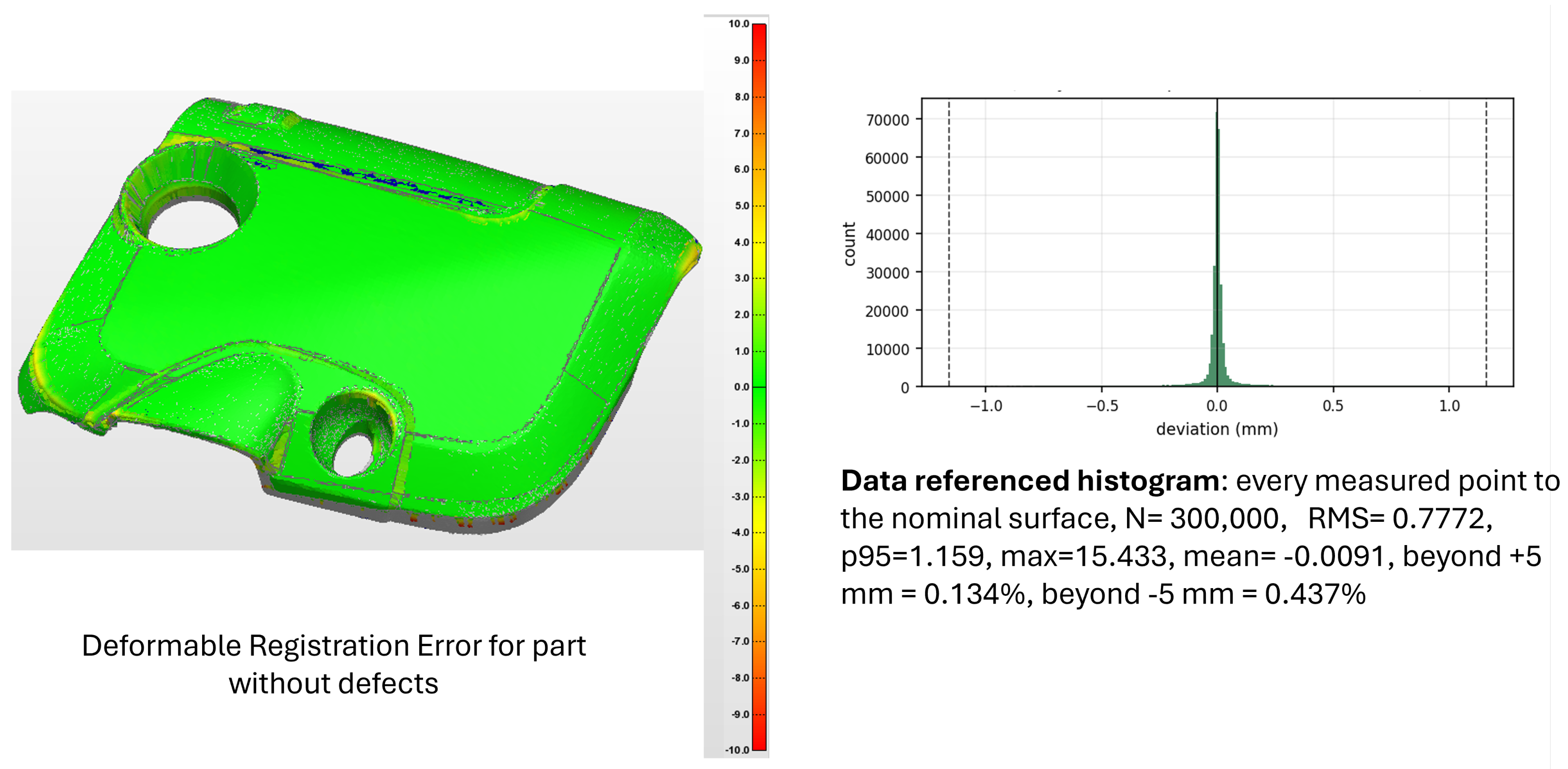
Figure 24.
Deviationfield and data-referenced histogram on the part as manufactured, after the deformable stage. Over 300,000 area-uniform samples the deviation has an RMS of 0.777 mm, a 95th percentile of 1.159 mm, a mean of −0.009 mm, and a maximum of 15.4 mm, with 0.134% beyond +5 mm and 0.437% beyond −5 mm. In the absence of a calibrated artifact this residual contains the part’s form error, the residual registration error, and the sensor noise, which are not separable.
Figure 24.
Deviationfield and data-referenced histogram on the part as manufactured, after the deformable stage. Over 300,000 area-uniform samples the deviation has an RMS of 0.777 mm, a 95th percentile of 1.159 mm, a mean of −0.009 mm, and a maximum of 15.4 mm, with 0.134% beyond +5 mm and 0.437% beyond −5 mm. In the absence of a calibrated artifact this residual contains the part’s form error, the residual registration error, and the sensor noise, which are not separable.
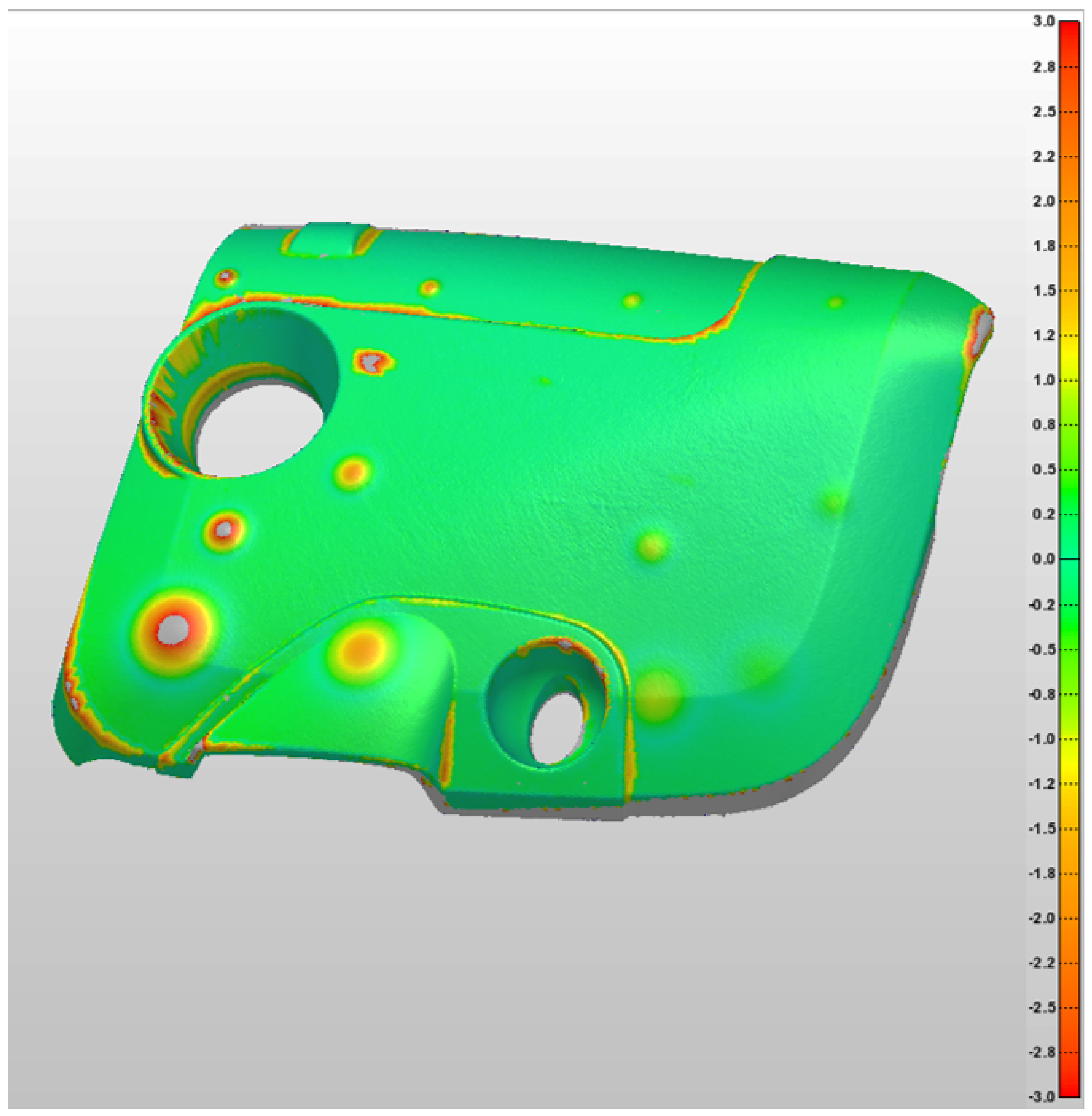
Figure 25.
Defect recovery on the physically scanned part. The twelve cells are in local residuals of 0.009 to 0.126 mm, and 11 of the 12 recover between 99 and 107 percent of their prescribed amplitude, including a defect of 0.5 mm recovered at 102 percent against a local background of 0.033 mm.
Figure 25.
Defect recovery on the physically scanned part. The twelve cells are in local residuals of 0.009 to 0.126 mm, and 11 of the 12 recover between 99 and 107 percent of their prescribed amplitude, including a defect of 0.5 mm recovered at 102 percent against a local background of 0.033 mm.
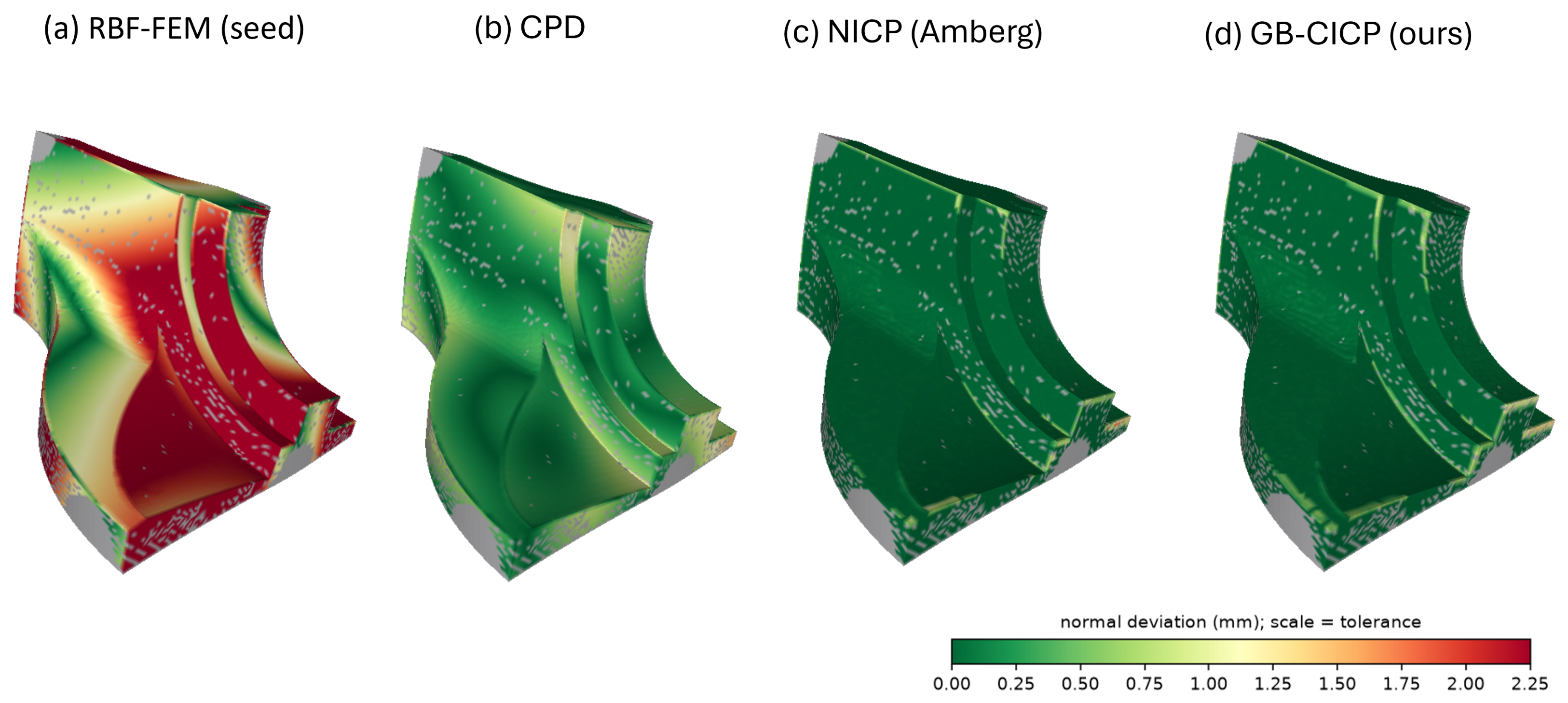
Figure 26.
The four deformable-stage entrants on the game-controller housing, the second real-CAD example alongside the fandisk of
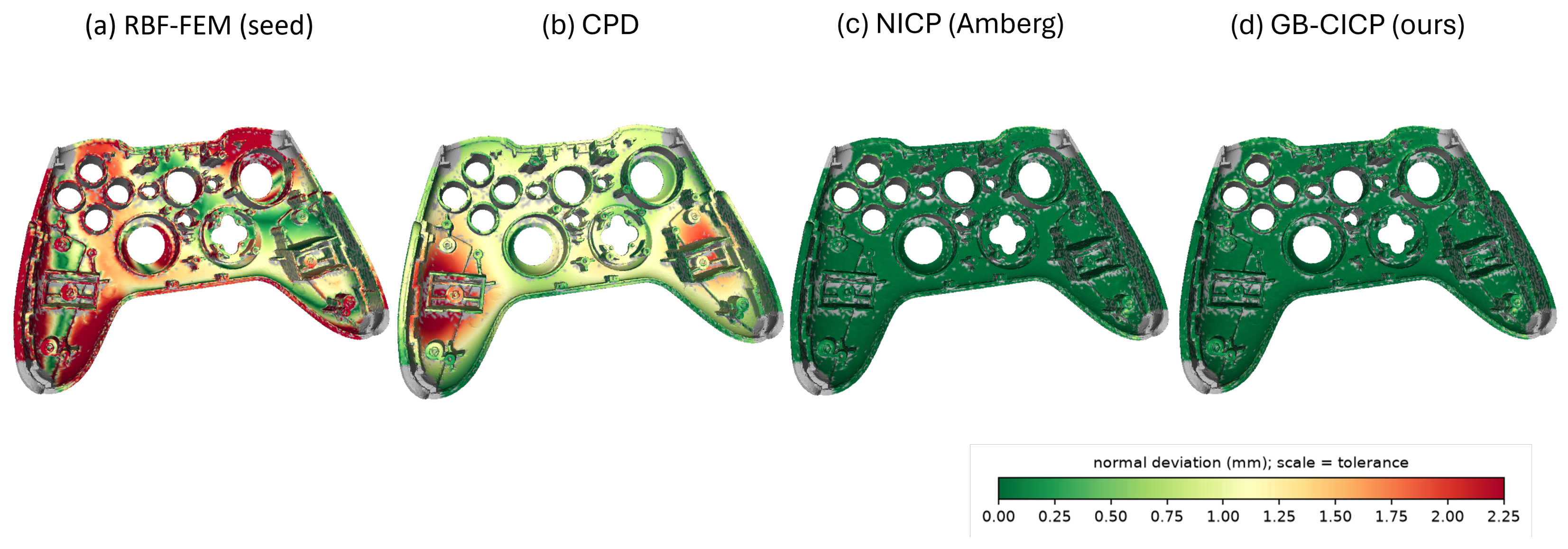
Figure 6. Because the scan is a one-sided surface, deviation is measured along the surface normal—the quantity a deviation report uses—so tangential sliding, which leaves the surface in place and which no point-based method can observe, is correctly excluded. GB–CICP (0.12 mm RMS) and NICP (0.14 mm) recover the surface almost exactly; CPD (0.76 mm) leaves visible residual; and RBF–FEM, starved by the data deliberately missing at the clamps, fails outright (2.67 mm RMS, 7.31 mm maximum). Only the vertices the scanner measured are scored, so occluded regions appear as gaps rather than as spurious deviation.
Figure 26.
The four deformable-stage entrants on the game-controller housing, the second real-CAD example alongside the fandisk of
Figure 6. Because the scan is a one-sided surface, deviation is measured along the surface normal—the quantity a deviation report uses—so tangential sliding, which leaves the surface in place and which no point-based method can observe, is correctly excluded. GB–CICP (0.12 mm RMS) and NICP (0.14 mm) recover the surface almost exactly; CPD (0.76 mm) leaves visible residual; and RBF–FEM, starved by the data deliberately missing at the clamps, fails outright (2.67 mm RMS, 7.31 mm maximum). Only the vertices the scanner measured are scored, so occluded regions appear as gaps rather than as spurious deviation.
Figure 27.
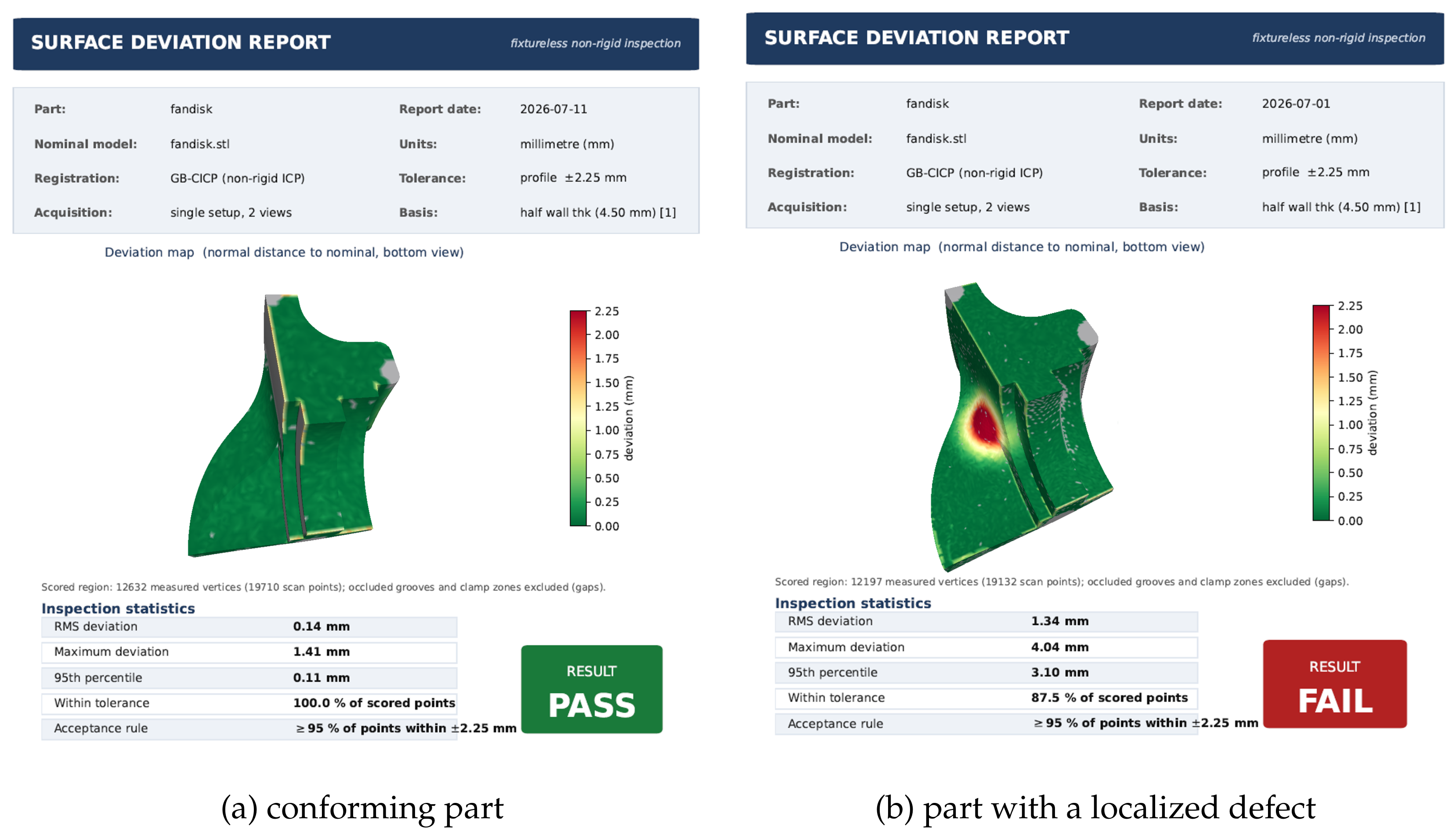
Example surface-deviation reports for the fandisk, assembled from the pipeline output. (
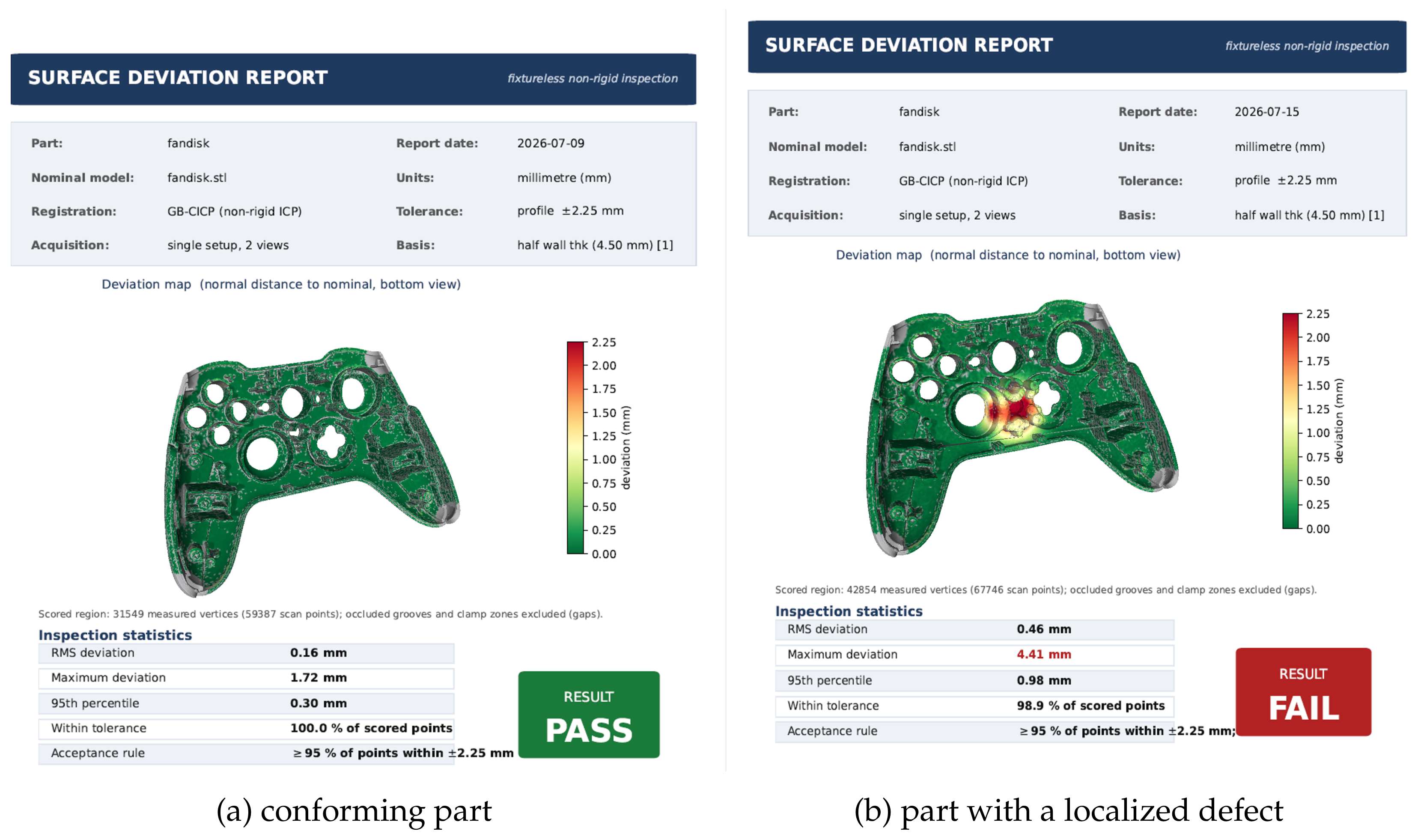
a) The as-modeled part conforms: once the compliant distortion is registered out, every scored point lies within the profile band and the verdict is pass. (
b) The same part carrying a raised boss that is not a compliant deformation: it survives the registration as residual form error, exceeds the band over a clear region, drops the in-tolerance fraction below the acceptance threshold, and the verdict is fail. Both reports are produced by the GB–CICP registration of
Section 6.4. Detecting such defects depends on the registration being limited to the part’s compliant modes so that it removes the fixturing distortion without absorbing the defect. A maximally flexible fit would mask it. The tolerance band, deviation map, statistics, and verdict are the report components described above.
Figure 27.
Example surface-deviation reports for the fandisk, assembled from the pipeline output. (
a) The as-modeled part conforms: once the compliant distortion is registered out, every scored point lies within the profile band and the verdict is pass. (
b) The same part carrying a raised boss that is not a compliant deformation: it survives the registration as residual form error, exceeds the band over a clear region, drops the in-tolerance fraction below the acceptance threshold, and the verdict is fail. Both reports are produced by the GB–CICP registration of
Section 6.4. Detecting such defects depends on the registration being limited to the part’s compliant modes so that it removes the fixturing distortion without absorbing the defect. A maximally flexible fit would mask it. The tolerance band, deviation map, statistics, and verdict are the report components described above.
Figure 28.
Conformance reports for the Controller, as in
Figure 27: (
a) the free-state part passes; (
b) the part carrying a localized defect fails.
Figure 28.
Conformance reports for the Controller, as in
Figure 27: (
a) the free-state part passes; (
b) the part carrying a localized defect fails.
Table 1.
Results of the four deformable-stage entrants on the game-controller housing. RMS, maximum, and 95th-percentile values are inspection deviations measured along the surface normal, in mm, scored only on the vertices the scanner measured. Best in bold.
Table 1.
Results of the four deformable-stage entrants on the game-controller housing. RMS, maximum, and 95th-percentile values are inspection deviations measured along the surface normal, in mm, scored only on the vertices the scanner measured. Best in bold.
| Method | RMS (mm) | Max (mm) | (mm) |
|---|
| RBF–FEM (seed) | 2.67 | 7.31 | 5.52 |
| CPD | 0.76 | 2.43 | 1.48 |
| NICP (Amberg) | 0.14 | 1.56 | 0.25 |
| GB–CICP (ours) | 0.12 | 1.55 | 0.17 |
Table 2.
Results of the four entrants on the fandisk worked example. RMS, maximum, and 95th-percentile values are inspection deviations measured along the surface normal, in mm, scored only on the vertices the scanner measured. Best in bold.
Table 2.
Results of the four entrants on the fandisk worked example. RMS, maximum, and 95th-percentile values are inspection deviations measured along the surface normal, in mm, scored only on the vertices the scanner measured. Best in bold.
| Method | RMS (mm) | Max (mm) | (mm) |
|---|
| RBF–FEM (seed) | 2.56 | 7.19 | 5.12 |
| CPD | 0.47 | 1.93 | 0.94 |
| NICP (Amberg) | 0.14 | 1.75 | 0.07 |
| GB–CICP (ours) | 0.12 | 1.40 | 0.05 |
Table 3.
Defect detectability on the thin-shell test part, under the analytic generator so that no method’s prior is shared with the deformation.
is the recovered peak amplitude as a fraction of the true one,
b the background of (
18), and
the detectability of (
19), bold where
and the defect is reliably separable. The defect neighborhood and background use the fixed radii
= 12 mm and
= 60 mm in every cell, so that all cells take their maximum over the same number of vertices and their background from the same region. The first two column groups are single-pass fits at two band-limits
ℓ. The third is the two-pass scheme of
Section 6.4. Single-pass trades recovery against background because one parameter controls both. The two-pass scheme separates them and improves on the better single-pass setting in both simultaneously in eight of the ten cells where the defect is detected, the two exceptions lying at
= 3 mm, where recovery improves while
is unchanged to within a few percent. Acquisition noise is 0.03 mm and the noise floor of the deviation estimate is 0.013 mm.
Table 3.
Defect detectability on the thin-shell test part, under the analytic generator so that no method’s prior is shared with the deformation.
is the recovered peak amplitude as a fraction of the true one,
b the background of (
18), and
the detectability of (
19), bold where
and the defect is reliably separable. The defect neighborhood and background use the fixed radii
= 12 mm and
= 60 mm in every cell, so that all cells take their maximum over the same number of vertices and their background from the same region. The first two column groups are single-pass fits at two band-limits
ℓ. The third is the two-pass scheme of
Section 6.4. Single-pass trades recovery against background because one parameter controls both. The two-pass scheme separates them and improves on the better single-pass setting in both simultaneously in eight of the ten cells where the defect is detected, the two exceptions lying at
= 3 mm, where recovery improves while
is unchanged to within a few percent. Acquisition noise is 0.03 mm and the noise floor of the deviation estimate is 0.013 mm.
| | | = 2.54 mm | = 0.8 mm | Two-Pass, 0.8 → 0.5 mm |
|---|
| | | | | | | | |
|---|
| (mm) | (mm) | (%) | | (%) | | (%) | (mm) | |
|---|
| 0.30 | 3 | 88 | 1.0 | 62 | 3.8 | 74 | 0.060 | 3.7 |
| 0.30 | 7 | 82 | 1.0 | 31 | 1.9 | 35 | 0.073 | 1.5 |
| 0.30 | 12 | 66 | 0.8 | 19 | 1.2 | 15 | 0.041 | 1.1 |
| 0.60 | 3 | 84 | 2.0 | 69 | 8.9 | 93 | 0.043 | 12.9 |
| 0.60 | 7 | 74 | 1.7 | 44 | 5.8 | 88 | 0.063 | 8.5 |
| 0.60 | 12 | 54 | 1.3 | 16 | 2.0 | 25 | 0.048 | 3.1 |
| 0.90 | 3 | 88 | 3.1 | 75 | 14.7 | 95 | 0.037 | 23.1 |
| 0.90 | 7 | 72 | 2.5 | 47 | 8.6 | 92 | 0.070 | 11.8 |
| 0.90 | 12 | 54 | 1.9 | 19 | 3.6 | 57 | 0.051 | 10.2 |
| 1.50 | 3 | 85 | 5.0 | 78 | 24.7 | 91 | 0.056 | 24.2 |
| 1.50 | 7 | 77 | 4.5 | 62 | 20.0 | 95 | 0.064 | 22.4 |
| 1.50 | 12 | 55 | 3.3 | 34 | 11.6 | 79 | 0.055 | 21.5 |
Table 4.
Data-referenced deviation on the physically scanned engine cover, with and without the three added features, computed over 300,000 area-uniform samples of the measured surface against an identical registered nominal. Positive values denote measurement lying outside the nominal, that is added material. The change column is the ratio of the two, except in the mean signed row, where it is the difference. The statistics in bold are those that carry the added-material signal. The negative tail, which does not move, is the control.
Table 4.
Data-referenced deviation on the physically scanned engine cover, with and without the three added features, computed over 300,000 area-uniform samples of the measured surface against an identical registered nominal. Positive values denote measurement lying outside the nominal, that is added material. The change column is the ratio of the two, except in the mean signed row, where it is the difference. The statistics in bold are those that carry the added-material signal. The negative tail, which does not move, is the control.
| Statistic (mm) | No Defects | with Defects | Change |
|---|
| Mean signed | −0.0091 | +0.1725 | +0.18 |
| RMS | 0.7772 | 1.9757 | ×2.54 |
| Median |dev| | 0.0113 | 0.0121 | ×1.07 |
| |dev| | 1.1591 | 1.5764 | ×1.36 |
| signed | 2.234 | 7.364 | ×3.30 |
| signed | 5.665 | 28.495 | ×5.03 |
| Max signed (+) | 15.433 | 30.041 | ×1.95 |
| Min signed (−) | −15.536 | −15.598 | ×1.00 |
| Beyond +5 mm (%) | 0.134 | 1.290 | ×9.60 |
| Beyond −5 mm (%) | 0.437 | 0.412 | ×0.94 |
Table 6.
Uncertainty budget for the deviation field, each contribution measured on the released implementation. The dominant terms are the registration repeatability and the unremoved compliance, not the sensor noise.
Table 6.
Uncertainty budget for the deviation field, each contribution measured on the released implementation. The dominant terms are the registration repeatability and the unremoved compliance, not the sensor noise.
| Contribution | Magnitude | Measured by |
|---|
| Sensor range noise, propagated | 0.013 mm RMS | Plane-fit residual, averaged |
| Pipeline minimum error | 0.011 mm RMS (0.046 max) | Ladder case A |
| Unremoved compliance | 0.030 mm RMS | Ladder case B |
| Registration repeatability | 0.043 mm RMS (0.3 max) | Repeated resampling |
| Combined, RMS terms in quadrature | ≈0.055 mm | |