


Abstract
In industrial scenarios, strong background noise can easily overwhelm the weak impulsive signatures of gearbox faults, leading to time-domain waveform distortion and frequency-domain spectral aliasing, which in turn degrades the feature extraction capability of conventional diagnostic models and significantly reduces their diagnostic accuracy and robustness. To overcome this limitation, a dual-domain generative–discriminative fusion network (DDGF-Net) is proposed for robust gearbox fault diagnosis under strong noise interference. The proposed framework consists of three collaborative components. Firstly, an improved conditional variational autoencoder (CVAE) integrating soft-threshold shrinkage and spectral consistency constraints is designed to perform joint time–frequency denoising and signal reconstruction, thereby preserving subtle fault characteristics while effectively suppressing noise. Secondly, parallel time-domain and frequency-domain encoding branches are constructed to extract transient fault impulses and fault characteristic frequencies, respectively, compensating for the inadequacy of single-domain feature representations. Thirdly, a lightweight bidirectional cross-attention mechanism is introduced to overcome the limitations of conventional fixed-weight fusion strategies, enabling dynamic adjustment of the interaction weights between dual-domain features according to the instantaneous noise intensity, thus maximizing the complementary value of cross-domain features. Extensive comparative experiments conducted on the Southeast University(SEU) gearbox dataset demonstrate that DDGF-Net achieves superior diagnostic performance and noise robustness over eight representative methods, particularly under strong noise interference, thereby validating its effectiveness and superiority in harsh diagnostic scenarios.
1. Introduction
Gearboxes are critical transmission components in major engineering systems such as wind turbines, high-speed trains, and tunnel boring machines, and their operating condition directly determines system safety and reliability [1]. Vibration-based analysis is the most widely used approach for gearbox condition monitoring, enabling early fault detection through time-domain statistics, characteristic frequencies, and sideband structures [2]. However, vibration signals collected in industrial environments are inevitably contaminated by strong background noise, including electromagnetic interference, structural resonance, vibration coupling from adjacent components, and non-stationary excitations. Under such conditions, periodic impulsive responses induced by gear damage can be completely submerged in the time domain, while fault-related spectral peaks are masked by the noise floor in the frequency domain. As a result, intelligent diagnostic models that perform well on laboratory datasets often exhibit severe performance degradation in real-world scenarios. Therefore, achieving reliable gearbox fault diagnosis under strong noise interference remains a critical challenge in rotating machinery condition monitoring.
To address this issue, extensive research has been conducted from three main perspectives. Early studies relied on signal processing and statistical learning methods, such as wavelet transform [3], empirical mode decomposition (EMD) [4], variational mode decomposition (VMD) [5], and minimum entropy deconvolution (MED) [6], for denoising and feature enhancement. Although effective under specific conditions, these approaches depend heavily on prior knowledge and handcrafted features, limiting their generalization and adaptability.
With the advancement of deep learning, data-driven models such as convolutional neural networks (CNNs) [7], recurrent neural networks (RNNs) [8], and Transformers [9] have achieved superior performance under sufficient data and moderate noise levels [10]. To improve robustness, recent efforts can be broadly categorized into three directions. First, discriminative architectures, such as deep residual shrinkage networks (DRSN) [11], incorporate adaptive thresholding to suppress noise-related features, while graph-based models exploit spatial correlations among sensors to enhance stability [12]. Second, generative approaches, including CVAE-GAN [13], diffusion models [14], and self-supervised learning [15], aim to improve noise resilience through data reconstruction or representation learning. Third, multi-domain fusion methods, such as DConformer [16] and dual-channel time–frequency models [17], enhance representation completeness by integrating complementary features, while multi-scale fusion strategies have also demonstrated effectiveness under complex interference [18].
Despite these advances, two fundamental challenges remain in strong noise scenarios. First, insufficient denoising capability. Discriminative methods (e.g., DRSN) mainly operate at high-level feature spaces and lack the ability to accurately restore raw signals, leading to the loss of essential fault information under strong noise. Generative methods, although capable of signal reconstruction, are primarily designed for data augmentation [19]; their latent representations degrade significantly under strong noise, resulting in low-fidelity outputs. Second, the degradation of single-domain features and the limitation of static fusion strategies. Under strong noise, time-domain impulsive features and frequency-domain spectral components are both severely corrupted, making single-domain representations unreliable [20,21]. Existing dual-domain fusion approaches typically adopt static strategies (e.g., concatenation or summation) with fixed weights, which fail to account for the dynamic variation in feature reliability across noise levels, thus limiting robustness.
To address these challenges, this paper proposes a Dual-Domain Generative–Discriminative Fusion Network (DDGF-Net). The framework consists of three key modules: a CVAE-based denoising module, a dual-domain DRSN feature extraction module, and a bidirectional cross-attention-based dynamic fusion mechanism. The main contributions are summarized as follows:
- (1)
- A noise-perceptive CVAE denoising module is proposed. A soft-thresholding shrinkage mechanism is embedded into the CVAE encoder to enable adaptive feature-level noise suppression. Meanwhile, an FFT-based spectral consistency constraint is incorporated into the loss function to preserve both time-domain waveform fidelity and frequency-domain structural integrity. This joint constraint improves the quality of the denoised signal reconstruction, providing high-fidelity priors that support robust and discriminative dual-domain feature learning.
- (2)
- A time-frequency complementary feature extraction architecture is constructed. Time-domain and frequency-domain branches are designed to capture transient impulsive signatures and characteristic spectral patterns, respectively. This complementary design mitigates the degradation of single-domain features and enhances the overall representational capacity.
- (3)
- A dynamic cross-attention fusion mechanism is introduced. A lightweight bidirectional cross-attention module is developed to adaptively adjust fusion weights in response to noise intensity, overcoming the limitations of static fusion and improving robustness under varying noise conditions.
2. Theoretical Background
2.1. Conditional Variational Autoencoder
The Conditional Variational Autoencoder (CVAE) [22] is an extension of the standard Variational Autoencoder (VAE) [23]. By explicitly introducing conditional variables into both the encoder and decoder during the probabilistic generation process, CVAE constrains latent variable sampling and signal reconstruction with respect to the observed input. This design effectively reduces the randomness and uncertainty of generated outputs. Leveraging its conditional generative capability, CVAE can accurately approximate the underlying distribution of fault-related features in noisy vibration signals, enabling effective denoising and restoration of fault-induced impulsive components under strong noise conditions.
- (1)
- Model Formulation and Generative Process
The CVAE is a conditional generative model whose generation process consists of two stages: latent variable sampling and conditional reconstruction. Given the observed noisy signal as the conditioning input, the model first samples a latent variable from the conditional prior distribution , and subsequently generates the target output through the conditional likelihood function . In this work, the conditioning variable in the CVAE formulation is set to the raw noisy signal itself, i.e., . Accordingly, the encoder and decoder are formulated as and , respectively. The joint distribution of the CVAE can be factorized as the product of the conditional prior and the conditional likelihood:
where denotes the conditional prior distribution of the latent variable given the condition , represents the conditional likelihood defined by the decoder, and denotes the parameters of the generative network. The introduction of the latent variable enables the model to capture potential multimodal structures in the output space, thereby effectively modeling one-to-many mappings. This characteristic aligns well with the dynamic evolution of gear fault waveforms under varying degradation levels.
- (2)
- Variational Lower Bound and Training Objective
In CVAE modeling, the true posterior distribution is generally intractable. Therefore, an inference (recognition) network is introduced to approximate the true posterior, where denotes the parameters of the inference network. Within the stochastic gradient variational Bayes framework, the variational lower bound of the conditional log-likelihood can be derived as:
The first term corresponds to the reconstruction likelihood, which enforces consistency between the generated signal and the ground truth. The second term is the Kullback–Leibler (KL) divergence regularization, which constrains the approximate posterior to be close to the conditional prior. During training, the expectation is approximated via Monte Carlo sampling, where a small number of samples is sufficient to obtain stable and reliable gradient estimates.
- (3)
- Closed-Form KL Divergence under Gaussian Assumption
For efficient gradient computation and model optimization, both the conditional prior and the approximate posterior are typically assumed to follow Gaussian distributions with diagonal covariance matrices:
Under this Gaussian assumption, the KL divergence admits a closed-form analytical solution, eliminating the need for Monte Carlo estimation and thereby reducing variance while improving training stability. Given a latent dimension of , the KL divergence can be expressed as:
This formulation is consistent with that of the standard VAE and enables efficient backpropagation for end-to-end training in deep neural networks.
It is worth noting that CVAE differs fundamentally from Denoising Autoencoders (DAE). While DAE learns a deterministic mapping from noisy signals to clean signals, producing a single fixed output, CVAE adopts a probabilistic modeling framework. By encoding the latent distribution of vibration signals, CVAE can characterize waveform variations in the same fault type under different degradation stages and operating conditions. This results in stronger modeling robustness, making CVAE more suitable for gearbox fault signal reconstruction and feature recovery in industrial environments with strong noise interference [24]. The overall structure of the CVAE is illustrated in Figure 1.
Figure 1.
Schematic illustration of the CVAE network structure.
2.2. Deep Residual Shrinkage Network (DRSN)
The Deep Residual Shrinkage Network (DRSN), proposed by Zhao et al. [11], is an enhanced deep feature extraction model designed for strong noise environments. The core innovation of the DRSN lies in the residual shrinkage unit, which embeds a lightweight threshold-generating subnetwork after the convolutional and batch normalization (BN) operations, enabling adaptive threshold estimation and feature denoising. Specifically, the subnetwork first applies Global Average Pooling (GAP) to compress the input feature maps, aggregating global spatial information of each channel into a channel descriptor vector. This vector is then fed into a two-layer fully connected network to adaptively learn channel-wise scaling factors, which quantify the relative proportion of effective fault features and background noise within each channel.
Based on the learned scaling factors and feature amplitude distribution, channel-specific adaptive thresholds can be computed as:
where denotes the adaptive threshold for the -th channel, is the learned channel scaling factor, represents the input feature of the -th channel, and and denote the mean and element-wise absolute value operations, respectively. It is worth noting that the channel-wise thresholding mechanism follows the original implementation of Zhao et al. [11]. In this work, we adopt this mechanism as a basic building block and focus on its integration into the CVAE encoder to enable feature-level denoising prior to latent variable modeling, which constitutes the main novelty of the proposed DDGF-Net.
After obtaining the thresholds, a soft-thresholding function is applied to perform feature denoising and amplitude shrinkage:
where is the denoised output feature, is the original input feature, and denotes the sign function. This operation suppresses low-amplitude noise features (by shrinking them to zero) while preserving and slightly attenuating high-amplitude fault-related features.
In gearbox fault diagnosis tasks, fault-induced impulse features typically exhibit localized, sparse, and high-amplitude characteristics, whereas industrial noise tends to be globally distributed with low amplitude and random patterns. By enforcing adaptive sparsity constraints, DRSN effectively distinguishes informative fault features from noise, achieving robust feature purification under strong noise conditions. Through stacking multiple residual shrinkage units, DRSN constructs a deep hierarchical feature extraction framework, progressively capturing low-level basic features, mid-level coupled representations, and high-level robust fault features. The resulting representations exhibit high discriminability and strong noise resistance, providing reliable support for subsequent dual-domain feature fusion and fault classification. The internal structure of the DRSN shrinkage block is illustrated in Figure 2.
Figure 2.
Internal structure of the DRSN shrinkage block.
2.3. Cross-Attention Mechanism
Cross-attention [25] is an extended form of the standard self-attention mechanism that enables the modeling of relational mappings between two distinct feature spaces, making it particularly suitable for dual-domain feature fusion tasks. Unlike self-attention, which captures dependencies within a single input, cross-attention operates on heterogeneous inputs, where the query matrix is derived from a source domain, while the key and value matrices originate from a target domain. Through cross-domain matching and weighted aggregation, the model can adaptively uncover latent correlations between time-domain and frequency-domain features, thereby achieving complementary enhancement of fault-related information across domains.
Formally, given source-domain features and target-domain features , the cross-attention operation can be expressed as:
where denotes the query features from the source domain, and represent the key and value features from the target domain, respectively, and is a scaling factor corresponding to the feature dimensionality, which stabilizes gradient updates during training. By computing the similarity between queries and keys, each component in the source domain dynamically retrieves and aggregates relevant information from the target domain, enabling adaptive cross-domain feature interaction and fusion.
To accommodate the structural characteristics of the proposed dual-domain fusion network and to reduce computational overhead, a lightweight sample-wise gated cross-attention mechanism is adopted in this work. Specifically, globally pooled feature vectors from both domains are utilized: time-domain features serve as the query branch, while frequency-domain features act as the key–value branch. Here, the subscripts and denote the time domain and frequency domain, respectively. Cross-domain correlation coefficients are obtained via element-wise multiplication followed by global aggregation. These coefficients are then normalized using a sigmoid function to generate adaptive gating weights for each sample. The resulting gating mechanism enables precise modulation of the contribution of frequency-domain features to the time-domain backbone, effectively enhancing fault-related information while preserving computational efficiency. Compared with conventional sequence-based attention mechanisms that rely on large-scale matrix operations, the proposed approach retains the essential capability of cross-domain interaction and complementary feature learning, while achieving a more efficient and scalable dual-domain fusion process.
Formally, given the time-domain feature and the frequency-domain feature , the gating coefficients are computed as:
where is the Sigmoid function, and is the feature dimension. The resulting scalar gates modulate the contribution of the value features: .
This design reduces the standard cross-attention to a scalar per sample, avoiding quadratic complexity while preserving adaptive cross-domain interaction. The architecture of the bidirectional cross-attention fusion module is shown in Figure 3.
Figure 3.
Architecture of the bidirectional cross-attention fusion module.
3. Proposed Method
To address the challenges of strong noise contamination in industrial environments, where gearbox vibration signals are heavily corrupted and weak fault signatures are easily submerged, leading to inadequate feature extraction, poor noise robustness, and suboptimal diagnostic accuracy, this paper proposes a novel DDGF-Net. The proposed framework consists of three tightly integrated components: an improved CVAE-based generative denoising module, a dual-domain DRSN-based discriminative feature extractor, and a bidirectional cross-attention–based adaptive fusion mechanism. These modules are hierarchically organized and sequentially optimized in a two-stage scheme, where the output of each preceding module serves as the input to the subsequent one. This design enables a complete end-to-end pipeline, encompassing signal denoising and reconstruction, dual-domain noise-robust feature purification, cross-domain adaptive fusion, and intelligent fault classification. The overall architecture is illustrated in Figure 4. The CVAE decoder takes the concatenation of the latent variable and the original noisy signal as input (i.e., ), where serves as the conditioning variable in the CVAE formulation. The decoder outputs the reconstructed denoised signal , which is then fed into the dual-domain DRSN encoders.
Figure 4.
Overall framework of DDGF-Net.
3.1. CVAE-Based Generative Denoising Module
An enhanced CVAE is employed as a front-end signal restoration module, which takes the artificially noised signal as input and is trained to reconstruct the original clean signal . The decoder outputs the denoised signal , whose fidelity is measured against using both time-domain MSE and frequency-domain spectral consistency losses. This supervised denoising formulation is enabled by the paired noisy-clean samples constructed via AWGN addition. This module aims to recover fault-related waveforms and compensate for feature distortion under strong noise interference. To accommodate the fine-grained reconstruction of one-dimensional vibration signals, the CVAE adopts a U-Net-like encoder–decoder architecture, which facilitates multi-scale feature preservation and deep semantic aggregation.
In the encoding stage, an initial downsampling is performed using a 7 × 1 convolution (stride = 2), reducing the signal length from 1024 to 512. This is followed by four cascaded feature compression blocks embedded with DRSN-based adaptive shrinkage units, progressively reducing spatial resolution while increasing channel dimensionality. The final encoded representation has a size of 32 × 512. Fully connected layers then map this representation into the latent space, producing the mean and log-variance of a Gaussian distribution. Latent variables are sampled via the reparameterization trick. The soft-thresholding operation is applied to the intermediate feature maps within each DRSN shrinkage block, specifically to the output of the second convolutional layer before the residual connection is added, rather than to the latent variable z or the reconstructed output . Consequently, noise-related low-amplitude feature components are suppressed layer-by-layer during encoding, so that the latent variable z naturally carries denoised signal information.
It should be clarified that the decoder receives not only the latent variable but also the original noisy signal as the conditioning input (i.e., the decoder input is the concatenated vector ). This design follows the standard CVAE formulation where the conditioning variable , enabling the decoder to preserve fine-grained signal structures during reconstruction.
In the decoding stage, the latent variables are progressively upsampled to reconstruct the signal resolution. Skip connections are introduced between corresponding encoder and decoder layers to preserve shallow temporal details and transient fault impulses, thereby mitigating information loss caused by deep downsampling. A final 3 × 1 convolution generates the reconstructed signal with the same dimensionality as the input. Moreover, conventional convolutional layers are replaced with DRSN-based adaptive shrinkage modules, enabling preliminary denoising at early stages of feature extraction and improving the robustness of latent representations.
3.2. Dual-Domain DRSN-Based Discriminative Feature Extraction
Time-domain signals primarily capture transient fault impulses, whereas frequency-domain representations encode characteristic fault frequencies. These two domains provide complementary information. To fully exploit this complementarity and further suppress residual noise, a dual-branch DRSN-based feature extraction architecture is designed.
The time-domain branch adopts a dual-channel input strategy, where the raw noisy signal and the CVAE-reconstructed signal are concatenated along the channel dimension. This allows the network to leverage denoising priors while focusing on transient impact features. The frequency-domain branch takes the amplitude spectrum obtained via Fast Fourier Transform of the raw signal as input.
Both branches share a unified ResNet-1D backbone, consisting of a 7 × 1 convolutional stem, a max-pooling layer, four stacked DRSN residual shrinkage blocks, and a global average pooling layer. The DRSN units serve as the core building blocks, employing channel-wise adaptive soft-thresholding to progressively suppress residual noise while preserving sparse, high-amplitude fault-related features. A consistent channel progression scheme (48 → 96 → 192 → 384)is adopted in both branches, yielding two 384-dimensional feature vectors: the time-domain feature and the frequency-domain feature . These high-level representations provide robust and discriminative inputs for subsequent cross-domain fusion.
3.3. Bidirectional Cross-Attention Adaptive Fusion
Given the extracted time-domain feature and frequency-domain feature , the fusion strategy plays a critical role in determining diagnostic performance. Conventional static fusion methods (e.g., concatenation or element-wise summation) employ fixed weights and fail to adapt to varying noise levels and fault conditions. To address this limitation, a lightweight bidirectional cross-attention mechanism is introduced.
Specifically, the fusion features are first linearly projected to generate query, key, and value representations, yielding , and , , respectively. To avoid the quadratic computational complexity of standard attention, a sample-wise gated cross-attention mechanism is adopted, where scalar gating values are computed based on global feature correlations.
For the time-to-frequency (t → s) direction, the time-domain features are projected into the query space via and interact with the frequency-domain keys to generate a gating coefficient . This gating mechanism controls the contribution of the frequency-domain value features in enhancing the time-domain representations, enabling the latter to adaptively absorb fault-related frequency patterns from the frequency domain.
Similarly, for the frequency-to-time (s → t) direction:
This bidirectional interaction enables mutual enhancement, allowing time-domain features to incorporate spectral patterns and frequency-domain features to capture transient temporal details.
The enhanced features are then mapped back to 384 dimensions via fully connected layers and concatenated to form a 768-dimensional fused representation:
For clarity, the complete tensor-dimension chain of the bidirectional cross-attention module is specified as follows. Two DRSN encoders with base channels 48 extract the dual-domain features: the time-domain encoder takes a 2-channel input and the frequency-domain encoder takes a 1-channel input, with each following the channel progression 48 → 96 → 192 → 384. Global average pooling yields the time- and frequency-domain feature vectors , which are linearly projected into the query, key, and value representations , and . The per-sample gating coefficient is applied to modulate , and the gated result is used to enhance the time-domain representation. Both enhanced features are then concatenated into , which is fed into a classifier for fault identification.
3.4. Two-Stage Collaborative Training Strategy
The proposed DDGF-Net adopts a two-stage collaborative training scheme, comprising a CVAE-based denoising pre-training phase followed by a discriminative fine-tuning phase of the overall network. This design effectively circumvents the optimization conflict between the generative reconstruction objective and the classification objective, thereby ensuring that denoising performance and fault diagnostic accuracy are simultaneously optimized to their respective best.
Stage 1: CVAE Pretraining.
In the first stage, only the conditional variational autoencoder (CVAE) is trained using a joint loss function composed of time-domain reconstruction loss, KL divergence regularization loss, and FFT-based frequency-domain constraint loss:
where denotes the time-domain waveform reconstruction loss, and represents the KL divergence regularization term, which forces the latent variable distribution to approach the standard Gaussian distribution. This regularization strategy mitigates overfitting, improves the stability of generated samples, and enhances the generalization capability of the model. represents the frequency-domain amplitude spectrum consistency loss, which constrains the denoised signals to preserve critical spectral peaks associated with fault characteristics. The coefficients and are balancing hyperparameters for the KL divergence term and frequency-domain constraint loss, respectively. The weighting coefficients were determined through a grid search on the validation set, with candidate ranges of and . The selected values and achieved the best balance between reconstruction fidelity and classification accuracy.
Specifically, the CVAE is pre-trained in a supervised denoising manner. The original acquired vibration signals serve as the clean targets , and additive white Gaussian noise is added on-line to construct the paired noisy inputs . The CVAE takes as input and reconstructs as the target, so that the reconstruction loss is computed as and the FFT consistency loss is computed between the amplitude spectra of and .
The hyperparameter configuration for CVAE pre-training is set as follows: the model is trained for 30 epochs using the Adam optimizer with an initial learning rate of and a batch size of 128. During the first five epochs, a KL annealing warm-up strategy is applied to gradually increase the weight of the KL divergence term, thereby alleviating the posterior collapse problem commonly encountered in CVAE optimization. After pre-training, all CVAE parameters are frozen. This freezing strategy is motivated by three considerations: first, to avoid gradient conflict between reconstruction and classification objectives; second, to prevent catastrophic forgetting of the learned denoising ability during discriminative fine-tuning; and third, to reduce the number of trainable parameters and thus mitigate overfitting risk.
Stage 2: Discriminative Feature Extraction and Adaptive Fusion Fine-tuning.
The second stage performs discriminative fine-tuning, where the parameters of the dual-domain feature extraction network and the cross-attention fusion network are unfrozen. The classification loss is adopted as the primary optimization objective, and backpropagation is utilized to fine-tune only the discriminative modules (i.e., the dual-domain feature extraction network, the cross-attention fusion module, and the fully connected classifier), while the frozen CVAE is excluded from gradient updates. Through this process, the denoising prior knowledge, time-frequency dual-domain discriminative feature extraction, and cross-domain adaptive feature fusion are sequentially optimized, enabling effective collaborative adaptation. The complete training procedure is summarized in Algorithm 1.
| Algorithm 1 Two-Stage Training Procedure of DDGF-Net |
| Input: Paired noisy-clean training dataset |
| Hyperparameters: |
| Output: Trained parameters |
| Stage 1: CVAE Pretraining (Generative Denoising) |
| 1: Initialize CVAE en coder and decoder |
| 2: for epoch = 1 to do |
| 3: for each mini-batch do |
| 4: |
| 5: |
| 6: |
| 7: |
| 8: |
| 9: |
| 10: |
| 11: |
| 12: |
| 13: end for |
| 14: end for |
| 15: Freeze , |
| Stage 2: Discriminative Training (Feature Extraction & Classification) |
| 16: Initialize |
| 17: for epoch = 1 to do |
| 18: for each mini-batch |
| 19: |
| 20: |
| 21: |
| 22: |
| 23: |
| 24: |
| 25: |
| 26: |
| 27: |
| 28: |
| 29: end for |
| 30: |
| 31: end for |
| 32: return |
To suppress classification overfitting, a cross-entropy loss with label smoothing regularization is employed. The original hard label is transformed into a smoothed target distribution via the standard label smoothing strategy: , or equivalently, . Where is the number of classes and is the smoothing coefficient. The smoothed labels are then used in the cross-entropy loss defined in Equation (13).
The loss function is formulated as:
where denotes the batch size, represents the smoothed one-hot encoding of the ground-truth label for the i-th sample, and indicates the predicted probability of the c-th class. The label smoothing coefficient is set to , which is equivalent to replacing the original hard label distribution with a softened distribution.
The training configuration in this stage is consistent with the first stage. Specifically, the total number of training epochs is set to 30, the Adam optimizer is retained, and the initial learning rate is set to a fixed value . A cosine annealing strategy is adopted to gradually decay the learning rate to , while the batch size remains 128. The detailed hyperparameter configuration of DDGF-Net, covering both the CVAE pre-training and the discriminative fine-tuning stages, is summarized in Table 1.
Table 1.
Hyperparameter configuration of DDGF-Net.
3.5. Implementation Procedure of the Proposed Method
Based on the structural design and functional mechanisms of the aforementioned modules, the complete implementation procedure of the proposed DDGF-Net for gearbox fault diagnosis is summarized as follows.
Step 1: CVAE-based Generative Denoising Pre-processing.
The raw vibration signal is fed into the encoder–decoder architecture of the CVAE, where conditional variational reconstruction is performed to generate the denoised signal . This step aims to recover periodic fault-induced impulsive signatures submerged by strong background noise, thereby providing input signals with improved signal-to-noise ratio (SNR) for subsequent dual-domain feature extraction.
Step 2: Parallel Time-Frequency Dual-Domain Feature Encoding via DRSN.
A dual-branch input strategy based on the complementary representations of the denoised signal in the time and frequency domains is developed. The time-domain and frequency-domain DRSN encoders are employed in parallel to deeply extract discriminative fault features from two complementary perspectives, thereby fully exploiting the inherent complementary fault information embedded in time-frequency domains.
- (1)
- Time-domain branch:
The reconstructed denoised signal is directly fed into the time-domain DRSN encoder to extract robust temporal features.
- (2)
- Frequency-domain branch:
The denoised signal is transformed into the amplitude spectrum through fast Fourier transform (FFT), which is then used as the input of the frequency-domain DRSN encoder. This branch focuses on extracting stable frequency-domain fault characteristics of gearbox failures, including characteristic frequencies and modulation sidebands. Finally, the frequency-domain feature vector is obtained.
Step 3: Bidirectional Cross-Attention-based Cross-Domain Feature Fusion.
The temporal feature representation and frequency-domain feature representation obtained from Step 2 are fed into a lightweight bidirectional cross-attention module. Through cross-domain gated enhancement and interactive feature recalibration, complementary information between the two domains is adaptively integrated, producing the fused joint feature representation .
Step 4: Adaptive Fault Classification.
The fused joint feature representation is subsequently fed into a fully connected classifier for fault identification. Through linear mapping and classification decision-making, the health condition of the gearbox is identified, achieving accurate fault recognition and classification under strong noise interference. The complete flowchart of the proposed diagnostic method is illustrated in Figure 5.
Figure 5.
Flowchart of the proposed diagnostic method.
4. Experimental Results and Analysis
To comprehensively evaluate the fault diagnosis performance and robustness of the proposed DDGF-Net under strong noise scenarios, extensive comparative experiments were conducted on the publicly available gearbox dataset from Southeast University (SEU) [26]. All experiments were implemented on a Windows 11 operating system using Python 3.12 and the PyTorch 2.5.1 (CUDA 12.1) deep learning framework. The hardware platform consisted of an Intel Core i5-12490F CPU and an NVIDIA RTX 3060 GPU with 12 GB memory.
4.1. Experimental Setup
4.1.1. Description of Experimental Platform
The overall configuration of the gearbox test rig is illustrated in Figure 6. The experimental platform mainly consists of a driving motor, a two-stage parallel-shaft gearbox, a magnetic powder brake, and a vibration signal acquisition system. The two-stage parallel-shaft gearbox includes the high-speed stage consists of a 32-tooth pinion and a 72-tooth gear, and the low-speed stage consists of a 40-tooth pinion and an 80-tooth gear, yielding an overall transmission ratio of 4:5. The rated output rotational speed can be adjusted through a variable-frequency drive. During the experiments, an acceleration sensor was mounted on the gearbox housing surface to acquire vibration signals. The sampling frequency was set to 5120 Hz, which is sufficient to cover the characteristic frequency range associated with gear faults, thereby ensuring the integrity and effectiveness of the collected vibration signals. Five representative gearbox health conditions were considered in this study, including normal condition, chipped tooth, broken tooth, root crack, and tooth surface wear. Detailed information regarding fault categories, operating conditions, and data acquisition parameters is summarized in Table 2. In this study, experiments were conducted under the constant operating condition, with a rotational frequency of 20 Hz and a load voltage of 0 V.
Figure 6.
(a) SEU gearbox fault diagnosis experimental platform, (b)Schematic diagram of the key components of the gearbox test bench.
Table 2.
SEU gearbox dataset.
4.1.2. Data Preprocessing and Dataset Construction
During preprocessing, the original vibration signals were segmented using a non-overlapping sliding window with a length of 1024 sampling points. For each segmented time-domain sample, fast Fourier transform was performed to obtain the corresponding frequency-domain representation. To simulate the strong noise environments commonly encountered in industrial applications, additive white Gaussian noise (AWGN) was artificially introduced into the original vibration signals. The signal-to-noise ratio (SNR) is defined as:
where and denote the power of the original signal and noise signal, respectively. During training, an online data augmentation strategy was adopted. Specifically, noisy samples with randomly selected SNR levels within a predefined range [−10, 10] dB were dynamically generated for each training batch. The SNR levels for training and testing are kept consistent, ensuring that the noise distribution observed during the training process is the same as that encountered during the testing. For concise presentation, five representative noise levels ( dB) were selected for detailed analysis. The entire dataset was randomly divided into training and testing sets with a ratio of 8:2. Moreover, a five-fold stratified cross-validation strategy was employed to reduce the influence of random data partitioning and provide statistically reliable evaluation results. The segmented dataset was randomly divided into training and testing sets in an 8:2 ratio using stratified sampling, ensuring that each segment was assigned to exactly one subset. In each iteration, four folds were used for training and the remaining fold for testing, corresponding to an 8:2 split. All reported results were averaged across the five folds.
4.2. Comparative Experiments
To verify the superiority of the proposed DDGF-Net, eight representative diagnostic approaches were selected for comparison. These methods cover traditional feature-based models, convolutional neural networks, recurrent neural networks, Transformer-based architectures, and noise-robust deep learning models. Detailed descriptions are provided as follows.
- (1)
- MLP [27]. A three-layer multilayer perceptron was constructed using eight manually extracted statistical features in the time domain, including mean value, standard deviation, kurtosis, and skewness. It was adopted as a baseline representing conventional feature engineering combined with shallow classifiers.
- (2)
- WDCNN [28]. The wide first-layer convolutional neural network employs large convolution kernels in the initial layer to enlarge the receptive field and capture long-range temporal patterns from vibration signals. It is a representative CNN-based architecture widely used in mechanical fault diagnosis.
- (3)
- ResNet1D [29]. This method introduces residual connections into one-dimensional convolutional networks. Through shortcut connections, gradient degradation during deep network training can be effectively alleviated, enabling deeper feature extraction while maintaining optimization stability.
- (4)
- BiLSTM-Attention [30]. The bidirectional long short-term memory network captures forward and backward temporal dependencies of vibration sequences. Meanwhile, the attention mechanism adaptively assigns different weights to temporal features, enhancing the response to informative fault-related impulses.
- (5)
- ViT-1D [31]. This method extends the Vision Transformer architecture to one-dimensional vibration signals. By utilizing self-attention mechanisms, ViT-1D establishes global receptive fields and captures long-range dependencies beyond the limitation of local convolution operations.
- (6)
- DRSN [11]. The deep residual shrinkage network incorporates learnable soft-thresholding nonlinear layers into residual blocks. By automatically adjusting threshold parameters, irrelevant noise-related features can be suppressed, providing improved robustness under noisy conditions.
- (7)
- STFT2D [32]. This method transforms one-dimensional vibration signals into two-dimensional time-frequency spectrograms through short-time Fourier transform (STFT), followed by 2D CNN-based feature extraction. It enables joint exploitation of temporal and spectral information.
- (8)
- DConformer [16]. The dynamic convolutional conformer combines dynamic convolution with Transformer structures. Dynamic convolution enhances local feature extraction, while self-attention captures global contextual dependencies, achieving a balance between local details and global representations.
All baseline models were evaluated under identical conditions: the same data split (seed 42, 8:2 train/test, five-fold stratified cross-validation), the same SNR levels, and the same accuracy metric. Every baseline was trained for 30 epochs with the Adam optimizer and cosine learning-rate annealing. Following standard practice for fair comparison, the learning rate and batch size were set per model to ensure stable convergence: CNN-based models (WDCNN, ResNet-1D, DRSN, STFT-2D) used an initial learning rate of 1 × 10⁻³, whereas the sequence and Transformer models (BiLSTM, ViT-1D, DConformer) used 3 × 10⁻⁴ with a 5-epoch linear warm-up; the batch size was 256 and the weight decay was 1 × 10⁻⁴. The architecture configuration, parameter count, and input representation of every method are summarized in Table 3.
Table 3.
Training configurations and parameter counts of all compared methods.
Figure 7 and Table 4 summarize the fault diagnosis accuracies of all competing methods under five representative SNR conditions. It can be observed that the proposed DDGF-Net consistently achieves the highest diagnostic accuracy across all noise levels, demonstrating its superior robustness and reliability under noisy environments. Under the extremely challenging condition of SNR = −10 dB, where the useful fault-related information is severely submerged by noise interference, DDGF-Net achieves a diagnostic accuracy of 71.2%. Compared with the two best-performing baseline models, DRSN (56.5%) and ResNet (56.3%), DDGF-Net obtains absolute improvements of 14.7 and 14.9 percentage points, respectively. When the SNR increases to −6 dB, DDGF-Net further improves the accuracy to 93.5%, maintaining a significant advantage of 10.4 percentage points over DRSN (83.1%). These results demonstrate that the proposed framework can effectively preserve and enhance discriminative fault characteristics even when vibration signals are severely corrupted by strong noise. In contrast, the MLP model exhibits consistently poor diagnostic performance over the entire SNR range, with accuracies remaining between 21% and 26%, which is close to the random classification probability (20%) for the five-class problem. This observation indicates that traditional diagnosis strategies relying on manually designed statistical features are highly sensitive to noise contamination and become ineffective under strong noise conditions. Furthermore, sequence modeling approaches, including ViT-1D and BiLSTM, suffer from significant performance degradation under strong noise interference. Specifically, their accuracies at SNR = −10 dB are only 36.1% and 36.9%, respectively. This phenomenon reveals that, under the specific experimental settings of this study, directly exploiting global dependencies through Transformer-based self-attention or temporal dependencies through recurrent structures cannot effectively overcome the feature distortion caused by strong noise interference, resulting in limited noise robustness for these architectures. It is worth noting that DRSN and ResNet achieve almost identical performance under SNR = −10 dB, with accuracies of 56.5% and 56.3%, respectively. This result suggests that although the soft-threshold shrinkage mechanism introduced in DRSN can suppress noise-related components to some extent, its independent denoising capability is insufficient under extremely low-SNR conditions. The adaptive feature shrinkage mechanism is most effective when paired with effective signal reconstruction and complementary feature enhancement. In DDGF-Net, the CVAE-based denoising module first reconstructs noise-suppressed latent representations, while the dual-domain feature extraction architecture further exploits complementary temporal and spectral fault information, thereby enabling more robust discriminative representation learning. As the SNR increases to 6 dB and above, most deep learning-based approaches, except MLP and ViT-1D, achieve accuracies exceeding 90%, indicating that conventional deep networks can obtain reliable diagnostic performance under moderate noise environments. However, ViT-1D still achieves only 88.0% accuracy even at SNR = 10 dB, failing to reach the 90% accuracy level. This observation highlights that, under the specific experimental settings of this study, one-dimensional Transformer architectures such as ViT-1D exhibit performance limitations, likely owing to insufficient sequence modeling capability and weak local inductive bias.
Figure 7.
Diagnostic accuracy of all compared methods under five representative SNR levels (−10 dB, −6 dB, 0 dB, 6 dB, and 10 dB).
Table 4.
Diagnostic accuracy (%) of all methods.
Overall, the proposed DDGF-Net consistently outperforms all comparative approaches under various noise intensities, particularly in extremely noisy scenarios. This superior performance originates from the synergistic integration of the CVAE-based adaptive denoising module and the dual-domain feature extraction framework. By combining generative noise suppression with discriminative temporal-frequency feature learning, DDGF-Net effectively enhances the separability of fault representations and maintains reliable diagnostic accuracy even under strong noise interference.
To enhance the statistical reliability of the reported results, we obtained accuracies via five-fold cross-validation at five representative SNR levels (−10, −6, 0, 6, and 10 dB) and conducted paired t-tests between DDGF-Net and each baseline model. At high noise levels (−10, −6, and 0 dB), DDGF-Net significantly outperformed all baselines (p* < 0.01); at 6 and 10 dB, however, several baselines already reached the saturation accuracy of 100.0%, precluding statistically significant differences at these levels. To further verify the directional consistency of the improvement, we additionally performed the Wilcoxon signed-rank test under the most challenging condition of −10 dB. The test yielded a statistic of W = 0 for all baselines, indicating that DDGF-Net outperformed each baseline in all five folds. The corresponding exact two-sided *p*-value was 0.0625, which is the minimum attainable *p*-value for this test with n = 5 folds; thus, this non-parametric test serves only as corroborative evidence of consistency, whereas the parametric t-test, which accounts for the magnitude of improvement, is more informative. All accuracies are reported as the mean ± standard deviation over the five folds. The 95% confidence intervals for DDGF-Net were [70.6%, 71.9%] at −10 dB, [92.5%, 94.4%] at −6 dB, and [99.8%, 100.0%] at 0 dB. These intervals are narrow, and their lower bounds all exceed the accuracies of the best-performing baselines at the corresponding SNR levels, further corroborating the stability and significance of the improvements achieved by DDGF-Net.
4.3. Analysis of the Cross-Attention Fusion Mechanism
To investigate the adaptive behavior of the cross-attention fusion mechanism under different noise intensities, the average temporal-domain and frequency-domain attention weights of all testing samples were calculated across 11 SNR levels ranging from −10 dB to 10 dB. The corresponding results are presented in Figure 8. While these weights do not provide a deterministic physical interpretation of fault mechanisms, they offer empirical evidence of how the model dynamically adjusts its cross-domain interactions in response to changing signal quality.
Figure 8.
Variation in cross-attention weights with respect to SNR levels.
As illustrated in Figure 8, under the extremely noisy condition of SNR = −10 dB, both temporal-domain and frequency-domain attention weights reach their maximum values and exhibit highly similar magnitudes. This phenomenon indicates that strong noise contamination simultaneously degrades transient temporal patterns and periodic spectral characteristics. Under such challenging conditions, the cross-attention mechanism actively enhances bidirectional interactions between the two domains, enabling mutual compensation and joint calibration of temporal and frequency representations. Consequently, the information loss caused by single-domain feature degradation can be effectively alleviated, while noise-induced feature distortion is significantly suppressed. With the increase in SNR from −10 dB to 0 dB, both temporal and frequency attention weights exhibit a clear monotonic decreasing trend. Specifically, the temporal-domain attention weight decreases from 0.38 to 0.06, whereas the frequency-domain attention weight decreases from 0.37 to 0.13. This evolution indicates that as the signal quality improves and the proportion of informative fault-related components increases, the model gradually reduces its dependence on intensive cross-domain compensation. A further comparison of the attenuation rates reveals that the temporal-domain attention weight decreases by approximately 84%, while the frequency-domain attention weight decreases by only 65%, demonstrating stronger robustness of frequency-domain representations against noise-induced degradation. At SNR = 0 dB, the frequency-domain attention weight is approximately 2.1 times that of the temporal domain. This result suggests that even under moderate noise conditions, the periodic spectral structures preserved in the frequency domain continue to provide essential calibration information for temporal representations, whereas the contribution of temporal features to frequency-domain correction decreases rapidly as noise interference is reduced. Within the relatively clean noise range from 0 dB to 10 dB, the divergence between temporal and frequency attention weights becomes increasingly evident. When the SNR reaches 10 dB, the frequency-domain attention weight (0.09) is approximately three times that of the temporal domain (0.03). Throughout the entire SNR range, the attention weight from the frequency domain to the temporal domain remains consistently higher than the reverse direction. This observation indicates that even under high-SNR conditions, temporal representations still benefit from the stable periodic spectral structures provided by the frequency domain for further refinement, while frequency-domain features exhibit stronger intrinsic stability and require limited temporal information compensation.
These results demonstrate that the proposed cross-attention mechanism does not perform static feature fusion with fixed weights. Instead, it realizes a signal-quality-aware adaptive fusion strategy, where the interaction intensity between temporal and frequency representations is dynamically adjusted according to noise severity. Specifically, under strong noise interference, the cross-domain interaction becomes more active, and bidirectional attention weights increase simultaneously to exploit complementary information between domains and compensate for severe feature degradation. As noise decreases, cross-domain interactions gradually become sparse and converge toward a dominant frequency-to-temporal information enhancement pattern. These observed behaviors align with the design intention of the cross-attention mechanism and provide empirical support for its role in enhancing model robustness, though the specific attention patterns should be viewed as observational evidence rather than a definitive physical interpretation of the fault diagnosis process.
4.4. Noise Robustness Analysis
To systematically evaluate the resistance of different methods against noise interference, a degradation slope metric (unit: pp/dB) is introduced to quantify the decay rate of diagnostic accuracy with decreasing SNR. The underlying principle is that a smaller absolute degradation slope indicates a slower accuracy deterioration as noise intensity increases, corresponding to stronger noise robustness. The calculated degradation slopes of all compared methods are presented in Figure 9.
Figure 9.
Comparison of degradation slopes among different methods.
As shown in Figure 9, the proposed DDGF-Net achieves the smallest degradation slope of only 1.44 pp/dB, which is approximately 66% of that obtained by the second-best methods, DRSN and ResNet (both 2.18 pp/dB). This result indicates that DDGF-Net maintains the most stable performance degradation trend over the entire SNR range and exhibits superior resistance to noise interference. In comparison, DConformer (2.80 pp/dB), BiLSTM (2.89 pp/dB), and ViT-1D (2.60 pp/dB) all exhibit degradation slopes exceeding 2.5 pp/dB, revealing the sensitivity of Transformer-based and recurrent architectures to strong noise perturbations in the present experimental setting. Although MLP achieves an extremely small degradation slope close to zero, its diagnostic accuracy remains around 24% throughout the entire SNR range, which is nearly equivalent to random guessing. Therefore, this small slope does not indicate noise robustness but rather reflects its failure to extract meaningful fault-discriminative features.
Figure 10 illustrates the variation trends of diagnostic accuracy for all methods within the SNR range from −10 dB to 10 dB. It can be observed that the performance differences among different models become most significant in the extremely noisy region (SNR ≤ −6 dB, highlighted by the red shaded area), which represents the critical condition for evaluating noise robustness. Within this strong noise regime, DDGF-Net achieves the highest diagnostic accuracy of 71.2% at −10 dB and maintains a clear advantage over other approaches. DRSN and ResNet rank second with accuracies of approximately 56%, whereas MLP, ViT-1D, and BiLSTM all achieve accuracies below 40%, indicating substantially degraded fault discrimination capability under strong noise contamination. As the SNR gradually increases and noise interference decreases, all models exhibit performance recovery; however, the recovery rates differ significantly. ResNet and DRSN achieve rapid performance improvement, exceeding 92% accuracy at SNR = −4 dB, demonstrating relatively effective feature extraction capability under moderate noise conditions. In contrast, ViT-1D suffers from an obvious performance bottleneck. Even under the high-SNR condition of 10 dB, its accuracy remains only 88.0%, failing to exceed the 90% threshold. This result further highlights that, under the present experimental setting, the one-dimensional Transformer architecture ViT-1D exhibits performance limitations in modeling short vibration sequences, where insufficient local inductive bias and limited fine-grained feature extraction capability restrict diagnostic performance.
Figure 10.
Robustness curves of all methods under SNR levels ranging from −10 dB to 10 dB. The red shaded region represents the strong noise regime (SNR ≤ −6 dB).
More importantly, DDGF-Net achieves 84.3% accuracy at SNR = −8 dB, while other approaches require substantially cleaner signal conditions to reach comparable performance. Specifically, DRSN and ResNet achieve similar accuracy levels only at SNR = −4 dB (92.5% and 92.4%, respectively), WDCNN and STFT2D require SNR = −2 dB (84.6% and 88.8%), whereas ViT-1D needs a relatively clean environment of SNR = 6 dB (84.9%) to obtain comparable diagnostic performance.
These results demonstrate that DDGF-Net can provide reliable and accurate fault diagnosis under extremely unfavorable SNR conditions, which satisfies a necessary prerequisite for practical deployment in noisy industrial settings but is not by itself sufficient to guarantee reliable performance under real-world conditions.
Figure 11 presents the confusion matrices of all approaches under the extremely noisy condition of SNR = −10 dB. For the proposed DDGF-Net, the recognition accuracies of the normal condition and chipped tooth fault reach 86.8% and 82.9%, respectively, representing the best classification performance among all fault categories. The recognition accuracies of root crack and surface wear faults are 68.9% and 60.4%, respectively, while the broken tooth fault achieves a relatively lower accuracy of 53.8%. The main misclassification patterns occur among broken tooth, surface wear, and root crack faults. Specifically, broken tooth samples are mainly misclassified as surface wear (21.3%) and root crack (12.2%), while surface wear samples are frequently confused with broken tooth (21.3%) and root crack (11.0%). This phenomenon can be attributed to the highly similar vibration responses among these three fault categories. Under extremely strong noise interference, subtle differences in their time-frequency characteristics are overwhelmed by the dominant noise background, resulting in blurred decision boundaries between fault classes. Compared with DDGF-Net, all baseline methods suffer from varying degrees of performance degradation and fault confusion under the same strong noise condition. For DRSN and ResNet, the recognition accuracy of broken tooth faults decreases to only 38.1%, while the accuracies for root crack and surface wear remain within the range of 40–48%, accompanied by considerable cross-category misclassification. For conventional convolution-based approaches, WDCNN and STFT2D achieve only 16.9% and 28.4% accuracy for broken tooth identification, respectively. This indicates that single-domain CNN architectures have limited capability in suppressing strong noise interference and preserving weak fault signatures. Furthermore, the confusion matrices of BiLSTM and ViT-1D show significant diagonal degradation, with extensive overlap among all five fault categories. This suggests that, under the strong-noise and single-operating-condition settings of this study, temporal sequence modeling or global attention mechanisms alone have limitations in distinguishing highly similar fault patterns when informative features are severely corrupted. The traditional MLP model exhibits the most severe degradation, where samples from all fault categories are predominantly assigned to the broken tooth class with an error proportion of approximately 40%, indicating the loss of multi-class discrimination capability under strong noise conditions.
Figure 11.
Confusion matrices of all methods under SNR = −10 dB.
Overall, DDGF-Net consistently achieves superior recognition performance across all fault categories relative to competing methods, demonstrating enhanced fault discrimination capability and noise robustness. The proposed framework offers an effective solution for reliable multi-class gearbox fault diagnosis under strong noise conditions, indicating its potential value for intelligent condition monitoring of industrial equipment.
4.5. Ablation Study
To validate the effectiveness and necessity of each key component in the proposed DDGF-Net, comprehensive ablation experiments were conducted under strong noise conditions ranging from −10 dB to −2 dB. To ensure a fair comparison, all ablation variants were trained using exactly the same training strategy with fixed random seeds. Moreover, all variants employed the same pretrained CVAE denoising front-end with frozen parameters, thereby eliminating potential interference caused by initialization differences, training randomness, and parameter updating variations. Consequently, the performance differences among different variants can be attributed exclusively to the progressive optimization of network architectures. Four gradually enhanced model variants were designed, as described below:
- (1)
- Basic model:
Only the CVAE denoising module and a conventional residual encoder are retained. This model serves as the baseline architecture for evaluating the effectiveness of basic denoising and single-domain feature extraction.
- (2)
- +DRSN model:
The standard residual blocks in the Basic model are replaced with residual shrinkage blocks equipped with soft-thresholding operations. This variant is designed to investigate the contribution of adaptive noise filtering and feature purification.
- (3)
- +DD model:
Based on the +DRSN model, an additional frequency-domain encoding branch is introduced to construct a parallel temporal-frequency dual-domain feature extraction architecture. This variant evaluates the necessity of complementary feature learning across different domains.
- (4)
- +DD+Attn model (complete DDGF-Net):
A bidirectional cross-attention adaptive fusion module is further incorporated into the dual-domain architecture to enable dynamic interaction and adaptive enhancement between temporal and frequency representations, resulting in the complete proposed DDGF-Net.
The ablation results are presented in Table 5 and Figure 12 and Figure 13. It can be observed that under the extremely noisy condition of SNR = −10 dB, the complete DDGF-Net (+DD+Attn) achieves an accuracy of 71.84%, improving the Basic baseline model (70.14%) by 1.70 percentage points. A further decomposition of the marginal contribution of each component reveals distinct enhancement patterns. Specifically, introducing the DRSN-based soft-threshold purification module only improves the accuracy by 0.15 percentage points (70.14% → 70.29%), while the dual-domain feature extraction module contributes an additional 0.39 percentage points (70.29% → 70.68%). In contrast, the bidirectional cross-attention module provides the most significant performance improvement, achieving an additional gain of 1.16 percentage points (70.68% → 71.84%). The relatively limited improvement introduced by the DRSN module can be attributed to the interaction between the CVAE denoising front-end and the subsequent feature shrinkage operation. Since the pretrained CVAE has already performed effective noise suppression and latent feature reconstruction, the subsequent soft-threshold shrinkage operation operates on a relatively purified feature space, where the additional sparsity capability is inherently constrained. Therefore, partial functional redundancy exists between CVAE-based denoising and DRSN-based feature refinement, resulting in a relatively smaller independent contribution.
Table 5.
Diagnostic accuracy of different ablation models under strong noise environments.
Figure 12.
Overall diagnostic accuracy variations in different ablation models under different noise.
Figure 13.
Performance comparison among different variants under the extremely noisy condition of SNR = −10 dB.
Under the strong noise condition of SNR = −8 dB, similar contribution patterns are observed. The DRSN module, dual-domain feature extraction module, and cross-attention fusion module provide accuracy improvements of 0.04%, 0.22%, and 0.50%, respectively. The complete model achieves an overall improvement of 0.76 percentage points compared with the Basic model, confirming that the cross-attention mechanism remains the dominant source of performance enhancement under strong noise interference. With further increasing SNR and gradually decreasing noise disturbance, the performance differences among different variants become progressively smaller.
Under SNR = −6 dB and −4 dB, the incremental contributions of individual modules slightly decrease. At the relatively low-noise boundary condition of SNR = −2 dB, the accuracy gap between the complete model and the Basic model decreases to approximately 0.2 percentage points. This phenomenon indicates that when the noise intensity is relatively weak, the CVAE denoising module can already generate high-quality latent representations with limited information distortion. Consequently, the additional calibration effects provided by the dual-domain branch and cross-attention fusion mechanism become less significant, leading to gradually reduced marginal gains as signal quality improves. Overall, under strong noise conditions ranging from −10 dB to −2 dB, the cross-attention fusion module consistently provides the largest individual performance improvement among all components, demonstrating that it serves as the key mechanism enabling DDGF-Net to achieve robust diagnosis under strong noise interference.
These results further validate the rationality of the proposed cross-attention design. Specifically, strong noise conditions significantly amplify information distortion and feature loss within individual domains, thereby activating the complementary potential between temporal and frequency representations. The proposed cross-attention mechanism effectively exploits such complementary information through adaptive bidirectional calibration, maximizing cross-domain feature synergy and ultimately improving both noise robustness and fault recognition accuracy.
4.6. Model Complexity Analysis
In terms of model deployment and system testability design, Wang et al. [33] achieved optimal test-point selection by constructing an extended fault-pair Boolean table. Their optimization and screening philosophy provides a reference for the design of the lightweight cross-attention module in this paper—namely, how to achieve maximum diagnostic gain with minimal parameter overhead. In this section, we conduct a systematic analysis and quantitative evaluation of the time complexity (TC) and space complexity (SC) of the proposed DDGF-Net. The network consists of four main components: a CVAE-based denoising module, a dual-domain DRSN encoder (time-domain and frequency-domain branches), a bidirectional cross-attention module, and a fully connected classification head. The computational and memory costs of each component are analyzed individually.
Following the one-dimensional network complexity analysis framework [34], the TC and SC of fundamental layers are defined in a standardized manner.
where denotes the output feature map size, is the convolution kernel size, and and are the numbers of input and output channels, respectively.
For the batch normalization layer, the TC and SC are defined as:
where is the batch size and is the number of feature channels. For a fully connected layer, the and are given by:
where denotes the number of input samples, and and are the input and output feature dimensions, respectively.
For the core cross-attention module, we take the unidirectional computation process of querying frequency-domain features with time-domain features as an example. Specifically, the time-domain feature is linearly projected into a query vector , while the frequency-domain feature is projected into key and value vectors. Attention weights are then computed, followed by weighted feature aggregation. The TC and SC of this unidirectional attention mechanism can be expressed as:
where the encoder output feature dimension (with base channel size 48, ), and , , and denote the projection dimensions for queries, keys, and values, respectively. The proposed DDGF-Net adopts a bidirectional cross-attention mechanism, whose overall computational complexity is the sum of the costs of both directional feature interaction branches. Additionally, two feature fusion layers are introduced to project the concatenated dual-branch features into a unified 384-dimensional representation space, enabling effective cross-domain alignment and feature compression.
In summary, the total TC and SC of DDGF-Net are obtained by layer-wise accumulation:
Specifically, the network comprises: (1) 40 convolutional layers, consisting of 20 layers in the time-domain encoder (1 initial convolution, 3 downsampling layers, and 16 convolutions embedded within DRSN shrinkage blocks) and 20 symmetrically structured layers in the frequency-domain encoder; (2) 56 batch normalization (BN) layers, covering all convolutional outputs and the BN layers within DRSN gating sub-networks; and (3) 41 fully connected layers, including 32 gating layers in DRSN blocks (2 per block × 16 blocks), 6 projection layers in the cross-attention module (Q/K/V projections for both directions), 2 fusion layers, and 1 classification output layer.
Under the optimal configuration(input signal length of 1024 points, convolution kernel size of , and progressively increasing channel dimensions of 2 → 48 → 96 →192 → 384, ), empirical results based on the PyTorch framework show that the total number of parameters in DDGF-Net is 15.29 million, corresponding to a memory footprint of approximately 61.2 MB under FP32 precision. The parameter distribution across different modules is as follows: the CVAE-based denoising module contains 8.49 million parameters, accounting for 55.5% of the total; the time-domain encoder and frequency-domain encoder each contain 2.95 million parameters, contributing 19.3% of the total parameter count, respectively.
Compared with conventional single-domain baseline models, ResNet1D and DRSN contain only 3.85 M and 5.25 M parameters, respectively. Although DDGF-Net introduces a higher parameter count, it achieves highly competitive noise-robust diagnostic performance. Under the extremely noisy condition of −10 dB, the proposed model improves diagnostic accuracy by 14.9% over ResNet1D (56.3%) and 14.7% over DRSN (56.5%). Notably, the proposed cross-attention module, which constitutes the core contribution of this work, accounts for only 5.8% of the total parameters, yet delivers the largest single-module performance gain—a 1.16% improvement under −10 dB conditions. This demonstrates that the module significantly enhances robustness against strong noise with minimal computational and parameter overhead. Overall, these results validate the efficiency and sound design of the proposed architecture, achieving an optimal trade-off between computational cost and diagnostic performance.
In terms of inference-time computational cost, although DDGF-Net employs a dual-domain architecture with two parallel encoders, its convolutional computation is not doubled relative to the single-domain DRSN baseline: the two DRSN encoders are lightweight (2.95 M parameters each), and their total convolutional floating-point operations (FLOPs) remain on the same order of magnitude as those of the single-domain DRSN (5.25 M). The CVAE denoising frontend is dominated by fully connected layers, which account for the majority of the parameter count (8.49 M, 55.5%) but incur only a limited per-sample forward cost, whereas the bidirectional cross-attention module contributes only 5.8% of the parameters with an O(D2) complexity (D = 384) and negligible inference overhead. Consequently, although the total parameter count of DDGF-Net (15.29 M, ≈61.2 MB under FP32) is approximately three times that of DRSN, the actual inference computation does not grow proportionally. Under the strong-noise condition of −10 dB, DDGF-Net achieves an accuracy improvement of approximately 14.7 percentage points over the best baseline at a controllable computational cost, constituting a favorable trade-off between diagnostic performance and computational cost that supports practical deployment in online fault diagnosis scenarios.
5. Conclusions
To address the critical challenge that weak impulsive fault features of gearboxes are easily submerged and distorted under strong noise interference, this paper proposes a novel dual-domain generative–discriminative fusion network (DDGF-Net). By integrating generative denoising and discriminative modeling, the proposed framework consists of a CVAE-based denoising front-end, a temporal–frequency dual-domain feature extraction backbone, and a bidirectional cross-attention adaptive fusion module. Through the collaborative interaction of these components, DDGF-Net enables accurate and noise-robust fault diagnosis under extremely low SNR conditions. Extensive experiments conducted on the SEU gearbox dataset verify the effectiveness and superiority of the proposed method. The main conclusions are summarized as follows:
- (1)
- The proposed CVAE denoising module incorporates a soft-threshold shrinkage mechanism in the encoding stage and introduces a spectral consistency constraint, enabling joint optimization of noise suppression and fault-relevant feature preservation. Even under the extremely harsh condition of −10 dB, the module can effectively extract weak impulsive features, providing high-quality prior representations for subsequent feature learning and classification, thereby improving diagnostic reliability at the source.
- (2)
- The designed temporal–frequency dual-domain architecture fully leverages the complementary characteristics of time-domain and frequency-domain features. By modeling fault characteristics from multiple perspectives, it overcomes the limitations of conventional single-domain approaches, which often suffer from insufficient representation capability and poor robustness under complex noisy conditions, thus providing strong support for stable fault diagnosis.
- (3)
- The introduced bidirectional cross-attention mechanism provides a signal-aware dynamic calibration strategy for cross-domain feature interaction. Experimental results show that under the extremely noisy condition of −10 dB, the attention weights of both temporal and frequency domains simultaneously reach high and relatively balanced levels. This indicates that the model actively strengthens cross-domain feature interaction to compensate for severe degradation in single-domain representations. This module is identified as the key factor for improving noise robustness.
- (4)
- Experimental results demonstrate that DDGF-Net consistently outperforms state-of-the-art diagnostic methods across the entire SNR range. Under the extremely harsh condition of −10 dB, the proposed method improves diagnostic accuracy by approximately 14.7% and 14.9% compared with DRSN and ResNet, respectively. Meanwhile, it achieves a degradation slope of only 1.44 pp/dB, which is significantly lower than that of the second-best methods (2.18 pp/dB), indicating a slower performance decay rate and more stable diagnostic capability as noise intensity increases.
Although the proposed DDGF-Net achieves promising fault diagnosis performance under strong noise, its current validation is limited to the SEU gearbox dataset under constant operating conditions (a rotational frequency of 20 Hz and a load voltage of 0 V) with artificially added Gaussian white noise. Therefore, future work will be directed toward further validation on additional datasets, different operating conditions, and real industrial noise environments, with particular emphasis on cross-condition generalization and practical deployment feasibility.
Author Contributions
Conceptualization, R.M. and X.W.; methodology, software, J.C.; formal analysis, T.X.; validation, investigation, S.L.; writing—review and editing, visualization, supervision, funding acquisition, C.W. All authors have read and agreed to the published version of the manuscript.
Funding
This research work was partially supported by the National Natural Science Foundation of China (Grant No. 52205111), and the Research Fund of Guangdong Provincial Key Laboratory of Industrial Intelligent Inspection Technology (No. GDIIIT-KF-202503).
Data Availability Statement
The data involved in this article have been presented in the article.
Conflicts of Interest
The authors declare no conflict of interest.
References
- Liu, Y.; Shan, Z.; Liang, H.; Sun, Q.; Ma, H. A review of dynamics-based failure modeling and diagnosis techniques for gear systems. Mech. Mach. Theory 2025, 215, 106166. [Google Scholar] [CrossRef] [Scilit]
- Ahmad, H.; Cheng, W.; Xing, J.; Wang, W. Deep learning-based fault diagnosis of planetary gearbox: A systematic review. J. Manuf. Syst. 2024, 77, 730–745. [Google Scholar] [CrossRef] [Scilit]
- Yan, R.; Gao, R.X.; Chen, X. Wavelets for Fault Diagnosis of Rotary Machines: A Review with Applications. Signal Process. 2014, 96, 1–15. [Google Scholar] [CrossRef] [Scilit]
- Gu, J.; Peng, Y. An Improved Complementary Ensemble Empirical Mode Decomposition Method and Its Application in Rolling Bearing Fault Diagnosis. Digit. Signal Process. 2021, 113, 103050. [Google Scholar] [CrossRef] [Scilit]
- Zhou, X.; Li, Y.; Jiang, L.; Zhou, L. Fault Feature Extraction for Rolling Bearings Based on Parameter-Adaptive Variational Mode Decomposition and Multi-Point Optimal Minimum Entropy Deconvolution. Measurement 2021, 173, 108469. [Google Scholar] [CrossRef] [Scilit]
- Li, Z.; Ma, J.; Wang, X.; Wu, J. MVMD-MOMEDA-TEO model and its application in feature extraction for rolling bearings. Entropy 2019, 21, 494. [Google Scholar] [CrossRef] [Scilit] [PubMed]
- Zhang, Y.; Liu, W.; Chen, X.; Yan, R. Enhancing Reliability Through Interpretability: A Comprehensive Survey of Interpretable Intelligent Fault Diagnosis in Rotating Machinery. IEEE Access 2024, 12, 96198–96233. [Google Scholar] [CrossRef] [Scilit]
- Wang, H.; Guo, Y.; Liu, X.; Yang, J.; Zhang, X.; Shi, L. Fault Diagnosis Method for Imbalanced Data of Rotating Machinery Based on Time Domain Signal Prediction and SC-ResNeSt. IEEE Access 2023, 11, 38875–38893. [Google Scholar] [CrossRef] [Scilit]
- Xu, Z.; Jia, Z.; Wei, Y.; Zhang, S.; Jin, Z.; Dong, W. A Strong Anti-Noise and Easily Deployable Bearing Fault Diagnosis Model Based on Time–Frequency Dual-Channel Transformer. Measurement 2024, 236, 115054. [Google Scholar] [CrossRef] [Scilit]
- Lu, Z.; Liang, L.; Zhu, J.; Zou, W.; Mao, L. Rotating Machinery Fault Diagnosis Under Multiple Working Conditions via a Time-Series Transformer Enhanced by Convolutional Neural Network. IEEE Trans. Instrum. Meas. 2023, 72, 1–11. [Google Scholar] [CrossRef] [Scilit]
- Zhao, M.; Zhong, S.; Fu, X.; Tang, B.; Pecht, M. Deep Residual Shrinkage Networks for Fault Diagnosis. IEEE Trans. Ind. Inform. 2020, 16, 4681–4690. [Google Scholar] [CrossRef] [Scilit]
- Yu, X.; Tang, B.; Deng, L. Fault Diagnosis of Rotating Machinery Based on Graph Weighted Reinforcement Networks Under Small Samples and Strong Noise. Mech. Syst. Signal Process. 2023, 186, 109848. [Google Scholar] [CrossRef] [Scilit]
- Liu, Y.; Jiang, H.; Wang, Y.; Wu, Z.; Liu, S. A Conditional Variational Autoencoding Generative Adversarial Networks with Self-Modulation for Rolling Bearing Fault Diagnosis. Measurement 2022, 192, 110888. [Google Scholar] [CrossRef] [Scilit]
- Wei, Y.; Xiao, Z.; Chen, X.; Gu, X.; Schröder, K.-U. A Bearing Fault Data Augmentation Method Based on Hybrid-Diversity Loss Diffusion Model and Parameter Transfer. Reliab. Eng. Syst. Saf. 2025, 253, 110567. [Google Scholar] [CrossRef] [Scilit]
- Wang, H.; Liu, Z.; Ge, Y.; Peng, D. Self-Supervised Signal Representation Learning for Machinery Fault Diagnosis Under Limited Annotation Data. Knowl.-Based Syst. 2022, 239, 107978. [Google Scholar] [CrossRef] [Scilit]
- Li, S.; Ji, J.C.; Xu, Y.; Feng, K.; Zhang, K.; Feng, J.; Beer, M.; Ni, Q.; Wang, Y. Dconformer: A Denoising Convolutional Transformer with Joint Learning Strategy for Intelligent Diagnosis of Bearing Faults. Mech. Syst. Signal Process. 2024, 210, 111142. [Google Scholar] [CrossRef] [Scilit]
- Liu, Q.; Tong, W.; Bai, H.; Dong, S. SCBM-Net: A multimodal feature fusion-based dual-channel method for bearing fault diagnosis. Sci. Rep. 2025, 15, 37904. [Google Scholar] [CrossRef] [Scilit] [PubMed]
- Wu, T.; Wang, L.; Xu, X.; Su, L.; He, W.; Wang, X. An intelligent fault detection algorithm for power transmission lines based on multi-scale fusion. Intell. Robot. 2025, 5, 474–487. [Google Scholar] [CrossRef] [Scilit]
- Cao, J.; Zhang, J.; Jiao, X.; Yu, P.; Zhang, B. Gearbox Fault Diagnosis Method in Noisy Environments Based on Deep Residual Shrinkage Networks. Sensors 2024, 24, 4633. [Google Scholar] [CrossRef] [Scilit] [PubMed]
- Niu, M.; Ma, S.; Zhu, H.; Xu, K. Fault Diagnosis of Rotating Machinery Using a Signal Processing Technique and Lightweight Model Based on Mechanical Structural Characteristics. Measurement 2025, 245, 116505. [Google Scholar] [CrossRef] [Scilit]
- Liu, H.; Sun, Y.; Wang, X.; Wu, H.; Wang, H. NPFormer: Interpretable Rotating Machinery Fault Diagnosis Architecture Design Under Heavy Noise Operating Scenarios. Mech. Syst. Signal Process. 2025, 223, 111878. [Google Scholar] [CrossRef] [Scilit]
- Sohn, K.; Lee, H.; Yan, X. Learning Structured Output Representation Using Deep Conditional Generative Models. In Advances in Neural Information Processing Systems (NeurIPS); Neural Information Processing Systems Foundation: La Jolla, CA, USA, 2015; Volume 28, pp. 3483–3491. [Google Scholar]
- Kingma, D.P.; Welling, M. Auto-Encoding Variational Bayes. arXiv 2013, arXiv:1312.6114. [Google Scholar]
- Vincent, P.; Larochelle, H.; Bengio, Y.; Manzagol, P.-A. Extracting and Composing Robust Features with Denoising Autoencoders. In Proceedings of the 25th International Conference on Machine Learning (ICML), Helsinki, Finland, 5–9 July 2008; pp. 1096–1103. [Google Scholar] [CrossRef] [Scilit]
- Zhao, J.; Li, J.; Li, Z.; Ma, Z. Transformer network enhanced by dual convolutional neural network and cross-attention for wheelset bearing fault diagnosis. Front. Phys. 2025, 13, 1546620. [Google Scholar] [CrossRef] [Scilit]
- Shao, S.; McAleer, S.; Yan, R.; Baldi, P. Highly Accurate Machine Fault Diagnosis Using Deep Transfer Learning. IEEE Trans. Ind. Inform. 2018, 15, 2446–2455. [Google Scholar] [CrossRef] [Scilit]
- Li, Y.; Pont, M.J.; Jones, N.B.; Twiddle, J.A. Applying MLP and RBF classifiers in embedded condition monitoring and fault diagnosis systems. Trans. Inst. Meas. Control 2001, 23, 331–346. [Google Scholar] [CrossRef] [Scilit]
- Zhang, W.; Li, C.; Peng, G.; Chen, Y.; Zhang, Z. A New Deep Learning Model for Fault Diagnosis with Good Anti-Noise and Domain Adaptation Ability on Raw Vibration Signals. Sensors 2017, 17, 425. [Google Scholar] [CrossRef] [Scilit] [PubMed]
- He, K.; Zhang, X.; Ren, S.; Sun, J. Deep Residual Learning for Image Recognition. In Proceedings of the IEEE Conference on Computer Vision and Pattern Recognition (CVPR), Las Vegas, NV, USA, 27–30 June 2016; pp. 770–778. [Google Scholar] [CrossRef] [Scilit]
- Zheng, X.; Wu, J.; Ye, Z. An end-to-end CNN-BiLSTM attention model for gearbox fault diagnosis. In Proceedings of the 2020 IEEE International Conference on Progress in Informatics and Computing (PIC), Shanghai, China, 18–20 December 2020; IEEE: New York, NY, USA, 2020; pp. 386–390. [Google Scholar] [CrossRef] [Scilit]
- Dosovitskiy, A.; Beyer, L.; Kolesnikov, A.; Weissenborn, D.; Zhai, X.; Unterthiner, T.; Dehghani, M.; Minderer, M.; Heigold, G.; Gelly, S.; et al. An Image is Worth 16 × 16 Words: Transformers for Image Recognition at Scale. arXiv 2021, arXiv:2010.11929. [Google Scholar]
- Erstraete, D.; Ferrada, A.; Droguett, E.L.; Meruane, V.; Modarres, M. Deep learning enabled fault diagnosis using time-frequency image analysis of rolling element bearings. Shock Vib. 2017, 2017, 5067651. [Google Scholar] [CrossRef] [Scilit]
- Wang, X.; Xie, D.; Li, Y.; Tian, J.; Li, K. Extended fault-pair Boolean table based test points selection for robotic systems. Intell. Robot. 2025, 5, 419–432. [Google Scholar] [CrossRef] [Scilit]
- Wang, C.; Tian, X.; Zhou, F.; Karimi, H.R. Intelligent fault diagnosis of bearings based on unsupervised domain adaptive adversarial graph neural network under variable operating conditions. Measurement 2025, 259, 119697. [Google Scholar] [CrossRef] [Scilit]
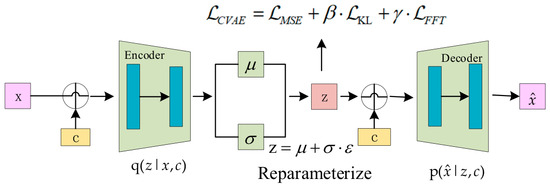
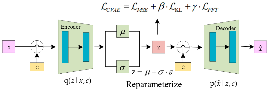
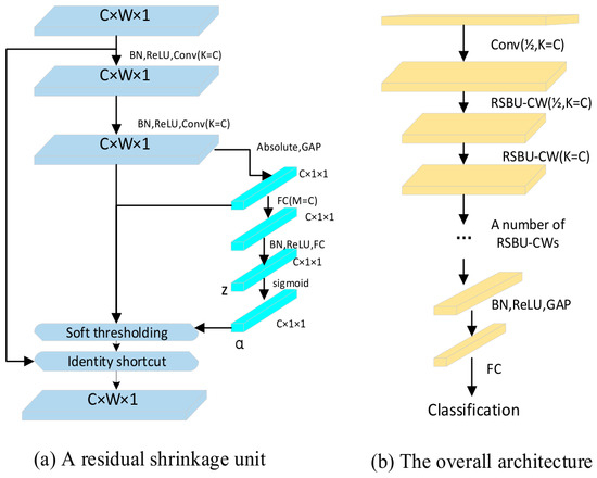
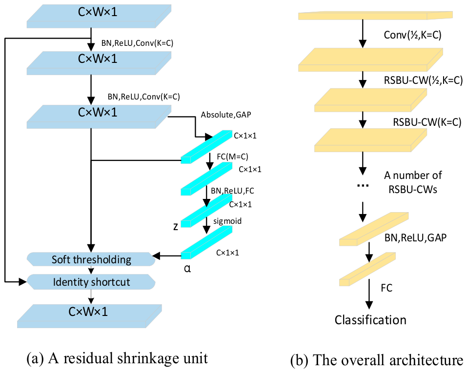
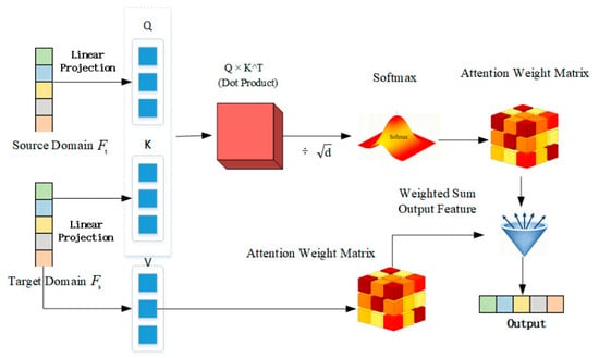
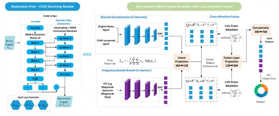
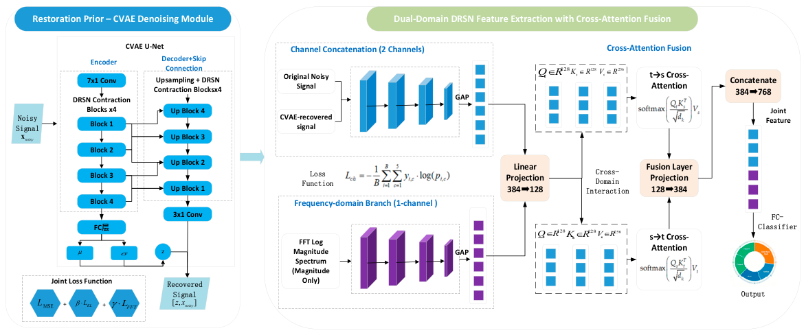
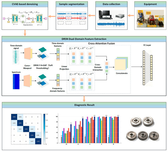
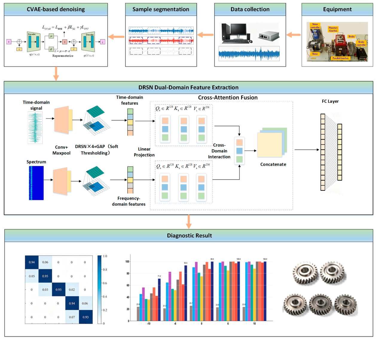
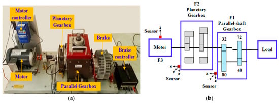
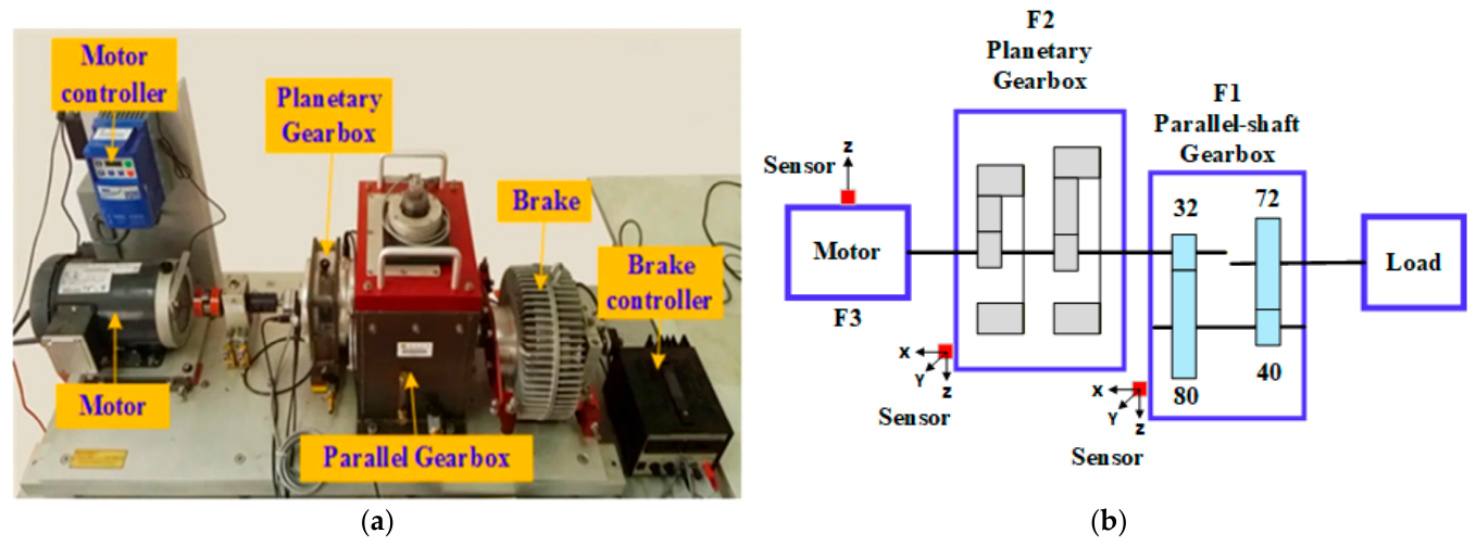
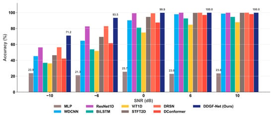
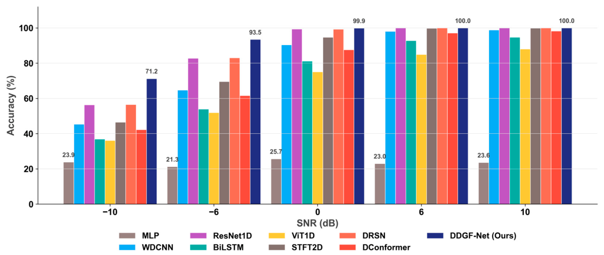
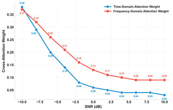
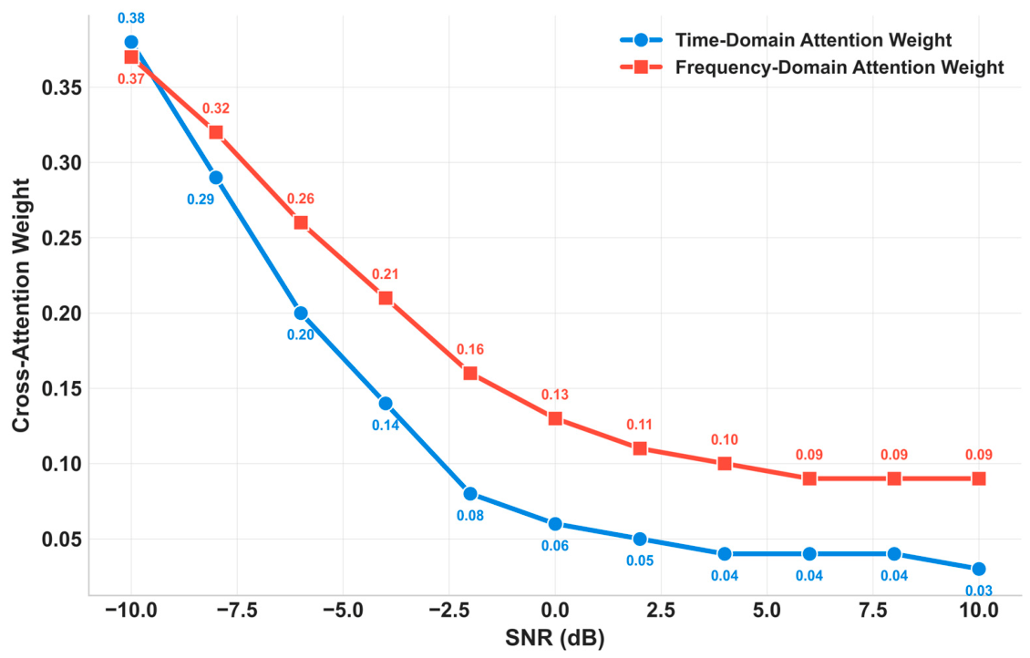
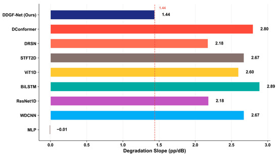
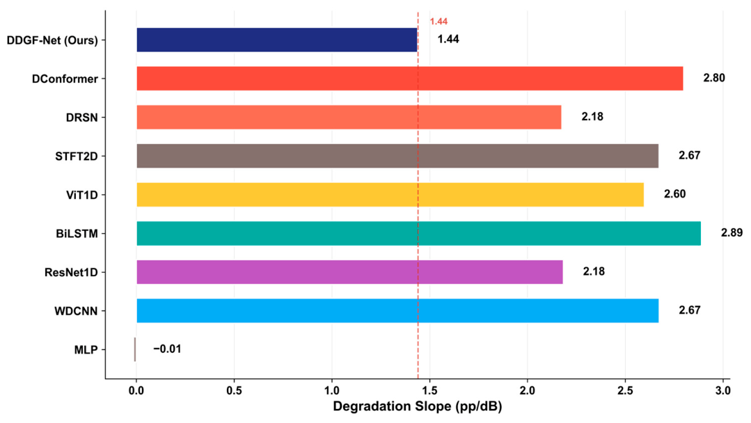
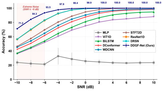
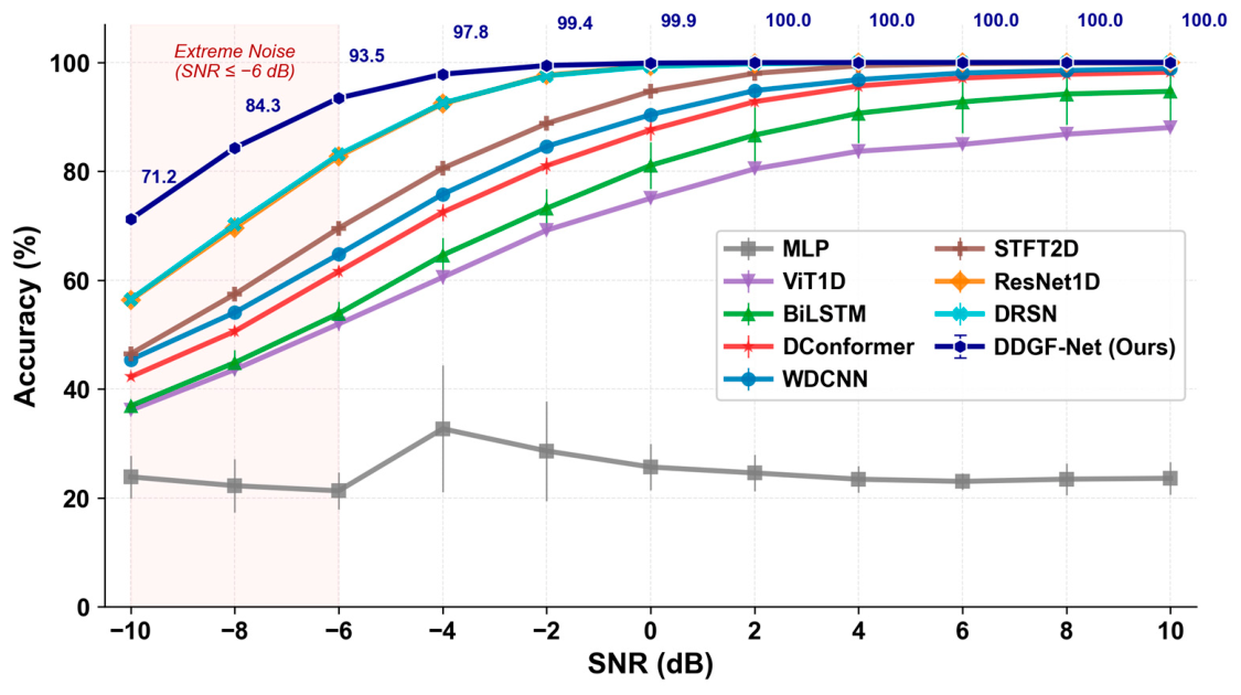
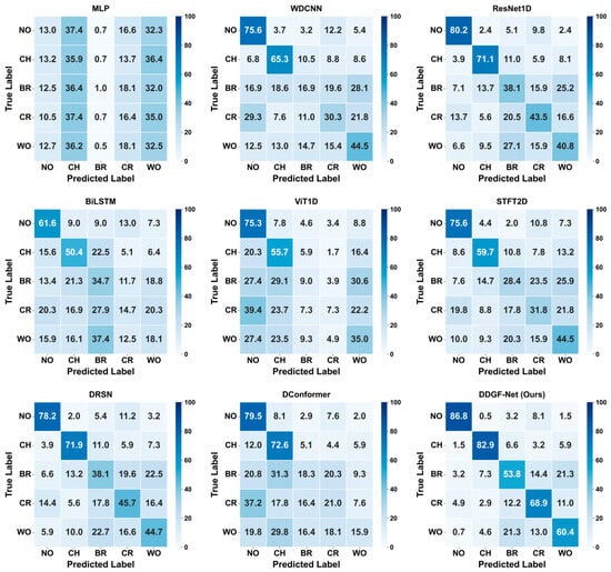
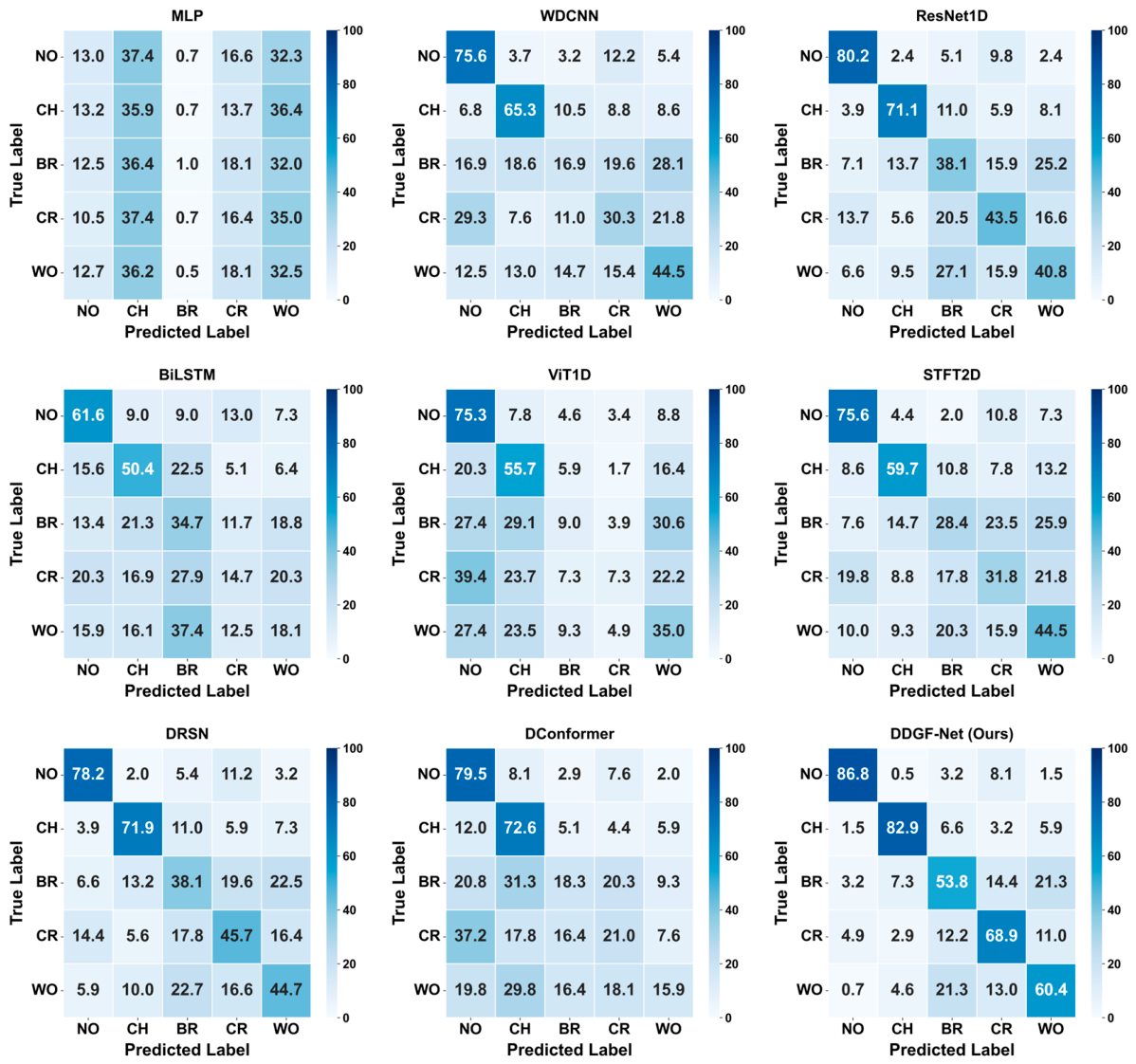
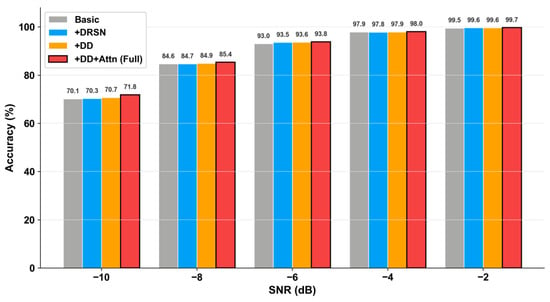
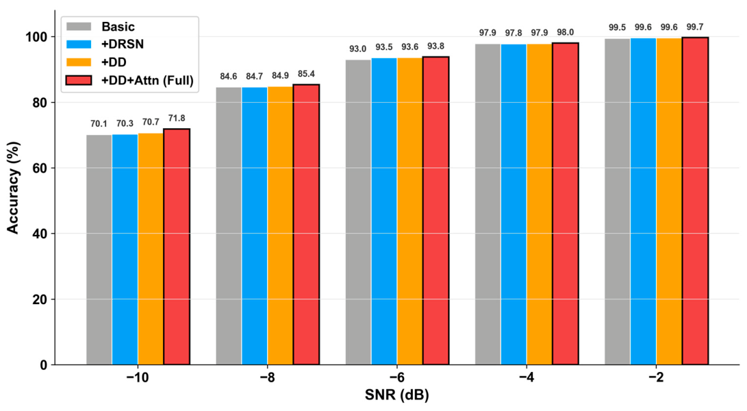
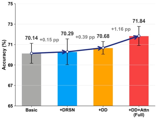
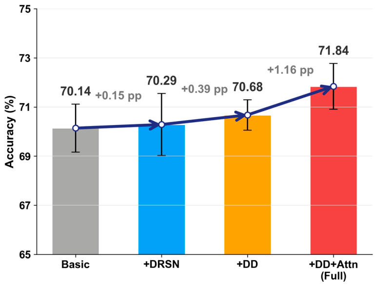

Disclaimer/Publisher’s Note: The statements, opinions and data contained in all publications are solely those of the individual author(s) and contributor(s) and not of MDPI and/or the editor(s). MDPI and/or the editor(s) disclaim responsibility for any injury to people or property resulting from any ideas, methods, instructions or products referred to in the content. |
© 2026 by the authors. Licensee MDPI, Basel, Switzerland. This article is an open access article distributed under the terms and conditions of the Creative Commons Attribution (CC BY) license.