


Abstract
Filtering-based stereo visual-inertial odometry often assigns fixed or uniformly scaled covariance to tracks accepted by the front-end, although accepted observations can differ in terms of tracking reliability, local directional identifiability, and agreement with the batch-level innovation model. This issue is important for UAV-based multisensor inspection platforms, where pose estimates support autonomous flight, measurement registration, repeatable survey lines, and multisensor data fusion. This paper presents RDIC-MSCKF, a Risk–Direction-Decoupled and Innovation-Calibrated MSCKF, where innovation calibration denotes bounded empirical scaling within the visual update. RDIC-MSCKF maps robust tracking diagnostics to a bounded standard-deviation multiplier and uses a robust local photometric information matrix to add penalty-only anisotropic covariance along weak image directions. The resulting observation covariance is preserved during MSCKF landmark elimination through full projected-covariance whitening. In parallel with feature-block innovation gating, bounded minimum measurement-noise inflation is estimated from the pre-gate innovation population and applied through a Kalman-equivalent modal update. On ten evaluated EuRoC MAV sequences, RDIC-MSCKF obtains lower ATE RMSE than the S-MSCKF baseline on nine sequences; averaged over five runs per sequence, the mean RMSE decreases from 0.1869 m to 0.1236 m, corresponding to a 33.8% reduction, and the sequence-mean P90 error decreases by 32.0%. Runtime profiling on five representative EuRoC sequences gives a 26.32 ms mean and 37.33 ms P95 per-frame processing time for RDIC-MSCKF, with 0.01% of profiled frames above the 50 ms reference. Outdoor UAV flights with RTK reference trajectories further demonstrate lower Sim(2)-aligned horizontal RMSE than S-MSCKF on all three evaluated flights.
1. Introduction
Visual-inertial odometry (VIO) fuses visual and inertial measurements to provide continuous six-degree-of-freedom state estimation when GNSS is unavailable or degraded, and has become a key localization technique for UAVs, mobile robots, and autonomous inspection platforms. UAV-based multisensor inspection platforms further require reliable onboard pose estimates for autonomous flight, multiscale measurement registration, repeatable survey trajectories, and multisensor data fusion. Related international studies on UAV surveying, UAV monitoring, and robot–environment interaction illustrate the broader demand for dependable perception and motion estimation in machine systems [1,2,3]. Existing VIO methods can be broadly divided into optimization-based and filtering-based approaches. Optimization-based methods typically employ sliding-window optimization, fixed-lag smoothing, factor-graph formulations, or IMU preintegration to jointly refine multiple states and visual constraints [4,5,6,7,8,9,10,11]. These methods often achieve high estimation accuracy at the cost of increased computation and memory, which is caused by window size, feature number, and repeated relinearization. Filtering-based VIO instead follows a recursive prediction–update structure and maintains only a bounded set of historical states, providing bounded-state dimension, stable memory usage, and predictable update latency. These properties remain attractive for online systems with limited computational resources.
The Multi-State Constraint Kalman Filter (MSCKF) is a representative filtering-based VIO framework [12]. It maintains the inertial state together with a finite number of cloned camera poses and eliminates landmark positions by projecting multi-view visual residuals onto the left nullspace of the landmark Jacobian. Stereo MSCKF further exploits left–right observations to strengthen scale constraints and feature initialization [13]. Its recursive structure also makes the visual-measurement model directly determine how much information enters the posterior state and covariance. Mismodeled visual uncertainty can, therefore, affect not only the current update but also subsequent recursive estimation.
Conventional MSCKF front-ends rely on KLT tracking, epipolar constraints, RANSAC, and innovation gating to reject inconsistent measurements. However, accepted observations do not necessarily have the same statistical precision. Motion blur, rapid motion, vibration, illumination variation, partial occlusion, repetitive texture, and stereo matching disturbances may degrade a feature before any hard rejection criterion is triggered. Front-end screening, therefore, determines whether a measurement is usable, whereas the filter update must further determine how much reliable information that measurement should contribute.
Recent navigation studies have also emphasized the importance of evaluating measurement reliability and sensing availability under degraded conditions. Self-evaluation and mutual-evaluation strategies have been investigated to quantify navigation sensor reliability in multi-source systems [14], while consistency checking and signal-quality weighting have been used to mitigate degraded GNSS measurements under NLOS and multipath conditions [15]. Forecasting external sensing degradation, such as satellite signal blockage, further highlights the value of anticipating unreliable measurements before severe degradation affects the navigation solution [16]. These studies provide broader context for reliability-aware navigation measurement processing. Nevertheless, for stereo visual-inertial odometry, an explicit measurement-level uncertainty path from visual observation reliability to covariance-consistent filtering updates remains insufficiently explored.
Adaptive measurement-noise estimation has, consequently, been introduced into MSCKF-based estimators. Variational-Bayesian approaches estimate time-varying observation noise online; Gaussian–generalized-inverse-Gaussian formulations model nonstationary visual-measurement noise; CAMSCKF represents different noise characteristics through multivariate parameter clustering; and innovation-based adaptive MSCKF methods regulate visual information using observed innovation statistics. These studies have advanced MSCKF from fixed covariance assumptions toward dynamic measurement-uncertainty modeling. Nevertheless, three issues remain in terms of the complete visual update chain.
First, visual uncertainty is both observation-dependent and direction-dependent. Tracking quality and stereo consistency determine the overall reliability of a feature, while local image structure determines its identifiability along different directions. Edge-like and weak-texture patches suffer from the aperture problem, producing markedly different information content along the gradient-normal and edge-tangent directions. The Lucas–Kanade normal matrix, Shi–Tomasi criterion, and related local structure measures expose this anisotropy [17,18,19]. Scalar covariance adaptation can change the overall weight of a measurement, but cannot explicitly represent such directional differences.
Second, once heteroscedastic and anisotropic covariance is introduced, its structure must be preserved through MSCKF landmark elimination. After left-nullspace projection, the observation covariance is generally transformed into a full feature-block covariance with non-diagonal correlations. Approximating it by a scalar or diagonal form can destroy part of the directional uncertainty modeled at the observation level. The covariance treatment must, therefore, remain consistent through landmark elimination and whitening.
Third, feature-level acceptance does not guarantee batch-level innovation consistency. Multiple features may be simultaneously affected by common motion, imaging conditions, or prior-state errors, causing the innovation population of the current update to deviate from its nominal scale. Estimating the measurement-noise scale only from post-gating low-residual measurements can further introduce truncation bias. Batch-level information, therefore, requires calibration based on the pre-gate innovation population.
These issues reveal a continuous uncertainty-propagation problem in MSCKF: observation reliability and directional identifiability shape the local covariance, landmark elimination transforms this covariance at the feature-block level, and the final update is further affected by the statistical scale of the innovation population. Existing adaptive MSCKF methods have addressed time-varying noise estimation, nonstationary covariance modeling, clustered uncertainty, and innovation-based adaptation, but the coupling among observation-wise risk–direction uncertainty, covariance-preserving nullspace projection, and pre-gate batch-innovation calibration has not been systematically treated within a unified update framework.
To address this problem, we propose RDIC-MSCKF, a Risk–Direction-Decoupled and Innovation-Calibrated MSCKF for stereo visual-inertial odometry. RDIC-MSCKF preserves the standard MSCKF inertial propagation, camera-state cloning, and bounded recursive structure, while introducing an uncertainty-processing chain from the observation level to the feature-block and batch levels. Tracking diagnostics and local photometric information separately characterize dynamic tracking risk and directional identifiability to construct heteroscedastic and anisotropic observation covariance. The full projected covariance is then preserved and whitened after landmark elimination, and a bounded measurement-noise inflation factor is estimated from the pre-gate innovation population to calibrate the information strength of the current visual batch.
The main contributions are summarized as follows:
- We develop a risk–direction-decoupled stereo visual-measurement-covariance model that separately captures observation-dependent tracking reliability and local directional identifiability, yielding heteroscedastic and anisotropic covariance for accepted visual measurements.
- We establish a covariance-preserving landmark-elimination and whitening formulation for anisotropic MSCKF measurements. The full covariance after nullspace projection is explicitly retained, and its equivalence to weighted nullspace processing is derived to preserve the statistical meaning of observation-level uncertainty through feature elimination.
- We introduce a bounded batch-innovation-calibration method based on the pre-gate innovation population. The method determines a minimum measurement-noise inflation factor to regulate batch-level visual information and employs a modal update algebraically equivalent to the corresponding inflated-noise Kalman update.
RDIC-MSCKF is evaluated using the EuRoC MAV benchmark and real-world UAV flight data. The evaluation considers trajectory accuracy, tail error, innovation statistics, finite-window update spectra, computational performance, and component-wise ablation to assess both estimation performance and the behavior of the proposed uncertainty-processing mechanisms.
2. Related Work
2.1. Filtering-Based VIO and Adaptive MSCKF
Filtering-based VIO performs recursive state estimation with bounded memory and computational cost. The original MSCKF removes landmark states through multi-view constraints and updates a finite set of cloned camera poses [12], while stereo extensions exploit synchronized left–right observations to strengthen scale constraints and feature initialization [13]. Subsequent filtering-based systems have incorporated online calibration [20], robocentric formulations [21], direct photometric residuals [22], and consistency treatments based on first-estimates Jacobians, observability analysis, and invariant error-state design [23,24,25]. OpenVINS provides a representative modern implementation of this class of estimators [26].
Measurement uncertainty has received increasing attention in MSCKF-based estimation. Variational-Bayesian S-MSCKF adapts observation-noise statistics online [27], while the Gaussian–generalized-inverse-Gaussian adaptive MSCKF models nonstationary visual-measurement noise [28]. CAMSCKF further distinguishes different time-varying noise characteristics through measurement clustering and covariance estimation [29]. More recent statistically adaptive MSCKF formulations use innovation statistics to regulate the visual update according to observed residual behavior [30]. These studies establish adaptive measurement uncertainty as an important extension of the standard MSCKF measurement model.
RDIC-MSCKF extends this line of research toward observation-wise structured uncertainty. Its measurement model separates tracking-related reliability from local directional identifiability, producing heteroscedastic and anisotropic covariance before landmark elimination. The resulting covariance structure is then retained through the projected MSCKF feature block and further regulated using batch-level innovation statistics.
2.2. Feature Reliability and Directional Visual Uncertainty
Visual front-ends commonly combine KLT tracking [17], Tomasi–Kanade or Shi–Tomasi feature scoring [18,31], stereo matching, epipolar checks, and RANSAC to select geometrically reliable correspondences. Forward–backward tracking, descriptor confidence, learned matching scores, and feature-budget policies provide additional measures of correspondence quality and computational control [32,33,34,35,36]. These mechanisms mainly determine whether a feature should be retained or rejected.
For retained measurements, local image structure also determines the direction in which image displacement can be reliably estimated. The Lucas–Kanade normal matrix and related structure-tensor formulations describe this local directional information [17,18,19]. Edge-like patches typically exhibit a strong and a weak eigen-direction, reflecting the classical aperture problem. Similar photometric information matrices are widely used in direct visual estimation [22,37].
This directional structure provides more information than a scalar feature score. In RDIC-MSCKF, tracking diagnostics describe the overall reliability of an accepted observation, whereas the local photometric information matrix determines its directional uncertainty. The two sources are combined in the measurement covariance rather than collapsed into a single scalar confidence.
2.3. Covariance Propagation and Innovation Adaptation
In standard MSCKF formulations with isotropic measurement noise, an orthonormal landmark-nullspace basis preserves the scalar covariance form after projection. Once observation-dependent anisotropic covariance is introduced, however, the projected covariance is generally full. The covariance introduced at the image level must, therefore, be retained through landmark elimination and whitening to preserve its directional information in the final update.
Innovation-based adaptive estimation provides a complementary mechanism for regulating the overall update strength. Classical covariance matching, NIS-based monitoring, probabilistic data association, and covariance inflation use residual statistics or association likelihoods to detect mismatch between the assumed and observed stochastic models [38,39,40,41,42]. Robust estimation and robust SLAM formulations also reduce the effect of outliers through loss functions, switchable constraints, dynamic covariance scaling, or bundle-adjustment robustification [43,44,45,46,47]. In visual-inertial estimation, related strategies have been used to adapt measurement uncertainty under changing sensing conditions [48].
RDIC-MSCKF combines these two levels of uncertainty treatment. Observation-dependent anisotropic covariance is propagated through the complete MSCKF feature block, while the pre-gate innovation population provides an additional bounded calibration of the current visual batch. This establishes a continuous covariance path from individual observations to landmark-eliminated constraints and, finally, to the batch-level Kalman update.
Table 1 shows the progression from global and cluster-wise covariance adaptation to finer-grained statistical treatment of visual measurements. RDIC-MSCKF focuses on the covariance path across three levels: observation-wise risk and directional uncertainty, covariance-preserving landmark elimination, and batch-level innovation calibration.
Table 1.
Comparison of representative adaptive MSCKF formulations.
3. Methodology
3.1. Problem Formulation and Method Overview
Let denote the MSCKF error state, which includes the IMU error variables and the active camera-clone pose errors. For feature j observed by clone i, the normalized stereo measurement is
Linearization gives
where is the landmark-position error. A single stereo observation is four-dimensional. The inertial propagation model, state augmentation, and observability treatment follow the standard MSCKF design and are not changed by the proposed visual-uncertainty model.
RDIC-MSCKF modifies the visual update through three estimator interfaces. At the observation level, tracking reliability and local image-direction information define an observation-dependent stereo covariance . At the feature-block level, this heteroscedastic and anisotropic covariance is carried through landmark elimination by retaining the full projected covariance before whitening. At the batch level, a bounded empirical inflation is applied to the accepted whitened system using statistics collected before feature-level truncation. These interfaces form one coupled update chain within the recursive MSCKF estimator.
The resulting visual-update procedure is summarized in Algorithm 1.
| Algorithm 1 Integrated RDIC-MSCKF Visual Update |
|
3.2. Risk–Direction Decoupled Observation Uncertainty
Dynamic tracking risk. For each accepted feature candidate in the current frame, the front-end provides diagnostic errors for left/right temporal tracking, left–right temporal imbalance, selective forward–backward disagreement, stereo epipolar consistency, disparity jump, and lifetime. The frame index is omitted in this paragraph for readability; the resulting metadata is stored per observation and is later used as , , and when feature tracks are stacked over clones. Let
collect the robustly normalized temporal mean, temporal imbalance, stereo epipolar, forward–backward, and disparity-jump diagnostics. Each entry is computed from the current candidate population by
where is the frame-level sample set for diagnostic family m, is a stability floor, and retains only above-median degradation. Forward–backward error is evaluated selectively for high-suspicion tracks under a computation budget. When the selective forward–backward check is not executed, its risk term is assigned the implementation-defined neutral value. No additional FB-based penalty is introduced, and the missing check is not interpreted as a measured zero-tracking error.
Figure 1 illustrates the corresponding information flow and uncertainty path.
Figure 1.
Integrated RDIC-MSCKF visual update chain. Stereo tracking produces visual observations and quality metadata. Tracking-risk and local photometric-information paths meet at the stereo observation covariance. Multi-view constraints are eliminated and whitened with the full projected covariance, after which the whitened blocks are split into accepted feature blocks and pre-gate batch statistics. The final update is performed by the bounded modal Kalman step. The left-to-right path shows how accepted stereo observations are converted into landmark-eliminated feature blocks, while the parallel uncertainty paths show how tracking reliability and directional image information define the covariance used before feature-level gating and batch-level calibration.
The tracking risk is represented as a quadratic robust energy
This energy is a monotone reliability score with design weights that encode the relative severity assigned to the diagnostic families. A lifetime tolerance
where denotes the current lifetime of track j. This factor prevents long-lived tracks from being penalized too aggressively for small transient deviations. The tracking quality and standard-deviation multiplier are
The multiplier acts on standard deviation; it enters covariance as . The back-end further clamps the received multiplier before squaring it, providing a bounded range for the covariance input.
Quality-aware feature management. The tracking quality forms the covariance multiplier and also regulates the visual constraint set before the back-end update. Within each image grid, features are ranked by a quality-aware score so that reliable and geometrically useful tracks are preferred when a cell contains more candidates than can be retained. Very low-quality tracks can be discarded even if they have not yet violated a hard geometric outlier test. Conversely, long-lived tracks with acceptable quality are allowed to survive grid competition because they provide multi-clone constraints and reduce unnecessary new feature initialization.
New feature detection follows the same quality-management policy. Grid cells with too few retained tracks are replenished by new detections, whereas cells already supported by high-quality tracks are not forced to add redundant features. When the total update row budget is approached, feature blocks are further ranked using projected information and innovation reliability so that the accepted stack remains computationally bounded. This policy controls the number, quality, and lifetime of feature blocks entering the MSCKF update, and, therefore, affects accuracy, finite-window spectra, and runtime.
Robust local photometric information. For a local patch expressed in the previous-image coordinates, let denote the tracked displacement from the previous image to the current image. The demeaned temporal photometric residual at pixel is
Assuming local photometric noise variance , the unweighted Gauss–Newton information for small image displacement is proportional to the sum of gradient outer products. With Huber weight
the robust observed-information approximation is
Because the Huber weights depend on observed residuals, is used as a weighted Gauss–Newton or robust observed-information matrix. Newly detected points use the current-image gradient version of the same approximation. The absolute photometric noise scale acts as a common proportional factor in the local information matrix. The subsequent covariance penalty uses relative eigenvalue ratios with respect to the frame reference, so the FIM path provides a relative directional-identifiability cue for the retained observation.
Let
The columns of are ordered by ascending eigenvalue, so is the weakly identifiable image direction and is the orthogonal strong direction in the pixel-gradient coordinate system. The sign of either eigenvector is immaterial because the covariance uses outer products. A small indicates aperture-like ambiguity. To avoid assigning super-baseline confidence to high-texture patches, the frame median
is computed from the valid local-information set and clipped to a positive implementation range. This value is used only as a relative penalty reference. The directional increments are
Thus,
Directional metadata is activated when the local information estimate passes reliability checks involving validity, track age, tracking quality, and stereo consistency.
Additive observation covariance. Let be the baseline normalized-plane measurement variance. The visual residuals used by the MSCKF update are defined in normalized image coordinates, while the local photometric directions are obtained from calibrated image patches. In general, a pixel-plane covariance for camera c is mapped to the normalized plane by the intrinsic Jacobian
For calibrated stereo cameras with near-square pixels, this diagonal normalization preserves local image directions to first order. The proposed covariance, therefore, uses the pixel-gradient eigenvectors as normalized-plane directional axes for the relative FIM penalty, while the baseline normalized variance sets the measurement scale. With this coordinate convention, the two-dimensional covariance assigned to one image observation is
where
The risk term expands the covariance isotropically according to dynamic reliability, whereas the photometric term adds direction-dependent variance associated with local identifiability loss. The design is additive rather than multiplicative, so the directional penalties are not scaled by tracking risk a second time. The stereo covariance uses the same two-dimensional block for the left and right observations,
This shared-quality construction applies the same calibrated directional covariance to the left and right observations, resulting in a block-diagonal stereo covariance.
Conservative properties. Because and ,
This establishes the risk covariance lower bound. In addition, Equations (15) and (18) imply that the photometric term can only preserve or increase covariance relative to the risk-only baseline. It, therefore, reduces visual information in weakly identifiable directions but never rewards a feature with below-baseline measurement noise.
The main symbols used in the formulation are summarized in Table 2.
Table 2.
Main symbols used in the non-experimental formulation.
The fixed parameter and implementation settings are listed in Table 3.
Table 3.
Fixed parameter and implementation settings used by the integrated RDIC-MSCKF configuration. All evaluated sequences use the same settings without sequence-specific tuning. Entries marked as implementation settings are fixed in the program but are not interpreted as statistically optimal constants.
3.3. Covariance-Preserving MSCKF Feature Elimination
For a feature observed in stereo frames, the residuals are stacked as
Here, , , and . Let and choose
with columns spanning the complete left nullspace of . The projected model is
Retaining as a full covariance is essential because a diagonal-only treatment would discard correlations introduced by projection. If is nonsingular, whitening gives
where .
Proposition 1.
Projection with complete covariance whitening is equivalent, up to a nonsingular basis change, to whitening the original feature model first and then applying a weighted landmark-nullspace projection.
Proof.
Define
Then,
and
Thus, is a whitened operator whose rows annihilate landmark uncertainty. If the original model is first whitened by , a weighted left-nullspace basis satisfies . Both and have dimension and span the complete row space of the landmark-eliminating whitened constraints. Hence, there exists a nonsingular matrix such that
When both whitened constraint bases are chosen orthonormally, is orthogonal. Under this orthogonal basis change, the state information matrix and information vector contributed by feature j are invariant:
For a nonsingular but non-orthogonal basis transformation, the same eliminated constraint space is represented with a correspondingly transformed covariance; the whitened orthonormal representation above is used to expose information equivalence. If is rank deficient, reduces the dimension of the eliminated landmark column space and increases accordingly; the same argument holds after a rank-revealing basis is used for . This linear-algebra statement does not require a degenerate feature to be accepted: the actual update still requires stable whitening of and subsequent innovation screening. If the numerical factorization of is ill-conditioned, eigenvalue whitening and diagonal whitening are stability fallbacks rather than the theoretical main path. □
3.4. Bounded Batch-Innovation Calibration
Each whitened feature block follows
With prior covariance , the nominal feature-block innovation covariance and normalized innovation statistic are
Feature-level chi-square gates reject clearly inconsistent feature blocks. A secondary normalized-statistic screen is used for conservative lost-feature updates. Batch calibration is estimated from the pre-gate population for which the feature-block statistic is computable, avoiding a batch scale estimated only from the low-residual subset that remains after gating.
Let
and define modal residual coordinates . If the whitened measurement noise is inflated from to , the feature statistic becomes
The eigenvalue represents the prior state uncertainty projected into innovation mode k, whereas is the observed innovation energy in that mode. The scalar inflates only the measurement-noise term after the observation-level covariance has been applied; it does not change the propagated state covariance.
Let be the batch quantile level, and let denote the median feature-block degrees of freedom, evaluated as the implementation’s integer median of block dimensions. The target normalized chi-square quantile is
Here, denotes the quantile of a chi-square distribution with degrees of freedom. The bounded minimum inflation problem is
For every feature block,
Therefore, is nonincreasing, and bisection finds the smallest feasible inflation in the configured interval up to the numerical search tolerance. If the number of computable feature blocks is below a threshold, calibration is not activated. If the quantile condition already holds at , no inflation is applied. If the upper bound cannot satisfy the condition, the bounded upper value is used. The calibration is empirical because feature blocks share the same state prior and may have different dimensions; the median degree of freedom provides a practical batch reference within the recursive visual update.
3.5. Modal Update, Properties, and Complexity
After feature-level screening, all accepted whitened constraints are stacked as
The standard Kalman form is
Let , , , and . Then, Equation (38) is equivalent to a unit-noise update defined by
Using the Woodbury identity and the thin SVD, the state correction is
The posterior covariance is
Equations (40) and (41) are obtained by diagonalizing through and are algebraically identical to the inflated-noise Kalman update for the same linearized system. Standard and numerical fallback update paths can use Joseph-form covariance updates, whereas the inflated path above uses an equivalent square-root modal information contraction.
Since ,
For a fixed prior, fixed linearization point, and identical accepted constraint set, the posterior information matrix with inflated noise is no larger than the nominal one. Hence,
For a fixed prior, linearization point, and accepted constraint set, this ordering states that batch inflation cannot increase visual-measurement information under the same linearized update model.
When the stacked whitened system has more rows than the state dimension, row compression is performed by QR factorization:
The residual term is independent of the state increment and can be omitted from the update. If a configured row budget is exceeded, accepted features are ranked by a score that increases with projected prior information and decreases with large normalized innovation. This ranking is a computational budget policy.
Table 4 summarizes the asymptotic cost of the main update operations.
Table 4.
Asymptotic cost of main update operations. N is the number of tracked candidates, B the selective forward–backward budget, L the number of pyramid levels, K the average KLT iterations, the patch area, the raw stacked stereo residual dimension of feature j, , the projected feature-block dimension, the number of batch-statistic blocks, the number of bisection iterations, M the accepted update rows, and the state dimension. Dense upper bounds are shown; practical MSCKF Jacobians retain clone sparsity and per-grid feature management is typically cheaper than global sorting.
4. Experiments
The experiments compare RDIC-MSCKF with a controlled S-MSCKF baseline under the same filtering structure, input data, calibration source, and evaluation protocol. The reported results characterize the final estimator configuration. The evaluation uses the public EuRoC MAV benchmark [49] to provide reproducible stereo visual-inertial sequences with industrial textures, illumination variation, and rapid motion. Additional real-world UAV flights provide platform-level validation of the spatial referencing capability required by UAV-based multisensor inspection platforms.
The controlled comparison keeps the underlying MSCKF state, IMU propagation, cloning, camera–IMU calibration source, EuRoC stereo/IMU streams, trajectory intervals, state-window settings, and evaluation scripts fixed for S-MSCKF and RDIC-MSCKF. Unless otherwise stated, trajectory errors are computed after rigid SE(3) fixed-scale alignment, and repeated runs are summarized at the sequence level. ROVIO and VINS-Mono are included as same-platform reference results because their front-ends and estimator architectures differ from those of the controlled S-MSCKF comparison. The runtime environment and timing scope are summarized in Table 5.
Table 5.
Runtime profiling environment and timing scope.
4.1. EuRoC Accuracy Comparison
Table 6 reports the EuRoC benchmark ATE statistics. The S-MSCKF and RDIC-MSCKF entries are computed from repeated-run APE summaries under the baseline and RDIC configurations, respectively.
Table 6.
ATE statistics on the EuRoC dataset (meters), reported as RMSE/STD/P90.
The EuRoC sequences provide complementary accuracy conditions. The machine-hall sequences include larger spatial motion, industrial texture, illumination variation, and longer trajectories, which tend to expose errors associated with marginal feature tracks and heterogeneous measurement quality. The Vicon-room sequences are shorter and are captured in a more controlled indoor environment, but they still contain fast motion, viewpoint changes, and texture-dependent tracking difficulty. V2_03 is excluded because both filtering configurations failed to complete the sequence after persistent stereo-matching loss associated with severe left–right photometric inconsistency.
For RDIC-MSCKF and S-MSCKF, each RMSE, STD, and P90 entry is the arithmetic mean of the corresponding APE-summary metric over five repeated runs for that sequence. RMSE measures the average aligned trajectory error, the APE-summary STD measures dispersion of the aligned position error within the trajectory summaries, and P90 reflects the upper tail while being less sensitive than the maximum to rare events. This table statistic is distinct from the run-to-run standard deviation shown as error bars in Figure 2. The sequence-mean values quoted in the Abstract and Conclusions are computed from the same sequence-level arithmetic means.
Figure 2.
EuRoC ATE-RMSE comparison between S-MSCKF and RDIC-MSCKF. Bars show the mean over five repeated runs for each sequence, and error bars show run-to-run standard deviation.
Table 6 shows that RDIC-MSCKF improves over the S-MSCKF baseline on most EuRoC sequences. The difference is especially clear in the machine-hall group, where RDIC-MSCKF reduces all three reported ATE statistics on MH_01–MH_04 and reduces RMSE on MH_05.
RDIC-MSCKF reduces RMSE on V1_01, V1_02, V1_03, and V2_02, whereas S-MSCKF remains better on V2_01. These results indicate that the benefit depends on sequence conditions. Covariance-aware information scaling is most useful when accepted visual measurements exhibit substantial covariance mismatch; on well-conditioned sequences, reduced visual information can slightly degrade accuracy. ROVIO and VINS-Mono provide architectural context, whereas the controlled comparison is between RDIC-MSCKF and S-MSCKF.
Figure 2 provides a sequence-wise visual summary of the repeated-run RMSE values for the two filtering variants. It complements Table 6 by showing whether the numerical differences are consistent across runs. Figure 3 gives a representative MH_02 trajectory-level comparison against ground truth and same-platform VIO references. The trajectory plot uses clearly separated trajectory lines to illustrate the path differences corresponding to the reported ATE values.
Figure 3.
Trajectory comparison on the EuRoC MH_02 sequence.
4.2. Contextual Comparison with Adaptive MSCKF Methods
To place the improvement of RDIC-MSCKF in the context of recent adaptive MSCKF studies, we further compare the relative accuracy gains reported by representative methods with respect to their own MSCKF baselines. Direct comparison of absolute trajectory errors across different publications is not appropriate because the implementations, parameter settings, sequence subsets, initialization procedures, and evaluation protocols are not identical. We, therefore, use the within-study relative reduction
where and denote the sequence-averaged position error reported for the baseline and the corresponding adaptive method, respectively.
Table 7 summarizes the results calculated from the numerical values reported in the original publications. VBU-SMSCKF [27] reduces the mean EuRoC RMSE from 0.1946 m to 0.1261 m over eight reported sequences, corresponding to a 35.2% reduction. The ANGIG-KF2 formulation [28] reduces the reported mean APE from 0.170 m to 0.120 m over eleven EuRoC sequences, corresponding to a 29.4% reduction. QA-MSCKF [30] reduces the mean RMSE from 0.278 m to 0.185 m over ten reported EuRoC sequences, giving a 33.5% reduction. Under the controlled evaluation protocol of the present study, RDIC-MSCKF reduces the sequence-average RMSE from 0.1869 m to 0.1236 m, corresponding to a 33.8% reduction.
Table 7.
Within-study position-error reductions in representative adaptive MSCKF methods on EuRoC. Literature values were calculated from the numerical results reported in the corresponding publications.
The within-study reductions show that adaptive measurement-uncertainty treatment produces substantial gains across different MSCKF formulations, with reported position-error reductions of approximately 29–35%. RDIC-MSCKF achieves an improvement of comparable magnitude while using a different uncertainty model: tracking-related reliability and local directional identifiability are represented at the observation level, the resulting anisotropic covariance is preserved through landmark elimination, and the remaining batch-level innovation mismatch is subsequently calibrated.
The sequence-wise behavior also provides useful context. VBU-SMSCKF improves all eight EuRoC sequences reported in its original comparison, ANGIG-KF2 reduces the reported APE on ten of eleven sequences, and QA-MSCKF improves RMSE on six of ten sequences. In the present controlled evaluation, RDIC-MSCKF improves RMSE on nine of the ten successfully evaluated EuRoC sequences. These results indicate that the proposed method achieves a within-study gain of comparable magnitude while maintaining relatively broad improvement across the evaluated sequences.
4.3. Component-Wise Ablation Study
To examine the cumulative effect of the proposed mechanisms, we conduct an ablation study on the ten successfully evaluated EuRoC sequences. All configurations use the same S-MSCKF state definition, inertial propagation, camera cloning, sensor calibration, and evaluation protocol. Starting from the S-MSCKF baseline A0, the proposed mechanisms are introduced sequentially along the uncertainty-processing chain, as summarized in Table 8.
Table 8.
Configurations used in the component-wise ablation study.
A1 introduces observation-dependent tracking-risk covariance. A2 further incorporates directional covariance derived from local photometric information. A3 preserves the full projected covariance after landmark nullspace elimination, allowing the anisotropic observation uncertainty introduced in A2 to remain represented at the feature-block level. Finally, A4 introduces bounded batch-innovation calibration together with quality-aware feature management and corresponds to the complete RDIC-MSCKF configuration.
Table 9 reports the ATE-RMSE of A0–A4. The sequence-average RMSE decreases from 0.1869 m for the S-MSCKF baseline to 0.1236 m for the complete RDIC-MSCKF, corresponding to an overall reduction of 33.8%. The intermediate configurations show that the improvement arises progressively from observation-level uncertainty modeling, covariance propagation, and batch-level calibration.
Table 9.
Component-wise ablation results on EuRoC. ATE-RMSE is reported in meters.
The largest incremental gain is obtained in A1. Introducing tracking-risk covariance reduces the average RMSE from 0.1869 m to 0.1531 m and improves all ten evaluated sequences. This result indicates that feature tracks retained by the standard front-end still exhibit substantial observation-to-observation differences in measurement reliability. Modeling this variability directly in the measurement covariance, therefore, provides a strong correction to the fixed-noise assumption.
A2 further introduces directional uncertainty derived from local photometric information. The average RMSE decreases to 0.1472 m. Its effect is sequence dependent; for example, MH_03 improves from 0.231 m to 0.173 m, whereas several other sequences change only slightly. This behavior is consistent with the directional model, whose influence becomes more pronounced when accepted image patches contain weakly constrained directions. The result shows that observation-dependent scalar scaling alone does not capture all of the uncertainty structure present in visual measurements.
A3 preserves the full covariance generated after landmark nullspace projection. The average RMSE decreases from 0.1472 m to 0.1297 m. Pronounced gains are observed on MH_01, MH_02, MH_04, and V2_02; on MH_02; for example, the RMSE decreases from 0.144 m to 0.072 m. These results demonstrate that once anisotropic observation covariance is introduced, its projected correlation structure can materially affect the information carried by an MSCKF feature block. Preserving and whitening the full projected covariance is, therefore, important for propagating observation-level uncertainty through landmark elimination.
A4 adds the bounded batch-innovation calibration together with quality-aware feature management. The sequence-average RMSE is further reduced to 0.1236 m, with clear improvements on MH_02, MH_03, V1_01, V1_02, and V1_03. This final-stage gain reflects the combined effect of update-level innovation regulation and quality-aware control of the retained visual-constraint population. Because these mechanisms are activated jointly in A4, their individual contributions are not separated in this cumulative ablation.
Tail-Error Behavior
In addition to the average trajectory error, we evaluate the P90 error to examine the upper-tail behavior across the cumulative configurations of the trajectory-error distribution. Table 10 summarizes the sequence-average ATE-RMSE and P90 statistics for A0–A4.
Table 10.
Aggregate accuracy and tail-error statistics of the ablation configurations.
The P90 results follow the same overall trend as the average trajectory error. Introducing tracking-risk covariance in A1 reduces the mean P90 from 0.272 m to 0.226 m, corresponding to a 16.9% reduction relative to A0. This result indicates that observation-dependent reliability modeling suppresses a substantial portion of the large-error population in addition to improving the average trajectory accuracy.
Directional covariance in A2 further reduces the mean P90 to 0.218 m, giving a cumulative reduction of 19.9%. The additional improvement is moderate, consistent with the structure-dependent nature of directional uncertainty: its effect is concentrated in observations whose local image geometry contains weakly constrained directions.
Preserving the full projected covariance in A3 produces a more pronounced reduction in the upper error tail, decreasing the mean P90 to 0.193 m, or 29.0% below the baseline. Together with the corresponding RMSE reduction, this result indicates that retaining the correlation structure generated by anisotropic observations after landmark elimination affects both the typical trajectory error and its upper tail.
The complete RDIC-MSCKF configuration A4 achieves the lowest mean P90 of 0.185 m, corresponding to an overall reduction of 32.0% relative to A0. The smaller incremental change from A3 to A4 is consistent with the combined role of bounded batch calibration and quality-aware management: they regulate the update scale and retained visual-constraint population rather than uniformly modifying every visual update.
Overall, the RMSE and P90 results exhibit consistent cumulative trends. Tracking-risk covariance provides the largest initial gain, directional covariance offers structure-dependent refinement, full projected-covariance preservation substantially reduces both average and tail errors, and the complete A4 configuration provides the final bounded correction at the update level. The following NIS and NEES analyses further examine how these components affect the statistical behavior of the accepted visual updates.
4.4. Real-World UAV Trajectory Evaluation
To complement the public benchmark, we further evaluate the three VIO configurations on real-world UAV flights collected by the experimental platform shown in Figure 4. The flights provide an outdoor platform-level evaluation of stereo visual-inertial trajectory estimation under illumination variation, airframe vibration, and six-degree-of-freedom motion. The platform is equipped with a forward-facing Intel RealSense D435i stereo camera rigidly mounted on the airframe, and the D435i internal IMU provides the inertial measurements. The stereo image stream is recorded at a resolution of pixels and a frame rate of 20 Hz, while the IMU is recorded at 200 Hz. An RTK trajectory is recorded as the external reference for horizontal trajectory evaluation after Sim(2) alignment.
Figure 4.
Real-world UAV platform used for the flight experiments. The platform carries a forward-facing Intel RealSense D435i stereo camera with its internal IMU; the recorded stereo image resolution is pixels at 20 Hz and the IMU rate is 200 Hz.
The onboard stereo-inertial data are processed by S-MSCKF, RDIC-MSCKF, and VINS-Mono, and the corresponding RTK trajectory is used as the horizontal reference. The RTK latitude, longitude, and altitude measurements are converted to a local ENU frame with the first valid RTK sample as the origin. For trajectory visualization and horizontal error reporting, each estimated trajectory is time-associated with the RTK sequence and aligned to the RTK ENU-XY path by a planar similarity transformation. Because Sim(2) alignment removes planar translation, heading, and scale, these metrics evaluate horizontal path shape rather than metric-scale accuracy.
Figure 5 and Table 11 show that the Sim(2)-aligned RDIC-MSCKF trajectories have smaller aligned horizontal path errors than the S-MSCKF baseline in all three flights. The aligned horizontal RMSE values of RDIC-MSCKF are 3.89 m, 8.34 m, and 2.87 m on UAV-1–UAV-3, respectively, whereas S-MSCKF obtains 17.80 m, 17.76 m, and 3.51 m. VINS-Mono provides an additional architectural reference with RMSE values of 10.53 m, 8.25 m, and 5.43 m. The second flight shows comparable RDIC-MSCKF and VINS-Mono aligned horizontal path error, while the first and third flights show clearer separation between RDIC-MSCKF and the reference methods. The UAV flights, therefore, provide additional outdoor evidence under illumination variation, airframe vibration, and six-degree-of-freedom platform motion.
Figure 5.
Real-world UAV trajectory comparison on three flight sequences. The panels labeled UAV-1, UAV-2, and UAV-3 correspond to three UAV runs with RTK reference trajectories.
Table 11.
Horizontal trajectory errors after Sim(2) alignment to the RTK reference (meters), reported as RMSE/Mean/P90 after time association and planar similarity alignment to the RTK ENU-XY reference.
4.5. Finite-Window Update-Spectrum Diagnostics
To examine how retained visual updates affect the numerical geometry of the filtered update, we evaluate finite-window effective-Jacobian spectra on five representative EuRoC sequences: MH_03, MH_04, MH_05, V1_02, and V1_03. This analysis complements ATE by characterizing the spectral structure of the constraints entering the bounded-state filter.
Following the source-resolved diagnostic protocol, visual updates are separated into remove updates formed by terminated feature tracks and prune updates triggered by camera-state sliding-window management. The diagnostic matrix is the effective whitened update Jacobian for the current finite camera-clone window, whose logged window size reaches 20 camera states in prune updates. Let its retained singular values be after the diagnostic logger removes numerically ineffective values, with r recorded as ‘full_rank_count’. We define
where M is the number of update rows and is the active error-state dimension. The condition-number diagnostic is
using the minimum retained singular value reported by the same logger. Higher normalized effective rank and lower indicate a more balanced numerical update spectrum. The violin plots use sequence-balanced frame-level samples. For each method, source, metric, and sequence, 500 samples are drawn with a fixed random seed, using subsampling when more samples are available and sampling with replacement when fewer samples are available. The plotted summaries avoid domination by longer sequences; the equal-sequence median values reported below average the per-sequence medians over the five evaluated sequences.
Figure 6 shows that the two update sources behave differently. For remove updates, RDIC-MSCKF decreases the equal-sequence median normalized effective rank from 0.2393 to 0.1942 and increases the median condition number from 4.1692 to 4.6372, indicating a less balanced spectrum. For prune updates, the normalized effective rank is nearly unchanged, moving from 0.01948 to 0.01973, while the lower condition number, 4.3176 versus 4.7569, indicates improved spectral balance. These finite-window spectra characterize the numerical geometry of accepted update blocks.
Figure 6.
Source-resolved finite-window update-spectrum diagnostics for S-MSCKF and RDIC-MSCKF on MH_03, MH_04, MH_05, V1_02, and V1_03. Violin shapes show sequence-balanced frame-level distributions; thick and thin vertical segments denote interquartile and 10th–90th percentile ranges, respectively, and white markers denote medians. The upper row reports normalized effective rank, and the lower row reports condition number.
4.6. Consistency and Numerical Behavior
4.6.1. Innovation and Covariance Diagnostics
To examine how the proposed components affect the statistical behavior of the visual update, we evaluate A0–A4 on five representative EuRoC sequences: MH_03, MH_04, MH_05, V1_02, and V1_03. Here, A0 denotes the standard S-MSCKF baseline; A1 introduces tracking-risk covariance; A2 further incorporates directional covariance; A3 retains the full projected covariance after landmark elimination; and A4 corresponds to the complete RDIC-MSCKF with bounded batch-innovation calibration and quality-aware feature management.
For each accepted visual update, the normalized innovation squared (NIS) is computed as
where , , , and denote the stacked innovation, measurement Jacobian, prior covariance, and measurement covariance used in the corresponding update. Since the dimension of the stacked visual constraint varies with the number of retained feature blocks, the 95% NIS confidence bound is evaluated using the actual update dimension at each frame. The reported NIS statistics are computed from accepted updates and are, therefore, used as diagnostics of the innovation scale admitted by the filter.
To further examine the relationship between estimated uncertainty and translational error, we report an aligned position block-NEES,
where is the position error after applying the rigid transformation used for ATE evaluation, and is the corresponding aligned position covariance block. Given the alignment rotation ,
Because the alignment is estimated from the complete trajectory, this quantity is used as a translational covariance diagnostic rather than a strict online full-state NEES test.
For the position block-NEES, we report the median normalized by its dimension, the ratio between its 90th percentile and the 95% bound, and the fraction of samples lying within the corresponding 95% confidence region. A normalized median near one indicates agreement between the typical translational error scale and the estimated covariance scale. Values substantially below one indicate conservative covariance, whereas large upper-tail ratios indicate episodes in which the estimated covariance is small relative to the observed error.
Table 12 reveals a clear change in the accuracy–uncertainty relationship across the ablation sequence. The S-MSCKF baseline A0 achieves an inside95 ratio of 0.948 for the aligned position block, but its normalized median NEES is only 0.075. Its NIS P90/dim is likewise very small at 0.007. Together with an ATE-RMSE of 0.2406 m, these statistics indicate a strongly conservative covariance scale in the evaluated translational subspace.
Table 12.
Accuracy and consistency-oriented diagnostics for five representative EuRoC sequences.
Introducing tracking-risk covariance in A1 reduces the ATE-RMSE from 0.2406 m to 0.1946 m. The normalized median position NEES increases to 2.284, showing that observation-dependent reliability modeling substantially changes the information assigned to accepted visual measurements. The accompanying increase in the upper NEES tail indicates that tracking-risk adaptation alone does not fully regulate the covariance behavior of difficult visual updates.
Directional covariance is introduced in A2 to account for local weak and strong image directions. The ATE-RMSE is further reduced to 0.1840 m and the normalized median position NEES decreases from 2.284 to 1.464. The P90 NEES ratio, however, remains large, indicating that directional uncertainty improves the typical covariance scale but does not by itself suppress all high-error tail events.
A3 retains the full feature-block covariance after landmark nullspace projection. This reduces the ATE-RMSE to 0.1782 m and lowers the normalized median position NEES to 1.176. More importantly, the P90 NEES ratio decreases from 28.804 for A2 to 6.666 for A3. The result indicates that preserving the covariance structure generated by anisotropic observations through landmark elimination improves the relationship between observation-level uncertainty modeling and the final MSCKF update.
The complete RDIC-MSCKF configuration A4 further introduces bounded batch-innovation calibration and quality-aware feature management. It achieves the lowest ATE-RMSE of 0.1664 m and a normalized median position NEES of 0.864, which is the closest to unity among the evaluated variants. The P90 NEES ratio is further reduced to 4.046. Although the position inside95 ratio of 0.768 remains below the nominal 95% level, the combined results show a substantially improved tradeoff between trajectory accuracy, typical covariance scale, and high-NEES tail behavior.
The NIS statistics provide a complementary view. A0 exhibits an extremely small normalized innovation scale, consistent with its conservative covariance behavior. A1 and A2 substantially increase the innovation scale as more informative observation-dependent covariance models are introduced. A3 and A4 moderately reduce the NIS upper-tail level while retaining much higher normalized innovation values than A0. Thus, the accuracy improvement of RDIC-MSCKF is not obtained by simply increasing the aggressiveness of the visual update; the later stages of the covariance-processing chain regulate the information introduced by the earlier observation-level adaptations.
Figure 7 further shows that the effects vary across sequences, with the complete RDIC-MSCKF generally reducing excessive position-NEES events while maintaining lower trajectory error. These results support the complementary roles of the proposed components: tracking-risk covariance adapts observation-level reliability, directional covariance captures local anisotropy, full projected covariance preserves this uncertainty through landmark elimination, and batch-innovation calibration regulates the remaining update-level mismatch.
Figure 7.
Per-sequence innovation and covariance diagnostics for A0–A4 on representative EuRoC sequences. Each heatmap reports the raw statistic indicated by its color bar. The progression from A0 to RDIC-MSCKF illustrates how observation-level uncertainty modeling, projected-covariance preservation, and batch calibration affect the accuracy–uncertainty relationship of the filter.
The reported quantities should be interpreted as consistency-oriented diagnostics rather than a proof of full-state statistical consistency. In particular, the position block-NEES depends on trajectory alignment, while the NIS statistics are conditioned on accepted visual updates.
4.6.2. Representative Update-Level NIS Behavior
The preceding multi-sequence analysis summarizes the overall innovation and covariance behavior of A0–A4. To further examine how the innovation scale evolves during individual visual updates, we use the EuRoC MH_02 sequence as a representative case and compare the update-level NIS/DoF trajectories of S-MSCKF and RDIC-MSCKF.
For each accepted visual update, the NIS is computed according to Equation (48). Because the residual dimension varies with the number of retained constraints, we report the normalized quantity
where denotes the dimension of the visual residual represented by the corresponding update log after landmark elimination, covariance whitening, feature-level gating, and row compression. The normalized NIS provides a dimension-independent indicator of the innovation scale admitted by each accepted update. Under an ideal locally linearized model with correctly specified innovation covariance, its expected scale is approximately one.
Figure 8 shows the raw update-level NIS/DoF values and their moving averages on MH_02. A moving-average window of 25 accepted updates is used to reveal the temporal trend, while the dashed horizontal line at indicates the nominal reference scale.
Figure 8.
Representative update-level NIS/DoF behavior on EuRoC MH_02. Raw accepted-update statistics and their 25-update moving averages are shown for S-MSCKF and RDIC-MSCKF. The dashed line denotes the nominal reference .
The S-MSCKF moving average remains below the unit reference for most of the sequence, consistent with the conservative innovation scale observed in the multi-sequence statistics. RDIC-MSCKF shifts the accepted-update NIS/DoF toward the nominal range over substantial portions of the trajectory, while retaining transient excursions in several intervals. These excursions indicate that the proposed uncertainty treatment does not force the innovation statistic toward a fixed target on every update; instead, the resulting scale reflects the interaction among observation-dependent covariance, projected feature-block covariance, and batch-level calibration.
This temporal behavior complements the aggregate results in Table 12. The baseline exhibits low normalized innovation values together with relatively large trajectory error, whereas RDIC-MSCKF admits a less conservative innovation scale while achieving lower ATE. The bounded batch calibration subsequently limits excessive visual information when the pre-gate innovation population indicates a batch-level scale mismatch.
The NIS/DoF curves should be interpreted as diagnostics of the accepted visual-update population rather than as a standalone proof of full filter consistency. In particular, the plotted statistics are conditioned on feature-level gating and other front-end selection operations.
4.7. Computational Efficiency Analysis
Runtime feasibility is essential for a filtering-based stereo VIO system because the estimator must process each stereo frame while maintaining bounded latency for downstream control and navigation. The runtime comparison on the same platform includes the added uncertainty calculations, quality-aware feature management, and covariance-aware update.
Runtime profiling is performed on five representative EuRoC sequences: MH_02, MH_03, MH_05, V1_02, and V1_03. The first 10 s of each sequence are excluded to reduce initialization and cache-warm-up effects. Front-end and back-end timing records are associated by nearest timestamps within a 12-ms tolerance. For each profiled stereo frame, the per-frame processing time is defined as the sum of the measured front-end and back-end processing times. This definition measures estimator processing demand; rosbag playback, ROS transport latency, and offline trajectory evaluation are excluded. Since EuRoC stereo images are provided at 20 Hz, 50 ms is used as the nominal per-frame processing reference. Aggregate statistics are first computed per sequence and then equally averaged over the five sequences.
Figure 9 shows the net cost of the two configurations. In the back-end, RDIC-MSCKF is slower than S-MSCKF, which is consistent with the additional covariance construction, projected whitening, feature-block statistic evaluation, and bounded batch calibration. In the front-end, RDIC-MSCKF is faster in the plotted sequences because quality-aware feature management changes the number, lifetime, and replenishment pattern of retained visual constraints.
Figure 9.
Runtime breakdown of S-MSCKF and RDIC-MSCKF. Blue denotes S-MSCKF and red denotes RDIC-MSCKF. The reported timing includes both uncertainty calculations and changes in the retained visual-constraint population.
Table 13 summarizes the corresponding equal-sequence averages. The mean per-frame processing time decreases from 36.77 ms for S-MSCKF to 26.32 ms for RDIC-MSCKF, and the P95 value decreases from 61.69 ms to 37.33 ms. The front-end accounts for most of the reduction, decreasing from 30.24 ms to 18.56 ms on average, whereas the back-end mean increases from 6.44 ms to 7.76 ms. The lower total runtime reflects the combined effect of additional back-end computation and a reduced front-end feature-processing load.
Table 13.
Equal-sequence average runtime statistics for five representative EuRoC sequences.
Figure 10 further reports the frame-by-frame timing behavior. The yellow dashed line provides a 50 ms reference corresponding to a 20 Hz stereo-frame budget. Faint curves show individual-frame measurements, which can contain occasional spikes, and solid curves show moving-average trends. The RDIC-MSCKF moving-average curves remain below the 50 ms reference on the plotted sequences, and Table 13 reports a 26.32 ms mean, a 37.33 ms P95, and 0.01% of profiled frames exceeding 50 ms. These statistics support real-time compatibility on the evaluated platform while still allowing isolated raw-frame spikes.
Figure 10.
Per-frame processing time of S-MSCKF and RDIC-MSCKF. Blue denotes S-MSCKF, red denotes RDIC-MSCKF, and the yellow dashed line marks the 50 ms reference budget.
5. Discussion
5.1. Interpretation of the Integrated Uncertainty Model
RDIC-MSCKF treats accepted stereo tracks as a heterogeneous measurement set. Tracking diagnostics describe dynamic and matching reliability, including motion blur, illumination variation, partial occlusion, stereo imbalance, and disparity discontinuities. Local photometric information describes directional identifiability, especially near edges and weak-gradient regions where the aperture problem makes two-dimensional localization anisotropic. Batch calibration then acts after landmark elimination and whitening, where the relevant question is whether the current population of feature-block innovations is compatible with the assumed visual update model. These three levels address different sources of uncertainty while preserving the MSCKF propagation, cloning, and landmark-elimination structure.
Hard gates and RANSAC-type tests remain necessary for clearly inconsistent feature blocks. RDIC-MSCKF adds a covariance path for measurements that pass these tests but still differ in terms of reliability or directional precision. This differs from residual-only robust losses: tracking and photometric diagnostics are formed before the final Kalman update and are explicitly carried through the covariance algebra.
5.2. Accuracy and Information Scaling
The penalty-only FIM mapping keeps high-texture patches at the baseline noise level unless additional calibration evidence is available. This reduces the risk of overconfident visual updates, while also attenuating some useful constraints in favorable scenes. The V2_01 result is consistent with this trade-off: S-MSCKF remains slightly better when the fixed-covariance baseline is already well matched to the sequence conditions.
The bounded batch inflation has a related effect. Because , the batch step reduces or preserves visual information for a fixed prior, linearization point, and accepted constraint set. Consequently, the method may reduce update strength when elevated batch statistics arise from prior mismatch or correlated observations rather than measurement noise alone.
5.3. Computational Behavior
The runtime results show a redistribution of computation. RDIC-MSCKF adds back-end operations for covariance construction, projected whitening, feature-block statistics, and modal updating. At the same time, quality-aware feature management changes the retained track population and reduces the front-end feature-processing load in the profiled sequences. The measured per-frame processing time, therefore, reflects both effects: a higher back-end mean and a lower front-end mean, with a lower total mean and P95 on the evaluated platform.
For UAV inspection platforms, this behavior is relevant because localization must share onboard computation with perception, payload processing, and task-management processes. A bounded-state estimator with predictable memory and update size is attractive when pose estimates are used for navigation, spatial registration of multisensor measurements, repeatable survey execution, and data fusion. The UAV flight experiments provide platform-level validation under outdoor motion, and future task-oriented tests will extend the evaluation to field campaigns with the complete multisensor payload.
5.4. Limitations
The uncertainty model is based on structured tracking-reliability and directional-information cues. The median/MAD normalization, bounded exponential mapping, and penalty-only FIM rule provide conservative covariance behavior, while the risk weights, lifetime tolerance, and photometric scale remain design choices. The local photometric matrix is derived from weighted Gauss–Newton or observed-information terms and leaves several image-measurement effects for future modeling, including rolling exposure, non-Lambertian appearance, local depth discontinuities, and subpixel tracking bias. The stereo covariance further uses one shared two-dimensional covariance block for the left and right camera observations.
The batch quantile criterion uses feature-block innovations that share the same prior state, often share image regions or motion conditions, and may be affected by common front-end error sources. The median feature-block degree of freedom provides a practical scalar reference for heterogeneous blocks, while the bounded search interval defines the maximum admissible inflation. Future work should calibrate the risk and FIM mappings from empirical stereo reprojection statistics, estimate separate left/right covariance terms when sufficient evidence is available, model feature-block dependence more explicitly, and evaluate the estimator in broader UAV-based multisensor inspection missions.
6. Conclusions
This paper presented RDIC-MSCKF, which incorporates observation-dependent risk and directional covariance, covariance-preserving landmark elimination, and bounded batch-innovation calibration into a stereo MSCKF visual update. The theoretical analysis shows that the resulting covariance operations preserve the bounded-state MSCKF propagation and clone structure while maintaining controlled visual information flow under the stated assumptions.
RDIC-MSCKF reduced ATE RMSE on nine of the ten evaluated EuRoC sequences. Averaged over five runs, the sequence-mean RMSE decreased from 0.1869 m to 0.1236 m, while the sequence-mean P90 error decreased by 32.0%. On five representative sequences, the method achieved a mean processing time of 26.32 ms and a P95 of 37.33 ms, supporting 20 Hz stereo processing on the evaluated platform. On MH_02, the moving-average NIS/DoF was closer to the nominal unit reference.
In three real-world UAV flights with RTK reference trajectories, RDIC-MSCKF obtained lower Sim(2)-aligned horizontal RMSE than the S-MSCKF baseline, with values of 3.89 m, 8.34 m, and 2.87 m on the three reported flights. These field trajectories provide real-world flight evidence under outdoor illumination, airframe vibration, and six-degree-of-freedom motion.
Future work will investigate the probability calibration of the observation model, independent left–right covariance estimation, correlated batch statistics, and task-oriented inspection flights with the complete multisensor payload.
Author Contributions
Conceptualization, Z.H. and B.D.; methodology, Z.H. and B.D.; software, Z.H.; formal analysis, Z.H., W.H. and B.D.; validation, Z.H., W.H., J.O., H.H. and S.D.; investigation, W.H., J.O., H.H. and S.D.; resources, H.H., S.D. and B.D.; data curation, Z.H., W.H. and J.O.; writing—original draft preparation, Z.H.; writing—review and editing, Z.H., W.H., J.O., H.H., S.D. and B.D.; supervision, B.D.; and project administration, B.D. All authors have read and agreed to the published version of the manuscript.
Funding
This research was funded by the China Southern Power Grid Science and Technology Project under the project “Research on Susceptibility Assessment and Risk Analysis of Geological Hazards for Power Facilities Based on Micro-Deformation and Surface Runoff Changes”, grant number GXKJXM20240044.
Institutional Review Board Statement
Not applicable.
Informed Consent Statement
Not applicable.
Data Availability Statement
The EuRoC MAV dataset used in this study is publicly available at https://projects.asl.ethz.ch/datasets/euroc-mav/ (accessed on 27 August 2026). The reproduced benchmark results, real-world UAV/RTK trajectory logs, and plotting files used for the manuscript are available from the corresponding author upon reasonable request.
Acknowledgments
The authors would like to express their gratitude to Electric Power Research Institute of Guangxi Power Grid Co., Ltd./Guangxi Key Laboratory of Intelligent Control and Maintenance of Power Equipment for their support.
Conflicts of Interest
Zhidu Huang, Wei Huang and Jianna Ouyang were employed by Electric Power Research Institute of Guangxi Power Grid Co., Ltd. Haibin Hu was employed by Guilin Power Supply Bureau of Guangxi Power Grid Co., Ltd. Shen Dong was employed by Baise Power Supply Bureau of Guangxi Power Grid Co., Ltd. The remaining authors declare that the research was conducted in the absence of any commercial or financial relationships that could be construed as a potential conflict of interest.
References
- Klačková, I.; Yuferev, L.Y.; Ságová, Z.; Kuvshinov, V.V.; Yakimovich, B.A.; Maschev, O.V.; Božek, P. Energy efficiency UAV: Aerodynamics, temperature and their impact on crops and power line surveying. Machines 2026, 14, 624. [Google Scholar] [CrossRef] [Scilit]
- Kuznetsov, P.; Kotelnikov, D.; Voronin, D.; Evstigneev, V.; Yakimovich, B.; Kelemen, M. Intelligent monitoring of the physiological state of agricultural products using UAV. MM Sci. J. 2024, 7772. [Google Scholar] [CrossRef] [Scilit]
- Hruboš, M.; Svetlík, J.; Nikitin, Y.; Pirník, R.; Nemec, D.; Šimák, V.; Janota, A.; Hrbček, J.; Gregor, M. Searching for collisions between mobile robot and environment. Int. J. Adv. Robot. Syst. 2016, 13, 1729881416667500. [Google Scholar] [CrossRef] [Scilit]
- Leutenegger, S.; Lynen, S.; Bosse, M.; Siegwart, R.; Furgale, P. Keyframe-based visual-inertial odometry using nonlinear optimization. Int. J. Robot. Res. 2015, 34, 314–334. [Google Scholar] [CrossRef] [Scilit]
- Forster, C.; Carlone, L.; Dellaert, F.; Scaramuzza, D. IMU preintegration on manifold for efficient visual-inertial maximum-a-posteriori estimation. In Proceedings of the Robotics: Science and Systems XI, Rome, Italy, 13–17 July 2015. [Google Scholar]
- Forster, C.; Carlone, L.; Dellaert, F.; Scaramuzza, D. On-manifold preintegration for real-time visual–inertial odometry. IEEE Trans. Robot. 2017, 33, 1–21. [Google Scholar] [CrossRef] [Scilit]
- Qin, T.; Li, P.; Shen, S. VINS-Mono: A robust and versatile monocular visual-inertial state estimator. IEEE Trans. Robot. 2018, 34, 1004–1020. [Google Scholar] [CrossRef] [Scilit]
- Qin, T.; Pan, J.; Cao, S.; Shen, S. A general optimization-based framework for local odometry estimation with multiple sensors. arXiv 2019, arXiv:1901.03638. [Google Scholar]
- Usenko, V.; Demmel, N.; Schubert, D.; Stückler, J.; Cremers, D. Visual-inertial mapping with non-linear factor recovery. IEEE Robot. Autom. Lett. 2020, 5, 422–429. [Google Scholar] [CrossRef] [Scilit]
- Campos, C.; Elvira, R.; Rodríguez, J.J.G.; Montiel, J.M.M.; Tardós, J.D. ORB-SLAM3: An accurate open-source library for visual, visual–inertial, and multimap SLAM. IEEE Trans. Robot. 2021, 37, 1874–1890. [Google Scholar] [CrossRef] [Scilit]
- Rosinol, A.; Abate, M.; Chang, Y.; Carlone, L. Kimera: An open-source library for real-time metric-semantic localization and mapping. In Proceedings of the 2020 IEEE International Conference on Robotics and Automation (ICRA), Paris, France, 31 May–31 August 2020; pp. 1689–1696. [Google Scholar]
- Mourikis, A.I.; Roumeliotis, S.I. A multi-state constraint Kalman filter for vision-aided inertial navigation. In Proceedings of the 2007 IEEE International Conference on Robotics and Automation (ICRA), Rome, Italy, 10–14 April 2007; pp. 3565–3572. [Google Scholar]
- Sun, K.; Mohta, K.; Pfrommer, B.; Watterson, M.; Liu, S.; Mulgaonkar, Y.; Taylor, C.J.; Kumar, V. Robust stereo visual inertial odometry for fast autonomous flight. IEEE Robot. Autom. Lett. 2018, 3, 965–972. [Google Scholar] [CrossRef] [Scilit]
- Li, W.; Zhang, Z.; Liang, Y.; Shen, F.; Gao, W.; Xu, D. Navigation sensor data reliability model-based on self-evaluation and mutual evaluation. IEEE Internet Things J. 2023, 10, 20735–20745. [Google Scholar] [CrossRef] [Scilit]
- Groves, P.D.; Jiang, Z. Height aiding, C/N0 weighting and consistency checking for GNSS NLOS and multipath mitigation in urban areas. J. Navig. 2013, 66, 653–669. [Google Scholar] [CrossRef] [Scilit]
- Li, X.; Li, W.; Liang, Y.; Yuan, Y.; Shen, F.; Xu, D. BBF-net: Building-blockage forecasting for satellite signals. IEEE Internet Things J. 2026, 13, 2686–2699. [Google Scholar] [CrossRef] [Scilit]
- Lucas, B.D.; Kanade, T. An iterative image registration technique with an application to stereo vision. In Proceedings of the 7th International Joint Conference on Artificial Intelligence (IJCAI), Vancouver, BC, Canada, 24–28 August 1981; Volume 2, pp. 674–679. [Google Scholar]
- Shi, J.; Tomasi, C. Good features to track. In Proceedings of the 1994 IEEE Conference on Computer Vision and Pattern Recognition (CVPR), Seattle, WA, USA, 21–23 June 1994; pp. 593–600. [Google Scholar]
- Baker, S.; Matthews, I. Lucas-Kanade 20 years on: A unifying framework. Int. J. Comput. Vis. 2004, 56, 221–255. [Google Scholar] [CrossRef] [Scilit]
- Kelly, J.; Sukhatme, G.S. Visual-inertial simultaneous localization, mapping and sensor-to-sensor self-calibration. In Proceedings of the 2009 IEEE International Symposium on Computational Intelligence in Robotics and Automation (CIRA), Daejeon, Republic of Korea, 15–18 December 2009; pp. 360–368. [Google Scholar]
- Huai, Z.; Huang, G. Robocentric visual-inertial odometry. Int. J. Robot. Res. 2019, 38, 1087–1127. [Google Scholar] [CrossRef] [Scilit]
- Bloesch, M.; Omari, S.; Hutter, M.; Siegwart, R. Robust visual-inertial odometry using a direct EKF-based approach. In Proceedings of the 2015 IEEE/RSJ International Conference on Intelligent Robots and Systems (IROS), Hamburg, Germany, 28 September–2 October 2015; pp. 298–304. [Google Scholar]
- Huang, G.P.; Mourikis, A.I.; Roumeliotis, S.I. A first-estimates Jacobian EKF for improving SLAM consistency. In Experimental Robotics; Springer Tracts in Advanced Robotics; Springer: Berlin/Heidelberg, Germany, 2009; Volume 54, pp. 373–382. [Google Scholar]
- Hesch, J.A.; Kottas, D.G.; Bowman, S.L.; Roumeliotis, S.I. Consistency analysis and improvement of vision-aided inertial navigation. IEEE Trans. Robot. 2014, 30, 158–176. [Google Scholar] [CrossRef] [Scilit]
- Yang, Y.; Chen, C.; Lee, W.; Huang, G. Decoupled right invariant error states for consistent visual-inertial navigation. IEEE Robot. Autom. Lett. 2022, 7, 1627–1634. [Google Scholar] [CrossRef] [Scilit]
- Geneva, P.; Eckenhoff, K.; Lee, W.; Yang, Y.; Huang, G. OpenVINS: A research platform for visual-inertial estimation. In Proceedings of the 2020 IEEE International Conference on Robotics and Automation (ICRA), Paris, France, 31 May–31 August 2020; pp. 4666–4672. [Google Scholar]
- Zhang, Z.; Dong, P.; Wang, J.; Sun, Y. Improving S-MSCKF with variational Bayesian adaptive nonlinear filter. IEEE Sens. J. 2020, 20, 9437–9448. [Google Scholar] [CrossRef] [Scilit]
- Xue, C.; Huang, Y.; Zhao, C.; Li, X.; Mihaylova, L.; Li, Y.; Chambers, J.A. A Gaussian-generalized-inverse-Gaussian joint-distribution-based adaptive MSCKF for visual-inertial odometry navigation. IEEE Trans. Aerosp. Electron. Syst. 2023, 59, 2307–2328. [Google Scholar] [CrossRef] [Scilit]
- Tang, Y.; Zhang, H.; Yu, Y.; Li, X.; Huang, Y. CAMSCKF: A multi-state constraint Kalman filter with adaptive multivariate noise parameters clustering and estimation for visual-inertial odometry. In Proceedings of the 2025 IEEE/RSJ International Conference on Intelligent Robots and Systems (IROS), Hangzhou, China, 19–25 October 2025; pp. 15173–15180. [Google Scholar] [CrossRef] [Scilit]
- Hang, B.; Li, W.; Li, X.; Fan, R.; Sun, H.; Shen, F. QA-MSCKF: A statistically adaptive measurement update method for visual-inertial odometry. IEEE Internet Things J. 2026; early access. [CrossRef] [Scilit]
- Tomasi, C.; Kanade, T. Detection and Tracking of Point Features; Technical Report CMU-CS-91-132; Carnegie Mellon University: Pittsburgh, PA, USA, 1991. [Google Scholar]
- Lowe, D.G. Distinctive image features from scale-invariant keypoints. Int. J. Comput. Vis. 2004, 60, 91–110. [Google Scholar] [CrossRef] [Scilit]
- DeTone, D.; Malisiewicz, T.; Rabinovich, A. SuperPoint: Self-supervised interest point detection and description. In Proceedings of the IEEE/CVF Conference on Computer Vision and Pattern Recognition Workshops, Salt Lake City, UT, USA, 18–22 June 2018; pp. 224–236. [Google Scholar]
- Sarlin, P.-E.; DeTone, D.; Malisiewicz, T.; Rabinovich, A. SuperGlue: Learning feature matching with graph neural networks. In Proceedings of the IEEE/CVF Conference on Computer Vision and Pattern Recognition (CVPR), Seattle, WA, USA, 13–19 June 2020; pp. 4938–4947. [Google Scholar]
- Zhang, L.; Wisth, D.; Camurri, M.; Fallon, M. Balancing the budget: Feature selection and tracking for multi-camera visual-inertial odometry. IEEE Robot. Autom. Lett. 2022, 7, 1182–1189. [Google Scholar] [CrossRef] [Scilit]
- Muhle, D.; Koestler, L.; Jatavallabhula, K.M.; Cremers, D. Learning correspondence uncertainty via differentiable nonlinear least squares. In Proceedings of the IEEE/CVF Conference on Computer Vision and Pattern Recognition (CVPR), Vancouver, BC, Canada, 18–22 June 2023; pp. 13102–13112. [Google Scholar]
- Engel, J.; Koltun, V.; Cremers, D. Direct sparse odometry. IEEE Trans. Pattern Anal. Mach. Intell. 2018, 40, 611–625. [Google Scholar] [CrossRef] [Scilit] [PubMed]
- Mehra, R. On the identification of variances and adaptive Kalman filtering. IEEE Trans. Autom. Control 1970, 15, 175–184. [Google Scholar] [CrossRef] [Scilit]
- Bar-Shalom, Y.; Li, X.R.; Kirubarajan, T. Estimation with Applications to Tracking and Navigation; Wiley: New York, NY, USA, 2001. [Google Scholar]
- Anderson, J.L. An adaptive covariance inflation error correction algorithm for ensemble filters. Tellus A 2007, 59, 210–224. [Google Scholar] [CrossRef] [Scilit]
- Berry, T.; Sauer, T. Adaptive ensemble Kalman filtering of non-linear systems. Tellus A 2013, 65, 20331. [Google Scholar] [CrossRef] [Scilit]
- Mušicki, D.; Evans, R.J. Tracking in clutter using probabilistic data association. In Proceedings of the 1992 International Conference on Radar, Brighton, UK, 12–13 October 1992; pp. 82–85. [Google Scholar]
- Black, M.J.; Rangarajan, A. On the unification of line processes, outlier rejection, and robust statistics with applications in early vision. Int. J. Comput. Vis. 1996, 19, 57–91. [Google Scholar] [CrossRef] [Scilit]
- Huber, P.J. Robust estimation of a location parameter. Ann. Math. Stat. 1964, 35, 73–101. [Google Scholar] [CrossRef] [Scilit]
- Triggs, B.; McLauchlan, P.F.; Hartley, R.I.; Fitzgibbon, A.W. Bundle adjustment–a modern synthesis. In Vision Algorithms: Theory and Practice; Springer: Berlin/Heidelberg, Germany, 2000; pp. 298–372. [Google Scholar]
- Sünderhauf, N.; Protzel, P. Switchable constraints for robust pose graph SLAM. In Proceedings of the 2012 IEEE/RSJ International Conference on Intelligent Robots and Systems (IROS), Vilamoura-Algarve, Portugal, 7–12 October 2012; pp. 1879–1884. [Google Scholar]
- Agarwal, P.; Tipaldi, G.D.; Spinello, L.; Stachniss, C.; Burgard, W. Robust map optimization using dynamic covariance scaling. In Proceedings of the 2013 IEEE International Conference on Robotics and Automation (ICRA), Karlsruhe, Germany, 6–10 May 2013; pp. 62–69. [Google Scholar]
- Lee, M.S.; Jung, J.H.; Kim, Y.J.; Park, C.G. Event- and frame-based visual-inertial odometry with adaptive filtering based on 8-DOF warping uncertainty. IEEE Robot. Autom. Lett. 2024, 9, 1003–1010. [Google Scholar] [CrossRef] [Scilit]
- Burri, M.; Nikolic, J.; Gohl, P.; Schneider, T.; Rehder, J.; Omari, S.; Achtelik, M.W.; Siegwart, R. The EuRoC micro aerial vehicle datasets. Int. J. Robot. Res. 2016, 35, 1157–1163. [Google Scholar] [CrossRef] [Scilit]
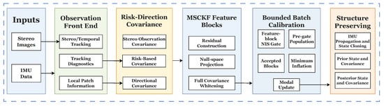
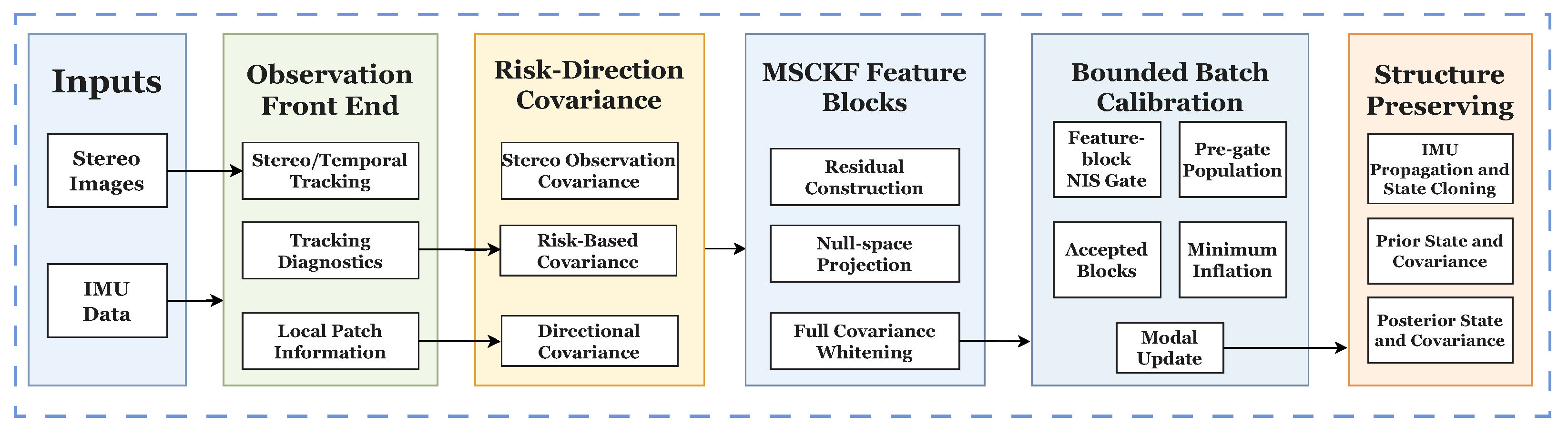
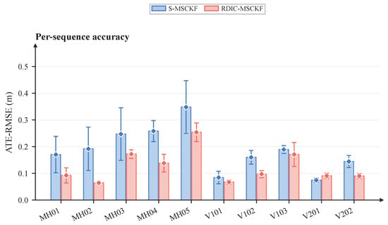
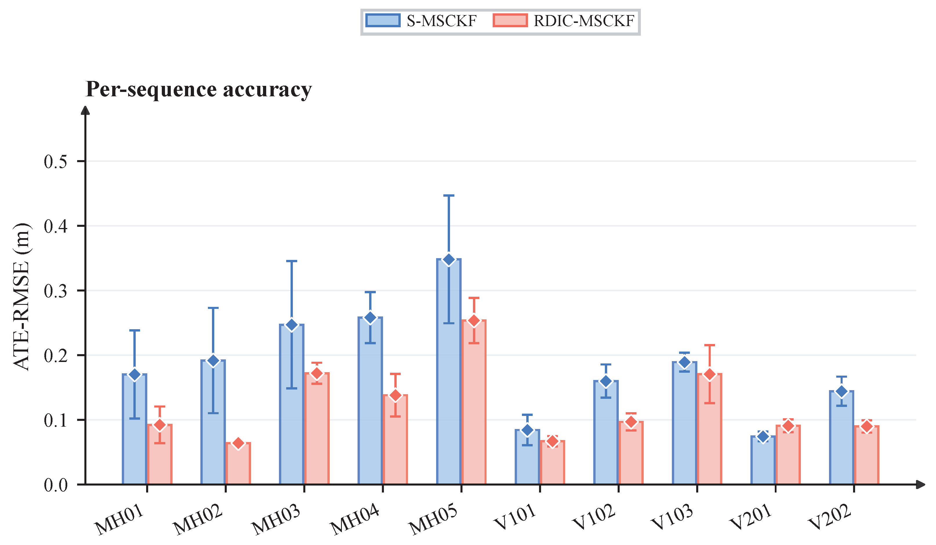
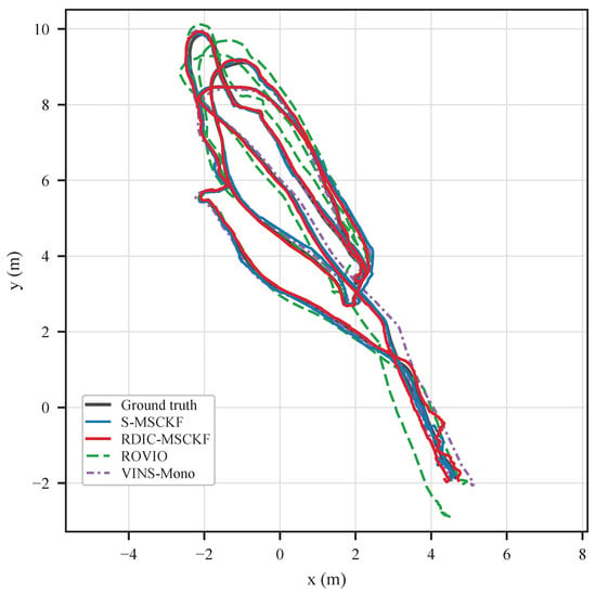
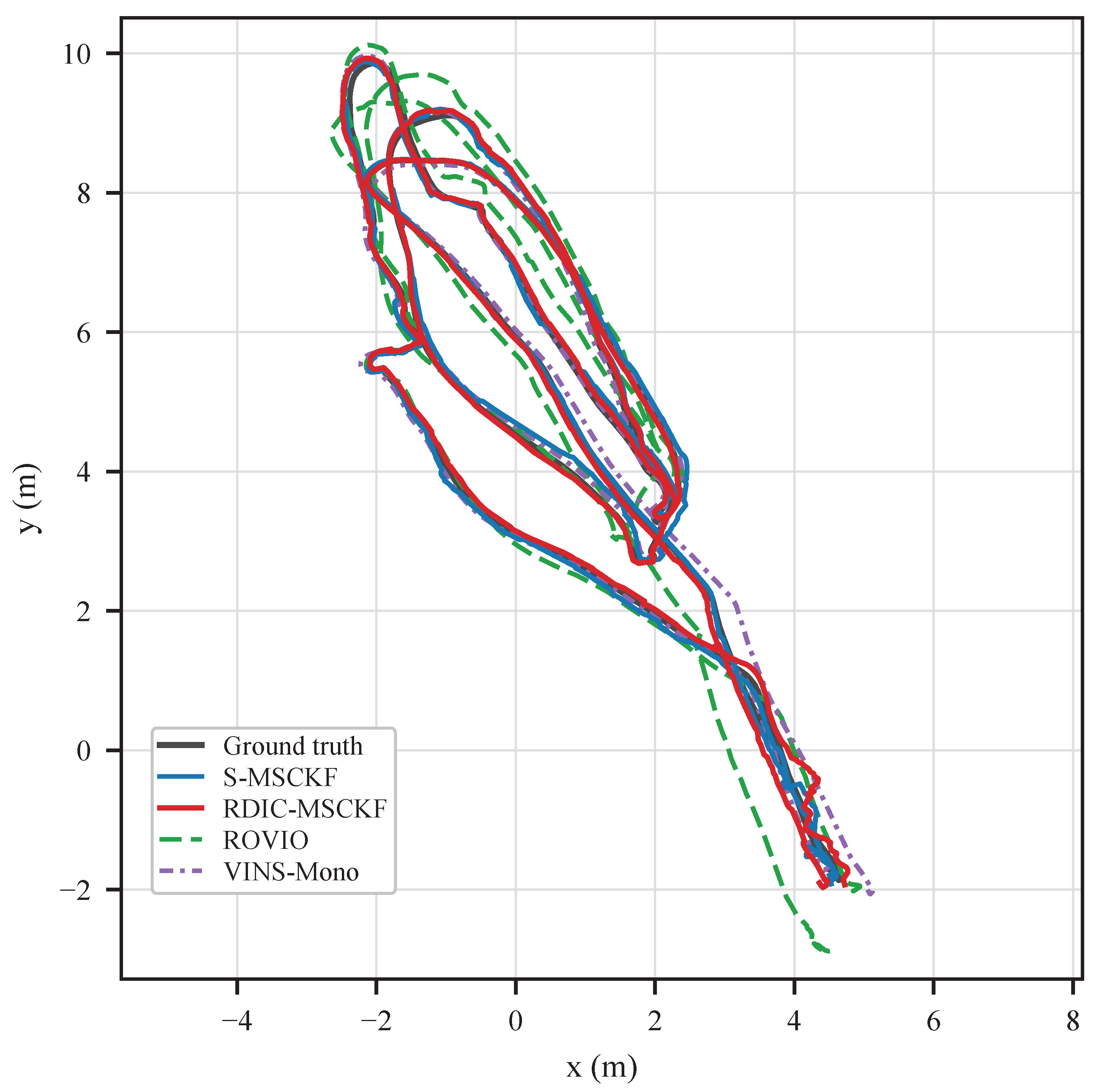
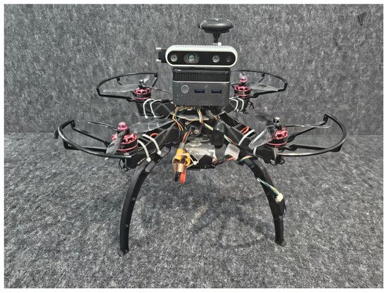
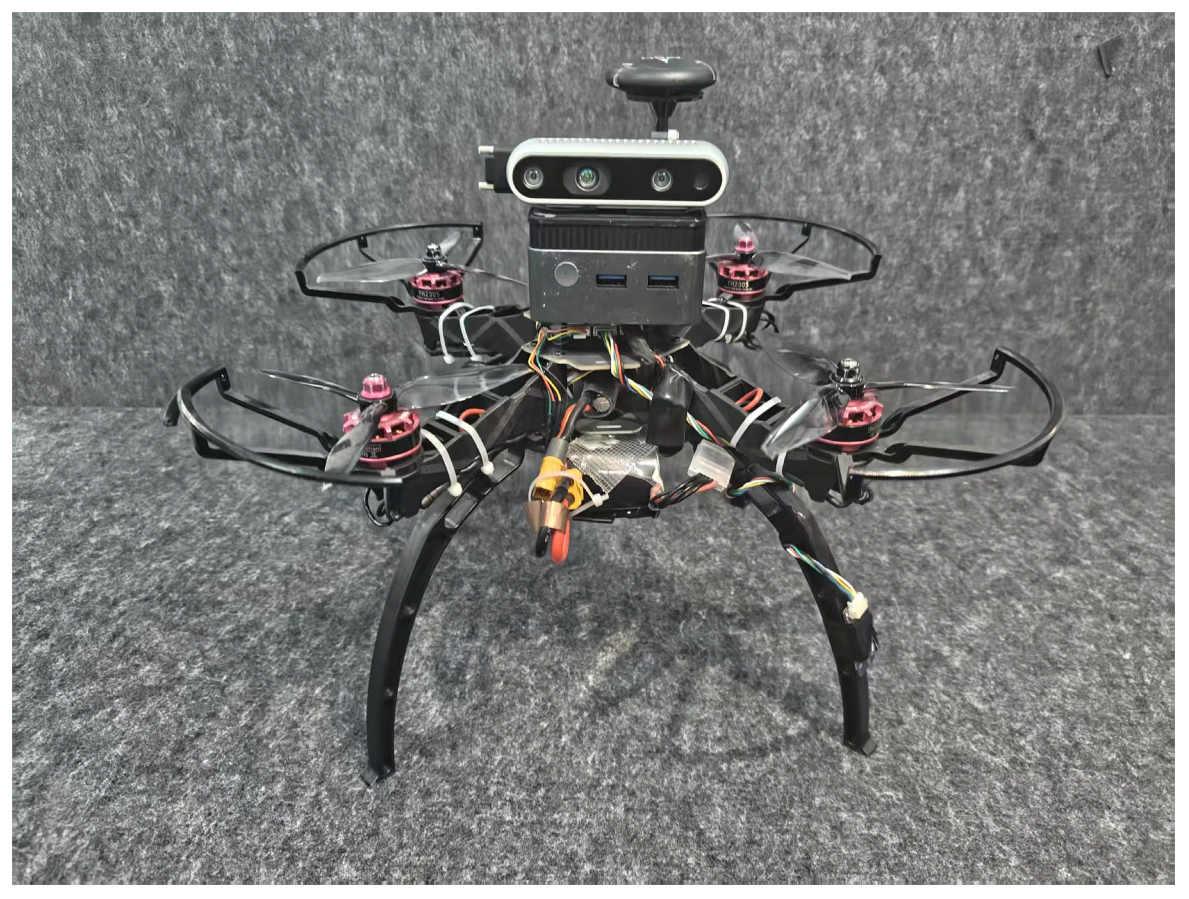
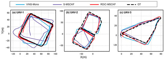
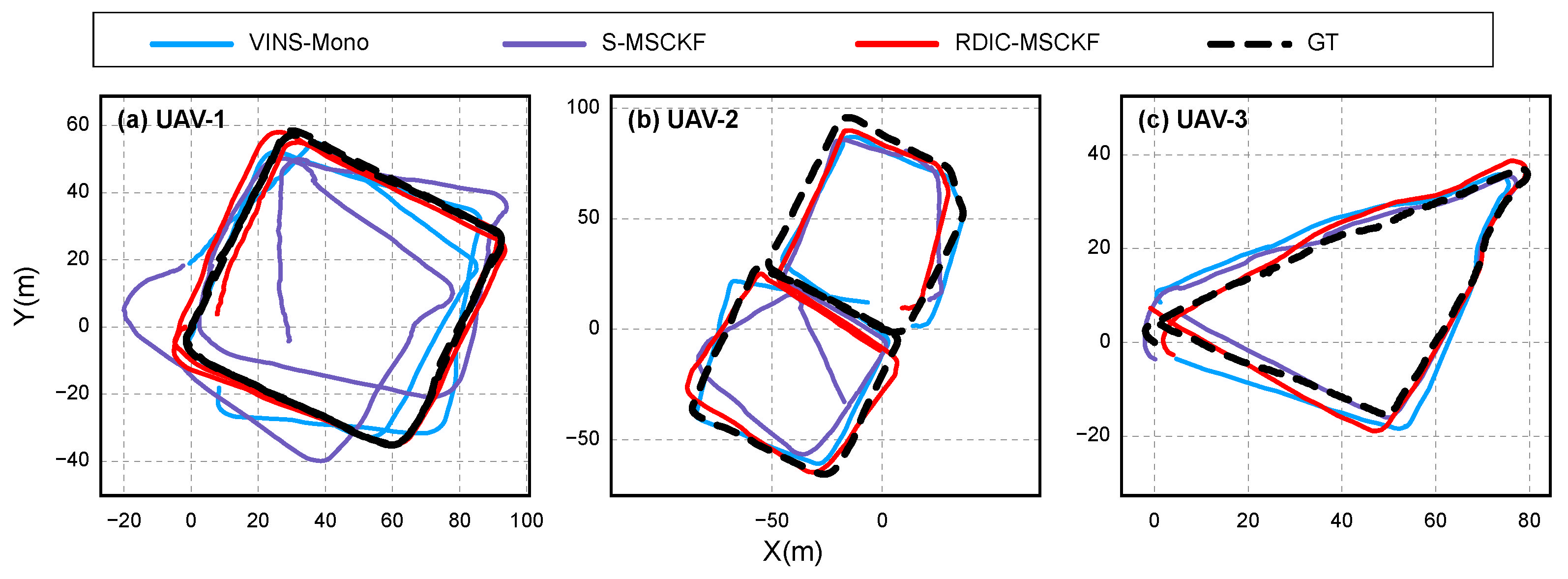
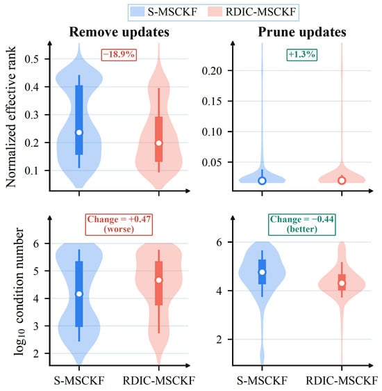
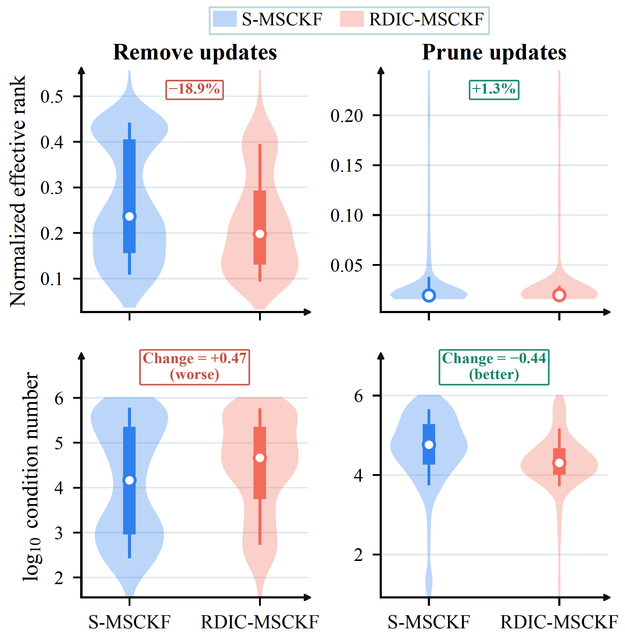
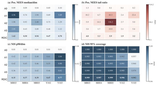
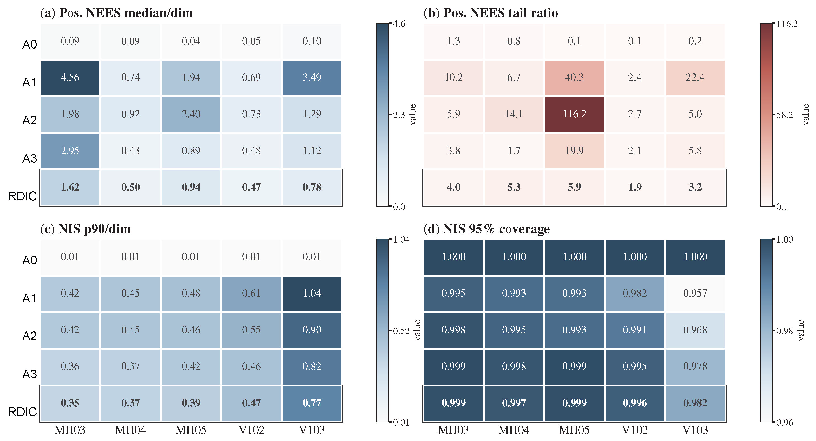
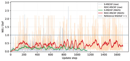
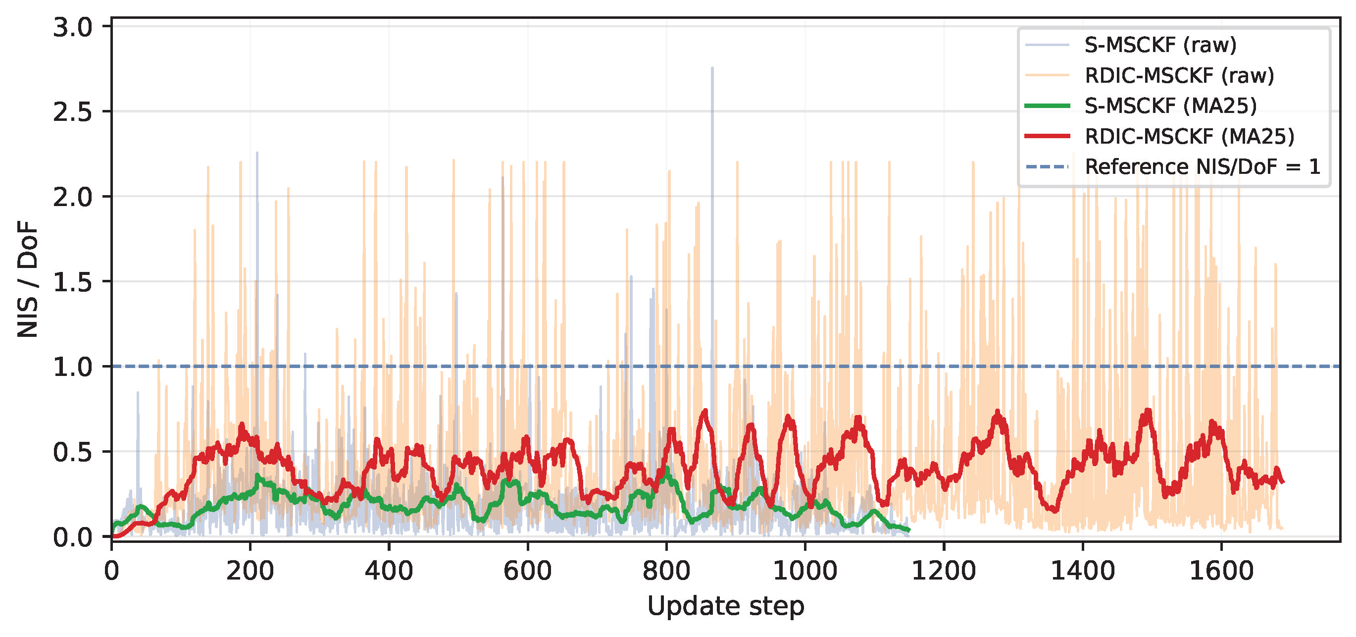
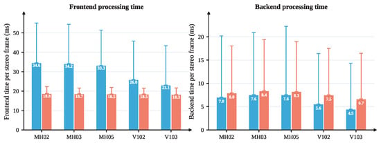
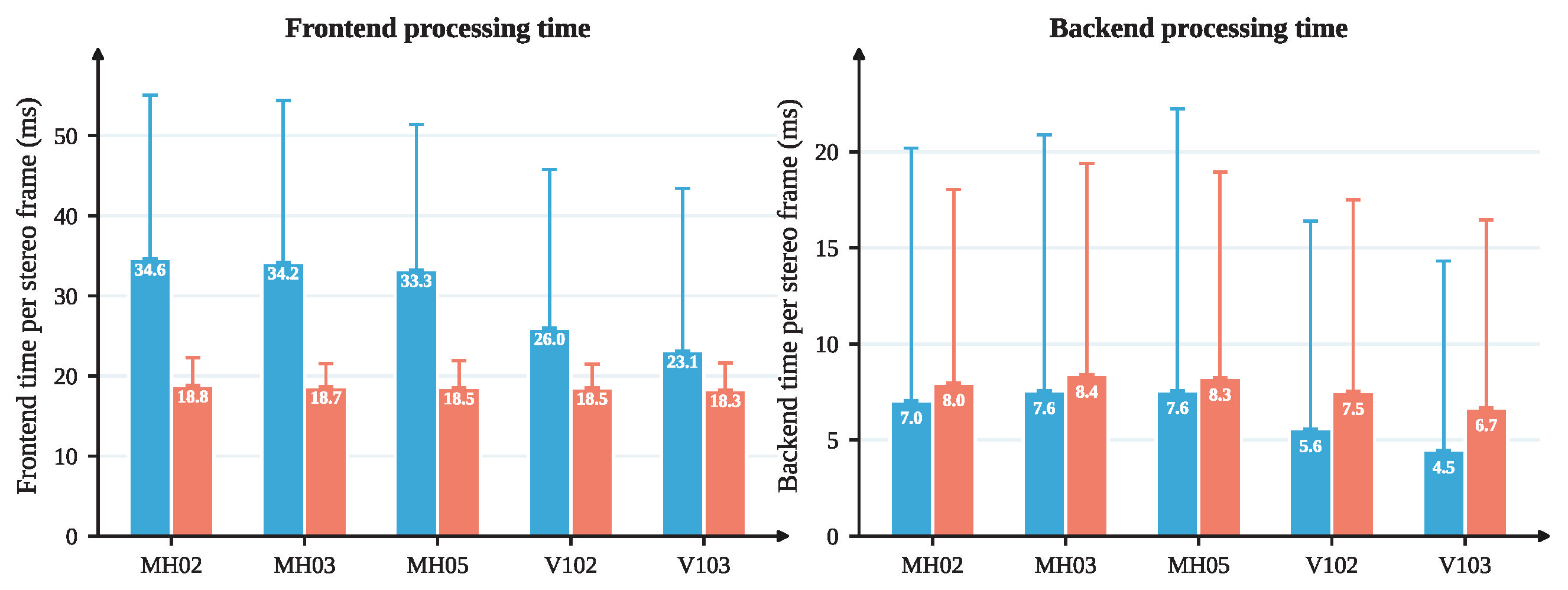
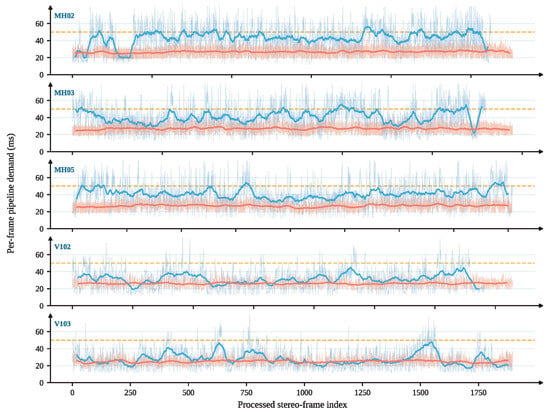
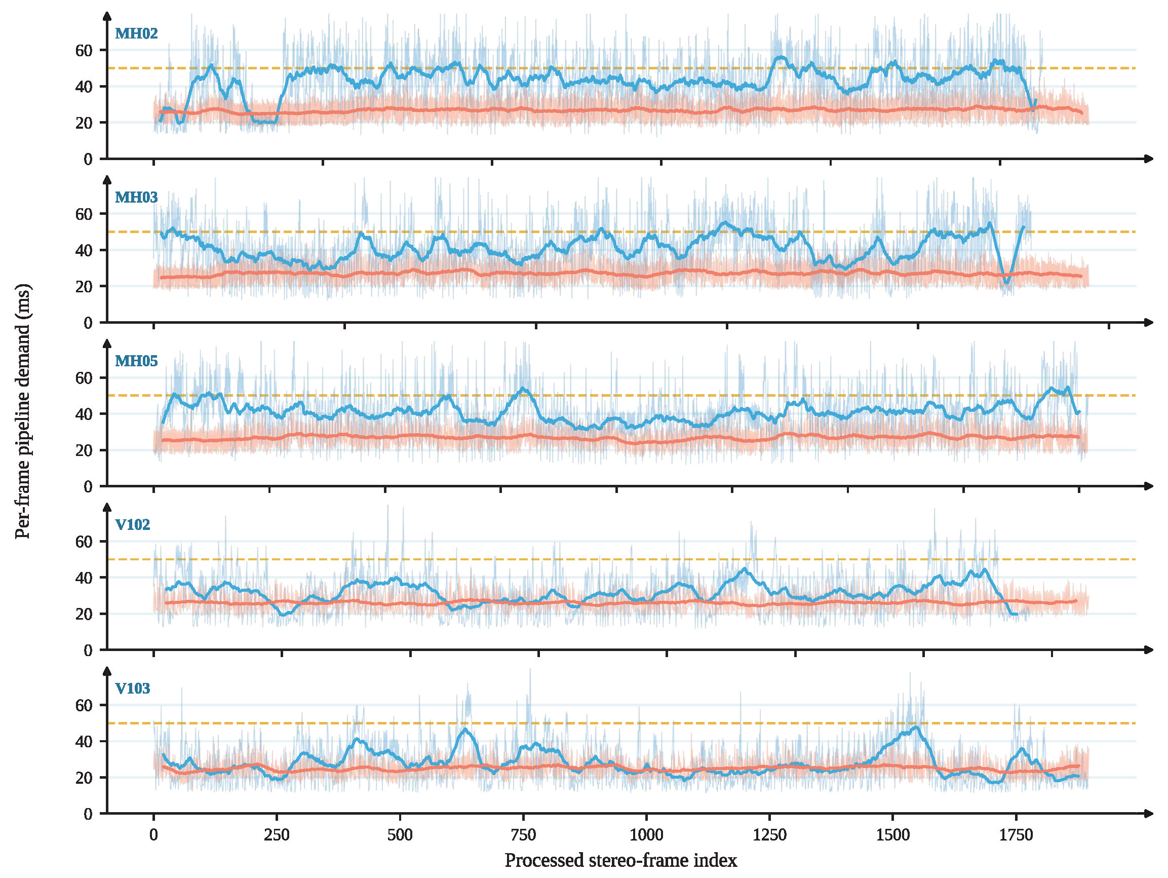

Disclaimer/Publisher’s Note: The statements, opinions and data contained in all publications are solely those of the individual author(s) and contributor(s) and not of MDPI and/or the editor(s). MDPI and/or the editor(s) disclaim responsibility for any injury to people or property resulting from any ideas, methods, instructions or products referred to in the content. |
© 2026 by the authors. Licensee MDPI, Basel, Switzerland. This article is an open access article distributed under the terms and conditions of the Creative Commons Attribution (CC BY) license.