Fuzzy Adaptive Impedance-Based Force and Position Compliance Control for Industrial Manipulators

Abstract

When a robot performs a grinding operation, the steady-state force/position tracking accuracy of its end-effector is critical to achieving high grinding quality. To solve this problem, a fuzzy adaptive impedance method is incorporated into the robot’s compliant control framework. Firstly, the robot dynamics model is established based on the Newton–Euler method. To describe the robot dynamics more comprehensively, a linear friction compensation model is also introduced. Secondly, a dynamic feedforward trajectory-tracking controller is proposed based on the dynamic model, and its stability is verified using a Lyapunov function. The impedance parameters are adjusted in real time according to the feedback contact force and its rate of change, thereby enabling dynamic equilibrium between the end contact force and end position. This allows the robot end-effector to exhibit compliance during external environmental interactions. Finally, a control platform of a force/position compliance controller was constructed, and two grinding conditions of plane and arc were designed to validate the effectiveness of force/position compliance control based on impedance control. Compared with the fixed impedance approach, the proposed method reduces overshoot by 11.6% (plane) and 12.45% (arc), improves surface roughness from Ra 0.042 μm to Ra 0.021 μm, and achieves faster force tracking with fewer oscillations.

1. Introduction

In recent years, intelligent and automated design in parts processing has become a key enabler of high quality, high efficiency, and low cost in the manufacturing industry [1,2,3]. Grinding is a part surface processing technology, and the main purpose is to obtain the specified surface roughness of the object. Traditional grinding work is usually done by workers with hand-held grinding tools, which leads to low efficiency and unstable grinding quality. In recent years, driven by the many advantages of industrial robots, research on robot automatic grinding has important application value and practical significance in the research of complex free-form surface grinding and polishing [4,5]. At present, the most widely used form is the robot force/position hybrid control and the force/position compliant control based on impedance control. To achieve high-precision control in unknown or varying environments, various intelligent algorithms have been incorporated, which can be broadly categorized into adaptive impedance control, neural network impedance control, fuzzy impedance control, and other methods [6].

The mechanism of robot position/force hybrid control is to realize position and force control, respectively, on two different orthogonal planes. The feedforward control is based on the dynamics model of the robot to compensate for the PID control, thereby improving the error convergence speed of the servo. Grotjahn and Heimann [7] analyzed and compared the two feedforward control models, designed the torque feedforward control algorithm including motor friction in each joint, and verified the effectiveness of the control method by taking the trajectory accuracy of industrial robots as the evaluation index. Asensio et al. [8] proposed a dynamic feedforward torque compensation algorithm based on the neural network prediction error model. By training the neural network with a set of trajectories, the torque required by any trajectory of the robot in the workspace can be calculated. The method is used to compensate the feedforward torque to the joint motor. The results show that the tracking accuracy of the end trajectory and the suppression of residual vibration are significantly improved. Zhang et al. [9] proposed a model-based feedforward control scheme to compensate for the joint friction caused by the friction generated by joint commutation in robot motion, and they tested the robot under static and dynamic conditions, which greatly improved the precision of joint inversion. Hamad and Karayiannidis [10] calculated the required torque value under the flexible joint and sent it as a feedforward quantity to the bottom of the servo driver to refresh the driver in real time. The flexible joint was controlled by superposition with the current output in the form of compensation.

Pfanne et al. [11] proposed a new object-level impedance control framework for torque-controlled robots to dexterously manipulate objects. By actively maintaining the required grasping force, it can adapt to the dynamic change in grasping force. Seraji and Howard [12] introduced an adaptive control algorithm into the traditional impedance control. For different environmental factors, the impedance coefficient is constantly adjusted to achieve a better coordination of the overall force and position. The experiment proves that the adaptive impedance control algorithm can overcome the interference of unknown environmental factors. Xu et al. [13] proposed an adaptive impedance control strategy that adjusts online according to external force feedback, and the contact force and target impedance control parameters of the robot interacting with the outside world can be adjusted in real time through fuzzy reasoning. Xing et al. [14] designed a new impedance control mode combined with an adaptive control scheme to solve the problem of unstable contact of the rotary valve. This control strategy can accurately track the axial position of the valve and improve the robustness of the whole system. Zahedi et al. [15] designed an adaptive impedance controller based on the feedback interaction force between the robot and the external environment, which can change the impedance control parameters according to the feedback interaction force. The impedance characteristics of the system are changed to realize a flexible characteristic when the robot has contact with the external environment. Gui et al. [16] proposed an adaptive method based on nonlinear model reference, which realized adaptive control by adjusting impedance parameters according to the error between the actual and the ideal end position. Zhang and Khamesee [17] used the adaptive control algorithm to obtain the reference motion trajectory online. The experimental results show that the control error of the reference motion trajectory could be within the allowable range, and the force tracking effect of the micro-instrument could be achieved. Zhang et al. [18] proposed a fuzzy neural network impedance control algorithm to adapt the impedance models with different stiffness characteristics of human body, which can improve the flexibility of the lower limb exoskeleton when interacting with the human body. Luo et al. [19] proposed a neural network architecture that could adjust the impedance controller according to external changes, which was a combination of reinforcement learning and operational space impedance controller. Yang et al. [20] proposed an adaptive impedance controller based on neural networks to compensate a series of uncertain disturbances in the system. The effectiveness of the control method is verified by Baxter robot experiments. Ren et al. [21] introduced an impedance model to improve the disturbance observer in order to improve the ability to adapt to the external environment. By observing the environment information and compensating the control system, the assembly task can be completed with less force error. Li et al. [22] proposed an end-to-end controller that deeply integrates image-based visual servoing (IBVS) with the Soft Actor-Critic (SAC) deep reinforcement learning algorithm. The network directly takes image features as input and outputs’joint torque or velocity commands, thereby bypassing the traditional 3D pose reconstruction stage. While these methods demonstrate improved adaptability over fixed-gain impedance, they suffer from two common drawbacks: (i) most of them simultaneously adjust multiple impedance parameters (inertia M, damping B, and stiffness K) based on heuristic rules or black-box learning, lacking a clear understanding of how each parameter individually affects the transient and steady-state response; (ii) the online tuning of M or K often introduces unwanted oscillations or steady-state force deviations, yet this critical trade-off has received little analytical attention in the existing comparative literature.

In recent years, fixed-time sliding mode control methods have attracted considerable attention for high-precision trajectory tracking of uncertain robotic systems. Hu et al. [23] proposed a robust adaptive fixed-time sliding mode control scheme for robotic systems with parameter uncertainties and input saturation, where an RBF neural network was employed to approximate the compound uncertainties, and nonsingular fast terminal sliding mode control was integrated to enhance robustness and convergence speed. Kang [24] developed an adaptive fixed-time sliding mode control framework for industrial manipulators, which effectively suppressed chattering through an adaptive reaching law and incorporated a third-order sliding mode observer for rapid estimation and compensation of uncertainties and disturbances; superior tracking accuracy and convergence performance were validated on a SAMSUNG FARA AT2 manipulator. Liu et al. [25] addressed fixed-time trajectory tracking for uncertain robotic systems by designing an adaptive RBF neural network to estimate model uncertainties and viscous friction, combined with a novel second-order fixed-time reaching law. The above studies mainly focus on trajectory tracking control, addressing robust tracking problems via fixed-time sliding mode and neural network approaches. However, in the context of force/position compliance control, how to further enhance the response speed and disturbance rejection capability of impedance control by leveraging the idea of fixed-time convergence remains an open issue. However, these methods treat the external environment as a pure disturbance and do not explicitly regulate contact forces, which is insufficient for grinding tasks where force quality directly determines surface integrity.

In this paper, a force/position compliant control method based on fuzzy self-adaptation is proposed. The impedance parameters were adjusted in real time according to the feedback contact force and its change rate, thereby achieving a dynamic balance between the end contact force and end position. Two grinding conditions of plane and arc surfaces were designed to verify the effectiveness of the proposed compliance control based on impedance control.

The rest of the paper is organized as follows. Section 2 presentsthe establishment of a dynamic feedforward trajectory tracking controller, covering both the robot dynamics model and the controller design. Section 3 describes the fuzzy adaptive impedance control method, including the construction of the fuzzy adaptive control system and an analysis of the influence of key parameters. Section 4 details the experimental verification of the force/position compliant control, where the method is validated on a robot grinding experimental platform. Section 5 summarizes the important conclusions of this study.

2. Establishment of Dynamic Feedforward Trajectory Tracking Controller

2.1. The Establishment of Robotic Dynamics Model

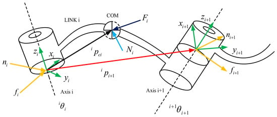
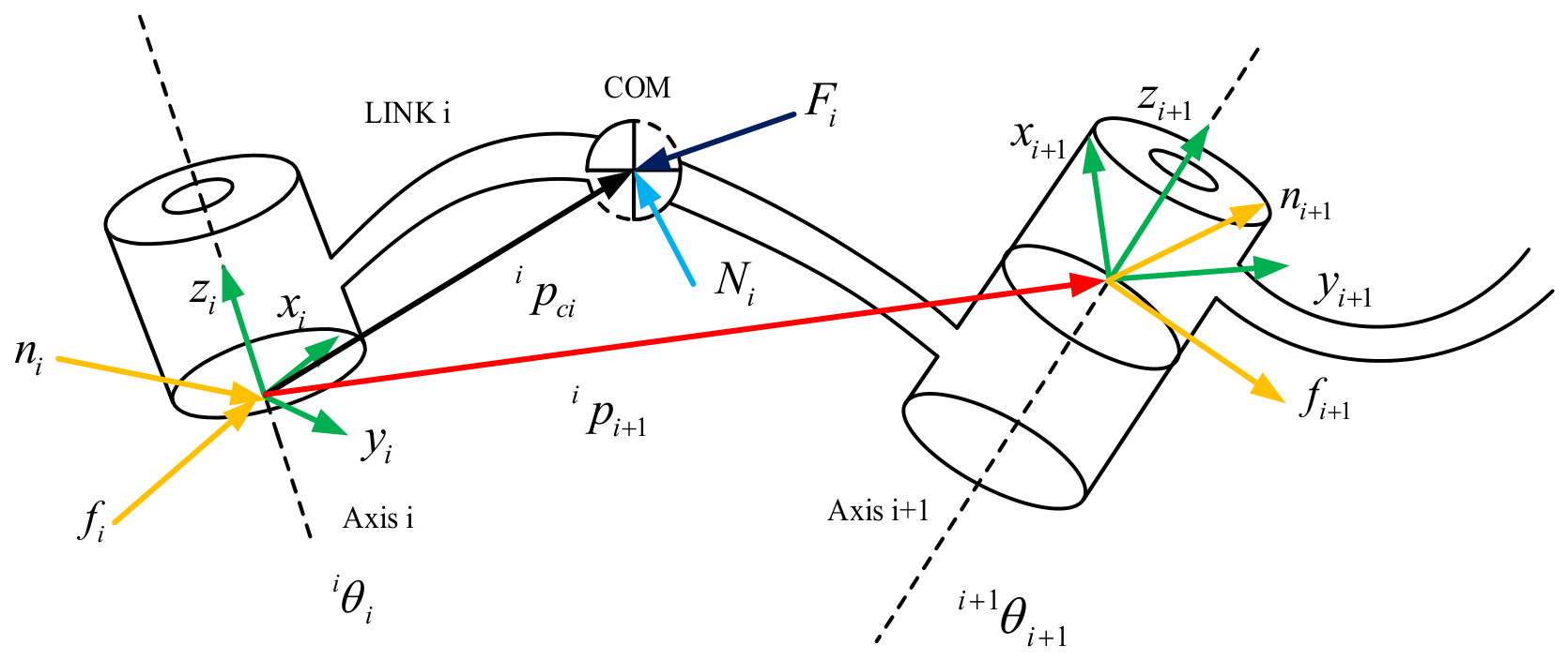
The dynamic model of the manipulator arm is established by Newton Euler method. The recursion diagram of force and moment between joints of robot as shown in Figure 1.

Figure 1. Recursive Newton-Euler force/moment propagation between adjacent links.

For a revolute joint, the recurrence equations for linearvelocity and angular velocity are as shown in Equations (1)–(4) [26]. ${\dot{\theta }}_{i+1}$ and ${\ddot{\theta }}_{i+1}$ are the angular velocity and angular acceleration of joint i + 1, ${}_i{}^{i+1}\mathit{R}$ is the transformation matrix from frame i to frame i + 1, ${}^{i+1}\mathit{P}_{\mathit{C}i+1}$ is the position of the i + 1 centroid coordinate system in the i + 1 rod coordinate system, and ${}^i\mathit{P}_{i+1}$ is the position of the i + 1 centroid coordinate system in the i rod coordinate system.

$${}^{i+1}\mathit{\omega }_{i+1}={}_i{}^{i+1}\mathit{R}^i{\mathit{\omega }}_i+{\dot{\theta }}_{i+1}{}^{i+1}Z_{i+1}$$

(1)

$${}^{i+1}\dot{\mathit{\omega }}_{i+1}{=}^{i+1}{\mathit{R}}^i{\dot{\mathit{\omega }}}_i{+}^{i+1}{\mathit{R}}^i{\mathit{\omega }}_i\times {\dot{\theta }}_{i+1}{}^{i+1}Z_{i+1}+{\ddot{\theta }}_{i+1}{}^{i+1}Z_{i+1}$$

(2)

$${}^{i+1}\dot{\mathit{v}}_{i+1}={}_i{}^{i+1}\mathit{R}\left({}^i\dot{\mathit{\omega }}_i{\times }^i{\mathit{P}}_{i+1}{+}^i{\mathit{\omega }}_i\times \left({}^i\dot{\mathit{\omega }}_i{\times }^i{\mathit{P}}_{i+1}\right){+}^i{\dot{\mathit{v}}}_i\right)$$

(3)

$${}^{i+1}\dot{\mathit{v}}_{\mathit{C}i+1}={\dot{\mathit{\omega }}}_{i+1}{\times }^{i+1}{\mathit{P}}_{\mathit{C}i+1}{+}^{i+1}{\mathit{\omega }}_{i+1}\times \left({}^{i+1}\mathit{\omega }_{i+1}{\times }^{i+1}{\mathit{P}}_{\mathit{C}i+1}\right){+}^{i+1}{\dot{\mathit{v}}}_{i+1}$$

(4)

The centroid moment of the connecting rod can be expressed as shown in Equation (5),

$${}^c\mathit{N}_i={}^c\mathit{I}_i{}^c\dot{\mathit{w}}_i+{}^c\mathit{w}_i\times ({}^c\mathit{I}_i{}^c\mathit{w}_i)$$

(5)

where c is the established centroid coordinate system of the rod. ${}^c\mathit{I}_i$ is the centroid inertia tensor of the rod.

The forces and moments are calculated as follows,

$${}^{i}f_i={}_{i+1}{}^i\mathit{R}{\cdot }^{i+1}{f}_{i+1}{+}^i{F}_i$$

(6)

$${}^{i}n_i{=}^i{\mathit{N}}_i{+}_{i+1}{}^i\mathit{R}{\cdot }^{i+1}{n}_{i+1}{+}^i{P}_{Ci}{\times }^i{F}_i{+}^i{P}_{i+1}\times {(}_{i+1}{}^i\mathit{R}^{i+1}\cdot f_{i+1})$$

(7)

In practice, joint friction is influenced by clearances among the robot joints, bearings, reducers, and other transmission components. The friction torque will affect the normal operation of the robot, causing end-effector vibration and unsatisfactory tracking accuracy. Therefore, it is necessary to establish an appropriate friction torque model and compensate for system deviation in real time according to the motor’s operating status. In this paper, a Coulomb-viscous friction model is used to characterize the joint friction torque and compensate for its influence on the overall dynamic model, as shown in Equation (8).

$${\tau }_f=f_c\cdot \mathrm{sgn}(\dot{q})+f_{\mathit{v}}\cdot \dot{q}$$

(8)

where $f_c$ is the Coulomb friction force, sgn(·) is the sign function, and $\dot{q}$ is the relative velocity of the component. $f_{\mathit{v}}$ is the coefficient of viscous friction, which is used to characterize the correlation between friction and lubrication.

By substituting Equation (8) into the Newton-Euler equation, the robot joint torque can be expressed as,

$${\tau }_i=\mathit{M}(q)\ddot{q}+\mathit{C}(q,\dot{q})+\mathit{G}(q)+{\tau }_f$$

(9)

According to the general dynamic expression, the joint torque ${\tau }_i$ of the robot is expressed as,

$${\tau }_i=\mathit{M}(q)\ddot{q}+\mathit{C}(q,\dot{q})+\mathit{G}(q)+f_c\cdot \mathrm{sgn}(\dot{q})+f_{\mathit{v}}\cdot \dot{q}$$

(10)

where, $\mathit{M}(q)$ is the inertia matrix of the robot, $\mathit{C}(q,\dot{q})$ is the Coriolis force and centrifugal force term, and $\mathit{G}(q)$ is the gravity term.

2.2. Design and Analysis of Dynamic Feedforward Trajectory Tracking Controller

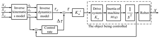
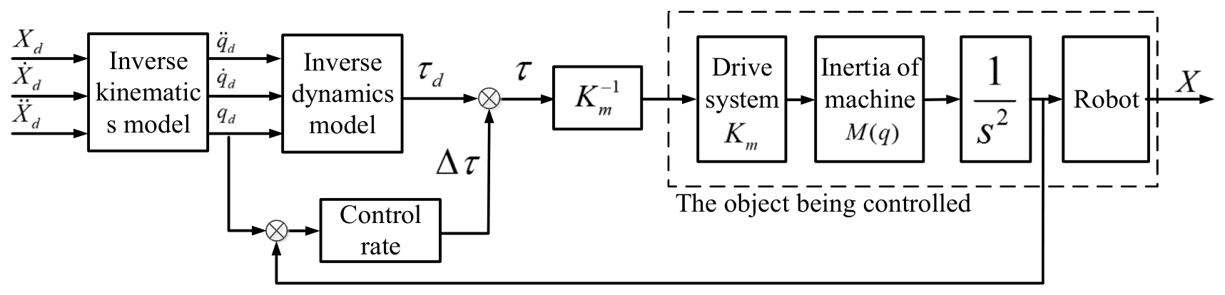
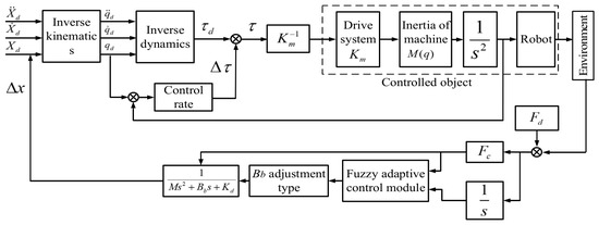
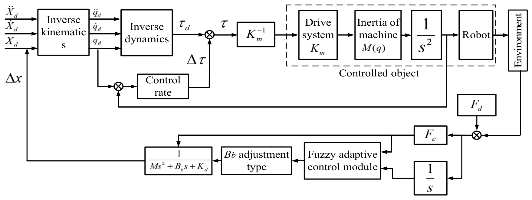
To improve the overall dynamic performance of the system without incurring significant computational overhead, a dynamic feedforward motion control structure is proposed. This scheme compensates for system dynamics and enhances trajectory tracking accuracy [27]. The control structure is shown in Figure 2.

Figure 2. Block diagram of the proposed dynamic feedforward control structure.

To demonstrate the trajectory tracking performance and dynamic response of the proposed dynamic feedforward control structure, its stability and robustness are verified using the Lyapunov method. To study the interaction between the robot end-effector and the environment, the joint-space dynamic equations are transformed into Cartesian space. Before proceeding with the stability proof, the following assumptions are made:

(i)

The robot dynamics are assumed to be known exactly for the feedforward part;

(ii)

The environment is modeled as a linear spring (F_e = k_e(x − x_e)) for the impedance analysis;

(iii)

The Jacobian matrix is assumed to be nonsingular within the workspace.

The dynamic relationship in Cartesian space is as follows,

$$F=\mathit{V}(q)\ddot{x}+\mathit{u}(q,\dot{q})+\mathit{p}(q)$$

(11)

where, $\mathit{V}(q)$ is the inertial matrix, $\mathit{u}(q,\dot{q})$ is the centrifugal force and Coriolis force vector, and $\mathit{p}(q)$ is the gravity vector in Cartesian space. $x$ is the end position vector, and F is the generalized operating force vector.

Based on the virtual work principle, the joint torque can be expressed as,

$$\mathit{\tau }={\mathit{J}}^{\mathit{T}}(q)\mathit{F}$$

(12)

The conversion relationship between velocity and acceleration in joint space and Cartesian space is shown as follows,

$$\dot{\mathit{x}}=\mathit{J}(q)\dot{q}$$

(13)

$$\ddot{\mathit{x}}=\mathit{J}(q)\ddot{q}+\dot{\mathit{J}}(q)\dot{q}$$

(14)

Multiply Equation (11) by ${\mathit{J}}^{\mathit{T}}(q)$ left, and substitute Equations (12)–(14) into Equation (11). It can be found that the dynamics equation in Cartesian space is related to the dynamics equation in joint space as follows,

$${\Lambda }_x=J^{-T}\left(q\right)\cdot M\left(q\right)\cdot J^{-1}\left(q\right)$$

(15)

$$u_x=J^{-T}\left(C\right(q,\dot{q}\left) - M\right(q\left)J^{-1}\dot{J}\right)J^{-1}$$

(16)

where ${\Lambda }_x$ is the inertia matrix in Cartesian space, $u_x$ is the centrifugal force and Coriolis force vector in Cartesian space, M(q) is the inertia matrix in joint space, C(q, $\dot{q}$) is the Coriolis and centrifugal matrix in joint space, J is the Jacobian matrix, and $\dot{J}$ is the derivative of the Jacobian matrix.

In actual working conditions, it is expected that the robot end effector can stably track the ideal position and complete a series of tasks. The control rate of the robot end F is determined by combining PD feedback control and dynamic feedforward control in the Descartes operating space, as shown in Equation (17).

$$F={\Lambda }_x(q){\ddot{x}}_d+{\mathit{u}}_x(q,\dot{q})\dot{\mathit{x}}+{\mathit{g}}_x(q)+{\tau }_{f,}{}_x(q,\dot{q})+{\Lambda }_x(q)(k_{\mathrm{p}}e+k_{\mathrm{d}}\dot{e})$$

(17)

where, $x_d$ is the ideal target position reached by the robot end at the current moment, ${\dot{x}}_d$ is the ideal target motion speed reached by the robot end at the current moment, $x$ is the actual motion position reached by the robot end at the current moment, $\dot{x}$ is the actual motion speed reached by the end of the robot at the current moment, and the parameters $k_{\mathrm{p}}$ and $k_{\mathrm{d}}$ are positive definite gain matrices. $k_{\mathrm{p}}$ represents the Proportional-action gain of the PD feedback term. $k_{\mathrm{d}}$ represents the derivative-action gain of the PD feedback term.

The control rate of the above formula can be expressed as,

$$F={\Lambda }_x(q){\ddot{x}}_d+u_x(q,\dot{q})\dot{x}+g_x(q)+{\tau }_{f,}{}_x(q,\dot{q})+{\Lambda }_x(q)k_{\mathrm{d}}({\dot{x}}_d-\dot{x})+{\Lambda }_x(q)k_{\mathrm{p}}(x_d-x)$$

(18)

The purpose of this control strategy is to return the position error and velocity error to 0. Here, the Lyapunov function is selected to analyze its stability, as shown in Equation (19).

$$\mathit{V}={\displaystyle \frac{1}{2}}{\dot{e}}^{\mathrm{T}}\dot{e}+{\displaystyle \frac{1}{2}}{e}^{\mathrm{T}}{K}_{p}e,e=x_d-x,\dot{e}={\dot{x}}_d-\dot{x}$$

(19)

where $\dot{\mathit{V}}(q)-2\mathit{u}(q,\dot{q})$ is a skew symmetric matrix and ${\dot{e}}^T\dot{\mathit{V}}(q)\dot{e}=2{\dot{e}}^T\mathit{u}(q,\dot{q})\dot{e}$.

$$\dot{\mathit{V}}=-{\dot{e}}^{\mathrm{T}}{K}_v\dot{e}\le 0,\ddot{e}+K_{\mathrm{d}}\dot{e}+K_{\mathrm{p}}e=0$$

(20)

According to $\dot{\mathit{V}}<0$ and ${\mathit{K}}_{\mathit{d}}>0$, when $\dot{\mathit{V}}=0$, the parameters $\dot{e},\ddot{e}$ are 0. In this case, $K_{\mathrm{p}}e$ is equal to 0. Since $K_{\mathrm{p}}$ has an inverse matrix, we know that $e$ is equal to 0. Regarding the condition when $\dot{\mathit{V}}=0$: From Equation (20), $\dot{\mathit{V}}=-{\dot{e}}^{\mathrm{T}}{K}_{\mathrm{d}}\dot{e}$ (since the skew-symmetric term cancels). Since $K_{\mathrm{d}}>0$, $\dot{\mathit{V}}=0$ if and only if $\dot{e}$ = 0. With $\dot{e}$ = 0, the closed-loop error dynamics (Equation (18)) further imply that $e$ must also be zero (because M_x is invertible). Thus $\dot{\mathit{V}}$ reaches zero only at the equilibrium point $\left[e^{\mathrm{T}},{\dot{e}}^{\mathrm{T}}\right]=\left[0,0\right]$. This proves asymptotic stability via LaSalle’s invariance principle.

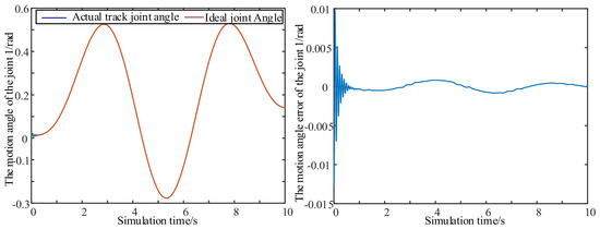
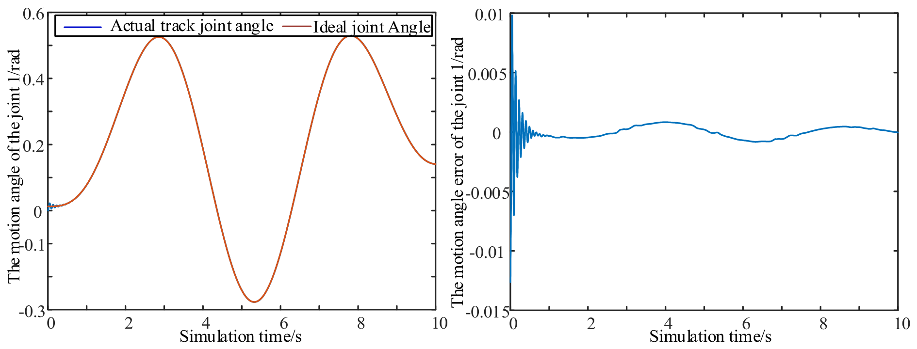
In Cartesian space, the dynamic feedforward control strategy combined with PD feedback achieves accurate tracking of both position and velocity. The stability of this control strategy is verified using the Lyapunov function. The tracking performance was evaluated under a given desired trajectory, and the results are shown in Figure 3, which shows the tracking performance of the dynamic feedforward trajectory together with the corresponding joint angle tracking errors. Initially, a slight transient oscillation is observed. As time progresses, the joint-angle tracking error stabilizes and gradually converges to zero. It can be seen that the dynamic feedforward trajectory tracking control based on the identified dynamic parameters exhibits satisfactory position and orientation tracking performance. This not only further proves the effectiveness of the identified dynamic parameters, but also confirms the feasibility of the dynamic feedforward trajectory tracking approach.

Figure 3. Tracking error of joint 1 angle between ideal and actual trajectories.

3. Analysis of Impedance Control Method Based on Fuzzy Adaptive

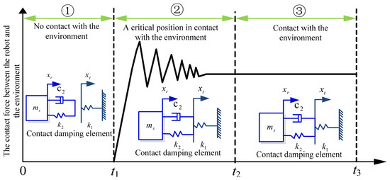
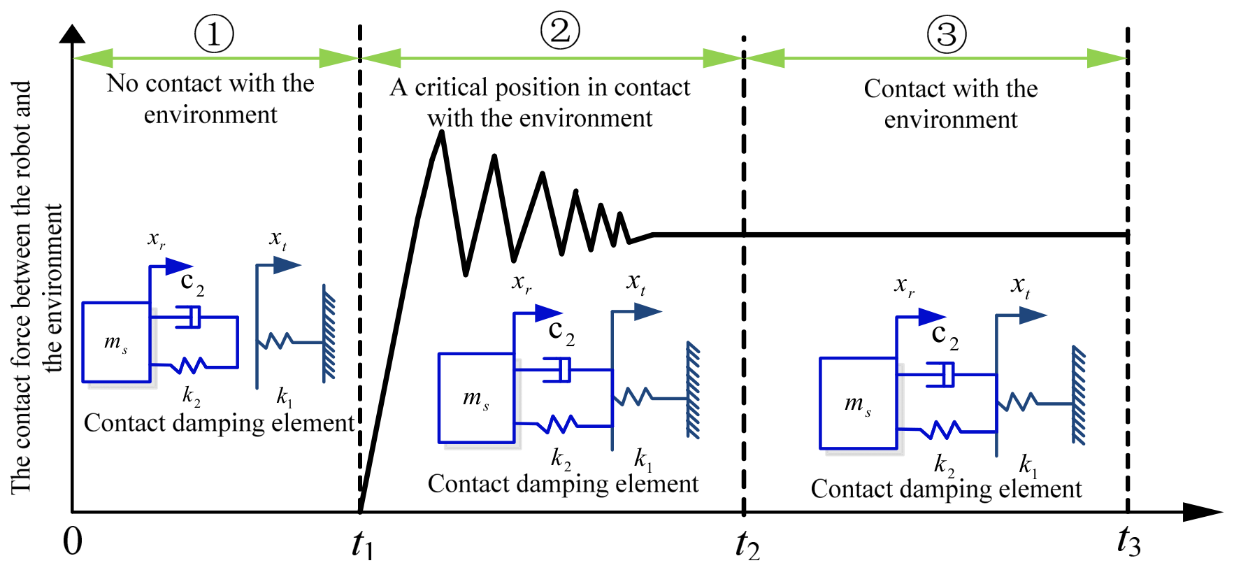
In impedance control, the interaction between the robot end-effector and the external environment is modeled as a second-order spring–mass–damper system. This control strategy coordinates the end-point force and position to achieve the desired position/force tracking performance. The environment is assumed to be rigid, and its mass, damping, and stiffness characteristics are denoted as M, B, and K respectively. The impedance regulating parameters are adjusted according to the real-time interaction behavior between the end-effector and the environment, thereby balancing the relationship between the end position and the contact force. A position increment is utilized to compensate the end position, ensuring the steady-state balance of the end contact force. Consequently, the end-effector exhibits admittance characteristics with respect to the environment, that is, the corresponding displacement output characteristics are generated under the action of external force input. The impedance principle and contact interaction force are depicted in Figure 4.

Figure 4. Relationship between robot end position and contact force.

In stage 1, there is no contact between the robot end-effector and the environment, and the contact force is zero. In stage 2, the end-effector initially interacts with the environment; at this moment, it collides with the environment and gradually stabilises. Notably, the very instant of contact triggers strong nonlinear collision transients, which the system must undergo before equilibrium can be reached. In stage 3, the contact force between the end-effector and the environment is generated and and tends towards a steady state, allowing the system to stably accomplish the desired contact task.In robot impedance control systems, feedback information such as end-effector position, velocity and interaction force with the environment is perceived. The interaction force is regulated indirectly through the second-order impedance characteristics. A commonly adopted ideal model for robot impedance control is,

$$\left\{\begin{array}{c}{M}_d({\ddot{X}}_d-{\ddot{X}}_r)+B_d({\dot{X}}_d-{\dot{X}}_r)+K_d(X_d-X_r)=\Delta F\\ \Delta F=F_d-F_e\end{array}\right.$$

(21)

If the external environment is an ideal spring, the impedance characteristic model of the robot is $F_e=K_e(X_d-X_e)$.

In general, the impedance model is chosen as a linear second-order system, characterized by the transfer function, $K(s)=1/(M{s}^2+Bs+K)$. The dynamic relationship between the force tracking error $\Delta F$ and the position disturbance E can be expressed as,

$$\begin{array}{l}{M}_d{\displaystyle \frac{d^{2}E(t)}{d{t}^2}}+B_d{\displaystyle \frac{dE(t)}{dt}}+K_{d}E(t)=\Delta F(t)\\ E=x_d-x_r\end{array}$$

(22)

In the impedance control framework, the position disturbance E is adopted to correct the reference position trajectory. The corrected reference trajectory is then given by $X_c=X_r+E=X_r+\Delta F\cdot K(s)$. When the robot end-effector tracks the corrected trajectory, the force tracking errors generated in all directions can be expressed as,

$$\Delta f=f_e-f_d=k_e(x_e-x_c)-f_d=k_e\times x_e-k_e(x_r+k(s)\times \Delta f)-f_d$$

(23)

Equation (24) is obtained by substituting $k(s)=1/(m{s}^2+bs+k)$ into the above equation,

$$\Delta f(m{s}^2+bs+k+k_e)=(m{s}^2+bs+k)[k_e(x_e-x_c)-f_d]$$

(24)

The steady-state force tracking error can be obtained from Equation (24) as follows,

$$\Delta f_{ss}={\displaystyle \frac{k}{k+k_e}}[k_e(x_e-x_c)-f_d]$$

(25)

For the steady-state force tracking error to be zero $\Delta f_{ss}=0$, the reference position must satisfy $x_c=x_e-f_d/k_e$. As shown in Equation (25), if the exact environment position and stiffness are known, the reference trajectory can be calculated from the above equation, thereby enabling accurate position tracking. However, the environmental position and stiffness are rarely known in advance. Consequently, the reference position cannot be precisely calculated to yield the ideal tracking force, and a finite force error inevitably remains. This results in a contact force that approaches the desired value asymptotically but never coincides with it.

The dynamic feedforward controller and the impedance controller are cascaded in our architecture. The impedance controller generates a position correction e (based on force error) to modify the desired trajectory, producing a corrected reference trajectory. The dynamic feedforward + PD controller then ensures that the robot end-effector accurately tracks this corrected trajectory with high bandwidth and small tracking errors. Therefore, the dynamic compensation error (due to model inaccuracies or friction) directly affects the actual position tracking error, which in turn influences the contact force because the force is determined by the deviation between the actual position and the environment. However, the fuzzy adaptive impedance loop is designed to be robust to moderate position errors by adjusting the damping parameter in real time, thus compensating for the residual tracking errors.

4. The Construction of Adaptive Control System

4.1. Construction of Fuzzy Adaptive Control System

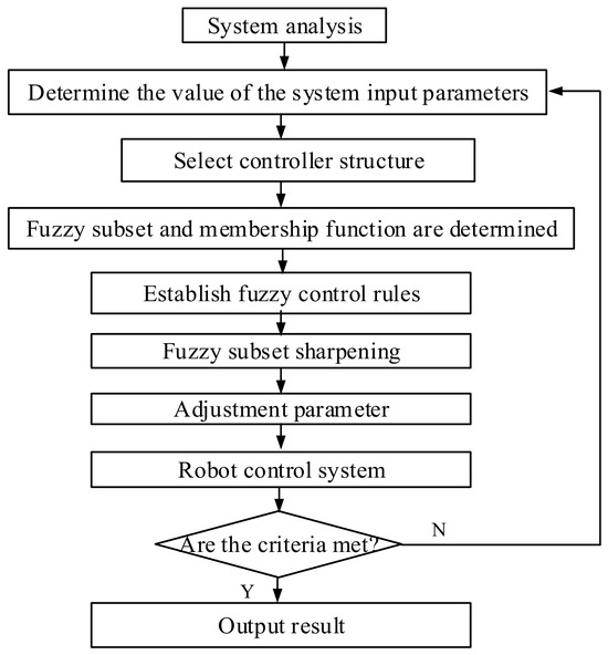
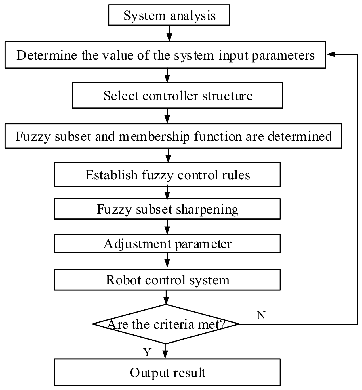
The logic block diagram of the fuzzy adaptive control scheme [28] is depicted in Figure 5. Firstly, the input variation rangeis normalized, a quantization series of the actual value is determined for the domain fuzzy variable, and the actual input value is transformed to the domain fuzzy variable in accordance with the normalized transformation logic. Secondly, based on the characteristics of the controlled system, an appropriate controller structure is selected, and both the fuzzy subset and the membership functions of the fuzzy variables are determined over the universe of discourse. The fuzzy control rules are derived from empirical knowledge. The fuzzy inputs are applied to these rules to compute the fuzzy outputs, which are subsequently defuzzified using the transformation logic to obtain the adjustment parameters.

Figure 5. Block diagram of fuzzy control system.

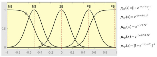
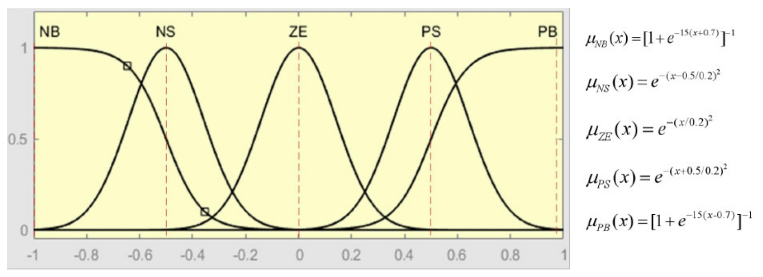
The fuzzy controller included input and output membership functions, a fuzzy control editor and a fuzzy control rule table. The fuzzy control editor selected domain, input variables and output variables, and five fuzzy subsets were established, as shown in Equation (26).

$$\left\{\begin{array}{c}{e}_f=[NB NS ZE PS PB]\\ {\dot{e}}_f=[NB NS ZE PS PB]\\ {\lambda }_b=[NB NS ZE PS PB]\end{array}\right.$$

(26)

By definition, a membership function is a subjectively defined function that is required to describe the continuity, stability, and gradual variation of fuzzy phenomena. The input and output membership function diagrams are shown in Figure 6.

Figure 6. The input and output membership function diagrams.

A two-input and single-output control rule was established, as shown in Table 1. To facilitate real-time adjustment, the fuzzy subsets mentioned above were further quantified and converted into fuzzy numbers. A fuzzy number provides an expression of fuzzy subset, which can convert NB, NS, ZE, PS, and PB into −2, −1, 0, 1, and 2, and the conversion results are shown in Table 2.

Table 1. The fuzzy rule table of two-input and single-output control.

${\mathit{e}}_{\mathit{f}}$	${\dot{\mathit{e}}}_{\mathit{f}}$
	NB	NS	ZE	PS	PB
NB	NB	NB	NS	NS	ZE
NS	NB	NS	NS	ZE	PS
ZE	NS	NS	ZE	PS	PS
PS	NS	ZE	PS	PS	PB
PB	ZE	PS	PS	PB	PB

Table 2. The formula type rule table of two-input and single-output control.

${\mathit{e}}_{\mathit{f}}$	${\dot{\mathit{e}}}_{\mathit{f}}$
	−2	−1	0	1	2
−2	−2	−2	−1	−1	0
−1	−2	−1	−1	0	1
0	−1	−1	0	1	1
1	−1	0	1	1	2
2	0	1	1	2	2

The fuzzy subsets above are converted to fuzzy numbers by Equation (27).

$${\lambda }_b=⟨(e_f+{\dot{e}}_f)/2⟩$$

(27)

where, ${\lambda }_b,e_f,{\dot{e}}_f$ are the representing fuzzy numbers for a certain link, and the symbol ⟨ ⟩ is the integration operator.

Fuzzy subsets −2, −1, 0, 1, and 2 are substituted into the transformation formula and can be written as,

$${\lambda }_b=⟨0.5\cdot e_f+(1-0.5)\cdot {\dot{e}}_f⟩$$

(28)

To achieve a wider range of adaptability, an adjustment factor $\alpha$ is introduced, which can be any value between 0 and 1, expressed as:

$${\lambda }_b=⟨\alpha \cdot e_f+(1-\alpha )\cdot {\dot{e}}_f⟩ , \alpha =0.5$$

(29)

The above control rules can be called "the F rule formula", and each adjustment factor corresponds to a control rule. This adjustment means that the influence weights of force deviation and force deviation change rate are different.

(1)

When $\alpha =0.5$, the force deviation and the force deviation change rate have the same weight on the output.

(2)

When $\alpha >0.5$, the weight of force deviation is greater than that of force deviation rate.

(3)

When $\alpha <0.5$, the weight of force deviation is smaller than that of force deviation rate.

The fuzzy rules are derived from expert knowledge and practical experience in force control: if the force error is large and increasing, the damping correction output is increased to quickly dampen the overshoot; if the error is small, the correction is reduced to avoid over-adjustment. The rule table (Table 1) follows the standard “if-then” format with five linguistic variables (NB, NS, ZE, PS, PB). Membership functions are chosen as triangular and trapezoidal functions, uniformly distributed over the normalized universe of discourse [−2, 2]. The conversion from fuzzy subsets to fuzzy numbers (Equation (27)) is based on the centroid method. For different tasks, the scaling factors (quantization and gain factors) may be adjusted to suit the force range and desired response speed, while the rule structure remains unchanged.

Based on real-time feedback, the characteristics of the controlled object and the control indexes are continuously modified, and the fuzzy control rules are adjusted accordingly. According to the distinct dynamic characteristics of the system, such as stability and response speed, appropriate fuzzy control rules are selected. When the force deviation is overly large, the system should promptly eliminate the influence resulting from the force deviation. By augmenting the regulating factor of the force deviation, the influence weight of the force deviation is increased, which enhances the system’s response speed while preserving stability. When the force deviation rate is excessively large, the system should rapidly reach the stability condition. In this case, the adjustment factor for the deviation rate is increased, and its weighting factor is raised, enabling the system to meet the stability requirement as soon as possible. Through the feedback of both the force deviation and the force deviation rate, the weighting factors of the adjustment parameters are changed in real time, so that any adverse impact of these two quantities on system stability is promptly eliminated.

4.2. The Robot End Force Tracking Based on Fuzzy Adaptive Control

When environmental stiffness and position are unknown, conventional impedance control with fixed parameters struggles to adapt to external variations, resulting in unsatisfactory force and position tracking. Moreover, abrupt changes in these environmental parameters render fixed impedance characteristics of the robot end-effector insufficient for maintaining stable interaction. To address this issue, a fuzzy adaptive control method is introduced, which adjusts the impedance control parameters online in response to real-time environmental changes, thereby enriching the system’s impedance behavior.

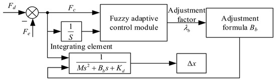
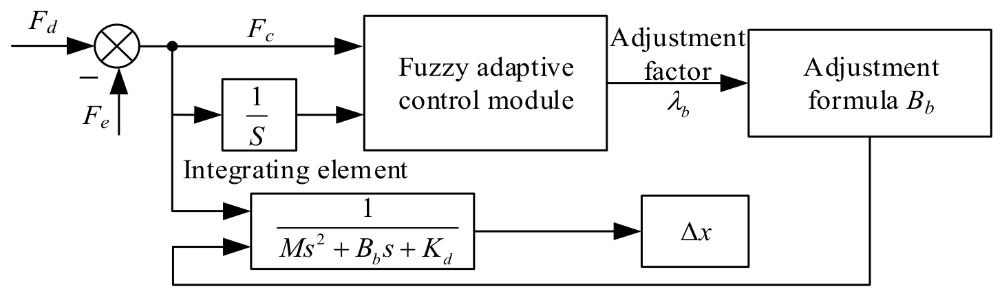
The double-input and single-output adjustment strategy was employed in this fuzzy adaptive control method. The inputs are the difference F_e between the ideal F_e and the actual tracking force F_d, and the rate of change of the tracking force error. Based on these input values, an adjustment factor for the impedance control parameter is generated, which is defuzzified to obtain the updated impedance control parameter. This updated parameter, in combination with the force error, is substituted into the impedance control law to derive the position correction. The contact force error and its rate of change work cooperatively to adjust the robot’s position command, thereby achieving a dynamic equilibrium between the contact force and position information. The control logic of fuzzy adaptive control for coordinating force and position adjustment is shown in Figure 7.

Figure 7. The block diagram of fuzzy adaptive control cooperative adjustment force and position information.

According to the above control strategy, the end-effector position can be continuously adjusted to achieve force tracking. Here, M, B, and K denote the desired inertia, damping, and stiffness matrices of the impedance model, respectively. Since force regulation is considered only along the contact direction, the corresponding scalar parameters are represented by m, b, and k. Similarly, uppercase symbols denote vector or matrix quantities, whereas lowercase symbols denote their scalar counterparts in the force-control direction. Therefore, F and f represent the force vector and scalar force, respectively, while E and e denote the position error vector and scalar position error, respectively.

For situations where the environmental stiffness is unknown or dynamically varying, defining the position tracking error as $e= x_e-x_r$ and the force tracking error as $\Delta f= f_e-f_d$, the impedance control model can be expressed as

$$\left\{\begin{array}{c}{F}_e-F_d=\mathit{M}({\ddot{x}}_e-{\ddot{x}}_r)+\mathit{B}({\dot{x}}_e-{\dot{x}}_r)+\mathit{K}(x_e-x_r)\\ \Delta f=f_e-f_d=m\ddot{e}+b\dot{e}+ke\end{array}\right.$$

(30)

When the interaction force is generated without contact with the environment, the expected contact force f_d = 0. When $\ddot{x}=0$ represents that the robot fits into the external environment, $\Delta f$ = 0 is obtained. This indicates that the robot end only finds the position of the contact environment without generating force/position information. At this time, any impedance parameter can meet the requirements of Equation (30).

When the robot end has an interaction force with the external environment, the expected contact force is not equal to 0. The expected contact force is the force/position information generated by driving the robot and the environment. At this time, there will be a certain collision and extrusion between the robot end and the environment, that is ${\ddot{x}}_e\ne 0$. As shown in Equation (31), the ideal steady-state condition $f_e=f_d$ can be satisfied if the stiffness coefficient of the impedance parameter k is set to 0. At this time, the error $\Delta f$ between the expected driving force and environmental contact force is 0.

$$\Delta f_{ss}={\displaystyle \frac{k}{k+k_e}}[k_e(x_e-x_c)-f_d]$$

(31)

Based on the above description, the impedance stiffness coefficient k can be set to zero to satisfy the steady-state tracking of the expected force and the contact force [28], and Equation (32) can be obtained.

$$\Delta f=f_e-f_d=m\ddot{e}+b\dot{e}$$

(32)

The contact force between the end of the robot and the environment can be replaced by $f_e=k_e(x_e-x_c)=-k_{e}e$, as shown in Equation (33).

$$-f_d=m\ddot{e}+b\dot{e}+k_{e}e$$

(33)

According to the above analysis, even if the end position and stiffness coefficient are unknown, the appropriate impedance parameters can be selected to achieve the effect of the expected force. Finally, the dynamic stability of the contact force can be achieved, that is $\Delta f=0$.

When the mutation in the position and stiffness coefficient of the external environment happens, $x_e$ is a time-varying variable. If ${\dot{x}}_e\ne 0$ and ${\ddot{x}}_e\ne 0$, the steady-state contact force error between the robot and the external environment $\Delta f$ is not equal to 0. In order to achieve the steady-state contact force between the robot and the external environment, it is necessary to reflect the changes in the impedance parameters synchronously according to the changes in the external environment.

A fuzzy adaptive control algorithm was introduced to compensate for the effects of errors caused by changes in time and environment. Considering the stability of the control system, it was not recommended to modify the quality coefficient in real time. The adjustment of the mass coefficient will shock the whole system, which is not conducive to the stability of force tracking. According to the force error and force error rate of external feedback, the adjustment factor of damping coefficient ${\lambda }_b$ can be obtained by substituting it into the fuzzy adaptive control algorithm. The adaptive control rate of the whole system can be expressed as,

$$\Delta f=f_e-f_d=m\ddot{e}+(b+\Delta b(t))\dot{e}$$

(34)

$$\Delta b(t)=\left\{\begin{array}{l}{\lambda }_b{b}_{\max }, {\lambda }_b\ge 0\\ {\lambda }_b(b(t-1)-b_{\min }), {\lambda }_b\le 0\end{array}\right.$$

(35)

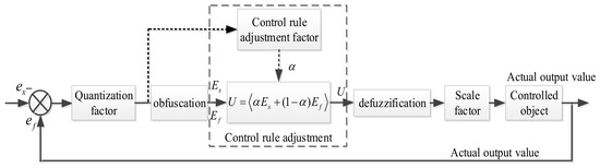
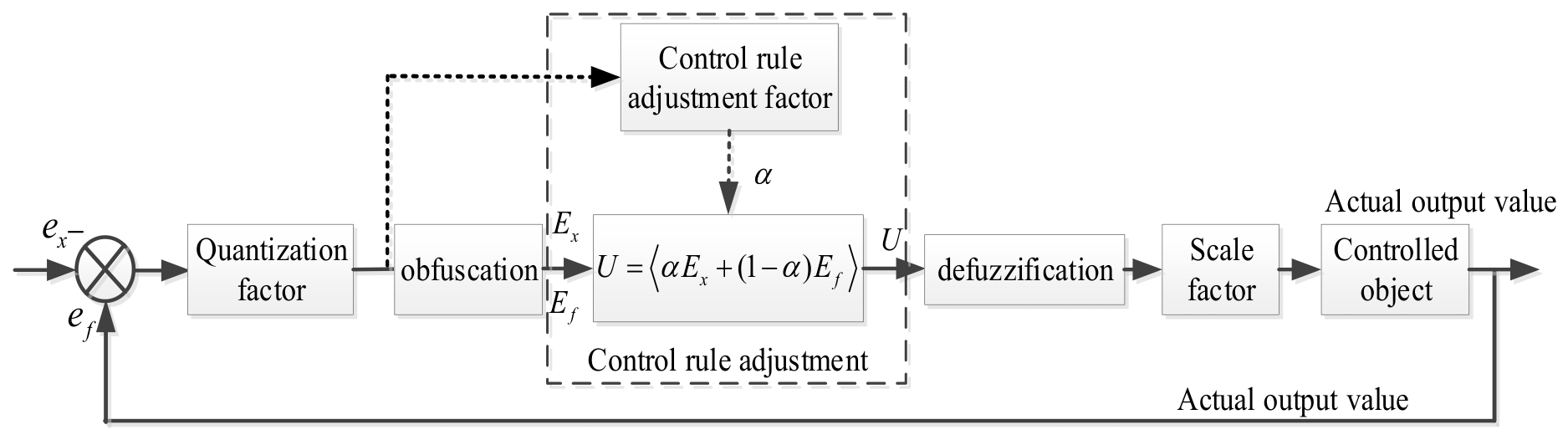
For the adjustment mechanism of the parameter ${\lambda }_b$, the corresponding fuzzy control rule self-adjustment analytic expression and logic block diagram are shown in Figure 8.

$$\left\{\begin{array}{l}U=\alpha E_f+(1-\alpha ){\dot{E}}_f\\ \alpha (t+1)=\alpha (t)-\gamma \cdot \mathrm{Sgn}(E_f-{\dot{E}}_f)\end{array}\right.$$

(36)

where U denotes the fuzzy adaptive input, $\alpha$ is the weighting factor, and $\gamma$ is the adaptive learning rate. To be better applied to the robot control system, the above formula can be converted into discrete format.

$$\left\{\begin{array}{c}\ddot{X}(t)={\displaystyle \frac{1}{M_d}}(\Delta F(t)-B_d{\dot{X}}_c(t)-K_d{X}_c(t))\\ {\dot{X}}_c(t)={\dot{X}}_c(t-1)+{\ddot{X}}_c(t)\cdot T\\ X_c(t)=X_c(t-1)+{\dot{X}}_c(t)\cdot T\end{array}\right.$$

(37)

where X_c denotes the displacement compensation generated by the impedance controller, and M_d, B_d, and K_d are the desired impedance parameters.

Figure 8. The block diagram of fuzzy control rules in the self-adjusting method.

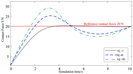
To sum up, the impedance control logic block diagram with fuzzy adaptive control is shown in Figure 9.

Figure 9. Impedance control logic block diagram with fuzzy adaptive control.

4.3. Characteristic Analysis of Fuzzy Adaptive Impedance Control Parameters

In an adaptive impedance control system, the impedance parameters serve as adjustment factors that are continuously updated based on external feedback. By selecting appropriate impedance parameters for different applications, effective force/position compliant tracking can be achieved. The desired inertia, damping, and stiffness parameters each exert distinct influences on system stability and also determine the compliance of the robot end-effector with the external environment. To investigate the effect of each impedance parameter on system stability, a robot impedance/admittance control system was built using Simulink in Matlab R2020b software, and simulation experiments were conducted by varying one parameter at a time while keeping the other two constant, following the control-variable method.

(1)

Analysis of influence of quality parameters $M_d$ on stability of control system

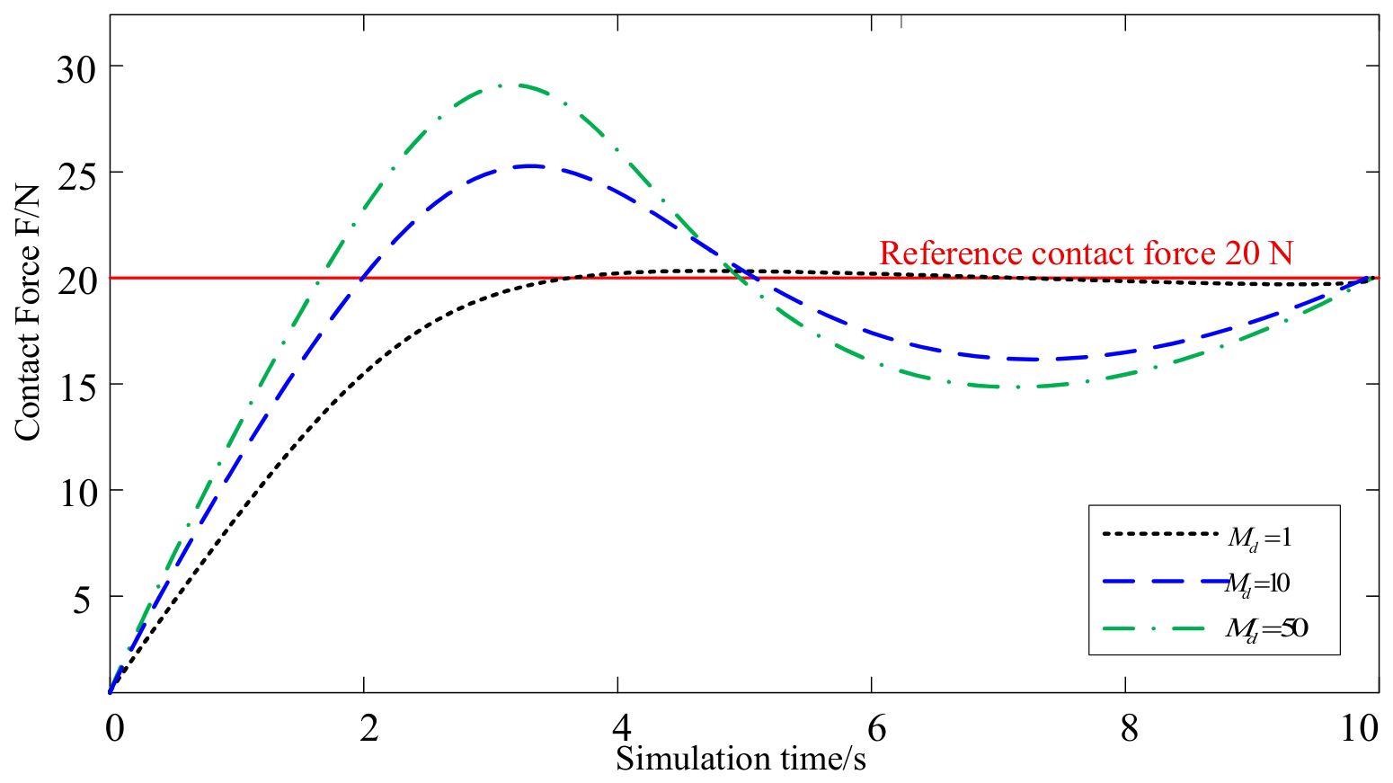
The impedance control parameters $B_d=100$ and $K_d=1$ are fixed, and the inertia parameter $M_d$ is changed to 1, 10, 50, respectively. The simulation results are shown in Figure 10.

Figure 10. Influence of inertial parameters $M_d$ on system stability.

The simulation results indicate that as the desired inertia parameters increase, the interaction force between the robot and the environment begins to oscillate with progressively growing amplitude. Although the system maintains stable force tracking for an extended period, the overall stability of the control system tends to decline. On the basis of these observations, the desired inertia parameters should be kept within a relatively small range to ensure rapid and stable force tracking. Moreover, improved force/position compliance can be achieved by appropriately combining the desired damping and stiffness parameters with the inertia parameters.

(2)

Analysis of the influence of the damping parameter $B_d$ on the stability of the control system

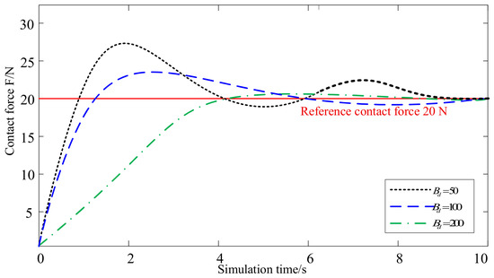
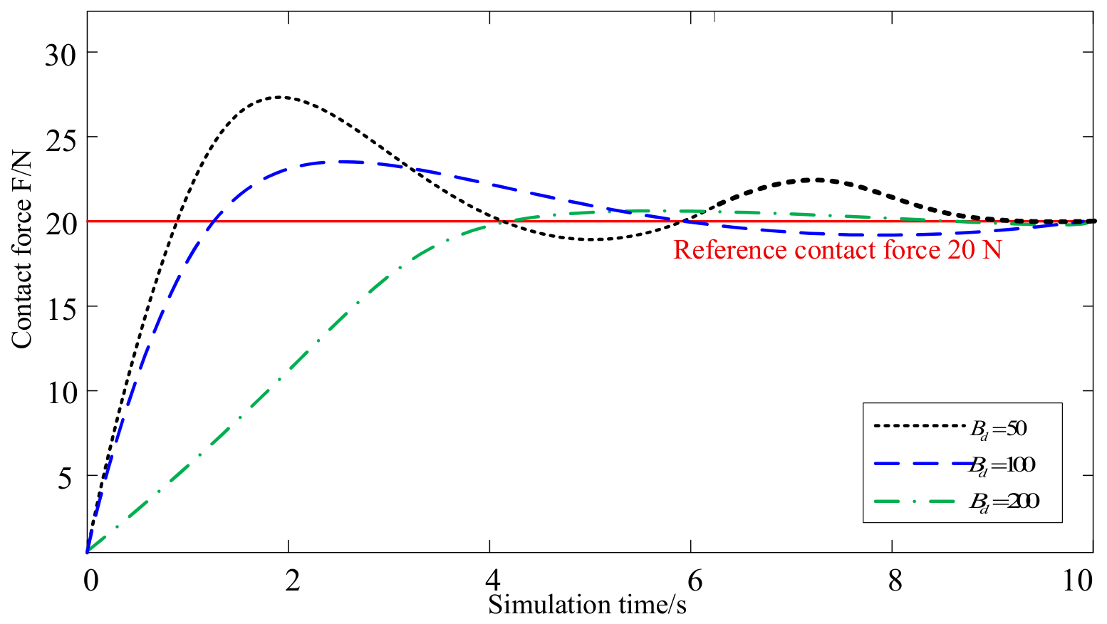
The impedance control parameters $M_d=1$ and $K_d=1$ are fixed, and the damping parameter $B_d$ is changed to 50, 100, and 200, respectively. The simulation results are shown in Figure 11.

Figure 11. Influence of damping parameters $B_d$ on system stability.

The results show that as the damping parameter gradually increases, the overshoot of the interaction force between the robot and the external environment decreases progressively. However, the damping parameter has little effect on the steady-state contact force at the end-effector. Increasing the damping parameter can smooth the contact force of the end force, and increasing the damping parameter will increase the tracking time of the system. This indicates that the damping parameters will affect system stability to a certain extent. Therefore, when designing an impedance control system, it is necessary to select appropriate impedance parameters, and achieve force/position compliance tracking control with suitable desired inertia and stiffness parameters.

(3)

Analysis of the influence of the stiffness parameter $K_d$ on the stability of the control system

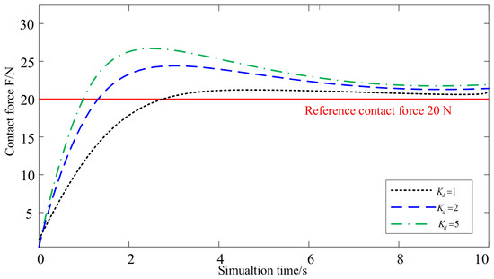
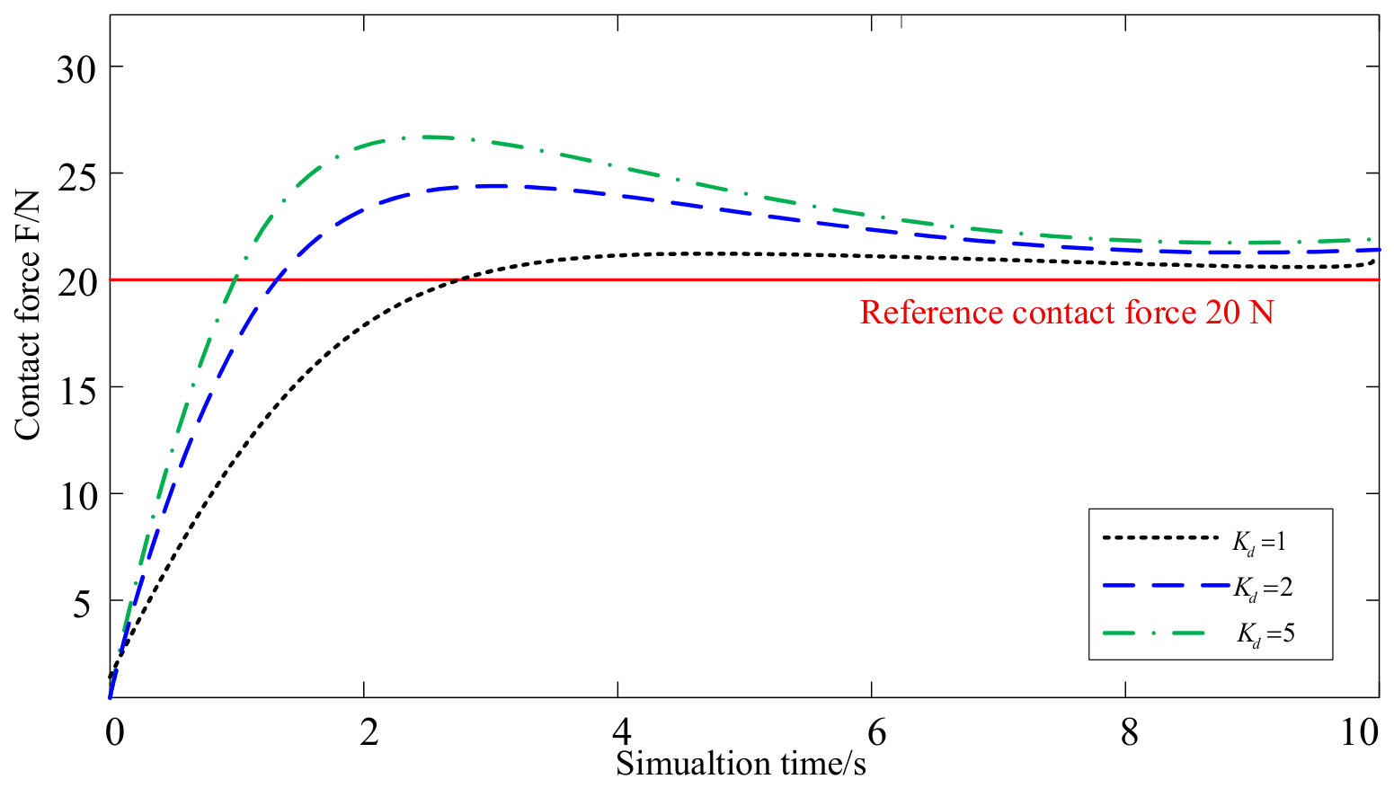
The impedance control parameters $M_d=1$ and $B_d=100$ are fixed, and the stiffness parameter $K_d$ is changed to 1, 2, and 5, respectively. The simulation results are shown in Figure 12.

Figure 12. Influence of stiffness parameters $K_d$ on system stability.

The results show that as the stiffness parameter increases, the force tracking speed improves accordingly. However, the steady-state error of the contact force also increases, and a larger stiffness coefficient leads to faster convergence to the desired contact force, which may cause overshoot in the force tracking effect. Conversely, reducing the stiffness coefficient decreases the force tracking error but prolongs the settling time. Therefore, the stiffness parameter should be selected based on the specific interaction between the control system and the external environment. When the stiffness parameters are adjusted, it is essential to ensure that the system remains in a critically damped or overdamped state to maintain stability.

Based on these results, inertia adjustment (M) tends to induce oscillations and prolong settling time, making the system prone to instability. Stiffness adjustment (K) reduces rise time but increases steady-state force error and may cause overshoot, as shown in Figure 11. Damping adjustment (B), on the other hand, effectively smooths the force response and reduces overshoot without introducing steady-state error, and it has a milder impact on stability. Thus, while online stiffness adjustment is possible, it would risk force overshoot and larger steady-state deviationsboth undesirable for grinding quality. We therefore opted for damping adaptation as a safer and more effective strategy.

5. Experimental Verificationof Force/Position Compliance Control

5.1. The Construction of the Experimental Platform

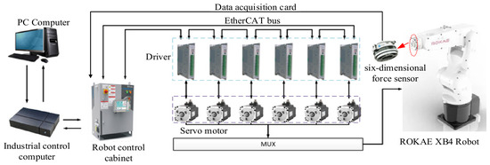
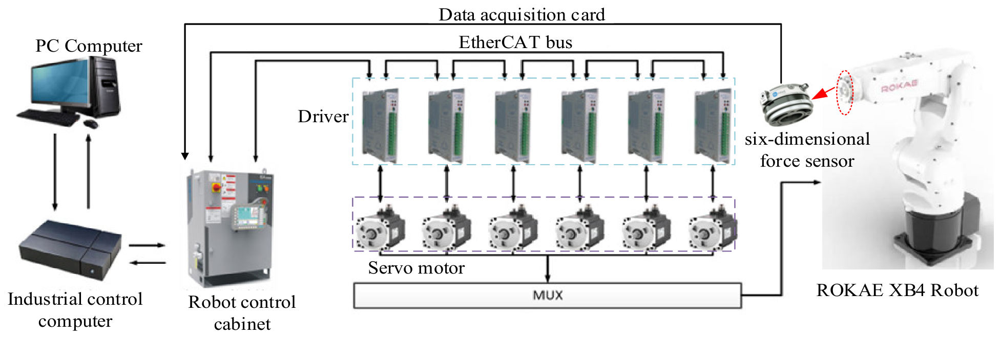
Based on the distributed architecture of EtherCAT real-time industrial bus protocol, the robot control system features modularity, real-time performance, and support for secondary development. The system mainly comprises a ROKAE XB4 six-axis industrial robot (ROKAE, Jining, China), a PC, an industrial computer, and a robot control cabinet that houses both the drivers and the controller. The robot controller is built based on the industrial control computer, which integrates and encapsulates the robot control and motion control modules. To enable EtherCAT communication, this industrial computer is equipped with the EtherCAT master protocol stack developed by Acontis (Weingarten, Germany). The protocol stack adopts a modular structure, and provides astandard interface between the software modules and the functional modules, allowing different application requirements to be met through module replacement. It is integrated into the S20-HJC1 industrial computer (Wenxin, Suzhou, China) to serve as the communication master station. The specific implementation of the experimental platform is shown in Figure 13.

Figure 13. The framework of the control system of the experimental platform.

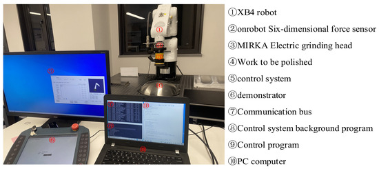
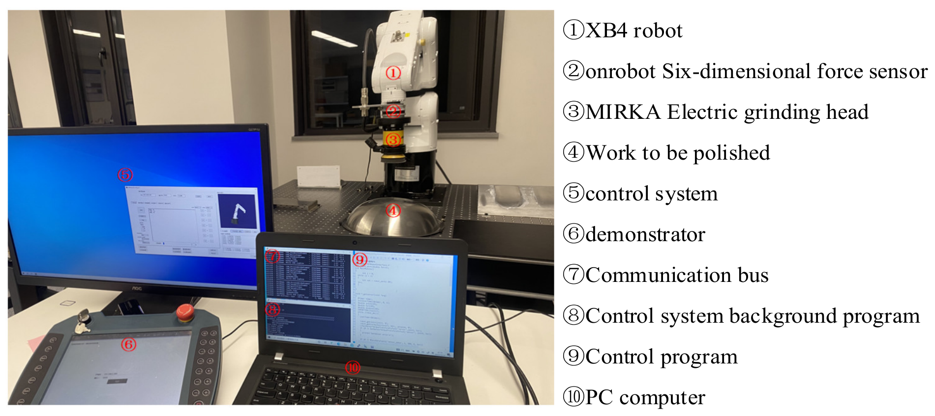
In order to verify the effectiveness of the control algorithm for steady-state tracking of end contact force, an Onrobot six-dimensional force sensor (Onrobot, Odense, Denmark), (technical parameters are shown in the Table 3) and an electric grinding (Mirka AIROS 350 NV, Jeppo, Finland) were installed at the end of the XB4 robot. The grinding experiments in various environments can be realized based on the experimental platform, as shown in Figure 14.

Table 3. The technical parameters of six-axis torque sensor.

Conventional Characteristic	Six-Axis Torque Sensor				Unit
	${\mathit{F}}_{\mathit{x}\mathit{y}}$	${\mathit{F}}_{\mathit{z}}$	${\mathit{T}}_{\mathit{x}\mathit{y}}$	${\mathit{T}}_{\mathit{z}}$
range	200	200	10	5.5	[N] [N.m]
Resolution	0.2	0.8	0.01	2 × 10−3	[N] [N.m]
IP level	67
dimension	50 × 71 × 93 mm

Figure 14. Grinding experimental platform prototype.

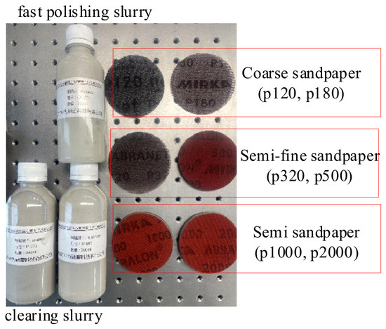
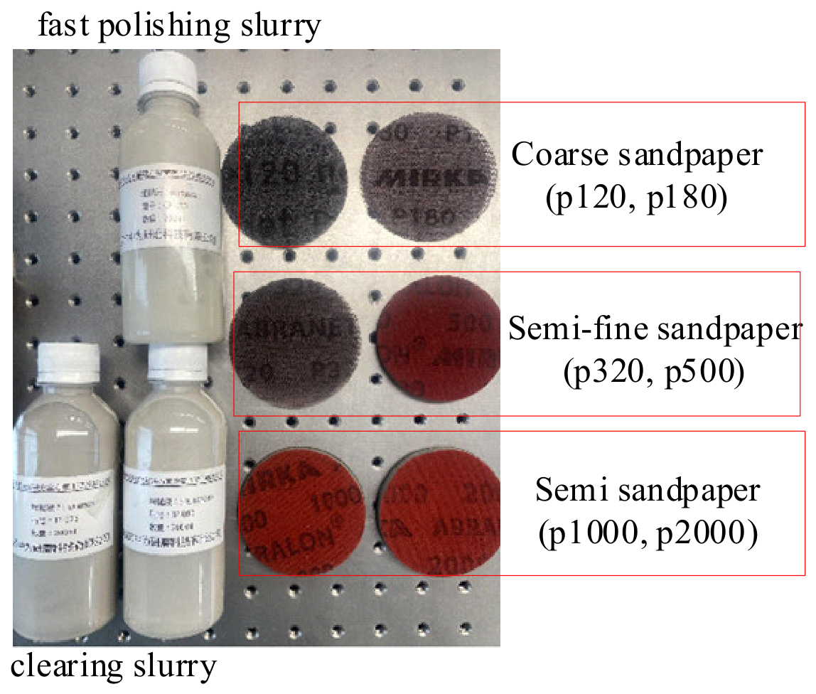
In this study, two grinding conditions were studied, plane and arc. we deliberately selected these two surfaces as benchmark cases to clearly demonstrate the effectiveness of the fuzzy adaptive strategy under controlled conditions with well-defined curvature. The arc surface already involves continuously varying contact geometry, which introduces stiffness changes along the trajectory. The grinding processes comprises multiple stages, namely rough grinding, semi-fine grinding, fine grinding, rough polishing, fine polishing. Each stage is carried out according to its specific technical requirements, and the stages follow a progressive sequence. At the end of the rough grinding stage the surface is required to be free of large scratches and collisions, with a surface roughness reaching Ra 0.8 μm. After semi-fine grinding, the surface is required to reach the basic brightness, with a surface roughness of Ra 0.4 μm. The end of the fine grinding stage requires that the surface was basically mirrored, reaching a roughness of Ra 0.1 μm. To achieve a mirror effect, a wool polishing wheel and polishing liquid were used for both rough and fine polishing. The sandpaper and polishing liquid (Mirka, Jeppo, Finland) involved were shown in Figure 15.

Figure 15. Grinding experimental supplies.

5.2. The Force and Position Tracking Effects for the Grinding Plane

To verify the effectiveness of plane force and position tracking, surface grinding experiments were conducted using the XB4 manipulator, comparing the performance of variable impedance parameters with that of constant impedance parameters. For the planar surface, Cartesian space coordinates of the grinding workpiece were collected by continuously moving the robot via the drag-teaching function, which generated sample points along the grinding path. The planned grinding trajectory was characterized by joint angle data, which can be used by the robot control system with the impedance control algorithm. Polishing experiments were performed using the force sensor and grinding head, as shown in Figure 14.

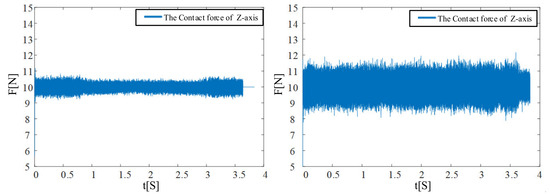
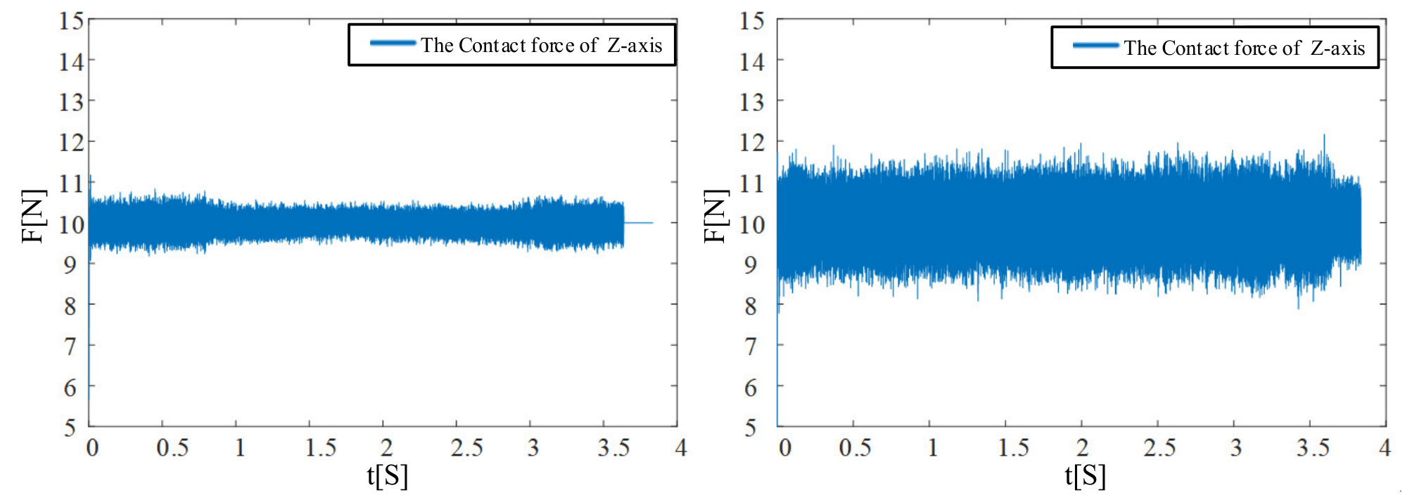
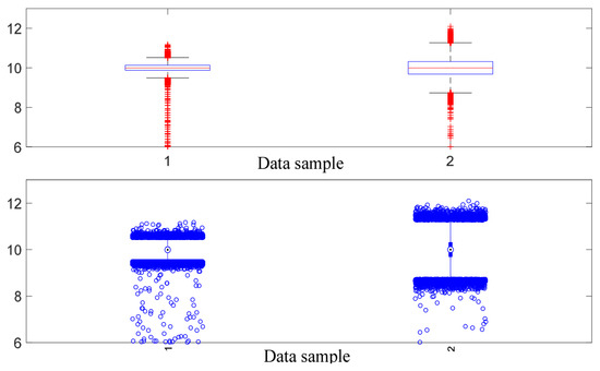
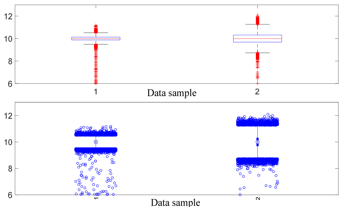
Both joint angle and the position change in Cartesian space were collected simultaneously when the grinding experiment was completed. The same trajectory was followed in both the variable- and constant-impedance experiments. Real-time grinding contact forces in the grinding process were collected through the six-dimensional force sensor, and the results are shown in Figure 16. According to the comparison diagram of the grinding contact force, the average overshoot of the variable impedance parameter is only 0.79 N, indicating a well-concentrated and low-scatter distribution of contact forces around the target value of 10 N. The average overshoot is 1.95 N after constant impedance parameter grinding experiment, and the overall overshoot effect of grinding force stability is improved by 11.6% with the variable-impedance approach. Furthermore, as depicted in the box-plot comparison and the force data (Figure 17), the variable-impedance strategy yields a more stable grinding force with a significantly smaller overshoot amplitude than the constant-impedance counterpart.

Figure 16. Comparison of plane grinding force between variable impedance and constant impedance.

Figure 17. Box comparison chart of plane grinding force.

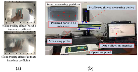
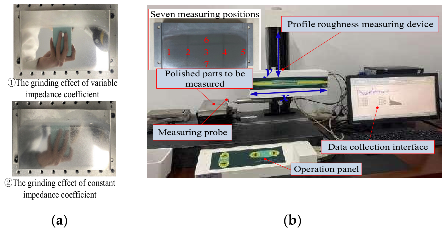
After a series of grinding and polishing processes, a comparison diagram of the grinding effect obtained with variable and constant impedance parameters is shown in Figure 18a. The polished planes were named plane 1 and plane 2. The results show that the surface finish obtained by the variable impedance control method is significantly superior to that of the conventional constant-impedance approach. In order to further characterize the advantage of the variable impedance grinding control method, the JB-5C profile roughness meter (Taiming, Shanghai, China) was used to analyze the roughness of the compared workpiece after grinding, as shown in Figure 18b.

Figure 18. Surface grinding experiment results. (a) Comparison of grinding effect between variable and constant impedance coefficient. (b) Surface roughness measurement of the polished part.

The polished workpiece was regularly divided into seven detection areas. For each area, the roughness was measured seven times, and the average values were recorded. The test results are shown in Table 4.

Table 4. Average surface roughness of the workpiece (Ra).

Sampling Location Region	1	2	3	4	5	6	7
Plane 1 Ra (μm)	0.023	0.019	0.020	0.017	0.019	0.029	0.024
Plane 2 Ra (μm)	0.048	0.045	0.032	0.037	0.045	0.048	0.043

The results show that the average surface roughness of the workpiece after grinding with the variable impedance control method is Ra 0.021 μm, whereas that obtained with the constant impedance control method is Ra 0.042 μm. According to the average roughness comparison data and the finish comparison above, it can be seen that the variable impedance control method has a greater advantage than the traditional constant impedance method in ensuring both grinding quality and consistency.

5.3. The Force and Position Tracking Effects for Grinding Arc Surface

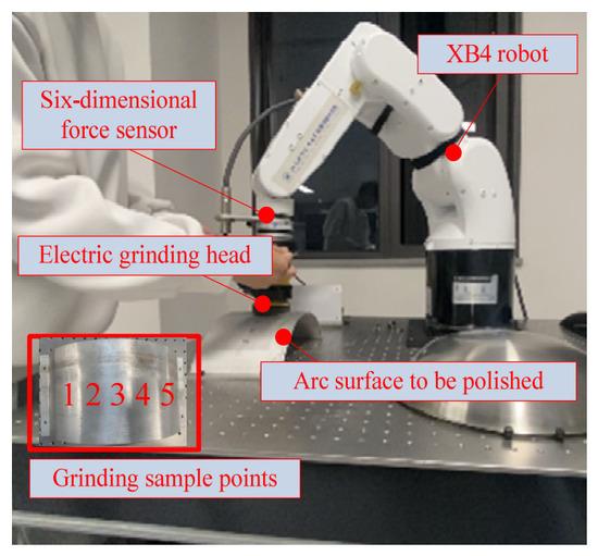
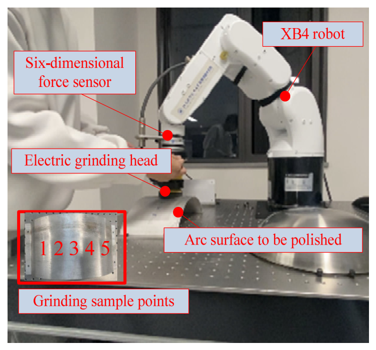
Five sample points were collected for the camber grinding parts, which were evenly distributed over the curved surface. The trajectory curve of the robot was planned through trajectory-planning function library of the control system, which interpolates and supplements points. By combining force sensor with the grinding head, a series of grinding and polishing experiments were subsequently performed, as shown in Figure 19.

Figure 19. The experiment of grinding the surface and sample collection point.

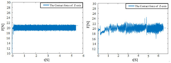
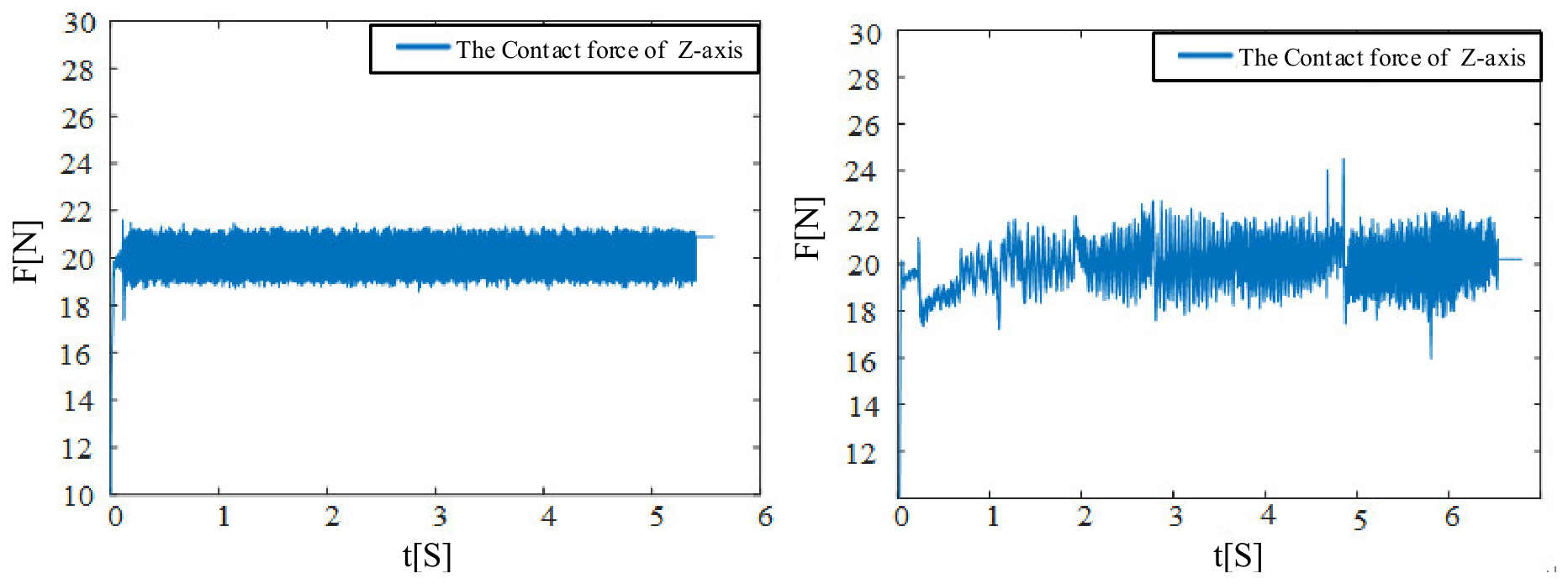
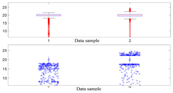
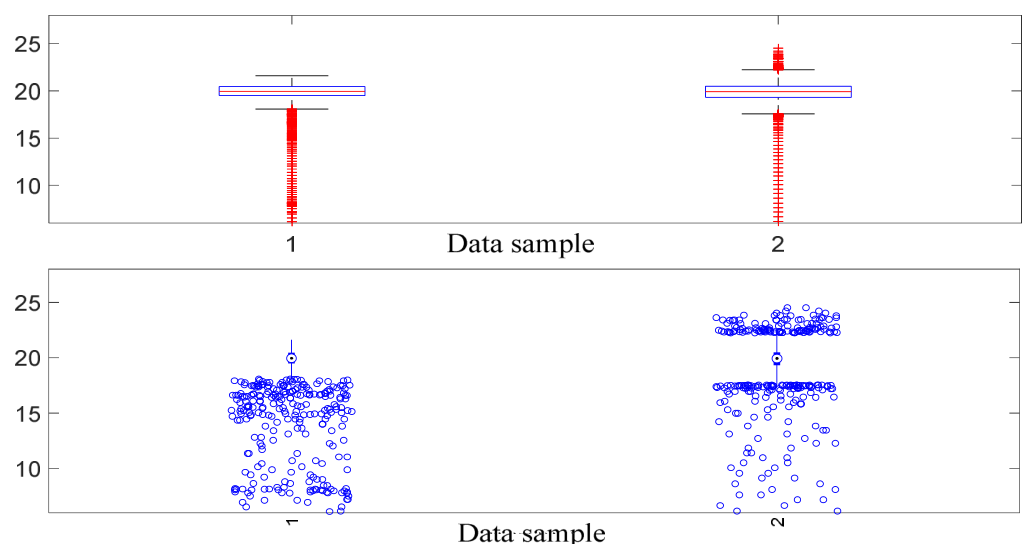
The real-time grinding contact force during the grinding process was collected through the six-dimensional force sensor, as shown in Figure 20. For the curved surface grinding under constant curvature conditions, the contact force under variable impedance remained relatively stable, without excessive shocks or fluctuations. The average overshoot in the variable impedance trial is only 1.73 N, indicating that the contact force was well concentrated around the target value of 20 N with low dispersion. In contrast, the constant-impedance experiment yielded an average overshoot of 4.22 N. Compared with the constant-impedance approach, the variable-impedance method improved the overall steady-state force stability by 12.45%. According to the box-type comparison diagram and grinding contact force data (as shown in Figure 21), the variable-impedance grinding system exhibited a faster stability tracking response and a smaller overshoot amplitude than its constant-impedance counterpart.

Figure 20. Comparison of grinding force between variable impedance and constant impedance.

Figure 21. The box comparison chart of grinding forces.

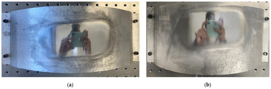
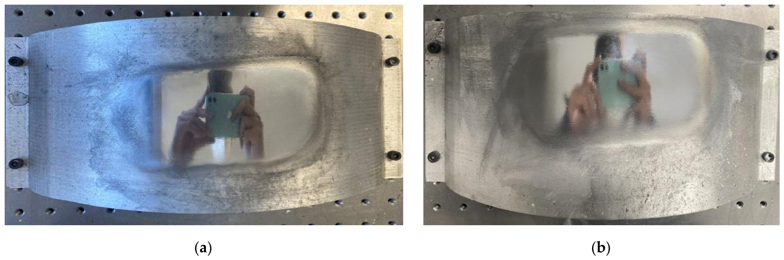
After a series of grinding and polishing processes, a comparison of the grinding effects on the curved surface obtained with variable and constant impedance parameters is shown in Figure 22. The results show that the surface finish obtained by the variable impedance control method is better than that obtained by the conventional constant impedance method.

Figure 22. A comparison of the grinding effect between the variable and constant impedance coefficients. (a) The grinding effect of the variable impedance coefficient. (b) The grinding effect of the constant impedance coefficient.

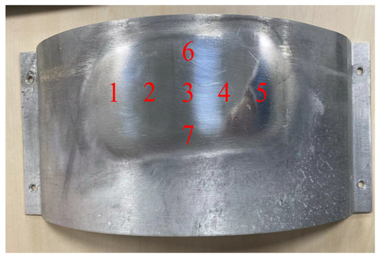
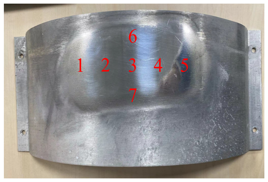
In order to further demonstrate the superiority of the variable impedance grinding control method, a JB-5C profilometer was used to measure the roughness of the polished comparative workpiece. The polished workpiece surfaces were regularly divided into seven detection areas, and the sampling points are shown in Figure 23. The detection process was repeated seven times and the average roughness in different detection areas was recorded, as shown in Table 5.

Figure 23. The area of roughness detection.

Table 5. Average surface roughness of the workpiece Ra.

Sampling Location Region	1	2	3	4	5	6	7
Plane 1 Ra (μm)	0.037	0.039	0.028	0.030	0.039	0.035	0.036
Plane 2 Ra (μm)	0.065	0.052	0.048	0.049	0.059	0.068	0.081

The results show that the average surface roughness of the workpiece ground with the variable impedance control method is Ra 0.034 μm, whereas that obtained with the constant impedance method is Ra 0.060 μm. According to the average roughness comparison data and the finish comparison above, it can be concluded that the variable impedance grinding control method has a stronger advantage than the traditional impedance in ensuring both grinding quality and consistency.

This study primarily focuses on planar and arc surfaces with relatively smooth stiffness variations; more complex free-form surfaces with abrupt stiffness changes remain to be further tested. In addition, regarding the issue that sensor noise may affect the fuzzy inference inputs, we mitigated this by applying a low-pass filter (cutoff frequency 50 Hz) to the force signal; however, in high-noise environments, more sophisticated filtering may be required. The controller parameters were tuned for the XB4 robot; different robotic platforms may require retuning, although the overall control structure remains transferable. It should be noted that a systematic experimental comparison with multiple advanced control methods on the same robotic platform remains to be conducted. This is a limitation of the current study and will be pursued in our future work, where we plan to benchmark the proposed fuzzy adaptive impedance control against learning-based and sliding-mode-based approaches under identical grinding conditions.

6. Conclusions

This paper proposes a fuzzy adaptive impedance-based force/position compliance control strategy for industrial robotic grinding. Unlike existing methods that simultaneously adjust stiffness, damping, and inertia, this work justifies, through parameter sensitivity analysis, the rationality of adjusting only the damping online, thereby avoiding oscillations caused by inertia variation and steady-state errors induced by stiffness adjustment. Moreover, a dynamic feedforward trajectory tracking controller (inner loop) is cascaded with the fuzzy adaptive impedance controller (outer loop), achieving both high-bandwidth position tracking and compliant force regulation. Experimental results show that, compared with fixed-impedance control, the proposed method reduces force overshoot by 11.6% and 12.45% for planar and curved surface grinding, respectively, and improves surface roughness from Ra 0.042 μm and Ra 0.060 μm to Ra 0.021 μm and Ra 0.034 μm, with more stable force tracking and fewer oscillations. In practice, the method is computationally efficient (running at 1 kHz in real time) and requires no prior knowledge of the environment, making it suitable for industrial polishing and grinding applications. In the future, online stiffness estimation and adaptive gain tuning will be investigated to further enhance the robustness of the proposed method under varying environmental conditions. Future work will focus on online stiffness estimation, adaptive gain tuning, and extension to free-form surfaces and different robotic platforms.

References

- Bozzi, A.; Graffione, S.; Sacile, R.; Zero, E. Dynamic mpc-based scheduling in a smart manufacturing system problem. IEEE Access 2023, 11, 141987–141996. [Google Scholar] [CrossRef] [Scilit]
- Iqdymat, A.; Stamatescu, G. Reinforcement learning of a six-DOF industrial manipulator for pick-and-place application using efficient control in warehouse management. Sustainability 2025, 17, 432. [Google Scholar] [CrossRef] [Scilit]
- Romero, S.; Valero, J.; García, A.V.; Rodríguez, C.F.; Montes, A.M.; Marín, C.; Álvarez-Martínez, D. Trajectory planning for robotic manipulators in automated palletizing: A comprehensive review. Robotics 2025, 14, 55. [Google Scholar] [CrossRef] [Scilit]
- Pitschke, E.; Schinhaerl, M.; Rascher, R.; Sperber, P.; Smith, L.; Stamp, R.; Smith, M. Simulation of a complex optical polishing process using a neural network. Robot. Comput.-Integr. Manuf. 2008, 24, 32–37. [Google Scholar] [CrossRef] [Scilit]
- Walker, D.D.; Freeman, R.; Mccavana, G.; Morton, R.; Riley, D.; Simms, J.; Brooks, D.; Kim, E.; King, A. Zeeko/UCL process for polishing large lenses and prisms. Proc. Large Lenses Prism. SPIE 2002, 4411, 106–111. [Google Scholar] [CrossRef] [Scilit]
- Zhao, X.; Zhao, H.; Chen, P.; Ding, H. Model accelerated reinforcement learning for high precision robotic assembly. Int. J. Intell. Robot. Appl. 2020, 4, 202–216. [Google Scholar] [CrossRef] [Scilit]
- Grotjahn, M.; Heimann, B. Model-based feedforward control in industrial robotics. Int. J. Robot. Res. 2002, 21, 45–60. [Google Scholar] [CrossRef] [Scilit]
- Asensio, J.; Chen, W.; Tomizuka, M. Feedforward input generation based on neural network prediction in multi-joint robots. J. Dyn. Syst. Meas. Control 2014, 136, 031002. [Google Scholar] [CrossRef] [Scilit]
- Zhang, R.; Wang, Z.; Bailey, N.; Keogh, P. Experimental assessment and feedforward control of backlash and stiction in industrial serial robots for low-speed operations. Int. J. Comput. Integr. Manuf. 2023, 36, 393–410. [Google Scholar] [CrossRef] [Scilit]
- Hamad, M.; Karayiannidis, Y. Modelling and Feed-Forward Control of Robot Arms with Flexible Joints and Flexible Links. Master’s Thesis, Chalmers University of Technology, Gothenburg, Sweden, 2016. [Google Scholar]
- Pfanne, M.; Chalon, M.; Stulp, F.; Ritter, H.; Albu-Schäffer, A. Object-level impedance control for dexterous in-hand manipulation. IEEE Robot. Autom. Lett. 2020, 5, 2987–2994. [Google Scholar] [CrossRef] [Scilit]
- Seraji, H.; Howard, A. Behavior-based robot navigation on challenging terrain: A fuzzy logic approach. IEEE Trans. Robot. Autom. 2002, 18, 308–321. [Google Scholar] [CrossRef] [Scilit]
- Xu, G.; Chen, W.; Gao, X.; Song, A. Robot-aided resistance training method based on impedance identification and hybrid control. J. Mech. Eng. 2016, 52, 8–14. [Google Scholar] [CrossRef] [Scilit]
- Xing, H.; Ding, L.; Gao, H.; Xia, K.; Liu, Z.; Tao, J.; Deng, Z. Adaptive tracking of axial position for valve-turning with a robot based on impedance control. J. Mech. Eng. 2019, 55, 124–134. [Google Scholar] [CrossRef] [Scilit]
- Zahedi, F.; Chang, D.; Lee, H. User-adaptive variable damping control using Bayesian optimization to enhance physical human-robot interaction. IEEE Robot. Autom. Lett. 2022, 7, 2724–2731. [Google Scholar] [CrossRef] [Scilit]
- Gui, K.; Tan, U.X.; Liu, H.; Zhang, D. A new impedance controller based on nonlinear model reference adaptive control for exoskeleton systems. Int. J. Humanoid Robot. 2019, 16, 1950020. [Google Scholar] [CrossRef] [Scilit]
- Zhang, X.; Khamesee, M.B. Adaptive force tracking control of a magnetically navigated microrobot in uncertain environment. IEEE/ASME Trans. Mechatron. 2017, 22, 1644–1651. [Google Scholar] [CrossRef] [Scilit]
- Zhang, Y.; Wu, Q.; Chen, B.; Wu, H.; Liu, H. Fuzzy neural network impedance control of soft lower limb rehabilitation exoskeleton robot. Robot 2020, 42, 477–484. [Google Scholar]
- Luo, J.; Solowjow, E.; Wen, C.; Ojea, J.A.; Agogino, A.M.; Tamar, A.; Abbeel, P. Reinforcement learning on variable impedance controller for high-precision robotic assembly. In Proceedings of the 2019 International Conference on Robotics and Automation (ICRA); IEEE: Piscataway, NJ, USA, 2019; pp. 3080–3087. [Google Scholar]
- Yang, C.; Peng, G.; Cheng, L.; Na, J.; Li, Z. Force sensorless admittance control for teleoperation of uncertain robot manipulator using neural networks. IEEE Trans. Syst. Man. Cybern. Syst. 2021, 51, 3282–3292. [Google Scholar] [CrossRef] [Scilit]
- Ren, T.; Dong, Y.; Wu, D.; Chen, K. Impedance control of collaborative robots based on joint torque servo with active disturbance rejection. Ind. Robot Int. J. Robot. Res. Appl. 2019, 46, 518–528. [Google Scholar] [CrossRef] [Scilit]
- Li, Z.; Zhou, Y.; Wang, L.; Zhang, X.; Li, A.; Zhu, M.; Wu, Q. An end-to-end controller with image-based visual servoing of industrial manipulators with soft-actor-critic algorithm. Knowl.-Based Syst. 2025, 311, 112980. [Google Scholar] [CrossRef] [Scilit]
- Hu, Y.S.; Yan, H.C.; Zhang, H.; Wang, M.; Zeng, L. Robust Adaptive Fixed-Time Sliding-Mode Control for Uncertain Robotic Systems with Input Saturation. IEEE Trans. Cybern. 2023, 53, 2636–2646. [Google Scholar] [CrossRef] [Scilit] [PubMed]
- Kang, H.J. Precision Tracking of Industrial Manipulators via Adaptive Nonsingular Fixed-Time Sliding Mode Control. Mathematics 2025, 13, 2641. [Google Scholar] [CrossRef] [Scilit]
- Liu, Z.; Zhang, O.; Gao, Y.; Zhao, Y.; Sun, Y.; Liu, J. Adaptive Neural Network-Based Fixed-Time Control for Trajectory Tracking of Robotic Systems. IEEE Trans. Circuits Syst. II Express Briefs 2023, 70, 241–245. [Google Scholar] [CrossRef] [Scilit]
- Jing, Y.; Gao, W.; Han, Z.; Hu, M. Dynamics Modeling and Multi-condition Analysis for 6-DOF Industrial Manipulator. In Proceedings of the International Conference on Intelligent Robotics and Applications; Springer: Berlin/Heidelberg, Germany, 2021; pp. 602–610. [Google Scholar]
- Ni, T.; Xu, H.; Li, D.; Zhang, H. Research on dynamics feedforward compliance control of 6-DOF platforms. China Mech. Eng. 2022, 33, 683–689. [Google Scholar]
- Nazmara, G.; Fateh, M.M.; Ahmadi, S.M. A model-reference impedance control of robot manipulators using an adaptive fuzzy uncertainty estimator. Int. J. Comput. Intell. Syst. 2018, 11, 979–990. [Google Scholar] [CrossRef] [Scilit]
Disclaimer/Publisher’s Note: The statements, opinions and data contained in all publications are solely those of the individual author(s) and contributor(s) and not of MDPI and/or the editor(s). MDPI and/or the editor(s) disclaim responsibility for any injury to people or property resulting from any ideas, methods, instructions or products referred to in the content. |
© 2026 by the authors. Licensee MDPI, Basel, Switzerland. This article is an open access article distributed under the terms and conditions of the Creative Commons Attribution (CC BY) license.