


Abstract
Synthetic data generation is a potential solution for addressing limited data in manufacturing defect detection. In injection molding of automotive tubes, surface defects such as splay present as white or silver streaks in the tube’s texture, that are difficult to capture in sufficient quantity for training robust object detection models. This study proposes Fast-DG2GAN: a DG2GAN based, computationally optimized, generative style defect generator for manufacturing defect images. Fast-DG2GAN achieves a 56% reduction in training time relative to the original DG2GAN, completing training in 334.9 min compared to 768.0 min, while maintaining comparable image quality metrics with a best FID score of 132.83 and IS 1.45 ± 0.08. Key contributions to this DG2GAN variant include depth-wise separable convolutions, reduced residual blocks, and automatic mixed precision (AMP) training, to improve training time. Training stabilization techniques include perceptual loss, feature matching, and exponential moving average of weights (EMA). Legacy Generative Adversarial Network (GAN) architectures are benchmarked for feasibility and include WGAN, DCGAN, and FastGAN, for fine-grained defect image generation essential to downstream object detection. Metrics, such as Inception Score (IS) and Fréchet Inception Distance (FID) are used for quantitative performance evaluation. This study highlights the potential of GAN-generated datasets to augment real-world training for defect detection models.
1. Introduction
Selecting an appropriate GAN (Generative Adversarial Network) variant for the purpose of generating images of parts with defects is crucial, as a robust dataset is needed for successful object detection deployment. This study proposes Fast-DG2GAN, a computationally optimized variant of the Dual-Generator GAN (DG2GAN) [1], as a novel solution to scarce sample data in object detection applications in the manufacturing industry. Fast-DG2GAN achieves a 56% reduction in model training time relative to the original DG2GAN through depth-wise convolutional separations, a reduction in residual blocks, and automatic mixed precision (AMP) training, while maintaining statistically comparable image quality metrics. This study compares GAN model performance, where a limited number of samples (five samples) are supplied as the basis to build an object detection program, for inline defect detection in a manufacturing setting. A method is required to generate a dataset of defect images where an object detection model could be successfully trained.
GANs work based on two separate neural networks that are trained by an adversarial process. The generator produces an image based on noise, and the discriminator decides if the image produced by the generator is “real” or “fake”. The figure (Figure 1) below shows the basic process [2].
Figure 1.
Example of generator–discriminator process [2].
During the training process, the generator starts with producing noise or basic geometry. As the discriminator can easily tell the image is fake, it forces the generator to produce better images. This happens over many attempts or iterations until the generator is able to “fool” the discriminator with a “fake” image [2], see Figure 2.
Figure 2.
Example of generator output images [2].
Utilizing a GAN will help build a dataset suitable for object detection model training. There are dozens of GAN architectures and variants available for potential use [3]. Several model architectures and variants are suitable for the use case of limited samples. This study will benchmark three legacy GAN types for feasibility in industrial applications; The Wasserstein GAN (WGAN), Deep Convolutional GAN (DCGAN), and Free Adversarial Training GAN (FastGAN). The original Dual-Generator GAN (DG2GAN) will be evaluated along with the proposed Fast-DG2GAN variant as a baseline to substantiate the novel method. The GAN variants provide a path for transforming sparse datasets into meaningful data for use with an object detection application.
Some of the benefits to these types of GANs include unsupervised image synthesis, avoidance of model collapse, high resolution outputs, and the ability to generate images based on limited size datasets [3]. The difficulties when training these GANs are that extensive hyperparameter tuning is required, along with pre-data augmentation. Training stability, model collapse and vanishing or exploding gradients are common challenges when tuning a GAN [4].
This study explores the benefits and difficulties in selected GAN architectures and variants that are suitable for limited data and provides a path forward with a novel framework, Fast-DG2GAN, for further improving synthetic defect image generation through computational efficiency and training stabilization.
2. Related Research
2.1. GAN Introduction
The foundational basis of GANs is that they consist of two neural networks, a generator and a discriminator. The generator is responsible for the synthetic creation of images from noise and the discriminator’s function is to differentiate between “real” and “fake” images. The two neural networks compete, whereas the generator tries to “fool” the discriminator by synthetically creating images that look to be real. The discriminator tries to differentiate between real images provided and synthetic images generated [5]. The figure below (Figure 3) illustrates the GAN flow [6].
Figure 3.
Original GAN process flow [6].
The discriminator returns the probability that an image is real. The generator tries to minimize the loss, making the discriminator assign higher probabilities to synthetic images [5]. Please see Equation (1) below [5]:
GANs have many applications such as image synthesis, domain adaptation, and learning. There are a few main challenges in successful GAN applications including mode collapse, training instability and evaluation [4,5]. Mode collapse is present when some features of images are ignored, and the diversity of features is lacking. This can be due to overfitting discriminator feedback, where the generator consistently fools the discriminator. Additionally, the discriminator may not be able to detect the lacking diversity from the generator [6]. Because there is competition between the generator and the discriminator, the training is difficult due to divergence, oscillations, and the inability to converge on a solution. If not tuned correctly, the updates to both networks in parallel can destabilize the training process [6]. Due to the lack of standard evaluation methods for GANs, some of the ways to evaluate may not fully capture the quality and diversity of generated samples [6]. Evaluation tools such as the Inception Score (IS) and Fréchet Inception Distance (FID) have limitations surrounding choice of pre-trained models and assessing high-dimensional data [7].
GANs have a wide range of applications and functionality. There are dozens of GAN architectures and their variants that can be applied for synthetic image generation [6]. Select GAN architectures or GAN variants are identified for feasibility on images with manufacturing defects and considering scarce or limited dataset availability. Select GANs are considered for the purpose of scarce or limited datasets featuring product defects, noting that there are several more that could also be considered. Five GANs were selected for related research including Vanilla GAN, Wasserstein GAN (WGAN), Deep Convolutional GAN (DCGAN), and FastGAN. Legacy GANs chosen for testing and experimentation on the splay defects on injected molded shock cover tubes include the Wasserstein GAN (WGAN), Deep Convolutional GAN (DCGAN), and FastGAN.
2.2. Vanilla GAN
Vanilla GAN is a term to describe the original GAN architecture proposed by Goodfellow, without major refinements [5]. The original GAN architectures have three main challenges: mode collapse, training instability, and gradient vanishing. See Figure 4 below for the dataflow for Vanilla GAN [7].
Figure 4.
Vanilla GAN dataflow [7].
Mode collapse occurs when the generator produces a limited number of features, not being able to capture the full distribution of the data [8]. This happens when the generator finds outputs that always “fool” the generator, leading to limited variability in generated images [6]. In training instability, the loss function for the discriminator can oscillate or diverge during the training process [9]. The minmax optimization causes the non-convex form of instability during training [6]. Vanishing gradients occur when the discriminator is too strong, and with reduced gradients, the generator has difficulty learning [9]. The discriminator consistently “wins” the game, leaving the generator with small gradients [6]. The mode collapse example below is in Figure 5 [8].
Figure 5.
Mode collapse example [8].
The original GAN or Vanilla GAN serves as the underlying foundation of how GANs function. But, based on the Vanilla GAN several developments were inspired such as WGANs, Conditional GANs (CGANs), and Deep Convolutional GANs (DCGANs). All of these improvements with new architectures or variants all aim to alleviate the challenges and limitations that the original Vanilla GAN is susceptible to [8]. Improvements to Vanilla GAN are made through architecture improvements, and other techniques such as improved loss functions, regularization techniques, and transfer learning [6].
2.3. Wasserstein GAN (WGAN)
Basic or traditional GANs utilize the Jensen–Shannon divergence to evaluate the difference between the discriminator’s distribution and the data distribution [9]. There are a number of issues with training GANs, including training instability, mode collapse, hyper parameter sensitivity, and vanishing gradients. Researchers are continuously producing new architectures and variants to address GAN training issues [3,6]. WGAN aims to resolve training instability, mode collapse, and gradient vanishing. WGAN replaces the Jensen–Shannon divergence with the Wasserstein distance algorithm, the key difference being that the Wasserstein distance calculation does not saturate, and supports better gradients, as shown in Figure 6 [9].
Figure 6.
Wasserstein distance visualization [9].
The Wasserstein distance works by taking two distributions, one being the real data, and the other being the generator’s data. It measures the minimum work required to transform the real data into the generator data [9]. Equation (2) below, shows the Wasserstein distance calculation [9].
WGAN works by the discriminator estimating the Wasserstein distance between the distribution of the real data and generator data. With the discriminator being optimized to apply the Wasserstein distance and to satisfy the Lipschitz continuity, the discriminator’s weights are clipped [9]. WGAN aims to avoid mode collapse, improve training stability, and achieve better convergence by minimizing the difference between two distributions [9]. Importantly, even though WGAN improves convergence and reduces mode collapse and instability, these training failure modes are still present. Additional research shows improved WGAN architectures that try to resolve issues with the original WGAN [10]. For example, Sobolev WGAN (SWGAN) improves stability and convergence by implementing the Sobolev duality which has smoother derivative constraints and broad function space, which makes for more robust training [10].
2.4. Deep Convolutional GAN (DCGAN)
Deep Convolutional GANs (DCGAN) utilize a structure by means of convolutional layers for the purpose of generating quality images. With unlabeled data, training stability is improved while leveraging unsupervised learning [11]. Convolutional layers replace connected layers in both the generator and discriminator’s architecture. Strided convolutions replace pooling layers in the discriminator and fraction-strided layers are used in the generator [11]. Batch normalization is used in both the generator and discriminator network to improve training stabilization. The ReLU activation function is used in the generator, with the exception of the output layer utilizing the tanh function. The discriminator uses the Leaky ReLU activation function [11]. See Figure 7 below for the DCGAN architecture.
Figure 7.
DCGAN architecture example [11].
DCGAN uses an unsupervised feature learning approach. The DCGAN layers in the discriminator can learn visual features without need for supervision. Another benefit is that the learned features, with some fine-tuning, can be applied to image classifications [11]. Although improvement is made with DCGAN, there are limitations in practical use. Mode collapse is still likely with the difficulty capturing fine details in images. The overall performance of a DCGAN model is very dependent on dataset diversity and parameter adjustments [11].
2.5. FastGAN
Free Adversarial Training GAN (FastGAN) was introduced with the purpose of addressing the issue of slow training and generated image quality. The architecture in FastGAN is designed to be lightweight for both the generator and the discriminator with results showing reduced mode collapse, improved training stability, and better image quality [12]. FastGAN is able to decrease training time and produce better quality images compared to VanillaGAN, while reducing computational resources, due to reduced complexity in both the discriminator and generator’s model architecture [13].
In FastGAN, there are several architecture and function improvements. FastGAN uses a ResNet-based generator and discriminator without complicated activation functions, such as self-attention or spectral normalization [12]. FastGAN modifies the discriminator’s loss function to have a hinge loss component that replaces binary cross-entropy, as it reduces instability and gradient vanishing. A KL-divergence regularization is added to increase diversity within classes in the generator output [12].
Even with the improvements made with FastGAN, there are a few limitations. The resultant images or artifacts may have some unwanted patterns or leave a “checkerboard” effect over the image. This effect can be noticed where finer details should exist on the image [13]. Sometimes images can lack sharpness and texture detail, especially in images where detail should vary. Mode collapse is possible where there is a lack of diversity in generated images and redundancy in generated images. This is more evident in limited datasets [13].
2.6. DG2GAN
In 2024, Deng et al. proposed DG2GAN (Dual-Generator Dual-Discriminator GAN) as a novel framework for generating high quality images with defects to improve defect recognition in Resnet object detection models [1]. The aim was to improve industrial object detection with defect generation to address imbalanced datasets, as traditional augmentation techniques failed to capture the fine-grained details of real defects [1]. Figure 8 shows the dual-generator, quad-discriminator flow [1].
Figure 8.
Architecture of the DG2GAN, which contains six networks: two generators and four discriminators. The objective of DG2GAN includes DG2 adversarial loss, cycle consistency loss, and DJS [1].
DG2GAN improves traditional issues with cycle consistency loss and a 4-discriminator strategy. The architecture for this model utilizes 2 generators: one to construct clean (defect free) images from defect images, and the second to construct defect images from clean (defect free) images. Four discriminators, in complimentary pairs, act at various levels to produce increased fidelity and increased diversity. The first pair (D1n, D1d) are in the conventional position of judging realism in generated images. The second pair (D2n, D2d), promote diversity by having the generator produce results that fall outside the real distribution, thereby producing outputs further away from repetitive artifacts [1]. Figure 8 illustrates the design and data flow of the original DG2GAN architecture.
The authors introduce a DJS-Loss (Jenson–Shannon divergence) and DG2 adversarial loss, that work in tandem to encourage the generators to produce images that are varied and realistic, without repetitive patterns being observed [1]. DJS-Loss is utilized as a suppletory optimization for the D2n and D2d discriminators, thus making the loss function flexible to data distribution, while observing performance improvement. Please see Equation (3) for DJS optimized loss [1].
DG2GAN defect detection accuracy was improved from 86.9% to 94.6% and average precision from 59.8% to 80.2% when benchmarked against WGAN, D2GAN, and CycleGAN architectures trained on the same dataset [1]. Fréchet Inception Distance (FID) and visual grading confirm the DG2GAN produces sharper images with fewer artifacts generating more authentic defects. DG2GAN is valuable for industrial applications as it can encourage adequate dataset generation when defect samples are limited or costly to collect.
3. Methods
3.1. Background
For experimentation and work towards practical industrial applications, images of injection molded tubes were obtained. These images contain a defect in the injection molding process where splay is present. Splay is a cosmetic defect that appears as silver or off-white spots and streaks on the surface of the plastic tube. Splay occurs when moisture turns to steam and gets trapped within the molded part. Splay can be caused by other gases that trap air. The image below (Figure 9) is an example of splay occurring on the surface of the part, and an example of a defect free part.
Figure 9.
Example of splay defect on injection molded tube (Left). Example of defect-free tube (Right).
The dataset is based on limited samples. There were 5 unique parts with splay defects and images were obtained with the splay defect visible during different degrees of rotation. In total, there was a limited dataset of 25 images containing the injection mold splay defect.
A working GAN is needed to artificially generate a dataset of thousands of images that can be used to train a model in an object detection application where splay is detected on production parts. This work explores elementary GAN architectures and variants with the goal of, while working with scarce or limited data, finding a path forward towards a working GAN solution that can generate splay defects on new images.
This work explores select legacy GAN types and variants that, based on research, may be suitable for data that is limited in nature. Each GAN experiment for splay defects explores the same level of image data augmentation and GAN specific hyperparameter tuning. The novel Fast-DG2GAN is benchmarked against the original DG2GAN to highlight training speed and image quality improvements. Loss plots are generated for each experiment to compare results and aid in the determination of mode collapse and the model’s ability to capture fine details. Ultimately, results of synthetic defect images that best resemble real defect images are paramount for judging overall success along with FID and IS. FID and IS are interpreted as directional rather than statistically precise and complement actual generated image results. For each experiment, results are discussed, and future work or modifications are suggested as next steps.
3.2. GAN Dataset Generation
The dataset for training all GAN models was assembled using 25 source images from each class: 5 defect sample parts, and 5 good sample parts. Brightness, saturation, and scale augmentations were applied to generate the dataset of 100 defect samples and 100 good samples needed for training the sample GAN models, see Figure 10.
Figure 10.
Dataset augmentation to original images example.
This dataset of 200 augmented images with original images were used for all GAN model training experiments. The exceptions were WGAN and FastGAN that only used defect images and not clean images. The purpose is to meet the minimum required images for training datasets with limited data (around 100 images) and provide some data variation with noise and scaled images.
3.3. Experimental Method
This study proposes Fast-DG2GAN, a modified and improved version of the DG2GAN by Deng et al. This novel GAN utilizes the dual-generator and discriminator method by Deng et al. and implements several improvements to reduce training time while maintaining or improving image generation quality. Generator architectural changes were made, such as depth-wise separable convolutions used in place of Conv2d and reduced residual blocks to improve efficiency and reduce computational overhead. Automatic mixed precision (AMP) is used to split functions between F16 and F32 instead of using F32 across all functions, thus providing improved computation efficiency. The discriminators are updated using image pooling, a technique borrowed from CycleGAN to stabilize discriminator updates. Perceptual loss (VGG) is implemented to aid in real-time style transfer and improve image resolution. Feature matching is implemented to aid in training stabilization. Lastly, exponential moving average of weights (EMA) is used to stabilize training curves by reducing noise. Figure 11 displays a pipeline from the original dataset to a dataset augmented with synthetic images.
Figure 11.
Proposed Fast-DG2GAN pipeline from the original dataset to a dataset augmented with synthetic images.
All experiments were conducted on a Lenovo ThinkStation P330 desktop workstation running Windows 11 Pro, equipped with an Intel Core i7-8700 CPU (3.20 GHz, 6 cores, 12 logical processors), 64 GB of RAM, and an NVIDIA GeForce RTX 3060 GPU (1 GB dedicated VRAM). All five architectures were trained under identical hardware conditions to ensure a fair comparison of training time across experiments.
3.4. Fast-DG2GAN Generator Architecture
The modified generator for Fast-DG2GAN utilizes an encoder–residual–decoder system which is used in image-to-image translation and implements depth-wise separable convolutions to reduce computational overhead while maintaining the overall network architecture of the original DG2GAN. Figure 12 shows the proposed Fast-DG2GAN network.
Figure 12.
Proposed Fast-DG2GAN design.
Typical convolution layers combine model cross-channel and spatial correlations, which can be computationally demanding with high image resolutions. Depth-wise separable convolutions split the operations into two stages: a depth-wise spatial convolution to each channel, then a pointwise convolution for inter-channel functions. This leads to more effective parameter utilization and computational efficiency [14]. Chollet showed computational efficiency improvements with Xception being more accurate than Inception V3 with fewer parameters, which can be correlated to architectural function rather than model size [14].
The original DG2GAN architecture utilizes residual blocks for batch normalization [1]. The encoder–residual–decoder method comes from Cycle-GAN architectures, which were intended for complex image translation operations. Recent research indicates increasing the residual depth affects network optimization. Deeper residual networks increasingly influence forward and backward variance as residual depth increases [15]. Fast-DG2GAN reduces the number of residual blocks in the residual stage of the generator architecture from 12 (Original DG2GAN) to 4 (Fast-DG2GAN). The reduction reflects the reduced complexity in typical manufacturing defects vs. Cycle-GAN design intent as appearance transformations are minimal. In practice, the image quality and FID/IS between the original DG2GAN and Fast-DG2GAN did not justify additional residual blocks, thus improving computational efficiency. Figure 12 shows the proposed Fast-DG2GAN design.
3.4.1. Automatic Mixed Precision (AMP)
Kuchaiev et al. (2018) proved that deep neural networks can utilize training with FP16 arithmetic without accuracy loss, when combined with FP 32 weight masters, loss scaling, and FP16 to FP32 pooling in matrix multiplications [16]. Fast-DG2GAN employs automatic mixed precision (AMP) training to reduce GPU memory usage. AMP trains using FP16 weights for gradients and activations, while holding FP32 master weights for the optimizer function [16]. AMP mixed precision training addresses one of the instability problems, where approximately 5% of weight gradient values have exponents less than −24, which would translate to zero in FP16 optimizer when multiplied by the learning rate, which has an unfavorable effect on the training model [16]. AMP utilizes FP16 for forward and backward passes and selective use of FP32 operations. Without AMP, most operations occur through FP32 [16]. Loss scaling is achieved by scaling up before the backpropagation, allowing small factor gradients to be held within FP16 dynamic range, then upscaled before the optimizer operation [16].
Computationally intensive operations in reduced precision with precision necessitated operations in FP32 can extend across hardware and model configurations [17]. Back-propagated gradient values are shifted into the FP16 representable range and the negative exponent gradient values are captured for accuracy, as scaling is inherent with representations of fixed points, making it more accurate for deep learning training runs [17].
3.4.2. Image Pooling
Due to common training difficulties in GANs, training instability can occur when the discriminator overfits to recent generated images and adapts to the most recent generated outputs, thus causing training oscillation [18]. Due to the discriminator model focusing on recent images, there is a lack of memory. This memory restriction may cause training instability and cause the refiner network to reintroduce artifacts that the discriminator lost memory on [18]. Images generated throughout the adversarial training process represent samples from the model distribution. Therefore, they constitute synthetic samples to feed the discriminator. Limiting discriminator updates to most recent image outputs may result in forgetting earlier failure modes. Thus, the discriminator should hold discriminative capacity over current and previously generated images [19]. To address training instability, discriminator updates are computed over a replay buffer of previously generated images instead of the current batch of images. At each epoch, half of the discriminator batch is used from the current generator, and the other half is sampled from a random fixed-sized buffer. The buffer updates by randomly replacing entries with new generated images [18]. Shrivastava et al. demonstrated a 56% increase in task error when the buffer was removed, and since has adopted image pooling as standard practice for image-to-image pipelines [18].
To mitigate the adverse training effect, our method for aiding in reducing training oscillation is image pooling. Discriminators are updated using a rolling pool (buffer) of 50 previously generated images to improve training stability [19]. Fast-DG2GAN bridges synthetic manufacturing defect images to real defect images. The same adaptation challenges exist that image pooling mitigates. The image buffer ensures that the discriminator maintains a broad range of what consists of a generated image across the training run.
3.4.3. Perceptual Loss (VGG)
The DG2GAN generator is trained using a perceptual loss function formulated in the feature space of the pre-trained network, instead of in the pixel space. Per-pixel losses such as MSE move the generator toward pixel-wise averages of possible outputs, producing smooth, perceptually unconvincing images. Rather, based on Johnson et al., we compute the content loss as the Euclidean distance between intermediate activations of a static VGG network, applied to target and generated images [20]. This method ensures the generator matches high level semantic and texture-based structure instead of pixel values [20]. As proposed by Ledig et al. in super resolution, combining perceptual VGG content loss with adversarial loss components produces photo-realistic results that outperform MSE trained networks in perception quality, given pixel level metrics being lower [21]. Zhang et al. empirically confirmed the need for feature loss, as their ablation study shows replacing VGG feature loss with color-space L1 causes a significant reduction in output quality, with SSIM lowering from 0.853 to 0.683 [22].
3.4.4. Feature Matching
This study implements training of the network with feature matching, as used by Salimans et al. Feature matching is utilized to stabilize training by replacing the adversarial objective with a distributional matching constant [23]. In standard GAN training, the generator is encouraged to maximize the discriminator output, which can become unstable as the generator overtrains on discriminator outputs. Feature matching mitigates training instability by training the generator to match the expected feature statistics of real images [23]:
where is the activation at an intermediate discriminator layer, see Equation (4). The discriminator is trained without feature matching modification. As the discriminator is adversarially trained to find the most discriminative features of image data, the feature space is semantically adaptive, therefore, the generator is skewed toward matching distributional structure [23].
Mroueh et al. showed that mean feature matching minimizes defined statistical distance between real and generated distributions [24]. They situate integral probability metric (IPM) feature matching in the same family as Wasserstein GAN, which the loss provides a sample that correlates to image quality, the distribution matches the expected feature statistics and stabilized gradient flow [24]. Yang et al. deployed feature matching as a style consistency loss in GP-UNIT, where the channel-wise mean of the discriminator’s intermediate features attributes to style similarity [25]. Yang et al. were able to demonstrate that discriminator feature matching is sufficient for distributional alignment in translation settings without additional cycle constraints [25]. The total generator loss in Fast-DG2GAN is a weighted combination of losses (DJS loss, cycle-consistency loss, Perceptual VGG, adversarial loss, feature matching, and identity loss). Formula 5 below shows the combined generator loss:
3.4.5. Exponential Moving Average of Weights (EMA)
To continue with training stabilization of the generator techniques, we maintain an exponential moving average (EMA) of the generator weights throughout the training process. Following seminal work from Polyak and Juditsky, who empirically proved that averaging iterations of stochastic approximation achieves the theoretical optimal convergence rate without knowing the loss history curvature, we apply an EMA update throughout the training loop [26]:
where are the generator weights at epoch t and is the decay factor [26], see Equation (6). By nature of GANs, substantial stochastic noise from gradient updates is introduced between the generator and discriminator. By utilizing EMA, it absorbs the noise to produce a high-quality weight estimate than what a single iteration provides [26]. Research from Morales–Brotons et al. provides empirical validation of EMA use in deep learning, proving that EMA consistently outperforms last-iteration solutions of generalization across multiple architectures and datasets, and explicitly states that EMA has been studied in the minimax optimization algorithm [27]. They show that the EMA solution is qualitatively different from the SGD last-iteration, thus averaging with higher learning rates invokes implicit regularization that encourages learning of more general representations [27]. In our Fast-DG2GAN context, EMA promotes more distributionally consistent synthetically generated images. We set = 0.999 and maintain the EMA outside of the training loop so that there are no inter-optimizer dynamic effects. We use EMA exclusively for inference and evaluation, as it is not applied to the loss equation.
4. Experiments and Results
4.1. Fast-DG2GAN
The proposed Fast-DG2GAN framework was tested in five experiments for parameter tuning comparison, to optimize results. In total, 512 × 512 input images were used for the network, consisting of 100 clean tube images and 100 splay defect images on the tubes.
The generator model borrows an encoder–residual–decoder framework from the original DG2GAN work [1]. Depth-wise separable convolutions are used to expand the input image to 64 channels (7 × 7, s = 1, p = 3), followed by instance normalization and ReLU. Two downstream depth-wise separable down-sampling stages (3 × 3, s = 2, p = 1) progressively expand the channel dimensions to 128 and 256 while reducing the spatial resolution. Each block is followed by instance normalization and ReLU, producing a representation at 256 × 128 × 128. Four residual blocks are used in Fast-DG2GAN and are applied at this resolution, each consisting of two depth-wise separable convolutions (3 × 3, p = 1) with instance normalization and ReLU after the first convolution, and instance normalization after the second convolution, with input added to the block output as a skip connection. The decoder mirrors the encoder using two transposed convolutions (3 × 3, s = 2, p = 1) to up-sample through 128 and 64 channels at progressive spatial resolutions, each followed by instance normalization and ReLU. A final convolution (7 × 7, s = 1, p = 3) maps the features back to the output channels with a tanh activation normalizing pixel values. Depth-wise separable convolutions are used in Fast-DG2GAN to aid in reducing computational overhead [14], see Figure 13.
Figure 13.
Fast-DG2GAN generator network architecture diagram.
The discriminator model inherits the framework from the original DG2GAN work, which employs a PatchGAN style discriminator [1]. Rather than producing a single scalar real or fake prediction, PatchGAN discriminators output a spatial map where each value corresponds to the authenticity of a local patch in the image. The discriminator, borrowed from DG2GAN, consists of five convolutional stages. The first layer (Conv1) maps the input image to 64 (4 × 4, s = 2, p = 1) followed by LeakyReLU (0.2), with no normalization applied. Two downstream down-sampling layers (Conv2, Conv3) double the channel dimensions to 128 and 256, respectively, using the same strided convolution configuration, each followed by instance normalization and LeakyReLU (0.2). Conv4 expands to 512 channels (4 × 4, s = 1, p = 1) with instance normalization and LeakyReLU (0.2), reducing the spatial stride to avoid excessive down-sampling. The final stage, Conv5, maps the 512-channel feature map to a single-channel output (4 × 4, s = 1, p = 1) with no activation, producing Patch-wise style maps used during adversarial training, see Figure 14.
Figure 14.
Fast-DG2GAN discriminator network architecture.
Experiment runs for the proposed Fast-DG2GAN have different hyperparameter settings to push performance metrics. Parameters evolve as training loss protocols (discussed in Section 3) are applied. Table 1 below summarizes the hyperparameters used for each run. The first run utilized parameters based on some initial trial and error. Run 2 sees the DJS change from 0.1 to 0.08, cycle loss change from 10 to 8.5, and perceptual loss change from 0.9 to 0.58. The FID and IS slightly degraded with this run. Experiment 3 for Fast-DG2GAN had a learning rate of 0.00015 and increased the cycle loss from 8.5 to 9 and perceptual loss from 0.58 to 0.6. Experiment 3 observed little net performance change from the previous run. To trial improved FID and IS performance, feature matching was added to the training loop. For Experiment 4, the learning rate was returned to 0.0002, DJS returned to 0.1 cycle loss to 10, perceptual loss remained at 0.6, and feature matching weight set at 10. Experiment 5 added exponential moving average of weights (EMA). All hyperparameters remained as set for Experiment 4; however, the EMA weight was set at 0.999. Experiment 5 yielded an FID score of 132.83 and an IS of 1.45 ± 0.08. See Table 1 for experiment parameters.
Table 1.
Fast-DG2GAN training parameters.
Figure 15, Figure 16 and Figure 17 represent five runs of Fast-DG2GAN across 500 epochs, evaluated on perceptual loss, FID, and IS standard deviation. All runs began in the early training phases as higher scores and converged rapidly after 100 epochs. After epoch 200, values stabilized for the balance of the training process. The perceptual loss curves show a clear separation between runs, as Fast-DG2GAN-1 and Fast-DG2GAN-2 stabilize at a higher perceptual loss value (around ~0.65), while Fast-DG2GAN-4 and Fast-DG2GAN-5 converge to lower values (around ~0.61 to 0.62), suggesting these configurations better preserve perceptual features in the generated outputs. Fast-DG2GAN-5 achieves the most consistent and lowest FID trajectory, suggesting the most stable generative output quality between the runs. The IS standard deviation plot reflects noisy behavior across all runs, with values fluctuating between approximately 0.06 and 0.27 throughout the training process and no clear convergence trend, which is consistent with high variance typically observed in IS metrics on small datasets. This behavior is due to stochastic GAN training dynamics at each checkpoint, where the adversarial game between generator and discriminator produces output distribution instability [5,9]. Occasional sharp spikes can be observed across runs, in all graphs, indicative of transient training instability, but very common in adversarial training processes.
Figure 15.
Fast-DG2GAN perceptual loss plot.
Figure 16.
Fast-DG2GAN FID score plot.
Figure 17.
Fast-DG2GAN IS plot.
Component Ablation
To evaluate the contribution of each design choice in our proposed Fast-DG2GAN, an ablation study was performed in which components, depth-wise separable convolutions, residual block count, AMP training, image pooling, feature matching loss, EMA updates, and perceptual loss, were reverted or reduced in turn while maintaining all other components as fixed. Each configuration was trained independently while noting the FID score, IS, and training time. Table 2 reports the final metrics of the full Fast-DG2GAN configuration and each of the six ablated variants. Given FID and IS are computed on a limited source dataset, absolute values are treated as directional indicators of relative quality rather than statistically significant results between configurations. The full configuration in Table 2 represents an independent retaining of the complete Fast-DG2GAN architecture with all components.
Table 2.
Ablation results affecting time and quality.
Removing AMP represented the largest increase in training time, extending the run time from 335.3 to 579.2 min, a 72.7% increase, confirming AMP as the single largest improvement to the reported training time reduction. Reverting to the original 12-block design added 107.8 min (32.2%) to the training time while producing a modest FID improvement of 137.58 versus 142.72. The indication is that the block reduction trades a limited quality cost for a substantial computational efficiency gain. Reverting depth-wise separable convolutions to standard convolutions increased training time from 335.3 to 433.5 (+29.3%) without improving FID (146.52 versus 142.72).
Among the image quality-oriented components, removing EMA weight updates produced the largest increase in FID score (176.36 versus 142.72, +23.6%), while the training time was effectively unchanged (332.9 versus 335.3 min). This isolates EMA as the strongest contributor to output quality at a minimal computational cost. The effect of EMA is visible in the FID versus epoch trajectory, showing reoccurring spikes that are absent from the full configuration’s trajectory. Removing perceptual loss had essentially unchanged FID and IS values (142.67 and 1.37) but roughly doubled the discriminator loss compared to the full configuration (0.5279 versus 0.2558), suggesting a destabilizing effect on discriminator training, see Figure 18.
Figure 18.
Discriminator loss plot for quality ablation.
The effect of feature matching is not visible on the FID or IS trajectory, as the FID and IS are close to that of the full configuration (144.82 and 1.40 versus 142.72 and 1.41). The evidence for feature matching’s contribution is shown in average perceptual loss over epochs (Figure 19). With feature matching removed, perceptual loss runs consistently higher throughout training, approximately 0.65–0.70 versus 0.60–0.65 for the full configuration.
Figure 19.
Average perceptual loss for quality ablation.
Like feature matching, removing the image pool restricting discriminator updates to the batches current generated images rather than a 50-image buffer left the final FID and IS to nominally better that the full configuration (137.61 and 134 versus 142.72 and 1.41), having no meaningful change in training time (334.5 versus 335.3). The identity loss trajectory (Figure 20) shows repeated spikes and averages were consistently higher than the full configuration. This pattern is consistent with the intended purpose of image pooling from preventing the discriminators from overfitting the recent generator image outputs.
Figure 20.
Average identity loss for quality ablation.
The ablation results attribute the reported training time improvements primarily to AMP and to the residual block reduction, while the image quality results are primarily attributed to EMA weight updates. Depth-wise separable convolutions, perceptual loss, feature matching, and image pooling provide secondary computational efficiency and training stability.
4.2. Original DG2GAN
The original DG2GAN framework was tested in five experiments for parameter tuning comparison, to optimize results on the original framework. In total, 512 × 512 input images were used for the network, consisting of 100 clean tube images and 100 splay defect images on the tubes, as with the improved Fast-DG2GAN framework.
The generator model utilizes an encoder–residual–decoder framework in the original DG2GAN work [1]. The encoder starts with a ReflectionPad2d(3) followed by a 7 × 7 convolution expanding the input to 64 channels, Instance Normalization, and ReLU. Two further strided convolutions (4 × 4, s = 2, p = 1) down-sample the feature maps while expanding the channels to 128 and 256, respectively, each followed by instance normalization and ReLU, producing a bottleneck at 256 × 128 × 128. Twelve residual blocks are applied at this resolution, each consisting of two ReflectionPad(3) convolutions with Instance Normalization and ReLU after the first, and a further skip connection. The decoder symmetrically up-samples by two transposed convolutions (4 × 4, s = 2, p = 1) reducing the channels from 256 to 128 and 64, each followed by instance normalization and ReLU. The final ReflectionPad2d(3) and 7 × 7 convolution maps features to the output channel dimension, with a Tanh activation. As the original code for the DG2GAN was not released, our baseline implementation of DG2GAN follows the standard CycleGAN architecture which DG2GAN builds upon [1,19], see Figure 21.
Figure 21.
Original DG2GAN generator architecture.
The discriminator framework is assumed from the original DG2GAN work, which employs a PatchGAN style discriminator [1]. The discriminator is shared and identical to the one used for Fast-DG2GAN. The discriminator, as described by DG2GAN utilizing CycleGAN methodologies, consists of five convolutional stages. The first layer (Conv1) maps the input image to 64 (4 × 4, s = 2, p = 1) followed by LeakyReLU (0.2), with no normalization applied. Two downstream down-sampling layers (Conv2, Conv3) double the channel dimensions to 128 and 256, respectively, using the same strided convolution configuration, each followed by instance normalization and LeakyReLU (0.2). Conv4 expands to 512 channels (4 × 4, s = 1, p = 1) with instance normalization and LeakyReLU (0.2), reducing the spatial stride to avoid excessive down-sampling. The final stage, Conv5, maps the 512-channel feature map to a singe-channel output (4 × 4, s = 1, p = 1) with no activation, see Figure 22.
Figure 22.
Original DG2GAN discriminator architecture.
Experiment runs for DG2GAN have different hyperparameter settings to improve performance metrics. The chart below shows the hyperparameters used for each run. The first run utilized parameters based on some initial trial and error. Run 2 sees the DJS changed from 0.01 to 0.05 and cycle loss set at 10. The FID and IS slightly improved with this run. Experiment 3 for DG2GAN had the DJS weight changed from 0.05 to 0.1. Experiment 3 showed improved performance change from the previous run. For Experiment 4, DJS was changed to 0.1 and cycle loss set to 7. Experiment 5 kept the DJS at 0.01 and set the cycle loss from 7 to 5. Experiment 3 showed the best FID and IS, with a yielded FID score of 140.88 and an IS of 1.50 ± 0.08. See Table 3 for experiment parameters.
Table 3.
Original DG2GAN training parameters.
Figure 23 and Figure 24 represent five runs of DG2GAN across 500 epochs, evaluated on FID and IS standard deviation. All runs begin in the early training phases as higher FID scores and continue a downward trend. After epoch 200, values are stabilized for the balance of the training process. DG2GAN-5 exhibits the most instability but eventually converges to values comparable to the other runs by epoch 500. Across all runs, FID scores broadly stabilize after epoch 200 and converge near 140, suggesting stable generative output. The IS standard deviation plot reflects noisy behavior across all runs, with values fluctuating between approximately 0.05 and 0.30 throughout the training process and no clear convergence trend, which is consistent with high variance typically observed in IS metrics on small datasets, similar to Fast-DG2GAN runs. Occasional sharp spikes can be observed across runs, showing training instability, but are very common in adversarial training.
Figure 23.
Original DG2GAN FID score plot.
Figure 24.
Original DG2GAN IS plot.
4.3. WGAN
Five experiments were completed for the WGAN type architecture. A total of 256 × 256 greyscale input images were used for the experiments. The generator and discriminator architecture visualizations are found below. The architecture was modified to accommodate 256 × 256 input images [9,28].
The generator has an input latent layer with an output of a 256 × 256 greyscale using a tanh activation function. This network uses progressive up-sampling, which has seven layers, starting from 4 × 4 to the final image size of 256 × 256. Batch normalization is used after feature mapping, in each layer, other than the input and output layers. The ReLU activation function is used after each transposed convolution layer, with the last layer being the exception, as it uses a tanh function [9,28]. See Figure 25 for generator architecture.
Figure 25.
Generator model architecture used for WGAN experiments.
The discriminator structure uses spatial normalization to stabilize training. The input layer takes a 256 × 256 images and outputs a 128 × 128 spatial dimension. A Leaky ReLU is used which allows a small gradient for negative outputs. Four progressive down-sampling functions are used with spectral normalization applied and with Leaky ReLU adding non-linearity. Dimensional transformations are taken from 128 × 128 to 8 × 8. The output layer reshapes the image to 256 × 256 [9,10,28]. See Figure 26 for discriminator architecture.
Figure 26.
Discriminator architecture for WGAN model [9,10,29].
The five experiment runs for the WGAN have varying hyperparameter settings to aid in results improvement. Table 3 below shows the hyperparameters used for each run. The first run utilized parameters based on some initial trial and error. WGAN Experiment 1 established a baseline using parameters derived from trial and error, with a batch size of 8, generator and discriminator learning rates of 0.00005, 5 critic updates, and a gradient penalty of 10, resulting with an FID score of 236.15 and IS of 1.81 ± 0.05. WGAN Experiment 2 sees the batch size decrease from 8 to 4. The FID score decreased to 174.33 and IS increased to 2.24 ± 0.06 showing the best improvement across experiments. For WGAN Experiment 3, the batch size was further reduced to 2. This time, FID and IS did not see improvement and regressed showing instability. For WGAN Experiment 4, the batch size was returned to 8 and the generator and discriminator learning rates were changed from 0.00005 to 0.0001. Likewise, the results did not improve and further FID and IS regression was observed. WGAN Experiment 5 changed the generator learning rate to 0.0002 and maintained the discriminator learning rate of 0.0001; critic updates were changed from 5 to 3. No further improvement with respect to FID and IS were realized. WGAN Experiment 2 showed the most stability and positive FID and IS. See Table 4 for experiment parameters.
Table 4.
WGAN training parameters.
In all five experiments, the loss plots show (Figure 27 and Figure 28) initial instability, which is consistent in GAN training. The generator loss across experiments shows considerable divergence, with WGAN-1 showing a negative trend throughout training. WGAN-2 exhibits an upward trend in generator loss until approximately epoch 175, where a downward trend follows, before stabilizing near zero. WGAN-3, WGAN-4, and WGAN-5 show increased oscillation in early epochs before converging. The discriminator loss across all experiments stabilizes rapidly after an initial spike, converging close to zero around epoch 50 and remaining stable for the duration of the training run, which is consistent with WGAN training behavior expectations.
Figure 27.
WGAN generator loss plot.
Figure 28.
WGAN discriminator loss plot.
4.4. Deep Convolutional GAN (DCGAN)
Five experiments were performed using the basic DCGAN architecture. The charts below show the architecture used for both the generator and discriminator for the DCGAN experiment. The generator and discriminator architectures were modified in order to accommodate 256 × 256 input images and 256 × 256 output images.
The generator is designed as a deep convolutional neural network taking latent noise and creating quality 256 × 256 greyscale images. The input is a latent vector with the dimension of 128, projected through seven transposed convolutional layers (ConvT1-ConvT7), progressively up-sampling from a 1 × 1 spatial dimension to the final 256 × 256 output image. Each convolutional layer increases spatial representations while reducing channel depth from 1024 × 4 × 4 through 512, 256, 128, 64, and 32 channels, culminating in an 1 × 256 × 256 image output. Batch normalization is applied after each layer to stabilize training and normalize feature maps. ReLU non-linearity is used after each layer, except the final layer that is output normalized to [−1, 1] by a tanh activation function [5,7,23,29].
The visualization in figure below of the generator’s architecture is showing the 256 × 256 input images and the upscaling of the filter size from 1 × 1 to 128 × 128 in the convolutional network. This articulates how the generator’s output progressively moves towards finer details. See Figure 29 for the generator architecture.
Figure 29.
Generator architecture used for DCGAN experiments [5,7,23,29].
The discriminator uses a 256 × 256 greyscale input image and outputs a scalar probability between 0 and 1, where values close to 1 indicate a “real” image and values close to 0 indicate a “fake” image. The discriminator applies a downscaling strategy across 7 convolutional layers (Conv1–Conv7), using a stride of 2 to progressively reduce spatial resolution from 256 × 256 down to a 1 × 1 output. Channel depth increases by each layer: 64 × 128 × 128, 128 × 64 × 64, 256 × 32 × 32, 512 × 16 × 16, 1024 × 8 × 8, 2048 × 4 × 4, and finally a 1 × 1 scalar output. Leaky ReLU (slope = 0.2) is used in every layer to allow small gradients for negative values. Batch normalization is applied to all layers except the input and output layers. The output layer uses a sigmoid activation function [5,7,23,29].
The visualization in Figure 30 below of the discriminator’s architecture is showing the 256 × 256 input images and the downscaling of the filter size from 128 × 128 to 1 × 1 in the convolutional network.
Figure 30.
Discriminator architecture used for DCGAN experiments [5,7,23,29].
The experiment runs have different hyperparameter settings, in effort to produce better results. The chart below shows the hyperparameters used for each run. Experiment 1 established a baseline using parameters derived from initial trial and error, with a generator and discriminator learning rate of 0.0002, a batch size of 8, and a latent dimension of 128, yielding an FID score of 224.98 and IS of 1.78 ± 0.03. Experiment 2 reduced the discriminator learning rate from 0.0002 to 0.0001 while maintaining all other parameter settings, resulting in an improved FID score of 128.09 and IS of 1.65 ± 0.01, representing the best FID performance across all experiment runs. Experiment 3 reduced the batch size from 8 to 2 to further trial stability, producing an FID score of 156.16 and IS of 1.15 ± 0.00, showing regression in IS relative to other experiments. Experiment 4 further tested a reduction in learning rates to 0.00001 while maintaining a batch size of 2, resulting in further regression in FID and IS. Experiment 5 tested a batch size of 16 with generator and discriminator learning rates set at 0.0001, achieving an FID score of 151.47 and IS of 1.73 ± 0.02. Experiment 2 demonstrated the most favorable overall performance in the experiment set for DCGAN. See Table 5 for full experiment parameters.
Table 5.
DCGAN training parameters.
In all five experiments, the loss plot shows initial instability (Figure 31 and Figure 32), which is consistent in GAN training.
Figure 31.
DCGAN generator loss plot.
Figure 32.
DCGAN discriminator loss plot.
All experiments show stability over 100 epochs with intermittent spikes corresponding to both generator and discriminator outputs, which is consistent and normal with GAN model training. DCGAN-4 exhibits a markedly different behavior, with the generator loss rising sharply to approximately 35 around epoch 100, followed by a collapse and upward rise at around epoch 150, which is consistent with low learning rates used in the experiment. The discriminator loss across all experiments remained relatively low throughout the training runs, with occasional spikes. DCGAN-5 showed the most pronounced discriminator variability during the run.
4.5. FastGAN
Five experiments were performed using the FastGAN architecture. The charts below show the architecture used for both the generator and discriminator for the FastGAN experiments. The generator and discriminator architectures were modified to accommodate 256 × 256 input images and 256 × 256 output images. Greyscale (1 single channel) was used in an attempt to reduce model complexity and reduce training time.
The generator is designed as a lightweight, deep convolutional neural network, taking latent noise vectors and creating quality 256 × 256 greyscale images. The input is a latent vector with the dimension 128, which is used to create an initial feature map. The network applies 3 progressive up-sampling blocks (ConvT1-ConvT3), each consisting of an up-sample (scale factor of 2), followed by a Conv2d layer, incrementally increasing spatial dimensions from 32 × 32 through 128 × 128 to the final 256 × 256 image output. Batch normalization is applied after each up-sampling block to stabilize training. Leaky ReLU (Slope of 0.2) is utilized as the non-linearity after each layer is processed, except for the final layer (ConvT3) that is output normalized to [−1, 1] by a tanh activation function [12,13]. See Figure 33 for the generator architecture used for experiments.
Figure 33.
Generator architecture used for FastGAN experiments [12,13].
The discriminator uses 256 × 256 greyscale images as input and outputs a validity score, where values close to 1 indicate a “real” image and values close to 0 represent a “fake” image. The discriminator applies a downscaling strategy across 4 convolutional layers (Conv1-Conv4), progressively reducing spatial relations from 256 × 256 down to a flattened scalar output. Spectral normalization is applied in each convolutional layer to stabilize training and constrain weight updates. Leaky ReLU (Slope 0.2) is used as the non-linearity in all layers except the final output layer, which applies a flatten operation. The channel progression increases from 64 to 128 and 256, with the last layer resulting in a single scalar value [12,13]. See Figure 34 for the discriminator architecture.
Figure 34.
Discriminator architecture used FastGAN experiments [12,13].
The five FastGAN experiments utilized varying hyperparameter values to achieve favorable performance, as detailed in Table 6. Experiment 1 established a baseline using parameters derived from initial trial and error, with generator and discriminator learning rates of 0.0002, a batch size of 8, and a latent dimension of 128, yielding an FID score of 206.13 and IS of 1.96 ± 0.04. Experiment 2 reduced the batch size from 8 to 4 while maintaining all other hyperparameters, resulting in an improved FID score of 163.83 and IS of 1.95 ± 0.03. Experiment 3 further reduced the batch size to 2, achieving the best FID score of 116.96 and IS of 1.83 ± 0.03, representing the strongest overall performance among the five experiment runs. Experiment 4 returned the batch size to 8 and reduced both learning rates to 0.0001, producing an FID score of 198.21 and IS of 2.07 ± 0.02, which exhibited improved IS but showed regressing with respect to the FID score. Experiment 5 further reduced both learning rates to 0.00001 while maintaining a batch size of 8, resulting in the worst FID performance at 371.31 and IS of 1.60 ± 0.02, indicating the very low learning rates lead to training degradation. Experiment 3 exhibited the most favorable performance.
Table 6.
FastGAN training parameters.
In all five FastGAN experiments, the loss plots show initial instability consistent with GAN training. FastGAN-1, FastGAN-2, FastGAN-3, and FastGAN-4 exhibit similar generator loss behavior, beginning with early oscillation before stabilizing and gradually declining toward approximately 0.75–0.80 by epoch 500, showing intermittent spikes throughout the training. The discriminator loss for these experiments converges upward from initial instability, stabilizing around 0.65 after approximately 300 epochs, which is consistent with a balanced adversarial dynamic. FastGAN-5 displays significantly different behavior as the generator loss stabilizes at a substantially higher value of approximately 0.93 throughout most of the training. The discriminator loss trends continuously downward from 0.70 to approximately 0.55 by epoch 400, with a slow increase to approximately 0.57 by epoch 500. The divergence between the generator and discriminator is consistent with learning rates set too low, thus preventing the generator from adapting effectively. See the generator and discriminator loss plots in Figure 35 and Figure 36 for experimental results.
Figure 35.
FastGAN generator loss plot.
Figure 36.
FastGAN discriminator loss plot.
5. Discussion
This study compared five GAN architectures: WGAN, DCGAN, FastGAN, DG2GAN, and the proposed Fast-DG2GAN, for the task of generating synthetic splay defect images from a limited dataset of injection-molded tubes. Each architecture has distinct trade-offs in training stability, computational cost, image fidelity, and utilization ability for scarce industrial data. The final metrics summary and cross-architecture FID and IS comparison plots provide a non-strict reference across best performant experiment runs from each architecture type. Input resolution differs between DG2GAN architectures and legacy architectures (512 × 512 for Fast-DG2GAN and DG2GAN, 256 × 256 for WGAN, DCGAN, and FastGAN), reflecting each architecture’s published configuration. The results from legacy architectures should not be interpreted as isolated architecture performance, but rather as feasibility of the visual quality of images based on a scarce dataset.
5.1. Legacy Architecture Comparison
DCGAN performed the best across the three legacy architectures tested, with the strongest FID score of 128.09 in its best experiment run (Experiment 2). FastGAN technically exhibited the lowest FID score; however, images showed greater amounts of artifacts and failed to capture fine details. Figure 37 shows DCGANs generated image samples.
Figure 37.
DCGAN-generated synthetic image samples.
The FID comparison chart confirms that DCGANs best run converges earlier and reaches a lower FID threshold than WGAN across the 500-epoch training window. Though IS across all legacy architectures remained mostly modest, the IS of 1.65 ± 0.01 reflects reasonable diversity of the output. DCGANs convolutional architecture demonstrated better capability for capturing fine-grained splay defect characteristics on the injection molded tube surface, which attributes to the progressive spatial up-sampling in the generator and the batch normalization method which helped resist mode collapse during training under the fine-tuned hyperparameters of Experiment 2; see Table 7 for performance comparisons between all five architectures. FID score, IS, Loss_G, and Loss_D are not directly comparable due to differing input resolutions (see Section 5 introduction). Table 7 shows that the results between DG2GAN architectures and legacy architectures are directional and a non-strict reference only.
Table 7.
Performance comparison between all architectures.
However, DCGAN showed sensitivity to hyperparameter tuning as evidenced by Experiment 4’s training collapse at a low learning rate and the significant FID score reduction observed across Experiments 3, 4, and 5. This sensitivity highlights the practicality of deploying DCGANs in manufacturing settings where extensive tuning resources are required.
WGAN achieved the highest IS of 2.24 ± 0.06 among all five architectures that were tested, including the proposed method. The elevated IS suggests that WGAN generates outputs with greater predicted class diversity, however this did not translate to improved image generation performance, indicating that the generated distribution was less aligned with the real defect image distribution with respect to DCGAN and FastGAN. The Wasserstein loss and spectral normalization was distinguishable in the training stability, with discriminator loss converging quickly and remaining stable across all five experiment runs. Even with the stability, WGAN struggled to reproduce the fine surface details of splay defects, which manifest as subtle streaks of off-white spots at varying locations on the tube surface, as seen in Figure 38.
Figure 38.
WGAN-generated synthetic image samples.
This is a limitation of the architecture in narrow-domain, fine-detail generation tasks, instead of a fundamental failure of the Wasserstein training model.
FastGAN resulted in the best FID score of 116.96 among the five different models compared, in its best experiment run (Experiment 3) with training completed in 67.7 min, placing it in second place for computational efficiency. The IS of 1.83 ± 0.03 was comparative across the legacy architectures. With the FID score declining during the 500-epoch run, the lightweight architecture of FastGAN rapidly converged. However, with the architectural complexity of FastGAN being reduced, as compared to other legacy architectures, paired with the architectural limitation of 256 × 256 images, greatly reduced the model’s ability to capture fine-grained defect texture details, see Figure 39.
Figure 39.
FastGAN-generated synthetic image samples.
The simplification of this architecture likely contributed to the loss of variation in the splay defects, which are the defining visual characteristic of the defect type. However, it is worthwhile acknowledging FastGAN’s training efficiency for rapid dataset generation when fine-grain detail is not prioritized. See Figure 40 and Figure 41 comparing FID and IS across all five architectures.
Figure 40.
FID scores of the best runs from each architecture type.
Figure 41.
IS of the best runs of each architecture type.
5.2. Fast-DG2GAN and DG2GAN
The original DG2GAN experiments achieved a best FID score of 140.88 and IS of 1.50 ± 0.08 with a training time of 768.0 min. The dual-generator, four-discriminator framework, utilizing DJS loss, promoted output diversity and cycle consistency, thus enforcing structural synergy, which produced a stable FID convergence across all five runs. Figure 42 shows 8 generated or “fake” images generated by the original DG2GAN, illustrating fine-grained details captured representing splay defects.
Figure 42.
Original DG2GAN-generated synthetic image samples.
FID scores broadly stabilized to around 140 after approximately 250 epochs. The IS mean remained noisy across all training runs, which is consistent with high variance observed in IS metrics on small datasets, and is not indicative of the generative output stability. Table 8 compares the best three experiments from the original DG2GAN and the proposed Fast-DG2GAN.
Table 8.
Performance comparison between the original DG2GAN and the proposed Fast-DG2GAN.
The proposed Fast-DG2GAN achieved a best FID of 132.83 and IS of 1.45 ± 0.08 in Experiment 5, which incorporated all proposed training improvements. The IS results are statistically comparable to the results of the original DG2GAN, and the FID score represents a modest improvement of approximately eight points over the best original DG2GAN experiment run. Between both the original DG2GAN and the proposed Fast-DG2GAN, the Fast-DG2GAN-5 achieved the lowest FID score and most consistent FID score trajectory, suggesting improved generative stability. Figure 43 shows eight generated or “fake” images generated by the proposed Fast-DG2GAN, illustrating fine-grained details captured representing splay defects.
Figure 43.
Proposed Fast-DG2GAN-generated synthetic image samples.
The most significant and computationally meaningful result of Fast-DG2GAN is the training time reduction. Fast-DG2GAN completed training in 334.9 min compared to 768.0 min for the original DG2GAN, which represents a 56% training time reduction on the same dataset and same hardware. The improvement is attributable to the combination of depth-wise separable convolutions replacing standard Conv2d layers, reduction residual blocks from 12 to 4, and automatic mixed precision training. AMP is the largest contributor to training time improvement (72.7% of the reported training time improvement), with reducing the residual blocks from 12 to 4 providing the second most attributable training time improvement (32.2% of the training time improvements made). Depth-wise separable convolutions account for 29.3% of the proposed training time reduction. The reduction in residual blocks is a deliberate design consideration grounded in the industrial domain. Splay defects on injection molded tubes represent a limited and consistent image type class compared to the multi-domain, original 12-block DG2GAN architecture. For the machine vision inspection application, four residual blocks are sufficient to capture the structural and textural characteristics of splay defects, without added computational overhead of expanded residual processing. Image quality and FID scores did not justify the need for additional residual depth, thus validating the architectural simplification for the application.
The training stabilization techniques applied (image pooling, perceptual VGG loss, feature matching, and EMA) collectively contributed to the consistent FID trajectory observed in Fast-DG2GAN-5. EMA weight updates are the strongest contributor; when removed, they produced the largest FID increase (176.36 versus 142.72). Feature matching improves training stability showing a consistently higher perceptual loss trajectory when ablated. Image pooling and perceptual loss contribute by improving training stability rather than final metric values. Perceptual loss curves showed clear separation between later runs and earlier runs for Fast-DG2GAN, with Experiments 1 and 2 stabilizing around 0.65. After feature matching and EMA are added, Experiments 4 and 5 see the perceptual loss converging near 0.61. This suggests that these training improvements modestly reduced the perceptual distance between generated and real images. EMA contributed to the smoother weight evolution and reduced generative output noise in the later training epochs. Figure 44, Figure 45 and Figure 46 show the best three experiments from the original DG2GAN and the proposed Fast-DG2GAN, comparing perceptual loss, FID Scores, and IS.
Figure 44.
Perceptual loss plot comparing the original DG2GAN and the proposed Fast-DG2GAN.
Figure 45.
FID Score plot comparing the original DG2GAN and the proposed Fast-DG2GAN.
Figure 46.
IS plot comparing the original DG2GAN and the proposed Fast-DG2GAN.
6. Conclusions
This study presented Fast-DG2GAN, a computationally optimized variant of DG2GAN, designed for synthetic defect image generation in industrial manufacturing settings. Motivated by the industrial challenge of scarce defect image availability on injection molded automotive tubes, Fast-DG2GAN demonstrates that training efficiency can be substantially improved without sacrificing generative image quality. A 56% reduction in training time was achieved relative to the original DG2GAN. Expressed as a share of the total time savings compared to the original DG2GAN, 56% of the reduction in training time is attributed to AMP, 25% to the residual block reduction, and 23% to depth-wise separable convolutions. The contributions sum to slightly more than the total 56–time savings, indicating a small negative interaction between the three components rather than a purely additive effect. The architectural simplification explicitly grounded the narrow vision domain of injection molded defects rather than general-purpose image translation. Fast-DG2GAN achieved a best FID score of 132.83 and IS of 1.45 ± 0.08, statistically comparable to the original DG2GAN’s best FID of 140.88 and IS of 1.50 ± 0.08, thus validating the training efficiency gains without quality regression.
Among the legacy architectures evaluated, DCGAN demonstrated the strongest overall performance with a best FID of 128.09, showing reasonable capability for capturing fine-grained splay defect details, under fine-tuned parameters, and with notable hyperparameter tuning sensitivity. WGAN exhibited the most stable training behavior across all runs but struggled to reproduce fine-grained texture details that characterize splay defects. FastGAN offered the fastest training among the legacy architectures at 67.7 min, but the simplified architecture with 256 × 256 image resolution significantly reduced its ability to capture fine-grained detail.
This work demonstrates the GAN-generated synthetic datasets represent a feasible path for augmenting scarce real-world defect data in manufacturing object detection pipelines. Fast-DG2GAN’s combination of training time efficiency and generative output quality shows promise as a practical approach for industrial deployment where computer resources and data availability are constrained. Domain-appropriate perceptual metrics such as SSIM would benefit further work by improving image quality assessments. Future work will focus on integrating Fast-DG2GAN generated images into object detection pipelines to validate downstream detection performance, exploring higher resolution training and model optimization to further improve image fidelity, expanding dataset diversity through additional defect types, and augmentation strategies.
Author Contributions
Conceptualization, T.R.; methodology, T.R.; software, T.R.; validation, T.R.; formal analysis, T.R.; investigation, T.R.; resources, T.R.; data curation, T.R.; writing—original draft preparation, T.R.; writing—review and editing, T.R., S.S., and Z.G.; visualization, T.R.; supervision, S.S. and Z.G.; project administration, T.R. All authors have read and agreed to the published version of the manuscript.
Funding
This research received no external funding.
Data Availability Statement
The dataset is unavailable due to end customer privacy restrictions.
Conflicts of Interest
Author Timothy Reinhart was employed by the company Ascension Automation Solutions Ltd. The remaining authors declare that the research was conducted in the absence of any commercial or financial relationships that could be construed as a potential conflict of interest.
Abbreviations
The following abbreviations are used in this manuscript:
| AMP | Automatic Mixed Precision |
| CGAN | Conditional Generative Adversarial Network |
| DCGAN | Deep Convolutional Generative Adversarial Network |
| DG2GAN | Dual-Generator Dual-Discriminator GAN |
| DJS | Jensen-Shannon Divergence Loss |
| EMA | Exponential Moving Average |
| FID | Fréchet Inception Distance |
| FP16 | 16-bit Floating Point |
| FP32 | 32-bit Floating Point |
| GAN | Generative Adversarial Network |
| IPM | Integral Probability Metric |
| IS | Inception Score |
| MSE | Mean Squared Error |
| ReLU | Rectified Linear Unit |
| SGD | Stochastic Gradient Descent |
| SSIM | Structural Similarity Index Measure |
| SWGAN | Sobolev Wasserstein GAN |
| VGG | Visual Geometry Group |
| WGAN | Wasserstein Generative Adversarial Network |
References
- Deng, F.; Luo, J.; Fu, L.; Huang, Y.; Chen, J.; Li, N.; Zhong, J.; Lam, T.L. DG2GAN: Improving defect recognition performance with generated defect image sample. Sci. Rep. 2024, 14, 14787. [Google Scholar] [CrossRef] [Scilit] [PubMed]
- TensorFlow Core. Deep Convolutional Generative Adversarial Network. Available online: https://www.tensorflow.org/tutorials/generative/dcgan (accessed on 2 December 2024).
- Chakraborty, T.; Reddy, K.S.U.; Naik, S.M.; Panja, M.; Manvitha, B. Ten Years of Generative Adversarial Nets (GANs): A survey of the state-of-the-art. arXiv 2023, arXiv:2308.16316. [Google Scholar] [CrossRef] [Scilit]
- Jabbar, A.; Li, X.; Omar, B. A Survey on Generative Adversarial Networks: Variants, Applications, and Training. arXiv 2020, arXiv:2006.05132. [Google Scholar] [CrossRef] [Scilit]
- Goodfellow, I.J.; Pouget-Abadie, J.; Mirza, M.; Xu, B.; Warde-Farley, D.; Ozair, S.; Courville, A.; Bengio, Y. Generative Adversarial Networks. arXiv 2014, arXiv:1406.2661. [Google Scholar] [CrossRef] [Scilit]
- Ahmad, Z.; Jaffri, Z.U.A.; Chen, M.; Bao, S. Understanding GANs: Fundamentals, variants, training challenges, applications, and open problems. Multimed. Tools Appl. 2024, 84, 10347–10423. [Google Scholar] [CrossRef] [Scilit]
- Saxena, D.; Cao, J. Generative Adversarial Networks (GANs Survey): Challenges, Solutions, and Future Directions. arXiv 2023, arXiv:2005.00065. [Google Scholar] [CrossRef] [Scilit]
- Ghojogh, B.; Ghodsi, A.; Karray, F.; Crowley, M. Generative Adversarial Networks and Adversarial Autoencoders: Tutorial and Survey. arXiv 2021, arXiv:2111.13282. [Google Scholar] [CrossRef] [Scilit]
- Arjovsky, M.; Chintala, S.; Bottou, L. Wasserstein GAN. arXiv 2017, arXiv:1701.07875. [Google Scholar] [CrossRef] [Scilit]
- Xu, M.; Zhou, Z.; Lu, G.; Tang, J.; Zhang, W.; Yu, Y. Towards Generalized Implementation of Wasserstein Distance in GANs. arXiv 2021, arXiv:2012.03420. [Google Scholar] [CrossRef] [Scilit]
- Radford, A.; Metz, L.; Chintala, S. Unsupervised Representation Learning with Deep Convolutional Generative Adversarial Networks. arXiv 2016, arXiv:1511.06434. [Google Scholar] [CrossRef] [Scilit]
- Zhong, J.; Liu, X.; Hsieh, C.J. Improving the Speed and Quality of GAN by Adversarial Training. arXiv 2020, arXiv:2008.03364. [Google Scholar] [CrossRef] [Scilit]
- Dai, Q.; Guo, Y.; Li, Z.; Song, S.; Lyu, S.; Sun, D.; Wang, Y.; Chen, Z. Citrus Disease Image Generation and Classification Based on Improved FastGAN and EfficientNet-B5. Agronomy 2023, 13, 988. [Google Scholar] [CrossRef] [Scilit]
- Chollet, F. Xception: Deep Learning with Depthwise Separable Convolutions. In Proceedings of the 2017 IEEE Conference on Computer Vision and Pattern Recognition (CVPR), Honolulu, HI, USA, 21–26 July 2017; pp. 1800–1807. [Google Scholar] [CrossRef] [Scilit]
- Civitelli, E.; Sortino, A.; Lapucci, M.; Bagattini, F.; Galvan, G. A Robust Initialization of Residual Blocks for Effective ResNet Training Without Batch Normalization. IEEE Trans. Neural Netw. Learn. Syst. 2025, 36, 1947–1952. [Google Scholar] [CrossRef] [Scilit] [PubMed]
- Kuchaiev, O.; Ginsburg, B.; Gitman, I.; Lavrukhin, V.; Case, C.; Micikevicius, P. Mixed Precision Training. arXiv 2018, arXiv:1710.03740. [Google Scholar] [CrossRef] [Scilit]
- Das, D.; Mellempudi, N.; Mudigere, D.; Kalamkar, D.; Avancha, S.; Banerjee, K.; Sridharan, S.; Vaidyanathan, K.; Kaul, B.; Georganas, E.; et al. Mixed Precision Training of Convolutional Neural Networks using Integer Operations. arXiv 2018, arXiv:1802.00930. [Google Scholar] [CrossRef] [Scilit]
- Shrivastava, A.; Pfister, T.; Tuzel, O.; Susskind, J.; Wang, W.; Webb, R. Learning from Simulated and Unsupervised Images through Adversarial Training. arXiv 2017, arXiv:1612.07828. [Google Scholar] [CrossRef] [Scilit]
- Zhu, J.-Y.; Park, T.; Isola, P.; Efros, A.A. Unpaired Image-to-Image Translation Using Cycle-Consistent Adversarial Networks. In Proceedings of the 2017 IEEE International Conference on Computer Vision (ICCV), Venice, Italy, 22–29 October 2017; IEEE: New York, NY, USA, 2017; pp. 2242–2251. [Google Scholar] [CrossRef] [Scilit]
- Johnson, J.; Alahi, A.; Fei-Fei, L. Perceptual Losses for Real-Time Style Transfer and Super-Resolution. arXiv 2016, arXiv:1603.08155. [Google Scholar] [CrossRef] [Scilit]
- Ledig, C.; Theis, L.; Huszár, F.; Caballero, J.; Cunningham, A.; Acosta, A.; Aitken, A.P.; Tejani, A.; Totz, J.; Wang, Z.; et al. Photo-Realistic Single Image Super-Resolution Using a Generative Adversarial Network. In Proceedings of the 2017 IEEE Conference on Computer Vision and Pattern Recognition (CVPR), Honolulu, HI, USA, 21–26 July 2017; IEEE: New York, NY, USA, 2017; pp. 105–114. [Google Scholar] [CrossRef] [Scilit]
- Zhang, X.; Ng, R.; Chen, Q. Single Image Reflection Separation with Perceptual Losses. In Proceedings of the 2018 IEEE/CVF Conference on Computer Vision and Pattern Recognition, Salt Lake City, UT, USA, 18–22 June 2018; IEEE: New York, NY, USA, 2018; pp. 4786–4794. [Google Scholar] [CrossRef] [Scilit]
- Salimans, T.; Goodfellow, I.; Zaremba, W.; Cheung, V.; Radford, A.; Chen, X. Improved Techniques for Training GANs. arXiv 2016, arXiv:1606.03498. [Google Scholar] [CrossRef] [Scilit]
- Mroueh, Y.; Sercu, T.; Goel, V. McGan: Mean and Covariance Feature Matching GAN. In Proceedings of the 34th International Conference on Machine Learning; PMLR: Cambridge, MA, USA, 2017; pp. 2527–2535. Available online: https://proceedings.mlr.press/v70/mroueh17a.html (accessed on 12 March 2026).
- Yang, S.; Jiang, L.; Liu, Z.; Loy, C.C. GP-UNIT: Generative Prior for Versatile Unsupervised Image-to-Image Translation. IEEE Trans. Pattern Anal. Mach. Intell. 2023, 45, 11869–11883. [Google Scholar] [CrossRef] [Scilit] [PubMed]
- Polyak, B.T.; Juditsky, A.B. Acceleration of Stochastic Approximation by Averaging. SIAM J. Control. Optim. 1992, 30, 838–855. [Google Scholar] [CrossRef] [Scilit]
- Morales-Brotons, D.; Vogels, T.; Hendrikx, H. Exponential Moving Average of Weights in Deep Learning: Dynamics and Benefits. arXiv 2024, arXiv:2411.18704. [Google Scholar] [CrossRef] [Scilit]
- Gulrajani, I.; Ahmed, F.; Arjovsky, M.; Dumoulin, V.; Courville, A. Improved Training of Wasserstein GANs. arXiv 2017, arXiv:1704.00028. [Google Scholar] [CrossRef] [Scilit]
- Chakraborty, D. Training a DCGAN in PyTorch. PyImageSearch. Available online: https://pyimagesearch.com/2021/10/25/training-a-dcgan-in-pytorch/ (accessed on 4 December 2024).
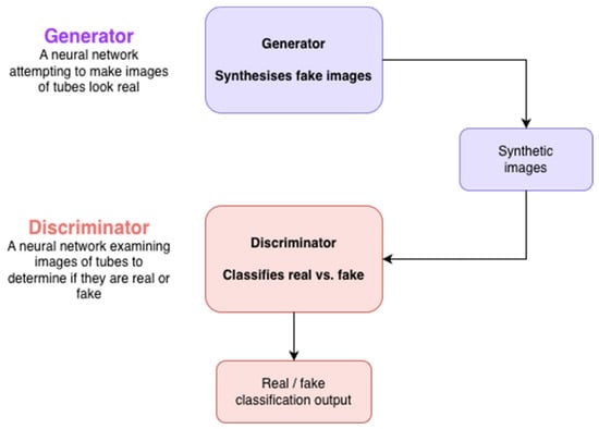
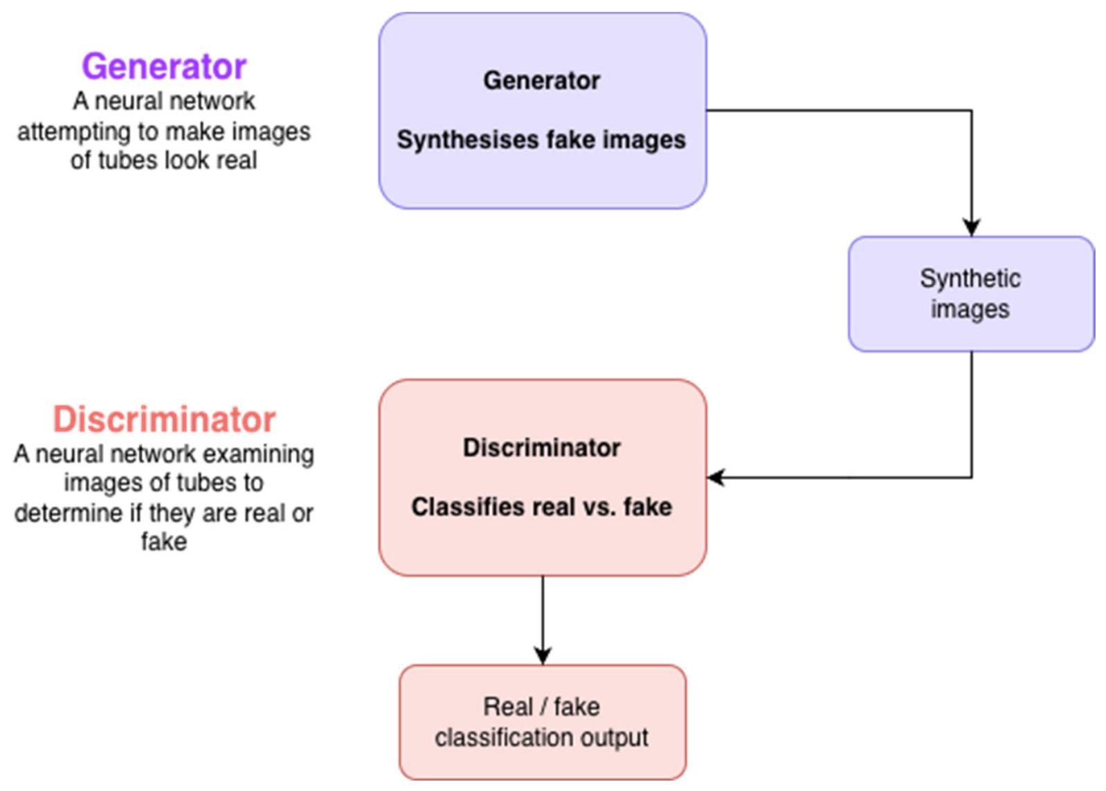
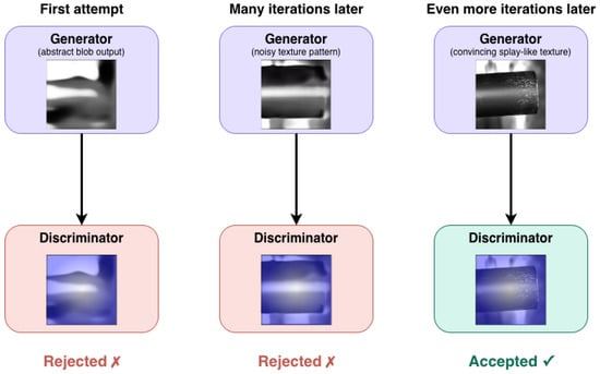
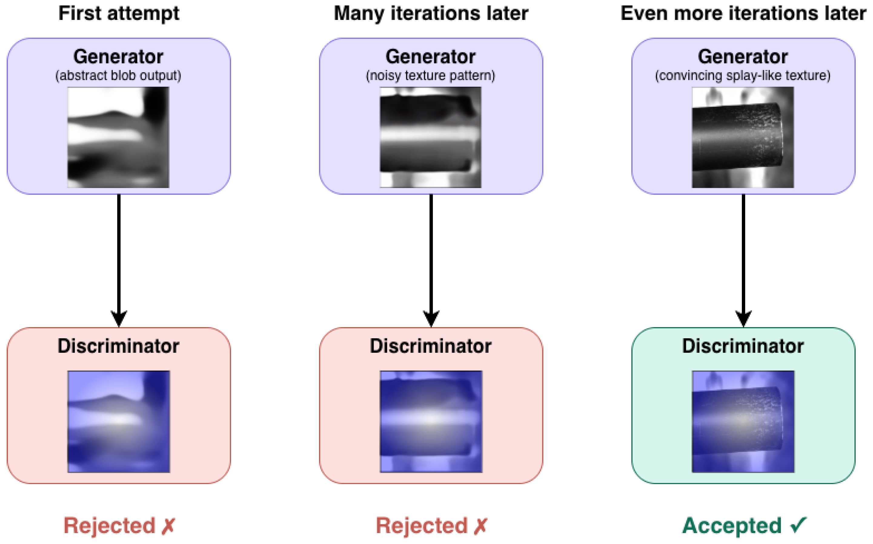
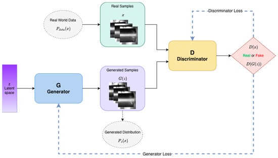
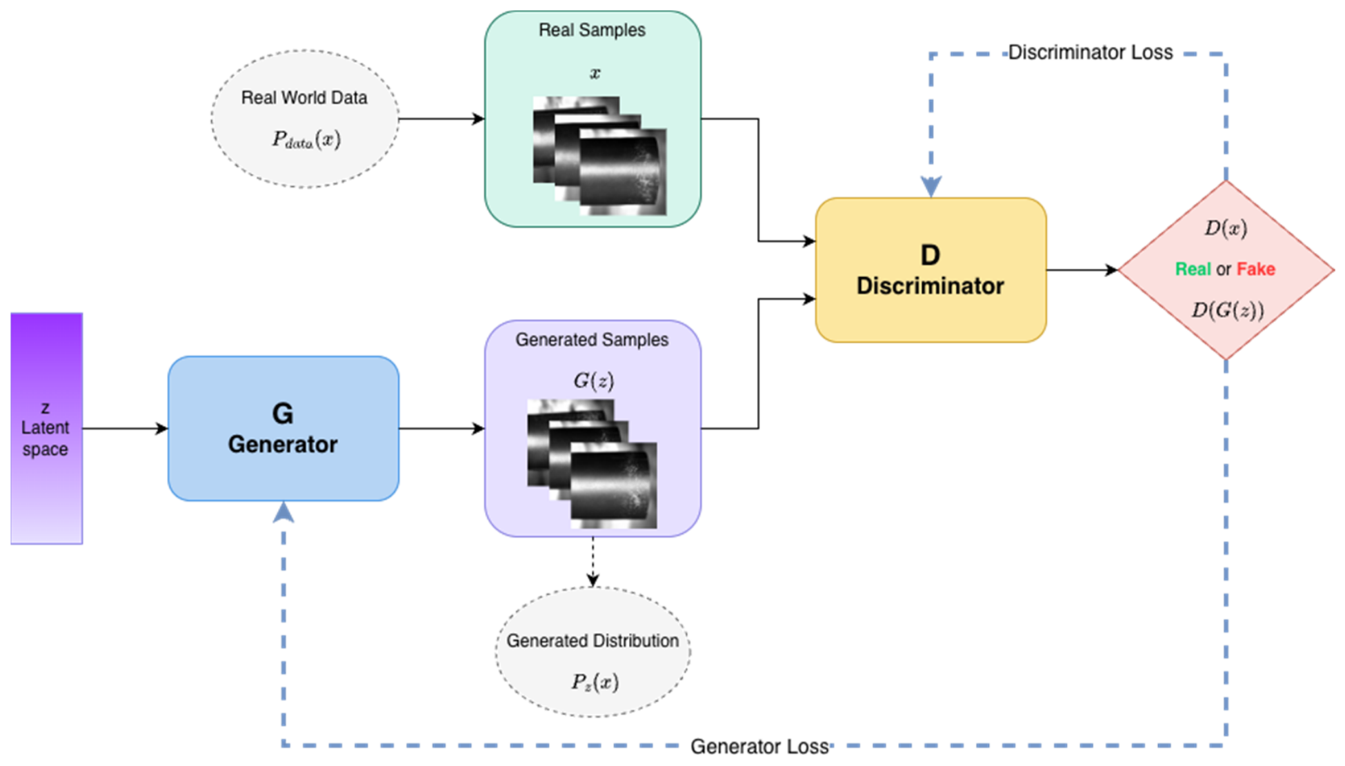
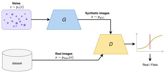
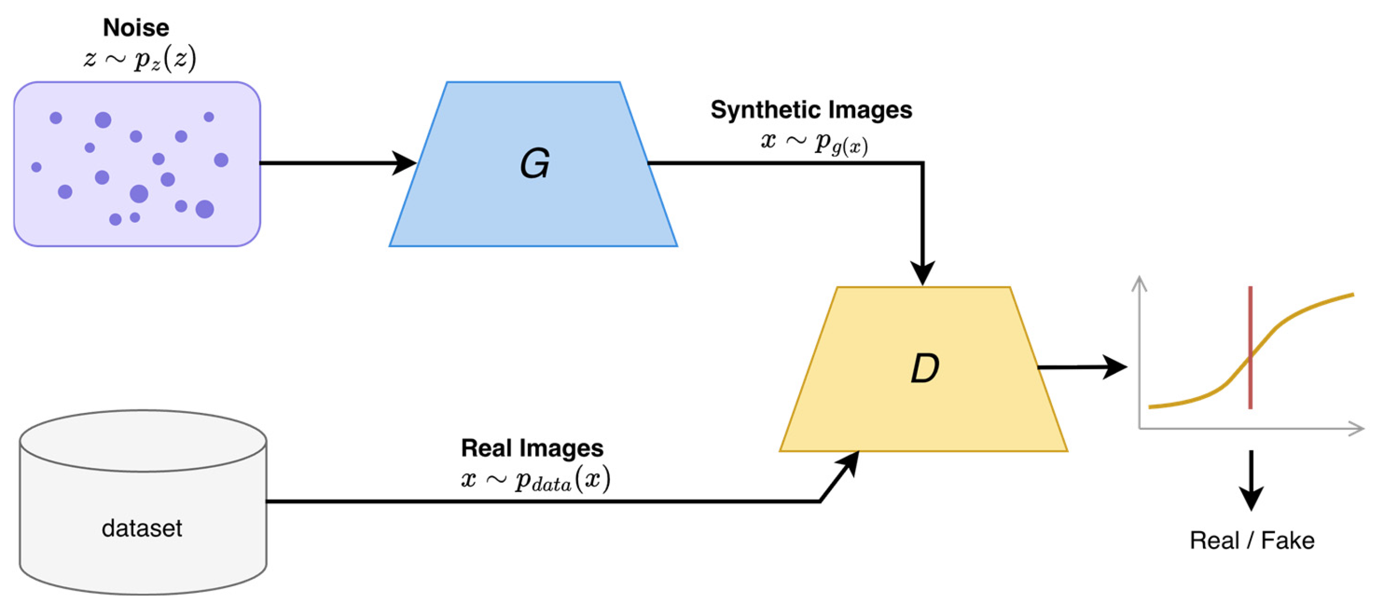


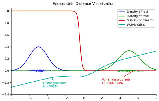
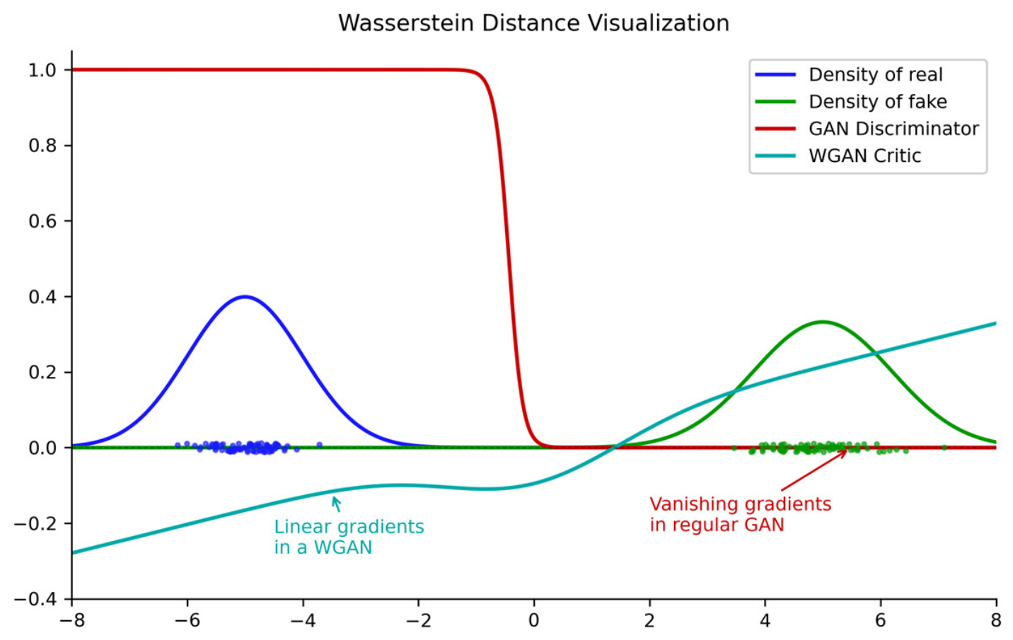
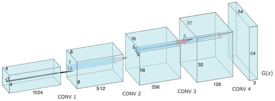
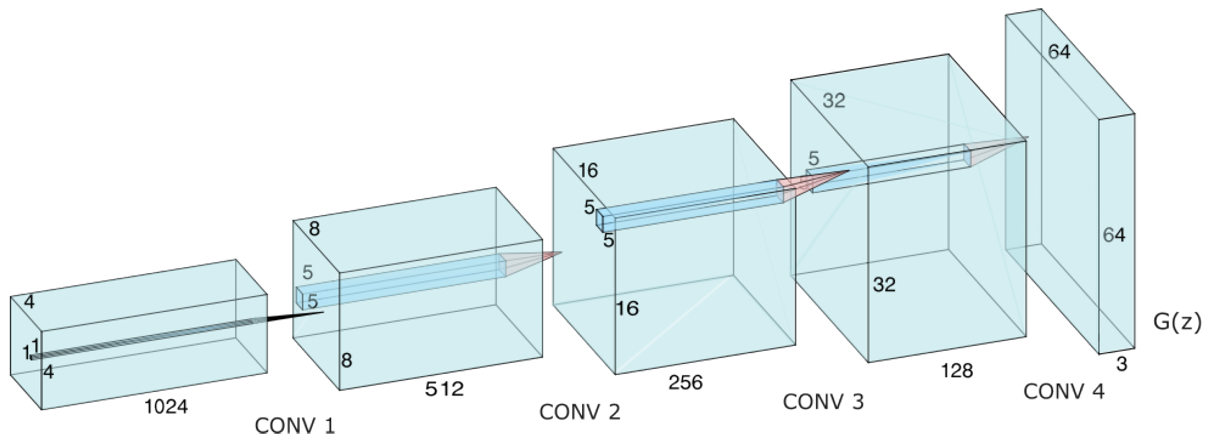
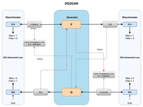
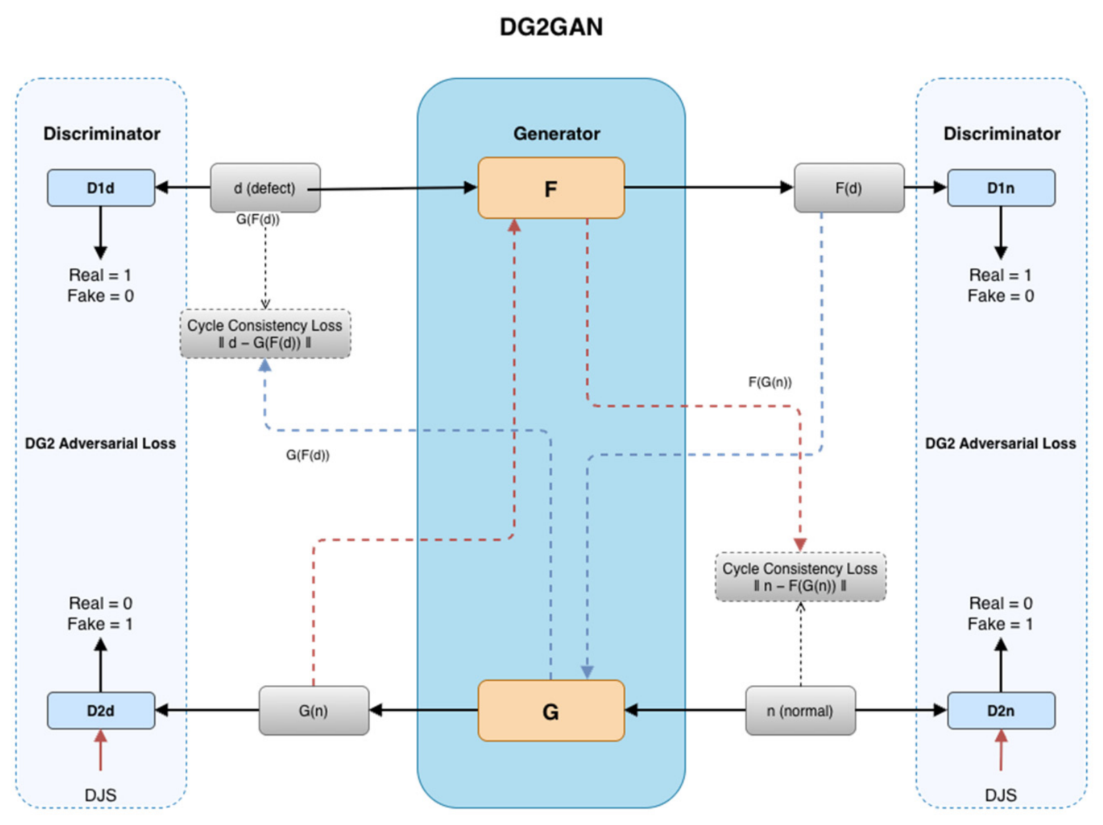
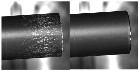
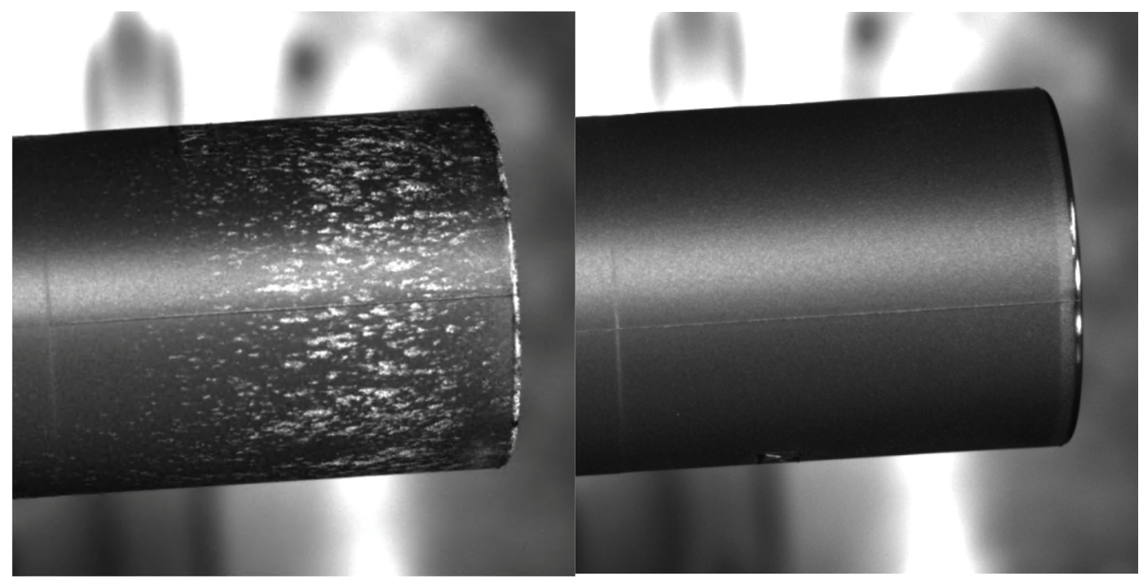
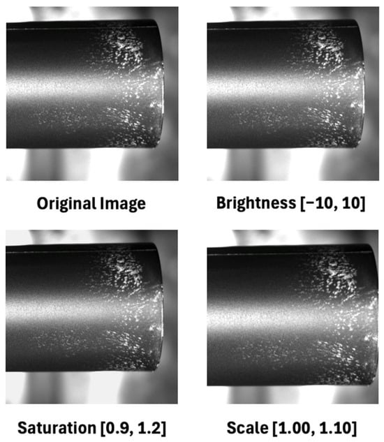
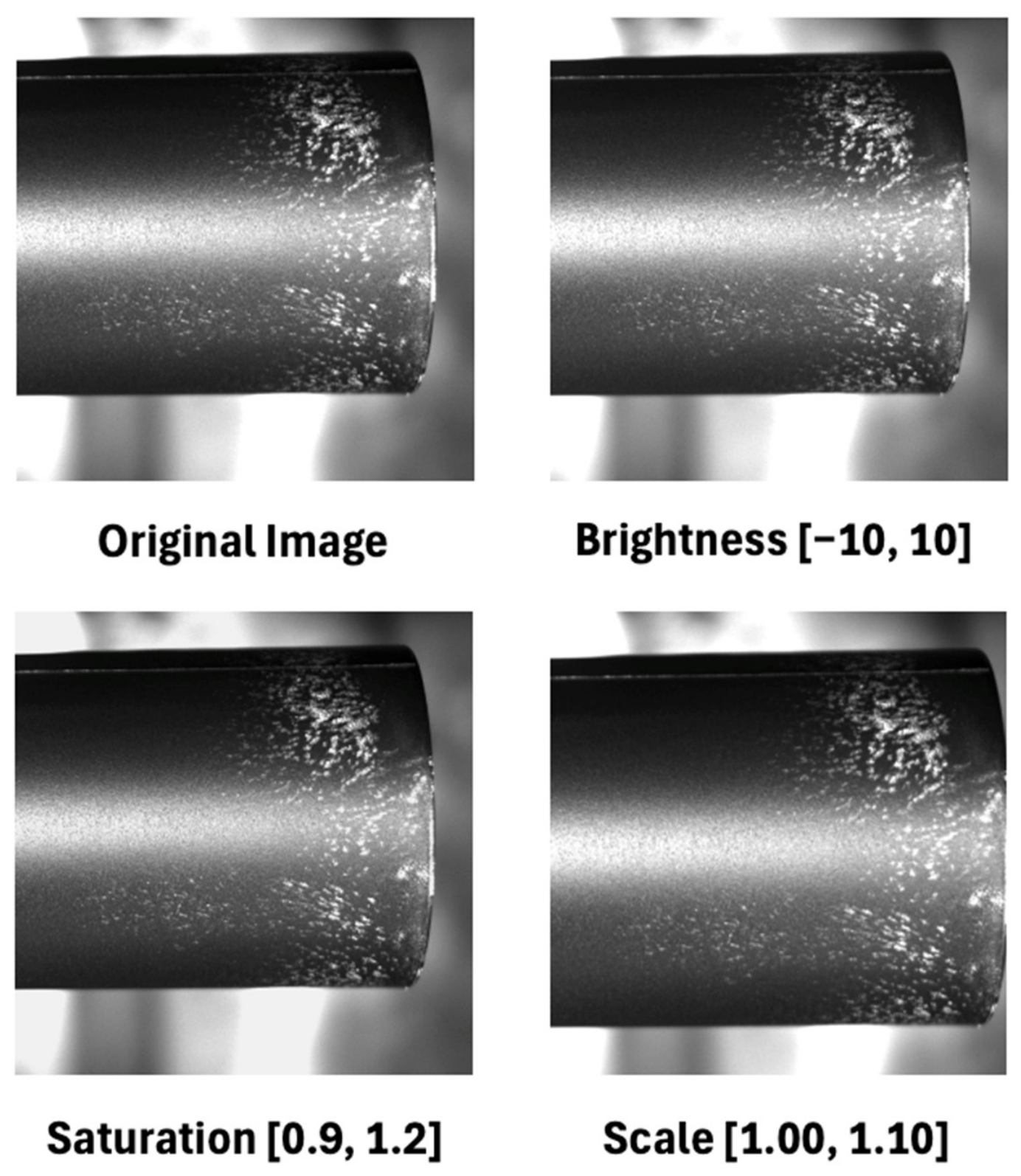
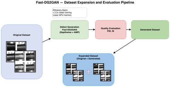
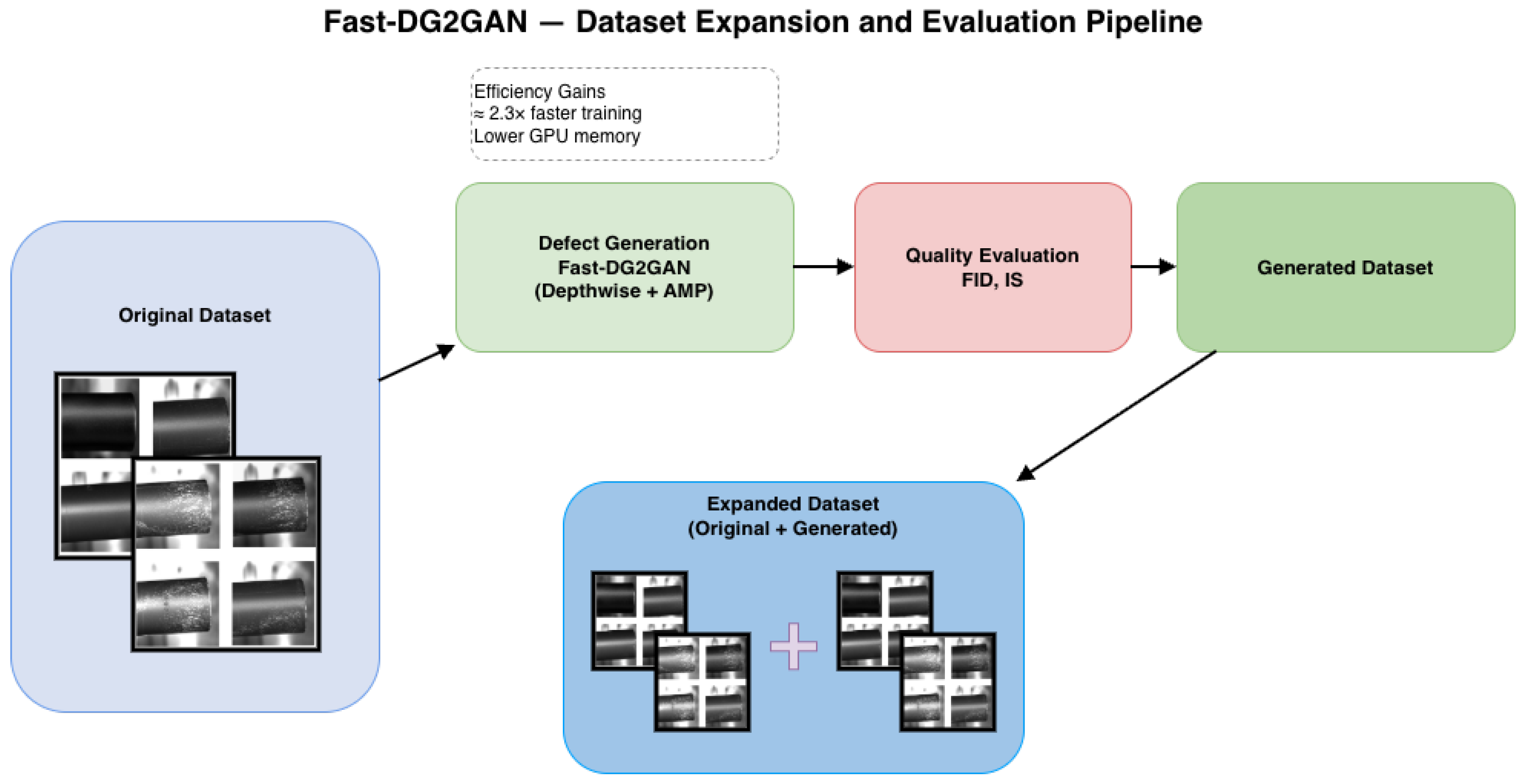
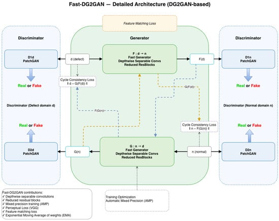
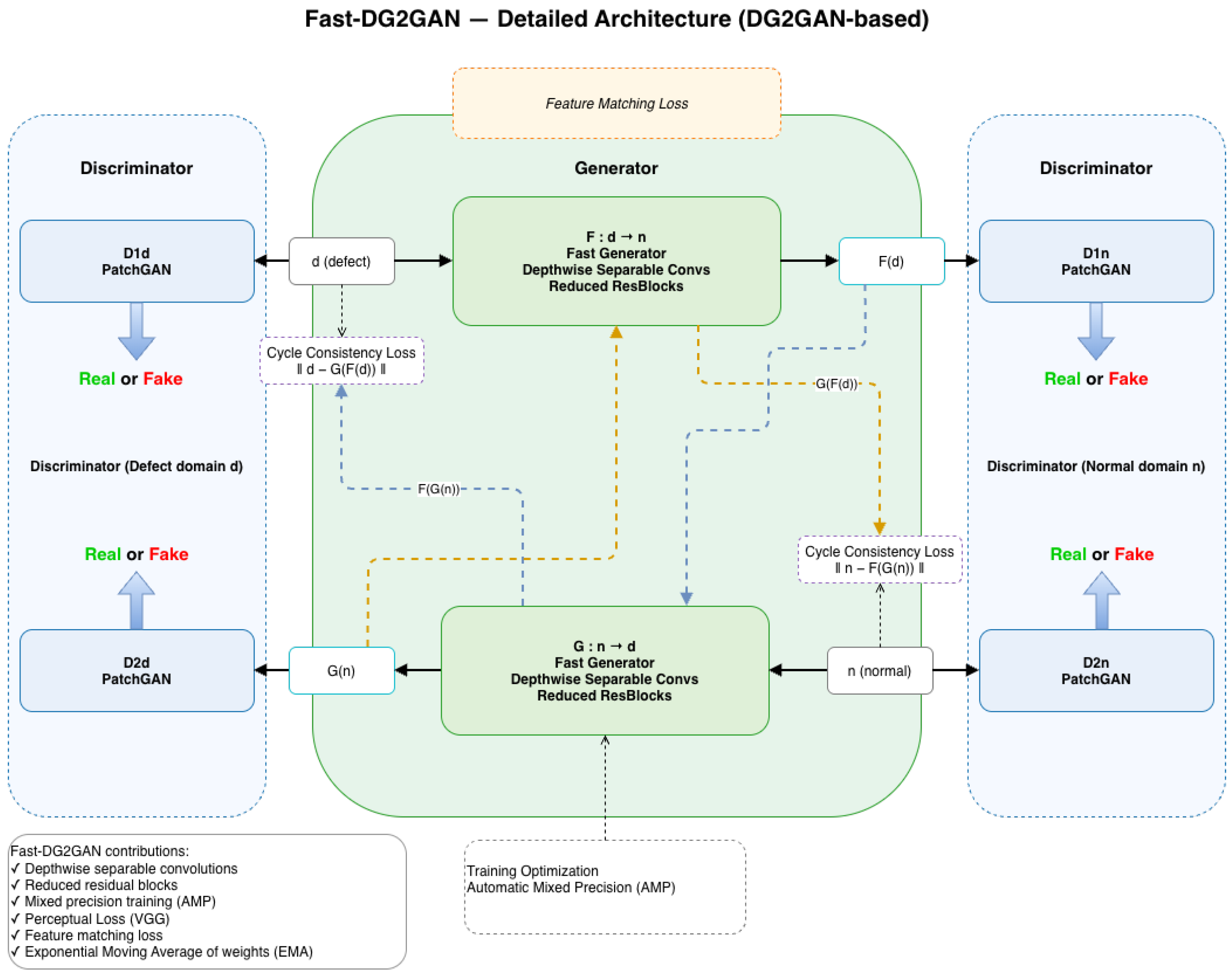
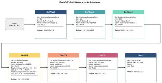
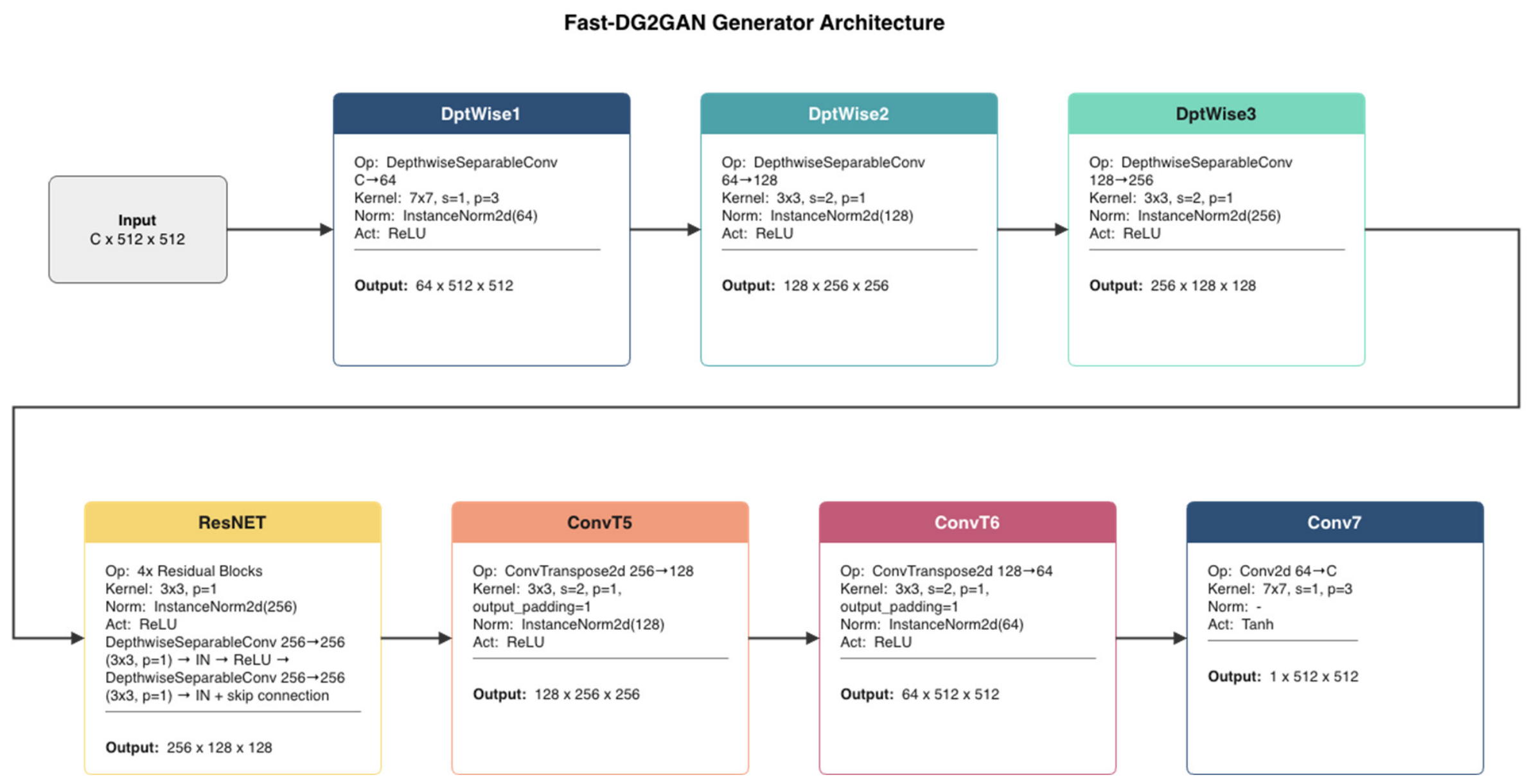
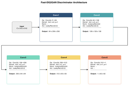
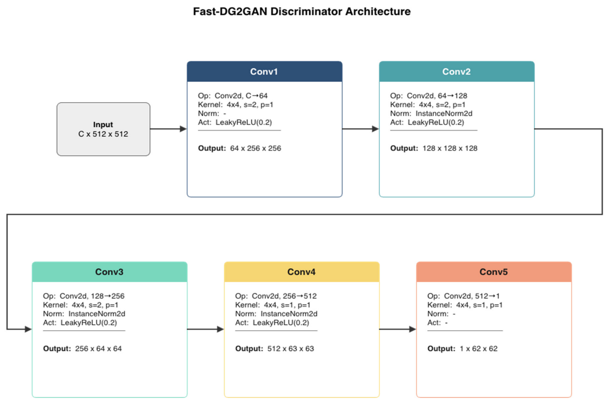
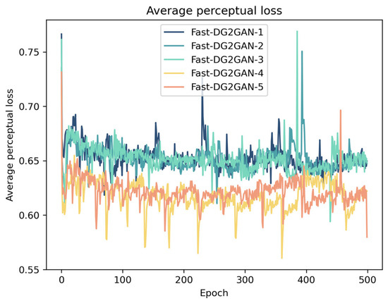
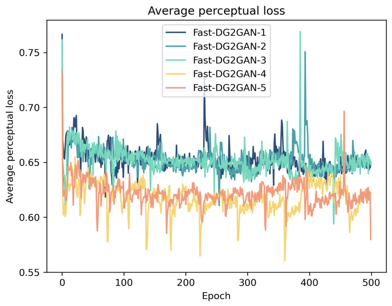
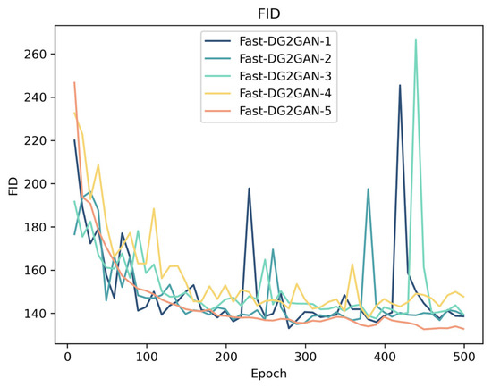
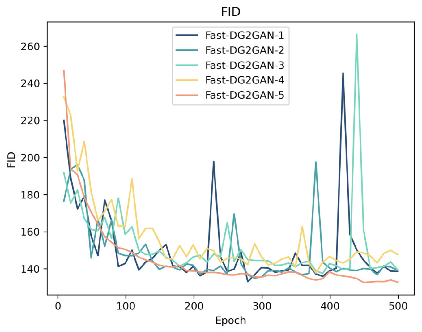
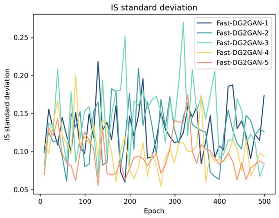
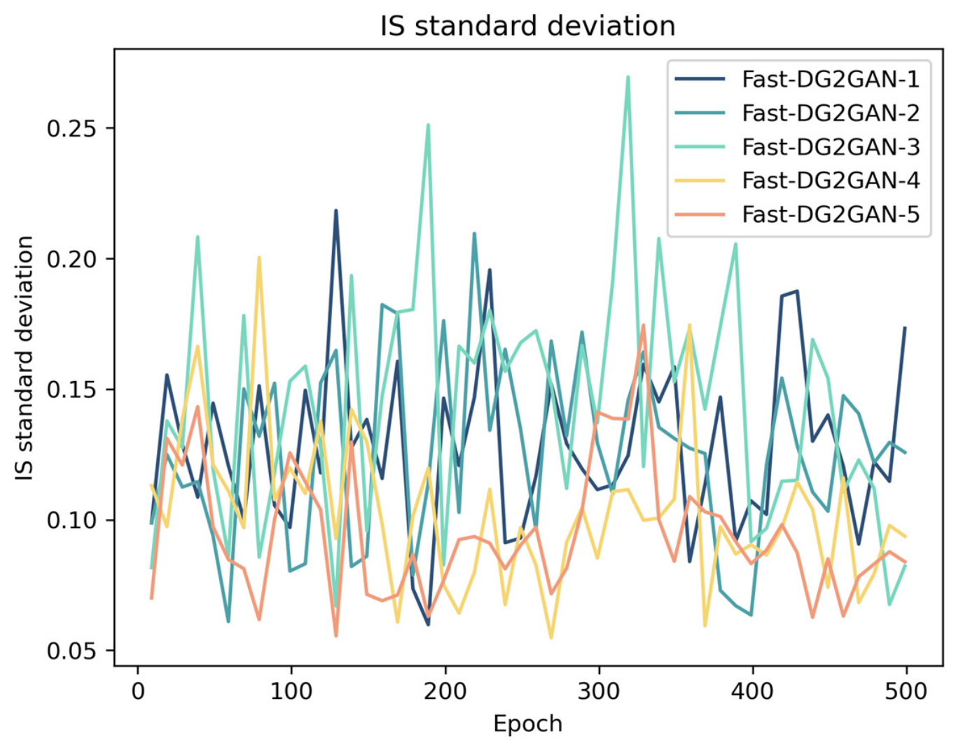
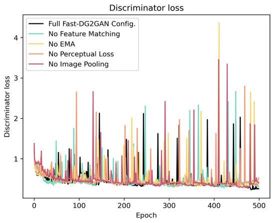
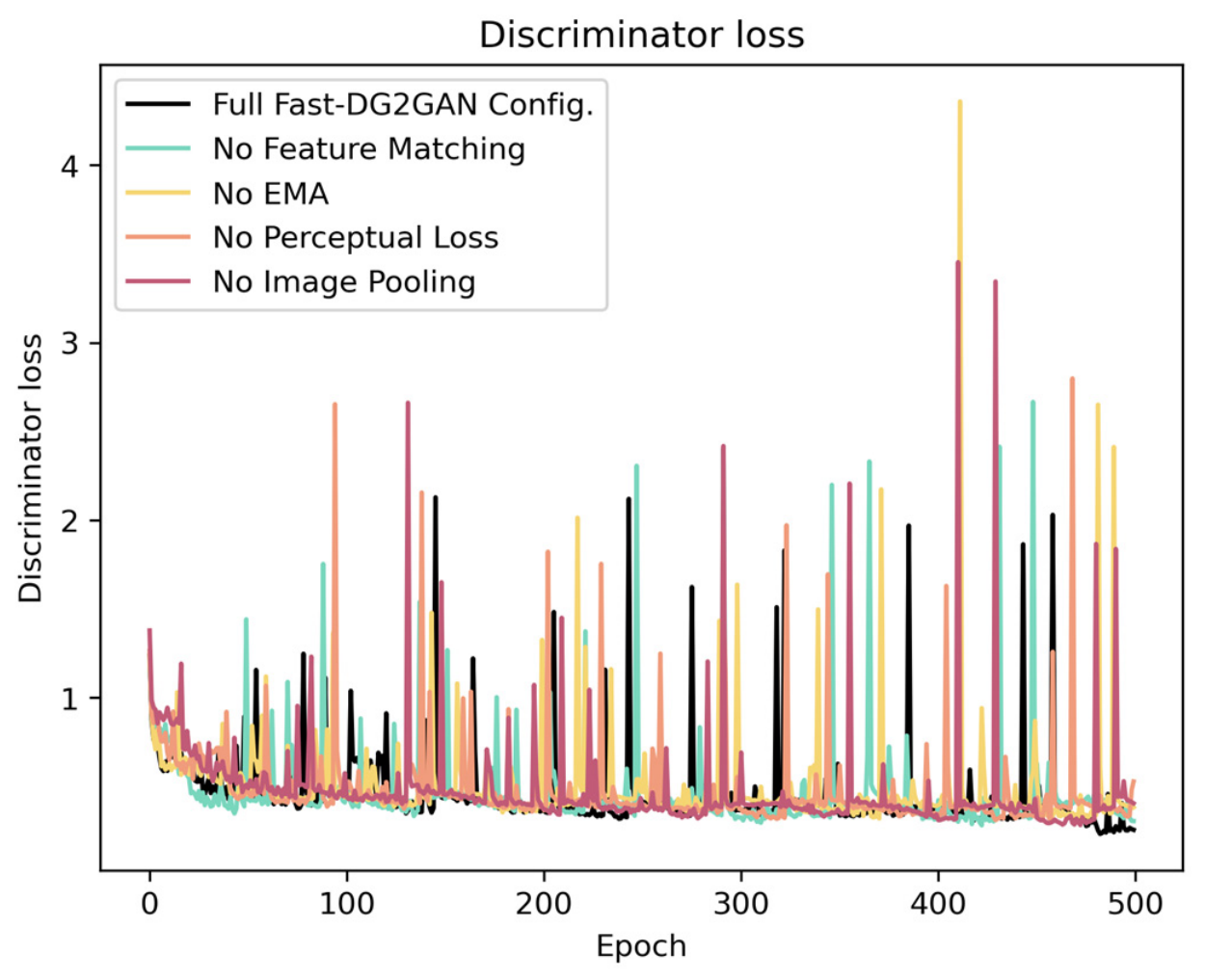
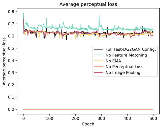
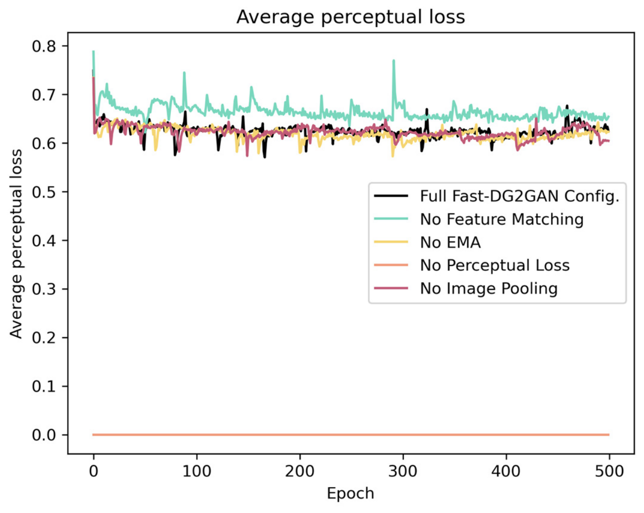
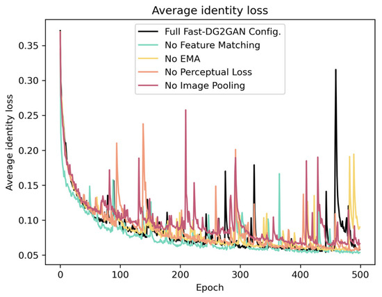
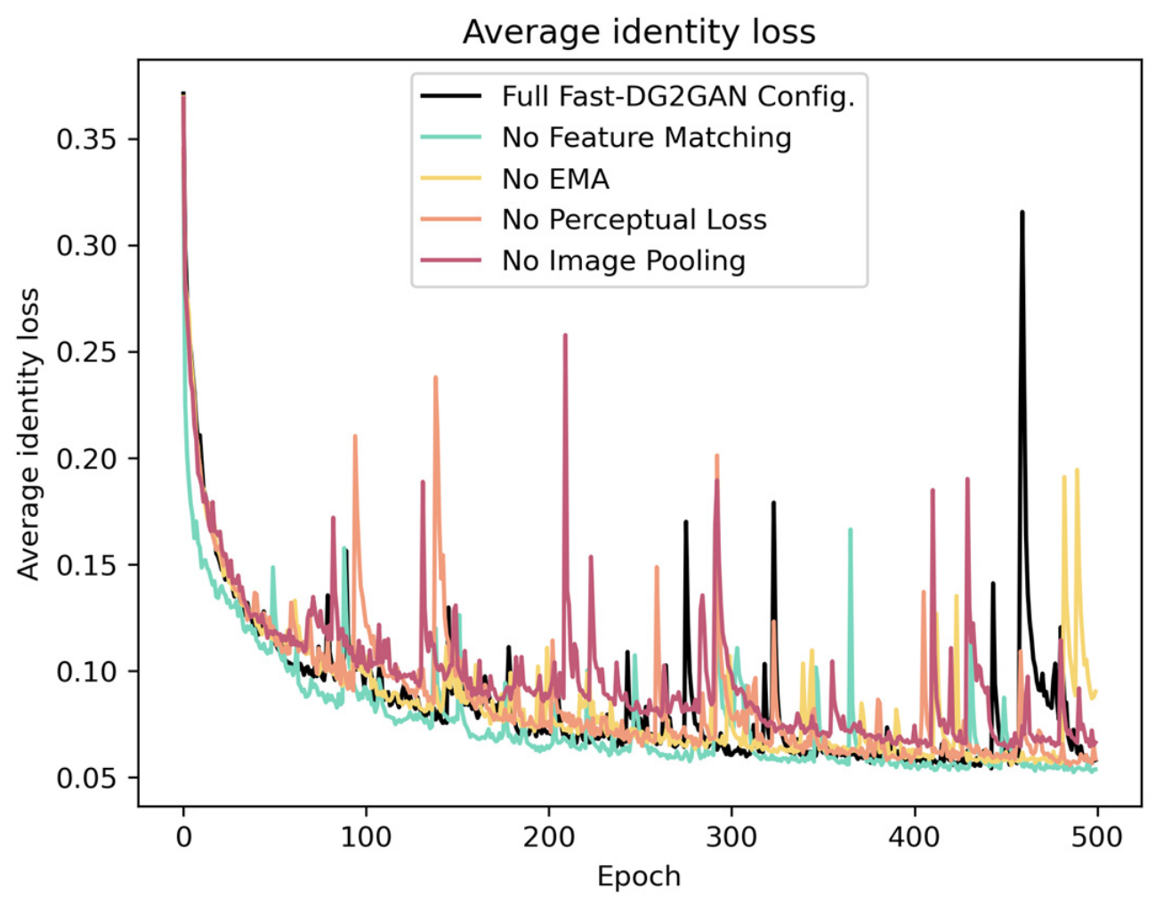
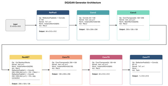
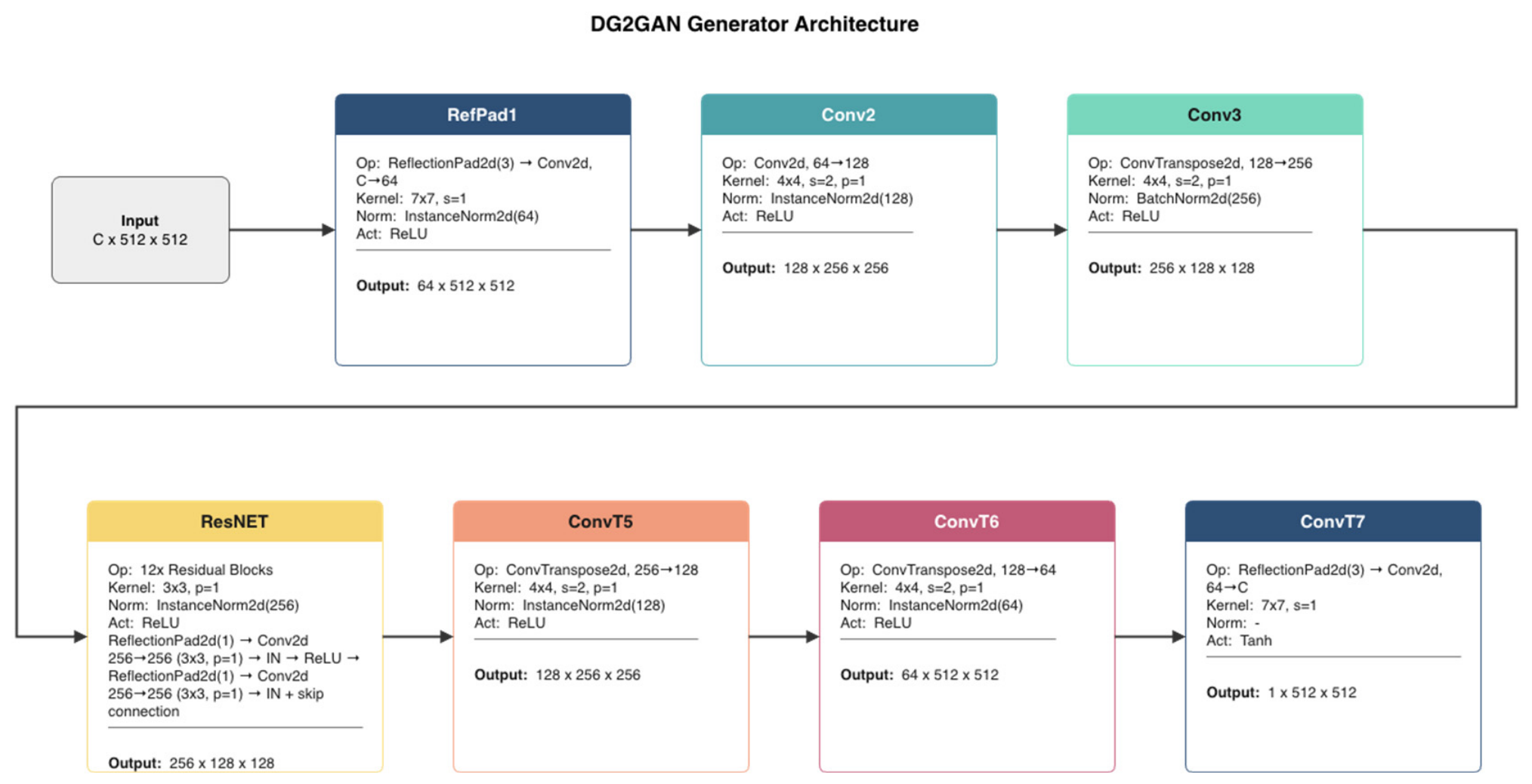
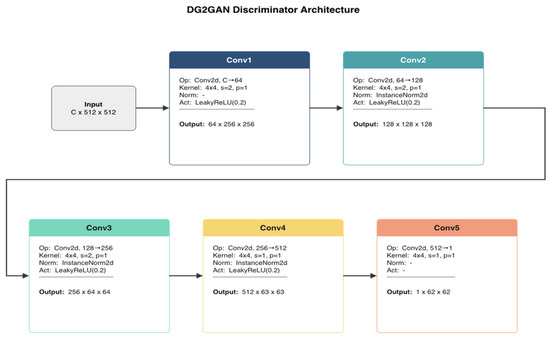
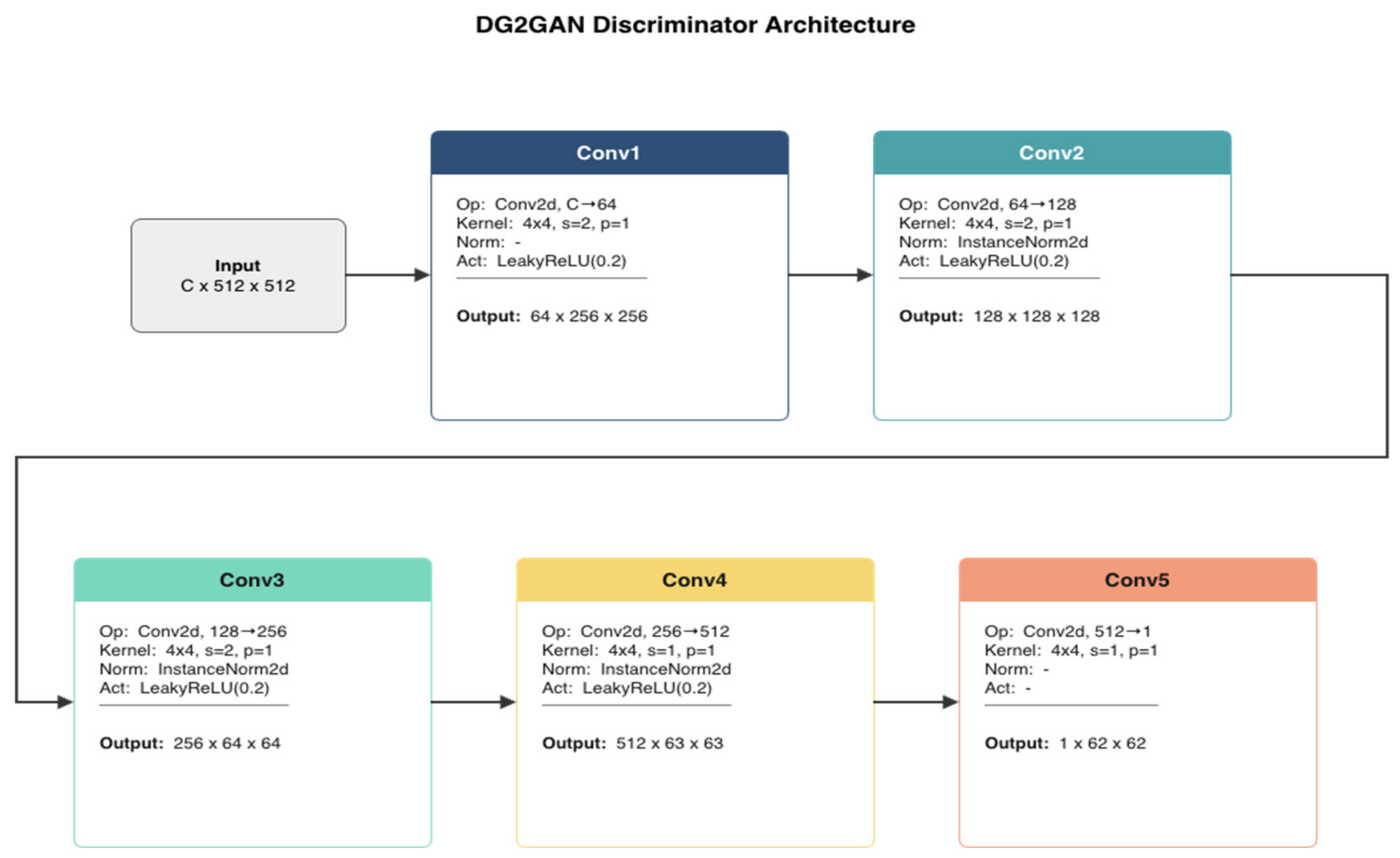
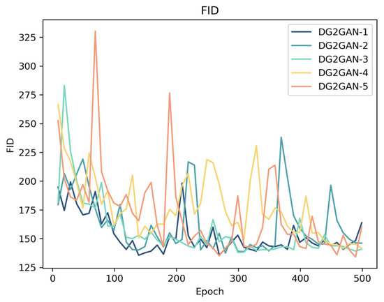
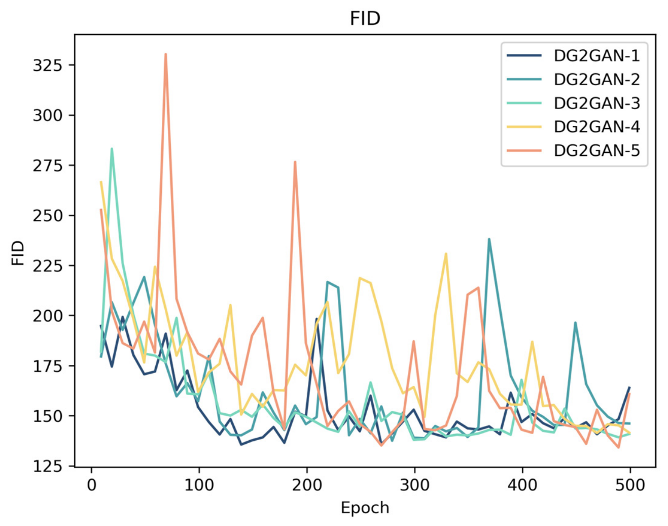
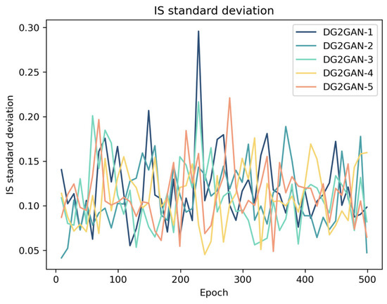
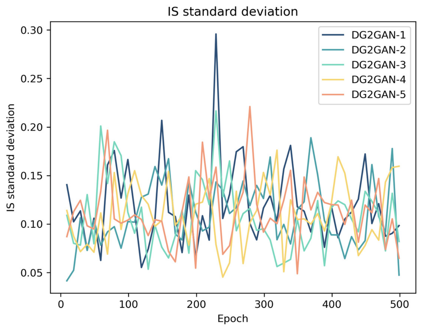
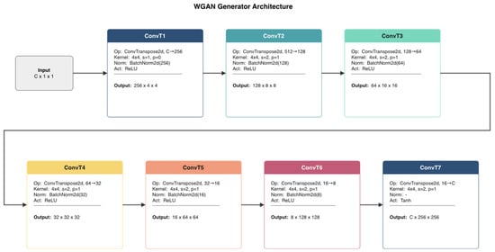
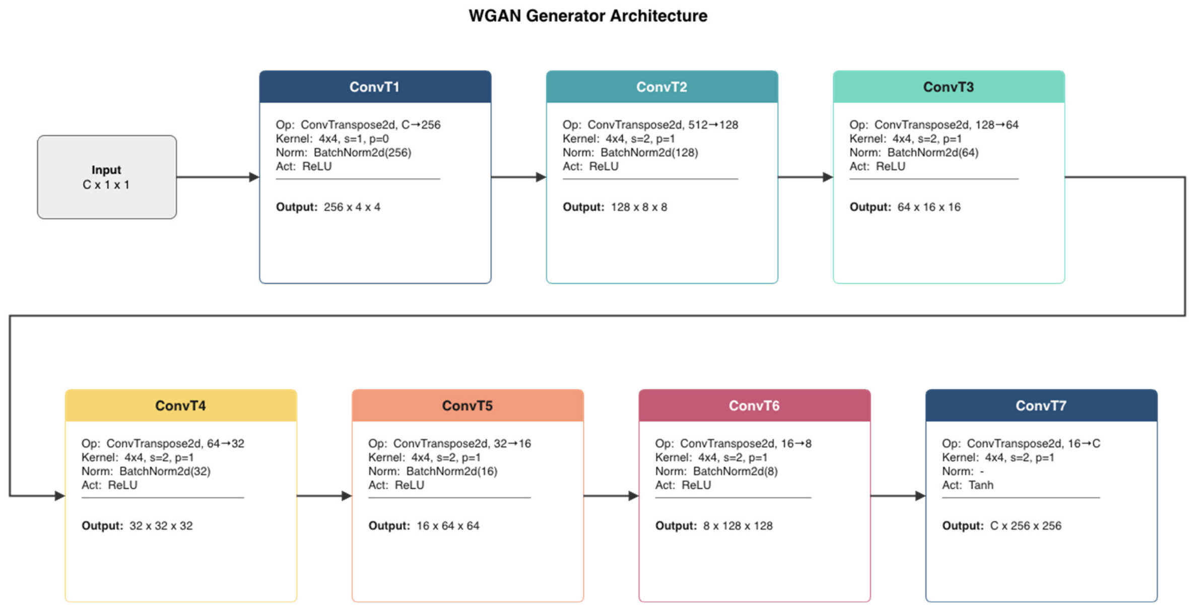
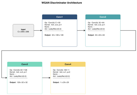
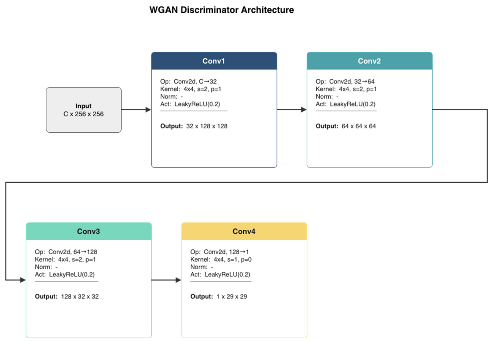
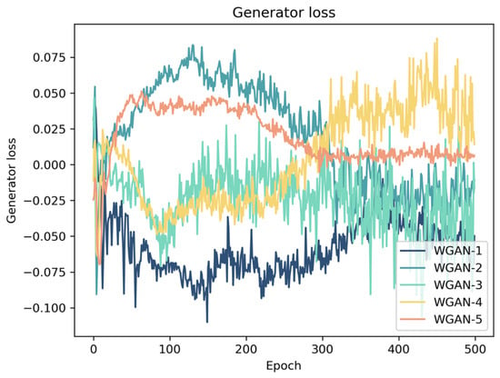
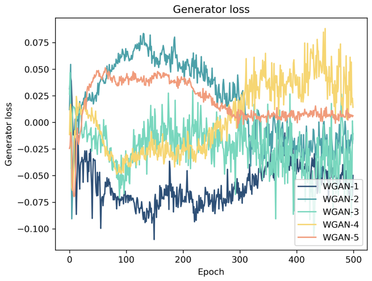
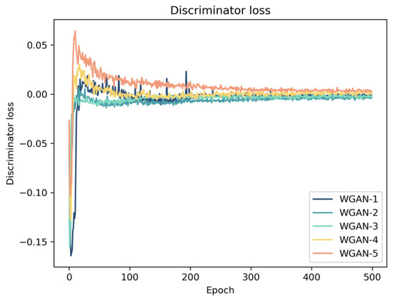
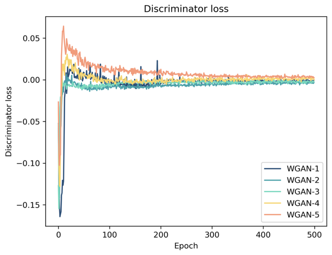
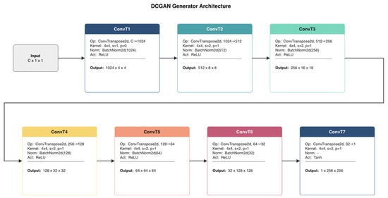
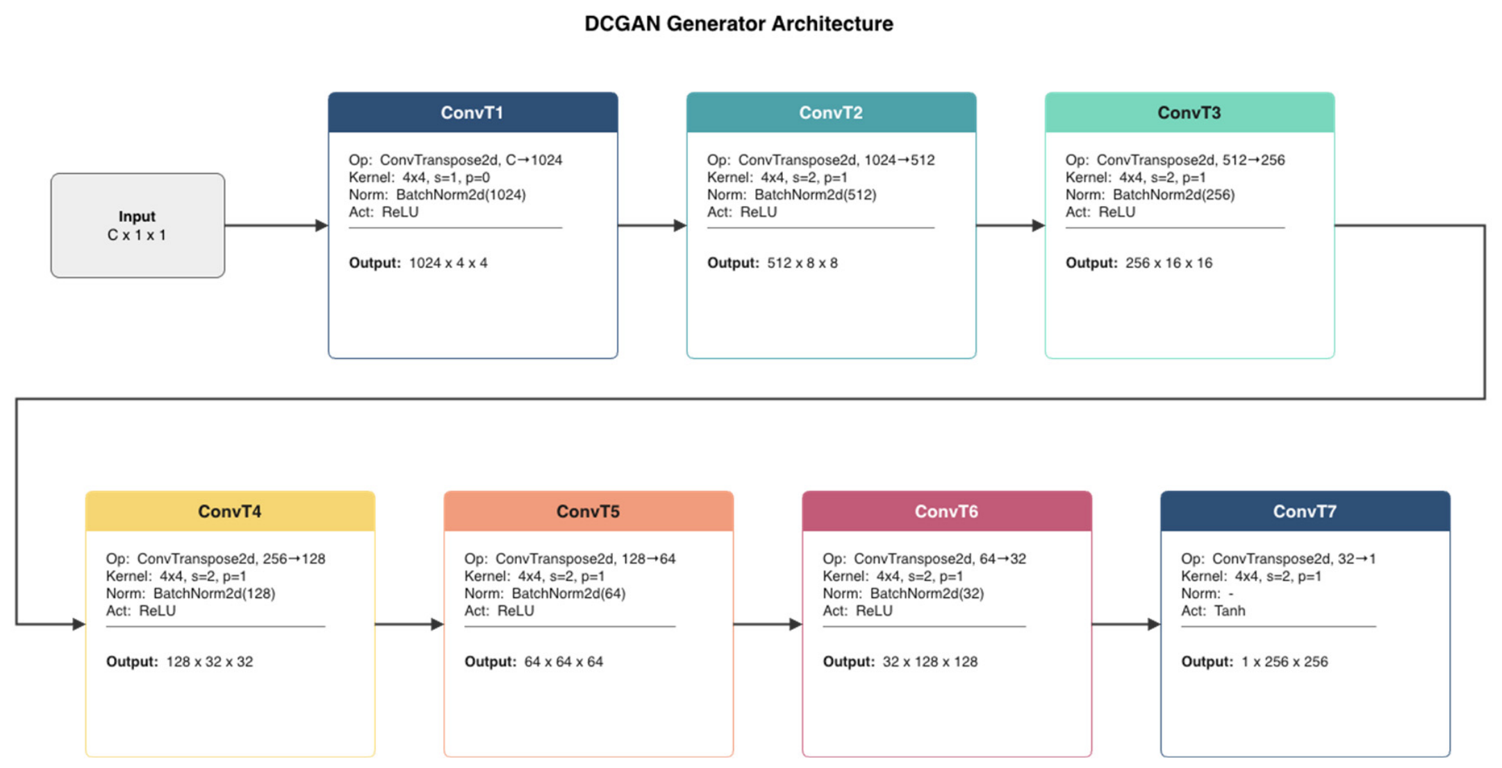
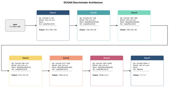
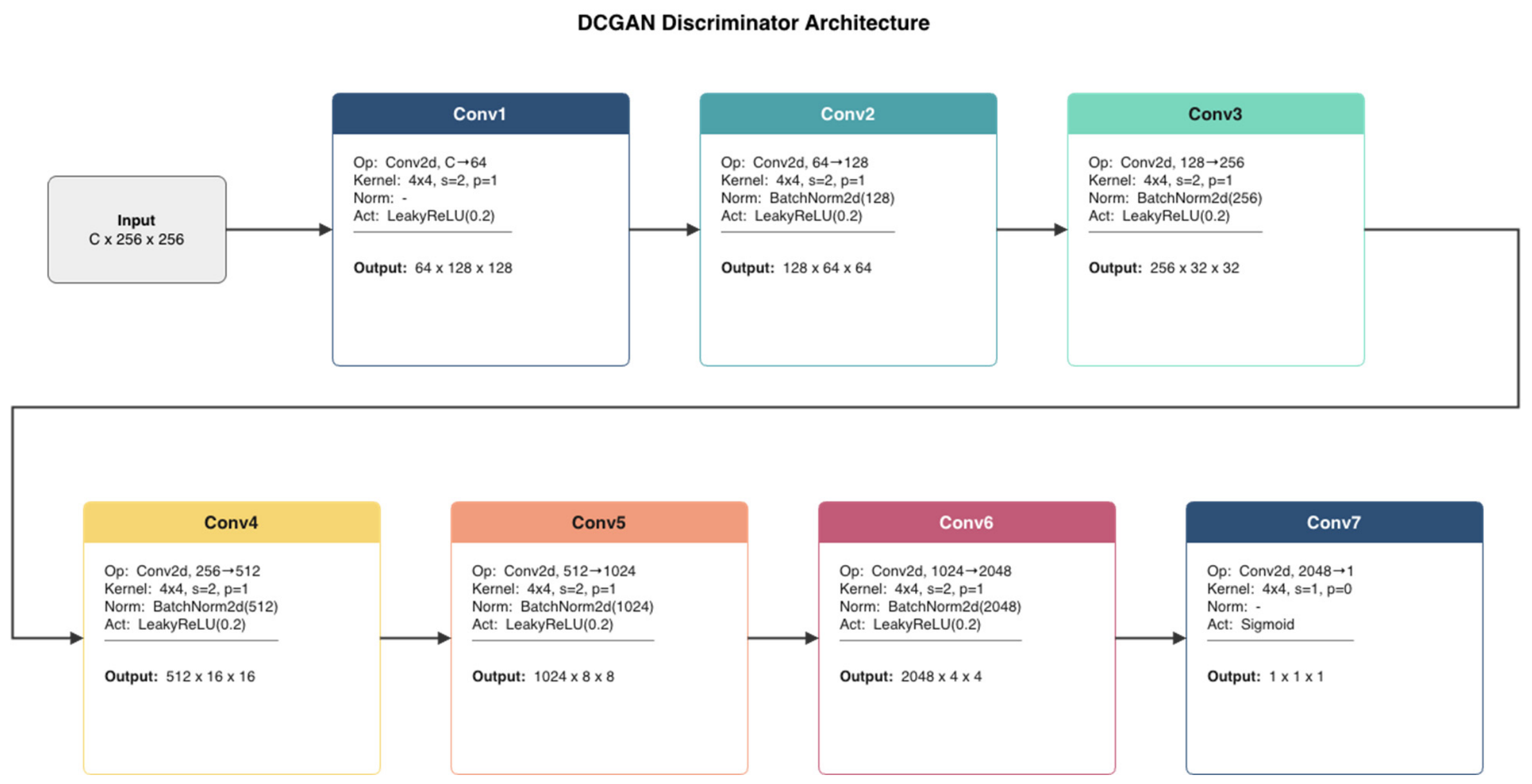
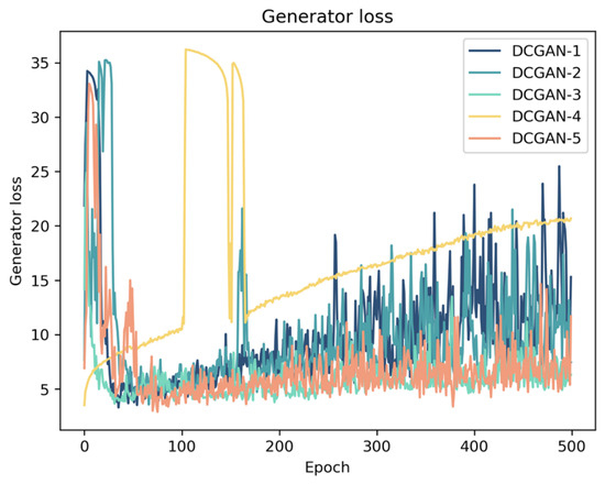
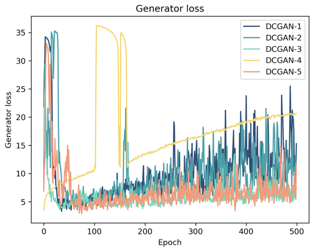
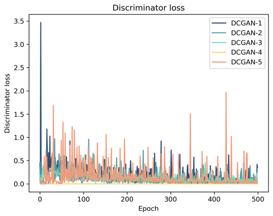
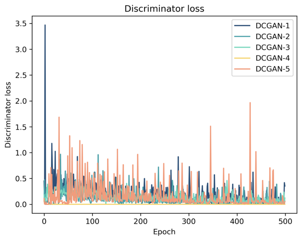
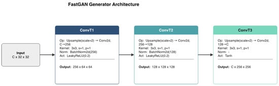
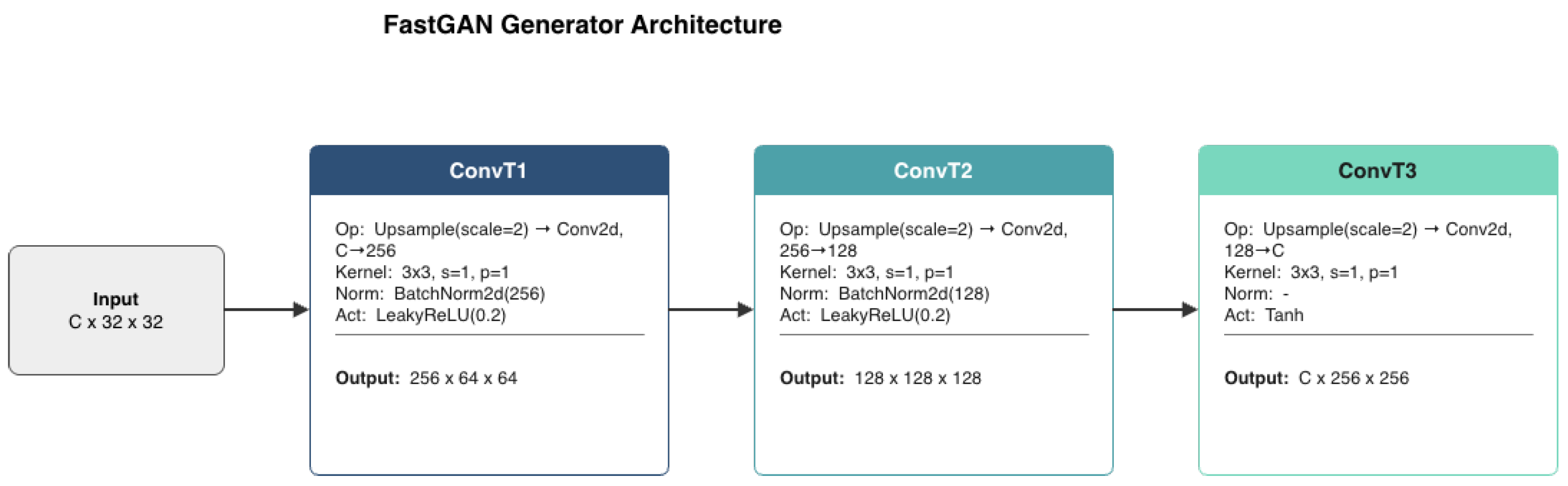
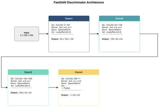
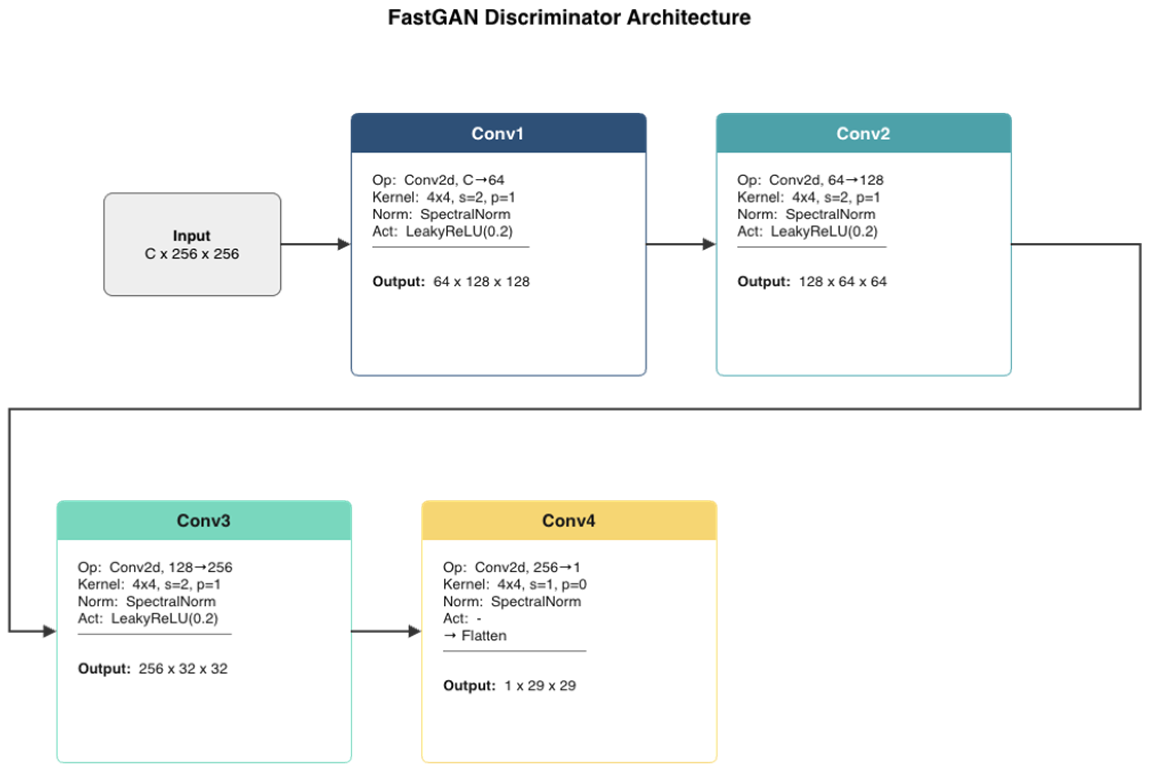
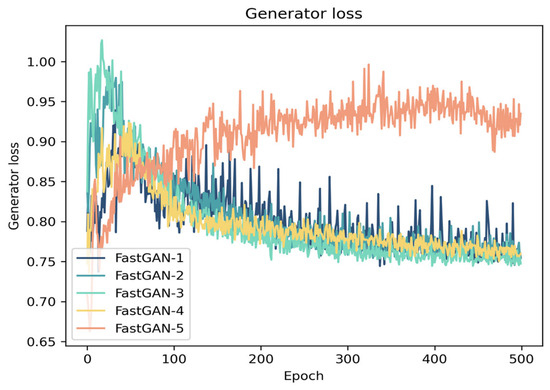
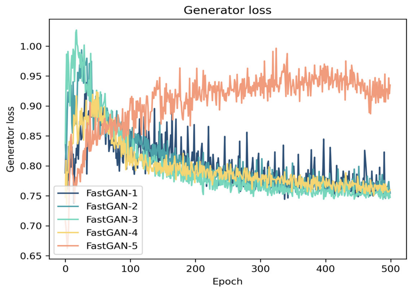
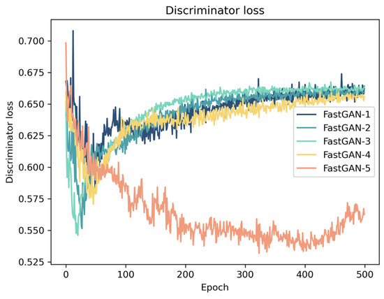
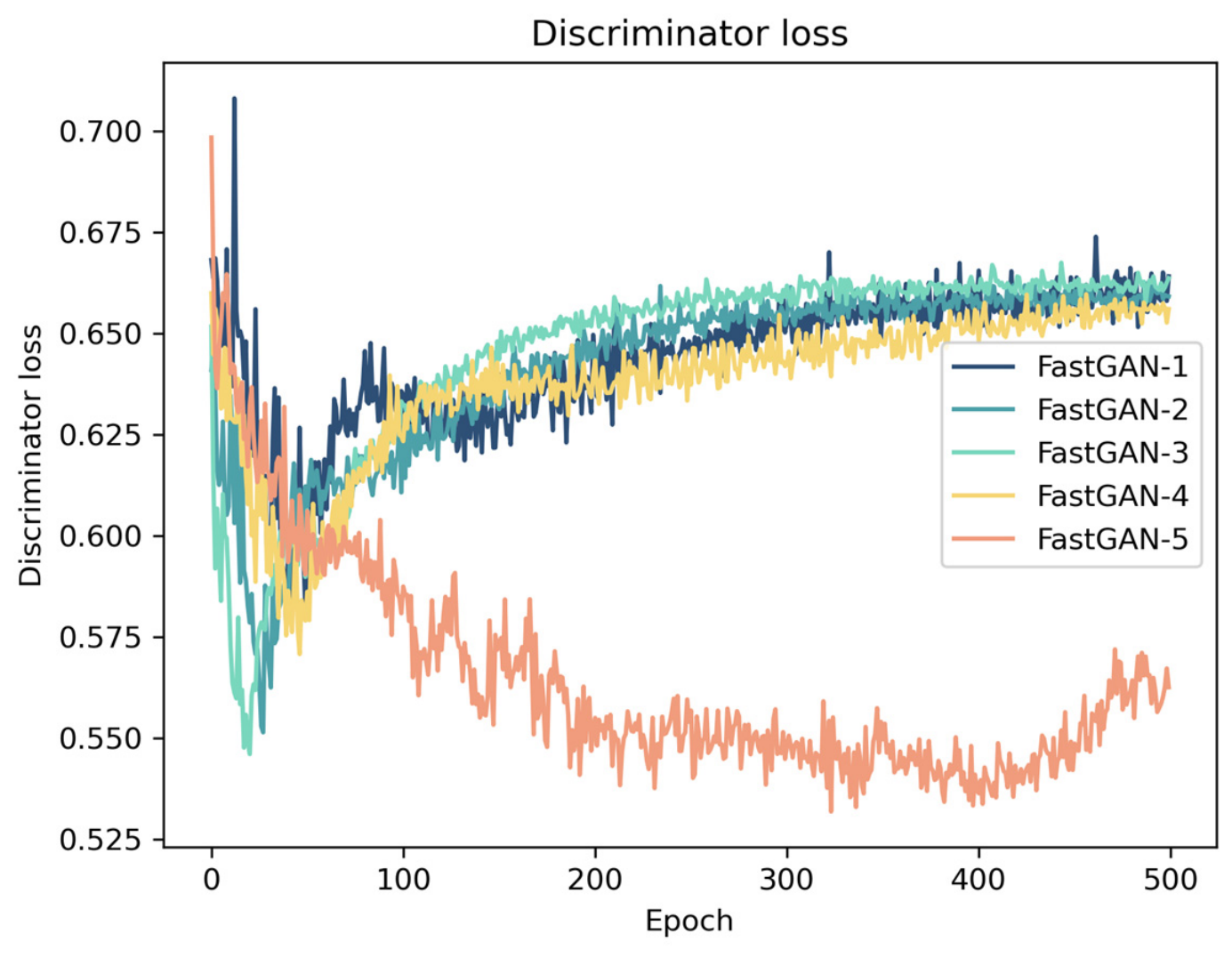
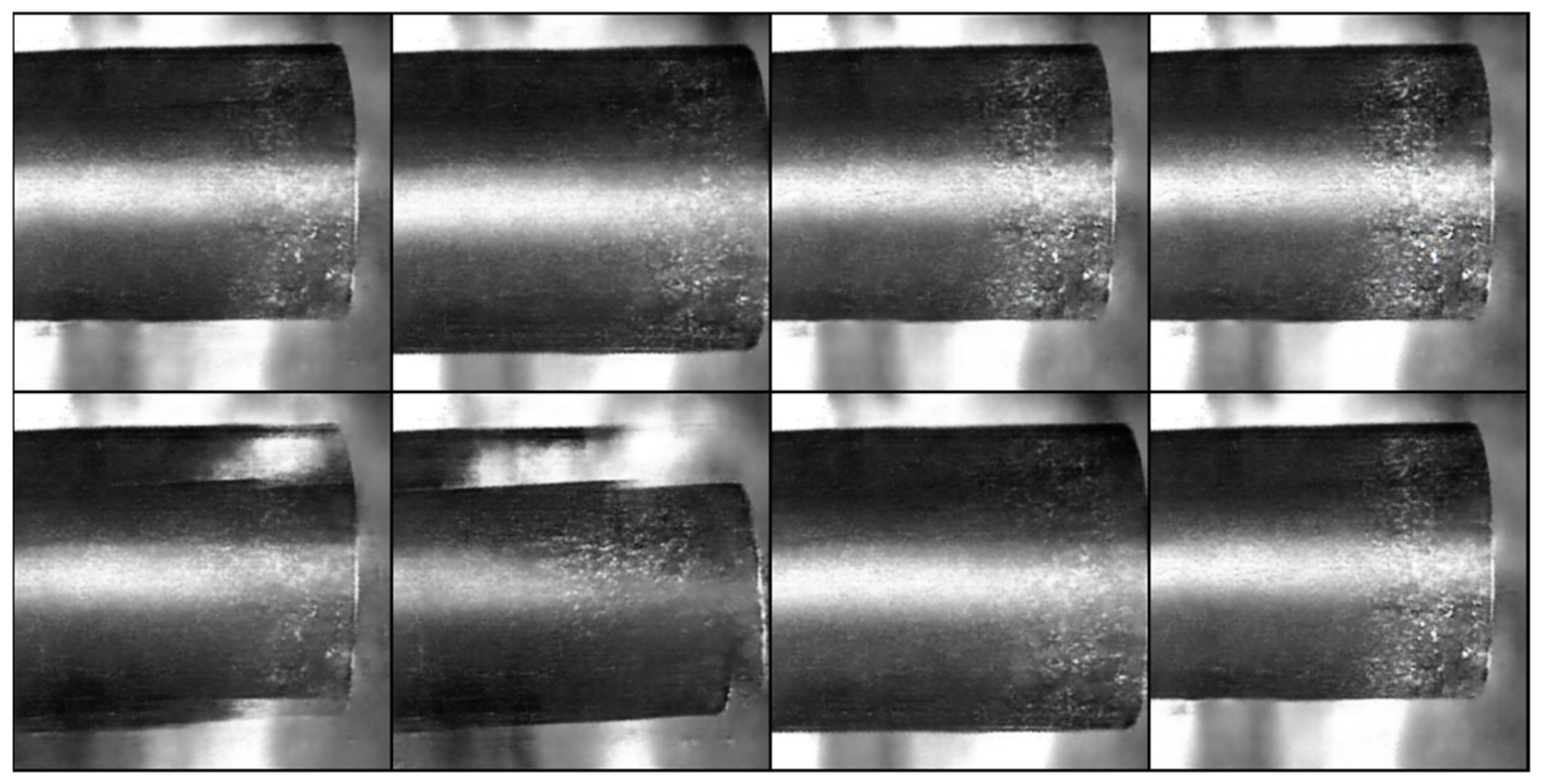
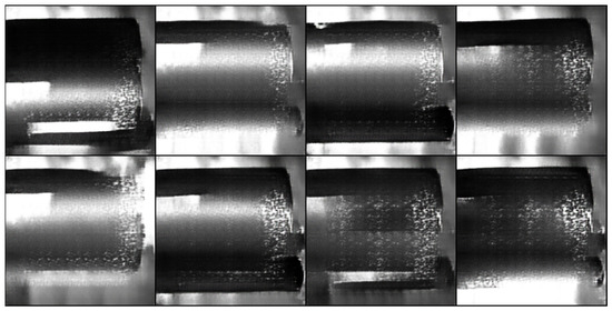
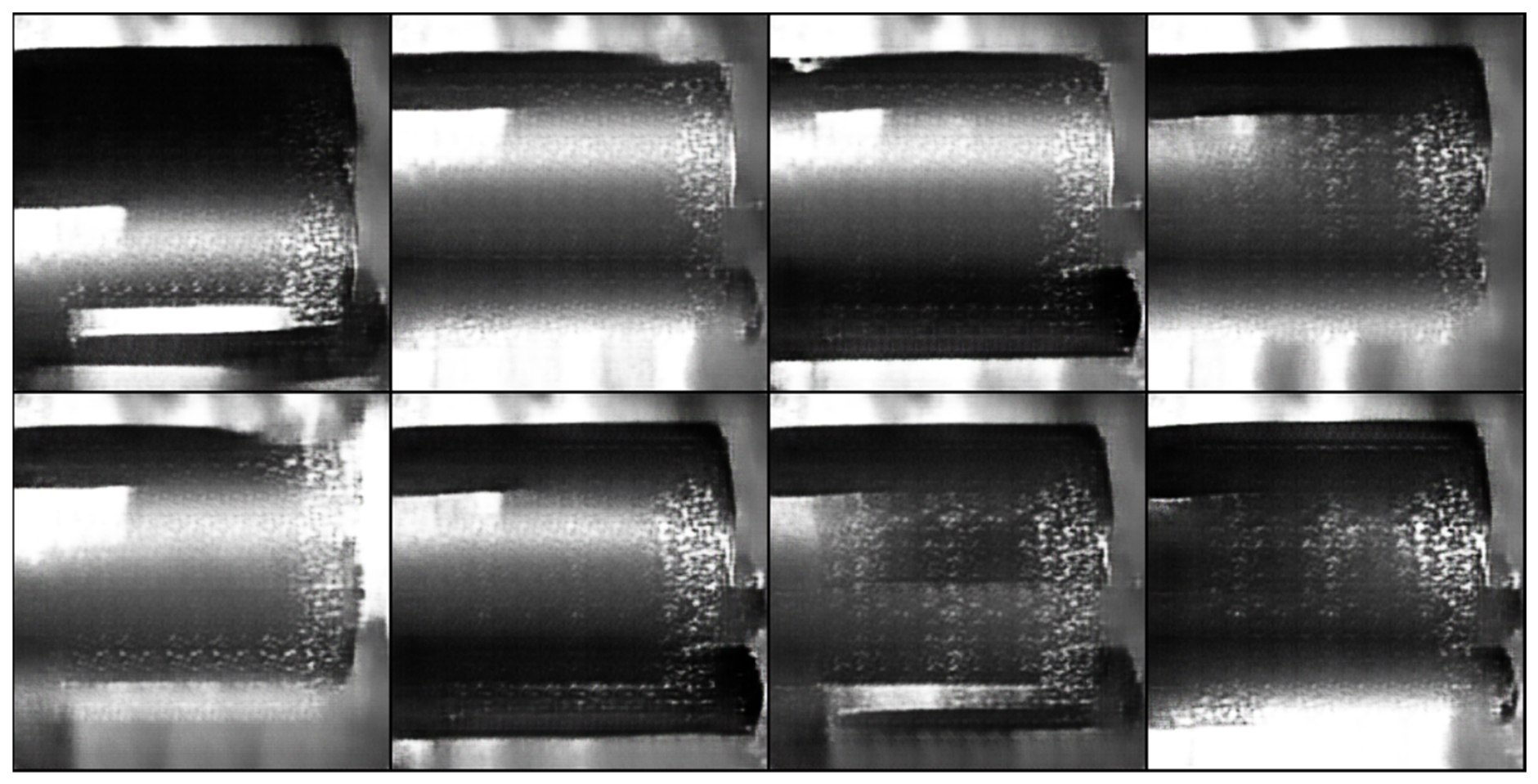
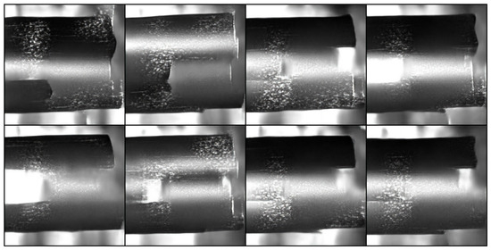
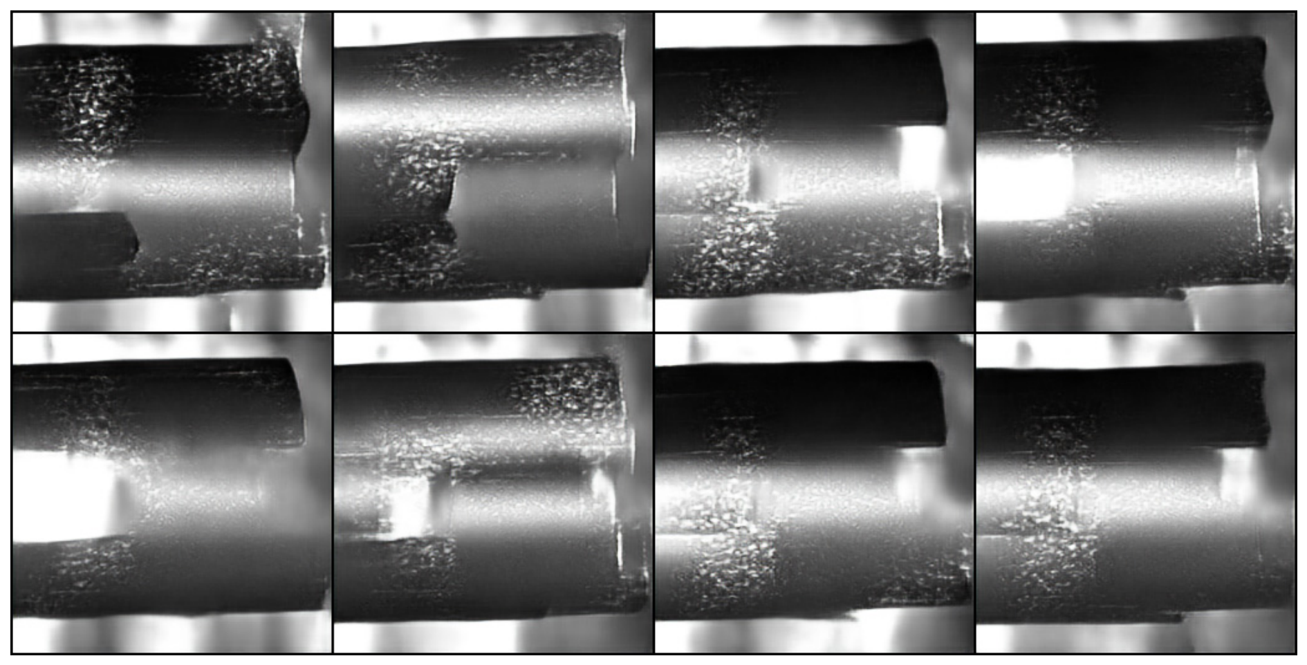
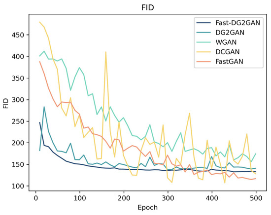
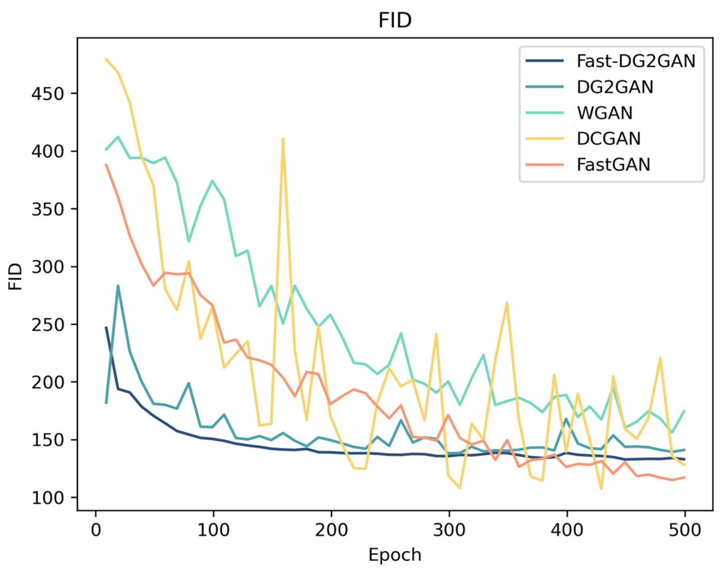
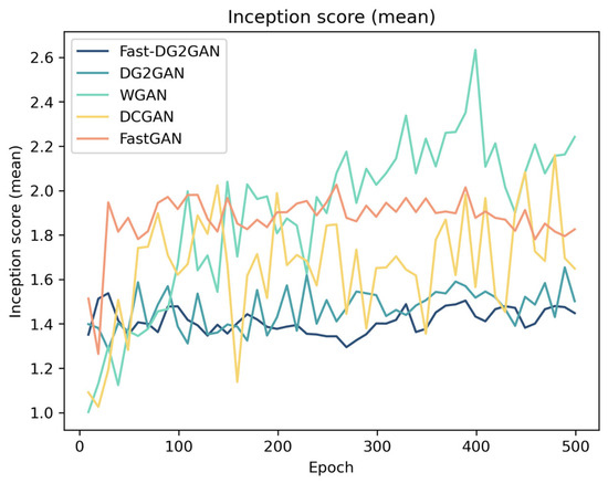
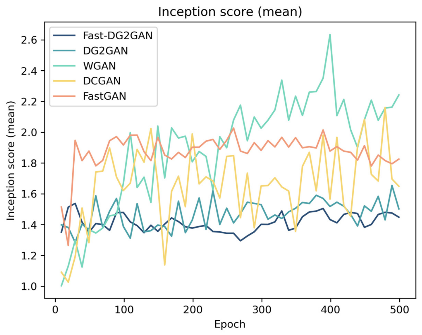
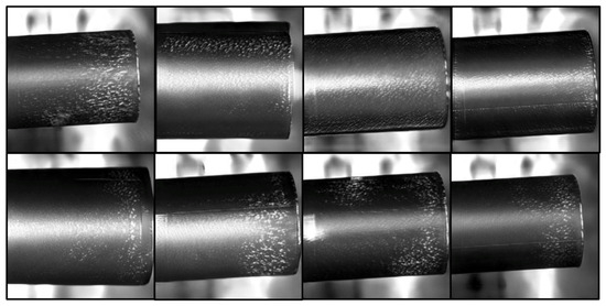
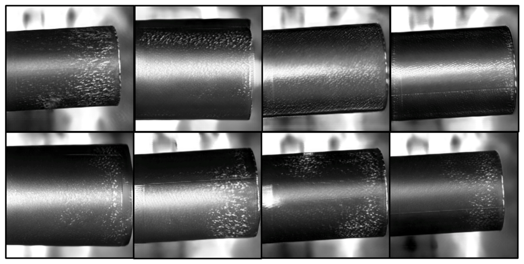
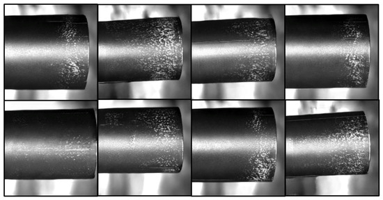
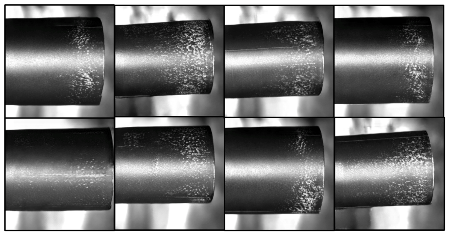
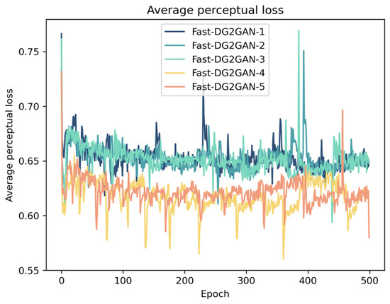
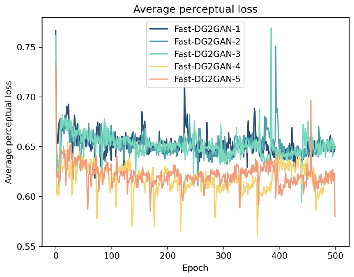
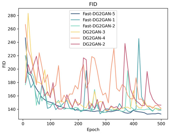
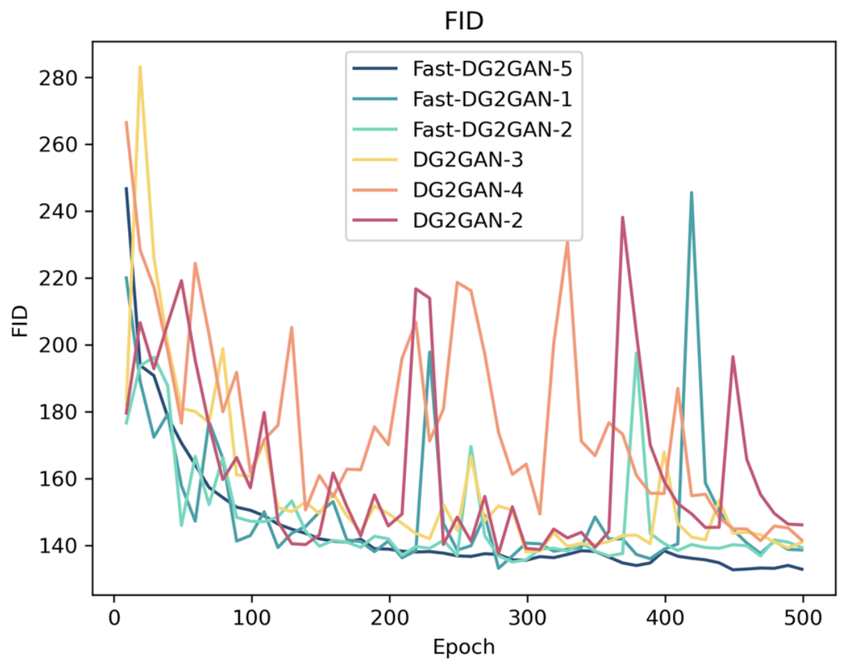
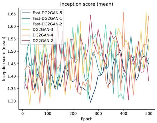
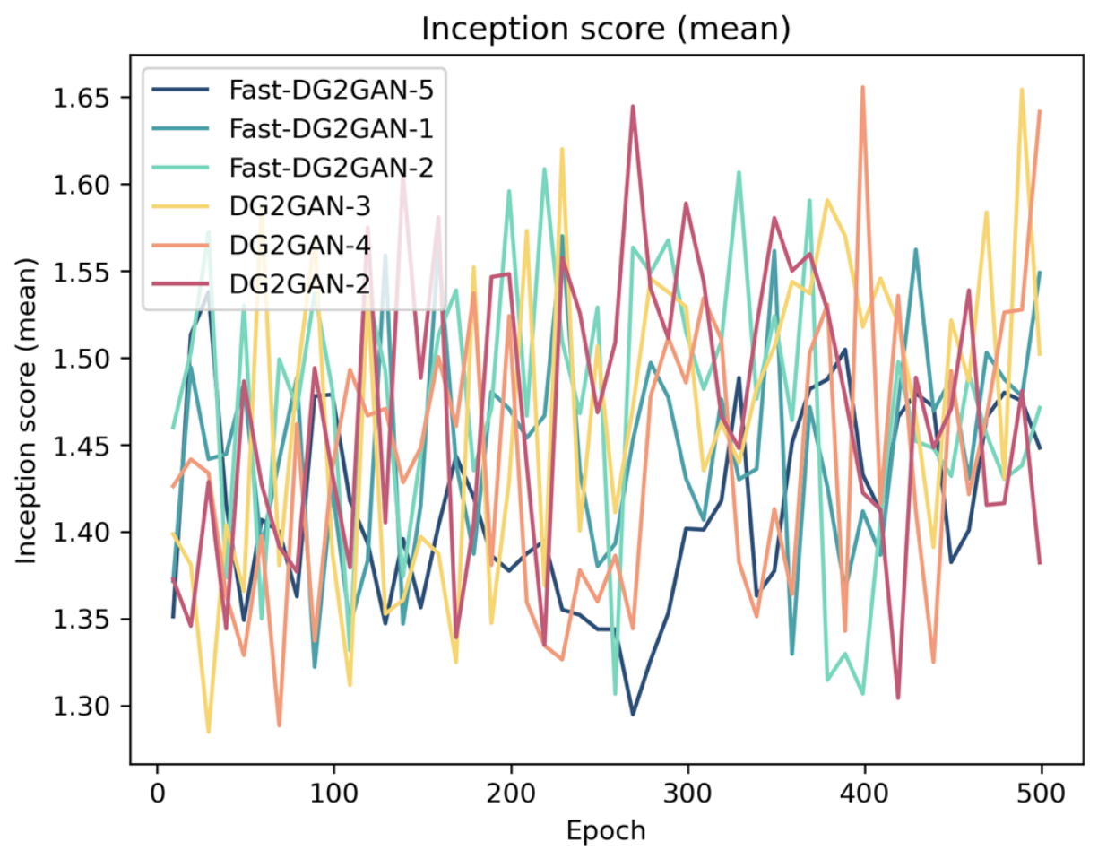

Disclaimer/Publisher’s Note: The statements, opinions and data contained in all publications are solely those of the individual author(s) and contributor(s) and not of MDPI and/or the editor(s). MDPI and/or the editor(s) disclaim responsibility for any injury to people or property resulting from any ideas, methods, instructions or products referred to in the content. |
© 2026 by the authors. Licensee MDPI, Basel, Switzerland. This article is an open access article distributed under the terms and conditions of the Creative Commons Attribution (CC BY) license.