A Human-in-the-Loop Framework for Outage Scheduling of Power Grids via LLM-RL Coordination

Abstract

As the operation modes and maintenance management requirements of power grids become increasingly complex, the optimization of monthly outage maintenance schedules faces challenges such as difficulty in multi-department coordination, high reliance on manual experience, and insufficient adaptability to dynamic demands. To address these issues, this paper proposes a collaborative optimization method for monthly outage schedules of power grids based on a large language model and reinforcement learning. The method uses the large language model to parse natural language requirements raised in balance meetings, converting requirements such as fixed maintenance dates, duration adjustments, and forbidden maintenance periods into structured constraint parameters. Subsequently, the small reinforcement learning model based on Dueling Deep Q-Network (Dueling DQN) re-optimizes the outage schedule according to the updated environment parameters, achieving a collaborative solution from meeting requirement parsing to schedule generation. Case study results on the IEEE 39-bus system show that the proposed method can integrate the dynamic requirements arising from multiple rounds of balance meetings and perform adaptive optimization of the outage schedule under different constraint conditions. Experimental results on the IEEE 39-bus system demonstrate that the proposed framework effectively optimizes monthly outage schedules. Compared with the initial schedule, the proposed method reduces monthly voltage violations by 31 times and decreases active power loss by 35.88 MWh.

1. Introduction

Monthly outage schedule optimization for transmission grids is an important part of grid operation and maintenance management. A reasonable outage schedule can reduce the impact of equipment outages on power flow distribution, voltage security, and operational economy while ensuring the smooth implementation of equipment maintenance tasks. As the construction of new power systems continues to advance, the operation modes of transmission grids become more complex, the proportion of renewable energy integration increases, and the topological couplings and operational correlations among equipment grow stronger. Outage scheduling has gradually evolved from a traditional time-arrangement problem into a complex combinatorial optimization problem with multiple objectives and multiple constraints [1,2,3,4].

In actual power grid companies, monthly outage schedules usually go through several phases: multi-department application submission, planner aggregation, preliminary scheduling, balance meeting discussions, plan revision, and final confirmation. Balance meetings are an important process for coordinating the maintenance needs of various departments and grid operation constraints. However, the requirements raised in these meetings are often dynamic and unstructured, such as adjusting the maintenance duration of a certain device, restricting the maintenance date of a certain device, or prohibiting maintenance during a specific time period. Traditional manual scheduling relies heavily on the planner’s experience. When facing a large number of outage maintenance schedules, complex equipment correlations, and dynamic demands from multiple departments, problems such as low scheduling efficiency, omission of constraints, and delayed plan adjustments often occur [5,6,7,8].

Regarding the optimization of outage schedules in power systems, existing research has mainly focused on mathematical programming, stochastic optimization, robust optimization, and heuristic search. Fu et al. [1] studied the security-constrained coordination optimization of generation and transmission outages, integrating unit maintenance, transmission line outages, unit commitment, and network security constraints into a unified optimization model. Basciftci et al. [3] investigated the joint scheduling of maintenance and operation in power systems, considering the impact of decision-dependent uncertainty on outage maintenance schedules and operational arrangements. Sadeghian et al. [4] developed a risk-averse generation outage maintenance scheduling model for combined heat and power systems, taking into account demand response and market uncertainty. Okumuşoğlu et al. [5] studied the joint scheduling of predictive maintenance and operation under fault uncertainty, co-modeling equipment failure risks and system operation decisions. Fan et al. [6] proposed a two-stage stochastic programming model for generation and transmission maintenance considering risk management, coordinating outage maintenance scheduling, operation costs, and system risk. Meanwhile, data-driven or heuristic optimization methods such as genetic algorithms, particle swarm optimization, simulated annealing, and multi-objective evolutionary algorithms have also been widely used for complex combinatorial optimization problems [9,10,11,12]. These methods have strong global search capabilities and can find feasible solutions in non-convex, non-linear, and multi-constrained problems. The above studies have improved the solution capability of outage schedule optimization from the perspectives of security constraints, uncertainty modeling, risk management, and intelligent searching. However, most of these methods still rely on pre-constructed mathematical models, encoding schemes, fitness functions, and fixed constraint handling strategies. When new business requirements such as fixed maintenance dates, forbidden maintenance periods, or adjustments to maintenance durations are raised in balance meetings, the model structure, constraint representation, or algorithm parameters usually need to be re-modified, imposing high demands on the optimization modeling and program adjustment capabilities of dispatchers. Therefore, traditional single optimization methods still suffer from insufficient field application flexibility and limited dynamic adaptability in dynamic outage scheduling scenarios driven by multiple rounds of balance meetings.

Reinforcement learning provides a new solution for sequential decision-making problems such as outage scheduling and has been applied to sequential decision-making tasks in power system operation and maintenance, as well as outage schedule optimization. Rocchetta et al. [13] constructed a reinforcement learning framework for grid operation and maintenance, incorporating a grid component health status, maintenance delays, controllable generators, and renewable energy uncertainty into the decision process to optimize grid operation and maintenance strategies. Rokhforoz et al. [14] studied the joint optimization of generator bidding and outage maintenance scheduling in competitive electricity markets, using safe multi-agent deep reinforcement learning to make outage maintenance scheduling decisions while satisfying security constraints. Lin et al. [15] addressed the uncertainty of maintenance durations in distribution networks by formulating the outage schedule adjustment process as a Markov decision process and using deep reinforcement learning to train a scheduling agent, enabling adaptive adjustments to changes in maintenance durations. Tang et al. [8] proposed an interpretable reinforcement learning method for monthly outage schedule optimization in power grids. Lee et al. [16] developed a deep reinforcement learning-based outage maintenance scheduling framework for offshore wind farm maintenance, tackling combinatorial optimization challenges arising from maintenance task allocation, weather fluctuations, and wake effects. These studies demonstrate that reinforcement learning can transform power system maintenance and outage scheduling problems into sequential decision-making processes driven by states, actions, and rewards, and is well-suited for handling continuous state changes and constraint feedback caused by adjustments to maintenance dates.

However, although existing outage scheduling algorithms can automatically complete schedule optimization under given objective functions and constraints, their optimization processes usually rely on pre-set environment parameters and structured constraints. When multiple departments raise new scheduling requirements in balance meetings, these requirements are often expressed in natural language, exhibiting characteristics of being unstructured, dynamic, and rich in business semantics. Traditional optimization algorithms and reinforcement learning environments struggle to directly understand such natural language scheduling instructions, nor can they automatically convert them into executable model parameters and scheduling constraints. Consequently, outage scheduling algorithms lack adaptive optimization capabilities when faced with dynamic requirements from multiple departments. Thus, how to enable the outage schedule optimization model to promptly understand the natural language requirements raised in balance meetings and automatically adjust the optimization environment accordingly is a key issue for improving the intelligent scheduling capability of monthly outage schedules.

In recent years, large language models (LLMs) have demonstrated strong capabilities in natural language understanding, instruction following, and structured text generation. The Transformer architecture provides important technical support for the development of modern large language models [17]. Large language models exhibit good generalization ability in few-shot learning and complex semantic understanding tasks [18]. Instruction fine-tuning based on human feedback improves the model’s ability to respond to user intentions [19]. The emergence of new reasoning models such as DeepSeek-R1 also offers greater application potential for LLMs in complex requirement parsing, rule understanding, and structured output tasks [20]. Therefore, using LLMs to parse natural language scheduling requirements from balance meetings and convert them into structured constraint parameters recognizable by outage schedule optimization models is a feasible approach to address the difficulty of adapting outage scheduling algorithms to dynamic business requirements. In the power system domain, the integration of LLMs with grid operation optimization has also begun to attract attention. Yan and Xu [21] combined a GPT-agent with deep reinforcement learning to handle real-time optimal power flow problems with linguistic stipulations. Cheng et al. [22] proposed a large language model for advanced power dispatching, exploring the application potential of LLMs in power dispatching tasks. Xiang et al. [23] studied the application of large language models in the secure operation of power systems, showing that LLMs can be used for tasks such as dispatching rule understanding, operation state analysis, and security assessment. However, LLMs themselves are not suitable as standalone solvers for strictly mathematical optimization problems, especially in transmission grid scenarios where physical constraints such as power flow convergence, voltage limits, and operational economy must be satisfied. Therefore, combining the requirement understanding capability of large language models with the numerical optimization capability of reinforcement learning models provides a new approach for solving dynamic outage schedule optimization problems.

Based on the above analysis, this paper proposes a collaborative optimization method for monthly outage schedules of transmission grids based on a large language model and reinforcement learning. The method uses the large language model to parse natural language requirements raised in balance meetings and convert them into structured constraints recognizable by the reinforcement learning environment. Subsequently, an outage schedule optimization model is constructed based on the Dueling Deep Q-Network (Dueling DQN) to generate monthly outage schedules under multiple objectives and constraints. This paper uses the IEEE 39-bus system [24] and the PYPOWER power flow calculation tool [25] for case validation, and compares the proposed method with the conventional Deep Q-Network (DQN), particle swarm optimization, and other methods to verify its effectiveness.

Although this study focuses on monthly outage scheduling, the proposed large–small model collaborative framework also has potential applications in power system security assessment, optimal power flow, and operational dispatch. By combining the requirement-understanding capability of large language models with the physically constrained optimization capability of small models, the framework can reduce the repetitive workload of dispatchers while retaining human supervision. More efficient scheduling may also reduce unnecessary power-flow redistribution and network losses, thereby supporting more sustainable power system operation.

The main contributions of this paper are as follows:

(1)

The outage scheduling problem of the transmission system is formulated as a Markov decision process and solved by Dueling DQN.

(2)

A natural language requirement parsing module is constructed and interfaced with the reinforcement learning agent for interactive optimization.

(3)

An LLM-RL collaborative model is proposed to solve the multi-objective transmission grid outage schedule optimization problem and is validated on the IEEE 39-bus system.

The remainder of this paper is organized as follows. Section 2 introduces the traditional outage schedule optimization process and establishes the outage schedule optimization model. Section 3 presents the collaborative optimization framework of the large language model and the small reinforcement learning model, including requirement parsing, JSON parameter conversion, and Markov decision process modeling. Section 4 carries out simulation validation on the IEEE 39-bus system and compares the performance of different optimization methods. Section 5 concludes the paper and discusses future research directions.

2. Outage Scheduling Optimization Model

2.1. Traditional Outage Scheduling Optimization Process

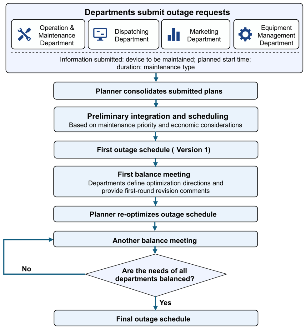
This paper focuses on monthly outage schedule optimization for transmission grids. The traditional outage schedule optimization process is shown in Figure 1. In the process of preparing monthly outage schedules in a power grid company, an outage schedule typically goes through several phases: multi-department application submission, planner aggregation, preliminary scheduling, balance meeting discussions, plan revision, and final confirmation. First, relevant departments such as the operation and maintenance department, dispatching department, marketing department, and equipment management department submit outage applications based on equipment maintenance needs. The application information usually includes the equipment to be maintained, the planned start time, the maintenance duration, and the maintenance type. Subsequently, the planner aggregates the outage schedules submitted by various departments, comprehensively considers factors such as equipment maintenance priority, grid operation safety, and economic efficiency, performs preliminary integration and scheduling, and forms the first version of the outage schedule.

In the traditional process, the balance meeting is a key step in outage schedule optimization. The first balance meeting is usually held after the preliminary scheduling is completed. Various departments propose optimization directions based on their own operational needs and grid operation constraints and form the first round of revision comments. Since the monthly outage schedule is typically prepared from the middle to the end of the previous month, the needs of various departments may change continuously during this period, and a single balance meeting is often unable to resolve all conflicts. Therefore, the planner needs to re-optimize the outage schedule based on the discussion results of the meeting. For example, some equipment may require an extended maintenance outage time, some equipment may be required to be maintained on a fixed date, or certain dates may be designated as forbidden maintenance periods. After the schedule is adjusted, another balance meeting is held to further discuss and revise the optimized schedule. The above process is iterated until the needs of all departments are basically balanced, and a final monthly outage schedule is formed.

However, the traditional outage schedule optimization process relies heavily on the planner’s manual experience and subjective judgment. Due to the large number of departments involved, complex constraints, and frequent schedule adjustments, coordination among departments is difficult, and the scheduling process is complex and tedious. In balance meetings, the dynamic requirements raised by multiple departments often need to be weighed and traded off manually by the planner, resulting in low optimization efficiency. At the same time, there are complex electrical correlations and topological couplings among transmission grid equipment. An adjustment to one outage schedule may trigger cascading changes in power flow distribution, voltage levels, and other maintenance arrangements. Faced with dynamically changing departmental needs, a large number of outage maintenance schedules, and complex grid operation constraints, traditional manual methods struggle to fully grasp the overall situation, thus limiting the efficiency and reliability of monthly outage schedule optimization.

2.2. Objective Function for Outage Scheduling

Outage scheduling requires a trade-off among grid safety, power quality, and economic efficiency. Accordingly, the optimization objective is decomposed into three sub-objectives, as defined in Equations (1)–(3).

During the preparation of the outage schedule, equipment maintenance changes the topology of the power grid. As a result, there is a risk that the power flow calculation may not converge. Since power flow analysis is fundamental to power system operation, non-convergence prevents the accurate determination of key operational parameters—such as bus voltages, phase angles, branch flows, and network losses—thereby compromising the feasibility and safety of the outage schedule. Based on this, the power flow convergence objective is formulated as:

$$\Omega \left(Flag\right)={\displaystyle \sum _{d=1}^{D_{max}}}{f}_d,$$

(1)

if $f_d=0$, the power flow calculation converged on day $d$; if $f_d=1$, the power flow calculation failed to converge on day $d$.

Reducing active power network loss is an important goal for economic operation and safety control of power systems. Taking active power loss as another optimization objective, the network loss objective function is defined as:

$$\Lambda \left(P\right)={\displaystyle \sum _{d=1}^{D_{max}}}{P}_{loss,d},$$

(2)

where $P_{loss,d}$ represents the active power loss of the lines on day $d$, obtained from the power flow calculation results.

Voltage violation poses a serious threat to both equipment safety and system stability. Reducing the number of voltage violations is an important measure to ensure safe grid operation and improve power quality. The voltage violation objective function can be expressed as:

$$\Psi \left(v\right)=\sum _{d=1}^D\sum _{i=1}^{N_b}I\left({(V}_{i,d}<0.95p.u.)\vee {(V}_{i,d}>1.05p.u.)\right),$$

(3)

where $\mathrm{I}\left(·\right)$ is defined as:

$$I\left(x\right)=\left\{\begin{array}{c}1,if \mathrm{x} \mathrm{i}\mathrm{s} \mathrm{t}\mathrm{r}\mathrm{u}\mathrm{e}\hfill \\ 0,otherwise\hfill \end{array}\right..$$

(4)

Here, $N_b$ denotes the total number of buses, $D$ represents the scheduling horizon, $V_{i,d}$ represents the voltage magnitude of bus $i$ on day $d$, and 0.95 and 1.05 p.u. are the lower and upper voltage limits, respectively.

By integrating the three objective functions presented above, the final overall optimization objective function can be expressed as:

$$F=min\left[\alpha ·\Psi \left(v\right)+\beta ·\Lambda \left(P\right)+\gamma ·\Omega \left(flag\right)\right],$$

(5)

where α, $\beta$ and $\gamma$ are weight coefficients in multi-objective optimization, used to adjust the relative importance of the three different sub-objectives in the overall objective function. In this study, the weight coefficients are set as $\mathrm{\alpha }=10$, $\mathrm{\beta }=1$, $\mathrm{\gamma }=100$ to reflect the priority of safety over economy.

2.3. Constraints for Power Grid Outage Scheduling Optimization

2.3.1. Outage Time Window Constraint

The outage window refers to a specific time period within a natural month during which maintenance of a designated device can be scheduled. The design principle is that performing device maintenance during this period minimizes the impact on grid safety and stability, power quality, and economic efficiency. Meanwhile, to improve maintenance efficiency and reasonably allocate human resources, the outage maintenance time should be continuous, and the maintenance task must be completed within a set deadline. The outage duration $T_n$ for device $\mathrm{n}$ is in days. The constraint condition for $T_n$ can be defined as:

$$t_n+T_n-1\le T_m,$$

(6)

where $t_n$ is the start date of maintenance for device $\mathrm{n}$, and $T_m$ is the set deadline.

2.3.2. Power Flow Constraint

Power flow constraints are core physical constraints that must be satisfied in the optimization of power system operation and outage maintenance schedules; they primarily include node power balance equations and branch power constraints. For any node $\mathrm{x}$ in the system, the active power balance equation is:

$$P_{G,x}-P_{M,x}=\sum _{y=1}^n{V}_x{V}_y\left(G_{xy}\mathit{cos}{\theta }_{xy}+B_{xy}\mathit{sin}{\theta }_{xy}\right),$$

(7)

the reactive power balance equation is:

$$Q_{G,x}-Q_{M,x}=\sum _{y=1}^n{V}_x{V}_y\left(G_{xy}\mathit{sin}{\theta }_{xy}-B_{xy}\mathit{cos}{\theta }_{xy}\right),$$

(8)

where $P_{G,x}$ and $Q_{G,x}$ represent the active and reactive power outputs of the generator at node $x$, respectively; $P_{M,x}$ and $Q_{M,x}$ represent the load at node $x$; $V_x$ and $V_y$ represent the voltage magnitudes at nodes $x$ and $y$, respectively; ${\theta }_{xy}$ represents the phase angle difference between the voltages at nodes $x$ and $y$; and $G_{xy}$ and $B_{xy}$ represent the conductance and susceptance of the node admittance matrix, respectively. In this study, PYPOWER(v5.x) is used to perform AC power flow calculations on the IEEE 39-bus system with MATPOWER 4.1-compatible data format [25].

2.3.3. Mandatory Maintenance Time Constraint

The mandatory maintenance time constraint is used to handle maintenance work that must be performed at a specific time due to equipment characteristics, external coordination, or other reasons. For device $n$, the constraint is:

$${\mathrm{t}}_{\mathrm{n}}={\mathrm{L}}_{\mathrm{n}},\forall n\in L,$$

(9)

where ${\mathrm{L}}_{\mathrm{n}}$ is the mandatory maintenance start time for device $n$, and $\mathrm{L}$ is the set of devices that require a fixed outage time.

2.3.4. Forbidden Maintenance Time Constraint

The forbidden maintenance time constraint is used to handle situations where no equipment maintenance is allowed during certain specific time periods. For device $n$, the constraint can be expressed as:

$$K\left(i,n\right)=1,\forall n\in U,\forall i\in {\mathrm{D}}_{\mathrm{f}\mathrm{o}\mathrm{r}\mathrm{b}\mathrm{i}\mathrm{d}},$$

(10)

where $U$ is the set of all devices to be maintained, $K\left(i,n\right)$ is the state of device $n$ on day $i$ (1 indicates normal operation, 0 indicates maintenance), and ${\mathrm{D}}_{\mathrm{f}\mathrm{o}\mathrm{r}\mathrm{b}\mathrm{i}\mathrm{d}}$ is the set of days on which maintenance is forbidden. This constraint forces that no device can be in outage maintenance status on any day within the forbidden maintenance period.

3. Large-Small Model Collaborative Optimization Framework

To improve the adaptability of monthly outage schedules for power grids to dynamic demands from multiple departments, this paper proposes an outage schedule optimization framework that integrates a large language model with reinforcement learning. The framework divides the outage scheduling process into two phases: requirement parsing and optimization solving. The large language model is responsible for understanding the natural language requirements raised by various departments in balance meetings and converting them into structured constraints. The reinforcement learning model then optimizes the outage schedule based on the updated environment parameters and constraints.

3.1. Requirement Parsing and Parameter Transformation Method Based on Large Models

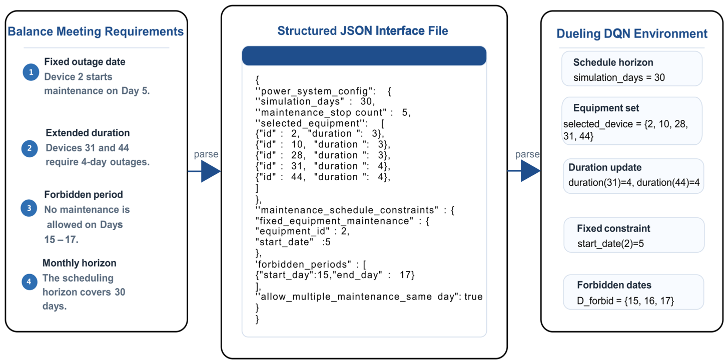
To improve the efficiency of information exchange between the large language model and the small reinforcement learning model, this paper adopts JSON format as the structured data interface. JSON organizes data using key-value pairs, offering clear structure, ease of parsing, and convenient invocation by Python programs. It is suitable for transferring constraint parameters during outage schedule optimization. Through the JSON interface, the natural language requirements parsed by the large language model can be converted into environment parameters recognizable by the small model, bridging the gap between meeting requirements and optimization model constraints. The process of large language model requirement parsing and small model environment parameter updating based on the JSON interface is shown in Figure 2.

This paper uses the web-based DeepSeek-R1 as the large language model for requirement parsing [20]. By employing a prompt template, rule constraints, and structured output examples tailored to the transmission grid outage schedule optimization scenario, the model is guided to convert natural language requirements into JSON constraint text. Specifically, the large language model first receives the balance meeting requirements organized by the planner, such as fixed maintenance dates for equipment, extended maintenance durations, and forbidden maintenance periods. It then identifies the equipment objects, time information, and constraint types, and generates a JSON file according to the predefined format.

The generated JSON file is further read by a Python parsing program and converted into parameter configurations for the reinforcement learning environment, including equipment maintenance durations, mandatory maintenance dates, forbidden maintenance dates, and feasible outage windows. The updated environment parameters are then fed into the small Dueling DQN model, which re-optimizes the outage schedule under the new constraints.

3.2. Dueling DQN Algorithm

The Deep Q-Network (DQN) is a value-based deep reinforcement learning algorithm that combines Q-learning with a deep neural network to approximate the action-value function ($Q(s,a)$) [26]. Its training framework mainly consists of an online Q-network, a target Q-network, an experience replay buffer, and an action exploration mechanism. The online Q-network estimates the Q-values of the available actions in the current state, whereas the target Q-network provides relatively stable target values for temporal-difference learning. The experience replay buffer stores state-transition samples and randomly samples mini-batches during training to reduce the temporal correlation among consecutive samples. An ε-greedy strategy is employed to balance exploration and exploitation.

As an architectural extension of DQN, the Dueling Deep Q-Network (Dueling DQN) retains the experience replay and target-network mechanisms of conventional DQN but modifies the output structure of the Q-network [27]. The Dueling Deep Q-Network (Dueling DQN) decomposes the Q-value into a state-value component and an action-advantage component. The characteristics of Dueling DQN enable the network to accurately evaluate the quality of the current state without learning the subtle differences among all action combinations, thereby achieving higher training efficiency and stability in complex action spaces. The grid outage maintenance problem studied in this paper exhibits precisely this characteristic: certain actions do not significantly affect the system state, and the Dueling structure helps the network quickly identify state transitions that offer meaningful value.

The Q-value is composed of the state value and the advantage value. The basic form is:

$$\mathrm{Q}\left(\mathrm{s},\mathrm{a};\mathrm{\theta },{\theta }_A,{\theta }_B\right)=\mathrm{V}\left(\mathrm{s};\mathrm{\theta },{\theta }_B\right)+\mathrm{A}\left(\mathrm{s},\mathrm{a};\mathrm{\theta },{\theta }_A\right),$$

(11)

where $\mathrm{s}$ represents the current state of the agent, $\mathrm{a}$ denotes the selected action, $\mathrm{\theta }$ represents the parameters of the shared feature extraction layer, ${\theta }_A$ represents the parameters of the advantage branch, and ${\theta }_B$ represents the parameters of the state-value branch. $\mathrm{V}\left(\mathrm{s};\mathrm{\theta },{\theta }_B\right)$ denotes the state-value function, which estimates the overall value of the current state regardless of the selected action. $\mathrm{A}\left(\mathrm{s},\mathrm{a};\mathrm{\theta },{\theta }_A\right)$ represents the action-advantage function, which measures the relative contribution of action a compared with other available actions under state $\mathrm{s}$.

However, the above formulation suffers from an identifiability problem because multiple combinations of $\mathrm{V}\left(\mathrm{s}\right)$ and $A\left(s,a\right)$ can produce the same Q-value. Therefore, the advantage function is normalized by subtracting its average value over all possible actions. The final Q-value estimation is formulated as:

$$\mathrm{Q}\left(\mathrm{s},\mathrm{a};\mathrm{\theta },{\theta }_A,{\theta }_B\right)=\mathrm{V}\left(\mathrm{s};\mathrm{\theta },{\theta }_B\right)+\left(\mathrm{A}\left(\mathrm{s},\mathrm{a};\mathrm{\theta },{\theta }_A\right)-{\displaystyle \frac{1}{\left|\mathcal{A}\right|}}\sum _{{\mathrm{a}}^{\prime }\in \mathcal{A}}\mathrm{A}\left(\mathrm{s},{\mathrm{a}}^{\prime };\mathrm{\theta },{\theta }_A\right)\right),$$

(12)

where $\left|\mathcal{A}\right|$ denotes the number of available actions, and ${\mathrm{a}}^{\prime }$ represents each possible action in the action space. This formulation enables the network to separately evaluate the inherent value of the current state and the relative advantage of each action, thereby improving the learning efficiency and stability of DQN in complex decision-making problems.

The loss function for Dueling DQN is the same as that for DQN (mean squared error loss). The goal is to make the estimated $Q$-values converge to the target $Q$-values $y_Q$, which are calculated according to the temporal difference (TD) objective of DQN:

$${\mathrm{y}}_{\mathrm{Q}}=\mathrm{r}+\mathrm{\gamma }·\underset{{\mathrm{a}}^{\prime }}{\max } \mathrm{Q}\left({\mathrm{s}}^{\prime },{\mathrm{a}}^{\prime };{\mathrm{\theta }}^{-}\right),$$

(13)

where $r$ represents the immediate reward received after performing action $a$, and $\mathrm{\gamma }$ is the discount factor; a larger value of $\mathrm{\gamma }$ indicates a greater preference for future rewards.

$$\mathrm{L}\left(\mathrm{\theta }\right)={\mathrm{E}}_{\left(\mathrm{s},\mathrm{a},\mathrm{r},{\mathrm{s}}^{\prime }\right)\sim \mathrm{D}}\left[{\left({\mathrm{y}}_{\mathrm{Q}}-\mathrm{Q}\left(\mathrm{s},\mathrm{a};\mathrm{\theta }\right)\right)}^2\right],$$

(14)

where $E_{\left(s,a,r,s^{\prime }\right)\sim D}$ denotes the expected value of the experience sample $\left(s,a,r,s^{\prime }\right)$, sampled from the experience replay pool $\mathrm{D}$.

3.3. Outage Schedule Optimization Decision Model Based on Dueling DQN

In the proposed collaborative framework, the small reinforcement learning model is responsible for the core optimization task. This paper builds an outage schedule optimization model based on Dueling DQN. The structured maintenance requirements parsed by the large language model are mapped into constraint parameters in the reinforcement learning environment, and scheduling optimization is performed under the updated environment. In this way, the small model can adapt to changes in maintenance requirements after balance meetings and generate a monthly outage schedule that satisfies all constraints.

3.3.1. Markov Decision Process for Outage Scheduling Optimization

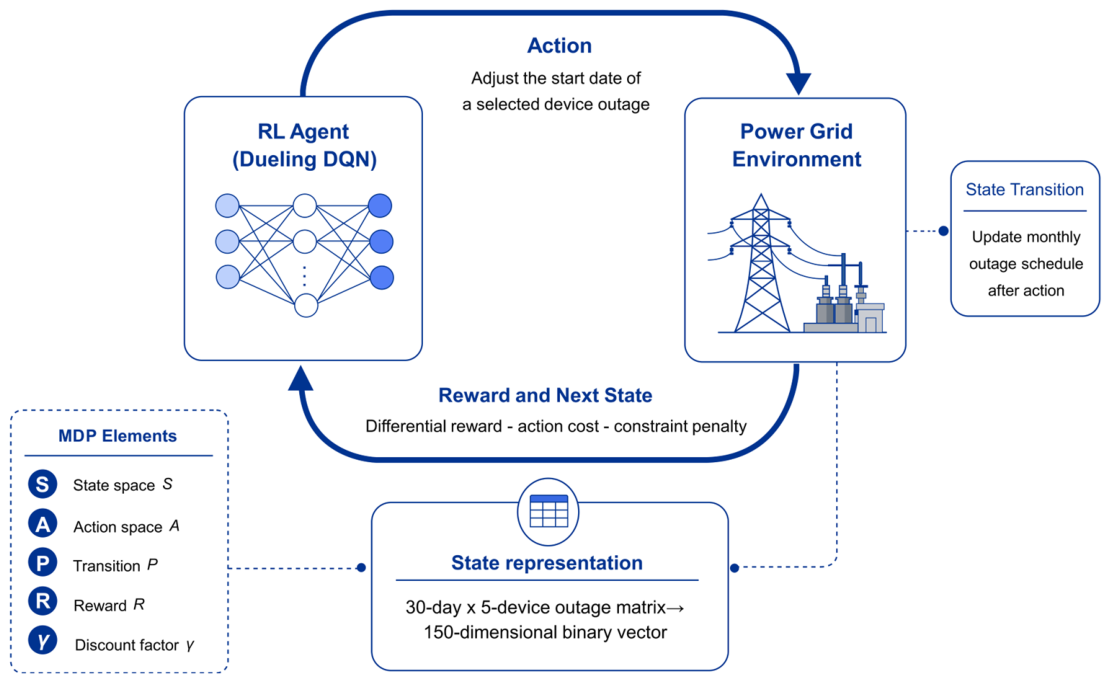
The Markov decision process (MDP) is a classical mathematical framework for modeling sequential decision-making problems under uncertainty [28]. It is suitable for modeling optimization problems characterized by state transitions and reward feedback. Its core idea is that the next state depends only on the current state and the chosen action, not on historical states or actions. An MDP is typically composed of five elements: state space, action space, state transition probability, reward function, and discount factor, denoted as $⟨S,A,P,R,\gamma ⟩$. In the optimization of transmission grid outage schedules, the outage maintenance scheduling process can be formulated as an MDP: the agent selects an adjustment action based on the current outage schedule state, the grid environment updates the outage schedule according to the action and returns a new state and reward. Based on this modeling approach, Dueling DQN can interact with the grid environment repeatedly and gradually learn an outage schedule optimization strategy that satisfies operational constraints while balancing safety and economy. Reinforcement learning has also been widely discussed as a promising tool for decision-making and control in power systems [29,30]. The MDP interaction mechanism in the outage schedule optimization process is illustrated in Figure 3.

3.3.2. State Space

The state space is a 150-dimensional binary vector, flattened row-wise from the outage maintenance schedule matrix of 30 days × 5 key devices. Each dimension takes a value of 0 or 1, where 0 indicates the device is under maintenance on that day, and 1 indicates normal operation. Let $K\left(i,n\right)$ represent the state of device $n$ on day $i$. This vector fully reflects the daily outage arrangement of the five selected devices over the next 30 days, serving as the direct input to the Dueling DQN. The state space can be expressed as:

$$s={\left(K\left(1,1\right),\dots ,K\left(1,5\right),K\left(2,1\right),\dots ,K\left(30,5\right)\right)}^{\mathrm{T}}\in {\left\{0,1\right\}}^{150}.$$

(15)

3.3.3. Action Space

In the proposed framework, the Dueling DQN agent does not output a joint action involving all maintenance devices simultaneously. Instead, a sequential decision-making strategy is adopted. At each time step, the agent selects one action from the overall discrete action space, where each action corresponds to adjusting the maintenance start date of one specific device.

The small model employs a discrete action space. For a 30-day calendar month, the action space $A_n$ for device $n$ is defined as:

$$A_n=\left[-(D_{max}-T_n),\cdots -2,-1,0,1,2\cdots ,D_{max}-T_n\right],$$

(16)

where each action represents the number of days by which the initial maintenance start date of the selected device is shifted. The overall action space is constructed by combining the adjustment operations of all maintenance devices:

$$A=\bigcup _{n=1}^{N_m}{A}_n,$$

(17)

where ${\mathrm{N}}_{\mathrm{m}}$ denotes the number of devices scheduled for maintenance.

Each action adjusts the initial maintenance date of a specific device. The adjustment is measured in days, ranging from the maximum number of days the date can be moved forward to the maximum number it can be moved backward. The maximum movable days are determined by the difference between the total number of days in the month and the maintenance duration of the device. The total dimension of the action space is the sum of the action spaces of all devices scheduled for maintenance. Through these adjustments, the agent can explore the optimal outage maintenance schedule by shifting the start dates of device outages.

3.3.4. Reward Function

In this study, a decision that meets the objectives and satisfies all constraints yields a positive reward, whereas a decision that violates constraints or deviates from the objectives incurs a corresponding penalty. After each action, the state transitions from $s_t$ to $s_{t+1}$, and the state evaluation function is expressed as:

$$F\left(s_t\right)=-\left(\alpha ·\Psi \left(v\right)+\beta ·\Lambda \left(P\right)+\gamma ·\Omega \left(flag\right)\right).$$

(18)

Let $F\left(s_t\right)=-\left(10·\Psi \left(v\right)+1·\Lambda \left(P\right)+100·\Omega \left(flag\right)\right)$, where $\Psi \left(v\right)$ is the total number of voltage violations in a natural month, $\Lambda \left(P\right)$ is the total active power network loss in the same period, and $\Omega \left(flag\right)$ is the number of days on which power flow calculation fails to converge. The coefficients 10, 1, and 100 are used to adjust the 30-day cumulative values of the three indicators to similar orders of magnitude. Typically, the number of voltage violations is in the order of hundreds, the total active power network loss is in the order of thousands of megawatts, and the number of non-convergence days is several or zero.

The system reward function $R_t$ is defined as:

$$R_t=F\left(st+1\right)-F\left(st\right)-\lambda \mid \Delta t_t\mid .$$

(19)

where $\mid \Delta t_t\mid$ represents the scheduling adjustment caused by the action selected at step $t$, which is defined as:

$$\Delta t_t=t_t^{new}-t_t^{old},$$

(20)

where $t_t^{old}$ denotes the maintenance scheduling date before executing the action at step $\mathrm{t}$, $t_t^{new}$ represents the updated maintenance scheduling date after executing the action, and $\mid \Delta t_t\mid$ represents the magnitude of the scheduling adjustment. $\lambda$ is the penalty coefficient for the movement cost.

This reward design adopts a differential form, aiming to directly measure the improvement in the state evaluation function resulting from a single action. If $F\left(st+1\right)>F\left(st\right)+\lambda \mid \Delta t_t\mid$, the reward is positive; otherwise, a penalty is applied. In addition, the movement cost term $\mathrm{\lambda }\mid \Delta t_t\mid$ is introduced as an action adjustment penalty, encouraging the agent to achieve better scheduling performance with fewer unnecessary modifications. This design ensures that the cumulative reward over an entire episode reflects the improvement of the final state evaluation value relative to the initial state while considering the cost of schedule adjustments, thereby balancing system performance improvement and plan modification costs.

When the agent selects an action that violates the rules, that step directly returns a fixed penalty value. Penalties fall into three categories: adjusting a fixed maintenance device, scheduling during a prohibited maintenance date, or extending the maintenance window beyond the bounds of a calendar month. In such cases, the reward function is not computed, and the agent remains in the state $s_t$ from the end of the previous step.

3.4. Collaborative Optimization Process of Large and Small Models

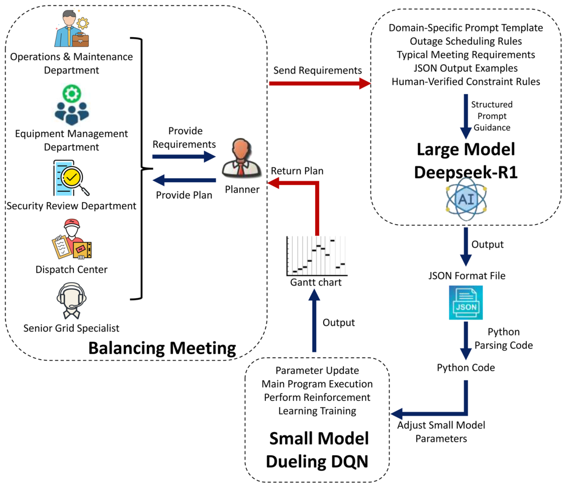
Traditional outage schedule planning for transmission grids relies mainly on manual experience. In multi-department collaborative decision-making scenarios, manual planning not only suffers from low adjustment efficiency and slow update speed but also struggles to fully account for the electrical correlations and topological couplings among equipment, as well as the interactions between different outage schedules. When the outage time of one device changes, it may trigger cascading effects on power flow distribution, voltage levels, and other maintenance arrangements, increasing the risk of constraint omissions and misjudgments. Meanwhile, traditional optimization algorithms usually depend on fixed model parameters and constraints, making them poorly adaptable to the constantly changing maintenance requirements that emerge after balance meetings, and thus unable to meet the need for rapid schedule adjustments in practice. To address these issues, this paper proposes a collaborative optimization method for transmission grid outage schedules that integrates a large language model with a small reinforcement learning model. The overall framework is illustrated in Figure 4.

In this collaborative framework, the large language model is primarily responsible for requirement parsing and constraint generation. This paper uses the web-based DeepSeek-R1 [20] to parse the unstructured maintenance requirements raised by various departments during balance meetings, such as extended maintenance durations, forbidden maintenance on specific dates, and fixed maintenance dates for certain equipment. Subsequently, following a preset prompt template and structured output rules, the large language model converts these requirements into constraint parameters in JSON format, which are then input as environment configurations for the small reinforcement learning model. The small reinforcement learning model, based on the Dueling DQN algorithm, performs outage schedule optimization under the updated constraint environment, generating a monthly outage schedule that satisfies both maintenance requirements and operational constraints. In this way, the large language model handles natural language requirement understanding and structured constraint conversion, while the small reinforcement learning model undertakes multi-constraint scheduling optimization. Together, they achieve a closed-loop connection from balance meeting requirements to optimized outage schedules, thereby improving the adaptability to dynamic requirements and the optimization efficiency of monthly outage schedules for transmission grids.

It should be noted that the proposed framework is intended for planning-level monthly outage scheduling rather than direct real-time operational control. Monthly outage schedules are generally prepared and iteratively revised over several days following balance meetings; therefore, sufficient computation time is available, and data latency and computational burden are not primary constraints in the present application. However, these issues, together with integration into existing utility IT infrastructure, must be further addressed when the framework is extended to real-time applications such as optimal power flow.

4. Experimental Simulation

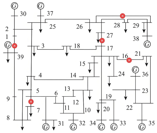
To verify the effectiveness of the proposed method, a case study with different phases is conducted on the IEEE 39-bus system. The first phase is the basic optimization phase, where outage scheduling is optimized solely using a small reinforcement learning model. The second phase simulates schedule adjustments after the first round of balancing meetings: a large language model interprets the newly added requirements and updates the environmental parameters of the reinforcement learning model. The third phase further introduces dynamic constraints after a second round of balancing meetings to validate the method’s adaptability to multi-round changes in requirements. The IEEE 39-bus system is a standard test system commonly used in power system research, consisting of 39 buses, 10 generators, and 46 branches. In this study, AC power flow calculations are performed using PYPOWER. Equipment 2, 10, 28, 31, and 44 are selected as the units to be maintained, and the scheduling horizon is set to 30 days, i.e., $D_{\mathrm{m}\mathrm{a}\mathrm{x}}=30$. The outage maintenance topology of the IEEE 39-bus system is shown in Figure 5, where the branches marked are the equipment to be maintained in this paper. In the IEEE 39-bus system, the numbering of maintenance devices follows the corresponding transmission branch indices. It should be noted that a transmission branch may contain multiple physical devices, and the outage of any critical device within the branch may require the branch to be removed from service during maintenance.

4.1. Outage Scheduling Optimization Experiment with the Small Model

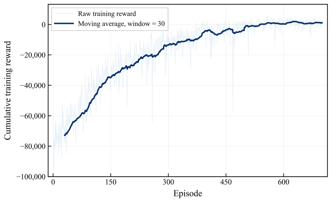
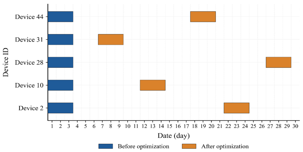
The large model plays the role of adjusting the reinforcement learning environment parameters of the small model. When optimizing the initial outage schedule submitted at the beginning of the month without holding a balance meeting, the small model can complete the task independently; this phase is defined as Phase 1. In Phase 1, when scheduling outages for the five devices (2, 10, 28, 31, and 44), the outage maintenance duration $T_n$ is uniformly set to three consecutive days. The initial state is configured such that all five devices undergo maintenance in the first three days. The training process involves 700 episodes, with an initial exploration rate of 1.0, an initial learning rate of 0.0005, and 100 steps per episode.

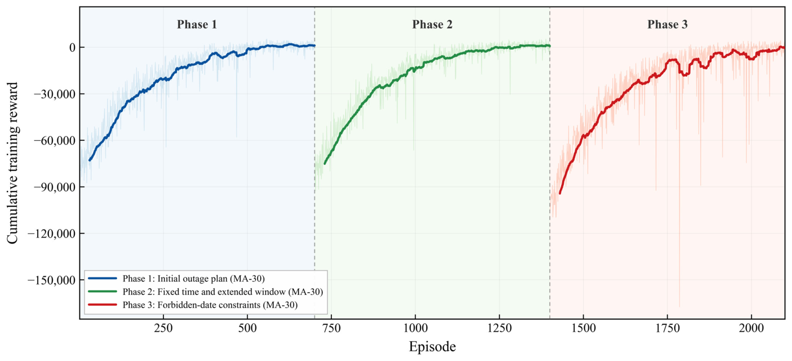
Figure 6 shows the total reward curve during the training process for the initial outage schedule in Phase 1. Overall, the reward starts from a negative value below −80,000 at the beginning of training and exhibits a sustained and significant upward trend as episodes increase. The increase is rapid in the early phases, gradually slows down, and eventually stabilizes, converging to a range near zero. This trend indicates that the agent transitions from an ineffective strategy to gradually learning effective decision-making in the task of initial outage schedule optimization, demonstrating that the algorithm achieves good learning efficiency and convergence in this scenario. The small model is the core component of outage schedule optimization and is capable of completing the entire training process on its own.

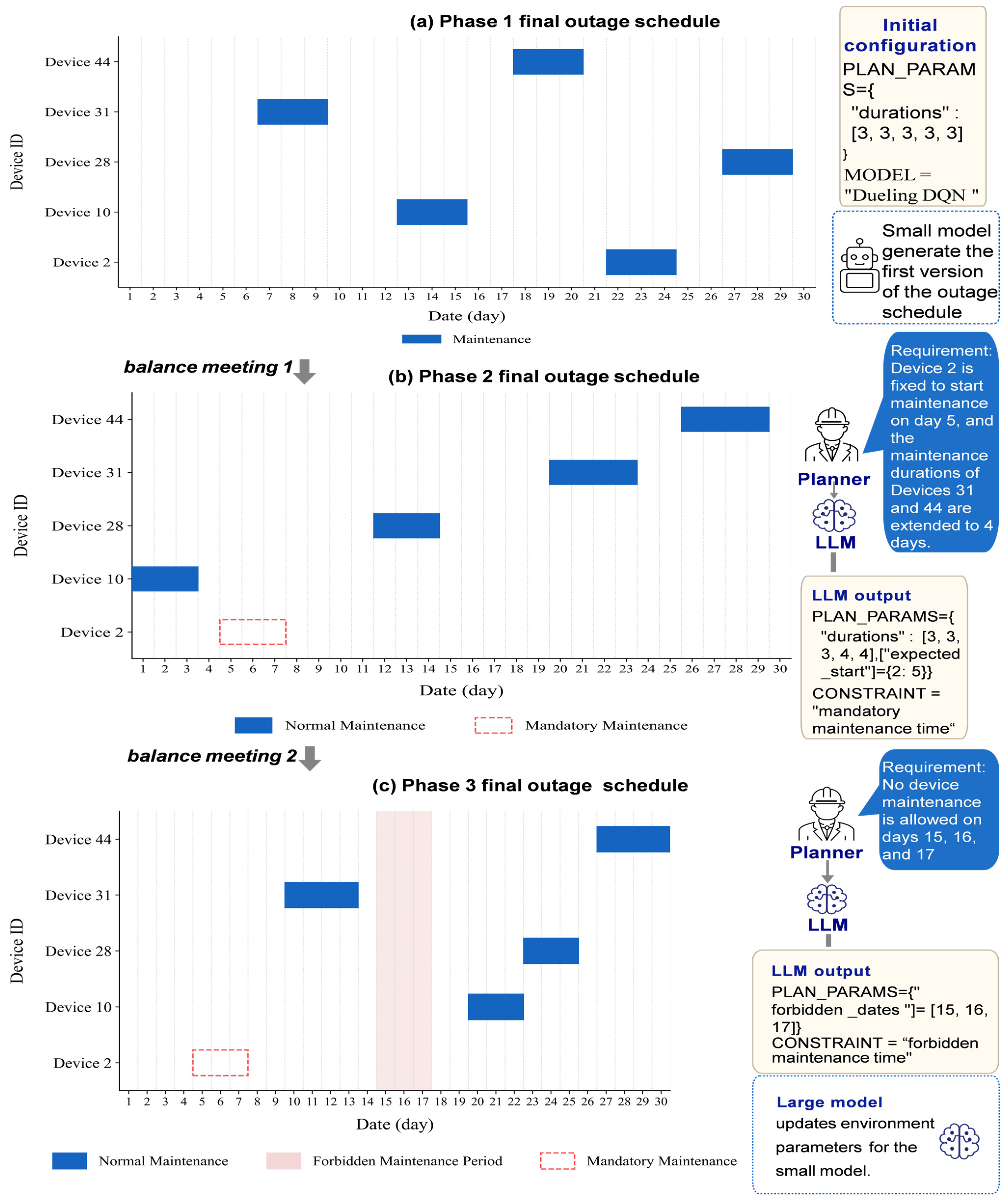
Figure 7 shows the Gantt chart comparison before and after outage schedule optimization in Phase 1. The horizontal axis represents the date, and the vertical axis represents the equipment number. In the initial state, the outage maintenance of the five devices is all concentrated in the first three days. Multiple devices being out of service simultaneously can easily cause significant changes in power flow distribution and increase the risk of voltage violations. After optimization by the small model, the maintenance times of the devices are distributed throughout the month, and the outage times of different devices are staggered. This reduces the impact of concentrated maintenance on system operation and facilitates the rational allocation of maintenance resources and personnel. This result shows that, in Phase 1 where only the small model participates in optimization, Dueling DQN can initially adjust the time distribution of the outage schedule and improve the rationality of outage arrangements.

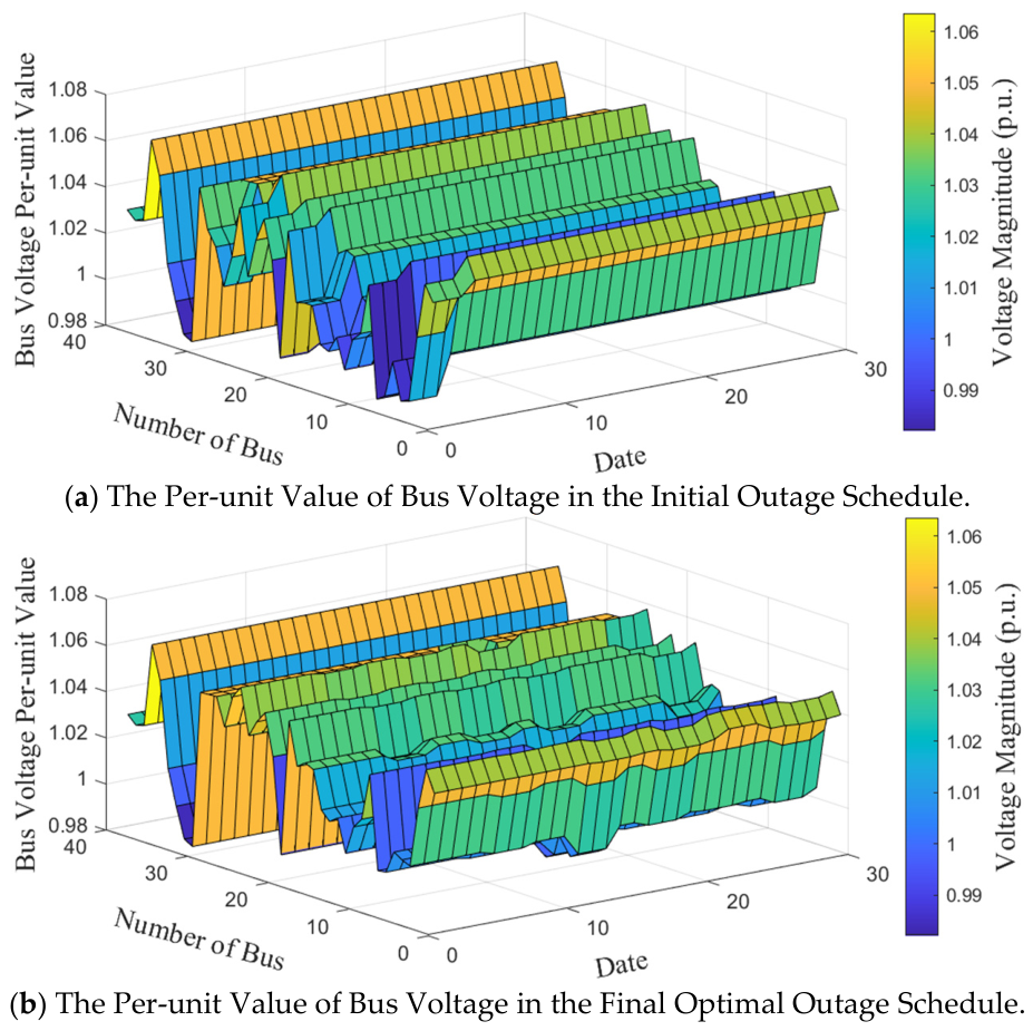
Figure 8 compares the per-unit voltage variations in each bus in the IEEE 39-bus system under the initial outage maintenance schedule of Phase 1 and the final optimized outage maintenance schedule. Figure 8a shows the bus voltage distribution under the initial schedule, and Figure 8b shows the bus voltage distribution under the final optimized schedule. It can be observed that, under the initial schedule, voltage fluctuations on some days and at some buses are relatively obvious, and certain local areas exhibit voltages close to or exceeding the safety limits, indicating that concentrated outage maintenance has a significant impact on system voltage stability. After optimization, the overall bus voltage distribution becomes more stable, abnormal voltage fluctuations are reduced, and the system voltage operation status is improved. Statistical results show that the total number of voltage violations after optimization decreases by 33, demonstrating that the proposed method can mitigate the impact of outage maintenance on voltage security by adjusting device maintenance periods, thereby improving the safety and rationality of the monthly outage schedule.

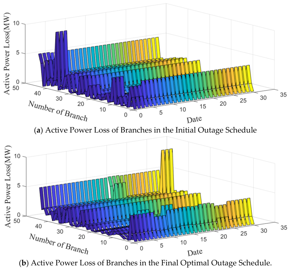
Figure 9 compares the changes in branch active power network loss under the initial outage maintenance schedule of Phase 1 and the final optimized outage maintenance schedule. Figure 9a shows the branch active power network loss distribution under the initial schedule, and Figure 9b shows the distribution under the final optimized schedule. In the figure, the horizontal axis represents the date, the vertical axis represents the branch number, and the (z)-axis represents the instantaneous average active power network loss of the branch on the corresponding date. It can be observed that, under the initial schedule, the active power network loss on some dates and branches is relatively high, indicating that concentrated equipment outages cause power flow redistribution and lead to increased local branch losses. After optimization, the distribution of high-loss areas becomes more dispersed, and the overall level of active power network loss is reduced. This shows that the optimized maintenance schedule can more reasonably arrange equipment outage periods, mitigating the impact of concentrated maintenance on system operational economy. Statistical results show that the total monthly active power network loss of the final optimized schedule is reduced by 41.23 MWh compared with the initial schedule, demonstrating that the proposed method can effectively improve system operational economy while satisfying maintenance constraints.

4.2. Outage Scheduling Optimization Experiment with Large-Small Model Collaboration

The IEEE 39-bus system was again selected for the experiment. After Phase 1 concluded, the departments held their first balance meeting, during which the following new requirements were identified: Device 2 can only undergo maintenance starting on Day 5; the outage time windows for Devices 31 and 44 are extended to four days. The large model converted the new natural language requirements summarized by the planners into a JSON file and transmitted it to the small model. The small model parsed the JSON file using a parsing code to obtain Python code for the reinforcement learning environment parameters. Following these steps, Phase 2 training was conducted for 700 episodes, with an initial exploration rate of 1.0, an initial learning rate of 0.0005, and 100 steps per episode. After Phase 2 training, the departments held a second balance meeting, adding a new requirement to the previous ones: no device maintenance is permitted on days 15, 16, and 17. The process was repeated, and Phase 3 reinforcement learning training was performed.

All experiments were conducted on a workstation equipped with an NVIDIA GeForce GTX 1650 GPU. The training times for Phases 1, 2, and 3 were approximately 2.30, 2.50, and 2.75 h, respectively, resulting in a total training time of approximately 7.55 h. After training, the average neural network inference time required to select a single scheduling action was approximately 1.8 ms. The generation and validation of a complete monthly outage schedule, including the associated AC power-flow calculations, required approximately 18.5 s. Since monthly outage scheduling is an offline or near-offline planning task conducted after balance meetings, the above computational time is acceptable for the IEEE 39-bus system considered in this study.

Figure 10 illustrates the cumulative training reward trends during the outage schedule optimization process across the different phases. It can be observed that the cumulative rewards in all different phases gradually increase with the number of training episodes and eventually stabilize, indicating that the small model can progressively learn effective scheduling strategies under different constraint conditions. Compared with Phase 1, Phases 2 and 3 have lower initial rewards and more pronounced fluctuations due to the introduction of additional constraints such as fixed maintenance times, extended equipment maintenance durations, and forbidden maintenance dates. However, after training, they still converge to a relatively high level. This result demonstrates that the proposed method has good learning ability and adaptability in multi-phase dynamic constraint scenarios.

Figure 11 presents the final outage scheduling results obtained after optimization across the different phases. Figure 11a presents the outage schedule obtained in Phase 1, where only the small reinforcement learning model performs optimization independently. At this phase, no new constraints from balance meetings are introduced, and the model primarily completes the optimization of equipment outage periods based on the initial maintenance parameters. Figure 11b shows the optimization result after the first balance meeting. The large language model parses the requirements raised in the meeting, such as fixed maintenance dates and adjustments to maintenance durations, and converts them into structured constraint parameters, which are then used to update the small model environment. As a result, the optimized outage schedule can satisfy new requirements such as the fixed maintenance of Device 2. Figure 11c shows the final optimization result after the second balance meeting. On the basis of the previous phase, forbidden maintenance period constraints are further introduced. In the figure, the light red areas indicate forbidden maintenance dates, and the red dashed boxes indicate mandatory maintenance arrangements. It can be seen that as the balance meeting requirements are gradually introduced, the large language model can convert unstructured meeting requirements into constraints recognizable by the small model. The small model then re-optimizes the schedule in the updated environment, ultimately generating a monthly outage schedule that simultaneously satisfies the requirements of fixed maintenance, forbidden maintenance, and maintenance durations.

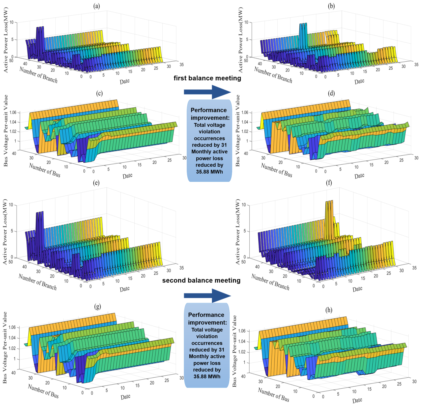
Figure 12 compares the branch active power loss and bus voltage profiles under different outage maintenance optimization phases. The left subfigures correspond to the initial or previous-phase schedules, and the right subfigures show the results after the LLM interprets updated balance meeting requirements and the Dueling DQN re-optimizes the outage schedule.

In the initial schedules, several maintenance tasks are concentrated within the same period, causing multiple transmission branches to be simultaneously unavailable. This increases power transfer stress on the remaining branches and leads to higher active power losses and voltage deviations in the IEEE 39-bus system. After optimization, the proposed framework redistributes outage periods, alleviating the impact of concentrated maintenance on power flow distribution and voltage profiles. The optimized schedules reduce voltage violations by 31 times and decrease the monthly active power loss by 35.88 MWh while satisfying the updated maintenance constraints, demonstrating improved operational safety and economic performance.

4.3. Comparative Analysis of Optimization Algorithms

Table 1. Comparison of optimization performance in different phases.

Method	Phase 1 Reward	Phase 1 Invalid Decisions	Phase 2 Reward	Phase 2 Invalid Decisions	Phase 3 Reward	Phase 3 Invalid Decisions
LLM + PSO	−154	2	−1145	6	−2759	7
LLM + DQN	940	0	708	1	−875	3
LLM + Dueling DQN	1137	0	793	0	−651	0

compares the optimization performance of three methods, namely LLM + PSO, LLM + DQN, and LLM + Dueling DQN, across the different phases. To ensure a fair comparison, all three methods use the same IEEE 39-bus system, maintenance equipment, dynamic requirements, reward function, and constraint settings; the only difference lies in the optimization algorithm. The values in the table represent the average reward over the last 30 episodes of each phase. It should be noted that PSO is not a reinforcement learning algorithm; therefore, its reward value is the evaluation result obtained by substituting the candidate schedules generated during the search process into the same reward function used for the reinforcement learning methods. The number of invalid decisions indicates how many times the schedule adjustment actions generated or executed by each method violated outage schedule constraints within the same statistical window.

It should be noted that the cumulative reward is an internal learning signal rather than the final optimization metric. Since the reward includes both performance improvement rewards and penalties for infeasible actions, negative cumulative rewards may occur when the agent explores constraint-violating actions during dynamic optimization. Therefore, the final scheduling performance is evaluated based on operational indicators rather than reward values alone.

From Table 1, it can be seen that LLM + Dueling DQN achieves the highest average reward values in all different phases, which are 1137, 793, and −651, respectively, and the number of invalid decisions is zero in all different phases. This indicates that the proposed method has good optimization effectiveness and constraint adaptability under different dynamic constraints. In contrast, LLM + PSO obtains lower average reward values, and as the constraint complexity increases, the number of invalid decisions gradually increases, indicating insufficient search stability in complex dynamic constraint scenarios. LLM + DQN performs better than LLM + PSO but is still inferior to LLM + Dueling DQN in terms of average reward value and constraint satisfaction capability. Overall, as constraints such as fixed maintenance and forbidden maintenance are gradually introduced, the optimization difficulty for all methods increases. Nevertheless, the proposed LLM + Dueling DQN method maintains a relatively high average reward level while avoiding invalid decisions, verifying its effectiveness in multi-phase outage schedule optimization.

5. Conclusions

This paper addresses the challenges in monthly outage schedule optimization for transmission grids, including difficulty in multi-department coordination, strong reliance on manual experience, and poor adaptability to dynamic requirements in a timely manner. A collaborative outage schedule optimization method based on a large language model and a small reinforcement learning model is proposed. The large language model is used to parse unstructured maintenance requirements raised in balance meetings and convert them into structured constraint parameters recognizable by the reinforcement learning environment. Subsequently, an outage schedule optimization model is constructed based on Dueling DQN, where the monthly outage scheduling process is formulated as a Markov decision process. Taking power flow convergence, number of voltage violations, and active power network loss as optimization objectives, the method optimizes the outage schedule under multiple constraints.

The IEEE 39-bus case study demonstrates that the proposed framework can effectively handle multi-phase dynamic constraint updates. Compared with the initial outage schedule, first-stage optimization reduces the monthly total voltage violations by 33 times and decreases active power loss by 41.23 MWh. After further constraint updates, the second and third optimization phases achieve reductions of 31 voltage violations and 35.88 MWh active power loss, respectively.

Case study results on the IEEE 39-bus system show that the proposed method can effectively adapt to dynamic requirements arising from multiple rounds of balance meetings and re-optimize the outage schedule under different constraint conditions. Compared with the initial schedule, the optimized outage schedule reduces the number of voltage violations and lowers the monthly active power network loss, demonstrating that the method is effective in improving the safety and economy of transmission grid operation. Furthermore, comparative experimental results show that Dueling DQN achieves higher reward values and fewer invalid decisions than PSO and traditional DQN during the optimization process across the different phases, verifying the effectiveness and feasibility of the proposed collaborative optimization framework.

Future research may focus on locally deploying the large language model, pre-training it, and constructing a dedicated knowledge base and rule base for transmission grid outage schedule optimization. In addition, the proposed framework will be further validated on very large-scale power grids, with emphasis on improving scalability through parallel power-flow computation and hierarchical or regional decomposition. Future research will also investigate more efficient constraint-handling mechanisms, such as adaptive action masking and constrained reinforcement learning, to reduce infeasible exploration and improve training efficiency. Furthermore, the integration of the proposed framework with existing utility IT infrastructure will be investigated. This will require standardized data interfaces with operational and maintenance management systems, secure data exchange, access control, and traceable decision records.

References

1. Fu, Y.; Shahidehpour, M.; Li, Z. Security-Constrained Optimal Coordination of Generation and Transmission Maintenance Outage Scheduling. IEEE Trans. Power Syst. 2007, 22, 1302–1313. [Google Scholar] [CrossRef]
2. Froger, A.; Gendreau, M.; Mendoza, J.E.; Pinson, É.; Rousseau, L.-M. Maintenance Scheduling in the Electricity Industry: A Literature Review. Eur. J. Oper. Res. 2016, 251, 695–706. [Google Scholar] [CrossRef]
3. Basciftci, B.; Ahmed, S.; Gebraeel, N. Data-Driven Maintenance and Operations Scheduling in Power Systems under Decision-Dependent Uncertainty. IISE Trans. 2020, 52, 589–602. [Google Scholar] [CrossRef]
4. Sadeghian, O.; Mohammadpour Shotorbani, A.; Mohammadi-Ivatloo, B.; Sadiq, R.; Hewage, K. Risk-Averse Maintenance Scheduling of Generation Units in Combined Heat and Power Systems with Demand Response. Reliab. Eng. Syst. Saf. 2021, 216, 107960. [Google Scholar] [CrossRef]
5. Okumuşoğlu, B.C.; Basciftci, B.; Kocuk, B. An Integrated Predictive Maintenance and Operations Scheduling Framework for Power Systems under Failure Uncertainty. Inf. J. Comput. 2024, 36, 1335–1358. [Google Scholar] [CrossRef]
6. Fan, A.; Huang, Z.; Zheng, Q.; Luo, X. A Two-Stage Stochastic Programming Approach for Generation and Transmission Maintenance Scheduling with Risk Management. Comput. Optim. Appl. 2025, 92, 787–809. [Google Scholar] [CrossRef]
7. Liu, H.; Jiang, Q.; Gui, Q.; Wang, L.; Tian, H.; Wang, J.; Yang, H. Optimal Decision-Making Model for Power Grid Maintenance Scheduling Considering Comprehensive Supply-Demand Factors. Electr. Power 2021, 54, 159–167. (In Chinese) [Google Scholar] [CrossRef]
8. Tang, W.; Mao, X.; Lv, K.; Cai, Z.; Ding, Z. Monthly Power Outage Maintenance Scheduling for Power Grids Based on Interpretable Reinforcement Learning. Energies 2025, 18, 5454. [Google Scholar] [CrossRef]
9. Holland, J.H. Adaptation in Natural and Artificial Systems; University of Michigan Press: Ann Arbor, MI, USA, 1975. [Google Scholar]
10. Kennedy, J.; Eberhart, R. Particle Swarm Optimization. In Proceedings of the IEEE International Conference on Neural Networks, Perth, Australia, 27 November–1 December 1995; Volume 4, pp. 1942–1948. [Google Scholar] [CrossRef]
11. Deb, K.; Pratap, A.; Agarwal, S.; Meyarivan, T. A Fast and Elitist Multiobjective Genetic Algorithm: NSGA-II. IEEE Trans. Evol. Comput. 2002, 6, 182–197. [Google Scholar] [CrossRef]
12. Kirkpatrick, S.; Gelatt, C.D.; Vecchi, M.P. Optimization by Simulated Annealing. Science 1983, 220, 671–680. [Google Scholar] [CrossRef] [PubMed]
13. Rocchetta, R.; Bellani, L.; Compare, M.; Zio, E.; Patelli, E. A Reinforcement Learning Framework for Optimal Operation and Maintenance of Power Grids. Appl. Energy 2019, 241, 291–301. [Google Scholar] [CrossRef]
14. Rokhforoz, P.; Montazeri, M.; Fink, O. Safe Multi-Agent Deep Reinforcement Learning for Joint Bidding and Maintenance Scheduling of Generation Units. Reliab. Eng. Syst. Saf. 2023, 232, 109081. [Google Scholar] [CrossRef]
15. Lin, M.; Wang, X.; Dou, J.; Qiao, J.; Liu, Z.; Han, Y.; Li, Y. Research on Adaptive Scheduling Method Based on DRL for Distribution Network Maintenance Durations Uncertainty. In Proceedings of the 11th Frontier Academic Forum of Electrical Engineering; Yang, Q., Li, J., Eds.; Lecture Notes in Electrical Engineering; Springer: Singapore, 2025; Volume 1291, pp. 153–160. [Google Scholar] [CrossRef]
16. Lee, N.; Woo, J.; Kim, S. A Deep Reinforcement Learning Ensemble for Maintenance Scheduling in Offshore Wind Farms. Appl. Energy 2025, 377, 124431. [Google Scholar] [CrossRef]
17. Vaswani, A.; Shazeer, N.; Parmar, N.; Uszkoreit, J.; Jones, L.; Gomez, A.N.; Kaiser, Ł.; Polosukhin, I. Attention Is All You Need. In Advances in Neural Information Processing Systems; Curran Associates, Inc.: Red Hook, NY, USA, 2017; Volume 30. [Google Scholar]
18. Brown, T.; Mann, B.; Ryder, N.; Subbiah, M.; Kaplan, J.D.; Dhariwal, P.; Neelakantan, A.; Shyam, P.; Sastry, G.; Askell, A.; et al. Language Models Are Few-Shot Learners. In Advances in Neural Information Processing Systems; Curran Associates, Inc.: Red Hook, NY, USA, 2020; Volume 33, pp. 1877–1901. [Google Scholar]
19. Ouyang, L.; Wu, J.; Jiang, X.; Almeida, D.; Wainwright, C.L.; Mishkin, P.; Zhang, C.; Agarwal, S.; Slama, K.; Ray, A.; et al. Training Language Models to Follow Instructions with Human Feedback. In Advances in Neural Information Processing Systems; Curran Associates, Inc.: Red Hook, NY, USA, 2022; Volume 35, pp. 27730–27744. [Google Scholar]
20. Guo, D.; Yang, D.; Zhang, H.; Song, J.; Wang, P.; Zhu, Q.; Xu, R.; Zhang, R.; Ma, S.; Bi, X.; et al. DeepSeek-R1: Incentivizing Reasoning Capability in LLMs via Reinforcement Learning. arXiv 2025, arXiv:2501.12948. [Google Scholar] [CrossRef]
21. Yan, Z.; Xu, Y. Real-Time Optimal Power Flow with Linguistic Stipulations: Integrating GPT-Agent and Deep Reinforcement Learning. IEEE Trans. Power Syst. 2024, 39, 4747–4750. [Google Scholar] [CrossRef]
22. Cheng, Y.; Zhao, H.; Zhou, X.; Zhao, J.; Cao, Y.; Yang, C.; Cai, X. A Large Language Model for Advanced Power Dispatch. Sci. Rep. 2025, 15, 8925. [Google Scholar] [CrossRef] [PubMed]
23. Xiang, Y.; Tan, L.; Qiu, G.; Tang, Z.; Liu, J. Large Language Model for Secure Operation of Power Systems. Smart Energy Syst. Res. 2025, 1, 10005. [Google Scholar] [CrossRef]
24. Athay, T.; Podmore, R.; Virmani, S. A Practical Method for the Direct Analysis of Transient Stability. IEEE Trans. Power Appar. Syst. 1979, PAS-98, 573–584. [Google Scholar] [CrossRef]
25. Zimmerman, R.D.; Murillo-Sánchez, C.E.; Thomas, R.J. MATPOWER: Steady-State Operations, Planning, and Analysis Tools for Power Systems Research and Education. IEEE Trans. Power Syst. 2011, 26, 12–19. [Google Scholar] [CrossRef]
26. Mnih, V.; Kavukcuoglu, K.; Silver, D.; Rusu, A.A.; Veness, J.; Bellemare, M.G.; Graves, A.; Riedmiller, M.; Fidjeland, A.K.; Ostrovski, G.; et al. Human-level control through deep reinforcement learning. Nature 2015, 518, 529–533. [Google Scholar] [CrossRef] [PubMed]
27. Wang, Z.; Schaul, T.; Hessel, M.; van Hasselt, H.; Lanctot, M.; de Freitas, N. Dueling network architectures for deep reinforcement learning. In Proceedings of the 33rd International Conference on Machine Learning, New York, NY, USA, 20–22 June 2016; Balcan, M.F., Weinberger, K.Q., Eds.; Proceedings of Machine Learning Research; PMLR: New York, NY, USA, 2016; Volume 48, pp. 1995–2003. [Google Scholar]
28. Puterman, M.L. Markov Decision Processes: Discrete Stochastic Dynamic Programming; John Wiley & Sons: New York, NY, USA, 1994. [Google Scholar] [CrossRef]
29. Chen, X.; Qu, G.; Tang, Y.; Low, S.; Li, N. Reinforcement Learning for Selective Key Applications in Power Systems: Recent Advances and Future Challenges. IEEE Trans. Smart Grid 2022, 13, 2935–2958. [Google Scholar] [CrossRef]
30. Pesántez, G.; Guamán, W.; Córdova, J.; Torres, M.; Benalcazar, P. Reinforcement Learning for Efficient Power Systems Planning: A Review of Operational and Expansion Strategies. Energies 2024, 17, 2167. [Google Scholar] [CrossRef]
Figure 1. Flowchart of the traditional outage scheduling optimization process.
Machines 14 00860 g001
Figure 2. JSON-based constraint interface for outage scheduling.
Machines 14 00860 g002
Figure 3. MDP-based interaction mechanism for Dueling DQN outage scheduling optimization.
Machines 14 00860 g003
Figure 4. Collaborative optimization framework of the large and small models for outage scheduling.
Machines 14 00860 g004
Figure 5. Outage maintenance topology of the IEEE 39-bus system. The red cross symbols mark the five transmission branches selected for outage maintenance, the black downward arrows denote loads, and the circles labeled “G” represent generators.
Machines 14 00860 g005
Figure 6. Total reward trend during outage scheduling optimization using only the small model in Phase 1.
Machines 14 00860 g006
Figure 7. Comparison of outage schedules before and after optimization in Phase 1.
Machines 14 00860 g007
Figure 8. Bus voltage magnitudes of the IEEE 39-bus system under the initial and optimized Phase 1 outage schedule.
Machines 14 00860 g008
Figure 9. Active power losses per branch of the IEEE 39-bus system under the initial and optimized Phase 1 outage schedule.
Machines 14 00860 g009
Figure 10. Comparison of cumulative training rewards across the three phases. The light-colored curves represent the raw training rewards, whereas the dark-colored curves represent the moving-average rewards calculated using a window of 30 episodes.
Machines 14 00860 g010
Figure 11. The final outage schedules for the different phases. The gray arrows indicate the sequential flow of information and schedule updates, including the transition between successive balance-meeting phases and the transfer of requirements and parameters among the planner, the LLM, and the scheduling model.
Machines 14 00860 g011
Figure 12. Comparison of branch active power loss distributions and bus voltage profiles before and after re-optimization in Phases 2 and 3: (a) branch active power loss distribution before Phase 2 re-optimization; (b) branch active power loss distribution after Phase 2 re-optimization; (c) bus voltage profile before Phase 2 re-optimization; (d) bus voltage profile after Phase 2 re-optimization; (e) branch active power loss distribution before Phase 3 re-optimization; (f) branch active power loss distribution after Phase 3 re-optimization; (g) bus voltage profile before Phase 3 re-optimization; (h) bus voltage profile after Phase 3 re-optimization.
Machines 14 00860 g012