Transient FSI–Fatigue Coupling Analysis of a Francis Turbine Runner Under Load Rejection

Abstract

With increasing renewable energy penetration, hydropower units face more frequent load rejection transients, which impose severe hydraulic excitation on Francis turbine runners. Although extensive studies have investigated flow dynamics and stress concentrations during transients, quantitative fatigue damage assessments for runners with pre-existing cracks remain scarce. To fill this gap, this study conducts CFD simulations coupled with one-way FSI to analyze a Francis turbine runner during load rejection, comparing uncracked and cracked configurations. Fatigue damage is evaluated using rain-flow counting, a modified S-N curve with Goodman mean stress correction, and the Palmgren–Miner linear damage rule. Results show that stress concentrations shift from the band-side to the crown-side T-junction during load rejection, with 4.5 times higher fatigue damage at the crown (D = 1.62 × 10⁻⁴) than at the band (D = 3.57 × 10⁻⁵). Pre-existing cracks increase local stress and reduce the allowable number of load rejection events from 6173 to 514 cycles. Reducing residual stress from 200 MPa to 100 MPa lowers fatigue damage by approximately 42%. This study provides a quantitative framework for transient fatigue assessments.

1. Introduction

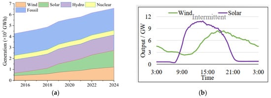
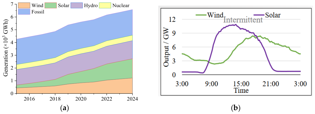
The global energy structure has undergone a historic transformation, with the proportion of sustainable energy rising. There has been a rise of intermittent energy such as wind and solar and intensifying grid fluctuations. This trend drives higher demand for flexible regulation in modern power systems, as shown in Figure 1. With its compact design and high efficiency, the Francis turbine plays a key role in grid-scale peak shaving.

Figure 1. Trends and intermittency of wind and solar power generation ((a) installed capacity trends over the past decade, (b) intermittency characteristics of wind and solar output over a 24-h period).

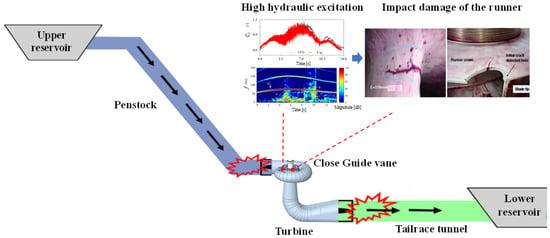
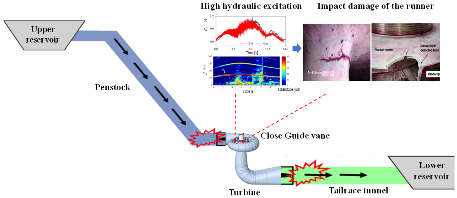
During grid regulation, turbines often experience sudden disconnection from the power grid due to protective trips or dispatch commands, entering a load rejection transient [1]. In this process, the turbine undergoes abrupt loss of load, prompting the governor to respond rapidly and drive the guide vane toward closure [2]. The turbine speed typically rises to runaway speed within 10 s, while the flow rate approaches zero within 20 s. The runner flow field sharply departs from design conditions, generating intense vortices and pressure pulsations that excite strong mechanical vibrations [3]. These complex hydraulic excitations amplify alternating blade loads, causing local stress concentrations that can initiate fatigue cracks and ultimately lead to structural failure, threatening unit safety and service life [4,5,6], as shown in Figure 2. Understanding runner fatigue under such transients is therefore critical.

Figure 2. Intense hydraulic excitation and impact damage during load rejection.

Scholars worldwide have extensively studied the complex flow mechanisms and hydraulic excitation during transient processes such as load rejection using experimental and numerical methods. Zhang et al. [7] investigated pressure pulsations in the draft tube and the dynamic evolution of vortex ropes during the runaway of a Francis turbine, showing that as conditions depart from the rated point, broken vortex ropes gradually merge into an eccentric rope. Fu et al. [8] applied dynamic mesh simulations to examine hydraulic instability under load rejection, revealing that vortices in double-row guide vanes induce the observed dynamic instability. Trivedi et al. [9] measured instantaneous pressure pulsations in a high-head Francis turbine model and found maximum amplitudes during runaway, which can directly impact turbine service life. Zeng et al. [10] analyzed the effect of guide vane closing laws on S-region transients and load rejection parameters in a pump turbine, providing insights for optimizing active guide vane control. Sun et al. [11] conducted numerical simulations using structured overlapping meshes and found that guide vane movements generate high-amplitude pressure pulsations and enlarge recirculation zones in the draft tube. Overall, vortex evolution during transient events intensifies hydraulic excitation, increasing the risk of unit instability and runner fatigue damage.

Surveys indicate that runners in many hydropower stations have developed cracks of varying degrees. To investigate the causes and dynamic characteristics of runner fatigue, scholars have primarily employed fluid–structure interaction (FSI) methods to perform structural and fatigue analyses on hydraulic machinery. Luna-Ramírez et al. [12] analyzed a 200 MW Francis turbine runner using CFD and finite element methods, identifying significant stress concentration at the T-joint between the blades and crown, explaining crack formation in this region. Saeed et al. [13] combined numerical simulation and stress finite element analysis to study runner blade cracks, finding high-stress areas at the trailing edge. Zhu et al. [14] experimentally determined that hydraulic instability under low-head, high-load, and small-opening conditions causes stress concentration at the trailing edge where blades connect with the crown and band, attributing cracks to combined static stress, hydraulic excitation, and residual stress. Xiao et al. [15] suggested that dynamic stress from non-design water pressure is a primary cause of fatigue and cracking. Liu et al. and Magnoli et al. [16,17] studied flow-induced stresses under three typical load conditions, confirming that high stresses from unsteady flow drive fatigue fractures. Li et al. [18] used a fatigue crack growth model with FSI to link runner blade ultimate strength to both vibration and fatigue characteristics. Wang et al. [19] numerically obtained stress distributions and studied runner stiffness, strength, and fatigue life, validating design optimization based on fatigue analysis. Zhang [20] numerically investigated the dynamic response of cracked Francis turbine runners, showing that increasing crack length alters dynamic characteristics, explained via crack vibration localization theory. Gagnon et al. [21] decomposed runner loading into LCF and HCF components, with only the LCF component contributing to initial crack propagation. In summary, stress concentrations are primarily located at T-joints between the blade trailing edge, crown, and band, with fatigue cracks mostly induced by high-amplitude dynamic stresses from hydraulic excitation.

Current studies lack a systematic analysis of runner fatigue characteristics under load rejection transients, particularly regarding the linkage between vortex structure evolution and the spatiotemporal variation of blade stress throughout the entire load rejection process. Moreover, existing fatigue assessments are mostly conducted on defect-free structures or only qualitatively identify critical stress locations, with limited quantitative damage evaluation for runners containing pre-existing cracks under transient loads.

This study aims to systematically investigate the internal flow evolution and transient hydraulic excitation characteristics of a Francis turbine during load rejection transients using CFD simulations coupled with one-way FSI methods. Particular emphasis is placed on examining the spatiotemporal correlation between vortex structure evolution and dynamic stress response of the runner blades under complex hydraulic loading, as well as identifying critical stress regions. Furthermore, by incorporating a pre-existing through-crack model into the transient FSI analysis and integrating a modified S-N curve with fatigue damage theory, a quantitative methodology for assessing runner fatigue damage under transient operating conditions is proposed. Specifically, the effects of initial defects on stress amplitude, mean stress, and standard deviation at critical locations are quantitatively compared. The cumulative fatigue damage of cracked runners under a single load rejection event is evaluated using the rain-flow counting method and the Palmgren–Miner rule, with particular attention to the sensitivity of fatigue damage to different residual stress levels (100, 150, and 200 MPa). The outcomes are expected to provide theoretical support for the structural design and operational maintenance of turbine runners.

2. Objective and Methodology

2.1. Research Objective

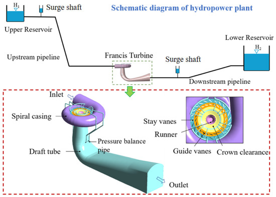
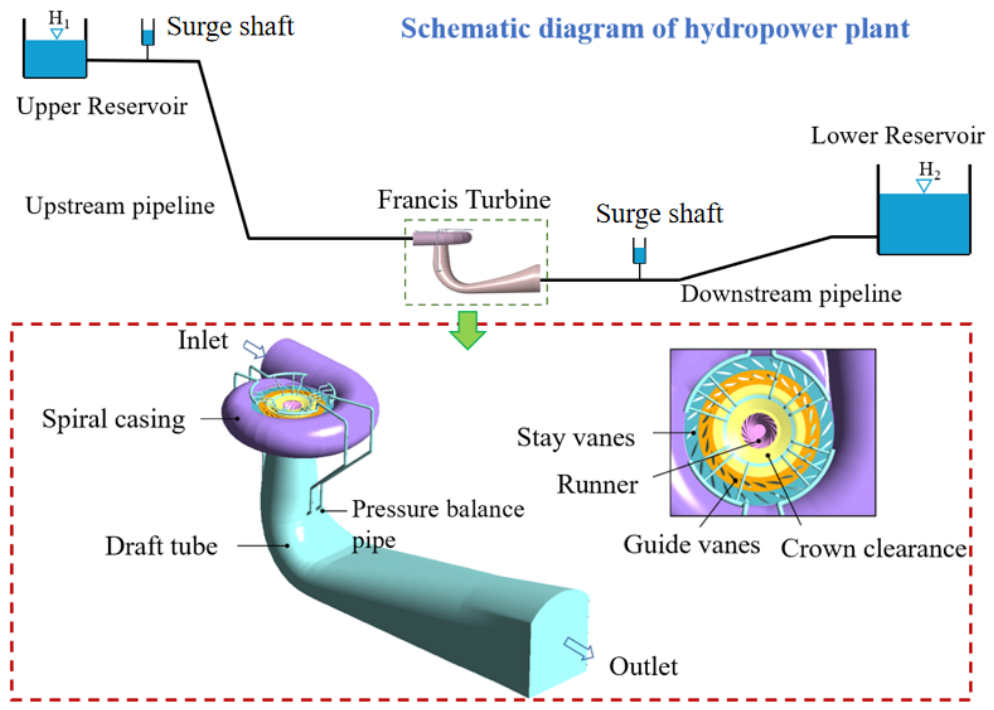
This study focuses on a Francis turbine in actual operation at a hydropower plant, with its key design parameters listed in Table 1. A 3D hydraulic model covering the entire flow passage (Figure 3) is developed using the software Creo 11.0. The model includes all flow components, such as the water conveyance system, spiral casing, stay vanes, guide vanes, runner, draft tube, pressure balance pipe, crown, and band, fully reproducing the actual flow passage geometry of the turbine.

Table 1. Main parameters of Francis turbine.

Condition	Description
Load rejection process	The turbine may suddenly disconnect from the power grid and lose all of its load due to system faults, entering a load rejection transient. The guide vane system responds rapidly to limit the rapid increase in runner speed.
Parameter	Value	Unit
Rated rotational speed, nr	125	r/min
Stay vanes number, Zs	23	[-]
Guide vanes number, Zg	24	[-]
Runner blade number, Zr	15	[-]

Figure 3. Hydropower plant model with water conveyance system and turbine.

2.2. Mesh Generation

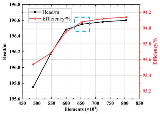
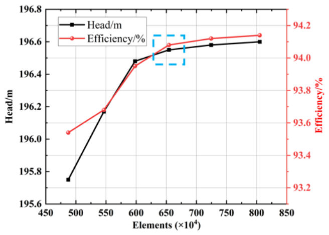
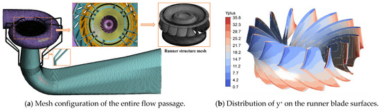
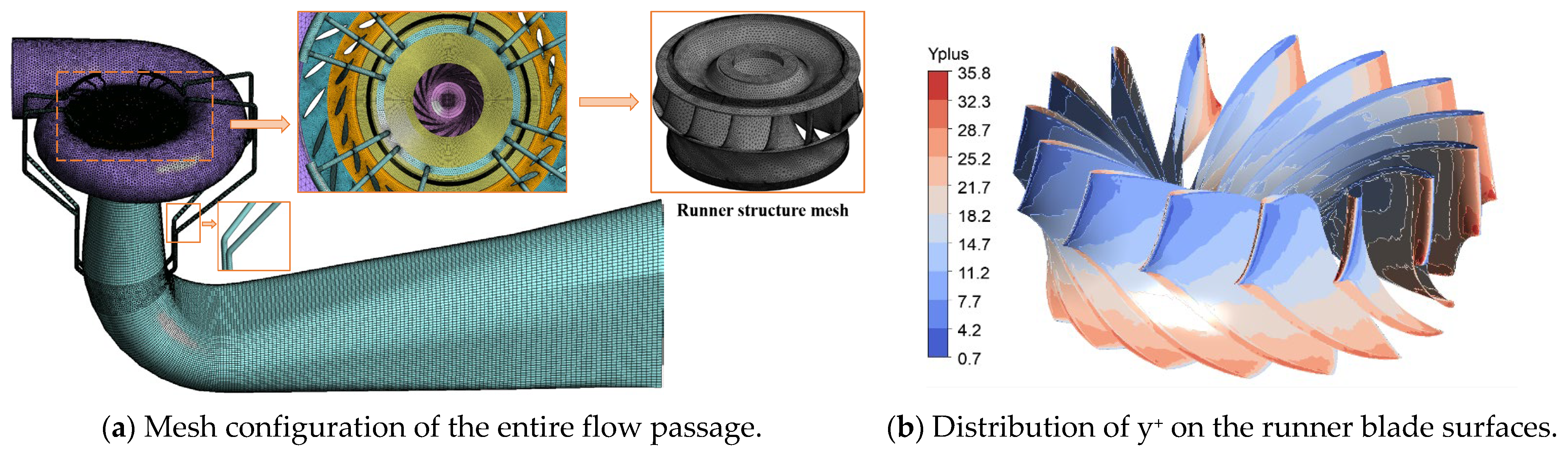
The fluid domains of the Francis turbine components are meshed using different strategies. Tetrahedral meshes with strong geometric adaptability are applied to the spiral case and runner, while structured hexahedral meshes are adopted for the remaining components [22]. To accurately capture viscous effects and steep velocity gradients near solid walls, multiple boundary-layer meshes are generated along the runner blades, with additional local refinement at the leading and trailing edges [23]. To assess mesh independence, six mesh schemes ranging from 4.87 million to 8.05 million cells are evaluated under rated head conditions. As shown in Figure 4, both unit head and efficiency generally increase with mesh number increase. Pronounced variations are observed when the mesh number was below 6.54 million, whereas the results gradually stabilize beyond this threshold. Balancing computational accuracy and efficiency, the fourth mesh scheme, consisting of 6,544,103 cells, is selected for subsequent simulations. The final mesh configuration is illustrated in Figure 5a. In addition, the near-wall mesh resolution was further assessed by examining the dimensionless wall distance y⁺ on the runner blade surfaces. The runner blades are the most geometrically complex components in the entire flow passage, featuring the highest curvature and thus imposing the most stringent requirements on boundary-layer meshing. Moreover, since the runner is the key component for the subsequent FSI-based stress and fatigue analysis, the y⁺ distribution on the blade surfaces is adopted as the primary indicator of near-wall mesh quality, as shown in Figure 5b. The vast majority of the blade surface exhibits low y⁺ values, with local peaks occurring only in very limited regions near the trailing edges. These local peaks are appropriately handled by the automatic wall treatment of the SST k-ω model. Therefore, the near-wall mesh resolution for the runner is considered adequate for the present study.

Figure 4. Grid independence verification.

Figure 5. Mesh generation of Francis turbine.

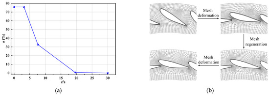
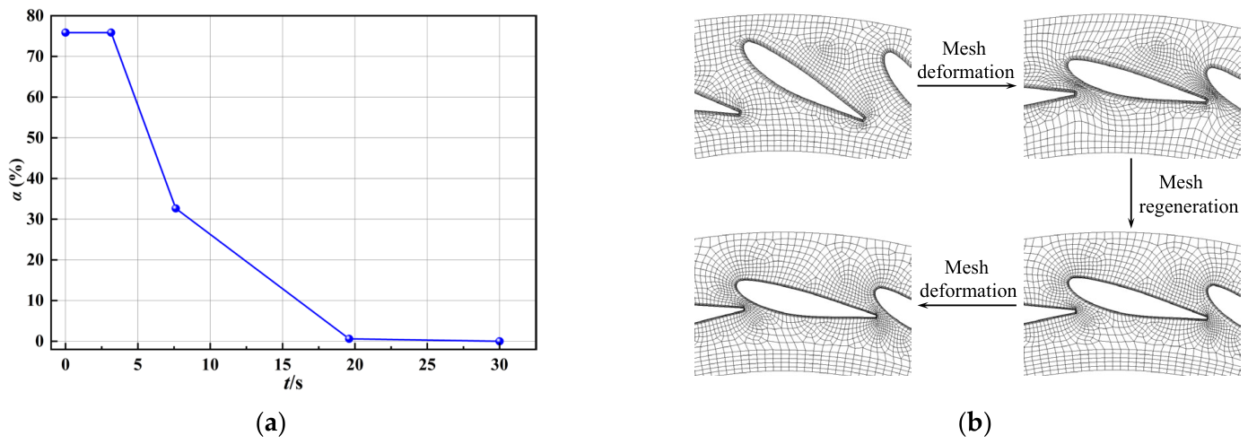
Based on the load rejection experimental data from the power station, this study adopts a two-stage guide vane closing strategy characterized by a “fast-then-slow” pattern, as illustrated in Figure 6a. During the dynamic mesh simulation, mesh updating is achieved in CFX-Pre by prescribing node displacements. To address local mesh deformation induced by guide vane motion, the Scripting language is used to call the Mesh module in ANSYS Mesh 14.5 module to regenerate the mesh of the guide vanes. Throughout the load rejection simulation, the guide vane domain is discretized using structured meshes with boundary layers, and the mesh quality is maintained at a high level during the entire closing process, as shown in Figure 6b.

Figure 6. Dynamic mesh setting during load rejection process ((a) guide vane closure law during the load rejection; (b) implementation of the dynamic mesh methodology).

2.3. Numerical Methods and Damage Modeling

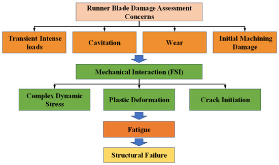
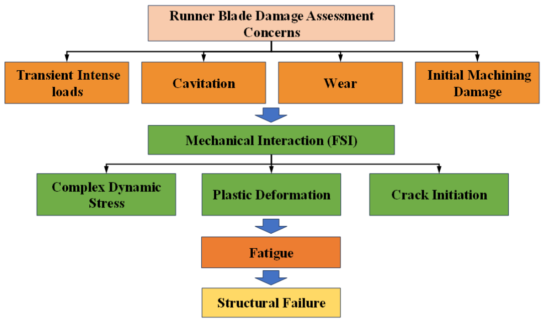
This study investigates the structural response and damage behavior of turbine runner blades subjected to strong hydraulic excitation during the load rejection process. Emphasis is placed on plastic deformation-dominated failure driven by transient hydraulic loads, while the coupled effects of multiple damage mechanisms, including wear, corrosion, impact damage, cavitation, and manufacturing defects, are also considered. These damage modes may interact and significantly accelerate blade degradation under extreme operating conditions. From an integrated perspective, the main blade failure modes under transient hydraulic excitation are first summarized. Subsequently, the influence of pre-existing damage on blade fatigue life is examined, and the necessity of introducing initial damage states in fatigue assessment is discussed. The research approach is shown in Figure 7.

Figure 7. Key concerns affecting turbine runner blades leading to structural degradation.

2.3.1. Turbulence Model and Numerical Scheme

ANSYS CFX 2023 R2 is used to conduct CFD simulations of the Francis turbine. The SST k-ω turbulence model is adopted to close the Reynolds-averaged Navier–Stokes equations, combining the advantages of the k-ε model in the core flow region with those of the k-ω model in the near-wall region (Equations (1) and (2)) [24]. Given that the present study focuses on the relatively extreme load rejection transient, the SST k-ω turbulence model is employed to achieve a favorable balance between computational cost and numerical robustness, thereby ensuring the reliability of the subsequent stress analysis. To account for the weak compressibility of the fluid under the water hammer effect in transient conditions, the weakly compressible fluid model (Equations (3) and (4)) is employed in this study for accurate characterization of the dynamic response [25]. The rotor–stator interaction between the rotating and stationary components (i.e., runner, guide vanes, and draft tube) is modeled using the Frozen Rotor approach for steady-state simulations and the Transient Rotor-Stator interface for unsteady simulations. The high-resolution advection scheme and second-order backward Euler scheme are applied for spatial and temporal discretization, respectively. For the transient simulations, the time step is set to Δt = 60/(n × 180) = 0.002667 s, and the maximum number of iterations per time step is set to 20.

$${\displaystyle \frac{\partial \left(\rho k\right)}{\partial t}}+{\displaystyle \frac{\partial }{\partial x_j}}\left(\rho U_{j}k\right)-{\displaystyle \frac{\partial }{\partial x_j}}\left[\left(\mu +{\sigma }_k{\mu }_t\right){\displaystyle \frac{\partial k}{\partial x_j}}\right]=P_k-{\beta }^{\prime }\rho k\omega$$

(1)

$${\displaystyle \frac{\partial }{\partial t}}\left(\rho \omega \right)+{\displaystyle \frac{\partial }{\partial x_j}}\left(\rho U_j\omega \right)=C_{\omega }{P}_k-\beta \rho {\omega }^2+{\displaystyle \frac{\partial }{\partial x_j}}\left[\left(\mu +{\sigma }_{\omega }{\mu }_t\right){\displaystyle \frac{\partial \omega }{\partial x_j}}\right]+2\left(1-F_1\right){\displaystyle \frac{\rho {\sigma }_{\omega 2}}{\omega }}{\displaystyle \frac{\partial k}{\partial x_j}}{\displaystyle \frac{\partial \omega }{\partial x_j}}$$

(2)

$$\rho ={\displaystyle \frac{{\rho }_0}{1-\frac{P}{K}}}$$

(3)

$${\displaystyle \frac{\partial \left({\rho }_m{u}_i\right)}{\partial t}}+{\displaystyle \frac{\partial \left({\rho }_m{u}_i{u}_j\right)}{\partial x_j}}=-{\displaystyle \frac{\partial }{\partial x_i}}[p+{\displaystyle \frac{2}{3}}{\mu }_m{\displaystyle \frac{\partial u_j}{\partial x_j}}]+{\displaystyle \frac{\partial ({\mu }_m+{\mu }_t)}{\partial x_i}}({\displaystyle \frac{\partial u_i}{\partial x_j}}+{\displaystyle \frac{\partial u_j}{\partial x_i}})+{\rho }_m{g}_i$$

(4)

where k is the turbulent kinetic energy, x_j is the spatial coordinate, P_k is the turbulence production term, μ is the dynamic viscosity, ω stands for the specific dissipation rate, μ_t signifies the turbulent eddy viscosity, C_ω is the production coefficient, F₁ serves as the blending function, σ_ω, β, and σ_ω2 constitute the closure coefficients, ρ is the water density, ρ₀ is the reference density of 998.2 kg/m³, P denotes the gauge pressure of water, and K is the bulk modulus of water.

During the load rejection process, the sudden change in external load causes torque imbalance in the rotor system, and the action of hydraulic torque drives a rapid increase in rotational speed. To accurately simulate this transient dynamic response, this study establishes a finite-difference solution scheme based on the conservation law of angular momentum (Equations (5) and (6)) and implements dynamic iterative calculation of rotational speed at each time step using a Fortran program, thereby ensuring the physical accuracy of rotational speed evolution and operational state prediction during the load rejection process.

$${\omega }_{i+1}={\omega }_i+{\displaystyle \frac{M_i}{J_z}}∆t$$

(5)

$$J_z={\displaystyle \frac{1}{4}}G{D}^2$$

(6)

where ω is the angular velocity of the runner, $M_i$ is the hydraulic torque on the runner, $J_z$ is the moment of inertia of the rotor system, Δt is the numerical simulation time step.

2.3.2. FSI Simulation Model

Once the hydraulic excitation is obtained, the pressure pulsations acting on the blade surfaces are transferred to the finite element model (FEM) to evaluate the static and dynamic stress responses. A fluid–structure interaction (FSI) analysis framework based on CFX and Transient Structural is established, in which a one-to-one nodal correspondence between the CFD and FEM meshes on the blade surfaces ensures accurate pressure transfer at each time step [26]. During operation, the blades are simultaneously subjected to hydraulic excitation and centrifugal loads. The induced structural vibrations and elastic deformations further disturb the surrounding flow field. Therefore, the runner dynamic response must be treated as a one-way coupled fluid–structure interaction problem. The solid momentum equation is derived from Newton’s second law (Equation (7)). At the fluid–structure interface, continuity conditions ensure momentum and energy conservation (Equation (8)). The runner dynamic stress is obtained by solving the structural equilibrium equation (Equation (9)), and the equivalent stress is evaluated using the fourth strength theory (Equation (10)).

$${\rho }_s\ddot{d_s}=\nabla ·{\sigma }_s+f_s$$

(7)

$$\left\{\begin{array}{c}{\tau }_f·n_f={\tau }_s·n_s\\ d_f=d_s\\ q_f=q_s\\ T_f=T_s\end{array}\right.$$

(8)

$$\left[M\right]\left\{\ddot{u}\right\}+\left[C\right]\left\{\dot{u}\right\}+\left[K\right]\left\{u\right\}=\left\{F\right\}$$

(9)

$$\sigma =\sqrt{{\displaystyle \frac{1}{2}}\left[{\left({\sigma }_1-{\sigma }_2\right)}^2+{\left({\sigma }_2-{\sigma }_3\right)}^2+{\left({\sigma }_3-{\sigma }_1\right)}^2\right]+6({\tau }_{12}^2+{\tau }_{23}^2+{\tau }_{31}^2)}$$

(10)

where ρ_s is the solid density, $\ddot{d_s}$ is the solid acceleration vector, ${\sigma }_s$ is the Cauchy stress tensor, and f_s accounts for the external forces, n is the interface normal vector, τ is the stress tensor, d represents the displacement vector, q is the heat flux, and T is the temperature; ([M]), ([C]), and ([K]) are the mass, damping, and stiffness matrices; {$u$},{$\dot{u}$},{$\ddot{u}$} are nodal displacement, velocity, and acceleration vectors; {F} is the nodal load vector due to gravity, centrifugal force, and hydraulic pressure, ${\sigma }_1$, ${\sigma }_2$, ${\sigma }_3$ and ${\tau }_{12}$, ${\tau }_{23},$ and ${\tau }_{31}$ are normal and shear stresses in the (x), (y), and (z) directions.

2.3.3. Structural Damage Assessment Model

In structural fatigue life prediction, the S-N curve is a fundamental model for characterizing the fatigue behavior of materials [27,28]. The power-law S-N relationship proposed by Basquin and its logarithmic form reveal a linear relationship between stress amplitude and fatigue life in logarithmic coordinates:

$${\sigma }^{m}N=C$$

(11)

$$lgN=a+blsS$$

(12)

where N is the number of cycles at a certain stress level, m and C are material constants, S is the stress level, a and b are undetermined coefficients in the expression.

The fatigue tested of the runner material ZG0Cr13Ni4Mo in water was conducted in reference [29], obtaining the S-N expression for 99% survival rate in water.

$$lgN=18.2506-5.05lgS$$

(13)

In practical engineering fatigue assessments, the theoretical S-N curve must be modified to account for multiple influencing factors. In this study, fatigue life is evaluated based on the maximum stress at critical locations; therefore, the local stress concentration factor K_f is not introduced. Considering that a Francis turbine runner is a large, welded structure, the main correction factors include:

(a)

Size effect factor ε: According to Ref. [30], ε = 0.7 is adopted to account for the influence of component size on fatigue strength.

(b)

Surface finish factor β: Referring to ASME and IEC standards, a conservative value of β = 0.65 is used for welded surfaces.

(c)

Welding residual stress σ_res: Based on Ref. [31], a residual tensile stress of 250 MPa is assumed and incorporated into the mean stress correction as an additional mean stress component.

Through the above analysis, combined with the Goodman mean stress correction, the corrected equivalent nominal stress expression was obtained as follows:

$${\sigma }_{-1}={\displaystyle \frac{{\sigma }_b·{\sigma }_a}{\epsilon ·\beta ·\left[{\sigma }_b-\left({\sigma }_m+{\sigma }_{res}\right)\right]}}$$

(14)

By substituting Equation (14) into the material S-N relationship given in Equation (15), a corrected S-N curve applicable to the actual runner structure is obtained and subsequently used for fatigue life prediction.

$$lgN=18.2506-5.05lg{\displaystyle \frac{1758.2417·{\sigma }_a}{550-{\sigma }_m}}$$

(15)

2.4. Experimental Validation

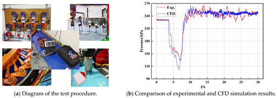
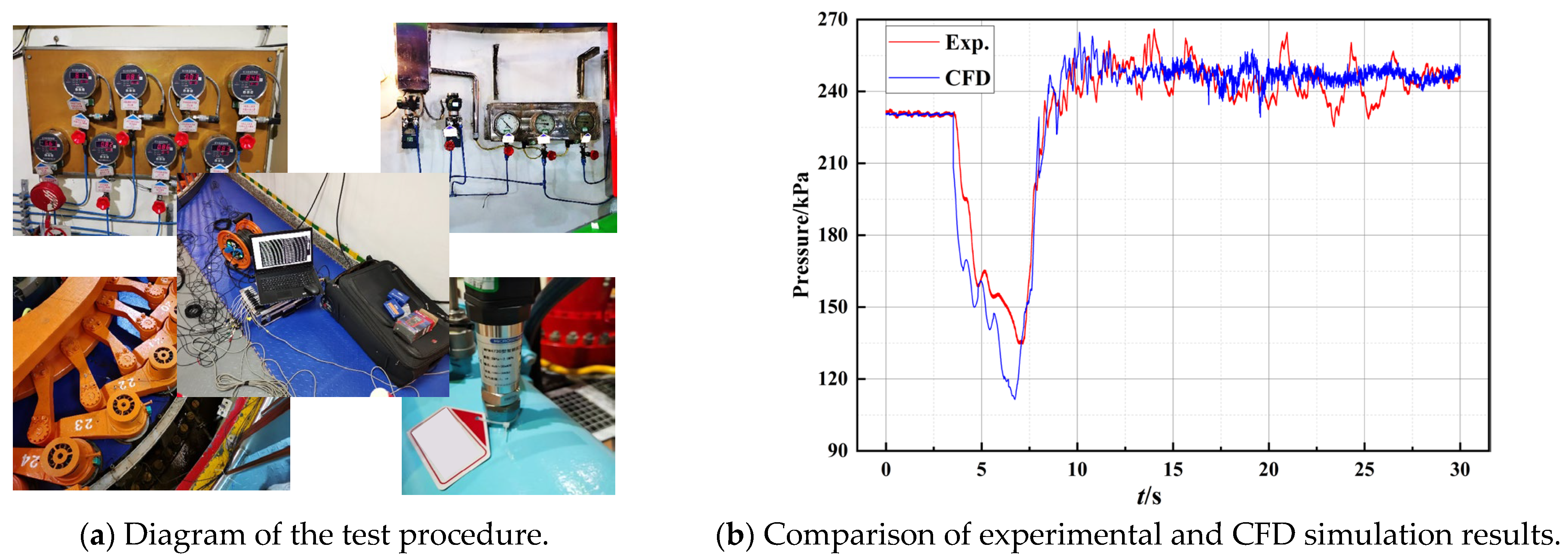
To verify the accuracy of the numerical simulation for the load rejection transient process, Figure 8 presents a comparison between experimental and simulated results for the pressure monitoring point at 0.3 D in the straight conical section of the draft tube. Although discrepancies exist between the simulated pressure values and the experimental data at this location, the overall temporal trends show good agreement. Direct strain validation is not included due to the absence of on-site strain-gauge data during the transient. At 7 s, the discrepancy between the experimental and simulated values reaches its maximum, approximately 28.8%. Beyond this point, the deviation between the experimental and simulated results decreases significantly and becomes almost negligible. After 10 s, the maximum error is reduced to 7%. The results indicate that the adopted numerical approach can effectively capture the dynamic flow characteristics during load rejection, providing a reliable basis for subsequent analysis of unit transient external characteristics and the application of fluid–structure interaction loads.

Figure 8. Comparison of draft pressure between simulation and experiment during load rejection process.

3. Results and Discussion

3.1. Analysis of Hydraulic Characteristics and Internal Flow Evolution During Load Rejection Process

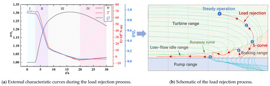
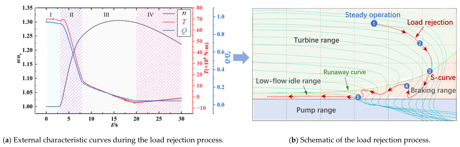
Figure 9 presents the dimensionless normalized rotational speed (n), flow rate (Q), and torque (T) of a Francis turbine during the load rejection process. According to the guide vane closing law, the entire load rejection transient process was divided into four stages: I, II, III, and IV. In Stage I (0–3.15 s), the unit remains in a rated steady-state condition prior to load rejection, with both guide vane opening and rotational speed maintained at constant levels. In Stage II (3.15–7.62 s), the rapid closure of guide vanes results in a sharp decrease in flow rate and driving torque, while the residual energy of the unit after grid disconnection leads to a rapid rise in rotational speed. In Stage III (7.62–19.6 s), the reduced closure rate of guide vanes leads to a continued decline in flow and torque, with torque reversing to negative values around 15.5 s. The combined effect of diminishing flow and negative torque generation causes the rotational speed to peak at 15.5 s before initiating a decrease. In Stage IV (19.6–30 s), the guide vanes approach complete closure, flow stabilizes at a low level, reverse torque exhibits a gradual attenuation, and rotational speed continues to decline. During the load rejection process, the turbine transitions from the rated condition through the acceleration range and the reverse braking range to the low-flow idling range, accompanied by a rapid rise in rotational speed, torque reversal, and flow instability.

Figure 9. Rotational speed, torque, and flow rate during load rejection.

To study the transient flow mechanism during the load rejection process, six typical moments were selected for analysis, and the main parameters of each moment are shown in Table 2. Among them, t₁ = 3.5 s is the rated condition before load rejection, t₂ = 6.2 s is the key moment of the fast-closing stage of the guide vanes, t₃ = 7.6 s is the switching point of the guide vane closing law, t₄ = 9.7 s is the key moment of the slow-closing stage of the guide vanes, t₅ = 15.5 s is the moment of maximum speed, and t₆ = 19.6 s indicates the instant when the guide vanes are essentially fully closed.

Table 2. Main parameters of typical moments during load rejection.

Time/s	GVO/°	Q/Qr	n/nr	H/Hr
t1 = 3.5	23.34	0.911	1.022	1.095
t2 = 6.2	14.29	0.528	1.2	1.249
t3 = 7.6	9.2	0.299	1.243	1.222
t4 = 9.7	7.58	0.194	1.278	1.078
t5 = 15.5	5.3	0.1	1.305	1.069
t6 = 19.6	4.08	0.048	1.298	1.08

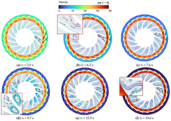
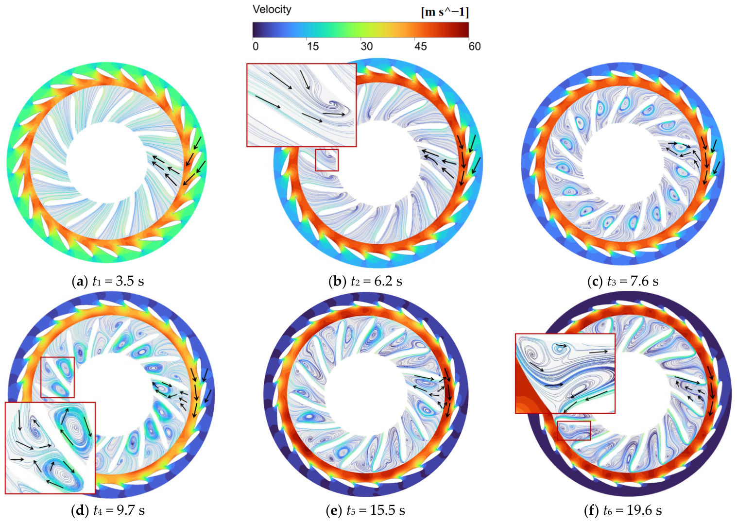
The complex dynamic evolution of the flow field during the load rejection process is the fundamental cause of hydraulic excitation loads [32]. Figure 10 presents the velocity and streamline distributions at six representative instants during the load rejection process.

Figure 10. Velocity distribution of guide vanes and runner at representative instants.

At t₁ = 3.5 s, the unit operates under rated condition prior to load rejection, with smooth and uniformly distributed streamlines in the flow passage and no significant flow separation or vortex structures observed. At t₂ = 6.2 s, the guide vanes are in a rapid closing stage, leading to a pronounced velocity gradient within the flow passages. The velocity in the vaneless region increased markedly, while the inlet velocity of the guide vanes begins to decrease. An incipient low-speed vortex is observed near the trailing edge on the pressure side of the runner blades. By t₃ = 7.6 s, the guide vane inlet velocity further declines and the runner flow field deteriorates, giving rise to a distinct double-vortex structure within each blade passage. A small-scale vortex forms near the pressure-side leading edge, whereas a large single-peaked elliptical vortex, biases toward the suction side, occupied the mid-passage. At t₄ = 9.7 s, the double-vortex structure expands to fill the entire runner passage, while the velocity in the vaneless region weakened. During t₅ = 15.5 s and t₆ =19.6 s, the guide vane inlet velocity approached zero, the residual high-speed flow is confined to the vaneless region, the original double-vortex structure fragment into irregular vortical clusters of various scales, and reverse flow developed along the suction surfaces of the runner blades.

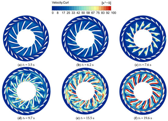
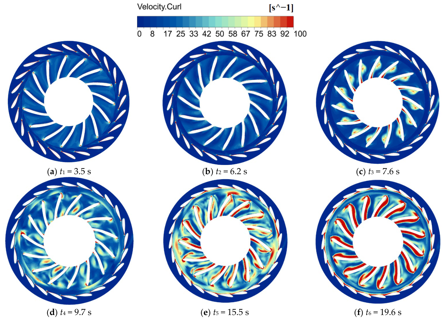
Figure 11 presents the vorticity distributions on the mid-span sections of the guide vanes and the runner. At t₁ = 3.5 s and t₂ = 6.2 s, the flow remains relatively stable and no distinct vortex cores are observed. By t₃ = 7.6 s, elongated vortices appear near the trailing edge on the suction side of the runner blades, while concentrated vortex regions develop in the center of the runner passages, corresponding to the regular double-vortex structure shown in Figure 10. At t₄ = 9.7 s, this regularity is disrupted and numerous discrete vortical structures emerge within the runner passages. Meanwhile, elongated vortex arcs form in the vaneless space and exhibit a tendency to merge. At t₅ = 15.5 s, the vorticity level increases sharply throughout the runner, with vortical structures occupying almost the entire flow passage and high-intensity vortices forming near the blade suction surfaces. In the vaneless region, pronounced velocity gradients between the runner and the guide vanes, together with outlet backflow, generate annular vortex systems that impinge on the pressure sides of the guide vanes. At t₆ = 19.6 s, periodic high-vorticity bands develop along the blade suction surfaces, corresponding to the stable reverse-flow region identified in Figure 10.

Figure 11. Mid-span vorticity distributions at representative instants of guide vane and runner.

The irregular vortex clusters directly alter the pressure distribution on the blade surfaces, leading to the generation of strong unsteady hydraulic loads. The various stages of vortex evolution—generation, development, and breakdown—correspond to distinct pressure fluctuation patterns.

3.2. Dynamic Blade Load During Load Rejection

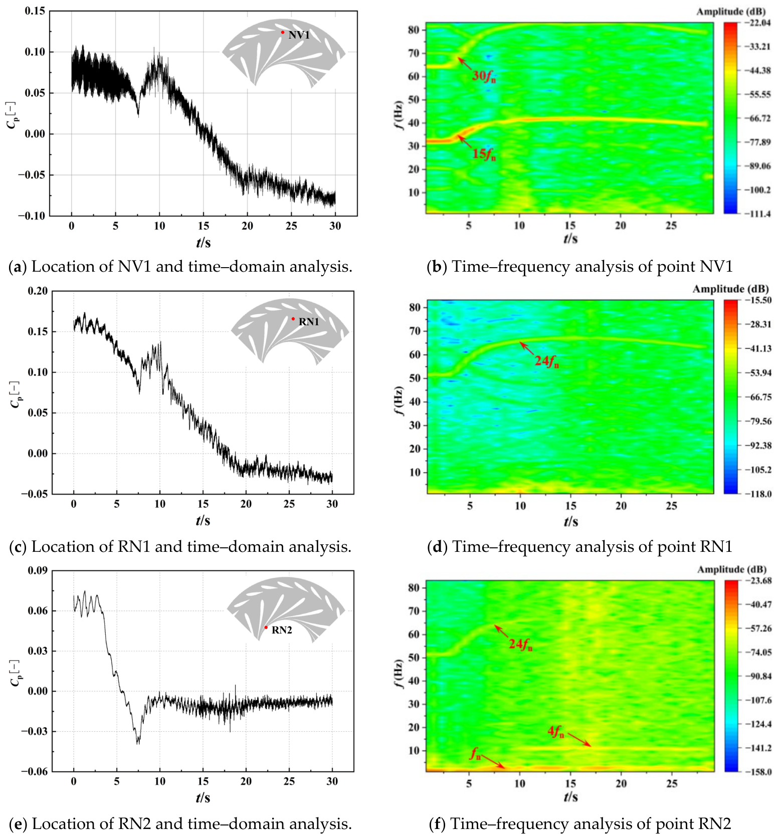
During the load rejection process, the internal flow state within the turbine undergoes intense variation, resulting in significant alterations to the amplitude and frequency of pressure pulsations in the unit. To investigate the fatigue mechanism of the runner, it is necessary to acquire the local dynamic stress–strain time history determined by the hydraulic excitation of the flow field. Therefore, emphasis is placed on analyzing the pressure pulsation load characteristics during the transient process. Monitoring points RN1 and RN2 are positioned at the runner inlet and outlet, respectively, while NV1 is located in the vaneless region [33,34]. The dimensionless coefficient Cp was introduced to quantify the intensity of pressure pulsation, as defined in Equation (16). Subsequently, the dimensionless pressure pulsation signals in the time domain were analyzed using short-time Fourier transform (STFT) to extract characteristic frequencies and track their temporal evolution in amplitude.

$$C_p={\displaystyle \frac{p-\overline{p}}{\rho gH}}$$

(16)

where $p$ is the instantaneous pressure at the monitoring point, $\overline{p}$ is the average pressure over the calculation cycle, $\rho$ is the density of the fluid, $g$ is the acceleration due to gravity, and $H$ is the head.

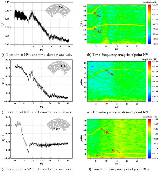
Figure 12 presents the time-domain evolution of the pressure coefficient C_p at the main monitoring points during the load rejection process. The results indicate an approximately linear variation in pressure. During the interval from t = 3.15 s to t = 7.62 s, rapid guide vane closure leads to a sharp pressure drop at all locations. At t = 7.62 s, when the guide vane closing law changes abruptly, the pressure signals display a transient increase followed by a subsequent decrease, with varying magnitudes among the monitoring points. By t = 19.6 s, when the guide vanes are nearly fully closed, the pressure decay at monitoring points NV1 and RN1 becomes less pronounced, whereas a slight pressure rise is observed at the runner outlet monitoring point RN2. Frequency–domain analysis of the pressure pulsations reveals dominant low-frequency components in the range of 0–3 Hz, corresponding to the runner rotational frequency. The spectrum at the vaneless region monitoring point NV1 exhibits two distinct frequency bands associated with the runner blade-passing frequency 15f_n and its second harmonic 30f_n, with the former showing a higher amplitude. These features arise from rotor–stator interaction. Furthermore, owing to changes in the guide-vane closing law, enhanced low-frequency components in the range of 0–10 Hz appear around t = 9.62 s. Both runner inlet and outlet monitoring points (RN1 and RN2) display the guide-vane passing frequency 24f_n, although the amplitude at RN1 is significantly higher than at RN2, reflecting the downstream attenuation of pressure pulsations. In addition, a slight variation in the low-frequency bandwidth is observed at RN1, while RN2 exhibits intermittent high-amplitude frequency bands near the instant of maximum rotational speed at t = 15.5 s.

Figure 12. Time–frequency analysis of pressure signals at monitoring points.

Due to the strong unsteady interaction between the guide vanes and the runner blades, the runner inlet monitoring point RN1 exhibits the highest pressure pulsation amplitude, reaching up to 17.5%. In the vaneless region (NV1), although the pressure amplitude (10.1%) is lower than that at RN1, the fluctuation frequency is substantially higher. At this location, the flow is dominated by rotor–stator interaction, with the blade-passing frequency (15f_n) becoming the most prominent spectral component and displaying high amplitude in the time-frequency distribution. At the runner outlet (RN2), the flow undergoes significant energy dissipation through the runner passages, leading to attenuated pressure fluctuations. The flow exiting the runner is characterized by low-frequency vortex rope oscillations rather than high-frequency rotor-stator interactions, which explains the predominance of low-frequency components and the minimum pressure pulsation amplitude in the time-frequency diagram (decreasing from 7.5% at the early stage to only 2% at the final stage).

Within the period of 0–3.5 s, the rotor–stator interaction in the vaneless region is prominent, with the highest amplitude occurring at the 15f_n frequency. During the rapid guide vane closure stage (3.5 s–7.6 s), the dominant frequencies shift toward higher values: in the vaneless region, the 30f_n frequency band drifts from 62.5 Hz to 80 Hz, and the 15f_n band drifts from 31.25 Hz to 40 Hz; within the runner, the 24f_n band drifts from 50 Hz to 65 Hz. During the slow closure stage (7.6 s–19.6 s), the drift gradually decelerates and exhibits a decreasing trend.

3.3. Dynamic Stress Evolution Characteristics in the Runner During Load Rejection

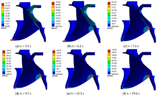
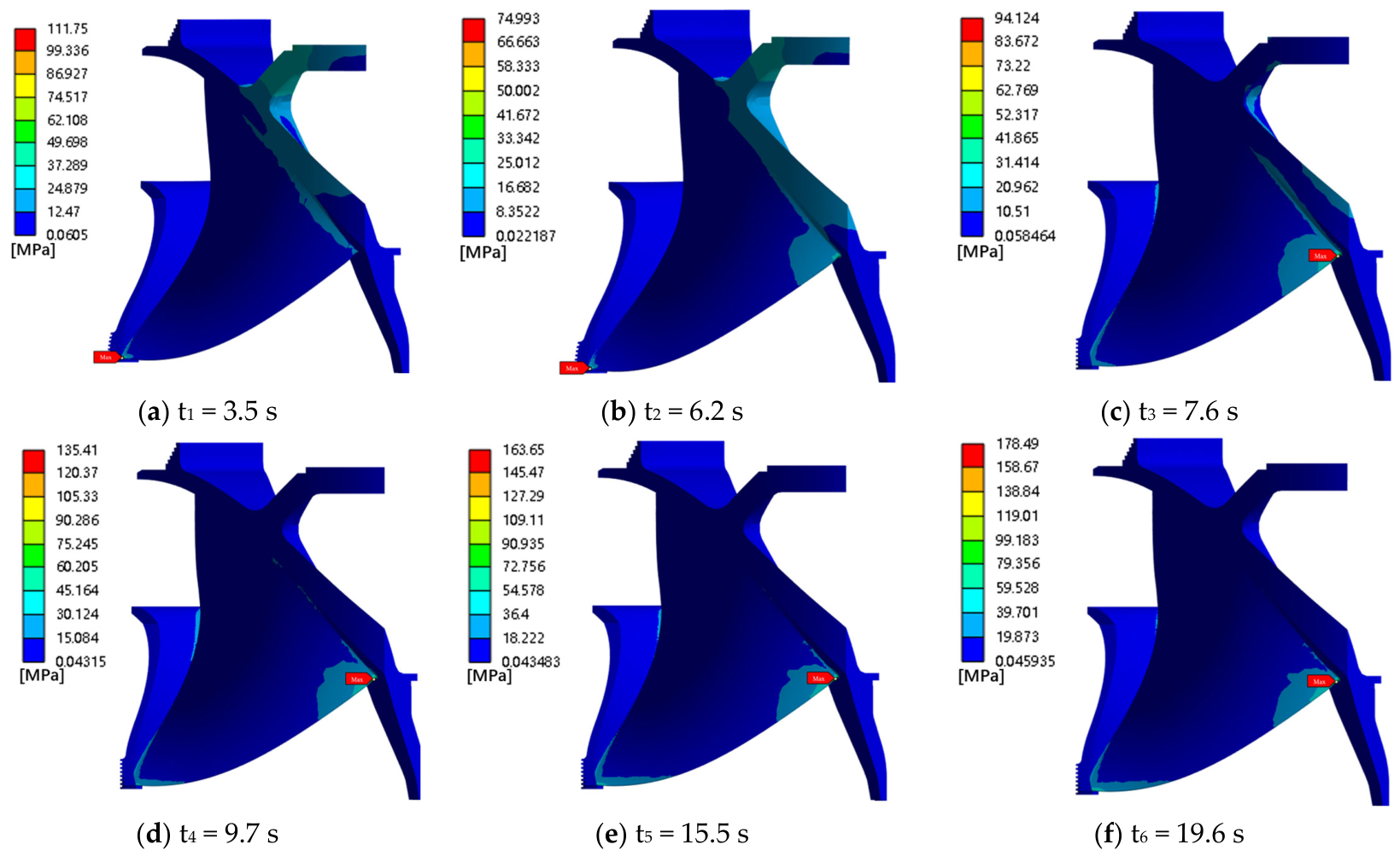
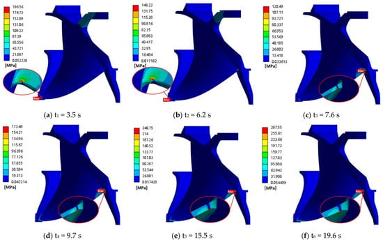
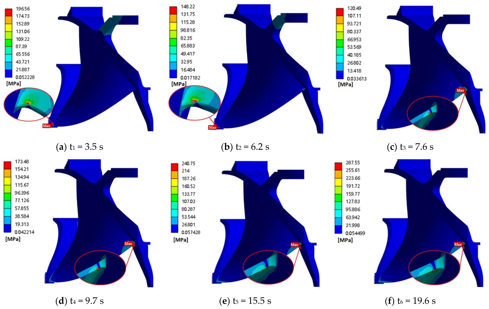
Through fluid–structure interaction, the hydraulic excitation loads during the load rejection process are applied to the blades to obtain the dynamic stress evolution of the runner. Figure 13 presents the equivalent stress distribution on the runner blades at distinct instants during the load rejection process. The red label in the figure indicates the location of the maximum equivalent stress. Overall, the maximum equivalent stress was distributed at the T-joint between the blade trailing edge and the crown or band. As the load rejection process progresses and the speed increased, the position of maximum equivalent stress gradually shifted from the connection with the band to the connection with the crown. In summary, during the load rejection process, the runner forms a complex stress state under the coupled action of centrifugal force and fluid pressure, with critical stress regions located at the T-joints between the blade trailing edge and the crown or band.

Figure 13. Equivalent stress distribution of runner at different moments during load rejection.

As Figure 13 shows, the maximum equivalent stress is 178.49 MPa, whereas under the cracked condition, it reaches 287.55 MPa, representing an increase of 61.1%. For the uncracked case, the maximum equivalent stress first decreases rapidly from 111.75 MPa at t₁ = 3.5 s to 74.99 MPa at t₂ = 6.2 s. This initial decrease is primarily attributed to the sharp reduction in flow rate and hydraulic loading on the blade surfaces caused by the rapid guide vane closure. Subsequently, the maximum equivalent stress gradually increases to its peak of 178.49 MPa at t₅ = 15.5 s. The increase from t₂ to t₅ is approximately 138%, and the overall increase from t₁ to t₅ is approximately 59.72%. The most pronounced stress rise occurs during the slow closure stage (from t₃ to t₅).

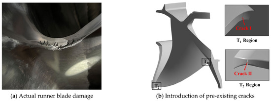
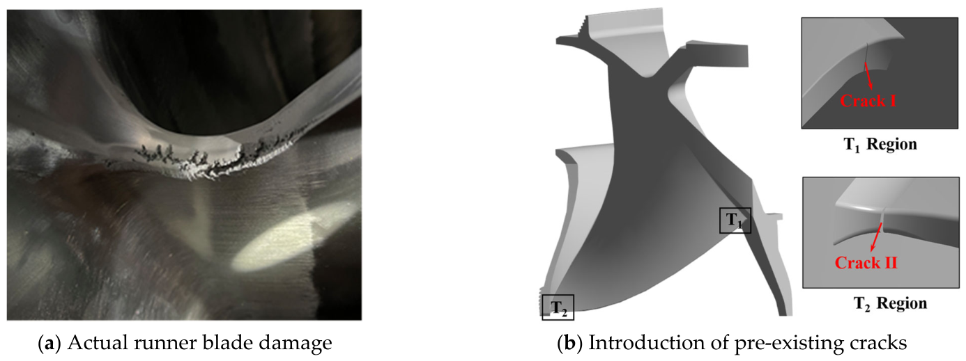
Wang et al. [35] demonstrated through correlation analysis between blade stress and fatigue life that regions with higher stress amplitudes are the first to undergo fatigue failure. In this study, potential damage at the T-joints, such as wear, cavitation, and manufacturing defects, is additionally considered. As shown in Figure 14a, an actual runner damage profile is presented, where the damaged area closely coincides with the stress concentration zone. Under the coupled effect of stress concentration and pre-existing damage, more pronounced stress concentration is generated at the crack tip and surrounding regions, thereby accelerating the fatigue or plastic failure of the runner. To simulate this condition, pre-existing through-cracks of 4 mm are introduced in the T₁ and T₂ regions of the blade trailing edge, as illustrated in Figure 14b. The pre-existing crack is modeled as a through-crack oriented perpendicular to the blade edge, with local mesh refinement applied in the vicinity of the crack tip. Considering manufacturing-induced defects and in-service wear, the crack length is defined as 4 mm. The evolution of dynamic stress during the load rejection process is then comparatively analyzed for both the undamaged and damaged configurations.

Figure 14. Actual runner blade damage photograph and introduction of pre-existing cracks in T₁ and T₂ of blade trailing edge.

Figure 15 presents the equivalent stress distribution on the runner blades with pre-existing cracks at distinct instants during the load rejection process. It can be observed that the presence of pre-existing cracks causes the relatively high-stress zones originally located in the crown region during load rejection to largely disappear, while pronounced equivalent-stress gradients emerge in the T₁ and T₂ regions of the blade trailing edge. Compared with the results in Figure 13, the introduction of pre-existing cracks does not alter the location of the maximum equivalent stress during the transient process. At instants t₁ and t₂, the maximum equivalent stress is located in the T₂ region, whereas from t₃ to t₆ it shifts to the T₁ region. However, at each corresponding instant, the magnitude of the maximum equivalent stress is notably higher in the presence of pre-existing cracks. These results indicate that crack introduction significantly intensifies stress concentration and modifies local stiffness, which in turn directly amplifies the alternating stress, thereby substantially reducing the fatigue life of the runner.

Figure 15. Equivalent stress distribution of cracked runner at different moments during load rejection.

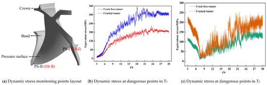
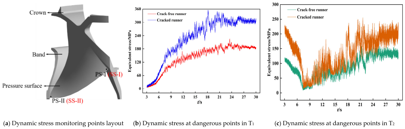
To further study the influence of pre-existing cracks on the dynamic stress at critical locations of the runner during load rejection, stress monitoring points were established in the T-type regions of the blade trailing edge, as illustrated in Figure 16a. The monitoring points located in the T₁ region are labeled as Point I, those in the T₂ region as Point II. The points on the intact (pre-crack-free) structure are denoted as PS, while those on the structure containing pre-existing cracks are denoted as SS. Figure 16b,c compare the dynamic stress responses at critical points with and without pre-existing cracks in the T₁ and T₂ regions throughout the load rejection transient. The results indicate that the pre-existing crack in T₁ had a negligible effect on the stress at the initial stage of load rejection. However, as the transient progressed, the influence of the crack on the equivalent stress gradually became more pronounced. In contrast, the pre-existing crack in T₂ exerted a considerable influence on the stress level even during the early phase. Before 6.7 s, the stress difference between cracked and uncracked configurations gradually diminished. Between 6.7 s and 9.7 s, the stress levels of the two cases remained largely comparable, after which the discrepancy in stress magnitude progressively increased. Throughout the load rejection process, the presence of a pre-existing crack in T₂ markedly amplified the stress fluctuation amplitude at the critical point. It can be concluded that the introduction of pre-existing cracks substantially elevates both the mean stress level and the stress amplitude during load rejection, thereby destabilizing the dynamic stress response and significantly accelerating fatigue damage in the runner. Moreover, at t = 7.6 s, the location of the maximum stress shifts from the band-side to the crown-side T-junction, corresponding to the abrupt changes in C_p at each monitoring point shown in Figure 12. Moreover, the stresses at the critical points (T₁ and T₂) continue to increase after 7.6 s with strong fluctuations.

Figure 16. Dynamic stress comparison at T₁/T₂ regions with/without pre-existing cracks during load rejection.

The evolution of vortex structures generates pressure pulsations with characteristic frequencies and amplitudes, which in turn impose time-varying loads on the runner blades, ultimately determining the spatiotemporal distribution of dynamic stresses.

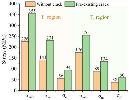
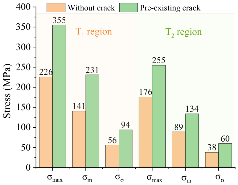
To quantify the influence of pre-existing cracks on the dynamic stress during load rejection, Figure 17 presents a statistical comparison of three parameters: maximum stress (σ_max), mean stress (σ_m), and standard deviation (σ_σ) at critical locations in the T₁ and T₂ regions, both with and without damage. The results indicate that pre-existing damages significantly increase all three parameters, demonstrating that their introduction substantially elevates the stress level and stress amplitude during the load rejection process, while also enhancing the instability of the dynamic stress response. Overall, although pre-existing cracks do not alter the location of the maximum equivalent stress, they comprehensively raise the stress level and amplitude at critical points, thereby degrading the fatigue performance of the runner, accelerating fatigue damage, and reducing its service life.

Figure 17. Comparison of stress of critical points with and without damage during load rejection.

3.4. Fatigue Life Assessment of Turbine Runners During Load Rejection Process

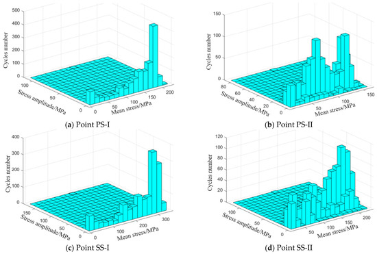
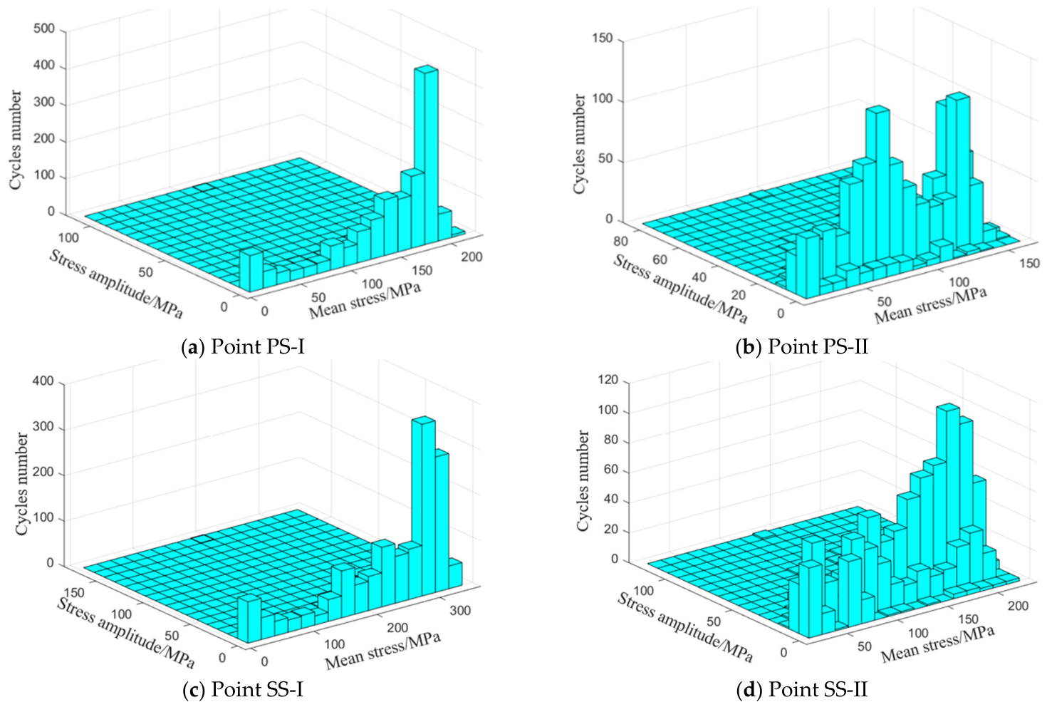
To achieve fatigue damage calculations for critical areas, the dynamic stress calculation results of the last three periods were used as the basis for analysis. The dynamic stress data of the four monitoring points of the runner with or without pre-existing cracks were subjected to rain–flow counting using MATLAB 9.14 rain–flow counting code. The results were shown in Figure 18.

Figure 18. Rain–flow counting statistical results.

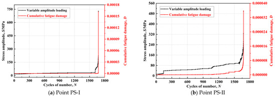
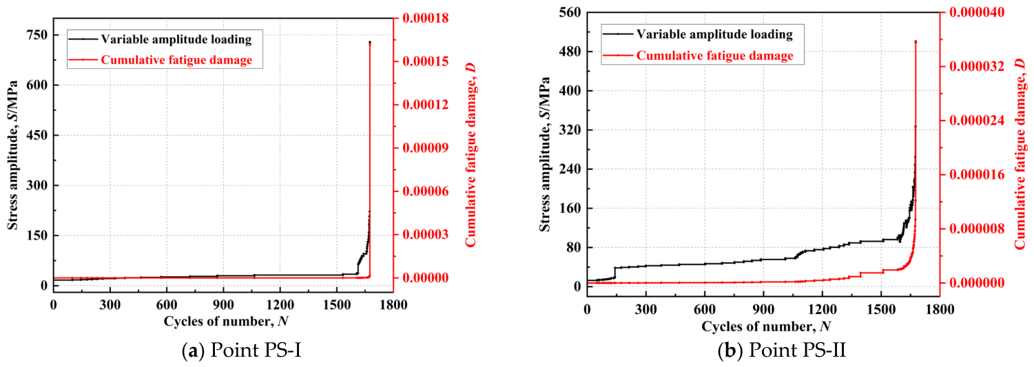
The rain–flow counted load levels are compiled into variable-amplitude load spectra. For each load level, the equivalent nominal stress is calculated using the modified Goodman equation. The corresponding allowable cycle count for each stress level is then determined from the material’s S-N curve. Fatigue damage per stress level is calculated, and the total cumulative damage over the statistical period is obtained by linear summation using the Palmgren–Miner rule, as detailed in Equations (17) and (18). The load spectra and accumulated fatigue damage for each critical point (uncracked condition) are presented in Figure 19. The results indicate that Critical Point I, located at the blade trailing edge-to-crown junction, sustains the highest fatigue damage. Consequently, this location is identified as the most probable site for the initiation of fatigue failure. The cumulative fatigue damage statistics for critical points without pre-existing cracks during the load rejection process are as follows: Critical Point PS-I exhibits a cumulative fatigue damage D of 1.62 × 10⁻⁴, while Critical Point PS-II shows a value of 3.57 × 10⁻⁵.

$$d_i={\displaystyle \frac{n_i}{N_i}}$$

(17)

$$D={\displaystyle \sum _{i=1}^n}{d}_i$$

(18)

where d_i represents the fatigue damage at different stress levels, n_i represents the number of cycles at the stress level, N_i represents the nominal number of cycles at the stress level, D represents the total fatigue damage.

Figure 19. Load spectrum and cumulative fatigue damage D during load rejection.

It should be noted that the Palmgren–Miner linear damage rule assumes linear accumulation, ignores load sequence and interaction effects, and neglects the fatigue limit. Nevertheless, it remains the most widely used method in engineering fatigue assessment and is considered appropriate for the comparative analysis between cracked and uncracked configurations under identical loading conditions in this study.

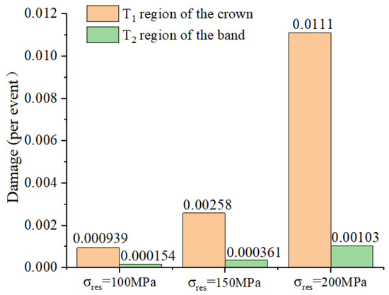
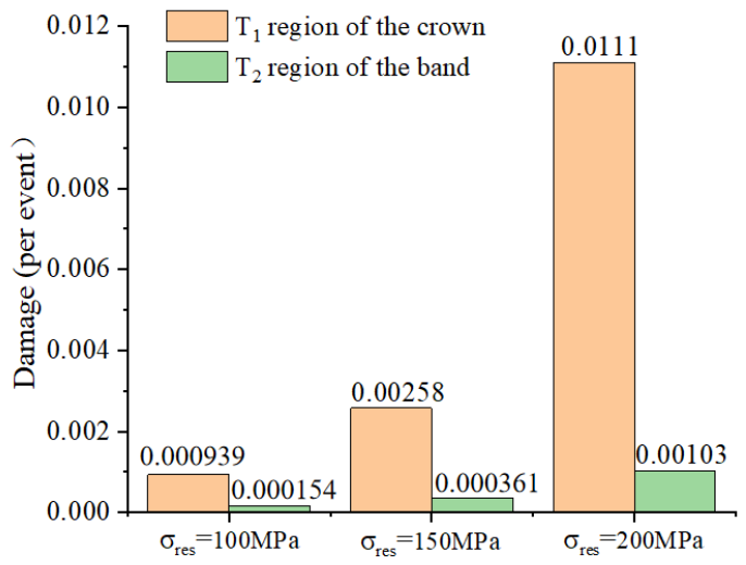
In the previous fatigue damage calculations, the residual tensile stress is approximately estimated to be 250 MPa. When pre-existing cracks are present at the T-joint, the original residual tensile stress may be further released. For the cracked runner, the residual stress is varied over a range of 100–250 MPa to account for different degrees of relaxation caused by the crack. The upper bound of 250 MPa corresponds to the limiting case of no relaxation, while the lower values (200, 150, and 100 MPa) represent progressively greater relaxation. This enables a systematic sensitivity analysis [36]. The fatigue damage calculation process for runners with pre-existing cracks is consistent with that for runners without cracks, so the load spectrum and cumulative damage process for runners with pre-existing cracks would not be detailed here. The cumulative fatigue damage statistics for runners with pre-existing cracks under different residual stresses during load rejection are shown in Figure 20. It could be seen that during the load rejection process, the critical points near the crown experience significantly higher fatigue damage than those near the band, indicating that runners with pre-existing cracks are more likely to experience fatigue failure at the connection between the blade trailing edge and the crown first. Additionally, under the same conditions, the fatigue damage of critical points decreases with the reduction of residual stress. Therefore, in practical engineering, it is possible to reduce the accumulation of fatigue damage by minimizing residual stress as much as possible.

Figure 20. Fatigue damage per load rejection in pre-cracked runners under varying residual stress.

According to the Palmgren–Miner linear cumulative damage hypothesis, fatigue failure occurs when the cumulative damage index D reaches the critical value of unity. Consequently, the fatigue life at each critical location can be predicted from the computed cumulative damage under the corresponding load spectrum. The relationship between these two quantities is given by Equation (19).

$$N={\displaystyle \frac{1}{D}}$$

(19)

where N denotes the fatigue life, expressed as the number of load rejection events, and D represents the cumulative fatigue damage accumulated during the statistical period.

The fatigue life of a Francis turbine runner is governed by the life at the critical point where the maximum fatigue damage occurs. Therefore, the fatigue life of the runner can be approximately estimated by calculating the fatigue life at the critical point that experiences the maximum cumulative fatigue damage, for both the uncracked and cracked configurations, as presented in the Table 3.

Table 3. Fatigue life estimation for uncracked and cracked runner configurations.

	Uncracked	With Pre-Existing Crack
Fatigue life, N	6173	100 MPa	150 MPa	200 MPa	Average fatigue life, NA
		1065	388	90	514

It can be observed that the presence of a pre-existing crack significantly reduces the fatigue life of the runner. The allowable number of load rejection events decreases from 6173 cycles for the uncracked runner to only 514 cycles for the cracked runner. This highlights the importance of regular inspection and maintenance of the runner during actual power plant operation. When cracks are detected, remedial measures such as weld repair can be adopted. However, the high residual stresses introduced in the repaired zone may substantially affect fatigue damage and should therefore be properly relieved.

4. Conclusions

(1) During load rejection, the rapid closure of guide vanes triggers a violent reorganization of the internal flow, characterized by the formation, evolution, and fragmentation of a dual-vortex structure into irregular vortex clusters. This process severely disturbs the pressure distribution on blade surfaces and directly generates strong unsteady hydraulic loads.

(2) The pressure pulsations induced by vortex evolution exhibit broadband spectral characteristics dominated by the rotational frequency and the blade-passing frequency (15f_n). The pulsation amplitude shows step-like intensification at the switching point of the guide vane closing law (t = 7.62 s), with a secondary peak occurring at the instant of maximum rotational speed (t = 15.5 s). This high-intensity excitation directly translates into cyclic alternating stresses on the runner blades.

(3) Under defect-free conditions, the maximum equivalent stress concentrates at the trailing-edge T-joints, shifting from the band side to the crown side as rotational speed increases. The crown-side T-joint exhibits approximately 4.5 times higher fatigue damage (D = 1.62 × 10⁻⁴) than the band-side joint (D = 3.57 × 10⁻⁵), identifying it as the most vulnerable region.

(4) The introduction of a pre-existing crack does not alter the location of the maximum stress, but it significantly intensifies stress concentration and increases the maximum equivalent stress by 61.1% (from 178.49 MPa to 287.55 MPa). This substantial stress elevation reduces the allowable number of load rejection events from 6173 to 514 cycles.

Several limitations of this study should be acknowledged. First, direct experimental validation of the computed stress results is lacking, as strain-gauge measurements on the runner blades were not feasible under the current on-site testing conditions. Second, the crack size is limited to a single value of 4 mm with a fixed through-crack geometry, and therefore the influence of crack length and shape on fatigue damage has not been systematically examined. Third, the residual stress levels adopted in the fatigue analysis are estimated based on literature data rather than in situ measurements on the prototype runner.

Future work will benefit from the installation of telemetric strain monitoring systems on the prototype runner to further substantiate the numerical predictions. In addition, a broader range of crack sizes and geometries should be considered to evaluate their effects on stress concentration and fatigue life. Fracture-mechanics-based indicators, such as the stress intensity factor, will be incorporated into the stress analysis to provide a more realistic evaluation of crack-tip behavior and to better assess the propensity for crack propagation. Furthermore, crack propagation modeling using the Paris law, combined with cumulative damage assessment under multiple operating conditions, will be pursued to establish a more comprehensive framework for the fatigue life prediction of Francis turbine runners.

References

- Kougias, I.; Aggidis, G.; Avellan, F.; Deniz, S.; Lundin, U.; Moro, A.; Muntean, S.; Novara, D.; Pérez-Díaz, J.I.; Quaranta, E.; et al. Analysis of emerging technologies in the hydropower sector. Renew. Sustain. Energy Rev. 2019, 113, 109257. [Google Scholar] [CrossRef] [Scilit]
- Bénard, L.C.; Afara, S.; Monette, C.; Nennemann, B. Dynamic Stress Prediction during Load Rejections in Hydraulic Turbines. IOP Conf. Ser. Earth Environ. Sci. 2025, 1483, 012017. [Google Scholar] [CrossRef] [Scilit]
- Trivedi, C.; Agnalt, E.; Dahlhaug, G.O. Experimental Investigation of a Francis Turbine during Exigent Ramping and Transition into Total Load Rejection. J. Hydraul. Eng. 2018, 144, 04018027. [Google Scholar] [CrossRef] [Scilit]
- Egusquiza, E.; Valero, C.; Huang, X.X.; Jou, E.; Guardo, A.; Rodriguez, C. Failure investigation of a large pump-turbine runner. Eng. Fail. Anal. 2012, 23, 27–34. [Google Scholar] [CrossRef] [Scilit]
- Côté, P.; Dumas, G.; Moisan, É.; Boutet-Blais, G. Numerical investigation of the flow behavior into a Francis runner during load rejection. IOP Conf. Ser. Earth Environ. Sci. 2014, 22, 032023. [Google Scholar] [CrossRef] [Scilit]
- Presas, A.; Valentin, D.; Zhao, W.Q.; Egusquiza, M.; Valero, C.; Egusquiza, E. On the use of neural networks for dynamic stress prediction in Francis turbines by means of stationary sensors. Renew. Energy 2021, 170, 652–660. [Google Scholar] [CrossRef] [Scilit]
- Zhang, X.X.; Chen, Q.H.; Liao, J. Dynamic evolutions between the draft tube pressure pulsations and vortex ropes of a Francis turbine during runaway. Int. J. Fluid Mach. Syst. 2017, 10, 404–411. [Google Scholar] [CrossRef] [Scilit]
- Fu, X.L.; Li, D.Y.; Wang, H.J.; Zhang, G.; Li, Z.; Wei, X. Dynamic instability of a pump-turbine in load rejection transient process. Sci. China Technol. Sci. 2018, 61, 1765–1775. [Google Scholar] [CrossRef] [Scilit]
- Trivedi, C.; Cervantes, M.J.; Gandhi, B.K.; Dahlhaug, O.G. Transient pressure measurements on a high head model Francis turbine during emergency shutdown, total load rejection, and runaway. J. Fluids Eng. 2014, 136, 121107. [Google Scholar] [CrossRef] [Scilit]
- Zeng, W.; Yang, J.D.; Hu, J.H.; Yang, J. Guide-vane closing schemes for pump turbines based on transient characteristics in S-shaped region. J. Fluids Eng. 2015, 138, 051302. [Google Scholar]
- Sun, L.G.; Guo, P.C.; Yan, J.G. Transient analysis of load rejection for a high-head Francis turbine based on structured overset mesh. Renew. Energy 2021, 171, 658–671. [Google Scholar] [CrossRef] [Scilit]
- Luna-Ramírez, A.; Campos-Amezcua, A.; Dorantes-Gómez, O.; Mazur-Czerwiec, Z.; Muñoz-Quezada, R. Failure analysis of runner blades in a Francis hydraulic turbine—Case study. Eng. Fail. Anal. 2016, 59, 314–325. [Google Scholar] [CrossRef] [Scilit]
- Saeed, R.A.; Galybin, A.N.; Popov, V. Modelling of flow-induced stresses in a Francis turbine runner. Adv. Eng. Softw. 2010, 41, 1245–1255. [Google Scholar] [CrossRef] [Scilit]
- Zhu, D.; Tao, R.; Xiao, R.F.; Pan, L. Solving the runner blade crack problem for a Francis hydro-turbine operating under condition-complexity. Renew. Energy 2020, 149, 298–320. [Google Scholar] [CrossRef] [Scilit]
- Xiao, R.F.; Wang, Z.W.; Luo, Y.Y. Dynamic stresses in a Francis turbine runner based on fluid-structure interaction analysis. Tsinghua Sci. Technol. 2008, 13, 587–592. [Google Scholar] [CrossRef] [Scilit]
- Liu, P.H.; Huang, X.X.; Yang, T.Y.; Wang, Z.W. Flow-induced fatigue damage of large Francis turbines under multiple operating loads. Appl. Sci. 2024, 14, 12003. [Google Scholar] [CrossRef] [Scilit]
- Magnoli, M.V. Numerical Simulation of Pressure Oscillations in Large Francis Turbines at Partial and Full Load Operating Conditions and Their Effects on the Runner Structural Behavior and Fatigue Life. Doctoral Dissertation, Technische Universitat Munchen, Munich, Germany, 2014. [Google Scholar]
- Li, Z.J.; Wang, Y.J.; Li, T.H.; Liu, F.; Ji, J. The dynamic characteristics of the ultimate strength of a turbine runner blade under hydraulic excitation. Energy Sources Part A Recovery Util. Environ. Eff. 2019, 41, 3127–3137. [Google Scholar] [CrossRef] [Scilit]
- Wang, X.F.; Li, H.L.; Zhu, F.W. The calculation of fluid-structure interaction and fatigue analysis for Francis turbine runner. IOP Conf. Ser. Earth Environ. Sci. 2012, 15, 052014. [Google Scholar] [CrossRef] [Scilit]
- Zhang, M.; Valentin, D.; Valero, C.; Egusquiza, M.; Zhao, W. Numerical study on the dynamic behavior of a Francis turbine runner model with a crack. Energies 2018, 11, 1630. [Google Scholar] [CrossRef] [Scilit]
- Gagnon, M.; Tahan, A.; Bocher, P.; Thibault, D. On the Fatigue Reliability of Hydroelectric Francis Runners. Procedia Eng. 2013, 66, 565–574. [Google Scholar] [CrossRef] [Scilit]
- Yang, J.; Pavesi, G.; Liu, X.H.; Xie, T.; Liu, J. Unsteady flow characteristics regarding hump instability in the first stage of a multistage pump-turbine in pump mode. Renew. Energy 2018, 127, 377–385. [Google Scholar] [CrossRef] [Scilit]
- Lu, Y.G.; Xin, L.C.; Hu, N.M.; Zhu, Z.; Xia, W. Influences of floating ice on the water entry process of slender body on the cavity evolution and hydrodynamic characteristic. Phys. Fluids 2025, 37, 042103. [Google Scholar] [CrossRef] [Scilit]
- Yang, J.; Zheng, Y.Y.; Wang, J.Z.; Feng, X.; Zhang, J.; Liu, X. Compressibility effects and rotational dynamics of stall cells in a pump turbine diffuser during hump instability. Phys. Fluids 2025, 37, 056102. [Google Scholar] [CrossRef] [Scilit]
- Yan, J.P.; Koutnik, J.; Seidel, U.; Hubner, B. Compressible Simulation of Rotor-Stator Interaction in Pump-Turbines. Int. J. Fluid Mach. Syst. 2010, 3, 315–323. [Google Scholar] [CrossRef] [Scilit]
- Kan, K.; Yu, Y.K.; Zhou, Y.G.; Chen, Y.; Ye, C. Numerical investigation of multiscale flow-induced vibration and fatigue life prediction of a large Francis turbine. Energy 2025, 335, 138334. [Google Scholar] [CrossRef] [Scilit]
- Bathias, C.; Pineau, A. (Eds.) Fatigue of Materials and Structures: Application to Design and Damage; John Wiley & Sons, Inc.: Hoboken, NJ, USA, 2013. [Google Scholar]
- Lyutov, A.; Kryukov, A.; Cherny, S.; Chirkov, D.; Salienko, A.; Skorospelov, V.; Turuk, P. Modelling of a Francis Turbine Runner Fatigue Failure Process Caused by Fluid-Structure Interaction. IOP Conf. Ser. Earth Environ. Sci. 2016, 49, 072012. [Google Scholar] [CrossRef] [Scilit]
- Huang, Y.H.; Mi, Y.D. Research on Fatigue Performance of Steel for Turbine Runners. Large Electr. Mach. Hydraul. Turbine 1985, 6, 50–55+2. (In Chinese) [Google Scholar]
- Yang, X. Sanxia Runner Fatigue Analysis. Master’s Thesis, Southwest Jiaotong University, Chengdu, China, 2006. [Google Scholar]
- Li, W.; Zhang, L.D. Methods of Estimating the fatigue life of a Francis turbine runner. Friend Sci. Amat. 2010, 4, 3–5. [Google Scholar]
- Chang, H.; Wang, Z.Q.; Peng, G.J.; Shi, W.; Lin, R.; Zhou, L. Role of wall roughness on energy dissipation and vortex dynamics in self-priming centrifugal pump: A study via entropy generation and Liutex vortex identification. Energy 2025, 337, 138733. [Google Scholar] [CrossRef] [Scilit]
- Lu, Y.G.; Liu, Z.W.; Zhao, Y.; Wang, Z.; Presas, A. Study on evolution characteristics of energy dissipation and vortex in pump-turbine during load rejection transition process. Phys. Fluids 2025, 37, 025104. [Google Scholar] [CrossRef] [Scilit]
- Lu, Y.G.; Li, X.L.; Yi, C.; Meng, Q.; Presas, A. Study of energy dissipation dynamics and pressure fluctuation response during pump-turbine startup in pump mode. Phys. Fluids 2025, 37, 115121. [Google Scholar] [CrossRef] [Scilit]
- Wang, J.Q.; Wang, R.Z.; Zhang, R.Y.; Lu, Y.; Wang, D.; Fu, Q. Prediction of stress-fatigue life on the impeller of the reactor coolant pump based on fluid-thermal-structure interaction method. Ann. Nucl. Energy 2023, 193, 110029. [Google Scholar] [CrossRef] [Scilit]
- Cheng, G.F.; Wei, S.; Wen, D.W.; Li, Z. New equipment and method for measuring welding residual stress in Francis runner. Trans. China Weld. Inst. 2013, 34, 67–70. [Google Scholar]
Disclaimer/Publisher’s Note: The statements, opinions and data contained in all publications are solely those of the individual author(s) and contributor(s) and not of MDPI and/or the editor(s). MDPI and/or the editor(s) disclaim responsibility for any injury to people or property resulting from any ideas, methods, instructions or products referred to in the content. |
© 2026 by the authors. Licensee MDPI, Basel, Switzerland. This article is an open access article distributed under the terms and conditions of the Creative Commons Attribution (CC BY) license.