


Abstract
To address the limitations of single-modality feature characterization in tool wear monitoring, as well as the susceptibility of deep regression models to local optima and their poor robustness under complex working conditions, this paper proposes a tool wear prediction method based on a multimodal attention mechanism and interval guidance. First, a Region of Interest (ROI) algorithm removes visual background redundancy, constructing an adaptive ROI-based visual stream feature model to achieve spatial alignment across image dimensions. Concurrently, the Gramian Angular Field (GAF) is introduced to encode one-dimensional acoustic emission signals into two-dimensional time-frequency feature maps. Subsequently, utilizing the EfficientNetV2 backbone network, Bi-Directional Cross-Attention (BCA) is employed to facilitate deep interaction between visual and acoustic features, ensuring cross-modal semantic alignment. Second, interval classification is introduced as an auxiliary constraint to guide the model toward precise localization within the fine-grained regression space, while a priori constraints are applied to this feature space. To mitigate task weight uncertainty, a Stable Kendall Loss is utilized to adaptively balance the weights among the global regression, interval classification, and structured regression tasks. Finally, the proposed model is experimentally validated using the MATWI dataset. Experimental results demonstrate a classification accuracy of 94.58% and a minimum mean absolute error (MAE) of 6.6183 μm. Compared to state-of-the-art prediction methods and official benchmarks, the proposed model achieves superior performance across all evaluation metrics. Notably, it reduces prediction errors by approximately 65% relative to the benchmark model, fully validating its high accuracy and robust performance under complex working conditions.
1. Introduction
As we move toward Industry 4.0, precision manufacturing demands increasingly stringent machining quality and high production efficiency. Because tools are the core executing components of a cutting system, their health directly determines the dimensional accuracy and surface integrity of the workpiece. Statistics indicate that unplanned downtime caused by tool wear and failure accounts for approximately 20% of total CNC machine tool downtime. The resulting increase in production costs and resource waste has become a bottleneck restricting the high-quality development of manufacturing. Therefore, constructing high-precision, robust tool condition monitoring systems has become a critical component of intelligent production. With the rapid advancement of deep learning technologies, data-driven monitoring methods have gradually superseded traditional physics-based approaches. As highlighted by several recent comprehensive reviews on Tool Condition Monitoring (TCM) [1,2], the research frontier has definitively shifted from single-sensor feature engineering to deep multimodal fusion. However, in complex industrial environments, existing single-modality monitoring methods often struggle to balance comprehensiveness and reliability, further confirming the necessity of integrating visual images with dynamic sensor signals as pointed out in recent literature. Although multimodal fusion offers the advantage of information complementarity, practical applications present new challenges in tool wear prediction: achieving semantic alignment of heterogeneous data, managing the nonlinear dynamic characteristics of wear evolution, and balancing conflicts during multitask optimization.
In the feature extraction of multimodal signals, heterogeneous feature encoding and spatial alignment techniques form the foundation for constructing robust feature spaces. In early research, Wang et al. [3] utilized convolutional neural networks (CNNs) to directly extract features from one-dimensional cutting force signals. While this demonstrated the potential of deep models in handling complex non-stationary signals, it often overlooked the internal temporal dependencies and topologies of the signals. Subsequently, Zhou, Y and Xue, W. [4] introduced the Gramian Angular Field (GAF) transformation, mapping one-dimensional time series to polar coordinates to generate two-dimensional images. This effectively preserved the temporal correlations of the signals and improved the model’s accuracy in recognizing early wear patterns. However, GAF encoding often suffers from phase asymmetry issues caused by variations in physical installation positions when processing data from multi-channel sensors. To address this limitation, Guo et al. [5] proposed a multi-channel wide-kernel wavelet convolution architecture, utilizing continuous wavelet basis functions to initialize the convolution kernels and achieve preliminary alignment of heterogeneous signals within specific frequency bands. Building upon this, Pan et al. [6] explored feature distortion caused by differences in sensor layouts. They employed Bayesian estimation to apply uncertainty quantification across multiple physical channels, achieving probabilistic spatial alignment of cross-modal features. Despite these advancements in dimensional unification, existing feature encoding methods remain highly susceptible to environmental noise in highly dynamic machining scenarios. Furthermore, establishing strict physical spatial consistency across multimodal data remains difficult, thereby limiting the construction of effective feature spaces.
Once multimodal features are initially aligned, the primary challenge becomes bridging the semantic gap between visual and acoustic modalities to achieve deep cross-modal information interaction. Traditional fusion strategies primarily rely on simple feature-level concatenation. Yang et al. [7] demonstrated that while this static fusion method is straightforward, it is easily misled by a single noisy modality during abrupt changes in cutting conditions, as it lacks a dynamic weighting mechanism between modalities. To enhance interaction depth, Cheng et al. [8] proposed Swin-Fusion, a Transformer-based fusion network that utilizes local and global feature exchange mechanisms to improve the capture of dynamic wear processes. However, the standard Transformer self-attention mechanism primarily focuses on intra-modality dependencies and struggles to explicitly address the phenomenon of “physical dislocation” between modalities. To overcome this, Chai et al. [9] introduced CABLSTM, a combination of bidirectional long short-term memory (Bi-LSTM) networks and attention mechanisms. This model identifies the critical transition point from steady-state to severe tool wear through bidirectional modeling; however, gaps remain in the cross-validation of different physical sensor attributes. Subsequently, Zhang et al. [10] proposed a cross-attention-based decoupling method, which preliminarily resolved the ambiguity of composite fault features by establishing bidirectional semantic mapping between signals and images.
At the prediction layer, modeling the phased nonlinear characteristics of wear evolution is crucial for improving tool wear prediction accuracy. Tool degradation generally follows a standard bathtub curve, whereas traditional end-to-end regression models often mistakenly treat wear as a single linear cumulative process. Sun et al. [11] pointed out that without integrating physical degradation mechanisms, this linear mapping tends to cause significant overshoot errors during the acute failure stage. To address this, they proposed Physics-Informed Gaussian Process Regression (PIGPR) to narrow the prediction’s confidence intervals. Wu et al. [12] introduced manifold regularization to unlabeled samples to generate pseudo-labels. By employing a Long Short-Term Memory (LSTM) network, the model learns correlations across different evolutionary intervals, thereby more precisely fitting the nonlinear dynamic features of the tool from stable wear to rapid degradation. However, enabling the model to autonomously adjust the slope of the prediction interval under variable machining parameters remains a challenge. Addressing this, Li et al. [13] achieved zero-shot transfer of the monitoring model across multiple working conditions by inputting cutting parameters as external conditions, thereby enhancing the model’s adaptive perception of nonlinear degradation rates. He et al. [14] established a 0.10 mm failure threshold and utilized the multilayer features of a Symmetrized Dot Pattern (SDP) to clearly define wear states, providing a reliable decision-making basis for preventive tool replacement.
Balancing the convergence speeds of numerical regression and interval classification across different dimensions is crucial. Traditional fixed-weight loss function stacking frequently leads to gradient dominance, where gradients from simple tasks overwhelm those from complex tasks. Kendall et al. [15] proposed a multi-task learning principle based on homoscedastic uncertainty, arguing that task weights should be dynamically determined by their inherent noise levels. Subsequently, Li et al. [16] applied this theory in WaveletKernelNet to achieve dynamic adaptive allocation of multi-task losses. By evaluating the inherent noise differences among multidimensional tasks, this approach effectively prevented single-task dominance in network gradient updates. Sun et al. [17] proposed a dynamic constrained uncertainty weighting (DRUW) strategy that attenuates the loss contributions of abnormal task branches by monitoring input quality in real time. This ensures gradient collaboration and stable convergence during the joint optimization of complex multi-task architectures.
In summary, while existing research has made significant progress in dimensional unification and preliminary multimodal fusion, a critical gap remains in the literature: existing studies largely isolate the structural design of multimodal fusion from the dynamic physical stages of tool degradation. Although individual techniques—such as GAF, cross-attention, and multi-task learning—have been explored independently, there is a lack of a unified framework that mathematically couples the causal verification of heterogeneous sensor data with the highly nonlinear trajectory of physical wear.
To bridge this gap, this paper proposes a novel tool wear prediction network that synergistically integrates visual-acoustic cross-attention with interval guidance. Rather than merely stacking known modules, this study couples visual geometry and acoustic dynamics into a closed-loop causal verification system. Furthermore, to ensure the proposed architecture is evaluated under authentic industrial conditions, this study leverages the Multimodal Automatic Tool Wear Inspection (MATWI) benchmark dataset [18]. This dataset was specifically selected because it uniquely provides synchronously aligned, high-resolution optical images of tool inserts and continuous high-frequency acoustic emission sequences collected during actual CNC milling operations. Unlike conventional datasets that provide only isolated 1D signals or standalone static images, the synchronous multimodal nature of MATWI perfectly matches the input requirements of our visual-acoustic cross-verification mechanism, providing a rigorous physical foundation for validating the proposed framework. The original contributions of this study are explicitly summarized as follows:
- A Novel Bidirectional Causal Fusion Framework: Unlike traditional static concatenation or standard self-attention, we propose a Bidirectional Cross-Attention (BCA) mechanism to explicitly address the semantic misalignment between heterogeneous sensors. By utilizing acoustic dynamics to reverse-verify visual features (and vice versa), this mechanism establishes a physical causality loop. It effectively filters out unilateral environmental noise and transient vibration artifacts, ensuring deep semantic alignment across modalities without relying on simple feature stacking.
- Physics-Informed Interval-Guided Learning (IGL): To address the predictive lag of traditional end-to-end regression models during severe wear stages, we introduce a dual-layer cognitive framework. By converting known physical wear intervals into a Gaussian soft-labeling space, coarse-grained physical state classifications are dynamically used to gate fine-grained expert regression heads, ensuring continuous smoothness across the tool’s lifecycle.
- Uncertainty-Adaptive Multi-Task Optimization for Tool Wear: While traditional multi-task networks frequently suffer from gradient dominance, we uniquely tailored a homoscedastic uncertainty-based loss strategy to orchestrate our specific tri-branch architecture (global regression, interval gating, and local expert regression). Instead of relying on blind manual hyperparameter tuning, this mechanism mathematically quantifies the intrinsic noise of each physical task to dynamically resolve dimensional discrepancies. By continuously modulating task weights, it prevents simple tasks from overwhelming complex ones during abrupt wear transitions, thereby mathematically guaranteeing the highly synergistic convergence of qualitative wear state identification and quantitative wear depth prediction.
2. Methods
In CNC milling, tool wear is a complex, nonlinear physical degradation process typically characterized by an “inverse S-curve” comprising three stages: initial break-in, stable wear, and severe wear [19]. During the cutting process, physical phenomena such as abrasive friction, adhesive peeling, and localized micro-chipping continuously alter the tool’s geometric morphology and contact stiffness [20].
Effective condition monitoring relies on capturing these physical changes through appropriate sensor signals. However, under highly complex cutting conditions, single-modality perception often struggles to balance early detection with precise quantification. Different monitoring modalities capture distinct physical attributes of the wear process, presenting an inherent physical complementarity:
Visual Signals: Optical images directly record the macroscopic geometric defects of the tool, such as the flank wear width (VB) and chipping area. This provides highly intuitive, robust spatial localization and state quantification capabilities [21]. However, visual inspection is often intermittent, susceptible to occlusion by cutting fluids or industrial lighting, and suffers from significant latency in early detection, making it difficult to identify incipient hidden wear.
Acoustic Emission (AE) Signals: In contrast to static geometry, AE signals capture the high-frequency dynamic responses of the cutting process. Extremely sensitive to microscopic material fracture, plastic deformation, and crack propagation [22], AE enables the continuous, real-time capture of subtle incipient deterioration and transient shocks that vision might miss. While demonstrating strong resistance to physical occlusion, these signals are highly vulnerable to background noise in the workshop environment, making it challenging to precisely quantify wear conditions relying on acoustics alone.
Therefore, robust tool condition monitoring fundamentally requires solving a dual-challenge engineering problem: how to simultaneously capture macroscopic geometric deformation and microscopic dynamic shocks while effectively resisting industrial environmental noise. By leveraging the physical complementarity between macroscopic geometry and microdynamics, the subsequent sections propose a tool wear monitoring method based on visual-acoustic dual-modality fusion. Utilizing cross-attention and interval guidance, this comprehensive engineering solution aims to balance the early detection of tool deterioration with the precise quantification of subsequent wear, thereby enhancing the extraction and prediction of multi-scale wear features under complex working conditions.
2.1. Heterogeneous Feature Coding and Spatial Alignment
When constructing multimodal tool wear monitoring models, directly performing deep feature fusion on raw heterogeneous data often leads to severe dimensional mismatches and semantic misalignment. Visual and acoustic modalities differ not only in their physical dimensions and sampling structures but also in their sensitivity to specific degradation features, which are easily obscured by complex and variable machining noise. To fundamentally address this critical challenge in multimodal representation, a systematic architecture for heterogeneous feature encoding and spatial alignment is constructed. The core objective of this architecture extends beyond simple noise reduction. Instead, it rigorously establishes spatial geometric anchors for the target at the physical representation level, while achieving cross-dimensional mapping from one-dimensional temporal dynamics to two-dimensional spatiotemporal textures at the data structure level. Through such regularization and reconstruction at the shallow input layer, the visual and acoustic modalities are mapped into a homogeneous perceptual dimension. This provides a reliable data foundation for subsequent deep cross-modal feature fusion.
EfficientNetV2 was specifically selected as the visual backbone over ResNet or Vision Transformers (ViT) due to its optimal balance between parameter efficiency and spatial extraction capability. Unlike ViTs, which lack inductive biases and require massive datasets to converge—making them prone to overfitting on limited industrial datasets (e.g., ~1600 samples in MATWI)—EfficientNetV2 utilizes Fused-MBConv convolutions to robustly extract localized geometric defects (e.g., micro-chipping) with a highly lightweight architecture, which is crucial for real-time deployment.
2.1.1. Visual Stream Image Data Processing
In the multimodal condition monitoring system, the visual stream is responsible for capturing micro-texture changes and macroscopic geometric defects of the tool edge. However, as represented by the “Raw Image” block in the pipeline (Figure 1), the original images captured directly from the CNC machine (e.g., from the MATWI dataset) are not clean isolated tools; they contain massive amounts of industrial background interference, such as complex spindle structures, cutting fluid splatter, and uneven light reflections on metal surfaces. If these raw images are directly fed into deep neural networks, the high-frequency background noise will severely dilute the feature weights of the target tool wear area [23].
Figure 1.
The raw images in the MATWI dataset.
Therefore, strict spatial preprocessing is mandatory. To address this, we construct an adaptive Region of Interest (ROI) extraction pipeline. It should be noted that while the fundamental image processing operators used in this pipeline—such as Gaussian smoothing and Canny edge detection—are standard methods adopted from classical computer vision literature [24], our original contribution lies in the design of the adaptive dual-threshold mechanism (Equation (2)) and the dynamic convex-hull elastic bounding logic (Equation (3)), which are specifically tailored to reliably isolate tool bodies under variable industrial illumination. The raw image data of the MATWI dataset are presented in Figure 1.
First, to overcome challenges such as the anisotropy of metal surface textures, significant light intensity variations across processing batches, and the limitations of fixed-threshold segmentation, the input RGB images are converted into grayscale images and smoothed using a Gaussian filter. This preprocessing step suppresses speckle noise caused by metal grains. The definition of the Gaussian kernel function is as follows:
After this smoothing preprocessing, the resulting image is fed into an improved Canny edge detection operator. To ensure the algorithm accurately captures abrupt gradient boundaries between the tool contour and the background under both overexposed and underexposed conditions, an adaptive edge gradient dual-threshold strategy is introduced. Based on global pixel brightness, this strategy dynamically calculates the low threshold and high threshold for the Canny operator to generate a robust binary edge map strategy based on global pixel brightness to dynamically construct the Canny operator:
where is a floating-point coefficient and represents the median pixel intensity of the image.
Tool contours extracted via edge detection are often discontinuous; this is especially true in severely worn areas where chipping causes edge fragmentation. To construct a complete tool mask, morphological closing—an operation consisting of dilation followed by erosion—is employed to connect fractured edges and fill small holes.
Subsequently, the contour and ROI extraction module determines the main position of the tool by identifying the maximum connected domain and computing its convex hull. The convex hull set is defined as the smallest convex polygon containing the tool contour point set denoted as . The physical significance of using the convex hull lies in its ability to accommodate irregular geometric deformations caused by severe tool wear or chipping. This ensures that the extracted area consistently and completely covers the tool tip, the flank face, and part of the rake face, thereby avoiding missed detections.
After obtaining the geometric convex hull of the tool, the algorithm calculates its bounding rectangle to serve as the initial ROI. To prevent the loss of tool tip edge information during subsequent convolution operations, a padding ratio is introduced around the bounding box to generate an elastic boundary prior to cropping. The corrected cropping coordinates are calculated as follows:
where is the padding ratio (set to 5%), are the coordinates of the initial bounding rectangle, and (x’, y’, w’, h’) are the corrected cropping coordinates. The selection of was determined based on empirical testing during the image preprocessing phase. Sensitivity observations indicated that a smaller padding ratio (e.g., <3%) risks truncating irregular and severe wear features—such as micro-chipping at the tool tip—due to the bounding box fitting too tightly. Conversely, a larger ratio (e.g., >10%) introduces excessive background interference, which dilutes the spatial focus of the visual backbone network. Therefore, 5% was established as an optimal threshold to preserve a safe elastic boundary for morphological complete wear states while strictly controlling background redundancy.
The cropped tool image is uniformly resized to 384 × 384 dimensions using bilinear interpolation. This process achieves spatial alignment; regardless of slight variations in focal length or tool position during the original image capture, the network input is consistently a centrally positioned and uniformly sized tool body. Subsequently, this standardized visual tensor is fed into the visual backbone network for deep spatial feature extraction. To extract global semantic information and compress the spatial dimensions, the terminal layers of the network sequentially perform adaptive global pooling and feature flattening. This ultimately generates a global visual feature vector which encapsulates the macroscopic geometry and microscopic texture states of the tool. This vector serves as the core semantic anchor for the subsequent multimodal cross-attention mechanism. The specific visual processing workflow for the adaptive ROI is illustrated in Figure 2.
Figure 2.
Visual Flow Processing Workflow for Adaptive ROI.
2.1.2. Acoustic Flow Sensor Data Processing
The raw sensor signal acquired during milling is a one-dimensional, highly non-stationary high-frequency time series (as visualized later in Section 3). It contains rich information regarding microscopic friction and stress wave propagation [25]. However, directly merging this 1D temporal sequence with 2D visual features leads to severe dimensional mismatches.
To resolve this, we map the acoustic signals into 2D spatiotemporal textures. In this module, the Gramian Angular Field (GAF) transformation (Equations (5)–(7)) is a standard time-frequency encoding method adopted from existing literature, widely recognized for losslessly preserving temporal dependencies [26]. However, our original contribution in this stream is the preceding Adaptive Channel Selection and Fourier-based Global Resampling mechanism (Equation (4)). This original mechanism ensures that the GAF transformation is fed with the most dynamically rich cutting sequences rather than fixed channels that may suffer from sensor failure or transient noise. Furthermore, the Fourier-based global resampling losslessly standardizes the input sequence length, which effectively prevents high-frequency aliasing and preserves the complete global cutting dynamics that are frequently discarded by traditional fixed-window segmentation.
Adaptive Channel Selection Mechanism
Sensor data collected from industrial environments typically comprises multiple channels, with signal-to-noise ratios varying significantly under different operating conditions. Because previous studies have demonstrated that acoustic emission signals are highly sensitive to the initiation of early microscopic cracks and high-frequency microscopic shocks [27,28,29], the proposed algorithm prioritizes the selection of acoustic emission channels. If a designated channel is missing or data anomalies are detected, an adaptive selection mechanism is triggered. This mechanism is based on the information-theoretic principle that a larger variance indicates a signal channel containing richer cutting dynamics—such as transient shocks caused by severe vibrations or tool chipping [30]—rather than smooth background noise. Therefore, the algorithm calculates the variance of all valid data channels and dynamically selects the one with the maximum variance as the input:
where is the target channel, is the variance of channel , and represents the set of all active sensor channels.
To avoid aliasing caused by time-domain downsampling and to prevent the loss of transient high-frequency components associated with tool wear, a Fourier transform-based resampling technique is applied to the selected signal sequence . This technique adjusts the signal length in the frequency domain to a target size of N = 128, yielding the reconstructed one-dimensional signal , which preserves high-frequency features and unifies the input scale.
To map the reconstructed one-dimensional signal into a two-dimensional space, the values are first normalized and strictly constrained to the range [−1, 1]. The transformation formula for the normalized sequence is:
Subsequently, a polar coordinate encoding system is introduced to map the normalized values to angular representations , while timestamps are mapped to the radius .
Based on this representation, the Gramian Angular Field (GAF) matrix is computed using the trigonometric sum of angles for any two time points and :
The main diagonal elements correspond to , preserving the amplitude information of the original signal at a given moment ; The off-diagonal elements encode the temporal correlations between different time steps.
The generated GAF images are fed into a specially designed lightweight convolutional neural network (SensorCNN). This network comprises three convolutional blocks, each containing 3 × 3 convolution kernels, a GELU activation function, and a 2 × 2. max pooling layer. The number of channels in the feature maps increases progressively layer by layer. Ultimately, the features are mapped to a 256-dimensional vector through an adaptive average pooling layer and a fully connected layer .
This network architecture not only effectively extracts multi-scale texture features from the GAF images but also projects the sensor data directly into a 256-dimensional latent semantic space that is consistent with the visual stream dimensions. This deep semantic alignment lays the mathematical foundation for the subsequent cross-attention-based multimodal feature fusion. As illustrated in Figure 3, the acoustic stream processing module takes the raw 1D sensor data as input. Through adaptive channel selection, FFT resampling, and GAF mapping (Equations (5)–(7)), it converts the signal into a 2D spatiotemporal texture. The SensorCNN then projects this texture into a 256-dimensional latent space, yielding the aligned Acoustic Feature Vector (). This output vector subsequently acts as the Key/Value input for the cross-attention mechanism detailed in the next stage.
Figure 3.
Acoustic flow processing flow based on GAF.
2.2. Bidirectional Cross-Attention Mechanism
In multimodal tool wear monitoring, although visual and acoustic modalities are highly complementary, an essential semantic gap exists between them. Visual data captures the flank wear width (VB) and chipped edge geometry through high-resolution spatial pixel matrices, providing strong spatial localization. Conversely, acoustic data, despite being mapped to two dimensions by the GAF in shallow layers, inherently records frictional vibration and stress wave energy as a time series, exhibiting exceptionally high temporal sensitivity. To address semantic misalignment during the fusion of heterogeneous features, this paper constructs a BCA mechanism at the feature fusion layer, inspired by recent advancements in cross-modal collaborative alignment [31,32,33].
To explicitly distinguish the proposed BCA from standard attention mechanisms, we articulate its mathematical and structural differences. Standard self-attention derives its Query (), Key (), and Value () matrices from a single modality (e.g., ), strictly capturing intra-modal dependencies without addressing cross-modal interactions. Furthermore, typical cross-attention employed in conventional fusion frameworks is predominantly unidirectional—mapping modality to query modality (). Mathematically, this calculates a singular attention map , which merely injects ’s features into ’s semantic space while ignoring the reciprocal causal verification of based on .
In contrast, the proposed BCA employs a symmetric dual-query architecture to strictly enforce bidirectional physical causality. Mathematically, it concurrently computes dual attention maps and . By integrating independent residual connections in both pathways, the output mathematically preserves both original modal identities enriched by reciprocal verification: . This dual-residual mathematical structure forces the network to learn bidirectional physical causalities—using visual geometry to retrieve acoustic dynamics and acoustic energy to eliminate visual illusions—rather than simply substituting or overwriting one modality with another.
Furthermore, we clarify how the model strictly preserves and utilizes temporal dependencies without relying on the network layers to explicitly learn chronological order. In our framework, the one-dimensional acoustic emission sequence is first transformed via the polar coordinate system of the Gramian Angular Field (GAF) prior to feature fusion. In the GAF matrix , the row index and column index strictly map to the absolute timestamps of the raw signal, where the main diagonal retains the chronological sequence of amplitudes and the off-diagonal elements explicitly encode the inner-product temporal correlations between different time steps. Consequently, temporal dependencies are losslessly mapped into localized two-dimensional spatial-temporal textures, which are subsequently captured by the downstream SensorCNN utilizing its localized receptive fields. Therefore, the latent semantic vectors input into the BCA mechanism are already thoroughly contextualized with rich temporal characteristics. The role of the BCA mechanism is not to explicitly extract sequence order, but to perform higher-level causal cross-verification on these feature vectors that have already successfully encapsulated temporal attributes.
2.2.1. Visually Guided Acoustic Pathways
Image-to-sensor attention plays a crucial role in semantic anchoring. The core logic of this pathway utilizes visual geometric features as active query vectors. These vectors retrieve and enhance spectral components strongly correlated with the current wear state from an acoustic feature space laden with environmental noise and redundant information, thereby achieving precise cross-modal alignment.
Because macroscopic physical damage on the tool surface generates specific acoustic emission signals [34,35,36], visual features are employed as indices for the cross-retrieval of acoustic features. This approach fundamentally explores nonlinear acoustic characteristics that correspond to the visual damage. Specifically, the global visual feature vector , extracted and projected by the EfficientNet backbone network, serves as active guidance. Here, represents the batch size and denotes the latent semantic dimension. The visual feature matrix is mapped to the query matrix , while the acoustic feature vector , encoded by SensorCNN, is mapped to the key and value matrices. During computation, the original features are first projected onto a common semantic subspace using linear transformation matrices:
Here, represent the independent learnable parameter matrices for the visually guided acoustic pathway.
Because the input features are globally pooled single vectors, their dimensions are reshaped into a pseudo-sequence format via dimensionality expansion to satisfy the sequence input requirements of multi-head attention. This treats the entire tool sample as an inseparable time step, allowing the attention mechanism to focus on sample-level global feature associations.
The core of this pathway involves calculating the dot-product similarity between the visual queries and acoustic keys , to construct a cross-modal attention map. This process quantifies the physical compatibility between the observed wear patterns and the collected acoustic features. The standardized attention weight is calculated as follows:
Here, is the scaling factor of the feature dimension, and is the transposed key matrix. Transposing the key matrix enables the visual stream to traverse and retrieve various dynamic components within the acoustic stream. This calculates their physical correlations, thereby determining which relevant physical features to retain and which conflicting noise features to discard. Notably, because the sequence length is 1, the Softmax activation function operates along the feature channel dimension. This achieves fine-grained, adaptive weighting of the -dimensional dynamic spectral components, rather than performing traditional sequence time-step weighting.
In tool wear monitoring scenarios, this weight matrix exhibits clear physical directionality. For instance, if a severe triangular chip at the tool tip is detected visually , the resulting query vector interacts with the high-dimensional acoustic space via dot-product operations. Consequently, characteristic components representing high-frequency transient shocks receive significantly higher attention weights. Conversely, if visual data indicate uniform flank wear, the attention mechanism focuses on retrieving low-frequency energy features from the acoustic signal that represent steady-state friction. This mechanism automatically assigns greater weight to features with high physical consistency, effectively suppressing industrial background noise and physical artifacts. Because these noise signals lack a corresponding visual geometric source, their dot-product activation values remain extremely low.
After obtaining the attention weights, the algorithm performs a weighted aggregation of the acoustic value matrix Furthermore, this study employs a multi-head attention mechanism with 4 heads to execute parallel computation and aggregation across four independent subspaces. The outputs of each head are concatenated to produce the final visually calibrated acoustic features :
The specific workflow of this visually guided acoustic pathway is illustrated in Figure 4. The primary purpose of this module is to utilize the robust spatial geometry of the tool (Visual Feature Vector ) as a Query to cross-reference the acoustic stream. Through linear projections (Equation (8)) and attention weight calculations (Equation (9)), the module explicitly filters out unverified environmental noise. The final output is the Enhanced Acoustic Features (Equation (10)). Physically, the term “Enhanced Acoustic Features” represents a purified set of dynamic acoustic signals that are strictly corroborated by actual visual wear defects (e.g., high-frequency chipping sounds perfectly aligned with a missing tool tip), thereby eliminating random machine vibrations from the semantic space.
Figure 4.
Visual-guided acoustic flowchart.
2.2.2. Acoustic Guidance of Visual Pathways
This pathway is structurally symmetrical to the visually guided pathway. It aims to perform reverse causal verification of geometric artifacts within visual features by utilizing physical quantities, such as contact stiffness and cutting energy, embedded in the acoustic features.
In this pathway, the acoustic feature vectors , encoded deeply via the GAF transformation and SensorCNN, no longer serve as passive auxiliary variables. Instead, they are linearly mapped into query matrices that control the global attention distribution. Correspondingly, the visual feature vectors , which are rich in texture details, are mapped into key and value matrices. Every acoustic event generated during the cutting process should theoretically have a corresponding geometric representation in the visual image. If the acoustic signal is smooth, any visual anomaly is likely attributable to illumination noise. Conversely, if the acoustic signal exhibits a strong impact transient, the visual features must focus on potential chipping areas. This design enables the query matrix to represent the current cutting force within a high-dimensional semantic space, facilitating the retrieval of matching geometric damage from the image features. The projection transformation is formulated as follows:
Here, , represent the independent learnable parameter matrices for the acoustically guided visual pathway.
The core of this attention mechanism involves calculating the alignment between the acoustic queries and visual keys to generate cross-modal attention weights. The standardized attention weight is calculated as follows:
Essentially, this process conducts cross-modal causality verification. Under actual tool wear monitoring conditions, Equation (12) correlates with specific physical scenario identifications. For example, if the sensor captures typical high-frequency, transient acoustic emission signals, it usually indicates the occurrence of a brittle fracture. In this case, carries the semantic vector corresponding to the brittle fracture. If the visual keys () represent an intact tool tip or cutting edge, a semantic mismatch occurs, resulting in low dot-product activation values for . However, if , if the corresponding texture is shell-like peeling on the post-tool surface, the two are highly collinear in semantic space, and the dot product value . Through this mechanism, the algorithm automatically suppresses pseudo-features that are visually prominent but lack corresponding vibrational energy in the acoustic signal.
After obtaining the weight matrix, the algorithm performs a weighted aggregation of the visual value matrix to output enhanced visual features that have been filtered through the acoustic context:
At this stage, a fundamental transformation occurs in : it transcends a purely textural image description and becomes a physically grounded visual feature enriched with dynamic weights. Finally, the fusion layer concatenates with the output of the visually guided pathway and normalizes the result:
As shown in Figure 5, the structurally symmetric pathways generate Enhanced Visual Features and Enhanced Acoustic Features . These are concatenated and normalized (Equation (14)) to produce the Composite Features .
Figure 5.
Flowchart of the integration of acoustic guidance and visual guidance.
2.3. Learning Strategies Based on Interval Guidance and Adaptive Loss
Interval-Guided Learning Strategies
When monitoring a tool’s full lifecycle, traditional single networks often struggle to simultaneously capture the subtle changes of early steady wear and the nonlinear, abrupt variations caused by subsequent severe wear. Consequently, these networks are highly susceptible to local fitting distortions. To address this issue, the training process simulates the human cognitive pattern of making preliminary qualitative judgments followed by detailed quantitative evaluations. Drawing on the advantages of multi-task learning (MTL) in intelligent manufacturing condition monitoring [37,38], this paper proposes an embedded Interval-Guided Learning (IGL) strategy. Rather than simply reducing or separating regression problems into classification tasks, this strategy constructs a dual-layer cognitive framework where coarse-grained qualitative classification guides fine-grained quantitative regression. By converting prior knowledge of tool degradation physical intervals into soft-label supervision signals, the framework dynamically gates multiple local expert networks. Specifically, during feature extraction and gradient updates, it ensures the continuous smoothness of global predictions while maintaining the strict accuracy of local physical stages.
To map continuous wear values into discrete intervals with physical semantics, this study divides the tool’s lifecycle into four stages based on wear volume and existing physical definitions of nonlinear degradation [39,40,41]. These stages are the early break-in stage μm, pre-stable wear stage μm, late stable wear stage μm, and severe wear stage μm. To establish a scientifically rigorous boundary for these four-stage wear intervals, the threshold parameters are set to μm, μm, and μm. These specific boundaries are determined by coupling the physical degradation mechanisms observed in the MATWI dataset with industrial tool life criteria (such as ISO 8688-2 for milling tool wear [42]).
Specifically, the physical rationale for each interval is defined as follows:
- Early Break-in Stage μm: This interval captures the rapid initial wear behavior where the micro-roughness and microscopic irregularities of the brand-new cemented carbide inserts are quickly flattened under high mechanical and thermal shocks.
- Pre-stable Wear Stage μm and Late Stable Wear Stage μm: These two intervals represent the steady-state wear phase dominated by uniform abrasive and adhesive wear. Splitting this phase at μm allows the model to capture the subtle inflection point where the wear rate transitions from a strictly linear mode to an accelerating accumulation of micro-fractures.
- Severe Wear Stage μm: This threshold aligns with the practical failure inflection points of carbide milling cutters. According to the ISO 8688 standard [42], while 300 μm is often used as a hard failure criterion for uniform flank wear, experimental observations in the MATWI dataset indicate that beyond μm, the tool enters a rapid degradation zone characterized by prominent micro-chipping, severe adhesive peeling, and high-frequency acoustic emission shocks.
However, direct categorization within the original numerical space complicates optimization due to dimensional discrepancies. To resolve this, a standardized latent space (Z-Space) is constructed at the feature mapping layer.
First, the global mean and standard deviation of the entire training set are calculated to project any raw wear value into a standard score :
The algorithm then traverses the training set to aggregate all samples within each physical interval . It calculates the local statistical properties for each interval within the Z-Space, specifically the interval center and the interval dispersion :
Here, denotes the subset of samples belonging to the -th interval. Through this statistical mapping, the model no longer predicts values in isolation; instead, it operates within a coordinate system characterized by known distributions. Each interval center acts as a robust anchor point that stabilizes the solution space of the regression task, thereby achieving mathematical alignment between physical priors and the data distribution.
In traditional hard interval classification, critical boundary samples with highly similar physical states are forcibly pushed into completely different orthogonal categories. This artificial segmentation severely disrupts the continuity of the feature space. To overcome this limitation, this paper introduces a probabilistic soft-labeling mechanism based on distance perception. For an arbitrary input sample with a Z-Space value , the algorithm abandons hard voting for a single interval. Instead, it utilizes a Gaussian kernel to calculate the membership probability for each interval. This probability is determined by the Euclidean distance between the sample and each interval center in the Z-Space:
where is the scaling factor controlling the smoothness of the probability distribution, and K represents the total number of intervals across the tool’s lifecycle (K = 4).
The underlying physical significance of this mechanism lies in its ability to simulate the inherent ambiguity of wear states. For samples at the critical transition points between stages, this mechanism allows the model to simultaneously capture fused features from adjacent physical stages. This softening process compels the network to learn transitional intermediate manifolds at the feature encoding layer, which aligns perfectly with the physical reality that tool wear is a gradual and continuous process. During backpropagation, the soft-label loss function provides richer and finer-grained gradient information than hard labels, guiding the model to transition smoothly across boundary regions.
In addition to guiding classification objectives, interval strategies are deeply integrated into the network’s regression architecture, forming a structured constraint analogous to a Mixture of Experts (MoE). Consequently, interval regression heads are designed to enhance the model’s feature generalization and representational capabilities under variable working conditions. The model contains a global regression head that outputs the final predicted value, while simultaneously constructing bucket-specific regression heads in parallel, each corresponding to a distinct physical phase. During training, the supervisory signals for these to a physical phase. During training, the regression heads do not utilize equal optimization weights. Instead, Equation (17) is used to calculate the soft probabilities as dynamic weights to adjust the loss of each regression head.
Let be the output of the -th regression head, and be the normalized ground-truth wear label. The structured regression loss is defined as:
The specific workflow of the interval-guided learning strategy is illustrated in Figure 6. From Figure 5 to Figure 6 (Interval Guidance): Figure 6 illustrates how this fused tensor is distributed into parallel predictive heads to output global wear (), interval probabilities (), and multi-expert predictions ().
Figure 6.
Flowchart of interval-guided learning strategies.
2.4. Uncertainty Adaptive Loss Function
As established previously, the proposed model comprises three independent task branches: global wear regression, interval probability classification, and structured expert regression. These three tasks exhibit distinct physical dimensions, convergence speeds, and intrinsic noise levels. Utilizing traditional fixed-weight linear methods not only consumes significant computational resources for blind hyperparameter searches but also allows tasks with large error magnitudes to dominate the gradient stream during backpropagation. This severely undermines the backbone network’s ability to generalize multimodal features. To overcome the difficulty of balancing multiple tasks and to achieve coordinated convergence across branches amidst complex training dynamics, this paper proposes an adaptive multi-task loss strategy based on homoscedastic uncertainty. This approach formulates the weight adjustment between tasks as a maximum likelihood estimation problem for the inherent uncertainty of each task.
Addressing these three tasks, this strategy integrates the following core loss components:
- Global Regression Loss : For this primary task, the Smooth L1 loss is employed to measure the difference between the global regression head output and the ground-truth wear value (after Z-space normalization).
- Interval classification loss : Soft-target cross-entropy is utilized as coarse-grained guidance. As detailed in Section 2.1, the supervisory signal is based on the probability distribution generated by the Gaussian kernel. This forces the interval classifier to learn the transitional probabilities of wear states, rather than making binary classifications.Here, represents the probability distribution predicted by the model.
- Structured Regression Regularization Loss : As described in Section 2.1, this method uses soft-label probabilities as a gating mechanism to collaboratively optimize the local perception capabilities of the multi-expert regression heads.
To achieve coordinated convergence among these three tasks during complex dynamic training, learnable noise parameters are introduced to quantify their intrinsic uncertainties. For numerical stability, the variable is optimized directly as the learnable uncertainty parameter. Based on Kendall’s multi-task learning theory, the total loss function is formulated as a weighted sum of the individual task losses, adapted by the learnable uncertainty parameters:
Here, denotes the three task branches. The term acts as a dynamic weight coefficient. If a task’s prediction error is large and difficult to converge, the model assigns it low confidence and automatically increases its learnable uncertainty parameter , Consequently, the weight decreases, attenuating the gradient to prevent highly varying tasks from destroying the parameter distribution in the shared feature layers. Conversely, for simple, high-confidence tasks, the parameter decreases, thereby increasing the task’s weight and its contribution to network updates. This mechanism enables the network to automatically adjust its learning pace throughout the training process. It relies on the robust interval classification task to quickly secure the feature space in the early stages, before shifting focus to the refined global regression task in the later stages.
To further incorporate expert prior knowledge, hyperparameter scaling factors are introduced to the adaptive weights, forming the final hybrid loss function:
This hybrid design allows the model to establish task hierarchies at a macro level—for example, setting = 1.0 and = 0.2 to prioritize the main regression task—while utilizing to balance sample-level difficulties at a micro level. During training, the uncertainty parameter typically exhibits a trend of initially rising and subsequently decreasing. Initially, uncertainty increases due to the difficulty of prediction; later, as feature alignment converges, uncertainty decreases, and the weight of the regression task gradually becomes dominant.
After obtaining the adaptively weighted losses for each branch, the algorithm computes the final hybrid loss . through their weighted summation. Subsequently, the network enters the backpropagation and parameter optimization phase with the objective of minimizing Specifically, the algorithm uses the chain rule to compute the partial derivatives of the total loss function with respect to the weights of the multimodal feature extraction backbone, the local expert regression heads, and the uncertainty parameters . Upon obtaining the gradients, error signals are backpropagated layer by layer, driving the gradient descent algorithm to synchronously update all learnable parameters along the negative gradient direction. The specific process for uncertainty-adaptive loss weighting and parameter updating is illustrated in Figure 7. From Figure 6 to Figure 7 (Loss Optimization): The three predictive outputs from Figure 6 are used to compute three fundamental multi-task losses (). As shown in Figure 7, these three specific losses serve directly as the inputs to the Uncertainty-Adaptive Loss Function (Equations (21) and (22)).
Figure 7.
Flowchart of uncertain adaptive loss function.
For the final optimization objective, the interval guidance strategy acts as a powerful regularizer. By employing the uncertainty-adaptive loss function to automatically balance the global regression loss , the interval classification loss , and the structured regression loss , this strategy effectively shapes the gradient flow. In the early stages of training, the global regression task is extremely difficult. Therefore, the coarse-grained directional guidance provided by helps the model rapidly converge toward the correct parameter range, preventing it from falling into local minima. As training progresses, the refined boundary information provided by the soft labels and the local fitting capabilities of the multi-expert regression heads begin to fine-tune global predictions. This corrects the prediction bias at extreme values that typically afflicts single regression heads. Essentially, this strategy decomposes the tool wear monitoring task into coupled sub-tasks of qualitative judgment and quantitative prediction. These sub-tasks are highly complementary: qualitative judgment constrains the reasonable range for quantitative prediction, while quantitative prediction refines the granularity of the qualitative judgment.
Building upon this multimodal complementary logic, the proposed approach integrates spatially aligned visual streams, spatiotemporally mapped acoustic streams, and a Bidirectional Cross-Attention (BCA) mechanism to resolve heterogeneous semantic misalignment. By overlaying interval-guided learning and adaptive loss strategies, a comprehensive tool wear prediction model spanning the entire tool lifecycle is successfully constructed. Figure 8 serves as the master blueprint that encapsulates this entire data flow. It visually maps how raw inputs are processed through BCA fusion (Figure 4 and Figure 5) to generate multi-task predictions (Figure 6), which are ultimately optimized via adaptive weights (Figure 7).
Figure 8.
Overall model architecture.
3. Results
3.1. Experimental Setup
Experimental validation of the model was conducted using a specific subset of the Multimodal Automatic Tool Wear Inspection (MATWI) dataset, originally published by De Pauw et al. [18]. The complete dataset encompasses 1663 labeled images rigorously paired with corresponding dynamic sensor data. The raw data is structurally organized into distinct “sets,” where each set comprehensively records the full lifecycle of a single 15mm-diameter tool run from a brand-new state to complete failure.
For the visual modality, the ground-truth annotations are provided by domain experts, documenting the qualitative wear type (distinguishing between pure flank wear, adhesive wear, or a combination of both). Concurrently, the strictly aligned sensor files capture multidimensional dynamic responses, recording accelerometer data, acoustic emission measurements, and three-axis cutting forces (X, Y, and Z directions). Furthermore, because occasional hardware synchronization errors during the original data acquisition resulted in isolated images without sensor values or vice versa, our experimental protocol strictly filtered these anomalies, utilizing only perfectly synchronized image-sensor pairs to construct the multimodal inputs. Unlike traditional single-modality datasets, the MATWI dataset simultaneously captures the geometric morphological characteristics of tool wear and the dynamic cutting responses during actual CNC milling, providing high-quality data for multimodal fusion monitoring. The experimental setup for tool wear monitoring is illustrated in Figure 9.
Figure 9.
Tool wear monitoring experimental platform.
Within the utilized dataset, the specific cutting parameters (such as workpiece materials, cutting speeds, and spindle speeds) were established by the original MATWI benchmark protocol [18]. Because the dataset creators intentionally designed these parameters to cover a wide envelope of realistic industrial cutting conditions rather than a single fixed environment, the data inherently provides a rigorous testbed for evaluating our model’s generalization capability. Furthermore, while Figure 9 provides a logical schematic to clearly illustrate the sensor topology and data synchronization strategy employed during the original data collection, readers are referred to the MATWI publication [18] for actual physical photographs of the CNC machine setup.
Image data is captured using a 20-megapixel Alvium 1800-2050 industrial camera (Allied Vision GmbH, Stadtroda, Germany) paired with a Keyence CA-LMHE0510 macro lens (Keyence Corporation, Osaka, Japan). The camera records the carbide blades during machine shutdowns at each tool travel interval. The spatial resolution of the system reaches 3.2 μm/pixel. Sensor data is synchronously captured by a sensor array installed on the workbench. This includes three-axis cutting forces collected by a Kistler 9255C dynamometer (Kistler Group, Winterthur, Switzerland), vibration acceleration measured by PCB 333B40 sensors (PCB Piezotronics, Inc., Depew, NY, USA), and acoustic emission signals recorded by a Vallen CS30-Sic-V2 sensor (Vallen Systeme GmbH, Wolfratshausen, Germany). All dynamic signals are sampled at 1626 Hz to fully capture high-frequency transient wear shocks.
To ensure structural alignment and eliminate dimensional discrepancies between the continuous one-dimensional sensor signals and the discrete two-dimensional visual images, a rigorous data synchronization and adaptive processing protocol was implemented:
Signal-Image Matching and Sampling: The data acquisition system records dynamic signals (including forces, vibrations, and acoustic emissions) at a uniform sampling frequency of 1626 Hz. Because the images in the MATWI dataset are captured during machine shutdowns after each cutting pass, the sensor file mapped to image is rigorously extracted from the continuous active cutting phase that immediately precedes the -th shutdown, ensuring strict causal consistency.
Adaptive Channel Selection: Given the multi-channel nature of the raw CSV sensor data, the preprocessing algorithm prioritizes the Acoustic Emission (AE) channel due to its high sensitivity to micro-fractures. To enhance robustness against sensor failure or data corruption, an adaptive fallback mechanism is embedded: if the predefined AE channel is invalid, the algorithm calculates the statistical variance across all available numeric channels and dynamically selects the channel with the maximum variance, ensuring the richest dynamic cutting information is always captured.
Global Resampling (Window Length): Rather than truncating the signal with a fixed-length sliding window (which risks losing global tool-entry/exit dynamics or introducing high-frequency aliasing), the entire selected 1D sequence for that specific pass undergoes Fourier-based resampling. This losslessly standardizes the sequence to a fixed length of sampling points.
Feature Expansion: Finally, this standardized 128-point sequence is concurrently processed via Gramian Angular Field (GAF) mapping and Wavelet Time-Frequency transformation. The outputs are stacked along the channel dimension to generate a finalized multimodal semantic tensor, ready for cross-attention fusion.
While the complete MATWI benchmark contains diverse cutting scenarios, this study specifically utilized the “dry milling subset” to strictly evaluate the proposed Bidirectional Cross-Attention (BCA) mechanism. As detailed in the original MATWI publication [18], this specific subset comprises the complete lifecycles of 17 cemented carbide milling cutters (from brand-new states to complete wear failure) machined without the application of coolant. The experiments within this subset encompassed two distinct workpiece materials: CK45 medium carbon steel and RVS 304 stainless steel, with cutting speeds ranging from 120 to 174 m/min and spindle speeds ranging from 2547 to 3075 rev/min. Selecting this specific dry-cutting subset ensures that the visual images are not completely obscured by opaque cutting fluids, while the acoustic signals retain the high-frequency friction characteristics essential for verifying the cross-modal causal alignment. Approximately 100 measurement records were collected for each tool, yielding a total of 1663 aligned multimodal samples comprising images, multi-channel signals, and wear labels.
The ground-truth wear values of the samples were measured and annotated by domain experts using high-resolution microscopic images. The labels primarily provide a quantitative evaluation of the flank wear width, with a wear distribution ranging from 0 to 450 μm. The dataset also covers pure flank wear during steady wear periods, as well as adhesive wear and micro-chipping during severe wear stages. This provides robust data to validate the model’s interval-adaptive capabilities.
The critical threshold parameters defining the physical wear intervals were set to μm, μm, and μm. To ensure absolute reproducibility and support further research, the detailed implementation configurations for feature extraction, dataset partitioning, and benchmarking are explicitly defined as follows:
Dataset Implementation and Partitioning: The selected dry-milling subset of 17 tool lifecycles was rigidly partitioned at the tool-level rather than the sample-level to prevent data leakage. Specifically, Tools 1, 2, 5, 7, 8, 10, and 11 were allocated for training; Tools 3, 6, and 12 for validation; and Tools 4, 9, and 13 for independent testing. To ensure numerical stability, all ground-truth wear values were mapped to a standard Z-space prior to soft-label generation. No synthetic data augmentation was applied to the acoustic sequences to strictly preserve physical causality.
Feature Extraction Specifications: For the visual stream, the input RGB images were strictly standardized to a resolution of 384 × 384 pixels. The EfficientNetV2 backbone outputs a flattened 1D spatial feature vector. Concurrently, for the acoustic stream, the 1D temporal signal was resampled to exactly 128 points and encoded into a 128 × 128 GAF matrix. The SensorCNN processes this matrix and applies adaptive average pooling to project it into a 256-dimensional semantic space. Through linear projections within the BCA mechanism, both modalities are strictly aligned into a uniform 256-dimensional representation before concatenation.
Optimization and Benchmarking Setup: The proposed framework and all reproduced state-of-the-art (SOTA) benchmarks (CABLSTM, Stage-LSTM, Swin-Fusion, and ResNet50) were trained from scratch on an identical hardware platform (Intel i5-12600KF CPU, NVIDIA RTX 4070 Super GPU, PyTorch 2.4.0). For a fair comparison, all models shared the following hyperparameter protocol: optimization was performed using the AdamW optimizer with a weight decay of 1 × 10⁻⁴. The initial learning rate was set to 3 × 10⁻⁴ and dynamically decayed to 1 × 10⁻⁶ using a cosine annealing schedule. The batch size was set to 8, and the training span was fixed at 150 epochs for all evaluated architectures.
The comprehensive algorithmic flow is summarized in Algorithm 1.
| Algorithm 1 Pseudocode of the proposed algorithm. |
| Input: Raw visual image
, raw sensor signal , ground-truth tool wear label
number of physical intervals
, total training epochs
, batch size
. Output: Trained network weights , learned uncertainty parameters , final wear prediction |
| Training Phase: Phase 1: Prior Knowledge & Global Statistics Initialization 1: Calculate global mean and standard deviation from the training set (Equation (15)). 2: Calculate interval centers and dispersions for each physical bucket (Equation (16), Figure 6). 3: Initialize network weights and multi-task uncertainty parameters . Phase 2: Multimodal Training 4: For to do 5: For each mini-batch of size do Step A: Multimodal Preprocessing (Figure 2 and Figure 3) 6: Extract ROI image using adaptive dual-threshold (Equation (2)) and elastic bounding (Equation (3)). 7: Apply adaptive channel selection and FFT resampling to (Equation (4)). 8: Map the 1D signal to a 2D GAF spatiotemporal matrix (Equations (5)–(7)). 9: Extract initial Visual Feature and Acoustic Feature via respective backbones. Step B: BCA Fusion Mechanism (Figure 4 and Figure 5) 10: Compute Visually Calibrated Acoustic Features (Equations (8)–(10)). 11: Compute Acoustically Calibrated Visual Features (Equations (11)–(13)). 12: Concatenate and normalize to obtain Composite Features (Equation (14)). Step C: Multi-Task Predictions & Soft Labels (Figure 6) 13: Feed to parallel heads: get global wear , expert predictions , and interval logits . 14: Standardize into Z-score and generate Gaussian soft labels (Equation (17)). Step D: Uncertainty-Adaptive Optimization (Figure 7) 15: Compute base losses: (Equation (18)), (Equation (19)), and (Equation (20)). 16: Compute the Uncertainty-Adaptive Joint Loss using (Equations (21) and (22)). 17: Backpropagate to update parameters and using the optimizer. 18: End For 19: End For Phase 3: Inference 20: Preprocess test data as in Step A to obtain . 21: Output the standardized prediction from the global regression head. 22: Perform reverse normalization mapping to obtain the final predicted wear value . 23: Return |
3.2. Performance Analysis of Model Data Preprocessing
Ensuring the quality and appropriate dimensionality of the input data is critical for successful model convergence prior to multimodal feature fusion. Raw tool images are often severely affected by background interference from industrial light sources and reflective metal surfaces. By employing the proposed adaptive ROI-based background suppression algorithm, processes such as grayscale smoothing, morphological edge extraction, and convex hull computation successfully isolate the key contours of the tool body. As illustrated in the sequential processing stages of Figure 10, the adaptive ROI mechanism provides robust background suppression. The raw captured image (Left) suffers from severe depth-of-field blur and metallic reflections from the spindle background. Following grayscale conversion and Gaussian smoothing (Middle), the high-frequency speckle noise on the metal surface is successfully suppressed. Finally, the morphological closing and convex hull algorithm accurately extracts the geometric bounding mask of the tool tip (Right). This sequence intuitively demonstrates that the preprocessing pipeline entirely eliminates background redundancy while precisely preserving the microscopic wear morphology (such as chipping contours), thereby significantly enhancing the spatial focus and extraction efficiency of the subsequent visual backbone.
Figure 10.
Image after background suppression of adaptive ROI.
For acoustic stream processing, the acquired high-frequency, one-dimensional acoustic emission signals are successfully mapped into 128 × 128 spatiotemporal texture feature maps using Fast Fourier Transform (FFT) resampling and Gramian Angular Field (GAF) encoding, as illustrated in Figure 11, which visually bridges the 1D temporal and 2D spatial domains. The left panel displays the standardized 1D acoustic sequence, where transient high-amplitude spikes intuitively indicate microscopic collision or fracture events occurring during the active cutting pass. The right panel shows the corresponding 128×128 GAF matrix. Here, both the horizontal and vertical axes represent time-step indices. The main diagonal explicitly maps the absolute amplitude of the 1D signal, while the prominent cross-shaped bright streaks (yellow/light green areas) encode the temporal correlations of the transient shocks. This transformation physically translates hidden, non-stationary friction dynamics into a clear 2D spatiotemporal texture pattern, enabling the convolutional network to efficiently capture localized high-frequency wear features.
Figure 11.
GAF image.
3.3. Model Comparative Experiments
To comprehensively evaluate the advantages of the proposed model in complex multimodal CNC milling scenarios, the selected benchmark models were specifically categorized to address different research paradigms, directly responding to prior studies on image processing and the MATWI dataset itself.
Dataset-Specific Benchmark: The MATWI Baseline [18] is included as the primary comparative study based on the exact same dataset. This baseline represents the official state-of-the-art established by the dataset creators using their original algorithmic framework.
Image Processing Benchmark: ResNet50 is selected to represent advanced pure-image processing methods. By comparing against this deep visual architecture, we evaluate the necessity of multimodal fusion over traditional isolated visual inspection.
Acoustic and Multimodal Benchmarks: CABLSTM represents pure acoustic sequence processing, while Stage-LSTM and Swin-Fusion represent traditional multi-stage predictive models and cutting-edge Transformer-based multimodal fusion architectures, respectively.
To explicitly clarify the sources and evaluation conditions of the reference results presented in Table 1 and Figure 12, it is crucial to note that we did not simply extract performance metrics from the original literature, as those were evaluated on different datasets. Instead, we faithfully re-implemented the network architectures of the cited SOTA methods—specifically CABLSTM [7], Stage-LSTM [10], Swin-Fusion [6], and ResNet50 [43]—based on their original publications. We then trained and evaluated all these reproduced models entirely from scratch on the exact same MATWI dataset subset used in this study. They were all subjected to the identical data split (7-3-3), identical preprocessing pipeline, identical hyperparameter optimization (AdamW, 150 epochs), and identical hardware environment (RTX 4070 Super). The only exception is the “MATWI Baseline [18],” whose metric (MAE = 19) is directly cited from the dataset’s official publication as an absolute external reference. This rigorous methodology guarantees that the comparisons shown in Table 1 and Figure 12 are conducted under strictly comparable conditions, validating the superiority of the proposed framework.
Table 1.
SOTA Comparison.
Figure 12.
Grouped bar chart.
The core performance metrics achieved by each model on the test set are presented in Table 1. The evaluation metrics include Mean Absolute Error (MAE), Root Mean Square Error (RMSE)—which is more sensitive to extreme prediction biases—and Classification Accuracy (Acc) for the physical stages of wear.
Based on Table 1, the following core conclusions can be drawn:
First, the proposed model achieves superior performance across all evaluated metrics. The proposed model achieves a minimum MAE of 6.6183 μm and an RMSE of 12.5657 μm, with a classification accuracy of 94.58% for physical wear intervals. Compared to the official MATWI dataset benchmark, the prediction error is reduced by approximately 27%, fully validating the method’s robust performance in high-precision monitoring. To intuitively illustrate the significant differences in absolute accuracy and resistance to extreme errors between the proposed model and the benchmarks, a grouped bar chart comparing MAE and RMSE is presented in Figure 12.
Second, simple multimodal fusion carries a significant risk of introducing environmental noise. The comparative experimental results substantiate this conclusion. The data reveal that the single-vision network ResNet50 demonstrates strong feature extraction capabilities (MAE = 8.30 μm), whereas the pure acoustic network CABLSTM exhibits a substantial error margin (MAE = 60.51 μm). This indicates that in the current cutting environment, visual geometry serves as the primary criterion for assessing wear, while acoustic signals are highly susceptible to interference from non-stationary machine tool vibrations. Notably, the cutting-edge multimodal network Swin-Fusion experienced severe performance degradation (MAE = 45.01 μm) after forcibly fusing visual and acoustic features. This suggests that traditional transformer self-attention mechanisms, lacking physical logic guidance, may amplify ineffective acoustic noise through indiscriminate fusion. In contrast, the proposed model successfully avoids noise pollution traps in multimodal fusion. It not only effectively suppresses acoustic interference but also achieves a significant improvement in prediction accuracy over the ResNet50 baseline, demonstrating the effectiveness and necessity of the proposed feature fusion strategy.
Third, traditional end-to-end models lack an explicit awareness of the physical stages of tool degradation. As presented in Table 1, CABLSTM, Swin-Fusion, and ResNet50 do not output classification accuracy metrics. This occurs because these regression models can only output continuous values and lack the qualitative capability to classify tool lifecycle stages. Although Stage-LSTM attempts to introduce a stage segmentation mechanism, its accuracy is limited by gradient fluctuations caused by hard classification labels, resulting in an accuracy rate of only 64.22%. In contrast, the proposed model benefits from the smooth transitions of Gaussian soft labels within the interval-guided learning strategy and structured expert constraints. It achieves a high qualitative accuracy of 94.58% for the physical degradation stages of the tool without manual intervention. This demonstrates that the adaptive multi-task loss strategy successfully resolves dimensional differences and gradient conflicts. It enables the deep collaborative optimization of qualitative classification and quantitative regression tasks, thereby providing highly explainable decision-making support for industrial applications.
3.4. Ablation Experiment
To rigorously verify the independent contributions and synergistic effects of the proposed core modules—adaptive ROI extraction, GAF spatiotemporal mapping, Bidirectional Cross-Attention (BCA), Interval-Guided Learning (IGL), and Uncertainty-Adaptive Loss (UAL)—in complex CNC milling scenarios, ablation experiments were designed using the MATWI dataset. The experiments employed a controlled-variable approach, starting with a basic multimodal network and incrementally integrating the innovative modules. The quantitative evaluation results for each model variant are presented in Table 2, and the dynamic evolutionary trends of the prediction errors and classification accuracies are illustrated in Figure 13.
Table 2.
Ablation test results.
Figure 13.
Dynamic evolution trends of MAE and Accuracy during core module ablation.
As illustrated in Figure 13, the incremental integration of the innovative modules consistently reduces the prediction error while steadily increasing the classification accuracy of the physical stages. First, the introduction of the adaptive ROI and GAF mapping reduced the model’s MAE from 7.5252 μm to 7.0207 μm. This empirical gain directly validates the preprocessing methodology proposed in Section 2.2. By applying the adaptive dual-threshold mechanism (Equation (2)) and elastic bounding (Equation (3)), the visual stream successfully eliminated machine backgrounds; concurrently, the FFT resampling and GAF mapping (Equations (4)–(7)) converted 1D acoustic signals into 2D textures, successfully resolving the spatial dimensional mismatch described in the methodology without sacrificing high-frequency temporal correlations.
Subsequently, incorporating the Bidirectional Cross-Attention (BCA) mechanism improved the stage classification accuracy by 2%. As theoretically formulated in Section 2.3, this performance leap demonstrates that simple feature concatenation is insufficient for heterogeneous modalities. The BCA mechanism mathematically establishes a logical causality loop (Equations (8)–(14)), using acoustic dynamic features to actively verify visual artifacts. The results in Table 2 prove that this mechanism successfully filters out visual noise lacking acoustic corroboration, achieving the deep semantic alignment anticipated in our methodological design.
A comparison of the results before and after introducing the Interval-Guided Learning (IGL) strategy reveals that IGL not only further reduces the MAE but also endows the model with a fine-grained interval perception capability, achieving an accuracy of 92.47%. This directly supports the physical hypothesis presented in Section 2.4. By transforming hard physical thresholds into Gaussian soft labels (Equation (17)), the locally gated expert networks effectively overcome the predictive hysteresis typically seen in standard global regression during severe wear transitions.
Building upon this, the final full model incorporates the Uncertainty-Adaptive Loss (UAL). Consistent with the homoscedastic uncertainty theory adapted in Section 2.4 UAL automatically balances the gradient conflicts between the qualitative classification and quantitative regression tasks without manual hyperparameter intervention (Equations (21) and (22)). By dynamically modulating task weights, the UAL successfully optimized the MAE to a minimum of 6.6183 μm, while pushing the overall classification accuracy to 94.58%. This confirms that the modules proposed in Section 2 do not merely stack functions but operate as a tightly coupled, mathematically rigorous closed-loop system.
Traditional end-to-end models typically perform adequately during steady wear periods but are prone to predictive failures during severe wear phases. To thoroughly analyze the robustness of the IGL strategy and UAL under full-lifecycle conditions, an interval-based scatter plot fitting analysis was performed on the test set predictions according to their ground-truth physical stages, incorporating a 90% confidence band indicator. The results are illustrated in Figure 14.
Figure 14.
Predicted distribution and 90% confidence band of the model across different physical wear intervals.
As shown in Figure 14, the four subplots represent the complete physical evolution of the tool from initial wear to the severe failure stage. It is clearly observable that across all four physical intervals, the predicted scatter points of the proposed model closely align with the ideal fitting diagonal of . Even during the severe wear period—when degradation features are highly complex and traditional models are prone to failure—the model maintains a low MAE of 0.117 in the Z-score space. Furthermore, the 90% confidence band in each interval is exceptionally narrow, with coverage consistently maintained between 88.9% and 90.0%. This provides direct evidence of the effectiveness of the proposed IGL mechanism. By activating the appropriate regression expert network for each specific stage, the model overcomes the fitting bottlenecks that typically afflict a single global network during abrupt changes in the wear rate. Regardless of the tool’s lifecycle stage, the model outputs wear assessments with minimal variance and high confidence, satisfying the strict predictive accuracy tolerances required in industrial applications.
In conclusion, the ablation study presented above provides transparent intermediate results detailing the performance evolution of the network. By strictly isolating the individual components—namely the spatial–temporal preprocessing (+ROI & GAF), the cross-modal fusion (+BCA), the physical stage guidance (+IGL), and the adaptive multi-task loss (+UAL)—this step-by-step validation explicitly quantifies their respective contributions. The progressive improvement in the intermediate metrics confirms that the proposed architecture is not a simple aggregation of modules, but a highly synergistic system where each individual component effectively addresses a specific physical bottleneck in multimodal tool wear monitoring.
4. Discussion
4.1. The Necessity of Physical Causality in Multimodal Fusion
The comparative results (Section 3.3) reveal a counterintuitive phenomenon: advanced Transformer-based fusion architectures (e.g., Swin-Fusion) performed significantly worse than single-modality networks like ResNet50. This highlights a critical limitation in conventional purely data-driven attention mechanisms when applied to industrial condition monitoring. Traditional cross-attention treats all modal features as equally valid semantic tokens, indiscriminately fusing them. However, in CNC milling, acoustic emission signals contain massive amounts of non-stationary vibration noise that do not correspond to actual tool damage. The proposed BCA mechanism overcomes this by establishing a strict physical causality constraint. By forcing the acoustic dynamics to retrieve visual geometric anchors, and vice versa, the network autonomously learns to discard high-energy acoustic artifacts that lack visual verification (e.g., random machine vibrations) and visual illusions (e.g., coolant splatter) that lack acoustic shock energy. This confirms that embedding physical cross-verification into the network topology is essential for robust multimodal perception, rather than relying on blind feature concatenation.
4.2. Overcoming Predictive Hysteresis in Nonlinear Wear Degradation
A common bottleneck observed in traditional end-to-end regression models (such as CABLSTM and ResNet50) is their tendency to exhibit severe predictive hysteresis—specifically, underestimating wear during the rapid degradation phase (severe wear stage). This occurs because standard global loss functions force the network to learn an averaged linear mapping, which fails to capture the highly nonlinear curve of actual tool wear. The ablation studies (Table 2) demonstrate that the Interval-Guided Learning (IGL) strategy effectively resolves this physical mismatch. Instead of forcing a single regression head to fit the entire lifecycle, the soft-label gating mechanism dynamically activates local expert networks based on the tool’s current physical state probability. This architecture mathematically mimics the discrete physical phase transitions of tool degradation, ensuring that the gradient updates during the severe wear stage are not diluted by the massive amount of stable-wear data. Consequently, the model maintains high-confidence predictions even under extreme degradation conditions where traditional models fail.
4.3. Failure Case Analysis and Limitations
Despite achieving a high overall accuracy, a critical investigation of the model’s prediction errors (instances falling outside the 90% confidence band) reveals distinct failure boundaries. Specifically, model failures predominantly occurred in the following complex scenarios:
- Severe Chipping Coupled with Image Degradation: During the severe wear stage, catastrophic micro-chipping often causes metallic debris to adhere to the cutting edge, severely degrading the local image quality. In such extreme cases, the adaptive ROI algorithm may erroneously extract the adhered chip as the tool contour. Because the visual feature vector is fundamentally corrupted by this geometric illusion, the Visually Guided Acoustic Pathway retrieves incorrect dynamic weights. Consequently, even though the acoustic stream successfully captures the high-frequency chipping transient, the semantic mismatch suppresses this critical acoustic feature, occasionally leading the model to underestimate the actual wear volume.
- Sensor Noise in Physical Transition Zones: Another primary source of error occurs at the exact boundary between the late stable wear and severe wear stages (e.g., around the 220 μm threshold). In this transition zone, the simultaneous occurrence of continuous abrasive friction and intermittent microscopic fractures generates highly non-stationary sensor noise in the acoustic emission channel. Although the Interval-Guided Learning (IGL) strategy employs Gaussian soft labels to smooth these boundary transitions, the extreme variance in the acoustic stream can temporarily overwhelm the visual stream. This sensor noise forces the model to oscillate unpredictably between the regression experts of Bucket 2 and Bucket 3, resulting in localized prediction spikes.
Future research could mitigate these limitations by incorporating multi-scale ROI cropping to bypass local visual occlusions, and by introducing temporal memory modules (e.g., temporal convolution across consecutive cutting passes) to filter out transient sensor noise in transition zones.
Beyond absolute prediction accuracy, computational efficiency is a critical bottleneck for deploying online tool condition monitoring in actual CNC workshops. To validate the real-time capability of the proposed framework, we evaluated the single-sample processing latency on the RTX 4070 Super hardware platform. The adaptive visual ROI and acoustic GAF preprocessing consume an average of 5.52 ms per sample. The overall forward inference time of the multimodal network is approximately 36.96 ms. Consequently, the total latency for a complete monitoring cycle is merely 42.48 ms, enabling a continuous processing frame rate of approximately 23.5 FPS (Frames Per Second). Considering that tool wear is fundamentally a progressive accumulative process, this millisecond-level responsiveness confirms that the proposed architecture achieves a flawless balance between lightweight deployment and high-precision verification, fully satisfying the stringent real-time requirements of online industrial monitoring.
5. Conclusions
To address challenges in tool wear monitoring under complex CNC milling conditions—such as aligning heterogeneous data, handling the strong nonlinearity of wear evolution, and resolving multi-task optimization conflicts—this paper proposes a tool wear prediction model based on a multimodal attention mechanism and interval guidance. Based on experimental verification and analysis, the main conclusions are as follows:
- The proposed visual-acoustic collaborative mechanism effectively suppresses background noise and unifies the spatial dimensions of heterogeneous features during preprocessing via adaptive ROI extraction and GAF spatiotemporal mapping. Moreover, the Bidirectional Cross-Attention (BCA) mechanism mutually corroborates acoustic dynamics and visual morphology, effectively alleviating feature misjudgments prevalent in single-modality environments.
- To address the nonlinear degradation characteristics of tool wear, the IGL strategy employs soft-label dynamically gated local expert regression heads. This achieves a cascaded prediction from coarse-grained qualitative classification to fine-grained quantitative regression. This mechanism effectively mitigates the predictive hysteresis and fitting distortions common in traditional single networks during severe wear periods. Validation on the MATWI dataset demonstrates a classification accuracy of 94.58% for the physical degradation stages, with the mean absolute error (MAE) optimized to a minimum of 6.6183 μm.
- To resolve dimensional discrepancies and optimization conflicts between interval classification and wear regression tasks, this paper applies a UAL strategy based on homoscedastic uncertainty. This approach balances gradient conflicts among tasks without requiring tedious manual parameter tuning, ensuring the stable convergence of the joint optimization. Ultimately, it reduces the overall prediction error by approximately 65% compared to the official benchmark.
In summary, the proposed model maintains high prediction accuracy while demonstrating strong robustness across varying working conditions and retaining physical interpretability. It provides a valuable reference for tool condition monitoring in the field of intelligent manufacturing.
Author Contributions
Conceptualization, X.Z. and R.P.; methodology, X.Z.; software, X.Z.; validation, X.Z.; formal analysis, X.Z. and R.Z.; investigation, X.Z. and Z.W.; resources, R.P.; data curation, X.Z., R.Z. and Z.W.; writing—original draft preparation, X.Z.; writing—review and editing, R.P., R.Z. and Z.W.; visualization, X.Z.; supervision, R.P.; project administration, R.P.; funding acquisition, R.P. All authors have read and agreed to the published version of the manuscript.
Funding
This study was funded by the Natural Science Foundation of Inner Mongolia Autonomous Region (grant number 2024LHMS05029).
Data Availability Statement
The MATWI dataset used in this study is publicly available from the EAVISE research group at KU Leuven at https://iiw.kuleuven.be/onderzoek/eavise/MATWI (accessed on 25 July 2025).
Conflicts of Interest
The authors declare no conflict of interest.
References
- Ge, Y.; Teo, H.H.; Moey, L.K. Deep learning models for intelligent tool condition monitoring and prediction—A review. AIP Conf. Proc. 2025, 3324, 030004. [Google Scholar] [CrossRef] [Scilit]
- Assafo, M.; Langendoerfer, P. Tool Condition Monitoring Under Different Operating Conditions Using ML with Scarce Data: A Review. Preprints 2026, 2026050129. [Google Scholar] [CrossRef] [Scilit]
- Wang, H.; Sun, W.; Sun, W.; Ren, Y.; Zhou, Y.; Qian, Q.; Kumar, A. A novel tool condition monitoring based on Gramian angular field and comparative learning. Int. J. Hydromechatron. 2023, 6, 93–107. [Google Scholar] [CrossRef] [Scilit]
- Zhou, Y.; Xue, W. Review of tool condition monitoring methods in milling processes. Int. J. Adv. Manuf. Technol. 2018, 96, 2509–2523. [Google Scholar] [CrossRef] [Scilit]
- Guo, Q.; Yao, H.; Xu, Y.; Lu, B.; Ma, Z.; Huang, Y.; Shi, M. Transformer fault diagnosis method based on Gramian Angular Field and optimized parallel ShuffleNetV2. Sci. Rep. 2025, 15, 23829. [Google Scholar] [CrossRef] [Scilit] [PubMed]
- Pan, H.; Xu, H.; Zheng, J.; Shao, H.; Tong, J. A semi-supervised matrixized graph embedding machine for roller bearing fault diagnosis under few-labeled samples. IEEE Trans. Ind. Inform. 2023, 20, 854–863. [Google Scholar]
- Yang, H.; Yang, X.; Sun, D.; Hu, Y. A MID-1DC+ LRT Multi-Task Model for SOH Assessment and RUL Prediction of Mechanical Systems. Sensors 2025, 25, 1368. [Google Scholar] [CrossRef] [Scilit] [PubMed]
- Cheng, Y.; Xue, J.; Lu, M.; Zhou, S.; Gai, X.; Guan, R. MS-DenseNet-GRU tool wear prediction method based on attention mechanism. Struct. Health Monit. 2025, 24, 517–533. [Google Scholar]
- Chai, A.; Fang, Z.; Lian, M.; Huang, P.; Guo, C.; Yin, W.; Wang, L.; He, E.; Li, S. Hi-MDTCN: Hierarchical Multi-Scale Dilated Temporal Convolutional Network for Tool Condition Monitoring. Sensors 2025, 25, 7603. [Google Scholar] [CrossRef] [Scilit] [PubMed]
- Zhang, S.; Song, B.; Zhao, F.; Sun, G.; Meng, F. A decoupling method for compound faults of rolling bearings based on multi-modal bidirectional cross-attention fusion and contrastive learning. Meas. Sci. Technol. 2025, 36, 106131. [Google Scholar] [CrossRef] [Scilit]
- Sun, M.; Wang, X.; Guo, K.; Huang, X.; Sun, J.; Li, D.; Huang, T. Tool wear monitoring based on physics-informed Gaussian process regression. J. Manuf. Syst. 2024, 77, 40–61. [Google Scholar] [CrossRef] [Scilit]
- Wu, J.Y.; Wu, M.; Chen, Z.; Li, X.; Yan, R. A joint classification-regression method for multi-stage remaining useful life prediction. J. Manuf. Syst. 2021, 58, 109–119. [Google Scholar] [CrossRef] [Scilit]
- Li, Z.; Meurer, M.; Bergs, T. Deep Learning Based Tool Wear Estimation Considering Cutting Conditions. Procedia CIRP 2024, 130, 133–138. [Google Scholar] [CrossRef] [Scilit]
- He, X.; Zhong, M.; He, C.; Wu, J.; Yang, H.; Zhao, Z.; Yang, W.; Jing, C.; Li, Y.; Gao, C. A novel tool wear identification method based on a semi-supervised LSTM. Lubricants 2025, 13, 72. [Google Scholar] [CrossRef] [Scilit]
- Kendall, A.; Gal, Y.; Cipolla, R. Multi-task learning using uncertainty to weigh losses for scene geometry and semantics. In Proceedings of the IEEE Conference on Computer Vision and Pattern Recognition, Salt Lake City, UT, USA, 18–23 June 2018; pp. 7482–7491. [Google Scholar]
- Li, T.; Zhao, Z.; Sun, C.; Cheng, L.; Chen, X.; Yan, R.; Gao, R.X. WaveletKernelNet: An interpretable deep neural network for industrial intelligent diagnosis. IEEE Trans. Syst. Man. Cybern. Syst. 2021, 52, 2302–2312. [Google Scholar]
- Sun, S.; Wang, R.; An, B. Quantitative stock investment by routing uncertainty-aware trading experts: A multi-task learning approach. arXiv 2022, arXiv:2207.07578. [Google Scholar]
- De Pauw, L.; Jacobs, T.; Goedemé, T. MATWI: A Multimodal Automatic Tool Wear Inspection Dataset and Baseline Algorithms. In Proceedings of the International Conference on Computer Vision Systems; Springer: Cham, Switzerland, 2023; pp. 255–269. [Google Scholar]
- Astakhov, V.P. The assessment of cutting tool wear. Int. J. Mach. Tools Manuf. 2004, 44, 637–647. [Google Scholar] [CrossRef] [Scilit]
- Teti, R.; Jemielniak, K.; O’donnell, G.; Dornfeld, D. Advanced monitoring of machining operations. CIRP Ann. 2010, 59, 717–739. [Google Scholar] [CrossRef] [Scilit]
- Wu, X.; Liu, Y.; Zhou, X.; Mou, A. Automatic identification of tool wear based on convolutional neural network in face milling process. Sensors 2019, 19, 3817. [Google Scholar] [CrossRef] [Scilit] [PubMed]
- Marinescu, I.; Axinte, D.A. A critical analysis of effectiveness of acoustic emission signals to detect tool and workpiece malfunctions in milling operations. Int. J. Mach. Tools Manuf. 2008, 48, 1148–1160. [Google Scholar] [CrossRef] [Scilit]
- Dutta, S.; Pal, S.; Mukhopadhyay, S.; Sen, R. Application of digital image processing in tool condition monitoring: A review. CIRP J. Manuf. Sci. Technol. 2013, 6, 212–232. [Google Scholar] [CrossRef] [Scilit]
- Canny, J. A computational approach to edge detection. IEEE Trans. Pattern Anal. Mach. Intell. 2009, 6, 679–698. [Google Scholar]
- Li, X. A brief review: Acoustic emission method for tool wear monitoring during turning. Int. J. Mach. Tools Manuf. 2002, 42, 157–165. [Google Scholar] [CrossRef] [Scilit]
- Wang, Z.; Oates, T. Imaging time-series to improve classification and imputation. In Proceedings of the 24th International Joint Conference on Artificial Intelligence (IJCAI), Buenos Aires, Argentina, 25–31 July 2015; pp. 3939–3945. [Google Scholar]
- Hojati, F.; Azarhoushang, B. Predicting critical machining conditions using time-series imaging and deep learning in slot milling of titanium alloy. In Proceedings of the Upper-Rhine Artificial Intelligence Symposium UR-AI 2022: AI Applications in Medicine and Manufacturing, Villingen-Schwenningen, Germany, 19 October 2022; pp. 57–63. [Google Scholar]
- Krishnakumar, P.; Rameshkumar, K.; Ramachandran, K.I. Machine learning based tool condition classification using acoustic emission and vibration data in high speed milling process using wavelet features. Intell. Decis. Technol. 2018, 12, 265–282. [Google Scholar] [CrossRef] [Scilit]
- Kamat, P.V.; Nargund, A.; Kumar, S.; Patil, S.; Sugandhi, R. Tool Wear Prediction in Milling: A comparative analysis based on machine learning and deep learning approaches. Int. J. Comput. Digit. Syst. 2021, 3, 206–211. [Google Scholar]
- Hofmann, J.; Veitenheimer, C.V.; Fei, C.; Chen, C.; Wang, H.; Zhao, L.; Groche, P. Development of Robust Machine Learning Models for Tool-Wear Monitoring in Blanking Processes Under Data Scarcity. Appl. Sci. 2025, 15, 10323. [Google Scholar] [CrossRef] [Scilit]
- Li, N.; Liu, Z.; Wang, X.; Jiang, J.; Wei, Y. CdualTAL: Multi-domain tool wear prediction using a dual-channel Transformer and cross-attention network. Eng. Inf. Technol. Electron. Eng. 2026, 27, 1–13. [Google Scholar] [CrossRef] [Scilit]
- Xie, Z.; Zhang, C.; Gao, S.; Liu, Y.; Li, Y.; Tian, B.; Guo, H. Adaptive Multimodal Time–Frequency Feature Fusion for Tool Wear Recognition Based on SSA-Optimized Wavelet Transform. Machines 2025, 13, 1077. [Google Scholar] [CrossRef] [Scilit]
- Alkhalefah, H. Tool-Life Estimation Model in Milling Processes Using Multi-Head Cross-Covariance Attention Fusion-Based Dilated Dense Bi-Directional Gated Recurrent Unit. Mathematics 2025, 13, 3798. [Google Scholar] [CrossRef] [Scilit]
- Chen, X.; Zhang, H.; Fu, Y.; Song, Q.; Zhang, H.; Yi, J.; Zhou, Y. Symmetrized dot pattern enhanced cross-attention DDPM method for tool condition monitoring. AIP Adv. 2025, 15, 11. [Google Scholar] [CrossRef] [Scilit]
- Gavina, C.G.; Hemalatha, K.L.; Ranganath, K.J.; Rajanna, S.; Shivananda Nayaka, H. A smart manufacturing framework for tool wear analysis and RUL estimation using multimodal deep learning. Concurr. Eng. 2026, 34, 35–62. [Google Scholar]
- Wei, P.; Li, R.; Liu, X.; Gao, H.; Dai, M.; Zhang, Y.; Zhao, W.; Liu, E. Research on tool wear state identification method driven by multi-source information fusion and multi-dimension attention mechanism. Robot. Comput.-Integr. Manuf. 2024, 88, 102741. [Google Scholar] [CrossRef] [Scilit]
- Hou, C.; Zheng, L. A multi-task joint learning model based on transformer and customized gate control for predicting remaining useful life and health status of tools. Sensors 2024, 24, 4117. [Google Scholar] [CrossRef] [Scilit] [PubMed]
- Kim, H.; Lee, S.; Lee, J.; Park, K.-H.; Nam, S. Enhancing tool wear prediction accuracy by integrating Multi-Task learning with cutting force Estimation. Int. J. Precis. Eng. Manuf.-Green Technol. 2025, 12, 969–989. [Google Scholar] [CrossRef] [Scilit]
- Serin, G.; Sener, B.; Ozbayoglu, A.M.; Unver, H.O. Review of tool condition monitoring in machining and opportunities for deep learning. Int. J. Adv. Manuf. Technol. 2020, 109, 953–974. [Google Scholar] [CrossRef] [Scilit]
- Rehman, A.U.; Nishat, T.S.R.; Ahmed, M.U.; Begum, S.; Ranjan, A. Chip analysis for tool wear monitoring in machining: A deep learning approach. IEEE Access 2024, 12, 112672–112689. [Google Scholar] [CrossRef] [Scilit]
- Huang, M.; Xie, X.; Sun, W.; Li, Y. Tool wear prediction model using multi-channel 1D convolutional neural network and temporal convolutional network. Lubricants 2024, 12, 36. [Google Scholar] [CrossRef] [Scilit]
- ISO 8688-2; Tool Life Testing with End Mills—Part 2: End Milling of Steel. International Organization for Standardization: Geneva, Switzerland, 1989.
- He, K.; Zhang, X.; Ren, S.; Sun, J. Deep residual learning for image recognition. In Proceedings of the IEEE Conference on Computer Vision and Pattern Recognition, Las Vegas, NV, USA, 27–30 June 2016. [Google Scholar]
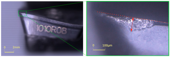
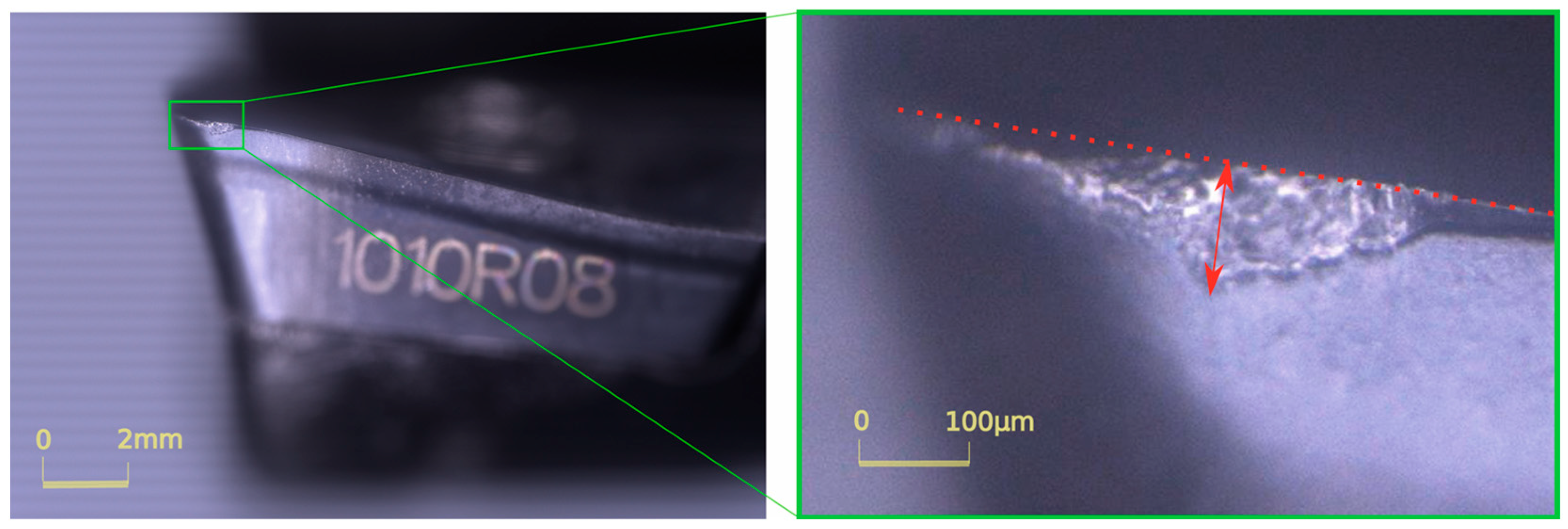
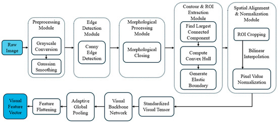
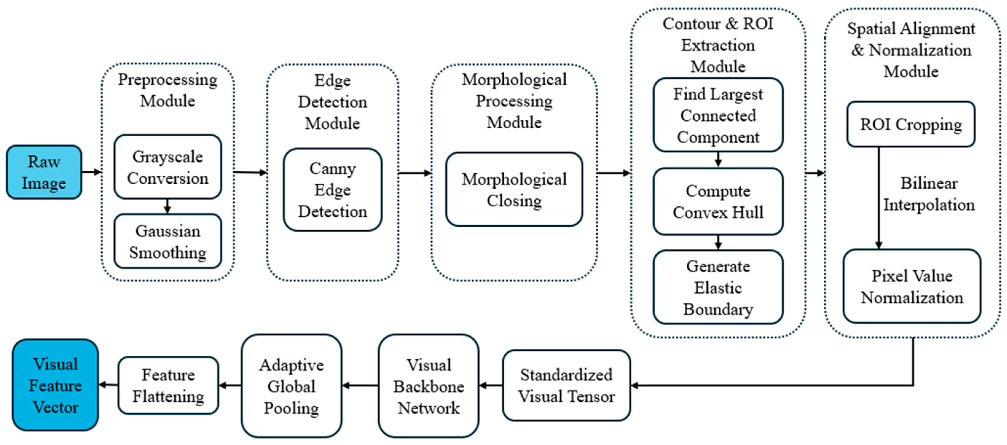
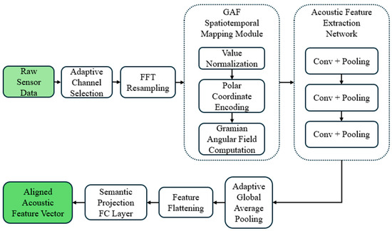
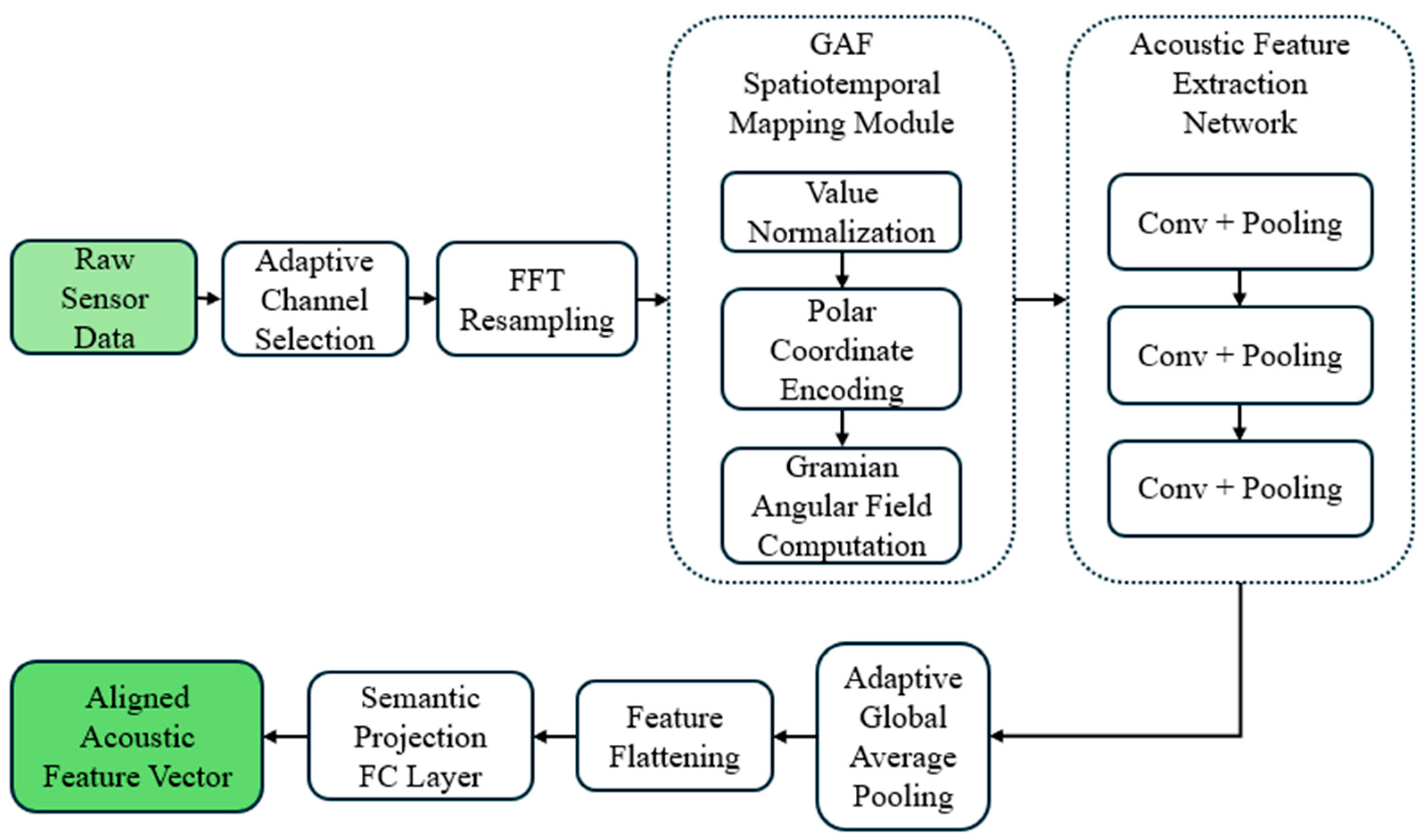
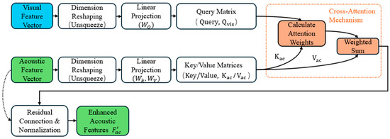
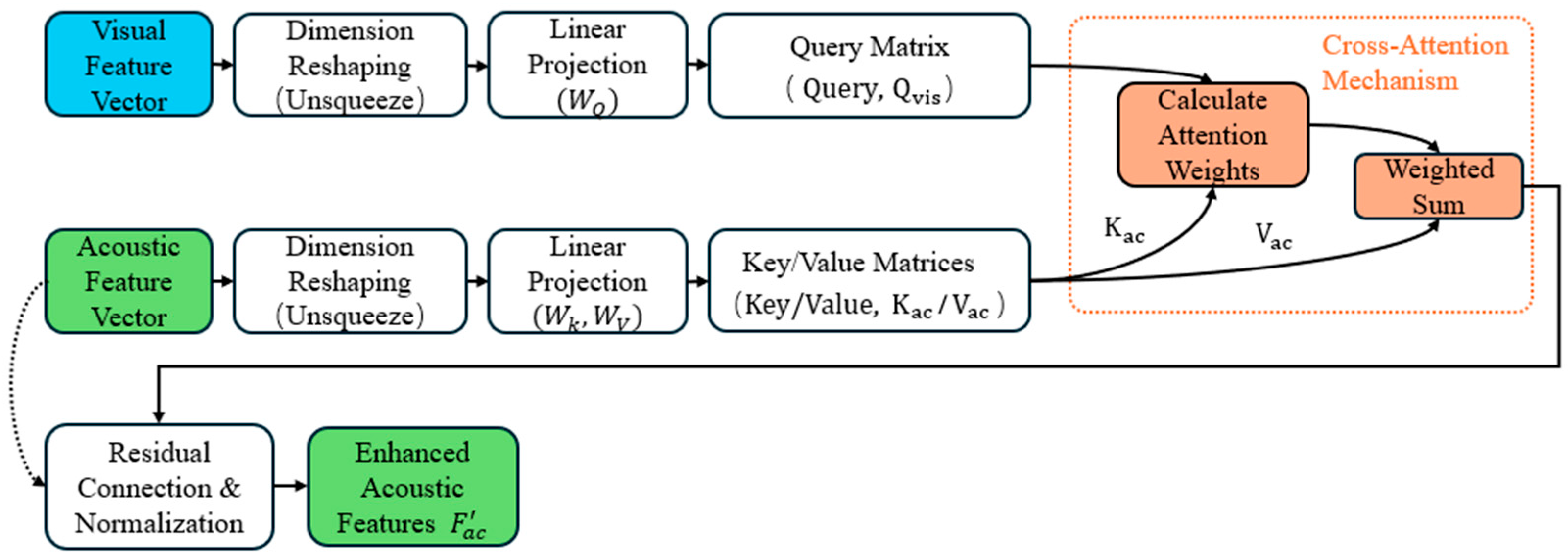
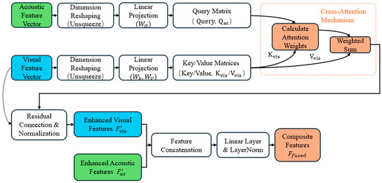
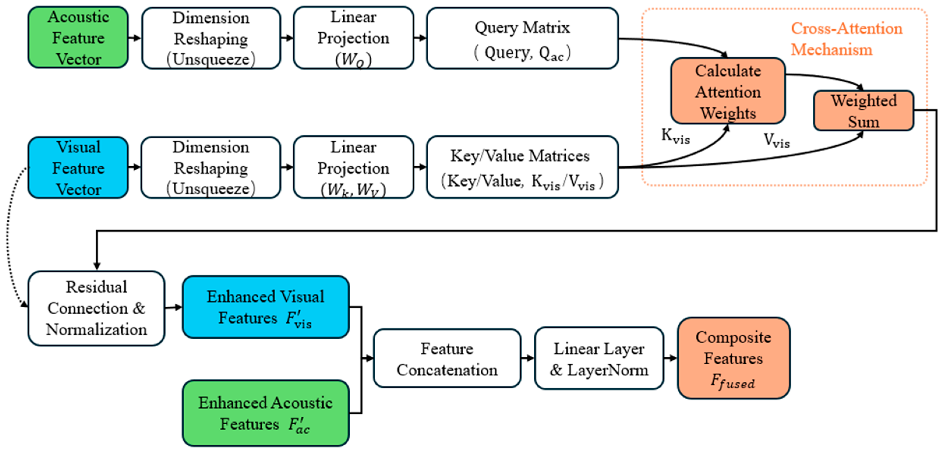
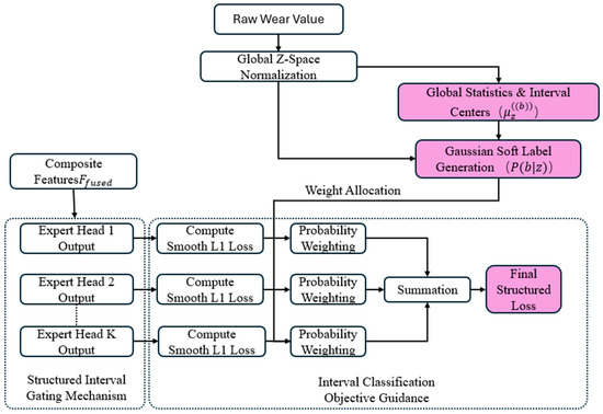
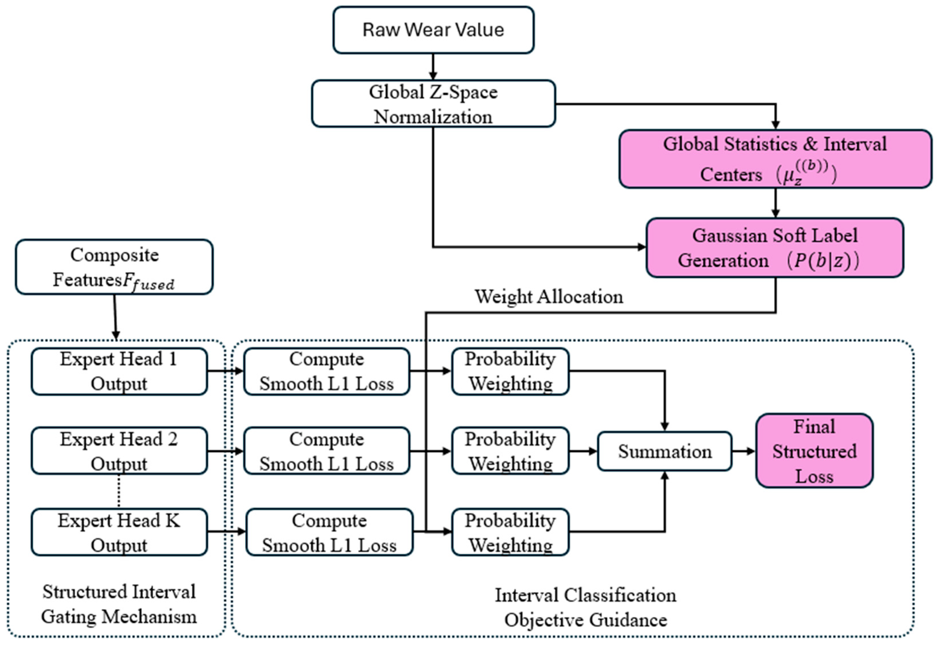
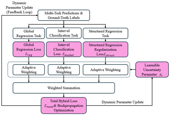
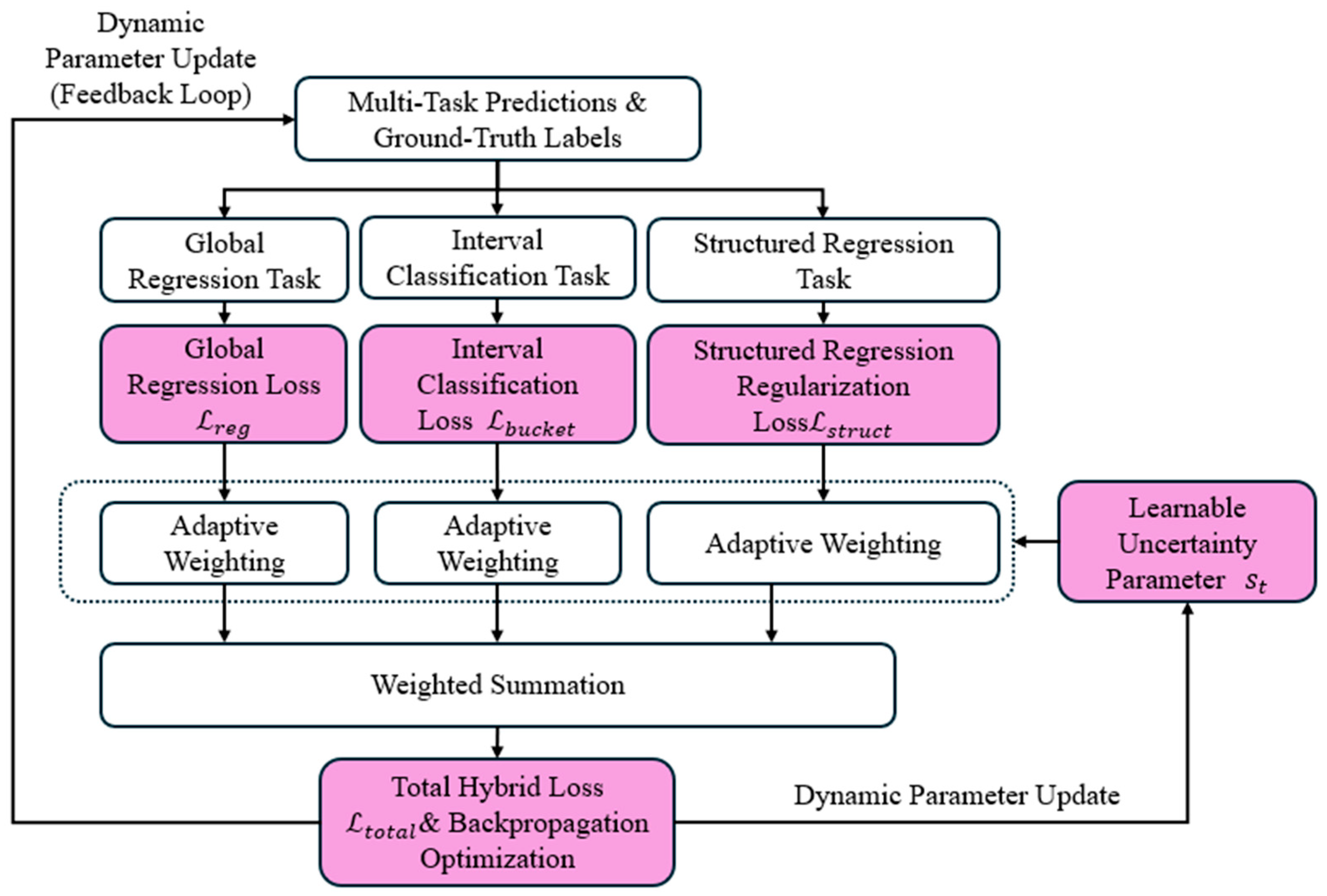
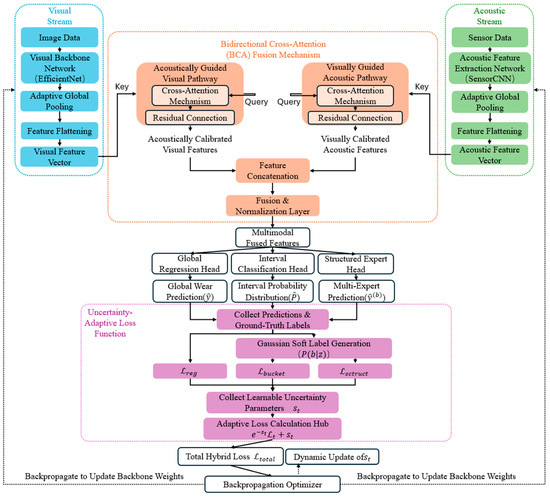
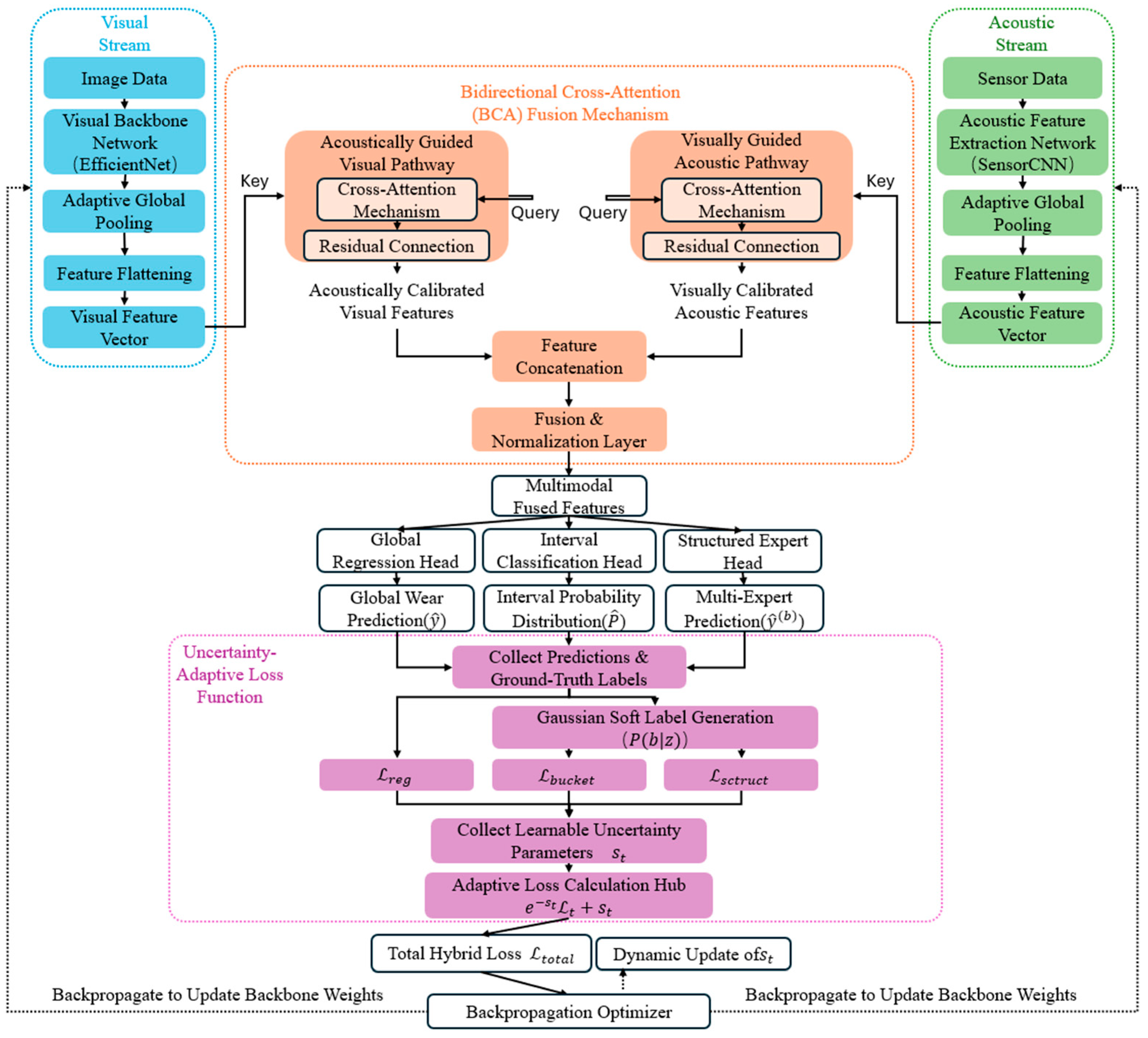
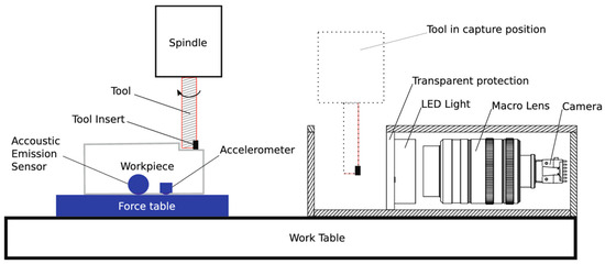
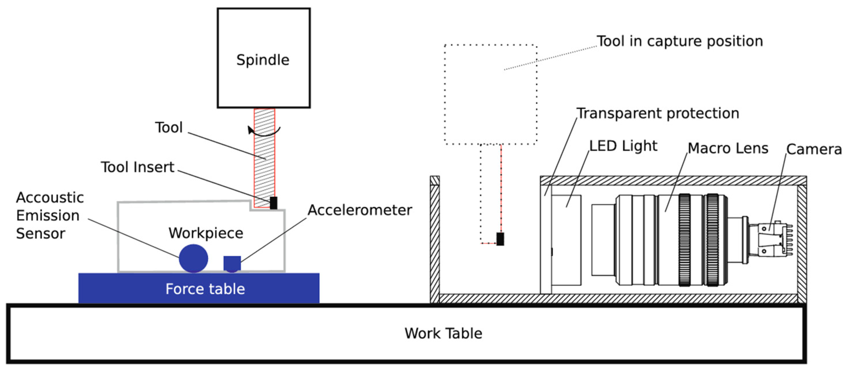
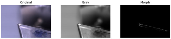
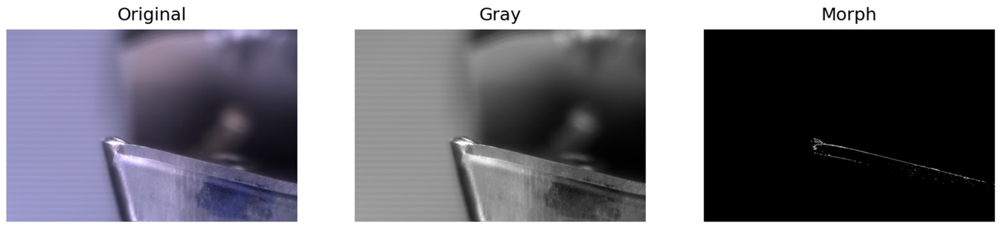
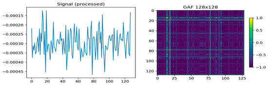
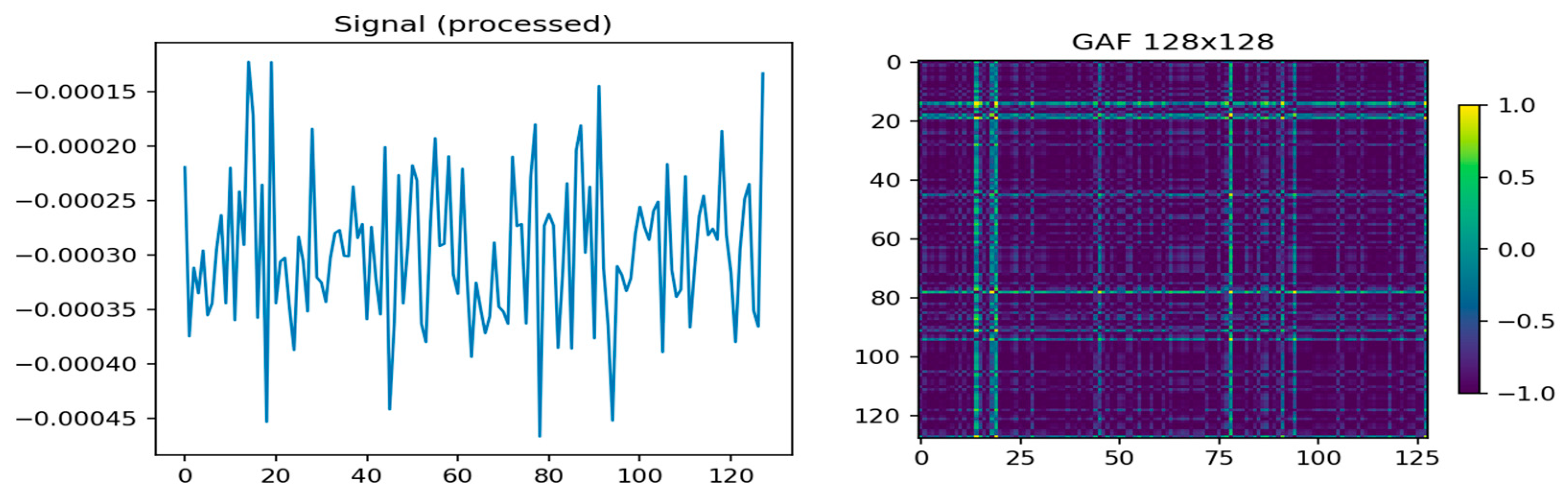
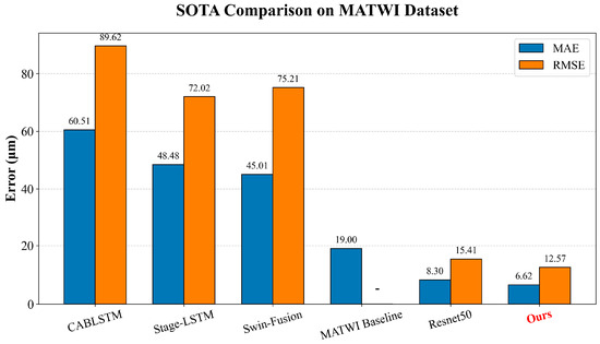
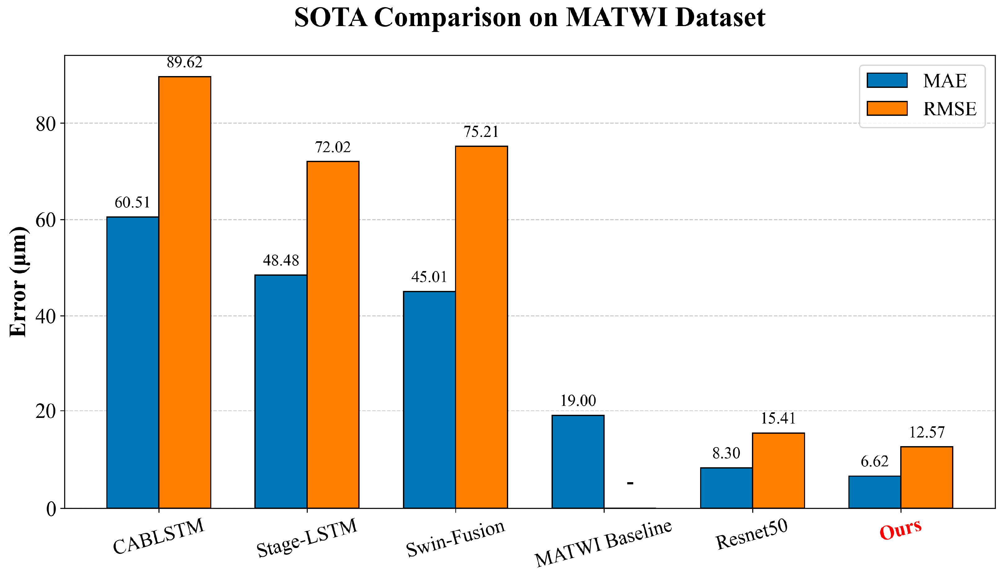
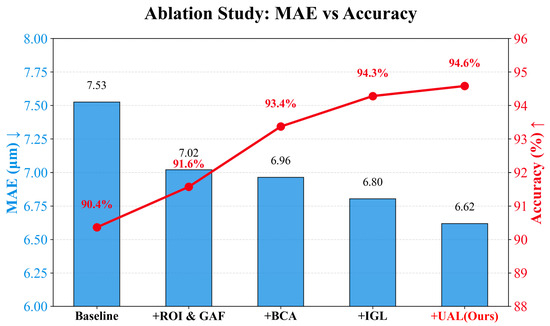
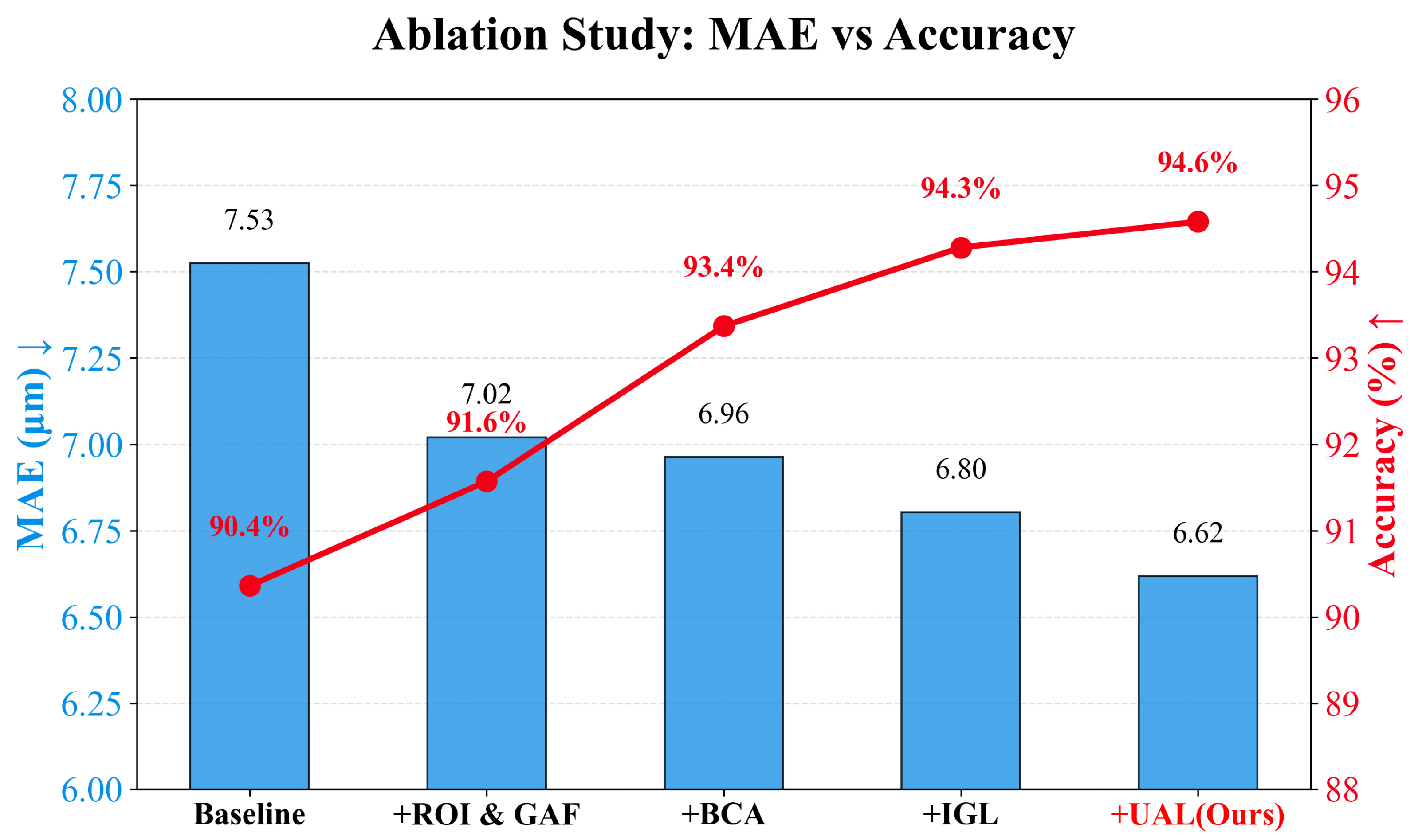
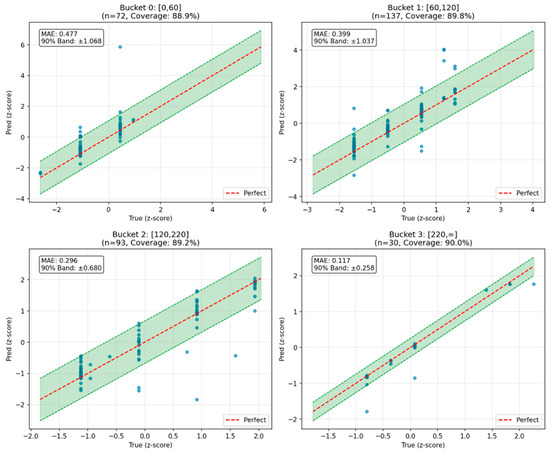
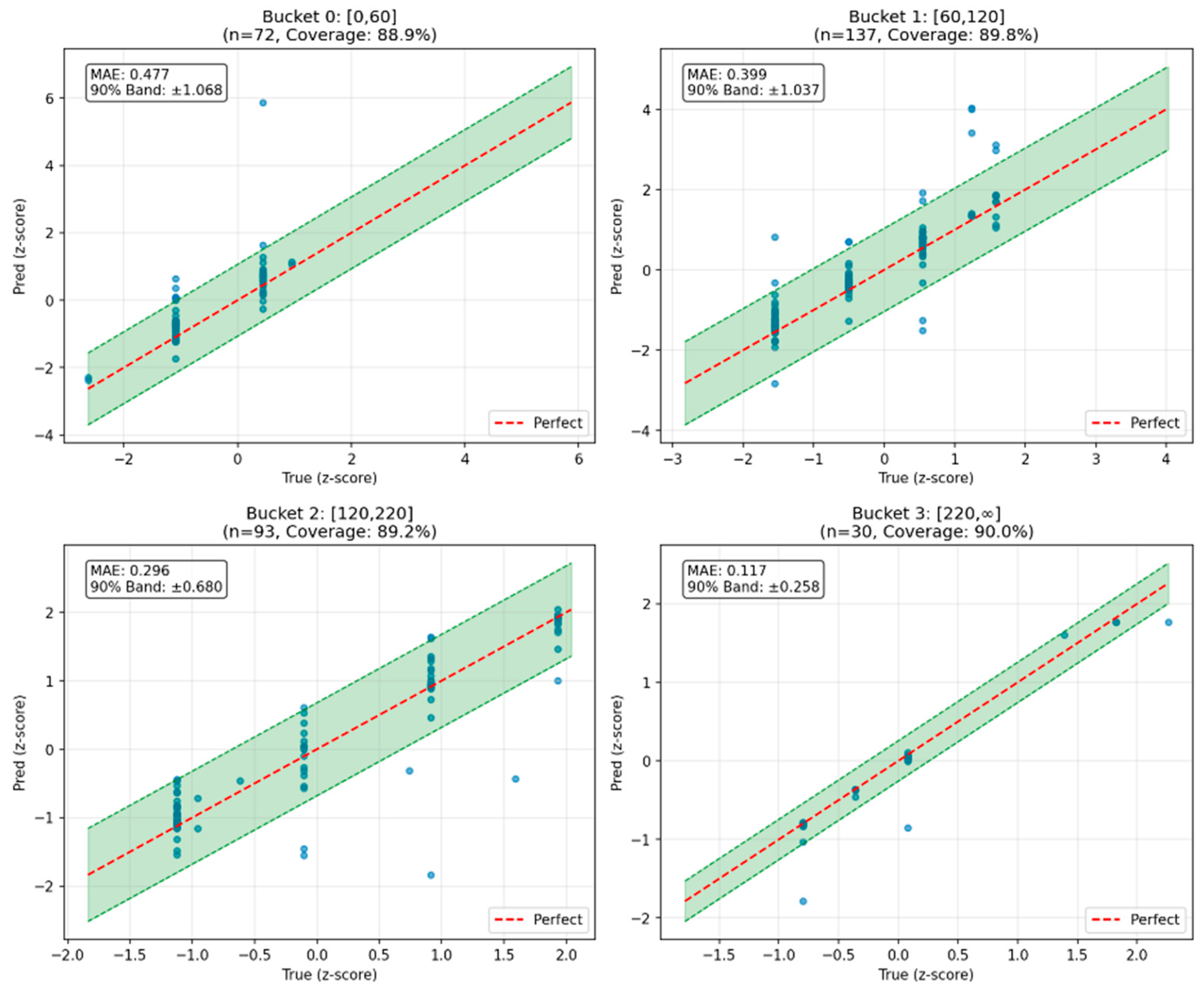

Disclaimer/Publisher’s Note: The statements, opinions and data contained in all publications are solely those of the individual author(s) and contributor(s) and not of MDPI and/or the editor(s). MDPI and/or the editor(s) disclaim responsibility for any injury to people or property resulting from any ideas, methods, instructions or products referred to in the content. |
© 2026 by the authors. Licensee MDPI, Basel, Switzerland. This article is an open access article distributed under the terms and conditions of the Creative Commons Attribution (CC BY) license.