


Abstract
Phase resistance unbalance in robotic joint drive systems can alter electromagnetic torque generation and degrade motion accuracy, but its early diagnosis is challenging because fault-related signatures are weak and coupled with operating dynamics. This study proposes a short-time Fourier transform (STFT)-based multi-scale attention ResNet for phase resistance-unbalance diagnosis using synchronized multi-sensor signals from a single industrial robotic joint. Controlled resistance-unbalance states were generated on an eRob70F100I-BM-18EN joint module by inserting 0.05 and 0.1 series resistors into one motor phase with a nominal single-phase resistance of 0.75 . Current, acceleration, rotational speed, and torque signals were segmented and converted into four-channel STFT log-amplitude maps. A modified ResNet18 backbone was integrated with feature pyramid network (FPN)-style multi-scale fusion and a convolutional block attention module (CBAM) to enhance discriminative time–frequency features. Under a window-level stratified split, the proposed model achieved 98.97% accuracy and 98.97% macro-F1, outperforming raw-signal, fast Fourier transform (FFT), wavelet, STFT-ResNet18, STFT-VGG11-BN, STFT-MobileNetV2, and STFT-ShuffleNetV2 baselines. Grouped validation was conducted using file-level, leave-one-speed-out, and leave-one-load-out splits to assess robustness under stricter data partitions. The proposed model achieved 91.75% macro-F1 under file-level splitting and average macro-F1 values of 89.77% and 84.22% under leave-one-speed-out and leave-one-load-out validation, respectively. Grad-CAM visualization further indicates that the model relies on non-uniform local time–frequency regions rather than uniformly using the entire spectrogram. These results demonstrate effective robotic-joint resistance-unbalance discrimination while revealing that unseen operating conditions, especially specific speed and load settings, remain challenging for robust cross-condition deployment.
1. Introduction
Industrial robots have become key equipment in modern manufacturing systems and are widely used in welding, handling, assembly, inspection, and other production tasks. Compared with standalone rotating machinery, an industrial robot is a coupled system composed of joint actuators, reducers, link structures, and control loops. A fault in a joint drive may propagate through the actuator, transmission mechanism, controller, and task-level motion, thereby affecting motion accuracy, dynamic response, production rhythm, and operational safety. Condition monitoring and fault diagnosis of industrial robots are therefore shifting from scheduled maintenance toward condition-based maintenance. However, robot diagnosis remains challenging because of multi-axis coupling, time-varying posture, variable payload, non-stationary motion, and the scarcity of fault data. Developing an effective fault diagnosis method for robotic joint drive systems is thus of practical engineering significance.
The specific fault investigated in this study is phase resistance unbalance in a robotic joint drive system. In a three-phase permanent-magnet synchronous motor drive, loose terminals, contact degradation, connection deterioration, or local winding-related abnormalities may introduce additional resistance and cause asymmetric phase impedance. Existing studies on resistive unbalance and high-resistance connection faults in permanent-magnet synchronous motor systems have shown that such electrical asymmetry can lead to current unbalance, increased copper loss and heat generation, torque ripple, efficiency reduction, and premature aging [1,2,3,4]. In a robotic joint drive system, such an electrical-side abnormality may not be reflected only in the current waveform. Through electromechanical coupling, it may also affect torque output, RPM-related signal characteristics, and vibration responses. Therefore, resistance-unbalance diagnosis in robotic joint drive systems requires both an electrical-fault perspective and a signal representation suitable for non-stationary joint operation data.
Mechanistically, this fault is different from common mechanical faults in robot joints, such as bearing defects, reducer wear, joint looseness, or backlash-related faults. Mechanical faults usually originate from the transmission or structural side and first manifest as local impact, stiffness variation, friction change, or vibration modulation. In contrast, phase resistance unbalance originates from phase-impedance asymmetry on the electrical side. The additional phase resistance changes the phase voltage–current relationship, distorts the three-phase current distribution, and consequently perturbs electromagnetic torque generation. The resulting torque ripple then acts as an internal excitation that is transmitted through the motor–reducer–load chain and is reflected in speed-related, torque, and vibration responses with different transmission paths and sensitivities. This electromechanical-coupling mechanism motivates the use of current as the primary diagnostic signal and the systematic evaluation of RPM-related, torque, and acceleration channels as auxiliary responses.
Existing robot fault diagnosis studies provide useful foundations, but they have not sufficiently addressed the above specific problem. Model-driven methods, such as observer-based and prediction-error-based diagnosis, construct residuals by comparing measured responses with robot dynamic or kinematic models and provide good physical interpretability [5,6]. These methods can be effective when the model, parameters, and measured states are reliable. In practical joint drive systems, however, friction, transmission dynamics, payload variation, backlash, controller action, and measurement noise make robust residual design difficult under variable operating conditions. Data-driven methods reduce the dependence on explicit analytical models and have become an important route for robot fault diagnosis. Early or shallow neural-network methods usually rely on posture, trajectory, or statistical features for classification. For example, Zhang and Zhu developed a BP-neural-network diagnostic model based on the end-effector position and attitude trajectory of a manipulator [7], and Hu also applied a BP neural network to robot-joint fault diagnosis [8]. These approaches are lightweight and easy to implement, but their performance depends heavily on manually constructed kinematic or statistical features, and their ability to learn complex electromechanical coupling responses in an end-to-end manner is limited.
Deep learning methods further improve automatic feature extraction. Pan et al. applied deep convolutional networks to robot-joint sensor and actuator fault diagnosis and further used deep residual networks to identify gain errors, bias faults, and failure faults [9,10]. Adam et al. constructed a two-dimensional CNN diagnostic model for an industrial robot test-bench dataset [11]. Yang et al. investigated ball-screw fault diagnosis in industrial robots using non-stationary motor-current signals [12]. These studies demonstrate the feasibility of DCNN, ResNet, and two-dimensional CNN models in robot-related diagnosis. Nevertheless, most of them focus on sensor or actuator signal faults, mechanical transmission faults, or test-bench fault categories. The multi-channel electromechanical responses induced by phase resistance unbalance in a single-joint robotic drive system remain insufficiently discussed.
From the viewpoint of the input form, one-dimensional deep networks that directly process raw time-domain signals are also common in mechanical fault diagnosis. A 1D-CNN can learn local patterns from raw signals in an end-to-end manner [13], while WDCNN uses a wide first-layer convolution kernel to enhance feature extraction from raw vibration signals [14]. For robot drive control systems, Wang et al. adopted a CNN-LSTM observer, in which the CNN extracts dynamic features, and the LSTM performs time-series prediction for fault detection in the motor drive control system of industrial robots [15]. These time-domain models have short input pipelines and a high degree of automatic feature learning. However, raw windows do not explicitly expose local frequency structures. If fault information appears as non-stationary time-frequency patterns, the network must implicitly learn frequency responses from the waveform, which may increase training difficulty. Therefore, this paper includes 1D-CNN, WDCNN, and CNN-BiLSTM as raw time-domain deep-learning baselines in the cross-model comparison.
For non-stationary diagnostic signals, time-frequency analysis and multiresolution signal processing have been widely used. Wavelet analysis provides localized multiscale decomposition and has been applied to industrial robot bearing and joint-related fault diagnosis [16,17,18]. Other studies have organized industrial-robot or rotating-machinery signals into two-dimensional representations before inputting them into convolutional networks, enabling neural networks to learn local patterns that are difficult to describe using scalar handcrafted features [11,19]. Nevertheless, signal representation remains a critical design choice. Raw signals preserve temporal details but do not explicitly show frequency structures; FFT spectra describe global frequency components but lose local temporal variation; wavelet representations provide multiscale localization but depend on the selected wavelet basis and scale construction; and STFT spectrograms provide a direct and controllable time-frequency representation through a sliding analysis window. Therefore, this study systematically compares raw signal, FFT, wavelet, and STFT representations under the same training protocol and selects STFT as the final input representation according to the empirical results on the present dataset.
When learning from STFT maps, convolutional neural networks are suitable because spectrograms contain local time-frequency patterns. Residual learning alleviates degradation in deep convolutional feature extraction and has been widely used as a backbone for image-like diagnostic inputs [20,21]. In addition, attention and multimodal fusion have been used to improve feature selection and information fusion in industrial robot fault diagnosis. Lu et al. proposed a dual-module attention CNN for industrial robot reducer fault diagnosis to capture different types of fault-related features [22]. Zhou et al. proposed an attention-enhanced multimodal deep-learning method for multi-source feature extraction and fusion in robotic compound fault diagnosis [23]. These studies indicate that attention and multi-source information fusion are valuable for robot fault diagnosis. However, existing methods are mainly oriented toward the reducer or compound mechanical faults, and some model structures are relatively complex. The aim of this paper is not to expand network capacity, but to construct a compact and reproducible diagnostic framework under a small-sample dataset with explicit physical prior knowledge. Therefore, STFT-ResNet18 and STFT-VGG11-BN are selected as two-dimensional CNN baselines, and the final model combines feature-pyramid-style multi-scale feature fusion with the convolutional block attention module (CBAM). Feature pyramid networks were originally proposed to fuse high-level semantic features and low-level spatial features through a top-down pathway [24]; CBAM sequentially infers channel and spatial attention maps and has a compact structure suitable for convolutional backbones [25]. Based on these considerations, this paper adopts an STFT-ResNet18-FPN/MSF-CBAM architecture.
Based on the above analysis, this study addresses three main research gaps. First, compared with existing robot diagnosis studies on mechanical faults, sensor faults, actuator faults, or whole-system test-bench faults, phase resistance unbalance in a single-joint robotic drive system lacks targeted investigation. Second, although current signals are physically related to resistance unbalance, the value of acceleration, RPM-related, and torque signals as auxiliary inputs for this robotic-joint task requires systematic verification. Third, under small-sample conditions with explicit physical prior knowledge, the selection of an effective signal representation and a compact deep network structure requires empirical analysis. To address these issues, this study constructs a four-channel robotic-joint small-sample dataset with physical prior knowledge, compares multiple signal representations and representative deep-learning diagnostic models, proposes an STFT-ResNet18-FPN/MSF-CBAM diagnostic model, and evaluates model components, sensor-channel contributions, grouped validation behavior, and deployment-oriented model complexity. The overall diagnostic workflow is shown in Figure 1.
Figure 1.
Overall workflow of the proposed phase resistance unbalance diagnosis method for a robotic joint drive system. Blue, green, purple, orange, and red identify the five processing stages; in the output panel, green, amber, and red denote the Normal, Unbalance_0.05R, and Unbalance_0.1R classes, respectively.
The main experiments use a window-level stratified split to evaluate within-dataset discrimination under a unified data protocol. File-level, leave-one-speed-out, and leave-one-load-out grouped-validation settings are also included to assess whether the learned features remain effective under stricter data partitions. Under this scope, the main contributions of this work are summarized as follows:
- A small-sample experimental dataset with physical prior knowledge is constructed for phase resistance unbalance diagnosis in a single-joint industrial robotic drive system. The experiment simulates different degrees of phase resistance unbalance by inserting 0.05 and 0.1 series resistors into one motor phase with a nominal single-phase resistance of approximately 0.75 , corresponding to relative resistance increments of 6.67% and 13.33%, respectively.
- A four-channel synchronized sample construction procedure is established using acceleration, current, RPM-related, and torque signals. Current is used as the primary electrical diagnostic baseline, and the marginal contributions of the auxiliary sensor channels are systematically analyzed from both performance and electromechanical coupling perspectives.
- Raw signal, FFT, wavelet, and STFT representations are compared under a unified training protocol. The results verify that STFT log-amplitude maps are more suitable as the input representation for the robotic joint phase resistance-unbalance task considered in this paper.
- An STFT-ResNet18-FPN/MSF-CBAM single-task classification network is proposed by combining residual convolutional feature extraction, FPN-style multi-scale feature fusion, and CBAM channel-spatial attention for learning fault-related discriminative features from multi-channel STFT maps. The proposed model is compared with representative one-dimensional time-domain models, two-dimensional time-frequency CNN models, and lightweight STFT-MobileNetV2/STFT-ShuffleNetV2 baselines.
- In addition to the main window-level evaluation, file-level and cross-condition grouped validation is conducted to examine generalization under unseen recording files, speeds, and loads. Model complexity, CNN MACs, end-to-end latency, and Grad-CAM visualization are further analyzed to clarify the performance–complexity trade-off and the qualitative interpretability of the proposed method.
The remainder of this paper is organized as follows. Section 2 presents the signal representation procedure and the proposed STFT-ResNet18-FPN/MSF-CBAM model. Section 3 describes the experimental platform, phase resistance unbalance fault injection, and dataset construction. Section 4 gives the experimental protocol and evaluation metrics. Section 5 reports and discusses the experimental results. Finally, Section 6 concludes the paper.
2. Signal Representation and Proposed Method
This section presents the proposed diagnosis method for robotic joint phase resistance unbalance. The method does not rely on a single deep-learning module alone. Instead, it integrates synchronized multi-channel acquisition, non-overlapping window segmentation, STFT time-frequency representation, hierarchical feature extraction using ResNet18, FPN-style multi-scale fusion, and CBAM attention enhancement into an end-to-end three-class diagnostic procedure.
For clarity, the method can be summarized in three steps:
- Four-channel synchronized signal windowing. Acceleration, current, RPM-related, and torque signals are segmented into 2048-point non-overlapping windows to obtain time-aligned multi-channel samples.
- STFT time-frequency representation. The STFT is computed for each channel. The log-amplitude spectra are then stacked along the channel dimension to form a model input of size .
- Deep feature learning and fault classification. The four-channel STFT input is fed into the STFT-ResNet18-FPN/MSF-CBAM network. ResNet18 extracts hierarchical features, the FPN-style module fuses multi-scale features, CBAM enhances key features, and the classification head outputs three fault-state logits.
2.1. Window Segmentation and Sample Construction
Let a raw four-channel signal be denoted as , where the four channels correspond to acceleration, current, RPM-related signal, and torque, respectively. A window-level sample construction method is adopted by dividing the continuous signal into fixed-length short-time segments. The k-th sample window is written as
Here, k is the window index, n is the sample index inside the window, c is the channel index, and is the window length. Therefore, a single window sample satisfies . Non-overlapping windows are used, so the window step is also 2048 sampling points. Given the sampling frequency of 25 kHz, each window corresponds to s, i.e., 81.92 ms.
The window length must balance local temporal structure, frequency resolution, sample number, and local stationarity. A window length of 2048 samples is selected because it corresponds to 81.92 ms at 25 kHz, provides sufficient local temporal coverage and a manageable STFT computational scale, and avoids excessive smoothing of short-time disturbances by overly long windows. This parameter is used as a fixed preprocessing setting in the unified experimental protocol.
Figure 2 shows the non-overlapping segmentation of the four-channel synchronized signals. The four channels remain time-aligned within each window. Therefore, a sample contains not only the electrical-side response in the current signal, but also electromechanical response information from the acceleration, RPM-related, and torque signals.
Figure 2.
Non-overlapping window segmentation of four-channel synchronized signals.
2.2. Overall Framework of the Proposed Method
After window segmentation, the STFT-ResNet18-FPN/MSF-CBAM network is constructed for three-class fault diagnosis. The overall architecture is shown in Figure 3. The model first receives a time-frequency input of size , where B denotes the batch size. The input is then processed by a modified ResNet18 backbone to extract hierarchical features. FPN-style top-down fusion is used for multi-scale feature fusion. CBAM is then applied to enhance the channel and spatial responses of the fused features. Finally, global average pooling, dropout, and a fully connected layer generate three-class logits. During inference, the logits can be converted to class probabilities using softmax.
Figure 3.
Architecture of the STFT-ResNet18-FPN/MSF-CBAM network. Ellipses denote repeated per-channel inputs or feature maps and do not indicate omitted processing stages.
The design motivation is as follows. STFT maps explicitly represent local frequency structures. ResNet18 extracts hierarchical features ranging from low-level local textures to high-level semantic patterns. FPN-style fusion allows the model to use features at different resolutions, and CBAM further emphasizes fault-related channels and time-frequency regions.
2.3. STFT-Based Time-Frequency Representation
The short-time Fourier transform (STFT) uses a finite-length analysis window that slides along the time axis and computes the Fourier transform for each local time segment. Therefore, STFT can describe signal temporal locality and frequency structure simultaneously to some extent. For robotic joint operation signals, load, speed, and electrical abnormalities may cause local non-stationary changes. STFT is therefore more suitable than a global FFT for describing such short-time local frequency variations.
For the c-th sensor channel, a Hann window is used to compute the STFT of the signal within each window. Let the analysis-window length be , the frame shift be H, and the FFT length be . The STFT is defined as
Here, c denotes the sensor-channel index, k and m denote the frequency-bin and time-frame indices, respectively, is the Hann window function, and denotes the reflected-padded signal of the c-th channel because center=True and pad_mode=reflect are used. The STFT parameters are n_fft=256, win_length=256, hop_length=16, and onesided=True. To reduce the magnitude dynamic range and enhance spectrogram readability, a logarithmic transform is applied to the STFT magnitude:
The log-amplitude spectra of the four channels are stacked along the channel dimension to form a four-channel time-frequency input tensor:
In the implementation, the computed STFT log-amplitude spectra of each channel are adjusted to a fixed size of to satisfy the network input requirement.
Figure 4 shows examples of current-channel STFT maps for the three phase-resistance states under the same operating condition. Because phase resistance unbalance first affects the electrical side, the time-frequency distribution of the current channel can intuitively reflect local spectral-energy differences under different fault severities.
Figure 4.
Current-channel STFT examples for three phase-resistance states under the same operating condition. The color scale represents , with dark purple indicating lower log-amplitude and yellow–red indicating higher log-amplitude.
Under multi-sensor input, the four channels are not simply concatenated into a one-dimensional sequence. Instead, each channel is transformed into a log-amplitude STFT map, and the four maps are stacked along the channel dimension to form a four-channel time-frequency tensor. Figure 5 illustrates the construction process of the four-channel STFT input tensor.
Figure 5.
Construction of the four-channel STFT input tensor.
The STFT parameters were selected to balance time resolution, frequency resolution, and input consistency for the CNN backbone. The frame length and FFT size were both set to 256 samples. At the sampling frequency of 25 kHz, this setting corresponds to a frame duration of 10.24 ms and a frequency-bin spacing of approximately 97.66 Hz, which provides local frequency information while preserving short-time variations in the measured signals. The hop length was set to 16 samples to obtain a dense time-frequency representation and improve the continuity of local spectral patterns. A Hann window was used to reduce spectral leakage caused by short-time truncation. The log-amplitude mapping was applied to compress the spectral dynamic range and reduce the dominance of high-energy components. Finally, the STFT maps were resized to to provide a fixed-size input for the CNN backbone. The same STFT settings were used for all STFT-based models to ensure fair comparison.
The STFT representation and model-input parameters are summarized in Table 1.
Table 1.
STFT representation and model-input parameters.
2.4. Residual Feature Extraction
ResNet18 is used as the backbone feature extractor in this study. The core idea of ResNet is residual learning, in which the network learns a residual function rather than the complete mapping from input to output. For a residual block, the output can be expressed as
Here, is the input feature, denotes the residual mapping composed of convolution, normalization, and nonlinear activation, and denotes learnable parameters. When the input and output channel numbers or spatial sizes are inconsistent, a projection shortcut can be used to match the input:
Residual connections help alleviate degradation during the training of deep networks and enable multi-level feature extraction. For the STFT-map input in this paper, shallow features help capture local spectral lines and short-time energy variations, whereas deeper features help form more abstract fault-discriminative patterns. Because the input contains four-channel time-frequency maps, the first convolutional layer of ResNet18 is modified to accept four input channels.
2.5. FPN-Style Multi-Scale Feature Fusion
Phase resistance unbalance in a robotic joint may appear at different scales in the time-frequency map. Local frequency-band energy changes, short-time speed-related variations, and cross-band coupling patterns may coexist. Using only a single level of deep features may ignore shallow details, whereas relying only on shallow features may not provide sufficient class-discriminative capability. Therefore, an FPN-style multi-scale fusion (MSF) module is introduced after the ResNet18 backbone.
As shown in the lower FPN detail region of Figure 3, the output features of layer2, layer3, and layer4 in ResNet18 are used and denoted as , , and , respectively. The FPN module first maps features at different levels to 256 channels using lateral convolutions and then performs stepwise fusion through a top-down pathway:
Here, denotes a lateral convolution, and denotes upsampling. , , and represent multi-scale features after top-down fusion rather than the original lateral features. The final fused feature is aligned to the scale and used for subsequent attention enhancement and classification.
2.6. CBAM Attention Enhancement and Classification Output
To further emphasize fault-related channels and time-frequency regions, the convolutional block attention module (CBAM) is introduced after multi-scale fusion. CBAM sequentially contains channel attention and spatial attention. Channel attention evaluates the importance of different feature channels, while spatial attention highlights local regions in the time-frequency map that are more diagnostically informative.
Let the fused input feature be . Channel attention is computed by applying global average pooling and max pooling along the spatial dimensions, passing both descriptors through a shared MLP, summing the outputs, and applying a sigmoid function:
The feature after channel attention is
Spatial attention is then computed by applying average pooling and max pooling along the channel dimension, concatenating the two maps, and passing them through a convolution and a sigmoid function:
The final enhanced feature is
Here, ⊗ denotes element-wise multiplication. Through this sequential attention mechanism, the model can automatically enhance feature responses related to phase resistance unbalance while suppressing redundant or weakly related regions during end-to-end training.
The enhanced feature output by CBAM passes through global average pooling, dropout, and a fully connected layer to obtain three-class logits. The task is formulated as a single-task three-class classification problem with the classes Normal, Unbalance_0.05R, and Unbalance_0.1R.
3. Experimental Platform and Small-Sample Dataset with Physical Prior Knowledge
3.1. Robotic Joint Drive Experimental Platform
A self-built single-joint robotic drive experimental platform was used to conduct the phase resistance unbalance diagnosis experiments. The experimental object was an eRob70F100I-BM-18EN robotic joint module. The eRob series joint module integrates a servo drive, absolute encoder, frameless torque motor, brake, precision harmonic reducer, and related components, making it suitable for constructing a compact robotic joint drive unit.
The experimental platform mainly consists of the robotic joint module, output flange, swing-arm load, external torque sensor, acceleration sensor, current sensor, and a robotic joint data acquisition system (RJDA system). The joint module outputs torque through the motor and reducer and drives the swing arm under specified speed and load conditions. The external torque sensor is installed between the joint output end and the swing arm to acquire the output torque response.
Figure 6 shows the experimental bench, the phase resistance-unbalance fault-injection position, and the sensor arrangement.
Figure 6.
Experimental platform of the robotic joint drive system: (a) overall view of the experimental bench; (b) phase resistance-unbalance fault injection in one motor phase; (c) sensor arrangement for acceleration, current, torque, RPM-related, and acquisition-system signals.
3.2. Phase Resistance-Unbalance Fault Injection
The fault type considered in this paper is phase resistance unbalance in the robotic joint drive system. This fault is used to simulate electrical-side asymmetry caused by increased motor phase-connection resistance, terminal contact degradation, wiring looseness, or local winding resistance abnormalities. Phase resistance unbalance breaks the impedance symmetry of the three-phase winding, changes the amplitude and phase relationship of the phase currents, and may further cause torque fluctuation, increased heat generation, reduced efficiency, and abnormal joint operation.
To construct controllable phase resistance-unbalance states, an external resistor was connected in series with one motor phase. The nominal single-phase resistance of the motor was approximately before external fault injection. Three states were considered: Normal, Unbalance_0.05R, and Unbalance_0.1R. Normal denotes the healthy state without an external series resistor. Unbalance_0.05R denotes a mild phase resistance-unbalance state generated by inserting a resistor into one phase, corresponding to a relative increment of approximately with respect to the nominal phase resistance. Unbalance_0.1R denotes a higher phase resistance-unbalance state generated by inserting a resistor into one phase, corresponding to a relative increment of approximately . This fault injection strategy is a controlled experimental simulation designed to construct a labeled dataset with distinguishable fault severities.
It should be clarified that the external series-resistor setting is not equivalent to all possible high-resistance connection faults in real industrial fields. It is a controllable simulation of the phase resistance-unbalance phenomenon. This setting enables repeatable and labeled fault data to be obtained without damaging the robotic joint module itself.
3.3. Synchronized Multi-Sensor Data Acquisition
To characterize the operating responses of the robotic joint drive system under different electrical states, four signal channels were synchronously acquired. CH1 is the acceleration signal, CH2 is the current signal, CH3 is the RPM-related signal provided by the torque-sensor unit, and CH4 is the torque signal. Because phase resistance unbalance first appears as electrical-side asymmetry, the current signal is regarded as the primary diagnostic baseline. Acceleration, RPM-related, and torque signals are used to evaluate whether electromechanical coupling responses provide additional diagnostic information.
The sampling frequency was , and each recording lasted . The four channels were synchronously acquired by the RJDA system and remained time-aligned during subsequent window segmentation and time-frequency transformation. Figure 7 illustrates the phase resistance-unbalance fault injection and synchronized multi-sensor data acquisition procedure.
Figure 7.
Schematic of phase resistance-unbalance fault injection and synchronized multi-sensor data acquisition. Red lines indicate the inserted series-resistance path, the red/green/yellow lines denote the three motor-phase connections, and black lines indicate signal connections to the RJDA system. CH1–CH4 correspond to acceleration, current, RPM-related, and torque signals, respectively.
The channel definitions, sensitivities, and measured responses are summarized in Table 2.
Table 2.
Description of the multi-sensor acquisition channels.
3.4. Dataset Construction
After data acquisition, the continuous raw signals were divided into non-overlapping windows. The window length was set to 2048 sampling points, and the step size was also set to 2048 sampling points. With a sampling frequency of , the time duration of each window is
Thus, each window covers approximately of joint operation. Each window contains four synchronized channels, so the raw input sample can be represented as .
The experimental data cover three fault states, five load conditions, and three rotational-speed conditions. The load conditions are 0, 1, 2, 3, and 4 kg, and the rotational-speed conditions are 5, 10, and 20 rpm. Therefore, each fault category contains 15 operating-condition combinations. The dataset contains 65,880 window samples in total, with 21,960 samples for each class. The dataset was then divided into training, validation, and test sets using a window-level stratified random split with ratios of 70%, 15%, and 15%, corresponding to 46, 116, 9882, and 9882 samples, respectively.
The three fault classes, added resistances, relative resistance increments, and sample counts are summarized in Table 3.
Table 3.
Fault classes, added series resistances, and relative increments with respect to .
The main performance comparison adopts a window-level stratified random split to maintain a unified protocol across representation, model, ablation, and sensor-combination experiments. Because windows are generated from a limited number of original recording files, grouped-validation experiments are conducted in Section 5.6 to evaluate performance under file-level, speed-held-out, and load-held-out settings. This distinction is important for interpreting the difference between within-dataset discrimination and stricter cross-condition generalization.
3.5. Physical Prior Nature and Experimental Boundary
The dataset is described as a small-sample dataset with physical prior knowledge because its construction is guided by the known electromechanical effect of phase resistance unbalance. First, the fault injection is not arbitrary: the inserted resistors introduce controlled increments relative to the nominal phase resistance, thereby defining repeatable severity levels. Second, the selected channels reflect the expected fault-propagation path. Current is the primary electrical response, while the RPM-related and torque signals are associated with torque generation and joint dynamics, and acceleration provides a structural vibration response. A simplified rotational dynamic relationship can be written as
where J is the equivalent inertia, is the rotational speed, is the electromagnetic torque, is the load torque, B is the viscous coefficient, and denotes friction-related disturbance. Phase resistance unbalance perturbs the phase-current distribution and may introduce torque ripple; such torque disturbance can be reflected in speed-related and torque responses before being transmitted through the reducer, housing, and sensor-mounting path to the acceleration channel. Therefore, under the present fault type and sensor configuration, the RPM-related signal can be more directly coupled with the electrical-side disturbance than the acceleration response.
This physical-prior setting also defines the boundary of the study. The external series-resistor experiment simulates a controlled phase-resistance increase and does not reproduce all nonlinear, temperature-dependent, or intermittent behaviors of real poor-contact or high-resistance connection faults, such as waveform clipping and intermittent disconnection in severe poor-contact conditions.
Table 4 summarizes how the above physical prior knowledge is transformed into specific experimental and algorithmic decisions. The purpose of this mapping is to avoid treating the model as a purely data-driven black box and to clarify the reproducibility boundary of the proposed diagnostic framework.
Table 4.
Transformation of physical prior knowledge into experimental and algorithmic decisions.
4. Experimental Protocol and Evaluation Metrics
This section describes the data-splitting strategy, training settings, evaluation metrics, and comparative experiment design used in this study. To ensure comparability among different experiments, the same data split, random seed, training parameters, and model-selection criterion are maintained whenever possible, except for the factor under investigation.
The primary experiments evaluate the ability of the proposed STFT-ResNet18-FPN/MSF-CBAM method to recognize phase resistance unbalance states under a unified window-level data protocol. To address the risk that window-level splitting may overestimate generalization, grouped validation experiments are also designed at the file, rotational speed, and load-condition levels. Therefore, the experimental protocol contains both within-dataset evaluation and stricter grouped-validation tests.
4.1. Data-Splitting Protocol
The acquired window samples were randomly divided into training, validation, and test sets with ratios of 70%, 15%, and 15%, respectively, using stratification according to fault class. Stratified splitting ensures that the proportions of Normal, Unbalance_0.05R, and Unbalance_0.1R samples remain consistent across different subsets. All main experiments use the same random seed and the same data split to avoid incomparable results caused by different split partitions.
Under this splitting strategy, the dataset contains 65,880 window samples in total. The training set contains 46,116 samples, the validation set contains 9882 samples, and the test set contains 9882 samples. Since the three classes are balanced, each class contains 3294 samples in the test set.
Table 5 summarizes the dataset-splitting protocol and the role of each subset.
Table 5.
Dataset splitting protocol.
4.2. Training Settings
All deep-learning models are trained under a unified training protocol. Model selection is based on validation Macro-F1. During training, the checkpoint with the best validation Macro-F1 is saved and then used for final evaluation on the test set. This strategy reduces the overfitting risk associated with selecting a model only according to training loss.
The final main experiments do not use data augmentation, and model training is conducted as a single-task three-class classification problem. The training loss is focal loss with and label smoothing of 0.05.
For two-dimensional CNN models with STFT-image input, ImageNet pretrained weights are used for initialization, and the first convolutional layer is adapted to four-channel input. For one-dimensional time-domain models such as 1D-CNN, WDCNN, and CNN-BiLSTM, the network structures are incompatible with ImageNet image models; therefore, their parameters are trained from scratch. This setting is used to maintain fairness among models of the same type while reflecting the practical training strategy of using pretrained two-dimensional convolutional backbones under small-sample data conditions.
The complete model-training hyperparameters are reported in Table 6.
Table 6.
Model training hyperparameters.
4.3. Evaluation Metrics
Accuracy, Precision, Recall, F1-score, and Macro-F1 are used as the main evaluation metrics, together with confusion-matrix analysis to examine misclassification among classes. Because the three classes are balanced in this study, Accuracy reflects the overall classification correctness. Macro-F1 assigns equal weight to each class and avoids masking class-wise performance differences by using only an overall accuracy value.
For the i-th class, let , , and denote true positives, false positives, and false negatives, respectively. Precision, Recall, and F1-score are defined as
For K classes, Macro-F1 is defined as the arithmetic mean of class-wise F1-scores:
In this paper, . The final results report test-set Accuracy, Macro-Precision, Macro-Recall, Macro-F1, and the confusion matrix.
4.4. Comparative Experiment Design
To systematically verify the rationality of the design choices in the proposed method, four groups of comparative experiments are conducted: signal-representation comparison, representative deep-learning diagnostic model comparison, architecture ablation, and sensor-contribution analysis. Except for the factor being compared, all other experimental settings are kept consistent, including data split, random seed, training protocol, and model-selection criterion.
4.4.1. Signal-Representation Comparison
The first group of experiments verifies the necessity of the STFT representation. Raw signal, FFT, wavelet, and STFT representations are compared. This experiment answers whether an explicit time-frequency representation is more effective than raw time-series input, global spectra, or wavelet representation under the same data split and training conditions.
The settings and purpose of the signal-representation comparison are summarized in Table 7.
Table 7.
Settings for signal-representation comparison.
4.4.2. Representative Deep-Learning Diagnostic Model Comparison
The second group of experiments verifies the effectiveness of the proposed method relative to common deep-learning fault diagnosis models. The comparison includes one-dimensional deep models based on raw four-channel time-domain windows, lightweight STFT-based CNNs, general two-dimensional CNNs based on STFT-image input, and the proposed STFT-ResNet18-FPN/MSF-CBAM model. This experiment addresses three questions: whether STFT-image input outperforms direct time-domain modeling, how lightweight STFT backbones behave under the same input representation, and whether the proposed multi-scale fusion and attention-enhanced structure outperforms ordinary two-dimensional CNN baselines.
The compared models, inputs, pretraining settings, and purposes are listed in Table 8.
Table 8.
Settings for representative deep-learning diagnostic model comparison.
4.4.3. Architecture Ablation
The third group of experiments verifies the effectiveness of the FPN/MSF multi-scale fusion module and the CBAM attention module in the final model. Using STFT-ResNet18 as the base model, three variants are constructed by adding CBAM only, adding FPN/MSF only, and adding both FPN/MSF and CBAM. This experiment answers whether FPN/MSF and CBAM each improve the diagnostic performance of the basic ResNet18 and whether their combination provides complementary benefits.
The architecture-ablation settings are summarized in Table 9.
Table 9.
Settings for architecture ablation.
4.4.4. Sensor Contribution Analysis
The fourth group of experiments analyzes the marginal contribution of different sensor channels to diagnostic performance. Since phase resistance unbalance first appears as electrical-side asymmetry, the current channel is used as the primary baseline. Acceleration, RPM-related, and torque signals are then added to evaluate whether these auxiliary channels provide additional diagnostic information.
The eight sensor-combination settings and their purposes are listed in Table 10.
Table 10.
Settings for sensor-combination comparison.
4.5. Grouped-Validation Protocol
To examine whether the model performance is affected by the window-level split, three grouped-validation settings are used. First, a file-level split is used, in which all windows from the same original recording file are assigned exclusively to the training, validation, or test subset. This setting prevents windows from the same recording file from appearing in both training and testing. Second, leave-one-speed-out validation is conducted by holding out all windows from one rotational-speed condition as the test set and using the remaining speed conditions for training and validation. Third, leave-one-load-out validation is conducted by holding out all windows from one load condition as the test set. These settings are more stringent than the original window-level split because the test set contains unseen recording files or unseen operating conditions.
For grouped validation, the same model architecture, loss function, optimizer, learning rate, and model-selection criterion are retained. The proposed model is evaluated under file-level, leave-one-speed-out, and leave-one-load-out settings. In addition, STFT-ResNet18 is trained as a backbone baseline for the file-level split and for the most challenging held-out speed/load cases, so that the contribution of FPN/MSF and CBAM can be evaluated under stricter validation conditions.
4.6. Complexity, Latency, and Grad-CAM Evaluation Protocol
To evaluate deployment-oriented model complexity, STFT-MobileNetV2 and STFT-ShuffleNetV2 are included as lightweight baselines in the representative model comparison. For STFT-based CNN models, parameter count, checkpoint size, CNN multiply-accumulate operations (MACs), and end-to-end inference latency are reported. The CNN MACs are calculated after STFT map construction using an input size of , because the STFT operation itself has no learnable parameters and is not consistently supported by common MAC-counting tools. In contrast, the measured inference latency covers the complete forward pipeline from the raw window to the three-class logits, including the STFT operation and the CNN classifier. Latency is measured on the GPU platform with batch size 1 after warm-up iterations.
For qualitative interpretability, Grad-CAM visualization [30] is applied to the proposed model. The Grad-CAM response is computed from the last convolutional feature representation before global pooling and is overlaid on the current-channel STFT map. The purpose of this analysis is not to prove the complete physical mechanism of the fault, but to examine whether the trained model relies on localized time-frequency regions rather than uniformly using the entire spectrogram.
4.7. Selected Configuration for Final Evaluation
Based on the above experimental design, the final main model adopts four-channel input, a 2048-point window, STFT time-frequency representation, and the STFT-ResNet18-FPN/MSF-CBAM architecture. The final model is trained under the unified training protocol, and Accuracy, Macro-F1, and the confusion matrix are reported on the test set. The final configuration is summarized in Table 11.
Table 11.
Final model configuration.
5. Results and Discussion
This section systematically analyzes the diagnostic performance of the proposed method according to the experimental protocol defined in Section 4. The results are organized into seven levels: signal-representation comparison, representative deep-learning model and complexity comparison, architecture ablation, sensor-contribution analysis, final model performance, grouped generalization validation, and Grad-CAM-based interpretability analysis. The main performance comparisons are based on the window-level stratified random split, whereas the grouped-validation experiments provide stricter evidence under unseen files, speeds, and loads.
5.1. Signal-Representation Comparison Results
Raw signal, FFT, wavelet, and STFT representations are first compared under the same training protocol. This experiment evaluates whether STFT can represent robotic-joint phase resistance-unbalance faults more effectively than raw time-domain signals, global spectra, or wavelet representations.
Table 12 and Figure 8 show the test results of different signal representations. The raw time-domain input obtains an Accuracy of 69.52% and a Macro-F1 of 68.26%, indicating that directly learning fault features from raw signals is insufficient for this task. The FFT representation improves Accuracy to 74.49% and Macro-F1 to 74.53%. However, because FFT mainly reflects global spectral information, it still has difficulty preserving local temporal variations.
Table 12.
Test performance comparison of different signal representations.
Figure 8.
Diagnostic performance comparison of different signal representations.
The wavelet representation significantly improves recognition performance, with both Accuracy and Macro-F1 reaching approximately 95.85%. This result indicates that time-frequency information is important for identifying phase resistance-unbalance faults. Among the four representations, STFT achieves the best performance, with both Accuracy and Macro-F1 reaching 98.97%. Therefore, STFT is used as the main signal representation in the subsequent experiments.
From the perspective of result analysis, the relatively low performance of Raw and FFT indicates that relying only on raw time-domain waveforms or global spectra is insufficient to characterize robotic joint phase resistance unbalance. Wavelet and STFT are both substantially better than Raw and FFT, further confirming the importance of local time-frequency information. STFT obtains the highest performance, suggesting that local spectral representations under a fixed window can effectively capture current and multi-source response changes caused by phase resistance unbalance and are more suitable for combination with two-dimensional convolutional networks.
5.2. Representative Deep-Learning Diagnostic Model and Complexity Comparison Results
To further verify the effectiveness of the proposed method, representative deep-learning diagnostic models are compared under the same data split and training protocol. These models correspond to typical diagnostic routes summarized in the Introduction. WDCNN and 1D-CNN represent raw time-domain end-to-end CNN methods, CNN-BiLSTM represents the combination of convolutional feature extraction and temporal modeling, STFT-MobileNetV2 and STFT-ShuffleNetV2 represent lightweight STFT-based CNNs, and STFT-ResNet18 and STFT-VGG11-BN represent ordinary two-dimensional CNN models based on time-frequency image input. All models use the same data split, maximum number of epochs, optimizer, learning rate, loss function, and model-selection criterion. For two-dimensional CNN models with STFT-image input, ImageNet pretrained weights are used for initialization. For one-dimensional time-domain models, the parameters are trained from scratch.
Table 13 gives the comparison results, and Figure 9 further shows the performance differences and the relationship between Macro-F1 and parameter count. The Macro-F1 values of the raw time-domain 1D-CNN, WDCNN, and CNN-BiLSTM models are 61.06%, 60.89%, and 66.30%, respectively, which are clearly lower than those of the STFT-based two-dimensional CNN models. This indicates that, for the robotic-joint phase resistance-unbalance task considered in this paper, relying only on raw time-domain windows for end-to-end modeling is insufficient for extracting stable fault features. Explicit time-frequency representation can more directly expose local frequency patterns related to electrical asymmetry and electromechanical coupling responses.
Table 13.
Test performance comparison of representative deep-learning diagnostic models.
Figure 9.
Performance and model-complexity comparison of representative deep-learning diagnostic models: (a) Accuracy and Macro-F1 comparison; (b) relationship between Macro-F1 and the number of parameters.
Further comparison among STFT-based CNN models shows that lightweight networks can greatly reduce model size but also lead to performance degradation. STFT-MobileNetV2 and STFT-ShuffleNetV2 obtain Macro-F1 values of 96.54% and 94.49%, respectively, which are lower than STFT-ResNet18, STFT-VGG11-BN, and the proposed model. STFT-VGG11-BN slightly outperforms STFT-ResNet18, but its parameter count reaches 128.78 M, much higher than the 11.18 M parameters of STFT-ResNet18. In contrast, the proposed STFT-ResNet18-FPN/MSF-CBAM achieves the highest Accuracy and Macro-F1 of 98.97% with 14.29 M parameters. This result shows that the performance improvement of the proposed method does not come from simply increasing model capacity, but from targeted enhancement of fault-discriminative features through FPN/MSF multi-scale fusion and CBAM attention.
To further evaluate deployment-oriented complexity, Table 14 reports parameter count, CNN MACs, end-to-end inference latency, and checkpoint size for the STFT-based CNN models. The CNN MACs are calculated after STFT map construction, whereas latency is measured from the raw window to the output logits and therefore includes the STFT operation. Figure 10 visualizes the performance–complexity trade-off with respect to parameters and CNN MACs.
Table 14.
Performance and complexity comparison of STFT-based CNN models.
Figure 10.
Performance–complexity trade-off of STFT-based CNN models: (a) Macro-F1 versus parameter count; (b) Macro-F1 versus CNN MACs.
STFT-MobileNetV2 and STFT-ShuffleNetV2 reduce the parameter count to 2.23 M and 1.26 M and reduce CNN MACs to 0.094 G and 0.044 G, respectively. However, their Macro-F1 scores are lower than those of the proposed model. The proposed model achieves the highest Macro-F1 of 98.97% with 14.29 M parameters and 0.851 G CNN MACs, which is substantially smaller than STFT-VGG11-BN while providing higher diagnostic performance. It should also be noted that the lightweight models do not show lower end-to-end latency under batch-size-one GPU inference. This indicates that lower theoretical computation does not necessarily translate into lower measured latency on a specific hardware platform, especially when STFT preprocessing, depthwise convolution, channel shuffle, and GPU kernel overhead are considered.
5.3. Architecture Ablation Results
The third group of experiments verifies the contributions of the FPN/MSF multi-scale fusion module and the CBAM attention module in the final model. Unlike the cross-model comparison, this group focuses on the final network structure itself. STFT-ResNet18 is used as the base model, and CBAM, FPN/MSF, and their combination are added separately. This setting directly evaluates whether FPN/MSF and CBAM are individually effective and whether their combination provides complementary benefits.
Table 15 and Figure 11 present the architecture ablation results. The base STFT-ResNet18 achieves both Accuracy and Macro-F1 of 97.86%. After adding CBAM, both Accuracy and Macro-F1 increase to 98.27%. After adding FPN/MSF, Accuracy and Macro-F1 increase to 98.42%. Finally, the proposed model combining FPN/MSF and CBAM achieves the highest Accuracy and Macro-F1 of 98.97% in this experiment group.
Table 15.
Architecture ablation results for FPN/MSF and CBAM.
Figure 11.
Ablation results for FPN/MSF and CBAM modules. Proposed denotes STFT-ResNet18-FPN/MSF-CBAM.
The results show that both CBAM and FPN/MSF improve the base STFT-ResNet18. The introduction of CBAM increases Macro-F1 by approximately 0.41 percentage points, indicating that channel attention and spatial attention can enhance representations of fault-related channels and local time-frequency regions. The introduction of FPN/MSF alone increases Macro-F1 by approximately 0.56 percentage points, indicating that multi-scale feature fusion helps use both shallow local details and deeper semantic information. When the two modules are combined, the proposed model improves Macro-F1 by approximately 1.11 percentage points over STFT-ResNet18. This indicates that FPN/MSF and CBAM are complementary: the former fuses time-frequency features from different hierarchical levels, while the latter further highlights key channels and spatial regions in the fused features.
5.4. Sensor-Contribution Analysis Results
The fourth group of experiments evaluates the marginal contribution of different sensor channels to diagnostic performance. Since phase resistance unbalance first affects the electrical side, the current channel is used as the main baseline. The remaining channels are used to analyze whether vibration, RPM-related, and torque responses provide additional diagnostic information.
Table 16 gives the test results under different sensor combinations, and Figure 12 shows the Macro-F1 comparison. When only the current channel is used, the model obtains an Accuracy and Macro-F1 of 88.04%. After adding acceleration, the Macro-F1 of S2 decreases to 85.96%, indicating that the acceleration channel does not provide effective complementary information for the current baseline under the current experimental setting. In contrast, after adding the RPM-related signal, the Macro-F1 of S3 increases significantly to 97.97%, indicating that speed-related dynamic response is a strong auxiliary source for phase resistance-unbalance diagnosis. From the speed-control-loop perspective, the RPM-related signal can be regarded as a closed-loop dynamic response to torque-ripple disturbances regulated through joint inertia, load torque, friction, and controller action; therefore, small torque-ripple-induced variations may be reflected more coherently in the RPM-related signal than in the acceleration signal, whose response is further affected by structural transmission and sensor mounting. When the torque signal is added, S4 obtains a Macro-F1 of 90.69%, indicating that the torque channel contributes to some extent, but its improvement is smaller than that of the RPM-related signal.
Table 16.
Sensor combination experiment results.
Figure 12.
Macro-F1 comparison under different sensor combinations. Gold bars indicate the Macro-F1 values of S1–S7, the dark-gold bar highlights the best-performing S8 setting, and the gray dashed line marks the current-only S1 baseline (88.04%).
To further clarify the marginal contribution of different auxiliary channels relative to the current baseline, Figure 13 shows the Macro-F1 gain of each combination relative to S1. The results show that S2 decreases by 2.07 percentage points relative to the current baseline, indicating that simply adding acceleration does not necessarily improve diagnostic performance. S3, S5, S7, and S8 all include the RPM-related signal and improve Macro-F1 by 9.93, 10.22, 10.08, and 10.59 percentage points relative to S1, respectively. This indicates that RPM-related information is the most effective auxiliary information source in this experiment. S8 obtains the highest Macro-F1, showing that four-channel fusion provides the most complete electromechanical response information overall.
Figure 13.
Macro-F1 gain relative to the current-only baseline. Gold bars indicate positive gains, the blue bar indicates a negative change, and the horizontal black line denotes zero gain.
This result also indicates that multi-sensor fusion should not be understood simply as “more channels always lead to better performance”. The effectiveness of each auxiliary channel depends on whether it is related to the fault mechanism and whether it provides complementary information to the current channel. For the phase resistance-unbalance fault considered in this study, the combination of current and RPM-related signals is particularly effective, whereas adding acceleration alone does not provide stable improvement.
To further explain why the Current+Acceleration configuration does not outperform the Current-only configuration, an additional time-frequency visualization was conducted under the same operating conditions. Specifically, the selected condition is 0 kg load and 5 rpm rotational speed, where each fault class contains 1464 windows. The STFT settings are kept consistent with the model input, including a sampling frequency of 25 kHz, a 2048-point input window, a Hann window with , , and a hop length of 16, followed by log-amplitude mapping.
Figure 14 shows the class-mean STFT difference maps of the current and acceleration channels. Each map is obtained by calculating the absolute difference between the class-mean STFT map of a resistance-unbalance condition and that of the normal condition. The current channel exhibits compact fault-related differences concentrated mainly in low-frequency regions. In contrast, the acceleration channel shows broader vibration-related differences distributed across multiple frequency bands. This observation indicates that the acceleration signal does contain fault-related information, but its response is an indirect structural manifestation of the electromagnetic torque perturbation and is affected by the motor–reducer–joint transmission path, sensor mounting position, and environmental vibration.
Figure 14.
Class-mean STFT difference maps of the current and acceleration channels under the same operating condition.
Therefore, direct early fusion of the current and acceleration channels may introduce feature-distribution mismatch or redundant structural-vibration components, rather than consistently providing complementary information. This explains why the Current+Acceleration configuration does not consistently improve upon the Current-only baseline in the present experiment. It should be noted that this observation does not imply that acceleration is generally ineffective; rather, it suggests that, for the present phase resistance unbalance task, acceleration may require a more carefully designed fusion strategy to fully exploit its structural-vibration information. Therefore, the final model adopts full-channel input as the main setting, while the sensor-contribution discussion emphasizes the primary contributions of the current and RPM-related channels to phase resistance-unbalance diagnosis.
5.5. Final Model Performance and Confusion-Matrix Analysis
Based on the above experimental results, the final configuration uses four-channel input, a 2048-point window, STFT representation, and the STFT-ResNet18-FPN/MSF-CBAM architecture. Table 17 gives the overall test performance of the final model. The final model achieves 98.97% Accuracy, 98.97% Macro-Precision, 98.97% Macro-Recall, and 98.97% Macro-F1 on the test set. The best checkpoint appears at epoch 77, corresponding to a validation Macro-F1 of 98.97%.
Table 17.
Overall test performance of the final model.
Table 18 further gives Precision, Recall, and F1-score for each class. The Normal class achieves 100.00% Precision, Recall, and F1-score, indicating that the model can stably distinguish the healthy state from phase resistance-unbalance states. For the Unbalance_0.05R and Unbalance_0.1R fault classes, the F1-scores are 98.46% and 98.44%, respectively. This indicates that the model can not only detect abnormal states but also distinguish different degrees of phase resistance unbalance.
Table 18.
Class-wise test performance of the final model.
Figure 15 shows the confusion matrix of the final model on the test set. All 3294 test samples in the Normal class are correctly recognized. In the Unbalance_0.05R class, 3260 samples are correctly classified, and 34 samples are misclassified as Unbalance_0.1R. In the Unbalance_0.1R class, 3226 samples are correctly classified, and 68 samples are misclassified as Unbalance_0.05R. Misclassification mainly occurs between the two resistance-unbalance severities rather than between the healthy and faulty states. This indicates that the two unbalance faults have similar time-frequency responses in some short-time windows, but the final model still maintains high overall recognition performance.
Figure 15.
Test-set confusion matrix of the final model. Cell values indicate sample counts.
Figure 16 gives the validation Accuracy and Macro-F1 curves during training. The model improves rapidly at the early training stage and maintains high validation performance in subsequent epochs. The best validation Macro-F1 appears at epoch 77 and is consistent with the final test results, indicating that the selected checkpoint has good stability.
Figure 16.
Validation Accuracy and Macro-F1 curves during final model training.
5.6. Grouped Generalization Validation
The original window-level split is useful for evaluating within-dataset discrimination, but it may overestimate performance if windows from the same recording file or operating condition appear in different subsets. Therefore, grouped-validation experiments were conducted using file-level, leave-one-speed-out, and leave-one-load-out settings. Table 19 summarizes the proposed model performance under these stricter settings, and Figure 17 compares the original window-level Macro-F1 with the grouped-validation results.
Table 19.
Grouped-validation results of the proposed model.
Figure 17.
Accuracy and Macro-F1 comparison between the original window-level split and grouped-validation settings. The leave-one-speed-out and leave-one-load-out bars show the mean values across folds.
Under the file-level split, the proposed model achieves 91.26% Accuracy and 91.75% Macro-F1, indicating that the model is not solely dependent on windows from the same original recording file. The average Macro-F1 values under leave-one-speed-out and leave-one-load-out validation are 89.77% and 84.22%, respectively. These values are lower than the original window-level performance, showing that unseen operating conditions introduce a noticeable distribution shift. The most difficult held-out speed is 20 rpm, where Macro-F1 decreases to 75.71%. For load validation, the 0 kg and 4 kg held-out loads are more challenging than the other load conditions.
To determine whether the multi-scale attention modules improve grouped-validation robustness, STFT-ResNet18 is further used as a baseline under the key grouped settings. Table 20 and Figure 18 compare the two models.
Table 20.
Grouped-validation comparison between STFT-ResNet18 and the proposed model under key settings.
Figure 18.
Macro-F1 comparison between STFT-ResNet18 and the proposed model under key grouped-validation settings.
The proposed model consistently outperforms STFT-ResNet18 under all four key grouped-validation settings. The Macro-F1 improvements are 1.85 percentage points for file-level splitting, 3.20 percentage points for the most challenging leave-one-speed-out case (20 rpm), and 3.93 and 2.02 percentage points for the two challenging leave-one-load-out cases (0 kg and 4 kg). These results indicate that FPN/MSF and CBAM contribute to more robust feature representation, although grouped validation also reveals that cross-condition robustness remains more difficult than within-dataset window-level classification.
5.7. Grad-CAM-Based Interpretability Analysis
Figure 19 shows the Grad-CAM visualization of the proposed model on current-channel STFT maps. The visualization is used as a qualitative interpretability analysis rather than as a complete physical-mechanism proof.
Figure 19.
Grad-CAM visualization of the proposed model on current-channel STFT maps for the Normal, 0.05 , and 0.1 states. The first column shows the original current-channel STFT maps, where brighter yellow indicates higher log-amplitude. The second column shows the Grad-CAM responses, where dark purple/blue and green/yellow indicate lower and higher activation, respectively. The third column shows the response overlaid on the STFT map, with warmer/brighter regions indicating stronger model attention.
The highlighted regions are not uniformly distributed over the entire spectrogram but are mainly concentrated in specific time-frame regions. This suggests that the classification decision is associated with local time-frequency response patterns rather than only global intensity differences. The highlighted regions partially overlap among the three classes, which is reasonable because the two resistance-unbalance levels originate from the same physical mechanism and mainly differ in fault severity. Therefore, Grad-CAM provides qualitative evidence that the model uses localized discriminative regions in the STFT representation, while the detailed physical interpretation of these regions still requires further signal-mechanism analysis.
5.8. Comprehensive Discussion
The above results show that the proposed STFT-ResNet18-FPN/MSF-CBAM method achieves high recognition performance for robotic joint phase resistance-unbalance diagnosis. The experimental analyses validate the final scheme from multiple perspectives, including signal representation, deep-learning model comparison, network architecture, sensor contribution, grouped validation, complexity comparison, and qualitative interpretability.
First, the signal-representation comparison shows that STFT clearly outperforms the raw signal and FFT and also outperforms wavelet representation. The raw signal preserves complete temporal information, but the model must learn frequency-related patterns directly from waveforms, which increases feature-learning difficulty. FFT provides global spectral information but weakens local temporal changes in the fault response. Wavelet representation has multiscale time-frequency analysis capability and therefore performs much better than the raw signal and FFT. However, under the fixed experimental protocol in this paper, STFT achieves the highest Accuracy and Macro-F1, indicating that local short-time spectral structures provide a more direct representation for phase resistance-unbalance faults. For robotic joint drive systems, load, speed, and electrical abnormalities may make signals locally non-stationary, and STFT offers a suitable balance between temporal locality and frequency expression.
Second, the representative deep-learning model comparison and ablation results show that the final performance is not simply caused by using a larger network. Although STFT-VGG11-BN achieves high performance, its parameter count is much larger than that of the proposed method. In contrast, the proposed model obtains a higher Macro-F1 with far fewer parameters than STFT-VGG11-BN. The ablation results show that FPN/MSF and CBAM each improve the base STFT-ResNet18 model, and their combination provides the best result. The grouped-validation comparison further shows that the proposed model remains consistently better than STFT-ResNet18 under unseen files and the most challenging held-out speed/load cases (20 rpm, 0 kg, and 4 kg). Thus, multi-scale fusion and attention enhancement improve not only the window-level test performance but also the robustness of the learned time-frequency representation.
Third, the sensor-contribution analysis shows that the effectiveness of multi-sensor fusion is not unconditional. The current channel is the primary electrical response signal for phase resistance unbalance. The RPM-related signal provides strong complementary information because resistance unbalance perturbs current distribution and electromagnetic torque generation, and torque ripple can be reflected in speed-related dynamics according to the simplified joint relationship in Section 3.5. In contrast, the acceleration response is reached through a longer transfer path involving the motor, reducer, joint structure, mounting position, and environmental vibration. Therefore, under the present phase-resistance-unbalance task and sensor configuration, the RPM-related signal is more effective than adding acceleration alone. This result should not be generalized to all robot faults; for bearing, reducer, or structural faults, acceleration may become more informative.
Fourth, the grouped-validation results clarify the applicable scope of the method. The file-level split confirms that the model does not rely only on same-file windows, but leave-one-speed-out and leave-one-load-out validation show clear performance drops under specific unseen conditions. The most challenging held-out speed (20 rpm) mainly indicates a domain shift in time-frequency patterns, while the lower load-held-out results suggest that fault-severity discrimination is more difficult when the load condition is absent from training. Therefore, the original window-level result should be interpreted as within-dataset discrimination performance, and the grouped-validation results provide a more conservative estimate of cross-condition robustness.
Finally, the study has several limitations. The fixed external resistor simulates a controlled phase-resistance increase and does not cover all nonlinear, temperature-dependent, or intermittent high-resistance connection behaviors in real industrial environments. In particular, it cannot fully reproduce nonlinear current waveform distortions such as waveform clipping or intermittent disconnection that may occur in severe, poor-contact conditions. Only one electrical fault type and one robotic-joint platform are considered. Future work should extend the dataset to include mechanical faults such as bearing defects, harmonic-reducer wear, gear transmission faults, and joint looseness. A hierarchical or multi-label diagnostic framework may then be developed to distinguish electrical-side and mechanical-side faults first and then identify specific fault types and severities. In addition, although lightweight models reduce parameters and CNN MACs, practical online deployment still requires hardware-specific optimization of STFT preprocessing, model operators, and inference scheduling.
6. Conclusions
This paper proposed a fault diagnosis method for phase resistance unbalance in an industrial single-joint robotic drive system based on synchronized multi-channel signals and an STFT-ResNet18-FPN/MSF-CBAM network. An experimental platform based on an eRob70F100I-BM-18EN robotic joint module was constructed. Three states, namely Normal, Unbalance_0.05R, and Unbalance_0.1R, were generated by inserting external series resistors into one motor phase with a nominal single-phase resistance of approximately 0.75 . The added resistors of 0.05 and 0.1 correspond to relative phase-resistance increments of 6.67% and 13.33%, respectively. Acceleration, current, RPM-related, and torque signals were synchronously acquired. The dataset has explicit fault mechanisms and controllable fault severities, and is positioned as a small-sample experimental dataset with physical prior knowledge.
The experimental results show that STFT achieves the best performance among raw signal, FFT, wavelet, and STFT representations, indicating that local time-frequency structures are important for phase resistance unbalance recognition. The cross-model comparison further shows that 1D-CNN, WDCNN, and CNN-BiLSTM based on raw time-domain inputs have difficulty extracting stable fault features, while two-dimensional time-frequency image models such as STFT-ResNet18 and STFT-VGG11-BN substantially improve diagnostic performance. The proposed STFT-ResNet18-FPN/MSF-CBAM model achieves 98.97% Accuracy and 98.97% Macro-F1 on the window-level test set and outperforms the much larger STFT-VGG11-BN model with only 14.29 M parameters. This demonstrates that multi-scale fusion and attention enhancement can improve fault-discriminative feature representation without relying on excessive model capacity.
Architecture ablation shows that both FPN/MSF and CBAM improve the base STFT-ResNet18 model, and their combination obtains the best result. Sensor-combination experiments show that the current channel is an important baseline for phase resistance unbalance diagnosis, while the RPM-related signal provides substantial complementary information. The full four-channel input achieves the best sensor-fusion performance. These results also show that multi-sensor fusion is not equivalent to simply increasing the number of channels; the usefulness of an auxiliary channel depends on its relevance to the fault mechanism and its complementarity to the current signal.
Grouped validation was conducted to assess robustness under stricter data partitions. The proposed model achieved 91.75% Macro-F1 under file-level splitting, indicating that it does not rely solely on same-file windows. Under leave-one-speed-out and leave-one-load-out validation, the average Macro-F1 values were 89.77% and 84.22%, respectively. Compared with STFT-ResNet18, the proposed model also achieved higher Macro-F1 under the key grouped-validation settings. These results show that the proposed model has a certain level of robustness under stricter validation, but they also reveal that unseen speed and load conditions can introduce substantial domain shifts. Therefore, the window-level performance should be interpreted as within-dataset discrimination, whereas grouped-validation results provide a more conservative assessment of cross-condition robustness.
The deployment-oriented comparison shows that STFT-MobileNetV2 and STFT-ShuffleNetV2 substantially reduce parameter count and CNN MACs, but their diagnostic performance is lower than that of the proposed model, and their measured batch-size-one GPU latency is not lower in the present implementation. The proposed model, therefore, provides a better performance–complexity trade-off for the current dataset, while practical online deployment still requires further hardware-specific optimization. Grad-CAM visualization further indicates that the model relies on non-uniform local time-frequency regions, providing qualitative evidence for the use of discriminative STFT patterns.
Several limitations remain. The fixed external resistor is a controlled simulation of phase resistance increase and cannot reproduce all nonlinear, temperature-dependent, or intermittent behaviors of real poor-contact or high-resistance connection faults, including waveform clipping and intermittent disconnection under severe poor-contact conditions. The present study focuses on one electrical fault type and one single-joint robotic platform. Although file-level and leave-one-condition-out grouped validation was conducted, it evaluates cross-file and cross-condition robustness within the same robotic-joint platform and does not constitute external cross-domain validation across different robot modules, sensor layouts, or industrial sites. Future work should introduce more fault types and severity levels, including mechanical faults such as bearing defects, harmonic-reducer wear, transmission faults, and joint looseness. A hierarchical or multi-label diagnostic framework can then be investigated to distinguish electrical-side and mechanical-side faults and identify specific fault severities under broader industrial operating conditions.
Author Contributions
All authors contributed to the study conception, experimental implementation, data analysis, manuscript drafting, and manuscript revision. All authors have read and agreed to the published version of the manuscript.
Funding
This research was supported in part by the Youth Innovative Talents Projects of Universities in Guangdong Province (No. 2024KQNCX159).
Institutional Review Board Statement
Not applicable. This study did not involve humans or animals.
Informed Consent Statement
Not applicable. This study did not involve human participants.
Data Availability Statement
The experimental data presented in this study are available from the corresponding author upon reasonable request.
Conflicts of Interest
The authors declare no conflicts of interest.
References
- Urresty, J.C.; Riba, J.R.; Romeral, L.; Ortega, J.A. Mixed resistive unbalance and winding inter-turn faults model of permanent magnet synchronous motors. Electr. Eng. 2015, 97, 75–85. [Google Scholar] [CrossRef] [Scilit]
- Chen, F.; Fan, J.; Li, W.; Fang, J.; Ding, S. Mitigation of high-resistance connection in surface-mounted PMSM drive system based on model predictive current control. Results Eng. 2022, 15, 100590. [Google Scholar] [CrossRef] [Scilit]
- Xu, Z.; Din, Z.; Jiang, Y.; Cheema, K.M.; Milyani, A.H.; Alghamdi, S. High-resistance connection diagnosis considering current closed-loop effect for permanent magnet machine. Front. Energy Res. 2022, 10, 933246. [Google Scholar] [CrossRef] [Scilit]
- Jia, D.; Wang, T.; Amirat, Y.; Tang, Y. An inequality indicator for high-resistance connection fault diagnosis in marine current turbine. J. Mar. Sci. Eng. 2023, 11, 97. [Google Scholar] [CrossRef] [Scilit]
- Filaretov, V.F.; Vukobratovic, M.K.; Zhirabok, A.N. Observer-based fault diagnosis in manipulation robots. Mechatronics 1999, 9, 929–939. [Google Scholar] [CrossRef] [Scilit]
- Dixon, W.E.; Walker, I.D.; Dawson, D.M.; Hartranft, J.P. Fault detection for robot manipulators with parametric uncertainty: A prediction-error-based approach. IEEE Trans. Robot. Autom. 2000, 16, 689–699. [Google Scholar] [CrossRef] [Scilit]
- Zhang, Y.; Zhu, Q. Neural Network-Enhanced Fault Diagnosis of Robot Joints. Algorithms 2023, 16, 489. [Google Scholar] [CrossRef] [Scilit]
- Hu, M.; Wu, J.; Yang, J.; Zhang, L.; Yang, F. Fault diagnosis of robot joint based on BP neural network. Robotica 2022, 40, 4388–4404. [Google Scholar] [CrossRef] [Scilit]
- Pan, J.; Qu, L.; Peng, K. Sensor and actuator fault diagnosis for robot joint based on deep CNN. Entropy 2021, 23, 751. [Google Scholar] [CrossRef] [Scilit] [PubMed]
- Pan, J.; Qu, L.; Peng, K. Deep residual neural-network-based robot joint fault diagnosis method. Sci. Rep. 2022, 12, 17158. [Google Scholar] [CrossRef] [Scilit] [PubMed]
- Adam, H.E.A.; Kimotho, J.K.; Njiri, J.G. Multiple faults diagnosis for an industrial robot fuse quality test bench using deep-learning. Results Eng. 2023, 17, 101007. [Google Scholar] [CrossRef] [Scilit]
- Yang, Q.; Li, X.; Wang, Y.; Ainapure, A.; Lee, J. Fault diagnosis of ball screw in industrial robots using non-stationary motor current signals. Procedia Manuf. 2020, 48, 1102–1108. [Google Scholar] [CrossRef] [Scilit] [PubMed]
- Ince, T.; Kiranyaz, S.; Eren, L.; Askar, M.; Gabbouj, M. Real-time motor fault detection by 1-D convolutional neural networks. IEEE Trans. Ind. Electron. 2016, 63, 7067–7075. [Google Scholar] [CrossRef] [Scilit]
- Zhang, W.; Peng, G.; Li, C.; Chen, Y.; Zhang, Z. A new deep learning model for fault diagnosis with good anti-noise and domain adaptation ability on raw vibration signals. Sensors 2017, 17, 425. [Google Scholar] [CrossRef] [Scilit] [PubMed]
- Wang, T.; Zhang, L.; Wang, X. Fault Detection for Motor Drive Control System of Industrial Robots Using CNN-LSTM-Based Observers. CES Trans. Electr. Mach. Syst. 2023, 7, 144–152. [Google Scholar] [CrossRef] [Scilit]
- Mallat, S.G. A theory for multiresolution signal decomposition: The wavelet representation. IEEE Trans. Pattern Anal. Mach. Intell. 1989, 11, 674–693. [Google Scholar] [CrossRef] [Scilit]
- Jaber, A.A.; Bicker, R. Fault diagnosis of industrial robot bearings based on discrete wavelet transform and artificial neural network. Int. J. Progn. Health Manag. 2016, 7, 13. [Google Scholar] [CrossRef] [Scilit]
- Alobaidy, M.A.A.; Abdul-Jabbar, J.M.; Aly, M.; Hassanpour, R. Real time fault diagnosis in industrial robotics using discrete and slantlet wavelet transformations. Sci. Rep. 2025, 15, 34145. [Google Scholar] [CrossRef] [Scilit] [PubMed]
- Verstraete, D.; Ferrada, A.; López Droguett, E.; Meruane, V.; Modarres, M. Deep learning enabled fault diagnosis using time-frequency image analysis of rolling element bearings. Shock Vib. 2017, 2017, 5067651. [Google Scholar] [CrossRef] [Scilit]
- He, K.; Zhang, X.; Ren, S.; Sun, J. Deep residual learning for image recognition. In Proceedings of the IEEE Conference on Computer Vision and Pattern Recognition, Las Vegas, NV, USA, 27–30 June 2016; pp. 770–778. [Google Scholar] [CrossRef] [Scilit]
- Zhang, W.; Li, C.; Peng, G.; Chen, Y.; Zhang, Z. Deep residual learning-based fault diagnosis method for rotating machinery. ISA Trans. 2019, 95, 295–305. [Google Scholar] [CrossRef] [Scilit] [PubMed]
- Lu, K.; Chen, C.; Wang, T.; Cheng, L.; Qin, J. Fault diagnosis of industrial robot based on dual-module attention convolutional neural network. Auton. Intell. Syst. 2022, 2, 12. [Google Scholar] [CrossRef] [Scilit]
- Zhou, X.; Zeng, H.; Chen, C.; Xiao, H.; Xiang, Z. An attention-enhanced multi-modal deep learning algorithm for robotic compound fault diagnosis. Meas. Sci. Technol. 2023, 34, 014007. [Google Scholar] [CrossRef] [Scilit]
- Lin, T.Y.; Dollár, P.; Girshick, R.; He, K.; Hariharan, B.; Belongie, S. Feature pyramid networks for object detection. In Proceedings of the IEEE Conference on Computer Vision and Pattern Recognition, Honolulu, HI, USA, 21–26 July 2017; pp. 936–944. [Google Scholar] [CrossRef] [Scilit]
- Woo, S.; Park, J.; Lee, J.Y.; Kweon, I.S. CBAM: Convolutional block attention module. In Computer Vision–ECCV 2018; Ferrari, V., Hebert, M., Sminchisescu, C., Weiss, Y., Eds.; Springer: Cham, Switzerland, 2018; pp. 3–19. [Google Scholar] [CrossRef] [Scilit]
- Hochreiter, S.; Schmidhuber, J. Long short-term memory. Neural Comput. 1997, 9, 1735–1780. [Google Scholar] [CrossRef] [Scilit] [PubMed]
- Sandler, M.; Howard, A.; Zhu, M.; Zhmoginov, A.; Chen, L.C. MobileNetV2: Inverted residuals and linear bottlenecks. In Proceedings of the IEEE/CVF Conference on Computer Vision and Pattern Recognition, Salt Lake City, UT, USA, 18–23 June 2018; pp. 4510–4520. [Google Scholar] [CrossRef] [Scilit]
- Ma, N.; Zhang, X.; Zheng, H.T.; Sun, J. ShuffleNet V2: Practical guidelines for efficient CNN architecture design. In Computer Vision–ECCV 2018; Ferrari, V., Hebert, M., Sminchisescu, C., Weiss, Y., Eds.; Springer: Cham, Switzerland, 2018; pp. 122–138. [Google Scholar] [CrossRef] [Scilit]
- Simonyan, K.; Zisserman, A. Very deep convolutional networks for large-scale image recognition. In Proceedings of the International Conference on Learning Representations, San Diego, CA, USA, 7–9 May 2015. [Google Scholar]
- Selvaraju, R.R.; Cogswell, M.; Das, A.; Vedantam, R.; Parikh, D.; Batra, D. Grad-CAM: Visual explanations from deep networks via gradient-based localization. In Proceedings of the IEEE International Conference on Computer Vision, Venice, Italy, 22–29 October 2017; pp. 618–626. [Google Scholar] [CrossRef] [Scilit]
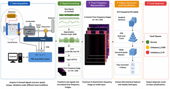
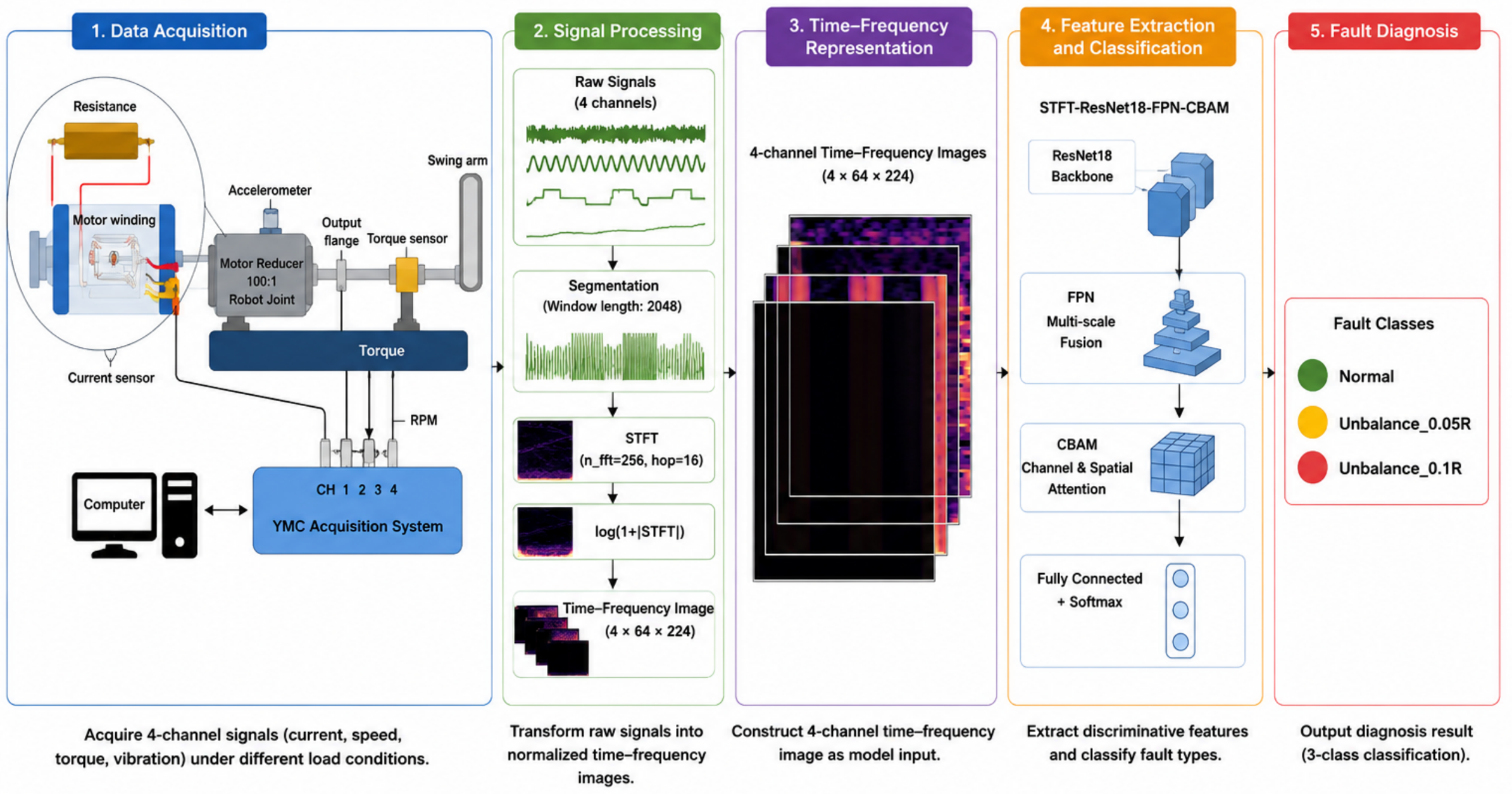
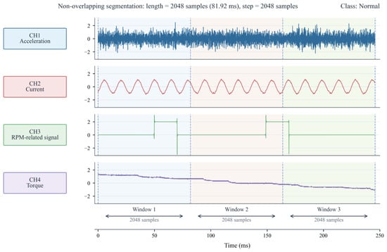
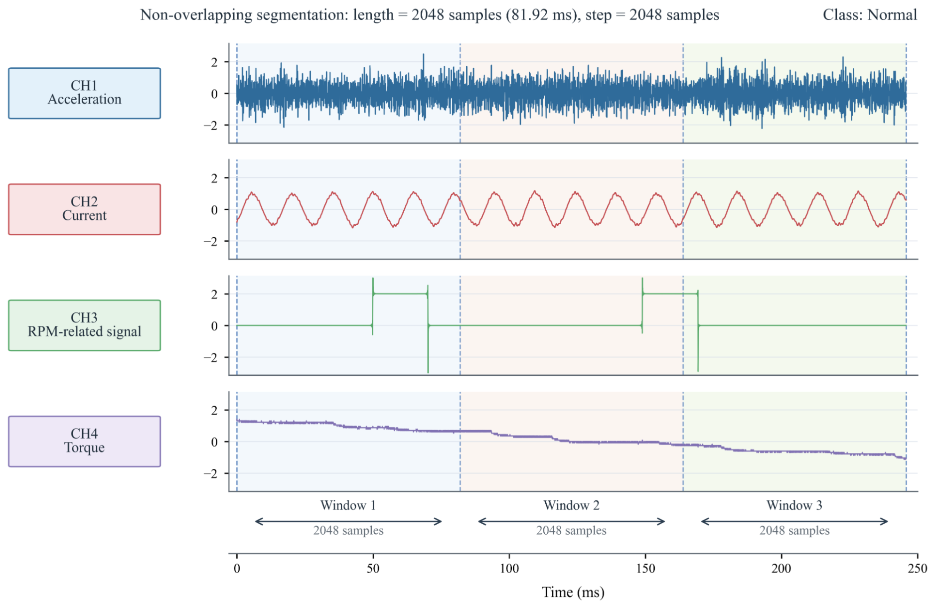
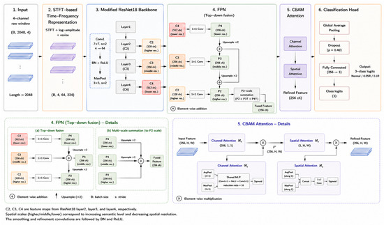
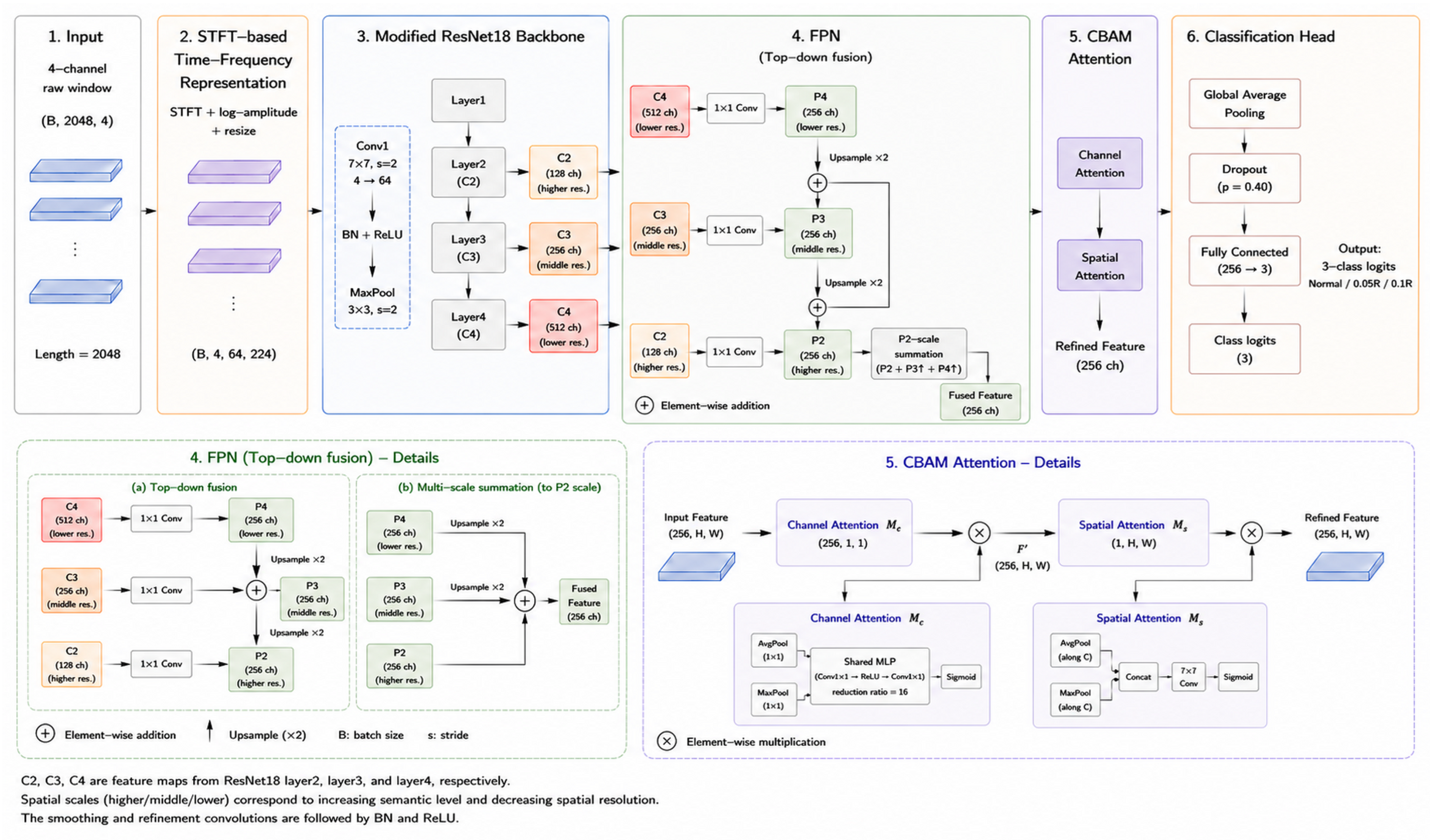
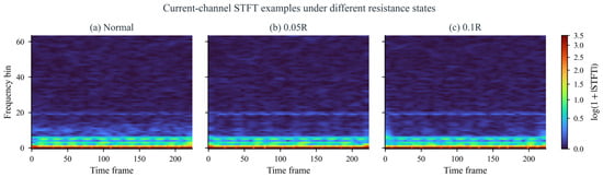
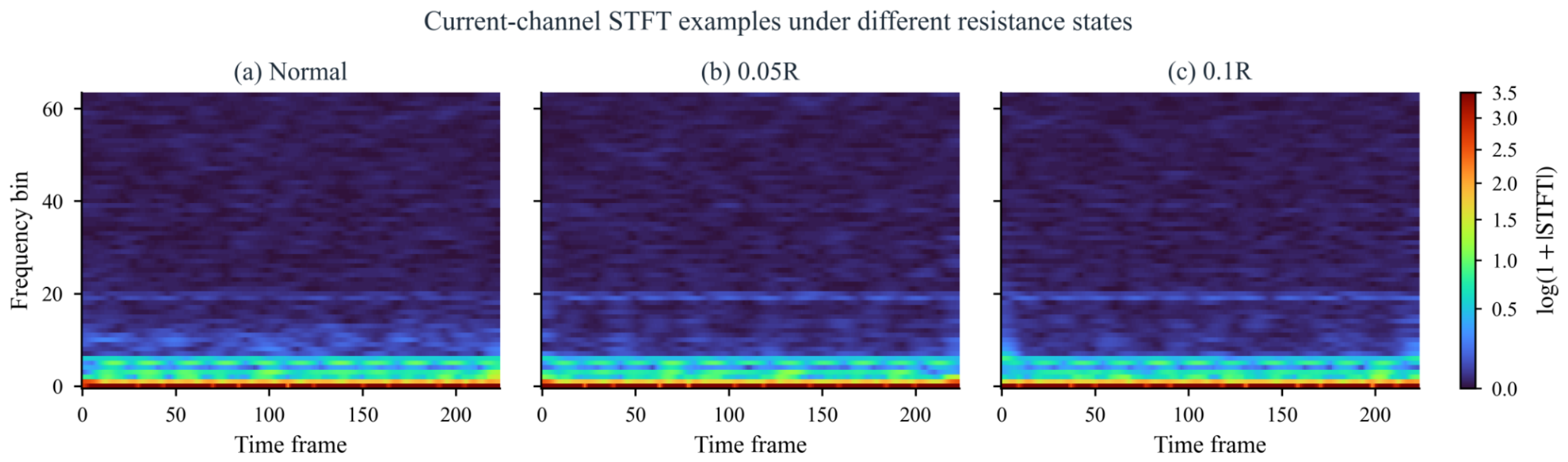
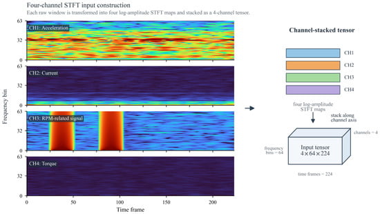
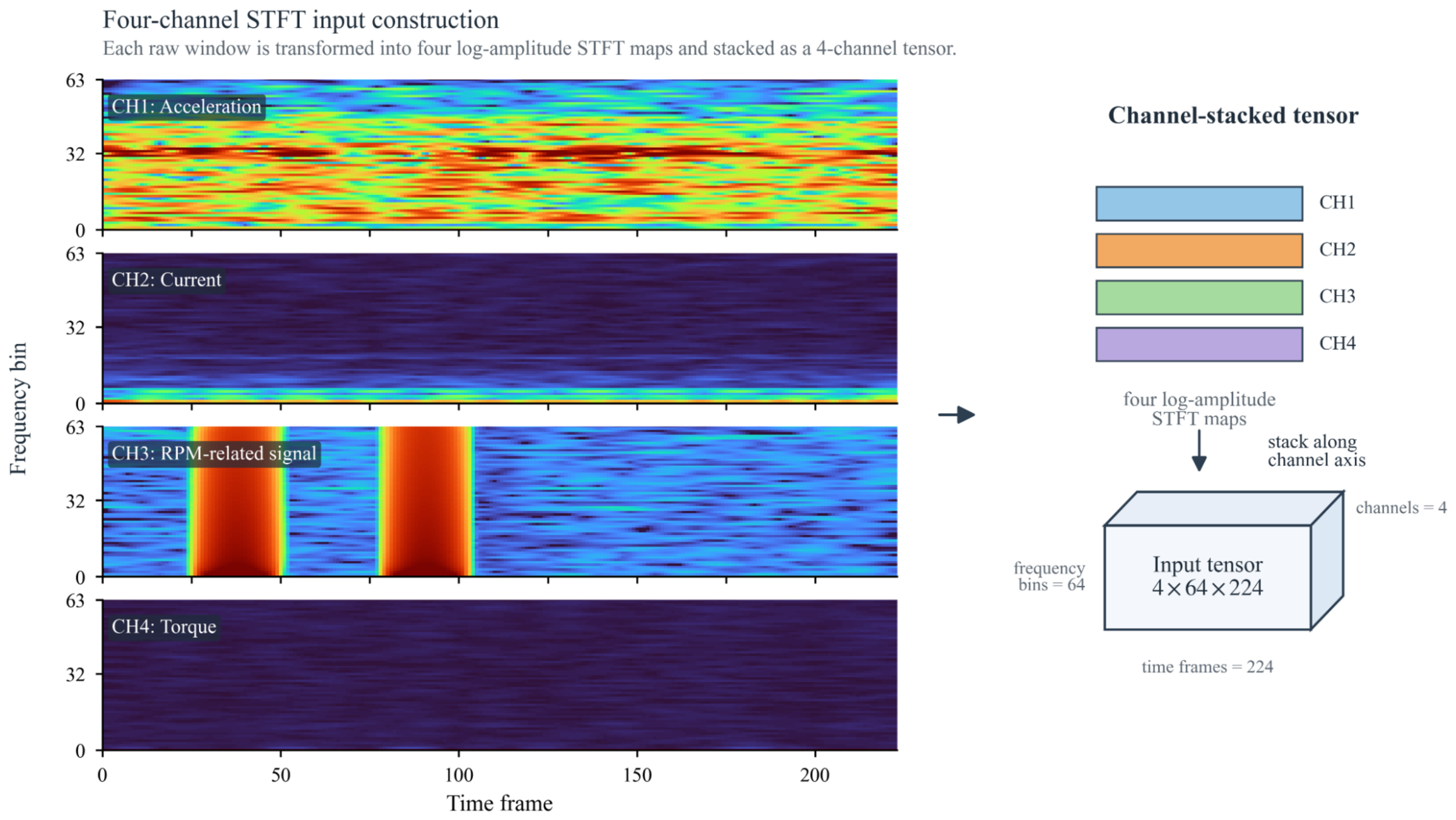
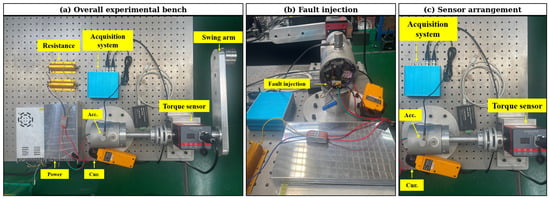
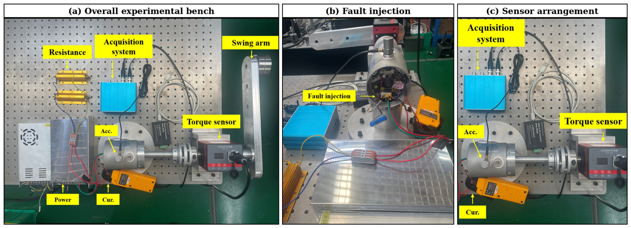
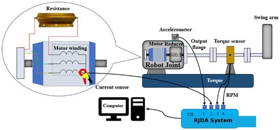
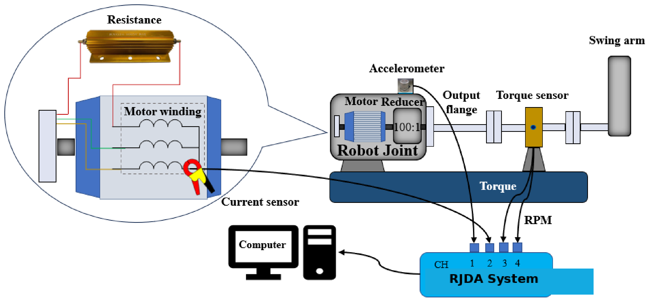
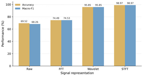
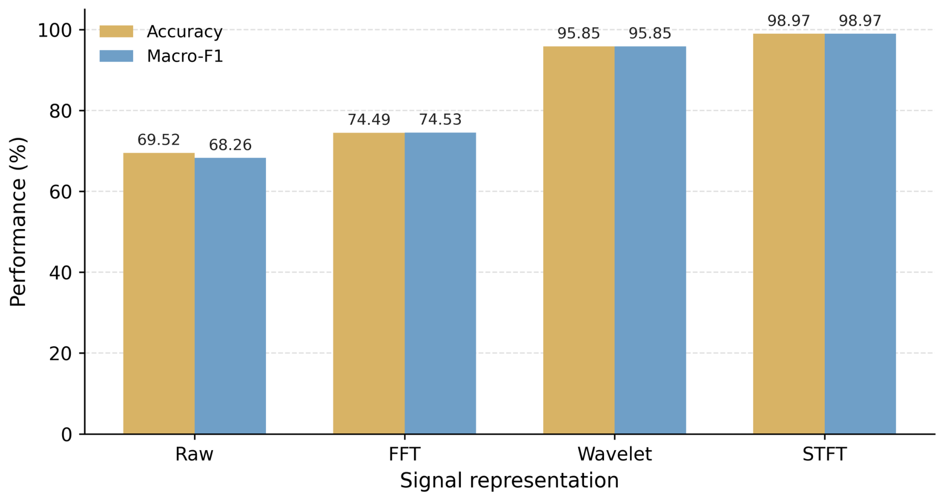
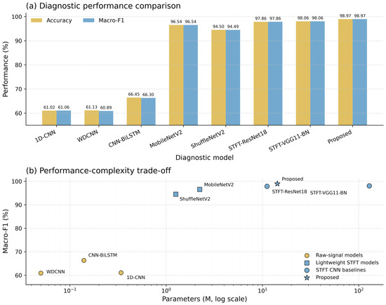
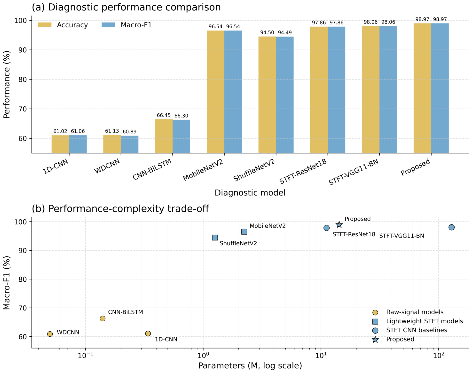
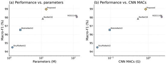
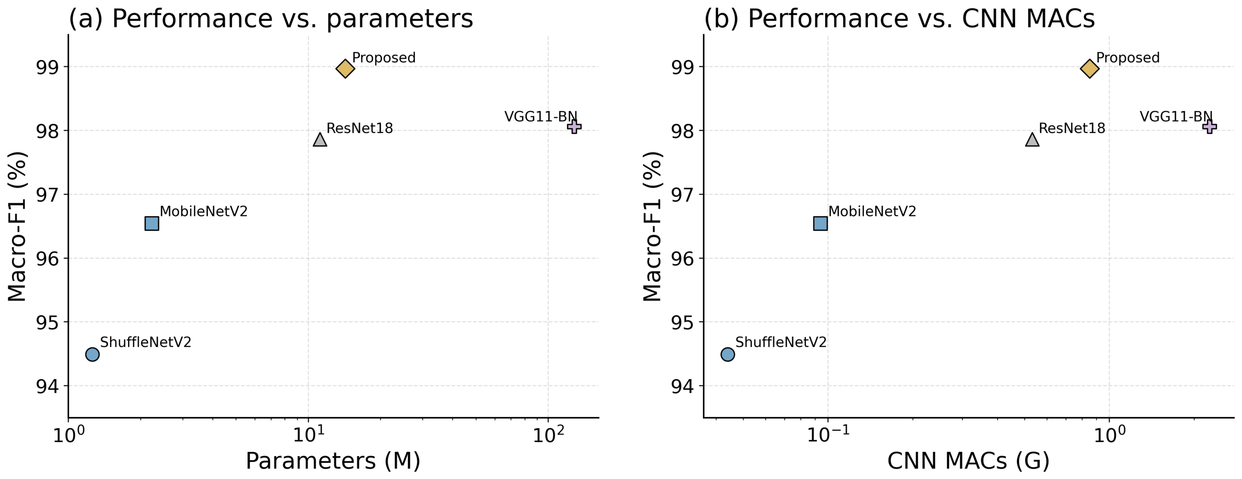
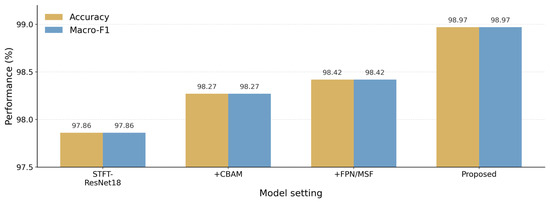
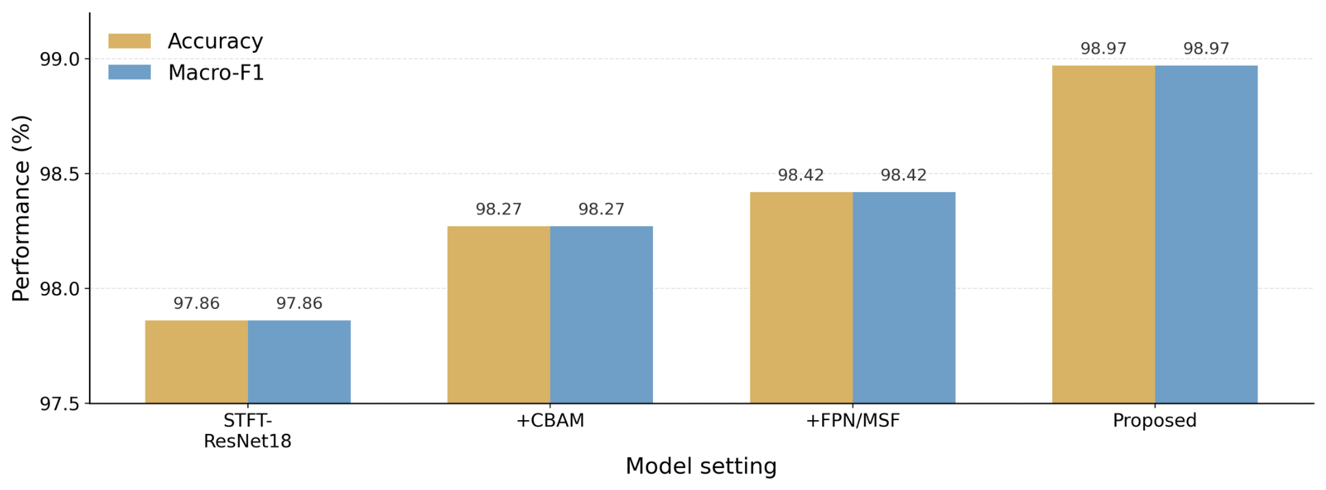
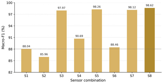
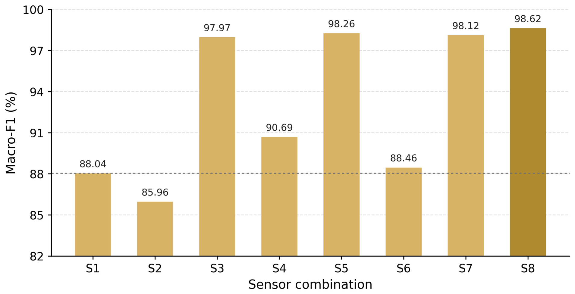
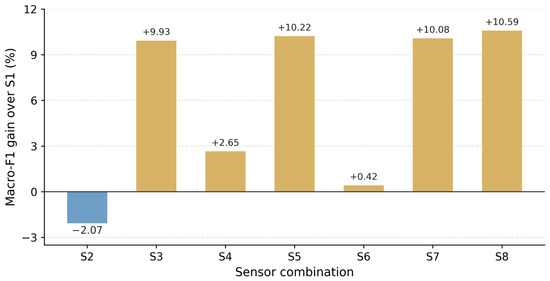
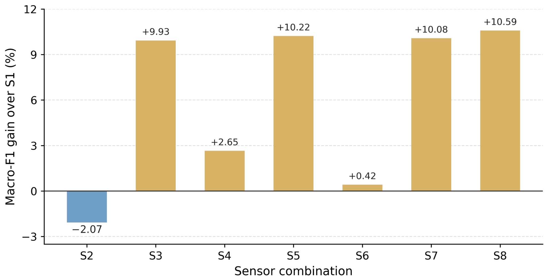
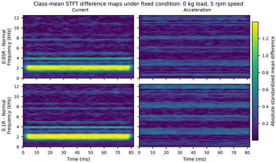
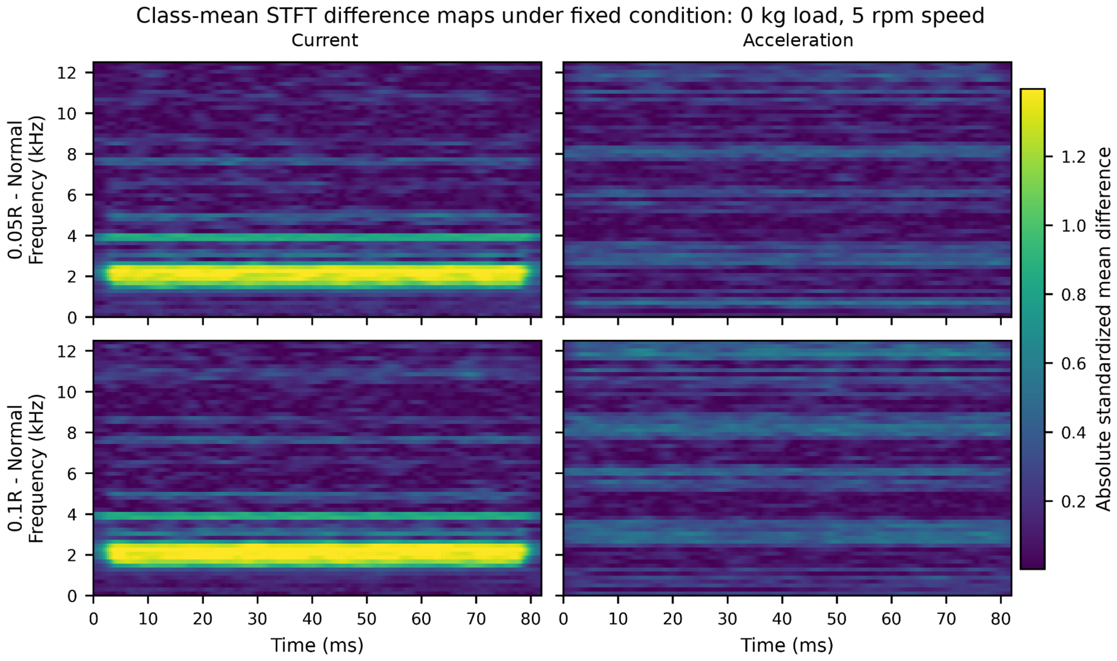
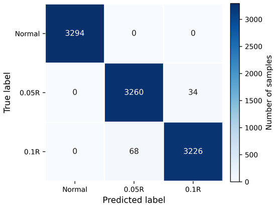
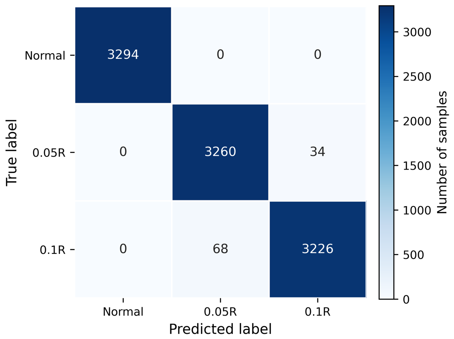
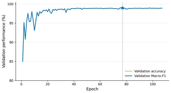
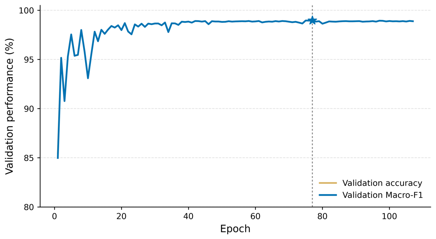
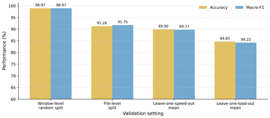
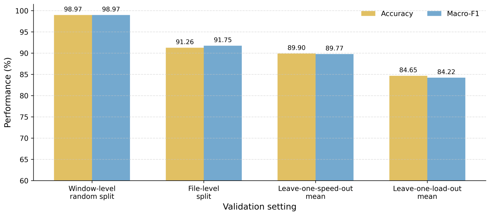
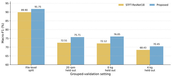
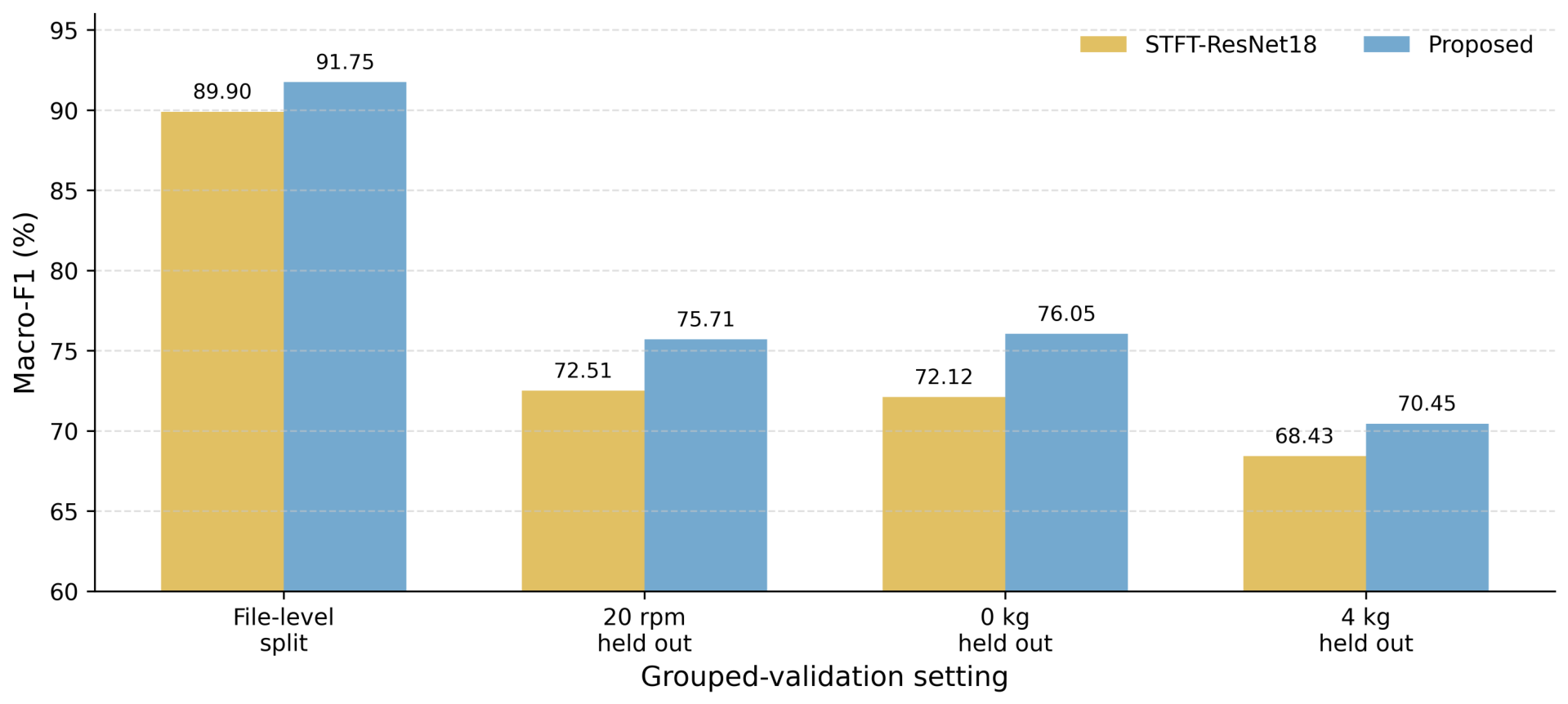
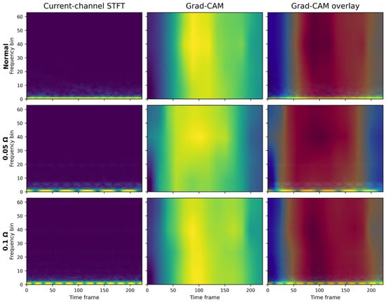
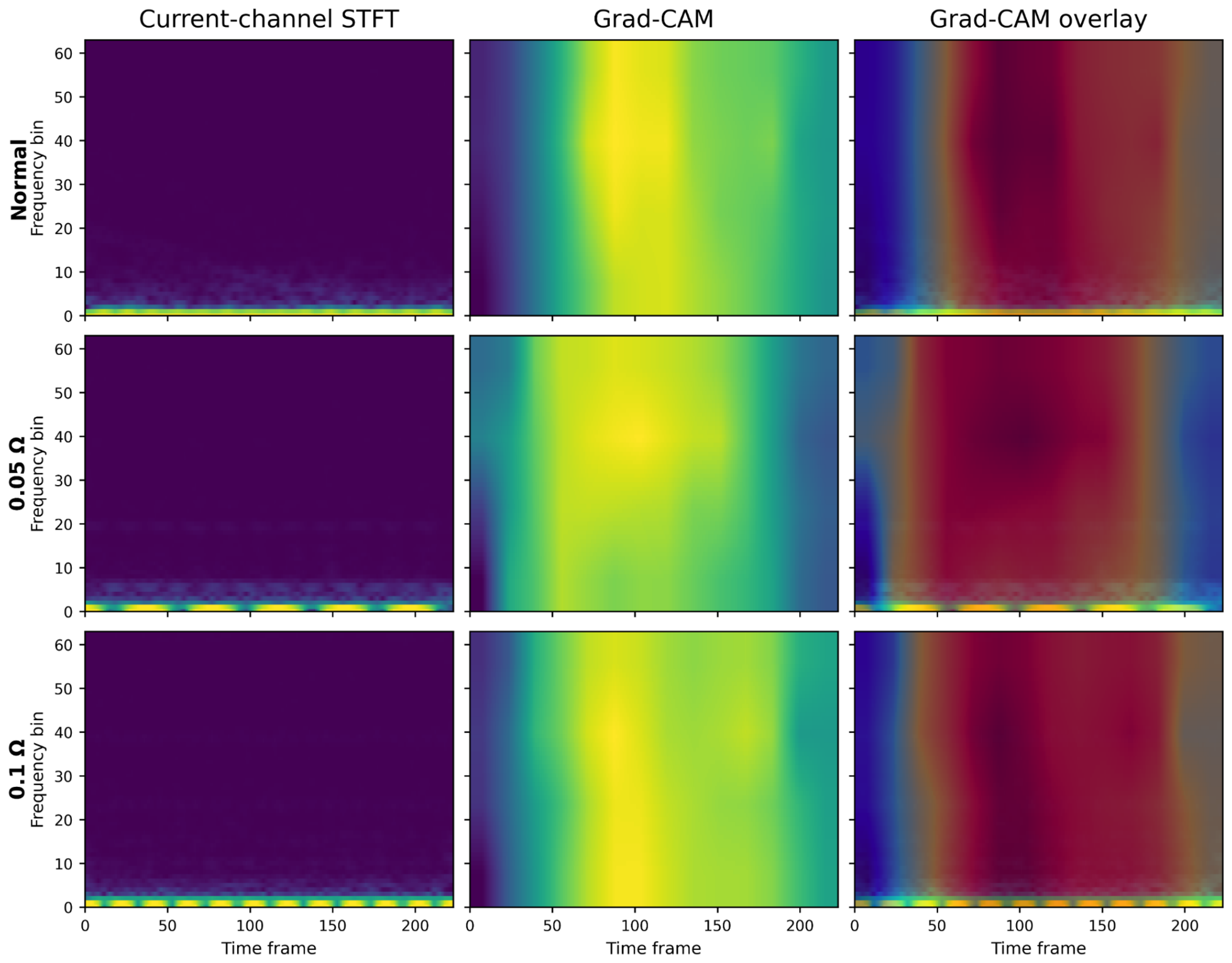

Disclaimer/Publisher’s Note: The statements, opinions and data contained in all publications are solely those of the individual author(s) and contributor(s) and not of MDPI and/or the editor(s). MDPI and/or the editor(s) disclaim responsibility for any injury to people or property resulting from any ideas, methods, instructions or products referred to in the content. |
© 2026 by the authors. Licensee MDPI, Basel, Switzerland. This article is an open access article distributed under the terms and conditions of the Creative Commons Attribution (CC BY) license.