Intelligent Condition Monitoring for Machining Processes Under Cross-Domain Scenarios via Semi-Supervised Feature Separation

Abstract

Tool wear state classification under varying working conditions remains challenging due to domain discrepancy and the scarcity of labeled target samples. To address this issue, this paper proposes a Semi-Supervised Domain-Adaptive Feature Separation framework (SS-DAFS) for intelligent condition monitoring in machining processes. Experiments are conducted on the PHM2010 milling dataset, where tool conditions are categorized into three health states, including initial wear, normal wear, and severe wear. The proposed framework separates shared domain-invariant features from private domain-specific features to enhance feature representation capability and reduce domain-specific interference. Meanwhile, Maximum Mean Discrepancy (MMD) is incorporated to further align feature distributions between source and target domains. Semi-supervised transfer tasks under one-shot and three-shot settings are constructed to evaluate the effectiveness of the proposed framework with extremely limited labeled target samples. Experimental results demonstrate that the proposed framework consistently outperforms several representative domain adaptation methods under both settings. The average accuracy of the proposed method under three-shot and one-shot achieves 95.68% and 94.34%, respectively. The results verify the effectiveness of the proposed framework for intelligent condition monitoring for machining processes under cross-domain machining scenarios.

1. Introduction

Tool condition monitoring (TCM) is widely recognized as a key enabling technology for intelligent manufacturing and predictive maintenance. Accurate monitoring of tool health conditions plays a crucial role in ensuring machining quality, dimensional accuracy, production efficiency, and operational safety while reducing manufacturing costs and unexpected machine downtime [1,2,3]. During machining operations, progressive tool wear inevitably degrades cutting performance, increases surface roughness, and may eventually result in catastrophic tool failure if timely intervention is not performed. Consequently, reliable tool condition monitoring has attracted considerable attention from both academia and industry and has become an essential component of modern smart manufacturing systems and Industry 4.0 [4,5].

With the rapid development of intelligent sensing technologies and artificial intelligence, large volumes of multisource monitoring data, including vibration, cutting force, acoustic emission, spindle current, and motor signals, can now be collected throughout the machining process. These data provide abundant information for evaluating tool health conditions and enable intelligent decision-making for predictive maintenance and production optimization [6,7]. Therefore, developing accurate and robust TCM methods has become an important research topic for improving manufacturing reliability, reducing maintenance costs, and promoting intelligent production.

In practical machining processes, tool wear is generally regarded as a progressive degradation phenomenon and can be categorized into multiple health states, such as initial wear, normal wear, and severe wear, according to the degree of flank wear and cutting performance degradation. Effective identification of these health states enables timely tool replacement and process optimization, thereby improving machining reliability and reducing maintenance costs. Consequently, intelligent tool health state classification has attracted increasing attention in recent years and has become a key research topic in machining process condition monitoring.

Traditional TCM approaches mainly rely on handcrafted feature extraction from sensor signals such as vibration, acoustic emission, cutting forces, and motor current, followed by classical machine learning algorithms such as support vector machines (SVMs), k-nearest neighbors (KNN), and random forests (RFs) [8,9,10]. Although these methods can achieve satisfactory performance under specific operating conditions, their generalization capability is often limited when machining parameters or working environments change. Moreover, manual feature engineering usually requires extensive domain expertise and considerable effort, which restricts the deployment of such approaches in practical industrial applications.

The rapid development of deep learning has revolutionized data-driven TCM. Convolutional neural networks (CNNs), recurrent neural networks (RNNs), and hybrid architectures can automatically learn hierarchical and discriminative feature representations from raw sensor data, eliminating the need for handcrafted features [11,12,13]. Deep learning-based models have been successfully applied to tool wear classification and remaining useful life prediction, showing superior performance compared with traditional methods [14,15]. For example, Zou et al. [16] proposed a feature-weighted convolutional neural network for tool wear identification under imbalanced samples. Xue et al. [17] proposed a hierarchical temporal transformer network for tool wear condition monitoring and verified its capability on the PHM2010 dataset. Martínez-Arellano et al. [18] used Gramian angular summation fields to image the time-series data and conducted tool wear classification using CNNs. Nevertheless, most existing deep learning approaches assume that training and testing data follow the same distribution. In real manufacturing environments, variations in cutting speed, feed rate, tool geometry, and workpiece material often lead to significant distribution shifts, known as domain discrepancies. These shifts severely degrade the performance of conventional deep models when applied to unseen tools or different operating conditions [19].

To mitigate the domain shift problem, domain adaptation (DA) techniques have been increasingly adopted in intelligent manufacturing [20,21,22]. DA methods aim to reduce the discrepancy between source and target domains by learning domain-invariant representations. Prominent approaches include adversarial learning-based methods [23], discrepancy minimization methods such as Maximum Mean Discrepancy (MMD) and correlation alignment [24], and feature disentanglement techniques [25]. These strategies have demonstrated promising results in cross-domain fault diagnosis and tool wear prediction, showing enhanced robustness under varying working conditions. For example, Huang et al. [26] proposed a cross-domain adaptation network based on a joint distribution adaptation method for tool wear prediction; Li et al. [27] proposed a novel tool wear state prediction method based on feature-based transfer learning, which used MMD to measure the similarity of features. Zhu et al. [28] proposed an unsupervised dual-regression domain adversarial adaption network for tool wear prediction based on adversarial training and Wasserstein distance. However, most existing studies focus on fully unsupervised domain adaptation, where no labeled target samples are assumed. In industrial practice, obtaining a small number of labeled target samples is often feasible and cost-effective, while labeling large-scale datasets remains labor-intensive. Consequently, semi-supervised domain adaptation (SSDA) has emerged as a practical and promising solution, leveraging a few labeled target samples in combination with abundant source domain data to improve cross-domain learning [29,30,31].

Recent advances in SSDA have demonstrated that incorporating a small number of labeled target-domain samples can significantly improve cross-domain classification performance. Representative SSDA methods, such as Minimax Entropy(MME) [29], Cross-Domain Adaptive Clustering(CDAC) [32], and adversarial learning-based approaches, mainly exploit target-domain supervision through entropy minimization, consistency regularization, decision boundary refinement, or adversarial feature alignment. Although these methods have achieved encouraging results in image recognition tasks, they are not specifically designed for tool condition monitoring, where complex operating conditions often lead to substantial domain shifts and highly coupled feature distributions. Moreover, most existing methods primarily focus on aligning global feature distributions while paying limited attention to disentangling domain-invariant and domain-specific representations. As a result, domain-specific interference may still be embedded in the learned shared features, thereby reducing the discriminative capability and transferability of the model. Furthermore, under extremely limited target-domain supervision, the scarcity of labeled samples further aggravates inaccurate feature alignment and deteriorates the generalization performance of existing SSDA methods.

To address these limitations, this paper proposes a novel SS-DAFS framework for intelligent tool condition monitoring. Unlike existing SSDA methods, the proposed framework explicitly separates shared domain-invariant features from domain-specific features through dedicated feature extractors and introduces a feature separation strategy to reduce redundant domain-specific interference. Meanwhile, MMD is employed to further align the shared feature distributions across domains, enabling the model to learn more discriminative and transferable representations. By effectively integrating feature separation and distribution alignment, the proposed method achieves robust cross-domain tool condition monitoring under limited labeled target samples and demonstrates superior performance compared with existing state-of-the-art SSDA approaches. Experiments are conducted on the PHM2010 milling dataset [33]. Tool health states are categorized into three classes: initial wear, normal wear, and severe wear. 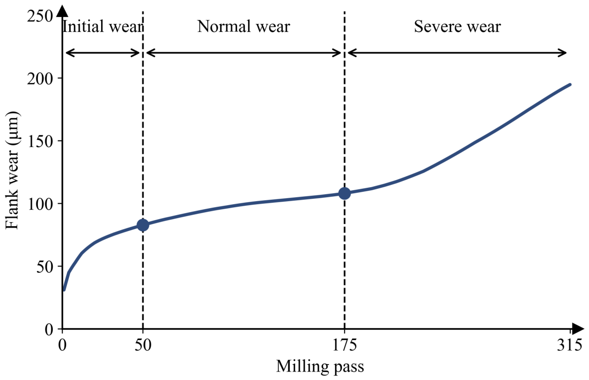Figure 1 illustrates the wear process of the cutting tool during its life cycle.

The main contributions of this paper are summarized as follows:

• A semi-supervised domain-adaptive feature separation framework is proposed for cross-domain tool wear state classification. The proposed framework adopts a dual encoder architecture that separates domain-invariant shared representations from domain-specific private representations.
• A feature separation constraint is introduced to reduce the correlation between shared and private representations, encouraging the shared features to retain only wear-state discriminative information while suppressing operating-condition-specific interference.
• Extensive experiments on the PHM2010 dataset under one-shot and three-shot settings demonstrate that the proposed method achieves superior classification performance and robust generalization capability compared with existing domain adaptation methods.

The remainder of this paper is organized as follows: Section 2 presents the preliminaries of this study. Section 3 illustrates the proposed method in detail. The experimental results are presented in Section 4. Finally, Section 5 summarizes the contribution of this paper and presents future work.

2. Preliminaries

2.1. Problem Definition of Semi-Supervised Domain Adaptation

In semi-supervised domain adaptation (SSDA), the source domain contains abundant labeled samples, while the target domain contains only a few labeled samples together with a large number of unlabeled samples [29]. Let the labeled source domain be defined as:

$${\mathcal{D}}_s={\left\{\left(x_i^s,y_i^s\right)\right\}}_{i=1}^{N_s},$$

(1)

where $x_i^s\in {\mathcal{X}}_s$ represents the source sample, $y_i^s\in {\mathcal{Y}}_s$ denotes the corresponding class label, and $N_s$ is the number of source samples. Similarly, the target domain consists of a small labeled subset and a large unlabeled subset, defined as [32]:

$${\mathcal{D}}_t^l={\left\{\left(x_i^t,y_i^t\right)\right\}}_{i=1}^{N_t^l},$$

(2)

and

$${\mathcal{D}}_t^u={\left\{x_i^t\right\}}_{i=1}^{N_t^u},$$

(3)

where $N_t^l\ll N_t^u$. In this study, the target domain labels correspond to three tool health states, including initial wear, normal wear, and severe wear.

Although the source domain and target domain share the same label space,

$${\mathcal{Y}}_s={\mathcal{Y}}_t,$$

(4)

their marginal probability distributions are different due to varying machining conditions:

$$P\left(X_s\right)\ne P\left(X_t\right).$$

(5)

This distribution discrepancy significantly degrades the performance of conventional deep learning models trained solely on source-domain data. Therefore, the objective of SSDA is to learn transferable and discriminative representations by utilizing labeled source samples, limited labeled target samples, and unlabeled target samples simultaneously.

Compared with fully supervised learning, SSDA is more suitable for practical industrial scenarios because obtaining a small number of labeled target samples is feasible, while large-scale data annotation remains labor-intensive and expensive.

2.2. Maximum Mean Discrepancy

Although feature separation learning can partially reduce domain discrepancy, the distributions of shared representations extracted from source and target domains may still remain inconsistent. Therefore, Maximum Mean Discrepancy (MMD) is introduced to further align feature distributions across domains [34].

MMD is a statistical metric used to measure the distribution discrepancy between two domains in reproducing kernel Hilbert space (RKHS). The MMD loss is formulated as [34]:

$${\mathcal{L}}_{mmd}={∥{\displaystyle \frac{1}{n_s}}{\displaystyle \sum _{i=1}^{n_s}}\varphi \left(z_i^s\right)-{\displaystyle \frac{1}{n_t}}{\displaystyle \sum _{j=1}^{n_t}}\varphi \left(z_j^t\right)∥}_{\mathcal{H}}^2,$$

(6)

where $\varphi (·)$ denotes the nonlinear mapping function in RKHS, and $n_s$ and $n_t$ represent the numbers of source and target samples, respectively.

Minimizing the MMD loss encourages the shared feature distributions of different domains to become similar, thereby improving domain alignment capability and enhancing cross-domain classification performance. In this study, a multi-kernel Gaussian kernel is adopted to calculate the MMD loss for improving distribution alignment capability.

2.3. Motivation of the Proposed Method

In practical tool wear monitoring scenarios, varying machining conditions often introduce significant domain discrepancies between source and target datasets. Existing domain adaptation methods mainly focus on feature alignment while neglecting the interference caused by entangled domain-specific information. Moreover, under low-shot target scenarios, such as one-shot and three-shot settings, insufficient target supervision further increases the difficulty of learning transferable representations.

Motivated by feature separation learning and domain distribution alignment, the proposed SS-DAFS framework combines shared-private feature disentanglement with MMD-based domain alignment for semi-supervised cross-domain tool wear classification. The proposed framework aims to simultaneously preserve discriminative tool wear information and reduce domain discrepancy, thereby improving classification accuracy and generalization capability under limited labeled target samples.

3. Proposed Method

3.1. Overview of the Proposed Framework

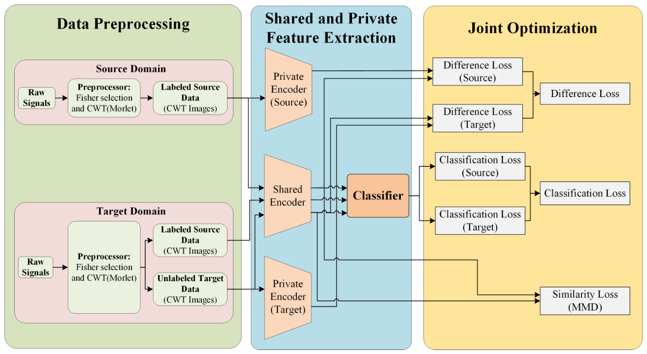
The overall architecture of the proposed Semi-Supervised Domain-Adaptive Feature Separation (SS-DAFS) framework is illustrated in Figure 2. The proposed framework is designed for cross-domain tool wear state classification under limited labeled target samples. Specifically, the framework consists of a shared feature encoder, two domain-specific private encoders, a task classifier, and multiple optimization constraints. The shared encoder and the two private encoders together form a dual encoder architecture that explicitly decomposes the input representation into domain-invariant and domain-specific components. This decomposition-then-alignment design is the key methodological feature that distinguishes the proposed framework from prior SSDA methods relying on a single shared encoder with global feature alignment.

Given source domain samples and target domain samples, the shared encoder is employed to extract domain-invariant representations associated with tool wear states, while the private encoders are utilized to preserve domain-specific information caused by varying machining conditions. The extracted shared representations are subsequently fed into the classifier for health state prediction. To further improve cross-domain representation learning, Maximum Mean Discrepancy (MMD) loss is introduced to align the shared feature distributions between source and target domains. Meanwhile, a difference loss is employed to reduce the correlation between shared representations and private representations, thereby improving feature disentanglement capability.

Through joint optimization of source classification loss, target classification loss, MMD loss, and difference loss, the proposed framework aims to learn robust and transferable representations for semi-supervised cross-domain tool wear state classification.

3.2. Data Preprocessing

The PHM2010 milling dataset was adopted in this study to evaluate the effectiveness of the proposed framework. The original monitoring dataset contains multiple sensor signals collected during the milling process, including vibration signals and cutting force signals. Since raw time-series signals usually exhibit complex non-stationary characteristics, an effective preprocessing strategy is required to improve feature representation capability.

First, the Fisher Score is employed to evaluate the discriminative capability of different sensor channels. The Fisher Score of the kth channel is defined as

$$F_k={\displaystyle \frac{{\sum }_{c=1}^C{n}_c{({\mu }_c-\mu )}^2}{{\sum }_{c=1}^C{\sum }_{i=1}^{n_c}{(x_i^c-{\mu }_c)}^2}},$$

(7)

where C denotes the number of classes, $n_c$ represents the number of samples in the cth class, ${\mu }_c$ denotes the mean value of the cth class, and $\mu$ represents the global mean value.

After channel selection, a Continuous Wavelet Transform (CWT) is applied to convert one-dimensional sensor signals into time–frequency representations. The CWT can be formulated as

$$W(a,b)={\displaystyle \frac{1}{\sqrt{a}}}{\int }_{-\infty }^{+\infty }x\left(t\right){\psi }^{*}\left({\displaystyle \frac{t-b}{a}}\right)dt,$$

(8)

where a and b denote the scale factor and translation factor, respectively, and $\psi (·)$ represents the mother wavelet function. In this study, the Morlet wavelet was adopted as the mother wavelet. The Morlet wavelet is a complex sinusoid modulated by a Gaussian envelope, providing the best attainable joint time–frequency concentration among admissible wavelets [35]. In addition, its oscillatory and amplitude-modulated waveform closely resembles the quasi-periodic impulsive components induced by tool–workpiece interaction and progressive wear in the cutting force signals, so that the resulting scalograms preserve wear-related transient information while remaining smooth and well localized. This property makes the Morlet wavelet a common choice for time–frequency analysis in machinery condition monitoring [36,37].

The generated time–frequency maps from the selected channels are stacked as RGB images and resized to $224\times 224$ pixels. Subsequently, all images are normalized using the standard ImageNet z-score normalization. Specifically, the pixel values of each channel are first scaled to the range [0, 1], and then standardized using the channel-wise mean $\mu =[0.485,0.456,0.406]$ and standard deviation $\sigma =[0.229,0.224,0.225]$ computed from the ImageNet dataset. This normalization strategy is consistent with the commonly adopted preprocessing pipeline for ImageNet-pretrained backbone networks. The normalized images are used as the input of the proposed framework.

According to the tool wear progression characteristics in the PHM2010 dataset, the milling process was divided into three health states based on the number of milling passes. The detailed definitions of tool wear states are summarized in

Table 1. Definition of tool wear health states in the PHM2010 dataset.

Health State	Milling Pass Range
Initial wear	1–50
Normal wear	51–175
Severe wear	176–315

.

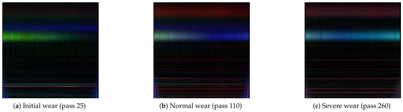
Figure 3 presents the time–frequency maps of different wear states. To evaluate the semi-supervised cross-domain capability of the proposed framework, 1-shot and 3-shot transfer tasks were constructed using the C1, C4, and C6 cutter datasets.

3.3. Shared and Private Feature Extraction

In practical machining environments, monitoring signals generally contain both domain-invariant degradation information and domain-specific characteristics related to varying machining conditions. To effectively disentangle these two types of information, the proposed framework adopts a dual encoder architecture, consisting of one shared encoder and two domain-specific private encoders.

Given an input sample x, the shared representation is defined as

$$z_s=E_s\left(x\right),$$

(9)

where $E_s(·)$ denotes the shared encoder. The shared representation aims to capture transferable discriminative information associated with tool wear states.

Meanwhile, the source-domain private representation and target-domain private representation are extracted as

$$z_p^s=E_p^s\left(x_s\right),$$

(10)

and

$$z_p^t=E_p^t\left(x_t\right),$$

(11)

where $E_p^s(·)$ and $E_p^t(·)$ denote the source private encoder and target private encoder, respectively. These private representations mainly preserve domain-specific characteristics caused by varying operating conditions.

In this study, ResNet34 was employed as the backbone network of the shared encoder due to its superior feature extraction capability. Meanwhile, lightweight ResNet18 networks were adopted as private encoders to reduce computational complexity while preserving domain-specific information.

3.4. Difference Loss

To further enhance feature disentanglement capability, a difference loss is introduced to reduce the correlation between shared representations and private representations. Specifically, the shared features and private features are first normalized along the feature dimension:

$${\widehat{H}}_s={\displaystyle \frac{H_s}{\parallel H_s{\parallel }_2}},$$

(12)

and

$${\widehat{H}}_p={\displaystyle \frac{H_p}{\parallel H_p{\parallel }_2}},$$

(13)

where $H_s$ and $H_p$ denote the shared feature matrix and private feature matrix, respectively.

Subsequently, the correlation matrix between normalized shared features and normalized private features is calculated as

$$C={\widehat{H}}_s^T{\widehat{H}}_p.$$

(14)

The difference loss is defined as

$${\mathcal{L}}_{diff}={\displaystyle \frac{1}{N}}{∥C∥}_F^2,$$

(15)

where N denotes the batch size and ${\parallel ·\parallel }_F$ represents the Frobenius norm.

Minimizing the difference loss encourages the shared feature space and private feature space to become orthogonal, thereby reducing feature redundancy and improving feature disentanglement capability.

3.5. Semi-Supervised Classification Loss

The shared representations extracted from both source and target domains are fed into the classifier for tool wear state prediction. The source-domain classification loss is defined as

$${\mathcal{L}}_{src}=-{\displaystyle \frac{1}{N_s}}{\displaystyle \sum _{i=1}^{N_s}}{y}_i^{s}log\left({\widehat{y}}_i^s\right),$$

(16)

where $y_i^s$ and ${\widehat{y}}_i^s$ denote the ground-truth label and predicted probability of the source sample, respectively.

Similarly, the labeled target samples are also utilized for supervised learning. The target-domain classification loss is formulated as

$${\mathcal{L}}_{tgt}=-{\displaystyle \frac{1}{N_t}}{\displaystyle \sum _{i=1}^{N_t}}{y}_i^{t}log\left({\widehat{y}}_i^t\right),$$

(17)

where $y_i^t$ and ${\widehat{y}}_i^t$ denote the ground-truth label and predicted probability of the target sample, respectively.

The total classification loss is then defined as

$${\mathcal{L}}_{cls}={\mathcal{L}}_{src}+{\mathcal{L}}_{tgt}.$$

(18)

By jointly utilizing labeled source samples and limited labeled target samples, the proposed framework can effectively improve classification performance under low-shot target scenarios.

3.6. Overall Objective Function

The total optimization objective of the proposed framework consists of classification loss, MMD loss, and difference loss:

$${\mathcal{L}}_{total}={\mathcal{L}}_{cls}+{\alpha }_{diff}{\mathcal{L}}_{diff}+{\alpha }_{sim}{\mathcal{L}}_{mmd},$$

(19)

where ${\alpha }_{diff}$ and ${\alpha }_{sim}$ denote the weighting coefficients of the difference loss and MMD loss, respectively.

Through joint optimization of multiple objectives, the proposed SS-DAFS framework can simultaneously learn discriminative domain-invariant representations and preserve domain-specific characteristics, thereby improving semi-supervised cross-domain tool wear state classification performance under varying working conditions. The overall training procedure of the proposed SS-DAFS framework is presented in Algorithm 1.

Algorithm 1 Training procedure of SS-DAFS.

Require: Source data ${\mathcal{D}}_s$, labeled target data ${\mathcal{D}}_t^l$, unlabeled target data ${\mathcal{D}}_t^u$   1: for each training iteration do   2:     Sample mini-batches from ${\mathcal{D}}_s$, ${\mathcal{D}}_t^l$, and ${\mathcal{D}}_t^u$   3:     Extract shared features: $$z_s^s=E_s\left(x_s\right),z_s^t=E_s\left(x_t^u\right)$$   4:     Extract private features: $$z_p^s=E_p^s\left(x_s\right),z_p^t=E_p^t\left(x_t^u\right)$$   5:     Compute source classification loss: $${\mathcal{L}}_{src}=CE(C\left(z_s^s\right),y_s)$$   6:     Compute labeled target classification loss: $${\mathcal{L}}_{tgt}=CE(C\left(E_s\left(x_t^l\right)\right),y_t^l)$$   7:     Compute difference loss: $${\mathcal{L}}_{diff}=Diff(z_s^s,z_p^s)+Diff(z_s^t,z_p^t)$$   8:     Compute MMD loss: $${\mathcal{L}}_{mmd}=MMD(z_s^s,z_s^t)$$   9:     Compute total loss: $$\mathcal{L}={\mathcal{L}}_{src}+{\mathcal{L}}_{tgt}+{\alpha }_{diff}{\mathcal{L}}_{diff}+{\alpha }_{sim}{\mathcal{L}}_{mmd}$$  10:     Update all network parameters  11: end for

4. Experimental Validation

4.1. Dataset Description

To evaluate the effectiveness of the proposed SS-DAFS framework, experiments were conducted on the PHM2010 milling tool wear dataset released by the Prognostics and Health Management Society [33]. The PHM2010 dataset is widely adopted in intelligent manufacturing research for tool condition monitoring and tool wear prediction under varying machining conditions.

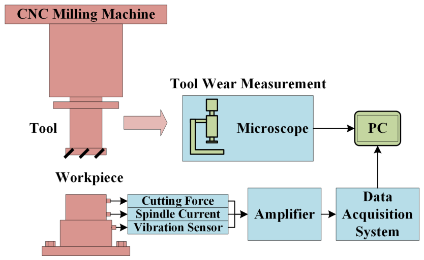
The dataset contains multiple run-to-failure milling experiments collected from a high-speed CNC milling machine Röder Tech RFM760 (Röders GmbH, Soltau, Germany). HRC52 stainless steel was used as the workpiece material. During the milling process, several sensor signals were synchronously recorded, including vibration signals, spindle current, and cutting force signals. The cutting tools were three-flute tungsten carbide ball-nose end mills, corresponding to cutters C1, C4, and C6, and the milling was performed under dry, down-milling conditions. During the tests, tool wear was quantified by the flank wear (VB), namely, the width of the wear land on the flank face. After each milling pass, the flank wear of each of the three flutes was measured off-line using a microscope, and the average value of the three flutes was adopted as the final wear indicator, based on which, the initial, normal, and severe wear states were defined. Figure 4 illustrates the experimental setup of the PHM2010 dataset.

Table 2. Cutting setting of the experimental dataset.

Cutting Parameters	Value
Feed rate (mm/min)	1555
Spindle speed (r/min)	10,400
Feed volume (mm)	0.001
Axial depth of cut (mm)	0.2
Radial cutting width (mm)	0.125
Sampling frequency (kHz)	50

presents the details of cutting parameters. In this study, Fisher Score analysis was first conducted to evaluate the discriminative capability of different sensor channels. Experimental results indicated that the three-axis cutting force signals exhibited superior discriminative performance compared with other monitoring signals. Therefore, the three-axis cutting force data were selected as the monitoring signals for subsequent experiments.

Three cutters, namely, C1, C4, and C6, were adopted to construct cross-domain transfer tasks. Different cutters correspond to different operating conditions and exhibit obvious distribution discrepancies caused by variations in machining environments and degradation processes. Therefore, these datasets are suitable for evaluating the cross-domain generalization capability of semi-supervised domain adaptation methods.

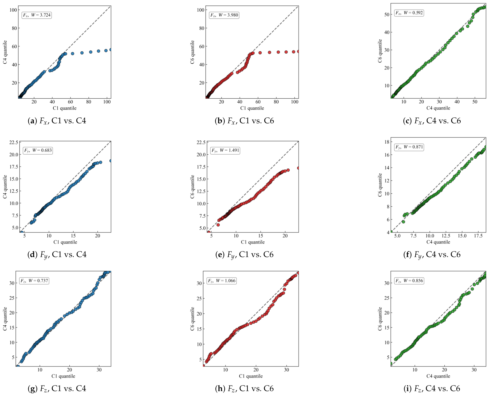
To characterize this discrepancy quantitatively, the per-cut RMS distributions of the three-axis cutting force were compared across the three cutters through the quantile–quantile plots in Figure 5. Since all cutters shared identical cutting parameters as listed in Table 2, the observed shift originates not from the machining settings but from cutter-specific factors such as manufacturing tolerance and the divergent wear evolution of each tool. Systematic departures from the $y=x$ reference are observed for every force component and every cutter pair, and the annotated one-Wasserstein distance W provides a numerical measure of the gap. The discrepancy is most pronounced on the $F_x$ component between C1 and the other two cutters ($W=3.724$ and $3.980$), while C4 and C6 remain comparatively close ($W=0.592$).

Following the preprocessing strategy described in Section 3, a CWT was utilized to convert one-dimensional cutting force signals into two-dimensional time–frequency representations. The generated time–frequency maps from the selected three-axis cutting force channels were stacked into RGB images and resized to $224\times 224$ pixels before being fed into the network.

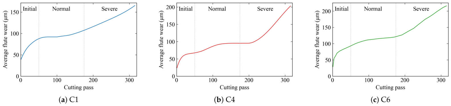
Based on the averaged wear values, the wear evolution curves of cutters C1, C4, and C6 were plotted to illustrate the degradation process under different operating conditions, as shown in Figure 6. The milling process was divided into three health states based on the number of milling passes. The detailed definitions of tool wear states are summarized in Table 1.

From a machining perspective, flank wear does not progress uniformly but follows three characteristic stages. In the initial break-in stage, the sharp cutting edge wears rapidly over a short period; in the normal wear stage, the wear land grows slowly and steadily, which constitutes the major portion of the tool life; in the severe wear stage, the wear accelerates and may quickly lead to tool failure. These three stages provide the physical basis for dividing the milling process into the initial, normal, and severe health states.

This wear progression was directly reflected in the cutting force signals. As the flank wear land widened, the increased flank–workpiece contact and friction raised the amplitude of the three-axis cutting force, while the intensified rubbing and micro-impacts in the severe stage introduced stronger high-frequency components. Since both the magnitude and the time–frequency distribution of the force evolved monotonically with the wear state, the three-axis cutting force was identified as the most discriminative signal by the Fisher Score analysis, and its CWT time–frequency representation was adopted as the network input.

To evaluate the performance of the proposed framework under limited labeled target samples, semi-supervised transfer tasks were designed under one-shot and three-shot settings. Specifically, the source domain contained sufficient labeled samples, while only one or three labeled samples per class were provided in the target domain. The remaining target samples were treated as unlabeled data during training. Such experimental settings are consistent with practical industrial scenarios, where obtaining a large number of labeled target samples is usually difficult and labor-intensive.

4.2. Comparison Methods and Experimental Settings

To comprehensively evaluate the effectiveness of the proposed SS-DAFS framework, several representative domain adaptation methods were selected as comparison models, including Source Only, MMD [34], Domain-Adversarial Neural Network (DANN) [38], Adversarial Discriminative Domain Adaptation (ADDA) [39], Minimax Entropy (MME) [29], and Cross-Domain Adaptive Clustering (CDAC) [32].

• Source Only: A baseline model trained only using labeled source-domain samples without any domain adaptation strategy.
• MMD [34]: A discrepancy-based domain adaptation method that minimizes the distribution discrepancy between source and target domains using Maximum Mean Discrepancy.
• DANN [38]: An adversarial domain adaptation method that employs a gradient reversal layer to learn domain-invariant representations.
• ADDA [39]: An adversarial adaptation framework that aligns target-domain features with source-domain features through adversarial learning.
• MME [29]: A semi-supervised domain adaptation method based on minimax entropy optimization to improve target-domain decision boundaries.
• CDAC [32]: A semi-supervised domain adaptation approach that combines adaptive clustering and consistency regularization for cross-domain classification.

For a fair comparison, all methods were implemented under the same experimental settings and utilized identical preprocessing strategies and backbone networks whenever possible.

All experiments were implemented in Python 3.10 using the PyTorch 1.12 deep learning framework. The experiments were conducted on a laptop equipped with an AMD Ryzen 9 5900 CPU, 16 GB of RAM, and an NVIDIA RTX 3060 GPU.

In this study, stochastic gradient descent (SGD) with Nesterov momentum was adopted for network training, where the momentum coefficient and the weight decay followed common practice and were set to 0.9 and $5\times {10}^{-4}$, respectively. The remaining key hyperparameters, including the initial learning rate, the batch size, the number of warm-up iterations, and the weighting coefficients ${\alpha }_{diff}$ and ${\alpha }_{sim}$ of the difference loss and the MMD loss, were determined automatically using the Ray Tune framework, with the classification accuracy on the labeled target validation set as the optimization objective and the test data excluded from the search to avoid information leakage. The best configuration was obtained at an initial learning rate of 0.01 decayed by an inverse schedule, a batch size of 32, 1000 warm-up iterations, and ${\alpha }_{diff}={\alpha }_{sim}=0.1$. Each model was then trained for 3000 iterations under that configuration, and the detailed settings are summarized in

Table 3. Implementation details and hyperparameter settings. Hyperparameters marked with a search space were optimized automatically via Ray Tune.

Item	Search Space	Selected
Shared encoder	—	ResNet-34 (ImageNet-pretrained)
Private encoders	—	ResNet-18
Input size	—	$224\times 224\times 3$
Input normalization	—	ImageNet z-score
Optimizer	—	SGD (Nesterov), momentum $=0.9$
Weight decay	—	$5\times {10}^{-4}$
Initial learning rate	$\{0.001,0.005,0.01,0.05\}$	$0.01$
Learning-rate schedule	—	${\eta }_t={\eta }_0{(1+0.0001t)}^{-0.75}$
Batch size	$\{16,24,32\}$	32
Training iterations	—	3000
Warm-up iterations	$\{500,1000,1500\}$	1000
Difference loss weight ${\alpha }_{diff}$	$\{0.01,0.05,0.1,0.5,1.0\}$	$0.1$
MMD loss weight ${\alpha }_{sim}$	$\{0.01,0.05,0.1,0.5,1.0\}$	$0.1$
Number of runs (seeds)	—	5

. Each experiment was repeated five times with different random seeds, and the mean accuracy together with the standard deviation is reported.

Notably, all compared methods shared an identical inference-time network, i.e., a ResNet-34 backbone followed by the projection classifier. Since the auxiliary domain-adaptation modules (e.g., domain discriminator and private encoders) were used only during training and discarded at deployment, all methods had the same model size (21.55 M parameters, 82.20 MB) and computational cost (7.36 GFLOPs per $224\times 224$ sample), with a single sample processed in about 6.6 ms. This far exceeds the milling-pass rate and meets the real-time requirement of online tool condition monitoring, confirming the industrial applicability of the proposed framework.

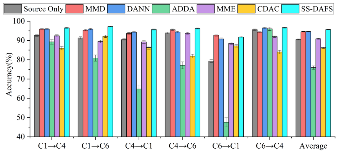
4.3. Case 1: Semi-Supervised Cross-Domain Classification Under Three-Shot Setting

Table 4. Classification accuracy (%) of different methods under the 3-shot semi-supervised domain adaptation setting. The best result for each transfer task is highlighted in bold.

Method	C1→C4	C1→C6	C4→C1	C4→C6	C6→C1	C6→C4	Average
Source Only	92.62 ± 0.52	91.35 ± 0.61	90.48 ± 0.68	93.92 ± 0.46	79.35 ± 0.79	95.58 ± 0.39	90.55 ± 0.26
MMD	95.88 ± 0.36	95.28 ± 0.42	93.65 ± 0.49	95.58 ± 0.38	92.72 ± 0.52	94.25 ± 0.34	94.56 ± 0.18
DANN	95.92 ± 0.39	95.88 ± 0.37	94.28 ± 0.45	94.32 ± 0.41	90.78 ± 0.58	96.52 ± 0.31	94.62 ± 0.19
ADDA	89.25 ± 1.18	80.85 ± 1.62	64.78 ± 2.05	77.12 ± 1.79	47.55 ± 2.38	96.02 ± 0.88	75.93 ± 0.92
MME	92.42 ± 0.55	89.48 ± 0.71	89.25 ± 0.78	93.72 ± 0.50	88.52 ± 0.66	91.98 ± 0.44	90.89 ± 0.28
CDAC	85.98 ± 0.88	92.15 ± 0.64	86.28 ± 0.82	81.85 ± 0.99	87.18 ± 0.74	83.98 ± 0.91	86.24 ± 0.36
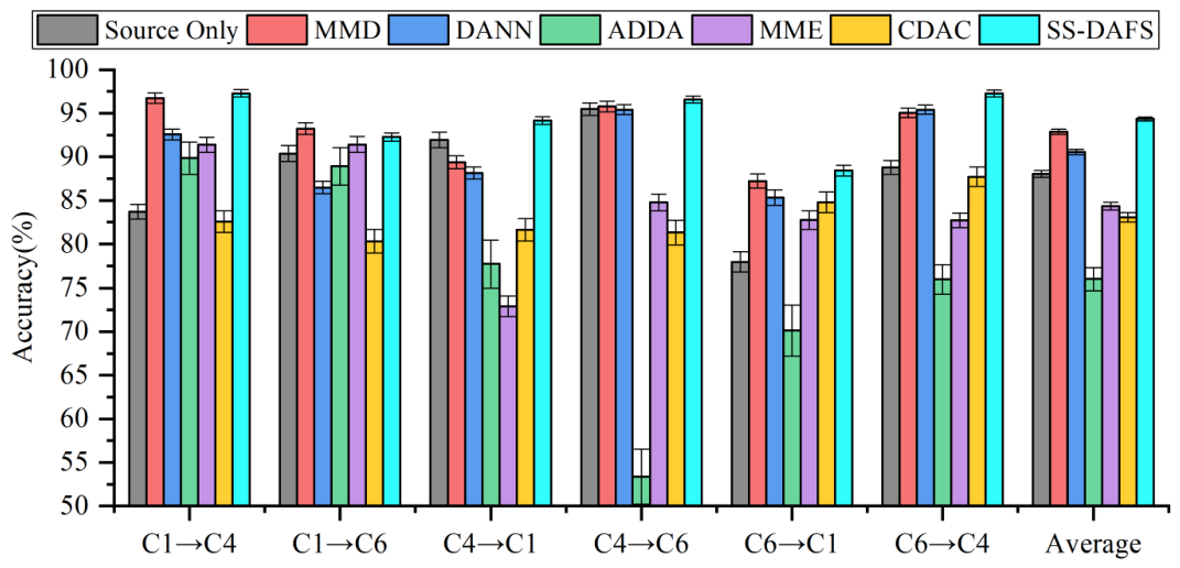
SS-DAFS	96.55 ± 0.26	97.22 ± 0.22	95.66 ± 0.29	96.22 ± 0.27	91.78 ± 0.41	96.64 ± 0.24	95.68 ± 0.13

and Figure 7 present the classification accuracy of different methods under the three-shot semi-supervised domain adaptation setting. Overall, the proposed SS-DAFS framework achieves the best average classification accuracy of $95.68\%\pm 0.13\%$, outperforming all comparison methods in most transfer tasks. Compared with the Source Only baseline ($90.55\%\pm 0.26\%$), all domain adaptation methods generally achieve improved performance, demonstrating the effectiveness of domain adaptation for cross-domain tool wear state classification.

Among the comparison methods, MMD and DANN achieve relatively competitive performance, with average accuracies of $94.56\%\pm 0.18\%$ and $94.62\%\pm 0.19\%$, respectively. These results indicate that discrepancy-based alignment and adversarial learning can effectively reduce the distribution discrepancy between different cutters. However, these methods mainly focus on global feature alignment and do not explicitly separate shared domain-invariant information from domain-specific characteristics, resulting in inferior performance compared with SS-DAFS. MME and CDAC achieve moderate performance, but their accuracies degrade noticeably on several transfer tasks, suggesting that entropy minimization and adaptive clustering strategies are insufficient to address the domain discrepancy caused by varying machining conditions.

The proposed SS-DAFS framework achieves the best performance in five out of six transfer tasks, including $97.22\%\pm 0.22\%$ accuracy on the C1→C6 task and $96.64\%\pm 0.24\%$ accuracy on the C6→C4 task. More importantly, it achieves the lowest average standard deviation of $0.13\%$ across all methods. The superior accuracy together with the minimal variance jointly demonstrate that the proposed feature separation strategy can effectively suppress domain-specific interference while preserving discriminative tool wear information, thereby improving both cross-domain generalization capability and training reproducibility under limited labeled target samples.

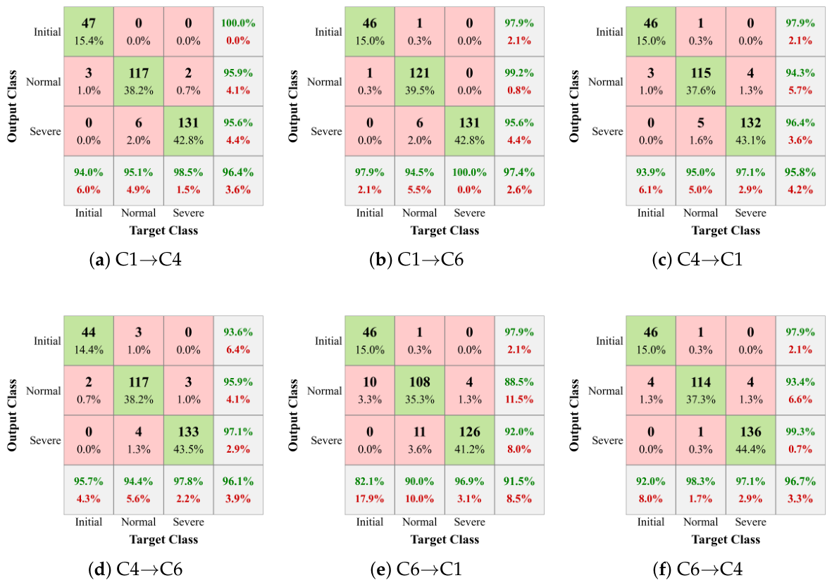
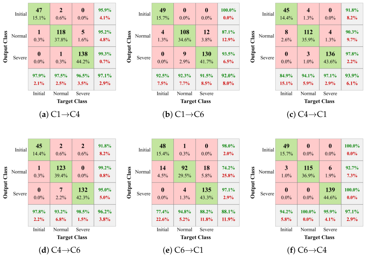
Figure 8 visualizes the classification results of the proposed SS-DAFS framework under the three-shot semi-supervised domain adaptation setting through confusion matrices. It can be observed that most samples are correctly classified along the diagonal region, indicating that the proposed framework achieves strong classification capability for different tool wear states under varying working conditions.

For the C1→C4, C1→C6, and C4→C1 tasks, the proposed method achieves highly accurate classification performance. In particular, the initial wear state achieves 100% classification accuracy in the C1→C4 task, while the severe wear state achieves 100% accuracy in the C1→C6 task. Moreover, the normal wear and severe wear states in most transfer tasks achieve classification accuracies above 94%, demonstrating that the proposed feature separation strategy can effectively preserve discriminative tool wear information under cross-domain scenarios.

Compared with the other transfer tasks, the C6→C1 task exhibits relatively lower classification performance. Specifically, the initial wear and normal wear states achieve classification accuracies of 82.1% and 88.5%, respectively, where several normal wear samples are misclassified into adjacent health states. This phenomenon may be caused by the relatively larger distribution discrepancy between the C6 and C1 cutters. Nevertheless, the overall classification accuracy still reaches 91.5%, indicating that the proposed SS-DAFS framework maintains robust cross-domain generalization capability even under challenging transfer conditions.

4.4. Case 2: Semi-Supervised Cross-Domain Classification Under One-Shot Setting

Table 5. Classification accuracy (%) of different methods under the 1-shot semi-supervised domain adaptation setting. The best result for each transfer task is highlighted in bold.

Method	C1→C4	C1→C6	C4→C1	C4→C6	C6→C1	C6→C4	Average
Source Only	83.72 ± 0.84	90.38 ± 0.91	91.95 ± 0.88	95.48 ± 0.72	77.95 ± 1.15	88.78 ± 0.78	88.04 ± 0.39
MMD	96.72 ± 0.58	93.25 ± 0.65	89.38 ± 0.74	95.78 ± 0.61	87.22 ± 0.82	95.05 ± 0.55	92.90 ± 0.29
DANN	92.58 ± 0.62	86.48 ± 0.71	88.15 ± 0.69	95.42 ± 0.58	85.32 ± 0.88	95.42 ± 0.52	90.56 ± 0.31
ADDA	89.85 ± 1.85	88.92 ± 2.15	77.72 ± 2.72	53.35 ± 3.15	70.12 ± 2.95	75.98 ± 1.68	75.99 ± 1.32
MME	91.38 ± 0.85	91.42 ± 0.92	72.92 ± 1.18	84.78 ± 0.95	82.75 ± 1.05	82.72 ± 0.82	84.33 ± 0.44
CDAC	82.58 ± 1.25	80.32 ± 1.35	81.62 ± 1.28	81.32 ± 1.42	84.78 ± 1.18	87.72 ± 1.12	83.06 ± 0.55
SS-DAFS	97.28 ± 0.42	92.28 ± 0.48	94.18 ± 0.45	96.58 ± 0.39	88.42 ± 0.62	97.28 ± 0.38	94.34 ± 0.21

and Figure 9 report the classification results under the more challenging one-shot setting, where only one labeled target sample per class is available. This setting is designed to stress-test the robustness of different methods when target-domain supervision approaches its practical limit. As expected, all methods suffer accuracy degradation compared with the three-shot setting, but the magnitude of degradation varies substantially. Taking the average accuracy drop as an indicator, CDAC, MME, and DANN degrade by $3.18$, $3.44$, and $4.06$ percentage points respectively, indicating that entropy minimization, adaptive clustering, and vanilla adversarial alignment are all sensitive to extreme supervision scarcity. A particularly revealing failure case concerns ADDA, which collapses on the C4→C6 task with only $53.35\%\pm 3.15\%$ accuracy. Such instability suggests that adversarial domain alignment, without explicit feature separation, cannot reliably extract discriminative representations when the target classifier has almost no supervised signal to anchor its decision boundaries.

Despite the extreme supervision scarcity, SS-DAFS not only maintains the highest average accuracy ($94.34\%\pm 0.21\%$) but also exhibits remarkably uniform stability across all transfer tasks: its per-task standard deviation never exceeds $0.62\%$. From the task-specific perspective, SS-DAFS also shows the narrowest performance gap between the easiest and hardest tasks, its accuracy ranges from $88.42\%$ to $97.28\%$, yielding a gap of only $8.86\%$, compared with $9.50\%$ for MMD and $10.10\%$ for DANN. The smaller gap indicates better cross-task consistency, further confirming that the proposed framework is robust to diverse cross-domain scenarios under extremely limited target supervision.

Figure 10 presents the confusion matrices of the proposed SS-DAFS framework across all six transfer tasks under the one-shot setting, where each matrix was evaluated on 312 target-domain samples. A joint inspection reveals that the normal wear class consistently contributes the largest share of misclassifications, whereas the initial and severe classes are recognized almost perfectly in most tasks.

It can be observed that direct confusions between the initial and severe classes are almost absent across all six tasks: the initial↔severe off-diagonal cells are exactly zero in five of the six matrices, and only in C4→C6 do two initial samples get misclassified as severe. In other words, virtually all errors occur between physically adjacent wear stages. This indicates that the shared feature space learned by SS-DAFS preserves the ordinal structure of the tool wear progression even under extreme supervision scarcity, suggesting that the proposed feature separation strategy prevents catastrophic feature collapse: domain-specific interference is absorbed by the private encoders, while the shared encoder retains representations that respect the underlying physical degradation trajectory.

Finally, the difficulty of adaptation varies markedly across transfer directions: C1→C4 and C6→C4 yield the cleanest matrices, whereas C6→C1 remains the hardest at $88.1\%$. Compared with the three-shot matrices in Figure 8, the framework exhibits graceful degradation. This indicates that the failure modes of SS-DAFS are predictable and physically rooted in the ambiguity of the normal wear stage, confirming that the feature separation strategy yields reliable and interpretable cross-domain representations even under single-sample supervision.

4.5. Ablation Study

To investigate the individual contribution of each component in the proposed SS-DAFS framework, an ablation study was conducted by progressively enabling four key components: the limited target supervision, the dual encoder with private encoders, the feature separation constraint realized by the difference loss, and the MMD-based distribution alignment. Four ablation models were constructed by adding exactly one component at each step, which are defined as follows:

• M1: The source-only baseline, in which a single shared encoder is trained with source classification only, without any target supervision or domain adaptation component.
• M2: M1 augmented with the limited target supervision, where one or three labeled target samples per class are used for supervised training.
• M3: M2 augmented with the private encoders, forming the dual encoder architecture that provides a dedicated pathway for domain-specific information.
• M4: M3 augmented with the difference loss, which explicitly decorrelates the shared and private representations to realize the feature separation principle.

Each model was evaluated on all six transfer directions under both the three-shot and one-shot settings, and every result was averaged over five independent runs. The results are reported in

Table 6. Ablation study under the 3-shot semi-supervised domain adaptation setting. Classification accuracy (%) of each model on all six transfer directions is reported. The best result for each transfer task is highlighted in bold.

Model	C1→C4	C1→C6	C4→C1	C4→C6	C6→C1	C6→C4	Average
M1	92.62 ± 0.52	91.35 ± 0.61	90.48 ± 0.68	93.92 ± 0.46	79.35 ± 0.79	95.58 ± 0.39	90.55 ± 0.26
M2	93.10 ± 0.47	93.20 ± 0.49	91.50 ± 0.58	94.05 ± 0.43	83.20 ± 0.71	95.40 ± 0.37	91.74 ± 0.24
M3	93.60 ± 0.41	92.80 ± 0.44	92.40 ± 0.49	94.90 ± 0.38	84.30 ± 0.60	95.80 ± 0.33	92.30 ± 0.21
M4	95.30 ± 0.33	95.60 ± 0.31	93.80 ± 0.39	95.20 ± 0.33	89.10 ± 0.50	96.00 ± 0.28	94.17 ± 0.17
SS-DAFS	96.55 ± 0.26	97.22 ± 0.22	95.66 ± 0.29	96.22 ± 0.27	91.78 ± 0.41	96.64 ± 0.24	95.68 ± 0.13

and

Table 7. Ablation study under the 1-shot semi-supervised domain adaptation setting. Classification accuracy (%) of each model on all six transfer directions is reported. The best result for each transfer task is highlighted in bold.

Model	C1→C4	C1→C6	C4→C1	C4→C6	C6→C1	C6→C4	Average
M1	83.72 ± 0.84	90.38 ± 0.91	91.95 ± 0.88	95.48 ± 0.72	77.95 ± 1.15	88.78 ± 0.78	88.04 ± 0.39
M2	87.90 ± 0.74	90.95 ± 0.79	92.30 ± 0.78	95.30 ± 0.65	81.20 ± 1.02	90.50 ± 0.69	89.69 ± 0.35
M3	88.80 ± 0.65	90.50 ± 0.70	93.00 ± 0.66	95.85 ± 0.56	82.10 ± 0.88	92.00 ± 0.58	90.38 ± 0.30
M4	93.60 ± 0.53	91.60 ± 0.59	93.40 ± 0.55	95.75 ± 0.48	86.20 ± 0.74	94.80 ± 0.48	92.56 ± 0.25
SS-DAFS	97.28 ± 0.42	92.28 ± 0.48	94.18 ± 0.45	96.58 ± 0.39	88.42 ± 0.62	97.28 ± 0.38	94.34 ± 0.21

, respectively.

As shown in Table 6 and Table 7, all four components contribute positively on average, yet their contributions are notably uneven, with the difference loss accounting for the single largest increment among the four steps. This uneven distribution can be understood from an optimization perspective. The target supervision provides a supervised anchor for the classifier, which explains the immediate gain of M2 over the baseline. The private encoders, in contrast, merely expand the representational capacity by introducing a separate branch; without any constraint governing what this branch should absorb, its potential remains largely unexploited, which is why M3 yields the smallest marginal improvement, increasing the average accuracy by only $0.56\%$ in the three-shot case.

The difference loss is what renders this dormant branch effective. Once it is enabled (M4), the shared and private representations are explicitly decorrelated, so that domain-specific factors are driven into the private branch while the shared branch is forced to encode purely wear-related information. This causal dependency, in which the separation constraint is required to unlock the capacity introduced by the private encoders, accounts for the most pronounced accuracy increment observed at the M3 to M4 transition, whereas M3 alone does not exhibit such an effect. These results confirm that the feature separation objective, rather than the target supervision or the distribution alignment, constitutes the methodological core of the proposed framework.

4.6. Visualization of Feature Separation and Cross-Domain Alignment

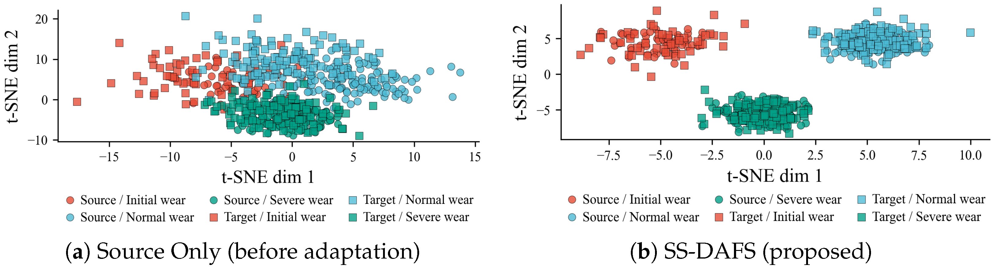
To provide visual evidence for the claim that feature separation improves cross-domain alignment, t-distributed Stochastic Neighbor Embedding (t-SNE) [40] was employed to project the learned shared feature representations into a two-dimensional space for a qualitative comparison. Figure 11 visualizes the shared feature embeddings before and after applying the proposed SS-DAFS framework on the representative C1→C4 transfer task under the one-shot setting. In each panel, the color of each point denotes the tool wear state (initial, normal, or severe), while the shape distinguishes the source domain (circle) from the target domain (square).

As shown in Figure 11a, without any domain adaptation strategy, the Source Only baseline exhibits a significant domain shift: source samples (circles) and target samples (squares) corresponding to the same wear state are largely separated in the feature space, especially for the initial wear and normal wear classes. This phenomenon indicates that features extracted from the pre-trained shared encoder still retain substantial domain-specific information induced by varying machining conditions, which hinders cross-domain generalization.

In contrast, Figure 11b demonstrates that the proposed SS-DAFS framework yields substantially improved cross-domain alignment. After joint optimization of the shared-private feature separation, MMD-based distribution alignment, and semi-supervised target classification, source and target samples of the same wear state exhibit much stronger overlap in the shared feature space. Meanwhile, samples from different wear states remain clearly separated, confirming that the feature separation strategy effectively preserves discriminative degradation-related information while suppressing domain-specific interference.

5. Conclusions

This paper proposed a SS-DAFS framework for intelligent condition monitoring of machining processes under cross-domain scenarios. The proposed framework adopts a dual encoder architecture that explicitly separates domain-invariant shared representations from domain-specific private representations and introduces an orthogonality-based feature separation constraint together with MMD-based domain alignment to improve cross-domain representation capability under limited labeled target samples. The effectiveness of the proposed method was validated through tool wear state classification tasks on the PHM2010 milling dataset. The main conclusions are summarized as follows:

• The proposed SS-DAFS framework effectively separates shared domain-invariant features and private domain-specific features, thereby enhancing feature representation capability for cross-domain condition monitoring tasks.
• The combination of difference loss and MMD-based similarity learning successfully reduces the distribution discrepancy between source and target domains while preserving discriminative degradation-related information.
• Comparative and ablation experiments on the PHM2010 dataset confirm the contribution of each proposed component. The proposed method achieves the best and most stable results across all transfer tasks.

Future work will focus on validating the proposed framework on additional real-world tool wear and condition monitoring datasets as more experimental data become available, since collecting and annotating high-quality machining data is a time-consuming process. Furthermore, domain generalization methods will be investigated to enable the proposed framework to learn domain-invariant representations solely from multiple source domains, thereby eliminating the dependence on target-domain data during training. In addition, the proposed framework will be extended to more complex machining scenarios to further improve its robustness and industrial applicability.