Trajectory Planning and Robustness Analysis for Mars Helicopters Under Uncertain Wind Fields

Abstract

Wind disturbances in the thin Martian are highly stochastic and spatially correlated, posing significant challenges to rotorcraft flight safety. Meanwhile, limited onboard computational resources make real-time safe trajectory planning difficult. This paper proposes a trajectory planning and analysis framework based on composite wind modeling and differential flatness theory. The proposed method decouples deterministic trajectory generation from stochastic robustness evaluation, enabling efficient trajectory planning in uncertain wind environments with planning-stage robustness evaluation. First, a composite wind model is constructed by combining multi-scale decomposition with Gaussian process regression, where a local kernel strategy is introduced to improve computational efficiency. Second, based on differential flatness theory and the MinCo method, a high-order polynomial trajectory is formulated. A multi-dimensional cost function is designed under wind field constraints to generate a nominal trajectory, incorporating trajectory smoothness, flight time, energy consumption, risk avoidance, and state feasibility. Finally, wind uncertainty is propagated via Monte Carlo sampling, and trajectory performance is quantitatively evaluated. Simulation results show the proposed method can generate safe, feasible, and risk-aware trajectories under the uncertain Martian wind conditions. Across all test scenarios, the mean terminal deviation, average deviation, and maximum deviation remain within 2.1%, 1.6%, and 3.6% of the trajectory length, respectively, indicating strong robustness in the evaluated scenarios.

1. Introduction

As a novel class of planetary exploration platforms, Mars helicopters [1,2] can overcome the terrain limitations of rovers while enabling large-scale, high-resolution, low-altitude reconnaissance missions. However, the Martian atmospheric environment is highly unique, with a density of approximately 1% of that at Earth’s sea level and wind disturbances exhibiting significant uncertainty, which critically affect flight safety [3]. Developing safe and reliable trajectory planning strategies under stochastic wind fields has therefore become a core challenge in Mars helicopter mission planning.

Currently, Mars helicopter trajectory planning primarily relies on an offline framework, where trajectories are pre-computed on the ground using a priori environmental models and subsequently uploaded to the vehicle for autonomous execution. NASA’s Ingenuity helicopter [4,5] has successfully completed multiple flights under this paradigm, demonstrating the feasibility of offline trajectory planning in the Martian environment. However, the performance of offline planning is highly dependent on the accuracy of a priori environmental models. Current trajectory planning relies on mesoscale wind field datasets [6,7] (e.g., MRAMS or Mars-GRAM) and modified Dryden stochastic turbulence models. However, their kilometer-scale resolution is insufficient to resolve the meter-scale local turbulence that critically governs load fluctuations in micro-rotorcraft flight dynamics. Agren et al. [8] demonstrated that low-frequency disturbances in the Martian atmosphere can significantly degrade the trajectory tracking accuracy of the Ingenuity helicopter, exceeding design-phase predictions, which highlights the limitations of current wind field models in characterizing environmental uncertainty.

The Mars Climate Database (MCD) [9,10] provides multi-scale wind statistics derived from global climate models and serves as the primary data source for current Mars mission planning. Based on this dataset, Piccione [11] developed a wind field model for Mars quadrotor simulations by superimposing uniformly distributed random perturbations and Gaussian white noise onto the mean wind obtained from the MCD. However, the model remains a macroscopic, spatiotemporally averaged representation and fails to capture transient fluctuations and small-scale turbulence in near-surface wind fields. Jackson [12] utilized flight data from Ingenuity (attitude and translational states) to infer near-ground wind speeds under specific aerodynamic assumptions, providing a new data source for modeling low-altitude Martian wind fields. However, this approach generally relies on steady-flight assumptions and simplified aerodynamic models. The resulting estimates reflect locally equivalent wind speeds and fail to capture the spatial correlation structure of the wind field.

Trajectory planning for Mars helicopters remains a challenging problem due to high-dimensional state variables, complex dynamic constraints, and significant environmental disturbances [13]. Existing approaches have gradually shifted from heuristic sampling-based algorithms, such as RRT* [14], toward numerical optimization frameworks. Sampling-based methods offer efficient global search capabilities for terrain avoidance [15] but typically rely on simplified kinematic models while neglecting rotor lift constraints and nonlinear aerodynamic effects in the thin Martian atmosphere, which may lead to actuator limit violations during execution. In contrast, optimization-based methods can generate dynamically feasible trajectories in the full state space by explicitly accounting for energy consumption and system constraints; however, their performance remains highly dependent on the accuracy of prior environmental models [16,17]. Differential flatness theory [18] provides an effective framework for dimensionality reduction in high-dimensional nonlinear trajectory planning for Mars helicopters. By parameterizing system states and control inputs as functions of flat outputs and their finite-order derivatives, the original optimization problem is transformed into a low-dimensional curve design problem, significantly reducing optimization complexity [19]. Duan [20] further extends the theory to a coupled helicopter-slung-load model for multi-agent cooperative systems, implicitly satisfying dynamic constraints while maintaining computational efficiency.

In practice, explicitly incorporating environmental uncertainty results in high-dimensional, strongly nonlinear, and non-convex optimization problems [21,22], substantially increasing computational complexity and making it difficult to achieve efficient and reliable solutions. Moreover, the limited onboard computational and energy resources of Mars helicopters [23] make real-time solutions of such stochastic optimization problems highly challenging during mission execution. Therefore, most existing studies adopt an offline planning and online execution framework to balance computational tractability and system robustness [24].

Recent advances have also highlighted the coupling between planning and tracking control for robustness under disturbances. Viadero-Monasteri et al. [25] proposed an integrated motion planning and robust output-feedback trajectory tracking framework for connected vehicles at unsignalized intersections. However, such terrestrial-oriented methods are not directly transferable to Mars helicopters due to the highly stochastic and spatially correlated wind fields in the thin Martian atmosphere. Unlike these approaches that address robustness primarily at the control stage, this paper decouples deterministic trajectory planning from statistical robustness evaluation via Monte Carlo simulation, enabling quantitative robustness assessment prior to deployment under limited onboard computational resources.

To enable quantitative robustness assessment under computational constraints, this paper proposes a trajectory planning framework integrating composite wind field modeling with differential flatness theory, while decoupling deterministic planning from statistical robustness evaluation. The main work of this paper is summarized as follows:

(1)

A composite wind field model combining multi-scale decomposition with Gaussian process regression and a local kernel strategy is constructed to characterize Martian atmospheric disturbances with computational efficiency.

(2)

Based on differential flatness theory and the MinCo method, high-order polynomial trajectories are generated under multi-source wind constraints, incorporating trajectory smoothness, flight time, energy consumption, risk avoidance, and state feasibility.

(3)

Monte Carlo-based statistical analysis is employed to quantitatively evaluate trajectory robustness under stochastic wind disturbances.

2. Composite Wind Field Modeling

To accurately characterize the spatial uncertainty structure of wind field disturbances in the thin Martian atmosphere at regional scales, a modeling framework is proposed by integrating multi-scale decomposition, Gaussian process regression, and local kernel modeling. Based on statistical data from the MCD, a composite wind field disturbance model with explicit spatial correlation is constructed.

2.1. Multi-Scale Disturbance Wind Field

Martian wind disturbances exhibit pronounced spatial scale separation, consisting of low-frequency, long-wavelength large-scale trends and high-frequency, short-wavelength local fluctuations. This multi-scale characteristic of Martian wind fields is represented in the MCD through large-scale trend components and small-scale turbulent components. Based on this decomposition, the disturbance wind $\delta v$ at point $x$ be expressed as

$$\delta v(x)=\delta v^{(L)}(x)+\delta v^{(S)}(x)$$

(1)

where $\delta v^{(L)}$ denotes the large-scale component with smooth spatial variation, and $\delta v^{(S)}$ denotes the small-scale component characterized by intense local fluctuations. Training data $D={\{(x_i,\delta v(x_i))\}}_{i=1}^N$ are directly obtained from the MCD, from which instantaneous wind fields under different regional, altitudinal, and seasonal conditions are extracted. After subtracting the corresponding background fields, disturbance samples are obtained for subsequent modeling. The large-scale and small-scale components are assumed to be statistically independent and are modeled separately before superposition.

2.2. Gaussian Process Modeling

Based on the multi-scale decomposition of Martian wind disturbances, Gaussian process regression is employed to construct composite models for the large-scale and small-scale components, respectively. This approach captures the spatial correlation structure of the disturbance field while providing probabilistic predictions and uncertainty quantification at arbitrary spatial locations, thereby enabling the generation of statistically consistent disturbance samples for subsequent analysis. Separate Gaussian process models are constructed for each component:

$$\delta v^{(L)}(x)\sim \mathcal{G}\mathcal{P}(0,k_L(x,x^{\prime }))$$

(2)

$$\delta v^{(S)}(x)\sim \mathcal{G}\mathcal{P}(0,k_S(x,x^{\prime }))$$

(3)

A zero-mean Gaussian process is adopted, where the prior assumes zero-mean wind disturbance at any spatial location, and the predictive mean is fully determined by observational data through spatial correlations. For any two points $x$ and $x^{\prime }$ in the wind field, the same squared exponential kernel is used for both the large-scale kernel $k_L$ and small-scale kernel $k_S$:

$$k_{\mathrm{L}}(x,x^{\prime })={\sigma }_{\mathrm{L}}^2\exp (-{\displaystyle \frac{1}{2}}{(x-x^{\prime })}^{{\rm T}}{L}_{\mathrm{L}}^{-2}(x-x^{\prime }))$$

(4)

$$k_{\mathrm{S}}(x,x^{\prime })={\sigma }_{\mathrm{S}}^2\exp (-{\displaystyle \frac{1}{2}}{(x-x^{\prime })}^{{\rm T}}{L}_{\mathrm{S}}^{-2}(x-x^{\prime }))$$

(5)

where $L_{\mathrm{L}}$ and $L_{\mathrm{S}}$ denote diagonal matrices representing spatial correlation length scales, characterizing long-range correlations and smooth variations for the large-scale component and rapid variations at local scales for the small-scale component, respectively. ${\sigma }_{\mathrm{L}}^2$ and ${\sigma }_{\mathrm{S}}^2$ represent the variances of the large-scale and small-scale Gaussian processes, respectively.

During model training, a total covariance matrix $K$ is constructed from the training samples for each disturbance component:

$$K=K_{\mathrm{L}}+K_{\mathrm{S}}+{\sigma }_n^{2}I$$

(6)

where $K_{\mathrm{L}}$ and $K_{\mathrm{S}}$ are the kernel matrices of all sample points for the large-scale and small-scale components, respectively; ${\sigma }_n$ is the observation noise variance used to fit the uncertainty in the disturbance data; and ${\rm I}$ is the identity matrix.

The hyperparameters in the kernel functions are optimized by maximizing the log-marginal likelihood [26] of the observed disturbance data:

$$-\log p(y|x,\theta )={\displaystyle \frac{1}{2}}{y}^T{K}^{-1}y+{\displaystyle \frac{1}{2}}\log \left|K\right|+const$$

(7)

where $p(y|x,\theta )$ denotes the marginal likelihood function and $\theta$ denotes all hyperparameters (e.g., length scales and signal variances). Specifically, we employ the L-BFGS optimizer with analytically derived likelihood derivatives for each hyperparameter. Critically, this optimization enforces a trade-off between data fidelity and model smoothness via the determinant term, which penalizes model complexity and prevents overfitting to measurement noise. The resulting wind field model provides both mean velocity predictions and predictive variance (uncertainty) estimates along candidate trajectories.

Therefore, for any prediction location $x^{*}$, the corresponding wind disturbance follows the predictive distribution:

$$\delta v(x^{*})\sim \mathcal{N}(\mu (x^{*}),{\sigma }^2(x^{*}))$$

(8)

where $\mu$ is the mean of the predicted disturbance and ${\sigma }^2$ is the variance of the predicted disturbance.

2.3. Local Kernel Modeling

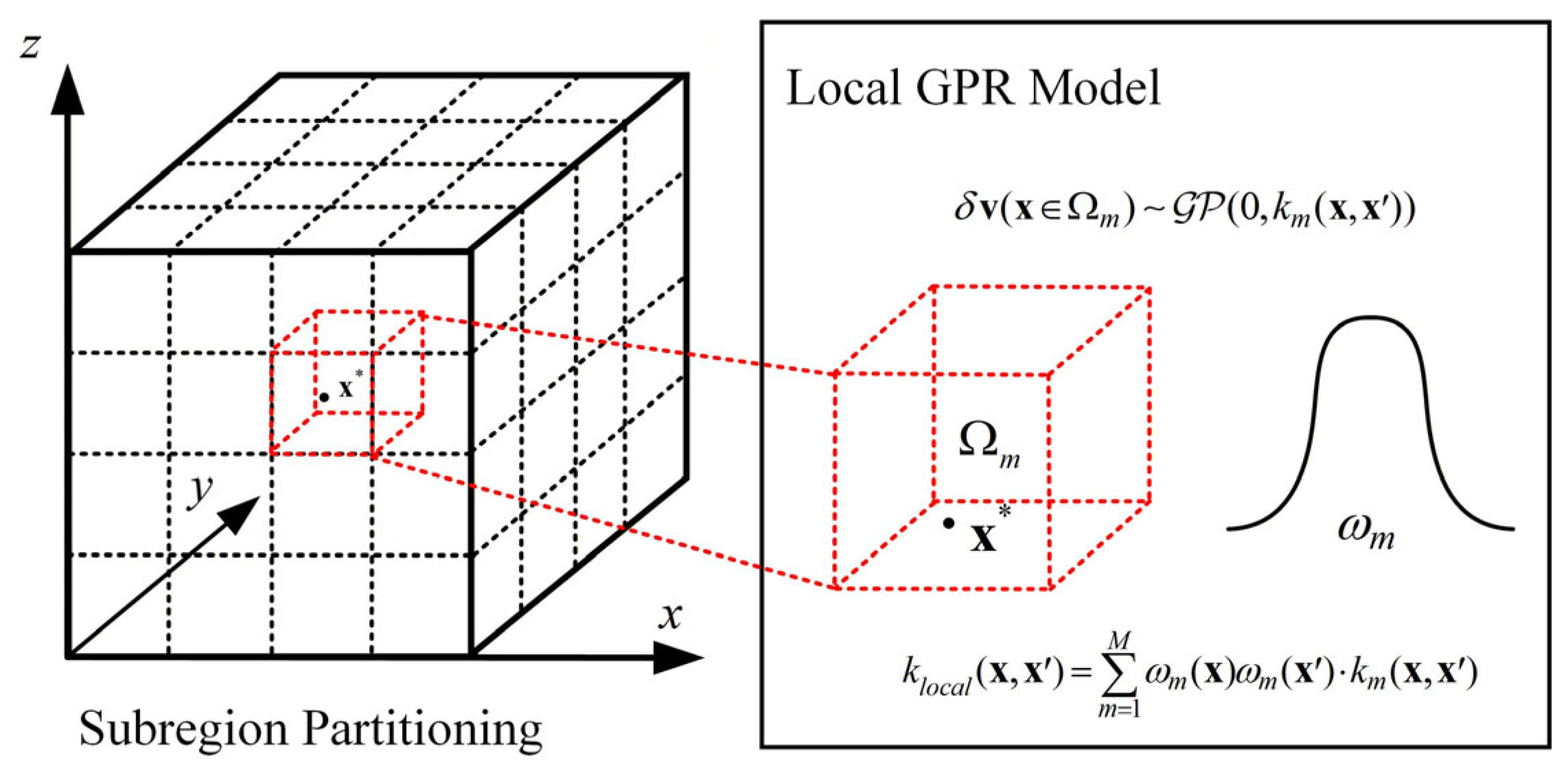
Directly constructing a global Gaussian process model on a large-scale three-dimensional grid requires forming a high-dimensional covariance matrix over all spatial points, resulting in a computational complexity of $\mathcal{O}(N^3)$ and a memory cost of $\mathcal{O}(N^2)$. To address this issue, a local kernel modeling mechanism [27] is introduced, which partitions the modeling domain into subdomains and trains local Gaussian process regression (GPR) models for each subdomain, thereby reducing computational complexity while improving the representation of local disturbance variations. Specifically, the modeling domain $\mathrm{\Omega }\in {ℝ}^3$ is partitioned into $M$ spatial subdomains $\left\{{\mathrm{\Omega }}_m\right\}$ according to spatial location, and an independent GPR submodel is trained within each subdomain, each equipped with its own set of kernel hyperparameters $k_m$:

$$\delta v(x\in {\mathrm{\Omega }}_m)\sim \mathcal{G}\mathcal{P}(0,k_m(x,x^{\prime }))$$

(9)

The local kernel function takes the following form:

$$k_m(x,x^{\prime })={\sigma }_m^2\exp (-{\displaystyle \frac{1}{2}}{(x-x^{\prime })}^{{\rm T}}{L}_m^{-2}(x-x^{\prime }))$$

(10)

Meanwhile, to eliminate discontinuities in predictions across subdomain boundaries, a kernel-weighted fusion strategy is adopted to construct a globally continuous kernel function $k_{local}$:

$$k_{local}(x,x^{\prime })={\displaystyle {\displaystyle \sum _{m=1}^M}{\omega }_m(x)}{\omega }_m(x^{\prime })\cdot k_m(x,x^{\prime })$$

(11)

where ${\omega }_m(x)\in [0,1]$ is the normalized spatial membership weight, reflecting the contribution of location to each subdomain and satisfying ${\displaystyle {\sum }_m{\omega }_m(x)}=1$. The strategy enables smooth transitions between subdomain kernel functions and yields a probabilistic wind disturbance model to represent non-stationary characteristics, as illustrated in Figure 1.

Figure 1. Frame for Local Kernel Modeling.

2.4. Transient Wind Disturbance Modeling

To capture transient wind fluctuations under strong convective conditions, a stochastic disturbance is introduced into the background wind to construct a non-stationary probabilistic wind speed model. Specifically, the instantaneous wind speed $v$ is expressed as the superposition of the background wind and a random disturbance term:

$$v(x)=v_{\mathrm{mean}}(x)+\delta v(x)+\delta \xi (x)$$

(12)

where $v_{\mathrm{mean}}$ denotes the mean wind speed provided by the MCD, and $\xi$ is a zero-mean Gaussian random process that describes terrain- and convection-induced transient wind disturbances. The disturbance amplitude $\delta$ is sampled according to a prescribed probability distribution, thereby constructing a wind field model with non-stationary characteristics.

This modeling approach preserves the consistency of the background wind while introducing low-probability, high-intensity disturbances, thereby enhancing the representation of extreme scenarios within the wind field model. Consequently, a more stringent and representative environment is provided for the robustness evaluation of subsequent trajectory planning methods.

3. Differential Flatness-Based Trajectory Planning Method

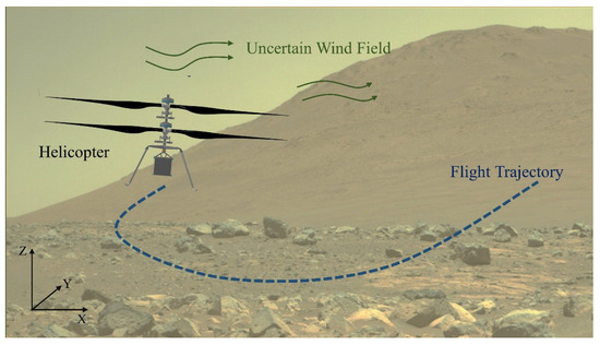
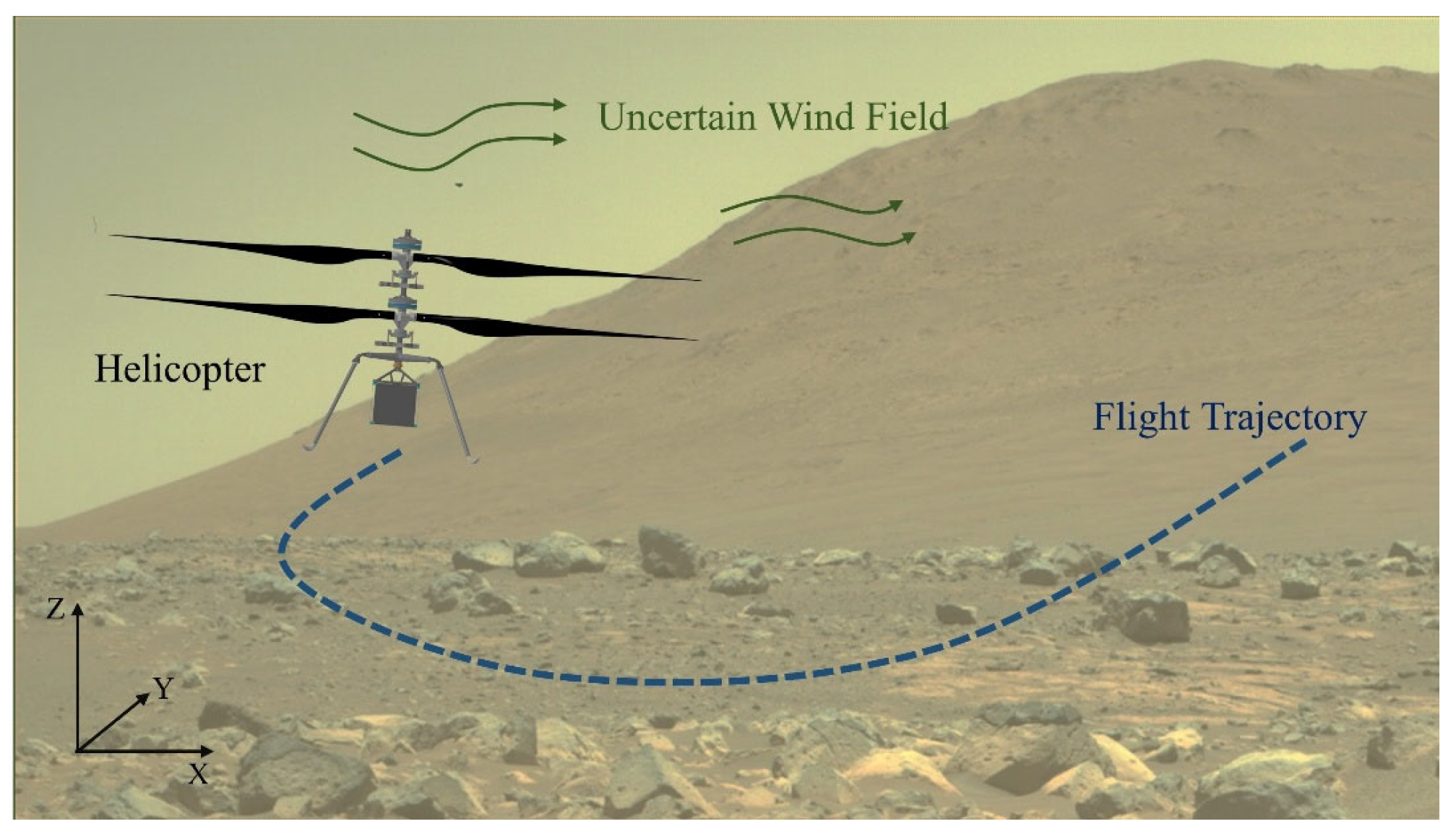
To address multi-objective constraints and complex environmental influences in Mars helicopter trajectory planning, as illustrated in Figure 2, a differential flatness-based framework is adopted to reformulate trajectory generation as a spatiotemporally coupled parameterization problem of flat outputs. Using the MinCo method [28], the trajectory is parameterized as a high-order polynomial. A multi-dimensional cost function is then formulated, incorporating energy minimization, time optimization, trajectory smoothness, risk avoidance, and flight state feasibility, to establish a trajectory optimization model tailored to the Martian environment. On this basis, a Monte Carlo-based framework is employed to generate wind disturbance samples for trajectory robustness evaluation.

Figure 2. Mars helicopter trajectory planning under uncertain wind field disturbances.

3.1. Differential Flatness Properties of the Mars Helicopter

This section focuses on a Mars coaxial helicopter and establishes its differential flatness formulation under a simplified dynamic model. To reduce model complexity, a quasi-static approximation is adopted, assuming small attitude variations during flight and rapid convergence of dynamic responses, while neglecting high-frequency transient effects and attitude coupling terms. The coaxial helicopter is modeled as a rigid-body system with translational degrees of freedom. The force model includes wind field disturbances and gravity, with the thrust direction assumed to remain aligned with the body $z$ axis. Lateral and backward rotor forces, as well as aerodynamic forces and moments generated by the fuselage during flight, are neglected.

The helicopter state vector is defined as $x_{\mathrm{H}}={[P,R,V,\omega ]}^T$, where $P\in {ℝ}^3$ denotes the position vector in the Mars-fixed frame, $R\in S{O}^3$ denotes the attitude transformation matrix induced by the fuselage orientation, $V\in {ℝ}^3$ denotes the translational velocity expressed in the Mars-fixed frame, and $\omega \in {ℝ}^3$ denotes the body angular velocity. The control input is defined as $u=\{f,\tau \}$, in which $f\in {ℝ}_{\ge 0}$ corresponds to the total rotor thrust and $\tau \in {ℝ}^3$ denotes the aerodynamic torque generated by the rotor with respect to the vehicle center in the body-fixed frame. Therefore, the dynamic equations of the Martian helicopter can be expressed as follows:

$$\left\{\begin{array}{c}\dot{P}=V\\ m\dot{V}=-mg{e}_3+R\cdot f{e}_3-RD{R}^T\sigma (‖V_{ref}‖)\cdot V_{\mathrm{ref}}\\ \dot{R}=R\omega \\ M\dot{\omega }=\tau -\omega \cdot M\omega -A(\omega )-B(R^T{V}_{\mathrm{ref}})\end{array}\right.$$

(13)

where $m$ denotes the helicopter mass, $e_3={[0,0,1]}^T$ is the direction vector, $g$ denotes the gravitational acceleration on Mars, $M$ denotes the inertia tensor matrix of the vehicle with respect to the body-fixed frame centered at the center of mass, and $D$ is the aerodynamic drag coefficient. Furthermore, $\sigma (x)=1+C_{p}x$ denotes the nonlinear translational acceleration term resulting from the combined effects of the linear damping and the parasite drag [29], $A$ represents the drag-induced moment caused by attitude variations, and $B$ denotes the unbalanced aerodynamic moment generated by the relative wind velocity acting on the fuselage.

Furthermore, nonlinear aerodynamic drag effects are explicitly incorporated into the dynamic model to accurately capture the disturbances induced by wind fields in the thin Martian atmosphere. Specifically, the reference velocity vector $V_{\mathrm{ref}}$ of the vehicle relative to the local wind field is defined as follows:

$$V_{\mathrm{ref}}=V-v_{\mathrm{mean}}$$

(14)

Since disturbance wind fields cannot be accurately represented by finite-order derivatives, stochastic wind disturbances are not explicitly incorporated into the dynamic equations. Instead, wind uncertainty is evaluated after trajectory optimization through Monte Carlo simulations.

In this study, the helicopter position $P$ and yaw angle $\psi$ are selected as the flat outputs of the system, denoted by $z=\{P,\psi \}$, where $r^{[s]}$ is defined as the stacked vector $(r,\dot{r},\dots ,r^{(s)})$ of derivatives up to the $s^{th}$ order. Therefore, the differential flatness transformation establishes a mapping $\mathrm{\Psi }$ in which the system states and control inputs are uniquely determined by the flat outputs and their finite-order derivatives.

$$(x_H,u)=\mathrm{\Psi }(P^{[s]},{\psi }^{[s]})$$

(15)

Accordingly, the dynamic model of the Mars helicopter under wind conditions is established. Since the mapping relationships among flat outputs, system states, and control inputs have been extensively derived in prior studies [30,31], they are omitted here.

3.2. Risk Region Modeling

In the Martian wind environment with significant disturbances, effective identification and avoidance of potential high-risk regions are essential for improving rotorcraft mission safety. To this end, a risk region identification criterion based on the multi-scale statistical characteristics of the wind field is proposed, jointly considering wind intensity, disturbance magnitude, spatial gradient variation, and local turbulence characteristics.

(a)

Maximum Wind Speed and Disturbance Intensity Criterion

Wind velocity is one of the primary external disturbances acting on the vehicle during flight, and its magnitude directly affects flight controllability and maneuverability. The disturbance standard deviation reflects turbulence intensity and characterizes the unsteady properties of the wind field. Therefore, wind speed threshold $v_{th}$ and disturbance standard deviation threshold ${\sigma }_{th}$ are introduced to define potential risk regions ${\mathcal{A}}_1$ as follows:

$${\mathcal{A}}_1=\left\{x|‖v‖\ge v_{th}\right\}\cup \left\{x|‖\delta v‖\ge {\sigma }_{th}\right\}$$

(16)

(b)

Wind Speed Spatial Gradient Criterion

The spatial gradient of wind speed is used to identify regions with abrupt wind variations that may induce flight control difficulties. It is defined as follows:

$$‖\nabla v‖=\sqrt{{\left({\displaystyle \frac{\partial ‖v‖}{\partial x}}\right)}^2+{\left({\displaystyle \frac{\partial ‖v‖}{\partial y}}\right)}^2+{\left({\displaystyle \frac{\partial ‖v‖}{\partial z}}\right)}^2}$$

(17)

where regions where the wind speed gradient exceeds the prescribed threshold $\nabla v_{th}$ are identified as risk regions ${\mathcal{A}}_2$, defined as follows:

$${\mathcal{A}}_2=\left\{x|‖\nabla v‖\ge \nabla v_{th}\right\}$$

(18)

(c)

Turbulence Intensity Criterion

Turbulence intensity $TI$ is used to quantify the relative magnitude of wind fluctuations with respect to the mean flow speed and is defined as follows:

$$TI={\displaystyle \frac{\delta v}{‖v‖+\xi }}$$

(19)

where $\xi$ denotes a small positive constant introduced to avoid division by zero. Regions with high turbulence intensity indicate that wind disturbances dominate the local flow dynamics. Given the turbulence intensity threshold $T{I}_{th}$, the corresponding risk regions ${\mathcal{A}}_3$ are defined as follows:

$${\mathcal{A}}_3=\left\{x|TI\ge T{I}_{th}\right\}$$

(20)

(d)

Integrated Risk Region

Since wind disturbances exhibit continuous spatial variations, representing hazardous regions using binary obstacles cannot accurately characterize the environmental risk. Therefore, a continuous wind risk field is constructed.

The final risk region $\mathcal{A}$ is determined by the union of all sub-criteria, which can be expressed as follows:

$$\mathcal{A}={\mathcal{A}}_1+{\mathcal{A}}_2+{\mathcal{A}}_3$$

(21)

This formulation enables the optimizer to evaluate the environmental risk continuously along the trajectory. All spatial points satisfying any threshold-exceeding criterion are regarded as potential high-risk regions and should be properly avoided during the trajectory planning process.

It should be emphasized that the risk region identification in this study is not intended for mission-level go/no-go decisions, which are typically made during pre-flight environmental assessment. Instead, it serves as a local planning constraint to avoid relatively high-risk subregions within an already admissible flight domain. The threshold-based criteria are designed to be conservative, ensuring that the planned trajectory maintains a safe margin from potentially hazardous wind conditions.

3.3. MinCo-Based Spatiotemporal Trajectory Deformation

The MinCo method employs polynomial parameterization over multiple trajectory segments and minimizes the norm of high-order derivatives as the cost function, thereby enhancing trajectory smoothness and reducing control effort. To generate dynamically feasible trajectories with sufficient smoothness, each trajectory segment is parameterized using a high-order polynomial within the MinCo framework. Assume that the entire flight trajectory consists of $M$ segments, where the $i^{th}$ segment $p_i$ is represented by an $N=2s-1$ order polynomial over the time interval $[t_{i-1},t_i]$ as follows:

$$p_i(t)=c_i^T\cdot \beta (t-t_{i-1}),t\in [t_{i-1},t_i]$$

(22)

where $\beta (x)={(1,x,\dots ,x^N)}^T$ denotes the polynomial basis, and $c_i\in {ℝ}^{2s\times m}$ denotes the coefficient matrix of the polynomial. The polynomial coefficients are determined by satisfying the boundary and continuity constraints. Accordingly, the complete flight trajectory can be expressed as follows:

$${\mathrm{\Gamma }}_{\mathrm{MINCO}}=\{p(t):[0,T_{\Sigma }]\mapsto {ℝ}^m|c=\mathit{C}(q,T),q\in {ℝ}^{m(M-1)},T\in {ℝ}^M\}$$

(23)

where $c={(c_1^T,\dots ,c_M^T)}^T$, $q=(q_1,\dots ,q_{M-1})$ denote the intermediate waypoints of the differentially flat trajectory, with $T={(T_1,\dots ,T_M)}^{\mathrm{T}}$ satisfying $T_i=t_i-t_{i-1}$. In addition, $T_{\Sigma }={\displaystyle {\sum }_{i=1}^M{T}_i}$ represents the total flight time.

Here, $D_0$, $D_M$ and $D_i$ are defined as the state derivatives specified by the boundary conditions and intermediate constraints of the trajectory. Accordingly, the trajectory at time $t_i$ satisfies:

$$(E_{\mathrm{i}}{F}_{\mathrm{i}})\left(\begin{array}{c}{c}_{\mathrm{i}}\\ c_{\mathrm{i}+1}\end{array}\right)=\left(\begin{array}{c}{D}_{\mathrm{i}}\\ 0\end{array}\right)$$

(24)

where $E$ and $F$ denote the corresponding coefficient matrices. By incorporating all boundary conditions and continuity constraints into the polynomial parameterization, the trajectory coefficients can be determined by solving the following linear equation system:

$$\mathit{N}\mathit{c}=\mathit{b}$$

(25)

where $N\in {ℝ}^{2Ms\times 2Ms}$ denotes the assembled block coefficient matrix formed by the boundary and continuity constraints, and $b\in {ℝ}^{2Ms\times m}$ denotes the corresponding right-hand-side coefficient vector. Their detailed formulations are given in Equation (26).

$$N=\left(\begin{array}{ccccc}{F}_0& 0& 0& \dots & 0\\ E_1& F_1& 0& \dots & 0\\ 0& E_2& F_2& \dots & 0\\ ⋮& ⋮& ⋮& \ddots & ⋮\\ 0& 0& 0& \dots & F_{M-1}\\ 0& 0& 0& \dots & E_M\end{array}\right) b=\left(\begin{array}{c}{D}_0\\ D_1\\ 0\\ ⋮\\ D_{M-1}\\ 0\\ D_M\end{array}\right)$$

(26)

Based on the above formulation, a MinCo-based trajectory parameterization framework for the Martian helicopter is established in this study. By solving the above equations, the polynomial coefficient matrix $\mathit{c}$ can be obtained, thereby fully characterizing the continuous spatial trajectory of the vehicle over the time domain. Considering a twice-differentiable cost function $\mathcal{K}(\mathit{c},\mathit{T})$, the corresponding objective function for the MinCo trajectory is formulated as follows:

$$\mathcal{W}(q,T)=\mathcal{K}(c(q,T),T)$$

(27)

To optimize the above cost function, the gradients of $\mathcal{W}$ with respect to $q$ and $T$, denoted by $\partial \mathcal{W}/\partial q$ and $\partial \mathcal{W}/\partial \mathit{T}$, need to be computed. For computational convenience, Equation (24) can be reformulated as follows:

$$N(\mathit{T})c(q,T)=b(q)$$

(28)

By differentiating both sides of the equation with respect to $q_{i,j}$ and $T$, the following expressions can be obtained:

$${\displaystyle \frac{\partial c}{\partial q_{i,j}}}=N^{-1}{\displaystyle \frac{\partial b}{\partial q_{i,j}}}$$

(29)

$${\displaystyle \frac{\partial N}{\partial T_i}}+N{\displaystyle \frac{\partial c}{\partial T_i}}=0$$

(30)

Accordingly, the following results can be derived:

$${\displaystyle \frac{\partial \mathcal{W}}{\partial q_{i,j}}}=Tr\left\{{\left({\displaystyle \frac{\partial b}{\partial q_{i,j}}}\right)}^{\mathrm{T}}\left(N^{-\mathrm{T}}{\displaystyle \frac{\partial \mathcal{K}}{\partial c}}\right)\right\}$$

(31)

$${\displaystyle \frac{\partial \mathcal{W}}{\partial T_i}}={\displaystyle \frac{\partial \mathcal{K}}{\partial T_i}}-Tr\left\{\left(N^{-\mathrm{T}}{\displaystyle \frac{\partial \mathcal{K}}{\partial c}}\right){\displaystyle \frac{\partial N}{\partial T_i}}c\right\}$$

(32)

The trajectory cost function is optimized through the spatiotemporal deformation mechanism of MinCo, yielding an implicit optimization formulation. Based on the practical flight constraints and mission requirements of Mars helicopter missions, a physically interpretable cost function and constraint set are constructed to establish a comprehensive trajectory optimization model balancing energy consumption, flight time, feasibility, and safety.

3.4. Multi-Objective Trajectory Cost Function

To ensure favorable dynamic performance, environmental adaptability, and mission feasibility, a trajectory optimization problem with multiple objectives and constraints is formulated within the MinCo spatiotemporal parameterization framework. The overall objective function is given as follows:

$$\underset{(c,T)}{\min }\mathcal{K}(c(q,T),T)=\lambda {[J_s,J_t,J_r,J_f,J_e]}^{\mathrm{T}}$$

(33)

where $J_s$ denotes the trajectory smoothness penalty term, $J_t$ represents the minimum flight time penalty term, $J_r$ denotes the risk region penalty term, $J_f$ represents the flight state constraint penalty term, and $J_e$ denotes the minimum flight energy term. $\lambda =\left[{\lambda }_s,{\lambda }_t,{\lambda }_r,{\lambda }_f,{\lambda }_e\right]\in {ℝ}^5$ are the corresponding weighting coefficients for each penalty term. Each term corresponds to a specific optimization objective, and the weighting coefficients determine their relative importance.

(a)

Trajectory Smoothness Penalty

To ensure sufficient smoothness and dynamic continuity of the trajectory, the integral of the squared fourth-order derivative is adopted as the smoothness penalty term in this study:

$$\begin{array}{l}{J}_s(c_i,T_i)={\displaystyle {\int }_0^{T_i}{p}_i^{(4)}{\left(t\right)}^{\mathrm{T}}{p}_i^{(4)}\left(t\right)dt}\\ =Tr\left\{c_i^{\mathrm{T}}\left({\displaystyle {\int }_{t_{i-1}}^{T_i}{\beta }^{(4)}(t){\beta }^{(4)}{(t)}^{\mathrm{T}}dt}\right)c_i\right\}\end{array}$$

(34)

Let $R(t)={\beta }^{(4)}(t){\beta }^{(4)}{(t)}^{\mathrm{T}}$ and $Q(\tau )={\displaystyle {\int }_0^{\tau }R(t)dt}$. Then, by differentiating $J_s$ with respect to $c_i$ and $T_i$, the following expressions can be obtained:

$${\displaystyle \frac{\partial J_s}{\partial c_i}}=2Q(T_i)c_i$$

(35)

$${\displaystyle \frac{\partial J_s}{\partial T_i}}=Tr\left\{c_i^{\mathrm{T}}R(T_i)c_i\right\}$$

(36)

(b)

Minimum Flight Time Penalty

To improve mission efficiency and system responsiveness, the total flight duration is incorporated as a penalty term in the cost function:

$$J_t=T_{\Sigma }$$

(37)

By differentiating $J_t$ with respect to $c_i$ and $T_i$, the corresponding gradients can be obtained as $\partial J_t/\partial c_i=0$ and $\partial J_t/\partial T_i=1$, respectively.

(c)

Risk Avoidance Penalty

To enhance trajectory adaptability to uncertain wind fields, a minimum safety distance $l_{th}$ is introduced to constrain the minimum separation between trajectory points and risk regions. When the trajectory approaches or enters high-risk regions, a weighted penalty term is imposed in the cost function.

Let $P_{i,j}$ denote the helicopter position at the $j^{th}$ sampling point corresponding to the differential flat output of the $i^{th}$ trajectory segment. Then, the risk avoidance penalty term can be formulated as follows:

$$J_r={\displaystyle {\displaystyle \sum _{i=1}^M}\frac{T_i}{k_i}}{\displaystyle {\displaystyle \sum _{j=0}^{k_i}}{\overline{\omega }}_j\max {\left({\phi }_{r.i.j},0\right)}^3}$$

(38)

where $\left({\overline{\omega }}_0,{\overline{\omega }}_1,\dots ,{\overline{\omega }}_{k_i-1},{\overline{\omega }}_{k_i}\right)=\left(0.5,1,\dots ,1,0.5\right)$ denotes the quadrature coefficient following the trapezoidal rule for numerical integration, and ${\phi }_{r.v.i.j}$ is used to penalize violations of the minimum safety distance between the helicopter and the wind risk region:

$${\phi }_{r.i.j}=\left\{\begin{array}{cc}{l}_{th}-d{L}_{i.j}& \mathrm{if}d{L}_{i.j}<l_{th}\\ 0& \mathrm{if}d{L}_{i.j}\ge l_{th}\end{array}\right.$$

(39)

where $d{L}_{i.j}$ denotes the minimum distance between the helicopter position and the center of the nearest risk region, which is defined as follows:

$$d{L}_{i.j}=\underset{P_r\in \mathcal{A}}{\min }‖P_{i,j}-P_r‖$$

(40)

When $d{L}_{i.j}<l_{th}$ is satisfied, the derivatives of $J_r$ with respect to $c_i$ and $T_i$ can be obtained as follows:

$$\left\{\begin{array}{l}{\displaystyle \frac{\partial J_r}{\partial c_i}}=-{\displaystyle \frac{\partial J_r}{\partial {\phi }_{r.i.j}}}\beta (t){(\nabla d{L}_{i.j})}^T\\ {\displaystyle \frac{\partial J_r}{\partial T_i}}={\displaystyle \frac{J_r}{T_i}}-{\displaystyle \frac{\partial J_r}{\partial {\phi }_{r.i.j}}}{\displaystyle \frac{\partial t}{\partial T}}{(\nabla d{L}_{i.j})}^T\dot{P}(t)\end{array}\right.$$

(41)

where $t=j/k_i{T}_i$ and $\partial t/\partial T_i=j/k_i$, $\nabla d{L}_{i.j}$ denotes the distance gradients.

(d)

Flight State Constraint Penalty

To ensure the physical feasibility of the planned trajectory, a flight-state constraint penalty term is introduced to enforce allowable limits on key helicopter states, including velocity, acceleration, and maximum rotor thrust. Taking the maximum velocity constraint $V_{th}$ as an example, the corresponding penalty function is constructed as follows:

$$J_f={\displaystyle {\displaystyle \sum _{i=1}^M}\frac{T_i}{k_i}}{\displaystyle {\displaystyle \sum _{j=0}^{k_i}}{\overline{\omega }}_j\max {\left({\phi }_{f.v.i.j},0\right)}^3}$$

(42)

where ${\phi }_{f.v.i.j}$ is used to quantify the extent to which the helicopter flight velocity exceeds the prescribed maximum velocity limit, expressed as follows:

$${\phi }_{f.v.i.j}=\left\{\begin{array}{cc}{‖V_{i,j}‖}^2-V_{th}^2& \mathrm{if}‖V_{i,j}‖>V_{th}\\ 0& \mathrm{if}‖V_{i,j}‖\le V_{th}\end{array}\right.$$

(43)

where $V_{i,j}$ denote the helicopter velocity at the $j^{th}$ sampling point of the $i^{th}$ trajectory segment. When $‖V_{i,j}‖>V_{th}$ is satisfied, the derivatives of $J_f$ with respect to $c_i$ and $T_i$ can be obtained as follows:

$$\left\{\begin{array}{l}{\displaystyle \frac{\partial J_f}{\partial c_i}}={\displaystyle \frac{\partial J_f}{\partial {\phi }_{f.v.i.j}}}\cdot 2\dot{\beta }(t)V_{i.j}\\ {\displaystyle \frac{\partial J_f}{\partial T_i}}={\displaystyle \frac{J_f}{T_i}}+{\displaystyle \frac{\partial J_f}{\partial {\phi }_{f.v.i.j}}}{\displaystyle \frac{\partial t}{\partial T_i}}\cdot 2V_{i.j}^{\mathrm{T}}{\dot{V}}_{i.j}(t)\end{array}\right.$$

(44)

Similar to the maximum flight velocity constraint penalty term, the penalty functions for the maximum acceleration and rotor thrust constraints, along with their corresponding derivatives, can be derived analogously.

(e)

Minimum Flight Energy Penalty

Under the low-density Martian atmosphere, rotor power consumption is dominated by induced power, whereas profile and parasitic drag power are significantly reduced and contribute negligibly to speed-dependent energy variation [32]. Moreover, typical mission trajectories mainly involve low-speed maneuvers and hovering, during which induced inflow and load-dependent variations dominate energy consumption. Accordingly, the flight energy cost is defined as the time integral of induced power, capturing the dominant energy expenditure while avoiding unnecessary modeling complexity.

The induced power $H$ of the rotor can be expressed as follows:

$$H=f^{3/2}/\sqrt{2\rho S}$$

(45)

where $\rho$ denotes the Martian atmospheric density, and $S$ represents the rotor disk area. Therefore, the minimum flight energy penalty term can be formulated as follows:

$$J_e={\displaystyle {\displaystyle \sum _{i=1}^M}\frac{T_i}{k_i}}{\displaystyle {\displaystyle \sum _{j=0}^{k_i}}{\overline{\omega }}_j{H}_{i,j}}$$

(46)

Then, the derivatives of $J_e$ with respect to $c_i$ and $T_i$ are obtained as follows:

$$\left\{\begin{array}{l}{\displaystyle \frac{\partial J_e}{\partial c_i}}={\displaystyle \frac{3}{2}}{\displaystyle \frac{J_e}{\partial H_{i,j}}}{\displaystyle \frac{f^{1/2}}{\sqrt{2\rho S}}}((\sigma (‖V_{\mathrm{ref}}‖)c+C_p{\displaystyle \frac{c^T{V}_{\mathrm{ref}}}{‖V_{\mathrm{ref}}‖}}{V}_{\mathrm{ref}})\dot{\beta }(t)+m{e}_3^T{R}^T\ddot{\beta }(t))\\ {\displaystyle \frac{\partial J_e}{\partial T_i}}={\displaystyle \frac{J_e}{T_i}}+{\displaystyle \frac{3}{2}}{\displaystyle \frac{\partial J_e}{\partial H_{i,j}}}{\displaystyle \frac{f^{1/2}}{\sqrt{2\rho S}}}{\displaystyle \frac{\partial f}{\partial t}}{\displaystyle \frac{\partial t}{\partial T}}\end{array}\right.$$

(47)

(f)

Time Constraint Penalty

For each segment of the differentially flat output trajectory, the corresponding time variable is required to satisfy $T_i>0$. This constraint can be handled via the following diffeomorphic mapping:

$$T_i=e^{{\tau }_i}$$

(48)

For ${\tau }_i\in ℝ$, the condition $T_i>0$ is satisfied. Therefore, $T_i$ can be optimized by optimizing ${\tau }_i$:

$$\partial J/\partial {\tau }_i=(\partial J/\partial T_i)e^{{\tau }_i}$$

(49)

A unified weighted multi-objective cost function is formulated to simultaneously account for energy consumption, flight time, trajectory smoothness, risk avoidance, and flight state feasibility. Since the MinCo-based optimization process is sensitive to the initial guess, the Rapidly-exploring Random Tree (RRT) algorithm is introduced to generate the initial trajectory, thereby improving optimization stability and computational reliability.

3.5. Trajectory Robustness Evaluation

Based on the Gaussian process probabilistic wind model, a Monte Carlo simulation framework [33] is constructed for robustness evaluation. By performing dynamic simulations of the planned trajectory under multiple statistically independent perturbed wind fields, the influence of wind uncertainty on key performance metrics, including trajectory deviation and safety margin, is quantitatively assessed. This framework provides a statistical basis for robustness analysis and iterative refinement of planner parameters.

A discrete dynamic model is adopted for state propagation to accurately describe the cumulative effect of wind field disturbances on the trajectory. The motion of the helicopter under the influence of the wind field satisfies

$${\mathit{v}}_{k+1}={\mathit{v}}_k+{\mathit{a}}_{\mathrm{extra}}\cdot △t$$

(50)

where ${\mathit{a}}_{\mathrm{extra}}$ denotes the additional acceleration induced by wind disturbances acting on the Mars helicopter. This model takes the relative wind velocity as input to capture the actual direction and magnitude of aerodynamic forces acting on the rotorcraft. Through the above recurrence relation, the effects of wind disturbances accumulate over time, thereby exerting a sustained influence on the subsequent trajectory.

In practical flight operations, the helicopter is generally equipped with a certain degree of trajectory-tracking capability. To improve model realism and avoid excessive compensation of wind disturbances by the controller, which may obscure the objective evaluation of disturbance effects, a proportional feedback control [34] term $u_k$ is introduced as follows:

$$u_k=K_p(x_k-x_k^{\mathrm{ref}})+K_v(v_k-v_k^{\mathrm{ref}})$$

(51)

where $K_p$ and $K_v$ denote the proportional gains of the position and velocity feedback loops, respectively; ${\mathit{x}}_k$ and ${\mathit{v}}_k$ represent the disturbed position and velocity of the helicopter, while ${\mathit{x}}_k^{\mathrm{ref}}$ and ${\mathit{v}}_k^{\mathrm{ref}}$ denote the reference position and velocity along the nominal trajectory.

Due to the long communication delay between Earth and Mars, real-time onboard trajectory planning is generally impractical for current Mars helicopter missions. Following the operational framework of the Ingenuity Mars Helicopter, the proposed method is intended for offline trajectory planning, where the reference trajectory is generated on Earth and uploaded to the helicopter prior to flight. Therefore, the trajectory generation time is not considered the primary evaluation metric, while greater emphasis is placed on trajectory quality, safety, and robustness.

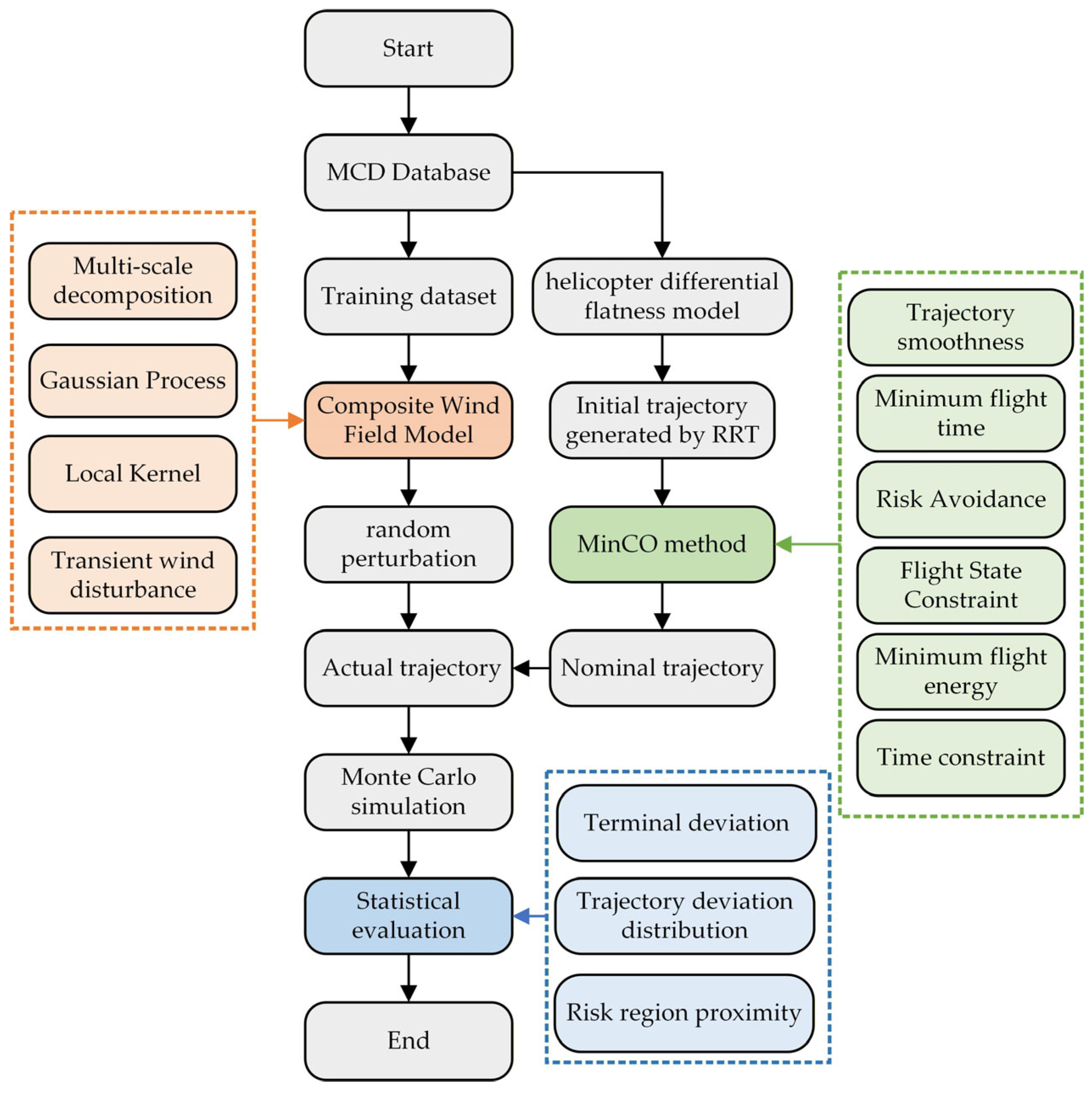
The overall computational framework of the proposed method is illustrated in Figure 3 and consists of the following steps:

(1)

Data extraction and preprocessing: Multiple sets of instantaneous wind field data are extracted from the MCD for the target region and time period to construct a training set for wind disturbance modeling.

(2)

Composite wind field modeling: Based on the training dataset, the multi-scale Gaussian process regression method is employed to train a composite model of wind field disturbances.

(3)

Nominal trajectory generation: Under background mean wind conditions, a nominal trajectory $p_{\mathrm{ref}}(t)$ is generated using the proposed trajectory planning method and serves as the baseline for subsequent robustness evaluation.

(4)

Monte Carlo Simulation:

• Disturbance wind field sampling: A three-dimensional spatially correlated disturbance wind field is generated by sampling from the trained Gaussian process model.
• Trajectory simulation: The sampled disturbance wind field is incorporated into the helicopter dynamic model, and the actual trajectory $p(t)$ under wind disturbances is obtained through numerical simulation based on the nominal trajectory.
• Deviation calculation: Key metrics, including terminal deviation, trajectory deviation distribution, and risk-region crossing frequency, are statistically analyzed based on the simulated trajectories.

(5)

Statistical evaluation: The statistical results are used for robustness evaluation and iterative refinement of trajectory planning parameters.

Figure 3. Trajectory planning framework of the Mars helicopter.

Figure 3. Trajectory planning framework of the Mars helicopter.

4. Simulation and Analysis

Based on the proposed wind field modeling and trajectory planning framework, numerical simulations are conducted under representative Martian environmental conditions. A three-dimensional flight region of $50 \mathrm{m}\times 50 \mathrm{m}\times 10 \mathrm{m}$ is constructed around the landing site of NASA’s Perseverance rover (${18.44}^{\circ }\mathrm{N},{77.45}^{\circ }\mathrm{E}$), covering the operational scale of typical low-altitude maneuvering and hovering tasks for a Mars helicopter. The environmental conditions are set to a solar longitude of local noon, corresponding to a representative period of active near-surface atmospheric dynamics during the Martian daytime. The resulting simulations are used to evaluate trajectory feasibility and robustness in complex wind environments.

4.1. Nominal Trajectory Planning Results

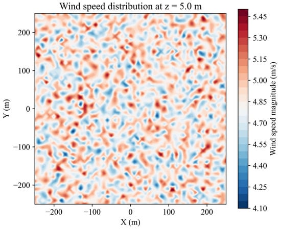
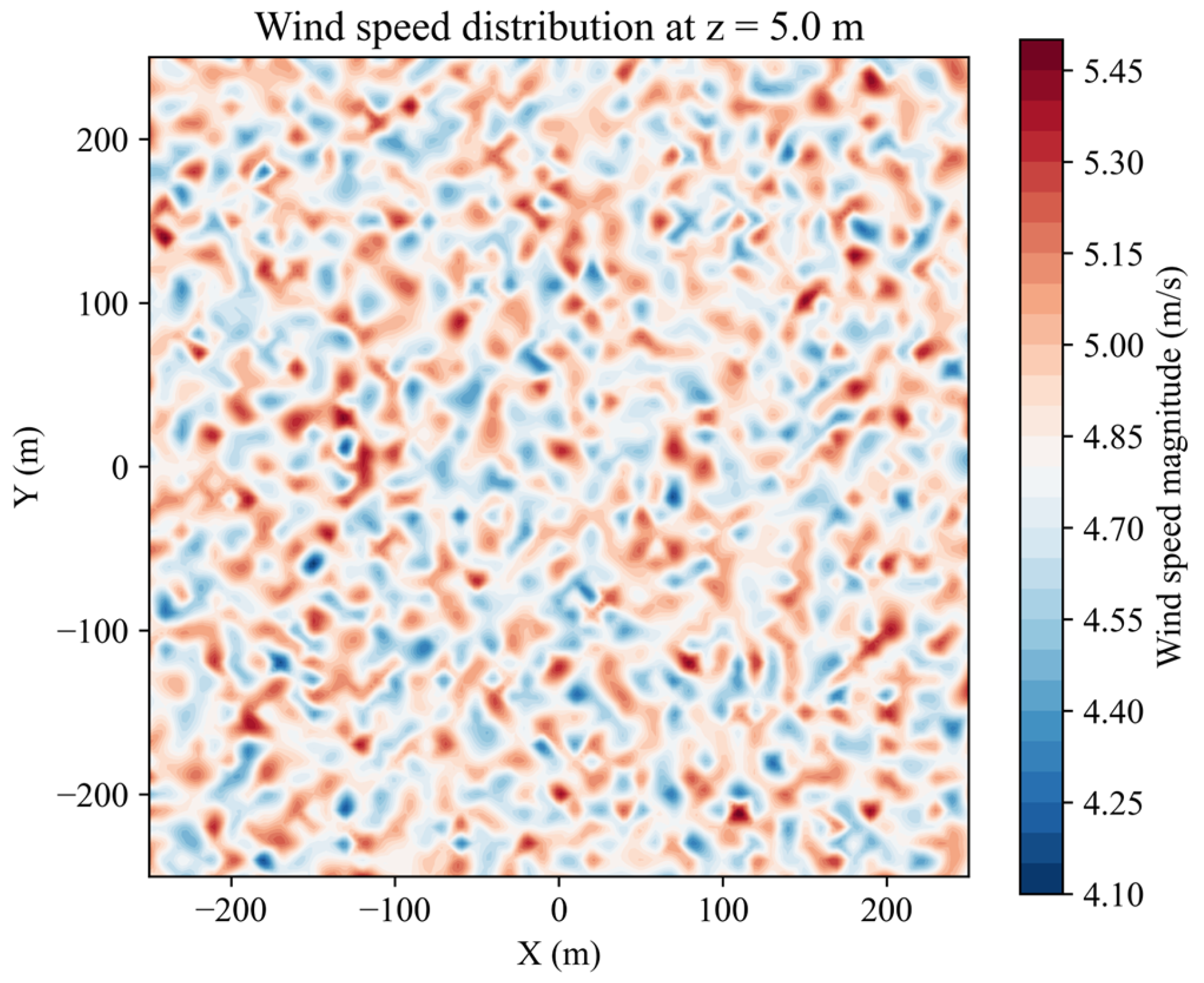
Within the three-dimensional feasible flight region, a representative flight mission is defined by specifying the start and target positions of the Mars helicopter. The start point is set at a near-ground hover state within the region, representing a stable post-takeoff flight condition. The target point is located at another position with significant horizontal displacement while remaining within the allowable low-altitude flight range, corresponding to a typical short-range point-to-point maneuver or local reconnaissance task. Figure 4 shows the wind field distribution at an altitude of 5 m above the surface within the feasible region.

Figure 4. Mean wind field at an altitude of 5 $\mathrm{m}$ above the Martian surface.

The trajectory parameters are configured based on the dynamic characteristics of the Mars helicopter and environmental constraints, with key parameters summarized in Table 1. The weighting coefficients are determined through grid search to balance multiple optimization objectives, including trajectory smoothness, flight time, risk avoidance, state feasibility, and energy consumption.

Table 1. Parameters of the trajectory planner.

Parameters	Value	Unit
$M$	2.2	$\mathrm{kg}$
$v_{th}$	10	$\mathrm{m}/\mathrm{s}$
${\sigma }_{th}$	0.25	$\mathrm{m}/\mathrm{s}$
$\nabla v_{th}$	0.5	---
$T{I}_{th}$	0.1	---
$l_{th}$	1	$\mathrm{m}$
$V_{th}$	10	$\mathrm{m}/\mathrm{s}$

Considering the different physical meanings and numerical scales of the objective terms, the penalty coefficients associated with risk avoidance and state feasibility were first assigned sufficiently large values to ensure effective constraint enforcement. Subsequently, the remaining weighting coefficients for trajectory smoothness, flight time, and energy consumption were tuned iteratively within predefined search ranges until a satisfactory balance among trajectory quality, flight efficiency, and energy consumption was achieved. The search ranges and the final selected weighting coefficients are summarized in Table 2.

Table 2. Search ranges and selected values of the weighting coefficients.

Weight Coefficient	Search Range	Selected Value	Description
${\lambda }_s$	10~30	20	Trajectory smoothness
${\lambda }_t$	20~40	30	Flight time
${\lambda }_r$	1.0 × 103~1.0 × 105	1.0 × 104	Risk avoidance penalty
${\lambda }_f$	1.0 × 103~1.0 × 105	1.0 × 104	State feasibility penalty
${\lambda }_e$	0.1~0.8	0.5	Energy consumption

To validate the generalization capability of the proposed planning method, four sets of start-end point combinations with different spatial locations and wind field environments are selected for simulation validation. As shown in Table 3, the four trajectories differ significantly in start points, end points, path lengths, and along-track wind field characteristics, covering various mission scenarios that a Mars helicopter may encounter.

Table 3. Mission configurations and environmental characteristics of the four trajectories.

Trajectory ID	Start Point ($\mathbf{m}$)	End Point ($\mathbf{m}$)	Trajectory Length ($\mathbf{m}$)	Flight Time ($\mathbf{s}$)	Wind Velocity ($\mathbf{m}/\mathbf{s}$)
1	(−210, −220, 1)	(110, 100, 9)	452.89	48.86	4.859
2	(−200, 200, 1)	(200, −200, 9)	565.88	60.15	4.792
3	(200, 200, 9)	(−200, −200, 9)	566.01	60.14	4.894
4	(−200, 200, 9)	(200, −200, 1)	565.81	60.13	4.827

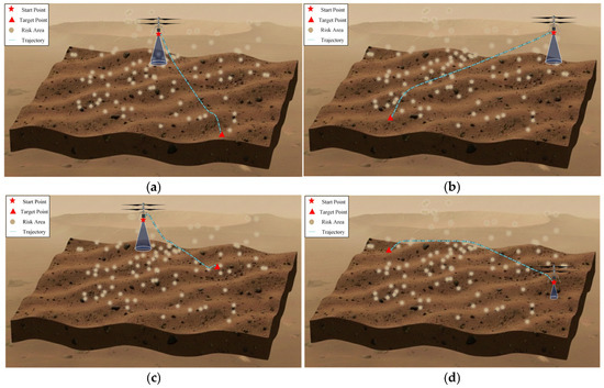
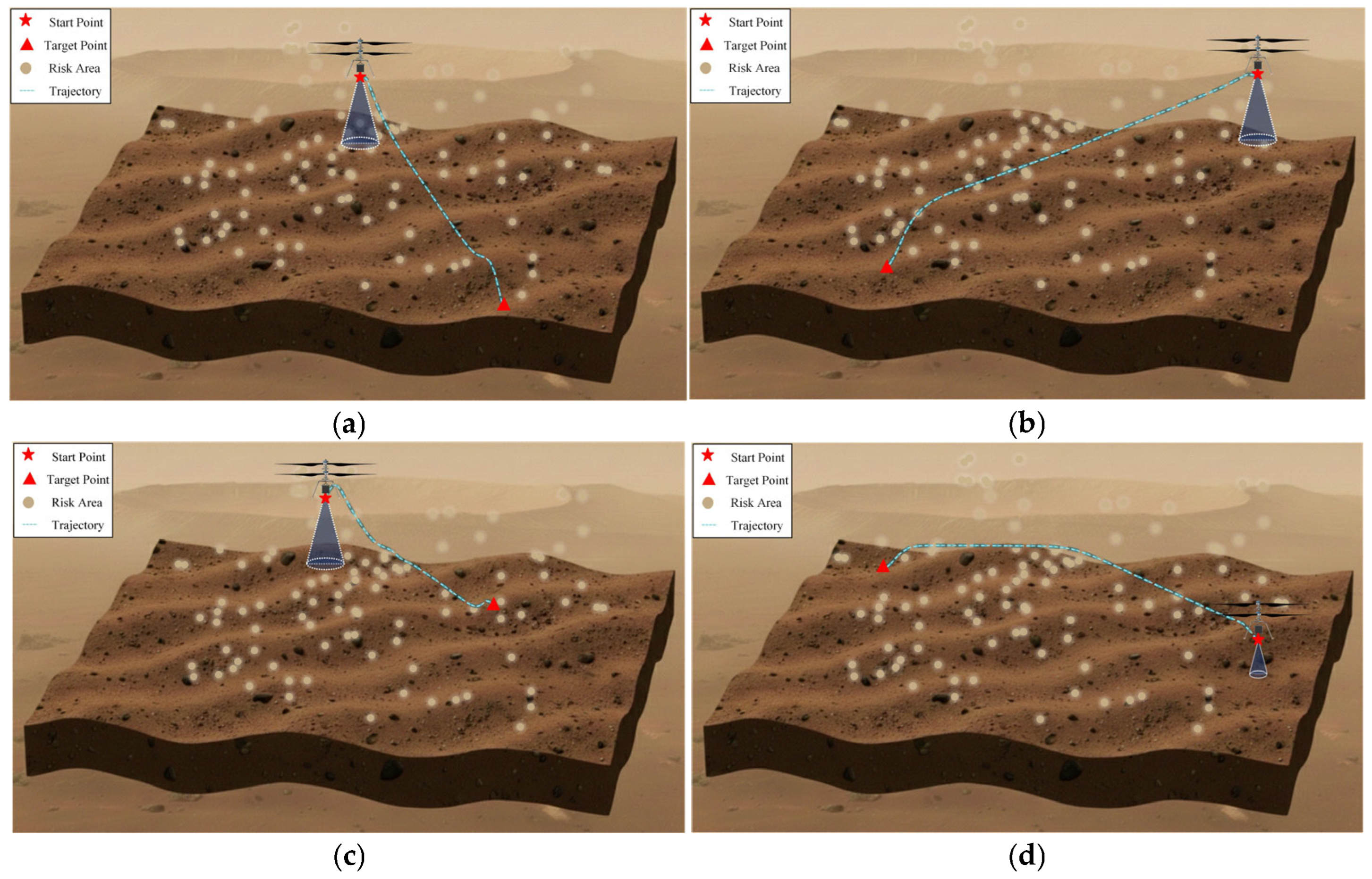
Figure 5 presents the planning results of the four trajectories in three-dimensional space. It can be observed that, under different scenarios, the proposed method consistently generates feasible trajectories that effectively avoid risk regions and successfully reach the target points.

Figure 5. Mars helicopter flight trajectories. (a) Trajectory 1; (b) Trajectory 2; (c) Trajectory 3; (d) Trajectory 4.

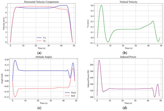
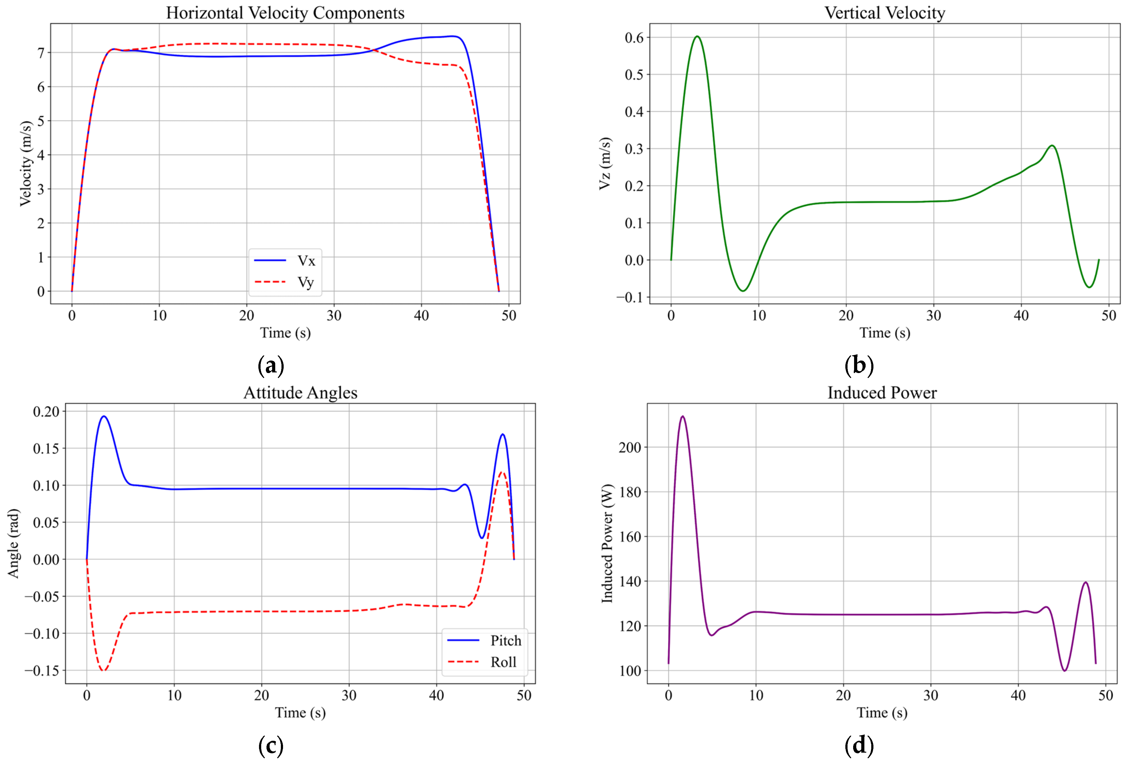
To further analyze flight state evolution under complex wind conditions, Trajectory 1 is selected as a representative case. Figure 6 presents the time histories of key flight parameters for Trajectory 1. The maximum flight speed reaches 10 $\mathrm{m}/\mathrm{s}$, while the maximum attitude angle is 14.07°, both remaining within the allowable flight envelope. In addition, the velocity and attitude profiles are smooth and continuous without abrupt high-frequency variations, indicating stable flight behavior and good continuity of control inputs.

Figure 6. Trajectory 1: Flight parameter profiles of the Mars helicopter. (a) Horizontal velocity profile; (b) Vertical velocity profile; (c) Attitude angles profile; (d) Induced power profile.

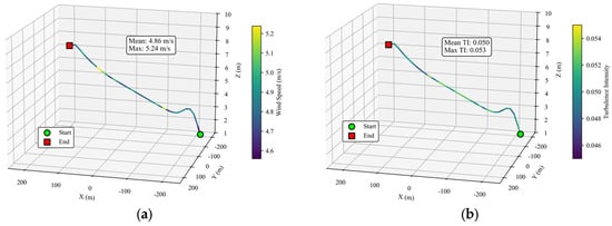
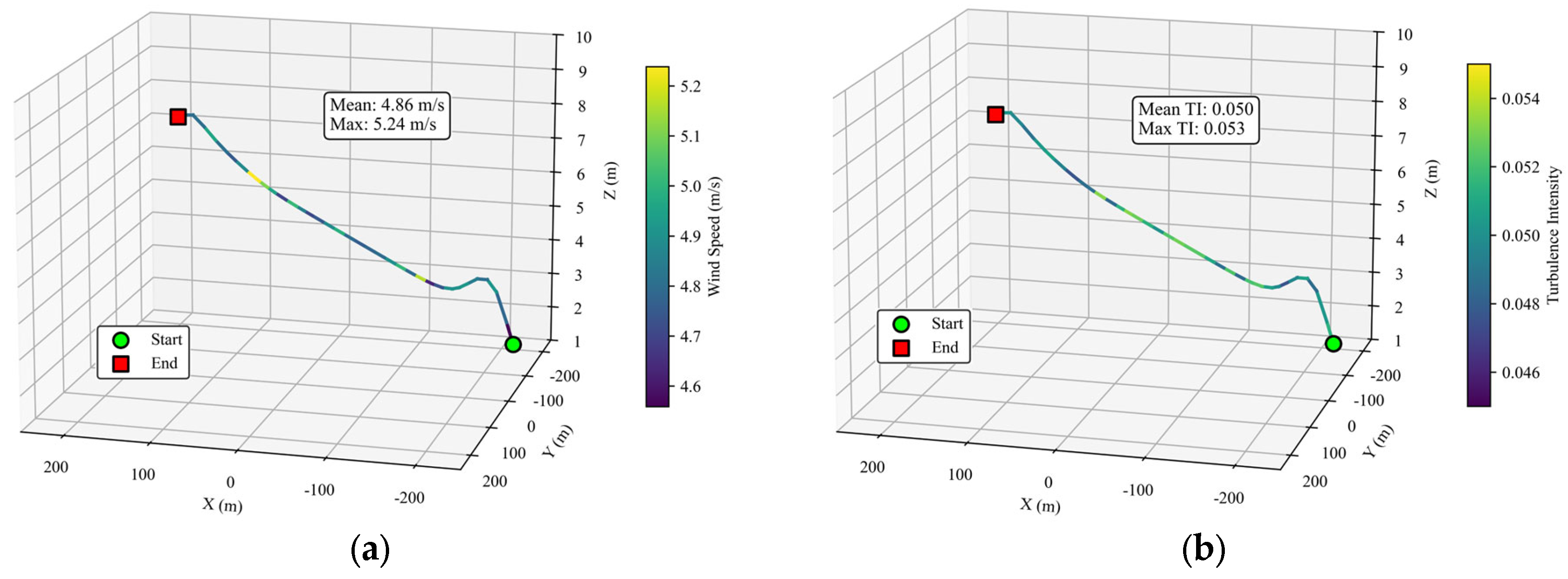
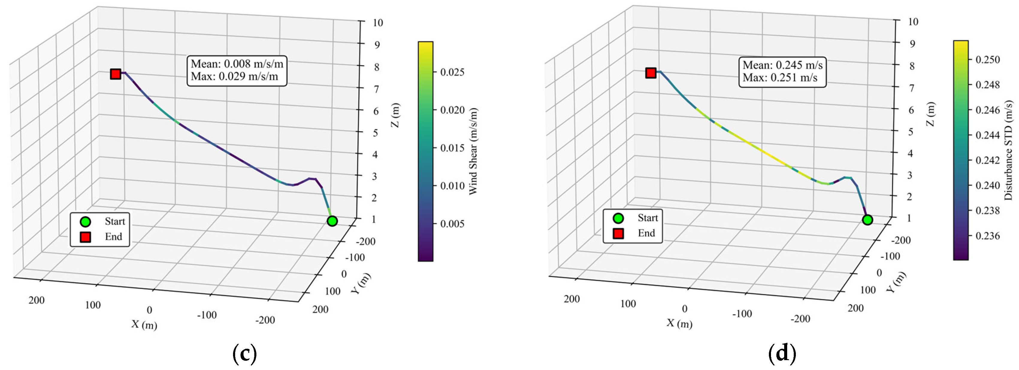
As shown in Figure 7, the wind field characteristics along Trajectory 1 are analyzed based on the risk region criteria. The maximum wind speed along the trajectory is 5.238 $\mathrm{m}/\mathrm{s}$, the maximum wind speed gradient is 0.12 ${\mathrm{s}}^{-1}$, the maximum disturbance standard deviation is 0.251 $\mathrm{m}/\mathrm{s}$, and the maximum turbulence intensity is 0.18. These results indicate that Trajectory 1 effectively avoids the identified risk regions under the proposed statistical criteria.

Figure 7. Along-trajectory variations of wind field characteristics for Trajectory 1. (a) Wind speed distribution; (b) Turbulence intensity distribution; (c) Wind shear distribution; (d) Disturbance standard deviation distribution.

To evaluate the influence of the weighting coefficients on the trajectory planning performance, a sensitivity analysis was conducted by varying the flight-time weighting coefficient ${\lambda }_t$ while keeping the remaining parameters unchanged. The corresponding results are summarized in Table 4.

Table 4. Sensitivity of flight performance to time penalty weight (${\lambda }_t$).

${\mathit{\lambda }}_{\mathit{t}}$	Flight Time ($\mathbf{s}$)	Trajectory Length ($\mathbf{m}$)	Energy ($\mathbf{J}$)	Trajectory Smoothness
20	49.03	455.76	6372.94	54.69
25	48.91	452.85	6369.46	57.05
30	48.86	452.89	6370.94	59.21
35	48.76	449.97	6370.50	61.89
40	49.32	446.62	6373.28	63.04

Note: The penalty terms for risk avoidance and state feasibility are zero in all cases.

As ${\lambda }_t$ increases from 20 to 40, the trajectory length decreases gradually from 455.76 $\mathrm{m}$ to 446.62 $\mathrm{m}$, indicating that a larger flight-time weight encourages the planner to generate more compact trajectories. Meanwhile, the energy consumption remains nearly unchanged, with a maximum variation of less than 0.1%, demonstrating that moderate changes in ${\lambda }_t$ have little influence on the overall energy cost. The trajectory smoothness exhibits a gradual improvement over the tested range, whereas the flight time fluctuates only slightly, with the maximum difference being approximately 0.56 $\mathrm{s}$. These results indicate that the proposed trajectory planner is not overly sensitive to moderate variations in the weighting coefficient, and the selected value (${\lambda }_t$ = 30) provides a balanced trade-off between trajectory efficiency, smoothness, and energy consumption.

4.2. Monte Carlo-Based Evaluation

4.2.1. Simulation Setup

Based on the Gaussian process regression model trained in Section 2.2, 1000 perturbed wind field samples are generated by independently sampling the three-dimensional spatial domain defined by longitude, latitude, and altitude. Dynamic simulations are performed using a nominal controller designed under mean wind conditions to evaluate trajectory robustness under baseline control assumptions. To further investigate trajectory stability under extreme wind conditions, rare strong disturbance cases are introduced into the Monte Carlo simulations shown in Table 5. Specifically, among all samples, a certain proportion is selected to receive additional directional wind perturbations.

Table 5. Disturbance injection settings.

Sample Percentage	Disturbance Condition	Extreme Disturbance
		Magnitude	Direction	Last Time ($\mathbf{s}$)	Injections Count
10%	Base + Extreme	15	Tailwind	5	3
10%	Base + Extreme	15	Random	5	3
10%	Base + Extreme	7	Tailwind	5	3
10%	Base + Extreme	7	Random	5	3
60%	Base	----	----	----	----

These disturbances are applied at random positions along the trajectory and persist for a finite duration to simulate short-term gusts or local strong convection events in the Martian atmosphere. This modeling approach captures both the magnitude characteristics and temporal locality of extreme wind disturbances, ensuring significant disturbance effects while avoiding unphysical accumulation caused by prolonged persistence.

4.2.2. Assessment and Analysis

(1)

Terminal Deviation

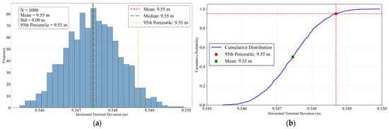
Terminal deviation (TD) is a key metric for evaluating the final positional accuracy of the trajectory under wind field disturbances. The terminal deviation $d_{dev}^{(i)}\left(T\right)$ of the $i^{th}$ simulation, denoted as ${△r}_T$, is defined as:

$$d_{dev}^{(i)}\left(T\right)=‖p^{(i)}(T)-p_{ref}(T)‖$$

(52)

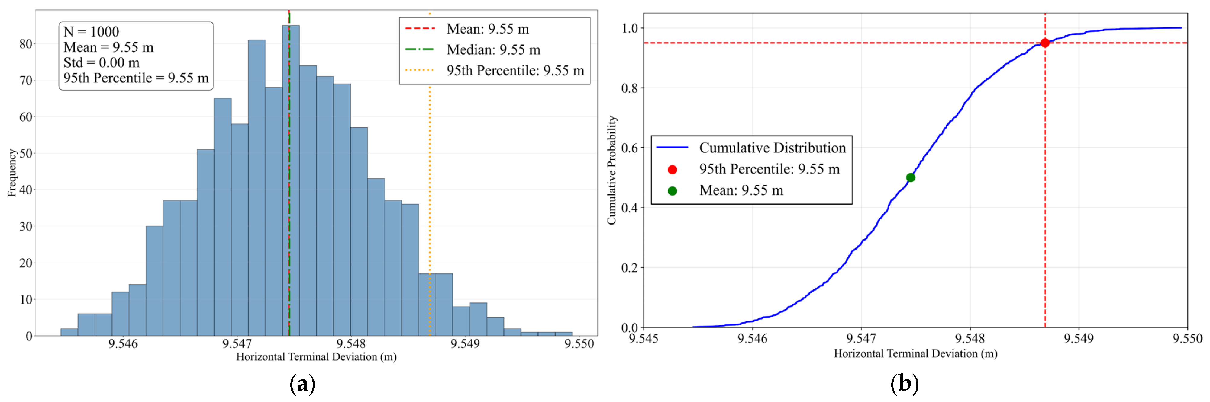
Figure 8 presents the statistical histogram and cumulative distribution function of TD across 1000 simulations. As shown in Figure 8a, the TD follows a unimodal distribution concentrated around 9.55 $\mathrm{m}$, corresponding to approximately 2% of the total trajectory length. This indicates that random wind disturbances do not induce trajectory divergence but instead lead to a statistically stable deviation around the target point. The distribution exhibits limited dispersion without significant long tails or multimodal characteristics, demonstrating good statistical consistency and stability of the trajectory response. However, the concentrated non-zero deviation also indicates limited disturbance compensation capability of the baseline trajectory, resulting in a residual systematic error that may require further correction through trajectory refinement or control optimization.

Figure 8. Statistical distribution of TD. (a) TD histogram; (b) TD cumulative distribution function.

The cumulative distribution function shown in Figure 8b further quantifies the probabilistic bound of TD. The results indicate that the 95th percentile of terminal deviation is approximately 9.55 $\mathrm{m}$, meaning that 95% of simulated trajectories remain within this error range. This demonstrates that the TD remains statistically bounded under random wind disturbances. Since no explicit disturbance rejection strategy is introduced in this study, the concentrated non-zero deviation primarily reflects the direct influence of wind field uncertainty on trajectory performance.

(2)

Risk Region Proximity

Risk region proximity is used as a safety metric to quantify the relative position of the trajectory with respect to high-risk areas. Based on the comprehensive risk region criteria, the corresponding risk region distribution is constructed within the flight domain using multiple indicators, including maximum wind speed, wind velocity gradient, disturbance standard deviation, and turbulence intensity.

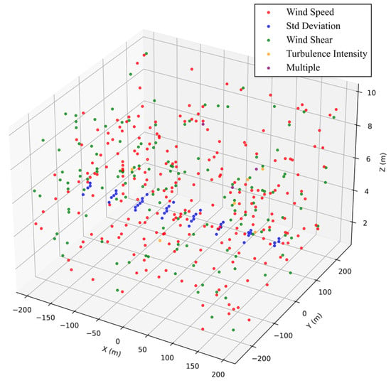
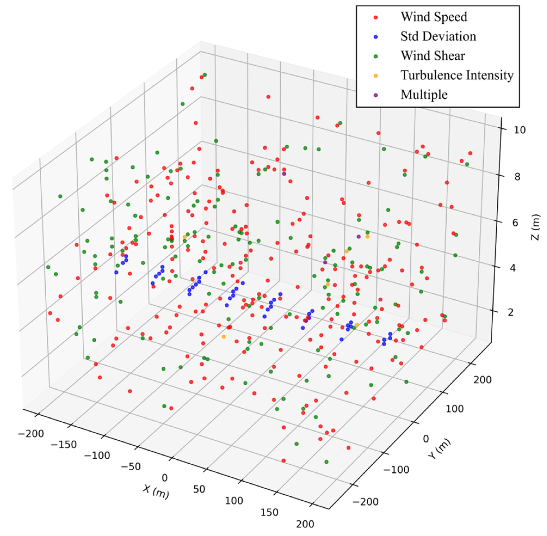
Figure 9 presents the spatial distribution of identified risk regions, with different colors indicating different risk trigger types. Statistical results show that a total of 431 potential risk regions are detected, among which 237 are triggered by the maximum wind speed threshold, 143 by wind velocity gradient, 42 by the disturbance standard deviation threshold, and 6 by turbulence intensity. In addition, three regions are simultaneously triggered by multiple risk factors. These risk regions are spatially scattered and primarily concentrated in localized areas with large wind speed disturbances or significant wind velocity gradients.

Figure 9. Spatial distribution of risk regions.

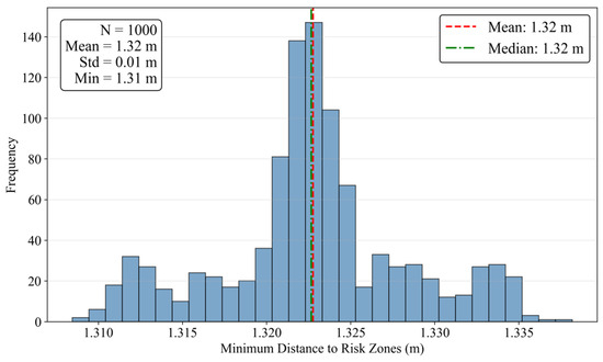
To quantitatively evaluate the safety of the nominal trajectory under stochastic wind disturbances, the minimum distance $d_{\min }^{(i)}$ between the trajectory and the risk regions is computed for the $i^{th}$ simulation and defined as:

$$d_{\min }^{(i)}=\underset{p_r\in \mathcal{A}}{\min }\underset{t\in \left[0,T\right]}{\min }‖p^{(i)}(t)-p_r‖$$

(53)

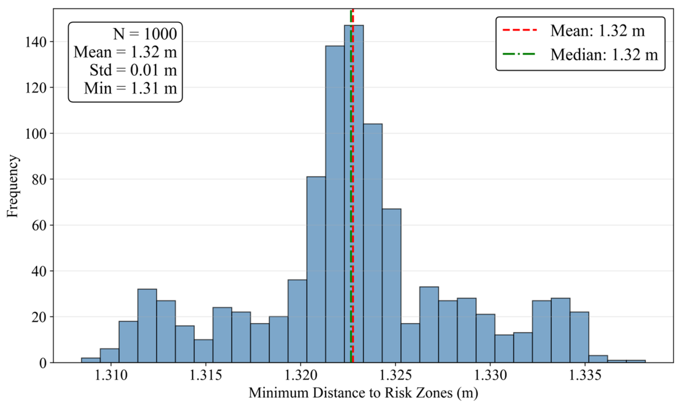
Figure 10 presents the statistical histogram of the minimum distance between the trajectory and identified risk regions in the Monte Carlo simulations. All samples remain above the preset safety threshold, indicating that the nominal trajectory does not enter any risk region under random wind disturbances, corresponding to a zero risk-region crossing probability. The mean minimum distance is 1.32 $\mathrm{m}$ with a standard deviation of 1.32 $\mathrm{m}$, indicating a certain degree of variability in safety margin under different disturbance conditions while maintaining overall risk avoidance performance.

Figure 10. Histogram of risk region proximity.

These results demonstrate that the proposed risk avoidance constraints remain effective under stochastic wind disturbances, providing probabilistic support for safe Mars helicopter flight in complex wind environments.

(3)

Trajectory Dispersion

Trajectory dispersion is used to quantify the deviation of the trajectory under wind disturbances, reflecting its consistency and stability in uncertain environments. In this study, two metrics are adopted: the maximum deviation distance, which characterizes the largest deviation during flight, and the average dispersion distance, which measures the overall deviation level. The instantaneous deviation distance $d_{dev}^{(i)}\left(t\right)$ between the simulated trajectory and the nominal trajectory at time $t$ in the $i^{th}$ simulation is defined as:

$$d_{dev}^{(i)}\left(t\right)=‖p^{(i)}(t)-p_{ref}(t)‖$$

(54)

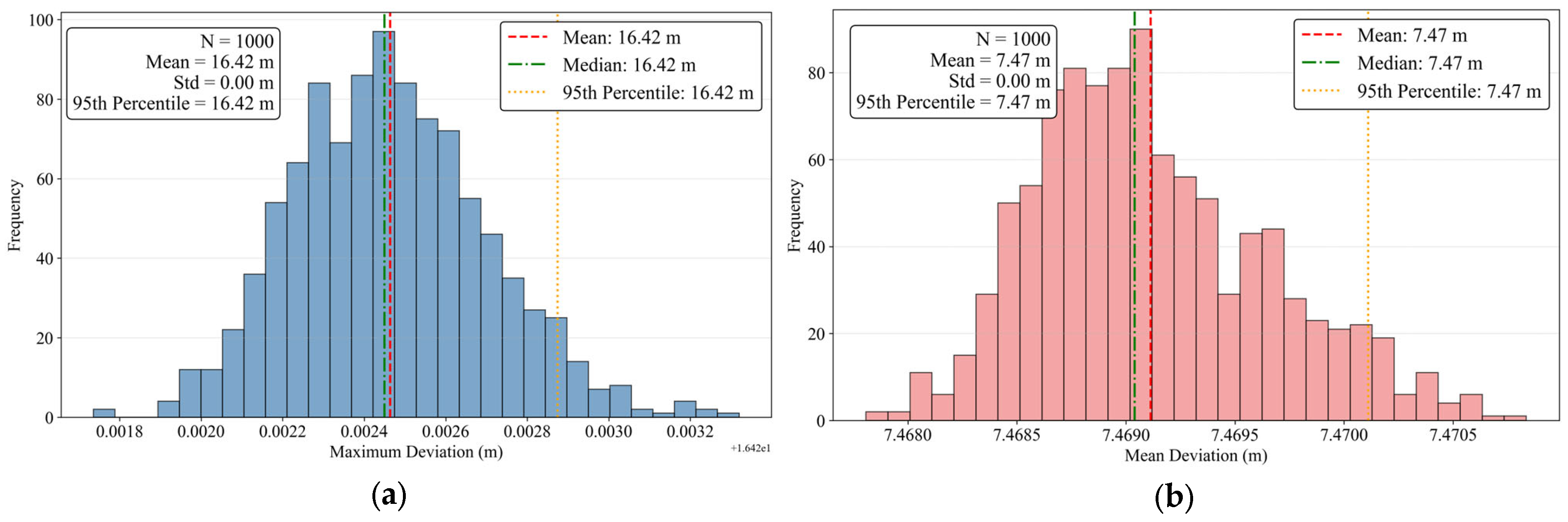
Figure 11a presents the statistical histogram of the maximum deviation distance in the Monte Carlo simulations. The mean maximum deviation distance is 16.42 $\mathrm{m}$, corresponding to approximately 3.6% of the total trajectory length. The distribution is concentrated within a finite range without obvious long tails or divergent behavior, indicating that the extreme trajectory deviation remains statistically bounded under random wind disturbances. This suggests that the rotorcraft generally maintains a limited deviation from the baseline trajectory in most simulation cases.

Figure 11. Statistical distribution of trajectory deviation. (a) Histogram of maximum deviation distance; (b) Histogram of mean dispersion.

Figure 11b presents the statistical histogram of the mean deviation distance. Compared with the maximum deviation distance, the mean deviation remains at a relatively low level, with an average value of 7.47 $\mathrm{m}$, corresponding to approximately 1.6% of the total trajectory length. This indicates that trajectory deviations remain limited during most of the flight. The relatively small mean deviation compared with the maximum deviation further suggests that large deviations mainly occur in localized time intervals rather than accumulating continuously throughout the flight.

These results indicate that both extreme and average trajectory deviations remain statistically bounded under random wind disturbances, supporting the stability of the baseline trajectory in uncertain environments.

(4)

Multi-Trajectory Evaluation

To further evaluate the generalization capability and robustness of the proposed trajectory planning method, Monte Carlo simulations are conducted for each of the four trajectories described in Section 4.1. Key metrics, including terminal deviation, maximum trajectory deviation, mean deviation, and risk-region crossing probability, are statistically analyzed. The robustness assessment results for all four trajectories are summarized in Table 6.

Table 6. Statistical distribution of multiple trajectories.

Trajectory ID	TD ($\mathbf{m}$)	Max Deviation ($\mathbf{m}$)	Mean Deviation ($\mathbf{m}$)	Risk Region Crossing
1	9.55 (2.1%)	16.42 (3.6%)	7.47 (1.6%)	0
2	9.98 (1.8%)	16.49 (2.9%)	6.93 (1.2%)	0
3	9.53 (1.7%)	15.19 (2.7%)	6.82 (1.2%)	0
4	10.64 (1.9%)	17.63 (3.1%)	7.53 (1.3%)	0

Where the percentages in parentheses denote the ratio of the current deviation distance to the total trajectory length.

Across all four trajectories, the robustness metrics exhibit similar statistical characteristics. The mean terminal deviation ranges from approximately 9.5 $\mathrm{m}$ to 10.6 $\mathrm{m}$ (1.7–2.1% of trajectory length), while the maximum deviation distance remains within 15–18 m (2.7–3.6%), indicating bounded trajectory responses under wind disturbances. The mean deviation distance is consistently maintained within 6.8–7.5 m (1.2–1.6%), suggesting limited overall deviation throughout the flight. In addition, none of the trajectories enter identified risk regions in any Monte Carlo simulation, resulting in zero risk-region crossing probability for all cases and confirming the effectiveness of the proposed safety constraints.

In summary, the four trajectories with different start and target configurations yield consistent robustness metrics, demonstrating that the proposed method performs reliably across a range of representative mission configurations.

5. Conclusions

This paper addresses the challenge of uncertain wind disturbances encountered by Mars helicopters operating in low-density atmospheric environments. A trajectory planning and robustness evaluation framework based on composite wind field modeling, differential flatness, and Monte Carlo simulation is proposed under a decoupled paradigm of deterministic planning and statistical evaluation. Numerical results demonstrate that the proposed method can generate dynamically feasible and risk-aware trajectories under complex wind conditions while maintaining bounded statistical deviations and zero risk-region crossing probability in Monte Carlo simulations. These results verify the effectiveness and robustness of the proposed planning framework and provide a practical solution for autonomous Mars helicopter missions under limited onboard computational resources. The main conclusions are summarized as follows:

(1)

By combining multi-scale decomposition with Gaussian process regression, a composite wind field model is established to capture both spatial correlation and transient disturbance characteristics. The introduced local kernel technique effectively balances modeling accuracy and computational efficiency, enabling probabilistic characterization of Martian wind field uncertainty for subsequent trajectory planning and robustness evaluation.

(2)

The differential flatness- and MinCo-based trajectory planning method generates high-order polynomial trajectories with favorable dynamic continuity and physical feasibility. By incorporating a multi-dimensional optimization objective including energy consumption, flight time, trajectory smoothness, risk avoidance, and flight state feasibility, the planned trajectories effectively avoid risk regions defined by wind speed, wind velocity gradient, disturbance intensity, and turbulence characteristics.

(3)

Monte Carlo simulation results demonstrate the effectiveness and robustness of the proposed method in complex wind environments. Across the four representative trajectory scenarios, the risk-region crossing probability is zero for all cases, while the mean terminal deviation, mean deviation, and maximum deviation distance remain within 2.1%, 1.6%, and 3.6% of the corresponding trajectory lengths, respectively. These results confirm that the proposed method maintains bounded trajectory deviations while consistently satisfying safety constraints under stochastic wind disturbances, demonstrating good statistical robustness for the scenarios considered in this study.

In the future, the risk region identification could be refined using probabilistic or data-driven methods, the robustness evaluation could be extended to incorporate control-level uncertainties such as actuator dynamics and model mismatches, and further validation could be conducted under a broader range of scenarios.

References

- Withrow, S.; Johnson, W.; Young, L.A.; Koning, W. Mars science helicopter conceptual design. In Proceedings of the ASCEND 2020, Online, 16–18 November 2020; p. 4029. [Google Scholar]
- Balaram, B.; Canham, T.; Duncan, C.; Grip, H.F.; Johnson, W.; Maki, J.; Quon, A.; Stern, R.; Zhu, D. Mars helicopter technology demonstrator. In Proceedings of the 2018 AIAA Atmospheric Flight Mechanics Conference, Kissimmee, FL, USA, 8–12 January 2018; p. 0023. [Google Scholar]
- Grip, H.F.; Scharf, D.P.; Malpica, C.; Johnson, W.; Mandic, M.; Singh, G.; Young, L.A. Guidance and control for a Mars helicopter. In Proceedings of the 2018 AIAA Guidance, Navigation, and Control Conference, Kissimmee, FL, USA, 8–12 January 2018; p. 1849. [Google Scholar]
- Balaram, J.; Aung, M.M.; Golombek, M.P. The ingenuity helicopter on the perseverance rover. Space Sci. Rev. 2021, 217, 56. [Google Scholar] [CrossRef] [Scilit]
- Tzanetos, T.; Aung, M.M.; Balaram, J.; Grip, H.F.; Karras, J.T.; Canham, T.K.; Kubiak, G.; Anderson, J.; Merewether, G.; Starch, M.; et al. Ingenuity mars helicopter: From technology demonstration to extraterrestrial scout. In Proceedings of the 2022 IEEE Aerospace Conference (AERO); IEEE: New York, NY, USA, 2022; pp. 1–19. [Google Scholar]
- Rafkin, S.; Michaels, T. The Mars regional atmospheric modeling system (MRAMS): Current status and future directions. Atmosphere 2019, 10, 747. [Google Scholar] [CrossRef] [Scilit]
- Justh, H.L.; Burns, K.L.; Dutta, S.; Hoffman, J. Mars Global Reference Atmospheric Model (Mars-GRAM) 2024: User Guide; National Aeronautics and Space Administration: Washington, DC, USA, 2024. [Google Scholar]
- Ågren, T.S.; Ruan, A.W.; Malpica, C.; Withrow-Maser, S. In-flight System Identification of the Ingenuity Mars Helicopter. J. Guid. Control Dyn. 2026, 49, 1005–1022. [Google Scholar] [CrossRef] [Scilit]
- Millour, E.; Forget, F.; Spiga, A.; Vals, M.; Zakharov, V.; Montabone, L.; Lefèvre, F.; Montmessin, F.; Chaufray, J.-Y.; López-Valverde, M.A.; et al. The Mars climate database (version 5.3). In Proceedings of the Scientific Workshop: “From Mars Express to ExoMars”, Madrid, Spain, 27–28 February 2018; p. 68. [Google Scholar]
- Bingham, S.J.; Lewis, S.R.; Read, P.L.; Forget, F.; Hourdin, F.; Talagrand, O.; Wanherdrick, Y.; Angelats i Coll, M.; Lopez-Valverde, M.; Lopez-Puertas, M.; et al. The Mars Climate Database. In Proceedings of the First International Workshop on Mars Atmosphere Modelling and Observations, Granada, Spain, 13–15 January 2003. [Google Scholar]
- Piccione, G. Modeling and Control of a Space Drone for Mars Exploration Mission. Master’s Thesis, Politecnico di Torino, Torino, Italy, 2021. [Google Scholar]
- Jackson, B.; Fenton, L.; Brown, T.; Munguira, A.; Martinez, G.; Newman, C.; Viúdez-Moreiras, D.; Golombek, M.; Lorenz, R.; Paton, M.D.; et al. Profiling Near-surface Winds on Mars Using Attitude Data from Mars 2020 Ingenuity. Planet. Sci. J. 2025, 6, 21. [Google Scholar] [CrossRef] [Scilit]
- Hong, Z.; Zhiwei, D.; Gen, L.; Li, J. Flight dynamics modeling and analysis for a Mars helicopter. Chin. J. Aeronaut. 2023, 36, 221–230. [Google Scholar] [CrossRef] [Scilit]
- Nasir, J.; Islam, F.; Malik, U.; Ayaz, Y.; Hasan, O.; Khan, M.; Muhammad, M.S. RRT*-SMART: A rapid convergence implementation of RRT. Int. J. Adv. Robot. Syst. 2013, 10, 299. [Google Scholar] [CrossRef] [Scilit]
- Karaman, S.; Frazzoli, E. Sampling-based algorithms for optimal motion planning. Int. J. Robot. Res. 2011, 30, 846–894. [Google Scholar] [CrossRef] [Scilit]
- Paden, B.; Čáp, M.; Yong, S.Z.; Yershov, D.; Frazzoli, E. A survey of motion planning and control techniques for self-driving urban vehicles. IEEE Trans. Intell. Veh. 2016, 1, 33–55. [Google Scholar] [CrossRef] [Scilit]
- Rawlings, J.B.; Mayne, D.Q.; Diehl, M.M. Model Predictive Control: Theory, Computation, and Design; Nob Hill Publishing, LLC: Madison, WI, USA, 2020. [Google Scholar]
- Fliess, M.; Lévine, J.; Martin, P.; Rouchon, P. Flatness and defect of non-linear systems: Introductory theory and examples. Int. J. Control 1995, 61, 1327–1361. [Google Scholar] [CrossRef] [Scilit]
- Fliess, M.; Lévine, J.; Martin, P.; Rouchon, P. A lie-backlund approach to equivalence and flatness of nonlinear systems. IEEE Trans. Autom. Control 2002, 44, 922–937. [Google Scholar]
- Duan, D.; Zu, R.; Yu, T.; Zhang, C.; Li, J. Differential flatness-based real-time trajectory planning for multihelicopter cooperative transportation in crowded environments. AIAA J. 2023, 61, 4079–4095. [Google Scholar] [CrossRef] [Scilit]
- Mesbah, A. Stochastic model predictive control: An overview and perspectives for future research. IEEE Control Syst. Mag. 2016, 36, 30–44. [Google Scholar] [CrossRef] [Scilit]
- Blackmore, L.; Ono, M.; Williams, B.C. Chance-constrained optimal path planning with obstacles. IEEE Trans. Robot. 2011, 27, 1080–1094. [Google Scholar] [CrossRef] [Scilit]
- Patel, A. Design, Modelling and Control of a Space UAV for Mars Exploration. Master’s Thesis, Luleå University of Technology, Luleå, Sweden, 2021. [Google Scholar]
- Mellinger, D.; Kumar, V. Minimum snap trajectory generation and control for quadrotors. In Proceedings of the 2011 IEEE International Conference on Robotics and Automation; IEEE: New York, NY, USA, 2011; pp. 2520–2525. [Google Scholar]
- Viadero-Monasterio, F.; Meléndez-Useros, M.; Zhang, N.; Zhang, H.; Boada, B.L.; Boada, M.J.L. Motion planning and robust output-feedback trajectory tracking control for multiple intelligent and connected vehicles in unsignalized intersections. IEEE Trans. Veh. Technol. 2025, 74, 18543–18555. [Google Scholar] [CrossRef] [Scilit]
- Williams, C.K.I.; Rasmussen, C.E. Gaussian Processes for Machine Learning; MIT Press: Cambridge, MA, USA, 2006. [Google Scholar]
- Nguyen-Tuong, D.; Seeger, M.; Peters, J. Model learning with local gaussian process regression. Adv. Robot. 2009, 23, 2015–2034. [Google Scholar] [CrossRef] [Scilit]
- Wang, Z.; Zhou, X.; Xu, C.; Gao, F. Geometrically constrained trajectory optimization for multicopters. IEEE Trans. Robot. 2022, 38, 3259–3278. [Google Scholar] [CrossRef] [Scilit]
- Bangura, M.; Mahony, R. Nonlinear dynamic modeling for high performance control of a quadrotor. In Proceedings of the Australasian Conference on Robotics and Automation, Wellington, New Zealand, 3–5 December 2012. [Google Scholar]
- Faessler, M.; Franchi, A.; Scaramuzza, D. Differential flatness of quadrotor dynamics subject to rotor drag for accurate tracking of high-speed trajectories. IEEE Robot. Autom. Lett. 2017, 3, 620–626. [Google Scholar] [CrossRef] [Scilit]
- Tal, E.; Karaman, S. Accurate tracking of aggressive quadrotor trajectories using incremental nonlinear dynamic inversion and differential flatness. IEEE Trans. Control Syst. Technol. 2020, 29, 1203–1218. [Google Scholar] [CrossRef] [Scilit]
- Johnson, W. Helicopter Theory; Courier Corporation: North Chelmsford, MA, USA, 2012. [Google Scholar]
- James, F. Monte Carlo theory and practice. Rep. Prog. Phys. 1980, 43, 1145–1189. [Google Scholar] [CrossRef] [Scilit]
- O’dwyer, A. Handbook of PI and PID Controller Tuning Rules; World Scientific: Singapore, 2009. [Google Scholar]
Disclaimer/Publisher’s Note: The statements, opinions and data contained in all publications are solely those of the individual author(s) and contributor(s) and not of MDPI and/or the editor(s). MDPI and/or the editor(s) disclaim responsibility for any injury to people or property resulting from any ideas, methods, instructions or products referred to in the content. |
© 2026 by the authors. Licensee MDPI, Basel, Switzerland. This article is an open access article distributed under the terms and conditions of the Creative Commons Attribution (CC BY) license.