


Abstract
The widespread application of drones in complex environments imposes higher demands on flight safety. However, traditional anomaly detection methods often rely on mathematical models or large amounts of labeled samples, which makes them ill suited to address practical challenges such as unmanned aerial vehicle systems, which exhibit strong nonlinear characteristics, a scarcity of fault samples, and highly variable operating conditions. To overcome the above difficulties, this work puts forward a one-dimensional selective kernel convolutional autoencoder (1-D SKCAE) based on Bayesian optimization for unsupervised drone anomaly detection. Relying solely on normal operation data, this model achieves accurate anomaly identification by leveraging the sudden changes in reconstruction error. For the model architecture, this paper designs a multi-scale selective kernel convolution module and combines an attention mechanism to achieve adaptive feature weighting for various receptive fields. This method effectively improves the model’s ability to represent complex operational conditions and subtle fault characteristics. Simultaneously, Bayesian optimization is embedded into the model training process as a hyperparameter search strategy, enabling the adaptive configuration of key hyperparameters to further enhance detection performance. Extensive experiments were conducted using the RflyMAD simulation dataset and the 3DR Solo real flight dataset. The results demonstrate that the 1-D SKCAE outperforms multiple comparative models, exhibiting superior robustness particularly in complex scenarios such as mixed multi-fault superposition. This method enables drone anomaly detection without fault labels, showcasing strong potential for engineering applications.
1. Introduction
As the core vehicle of the low-altitude economy, drones play an irreplaceable role in driving the transformation of emerging industries worldwide and establishing a three-dimensional economic development pattern [1]. Compared with traditional manual operations and conventional transportation, drones offer significant advantages, including high operational efficiency, strong environmental adaptability, low overall costs, and the ability to overcome spatial constraints in complex scenarios [2]. Amid expanding policy dividends for the low-altitude economy and rising demands for intelligent upgrades across industries, drones have become a key driver in activating new productive forces and advancing industrial restructuring [3].
However, when drones undertake highly challenging and hazardous missions, their components may sustain varying degrees of damage, which significantly impacts flight safety [4]. During operations, drones frequently encounter complex working environments such as severe weather, strong winds, extended flight durations, and overloaded payloads, all of which substantially increase the probability of malfunctions. Whether performing high-precision surveying, real-time monitoring, military reconnaissance, or emergency rescue missions, flight safety remains the paramount concern for drones [5,6]. Particularly during flight, failures in critical components like propellers, batteries, power systems, sensors, or communication modules can cause uncontrolled flight or crashes, posing severe threats to personnel and equipment [7,8]. Therefore, researching anomaly detection technologies for drones is crucial for the timely identification of potential failure risks and ensuring flight safety.
Traditional drone anomaly detection methods primarily include model-based and knowledge-based approaches [9,10]. Model-based approaches rely on physical laws or system identification techniques to construct mathematical models of the system, featuring advantages such as excellent real-time capability and superior interpretability [11]. However, given that they have a typical multi-sensor closed-loop flight control system, drones exhibit complex characteristics, including multivariability, time-varying behavior, strong coupling, and high nonlinearity. This poses significant challenges to the construction of robust, high-precision mathematical diagnostic models [12]. Knowledge-based methods, by contrast, do not rely on precise system models but instead detect anomalies through expert experience or historical operational data [13]. However, such approaches typically depend heavily on prior knowledge and large amounts of high-quality historical data, which results in relatively limited generalization capabilities and adaptability to changing operating conditions.
In recent years, along with the rapid progress of sensor and data acquisition technologies, data-driven anomaly detection methods have gradually emerged as a research hotspot [14,15]. Due to the high complexity of drone systems, traditional approaches based on physical models or empirical rules struggle to adapt effectively. Data-driven methods, by automatically mining latent fault features from historical operational data, have become a crucial solution to this challenge [16,17]. The core advantage of data-driven methods lies in their independence from precise physical models or excessive assumptions. Instead, they analyze drones’ operational data to automatically extract fault features, enabling more flexible and adaptable anomaly detection. Based on different learning approaches, data-driven anomaly detection approaches can be mainly divided into supervised learning and unsupervised learning [18,19]. Supervised learning identifies different types of anomalies by learning the distribution features and patterns of labeled data. Li et al. [20] proposed a framework called Siamese Hybrid Neural Network, which achieves intelligent anomaly detection for fixed-wing drones through a few-shot learning strategy. By introducing a “state mapping” strategy, this framework converts flight data into pairs of similar or dissimilar data points, enabling effective fault classification and diagnosis even with limited data. Kim et al. [21] constructed a data-driven model using inertial sensor data and supervised learning methods to detect thrust anomalies in multirotor drones. Thanaraj et al. [22] employed a neural fuzzy system based on extreme learning to achieve anomaly detection and isolation in multirotor drone actuators. Al-Haddad et al. [23] conducted anomaly detection research on drone actuator damage by combining embedded recorded data with stacked machine learning models. Park et al. [24] introduced an unsupervised learning-based anomaly detection method for drones. By extracting key features from flight logs and constructing a stacked autoencoder model to characterize normal flight states, they enhanced the generalization capability of anomaly detection, without requiring extensive labeled data. Zhou et al. [25] achieved efficient anomaly detection and localization in unbalanced drone flight data by suppressing noise through wavelet analysis and modeling normal flight patterns using unsupervised autoencoders. Yang et al. [26] put forward an unsupervised anomaly detection method for drone flight data based on spatio-temporal correlation and LSTMAE. Through filtering preprocessing and correlation-driven feature extraction, this approach enables effective identification of flight anomalies and data recovery in complex noisy environments. Wang et al. [27] developed a method relying on deep ensemble autoencoders, integrating Savitzky–Golay filtering, 1-D convolutional neural networks, and autoencoders to achieve anomaly detection and key parameter identification for drone actuators. Jiang et al. [28] constructed an unsupervised anomaly detection framework for drones based on spatio-temporal autoencoders. By utilizing a multilayer network architecture to acquire spatio-temporal features from flight data and incorporating robust loss functions, they enhanced the model’s adaptability to noise interference. Jasra et al. [29] systematically compared multiple deep learning models within an autoencoder framework for flight data anomaly detection. Their results indicate that LSTM with integrated self-attention mechanisms demonstrates superior detection performance and generalization capabilities. Wang et al. [30] achieved unsupervised anomaly detection in drones’ flight data through self-supervised contrastive learning and graph attention-based spatio-temporal modeling, enhancing fault identification interpretability via reconstruction error analysis. Jasra et al. [31] combined the Local Outlier Factor with statistical thresholding methods to achieve efficient detection of anomalous behaviors in real flight data, effectively reducing the false alarms inherent in traditional unsupervised approaches.
Although the aforementioned methods demonstrate effective anomaly detection capabilities for drones, their widespread adoption still faces several critical challenges. First, supervised learning methods heavily rely on large volumes of precisely labeled anomaly samples. However, acquiring high-quality labeled data in real-world drone operating environments is extremely difficult: on the one hand, actual failure events are low frequency and high risk, making active reproduction challenging; on the other hand, failure modes are diverse with blurred boundaries, leading to costly manual annotation that is prone to introducing subjective bias. This data bottleneck causes supervised models to exhibit significantly degraded generalization performance when encountering unseen anomaly types. Secondly, existing convolutional autoencoder models typically employ fixed-size convolutional kernels for feature extraction, with their receptive fields remaining static during forward propagation. This rigid design cannot adaptively adjust the size of the receptive field based on the local context of the input signal, thereby limiting the network’s ability to dynamically perceive and effectively aggregate multi-scale information. Simultaneously, model performance exhibits high sensitivity to hyperparameter configurations, yet current tuning processes primarily rely on manual trial-and-error or coarse-grained grid searches. The combination space for key hyperparameters—such as the structural depth of the autoencoder, hidden layer dimension, convolutional kernel size, and learning rate—is vast. Traditional parameter tuning strategies not only incur high computational costs and suffer from low efficiency but also struggle to guarantee global optimality. In the absence of unified prior knowledge, this empirically driven optimization approach severely undermines the model’s transferability across different drone platforms and mission scenarios.
Nevertheless, existing studies on UAV anomaly detection mostly address only one of the above limitations in isolation. Few works have systematically integrated adaptive multi-scale feature extraction, an unsupervised autoencoder architecture, and automated hyperparameter optimization into a unified framework tailored to the temporal characteristics of UAV flight data. Conventional unsupervised autoencoder-based methods are either restricted to fixed convolutional kernels and lack dynamic perception of multi-scale fault patterns or rely on empirical hyperparameter tuning that fails to ensure stable performance across diverse UAV platforms and operating conditions. This research gap motivates the present work to construct a targeted detection framework through the organic combination of multiple technical components rather than a simple assembly of existing algorithms.
There have been abundant research achievements in the field of UAV anomaly detection. To intuitively clarify the technical hierarchy and research scope of existing methods, this paper sorts out relevant literature according to the evolution stages of algorithms, as shown in Table 1. It can be found that most existing autoencoder models lack the capability of adaptive time-series feature extraction, and few studies integrate Bayesian optimization for intelligent hyperparameter tuning. To fill this research gap, this paper constructs a 1-D SKCAE unsupervised anomaly detection model, with the core research objectives of adaptive feature extraction and automatic hyperparameter optimization, which distinctly highlights the innovation value of this work.
Table 1.
Summary of Existing Research on UAV Anomaly Detection.
To address these challenges, this paper proposes a Bayesian optimization-based 1-D SKCAE for unsupervised drone anomaly detection. This method utilizes normal operating condition data as training samples to construct high-dimensional feature representations of drones’ operational states through unsupervised learning. By normalizing raw drone sensor signals and applying discrete Fourier transform (DFT) processing, we mapped the temporal signals to the frequency domain, thereby enhancing the separability of fault features. Building upon this foundation, the 1-D SKCAE model incorporates multi-scale convolutional branches within the encoder and decoder. It employs an attention mechanism to adaptively weight features with varying receptive fields, enabling effective characterization of multi-timescale characteristics in drones’ operational states. Furthermore, Bayesian optimization is employed to automatically search for key model hyperparameters, reducing the uncertainty from manual tuning. This enhancement improves anomaly detection accuracy and robustness. The experimental results demonstrate strong performance on both simulated and real-world drone datasets. The research roadmap is illustrated in Figure 1. The main contributions of this paper are as follows:
Figure 1.
Research Flowchart.
- (1)
- We develop an unsupervised drone anomaly detection model relying on a 1-D SKCAE. This method employs multi-scale convolutional branches and attention-weighted fusion, enabling the model to adaptively select an appropriate receptive field based on the characteristics of drone operational signals. This approach more effectively captures both sudden local changes and global trend shifts, enhancing the model’s detection accuracy and robustness for subtle anomalies under complex operating conditions.
- (2)
- A Bayesian optimization strategy is employed to automatically tune the critical hyperparameters of the 1-D SKCAE model, reducing the subjectivity and instability associated with manual empirical parameter tuning. This further enhances the model’s detection performance and generalization capability across diverse operational conditions.
- (3)
- Extensive comparative experiments conducted on both simulated datasets and real-world UAV operational data validate the advantages of the proposed approach.
2. Materials and Methods
2.1. Convolutional Autoencoder
Convolutional autoencoders (CAEs) are unsupervised learning algorithms that combine autoencoders with convolutional operations [32,33]. They consist of an encoder and a decoder and are widely applied in image processing, feature extraction, and anomaly detection. The CAE architecture is shown in Figure 2. This figure visually illustrates the overall symmetric architecture of the convolutional autoencoder, depicts the complete signal flow from input encoding and feature compression to decoding and reconstruction, and clarifies the optimization mechanism based on reconstruction error.
Figure 2.
CAE Structural Diagram.
The encoder section is implemented through stacked convolutional layers, whose structure can be represented as:
where represents the input data; denotes the encoded features; refers to the -th convolution kernel within the convolutional layer, while signifies the -th bias; denotes the convolution operation; and denotes the activation function. The decoder employs a structure symmetrical to the encoder, progressively reconstructing the signal through deconvolution. Its computational form is as follows:
where denotes the decoding output; is the -th kernel of the transposed convolutional layer; denotes the corresponding bias; and denotes the transposed convolutional operation. To minimize the error between the input data and the reconstructed data, this is achieved by minimizing the reconstruction loss function. The reconstruction error is defined as the Euclidean distance between and :
where denotes the number of samples; represents the -th reconstructed output; denotes the -th input sample; and MSE is the mean squared error.
2.2. 1-D SKCAE
Existing anomaly detection methods based on convolutional autoencoders (CAEs) typically employ convolutional kernels with fixed receptive fields to extract features from input signals. While such architectures can capture local structural patterns in time-series data, the fixed kernel size limits the model’s adaptive perception of the inherent multi-scale characteristics in UAV operational signals. In real-world flight scenarios, UAVs frequently operate within complex and dynamically changing environments, where anomalous behaviors may manifest across different temporal and frequency scales. Networks that rely on a single or fixed receptive field struggle to simultaneously capture both subtle local variations and macro-level holistic patterns, thereby diminishing the feature representation efficacy for anomaly detection.
To overcome these limitations, this paper proposes a drone anomaly detection solution based on a one-dimensional selective convolutional kernel autoencoder (1-D SKCAE). By incorporating a selective convolutional kernel mechanism within the autoencoder framework, the network dynamically aggregates features from different receptive fields within a single convolutional module. This enables adaptive adjustment of receptive field sizes according to input content, enhancing its ability to capture multi-scale information. Figure 3 illustrates the structure of the selective convolution kernel (SKConv), exemplified by a dual-branch architecture. Inspired by the adaptive adjustment of receptive field sizes in human visual cortex neurons in response to input stimuli [34,35], SKConv [36,37] simultaneously extracts multi-scale features through parallel branches with different kernel sizes, achieving adaptive fusion and response to information at varying scales. By applying attention-based weight allocation to parallel convolutional branches, this model enhances information-rich features while suppressing redundant representations. This significantly improves its ability to characterize complex operational states and subtle anomaly patterns in drone flight data. The specific steps of SKConv in Figure 3 are as follows. This figure demonstrates the internal structure and data processing flow of the selective kernel convolution module. It shows how the module extracts multi-scale features through parallel convolutional branches and realizes the adaptive weighting of features with different receptive fields via the attention mechanism, intuitively reflecting the core design of the multi-scale adaptive perception capability of the proposed model.
Figure 3.
Selective Neural Convolution Block Architecture Diagram.
Fusion Information Extraction: Let the input feature map be . Through two separate branches, and , perform the calculation. Each branch consists of multiple parallel one-dimensional convolutional layers with varying kernel sizes, each layer comprising a convolutional operation, batch normalization, and a ReLU activation function. Assuming dimensions and are consistent, perform channel fusion on the two matrices using addition as the fusion operation. The resulting output is denoted as and can be expressed as:
Result smoothing: To obtain global information, channel-level global average pooling is applied to compress the fused features with C channels, yielding vector . The process can be represented as:
where denotes the i-th feature channel, and j denotes the j-th sampling point on the one-dimensional feature map. This is then fed into a multilayer perceptron (MLP). The MLP consists of a hidden layer with shared weights and two independent output layers, where the shared hidden layer employs the ReLU activation function. It outputs two vectors, and , with the same dimensionality as the input:
where denotes the weights shared by the hidden layer, while and represent the weights of two independent output layers. δ(.) denotes the ReLU activation function, which introduces nonlinearity to the attention computation. The softmax function normalizes arbitrary real-valued vectors output by neural networks into a probability distribution that sums to 1, serving as the core activation function for generating class probabilities in the output layer of multi-class classification tasks [38]. Subsequently, the softmax operation transforms and into smoothed weights and , respectively, which are then used to weight and :
Weighted fusion: The final output feature map from the selective convolutional kernel module is treated as a reweighted feature map. It can be obtained by combining the weights generated for each branch via the softmax function with the original feature maps and :
where denotes the channel-level element-wise multiplication operation, which can be expressed as:
As shown in Table 2, based on the SKConv1-D architecture, this paper constructs a 1-D SKCAE. The network takes the FFT amplitude spectrum of vibration signals as input, progressively extracting frequency-domain features through multiple SKConv1-D modules. Multi-scale convolutional kernels and attention mechanisms are embedded in both encoding and decoding stages to achieve adaptive modeling of features across different frequency scales. The overall network adopts a symmetric encoding–decoding structure, enabling signal reconstruction while preserving the original spectral length.
Table 2.
Structural Parameters of the 1-D SKCAE Model.
The input dimension 1 × 512 denotes the truncated 512-dimensional DFT amplitude spectrum, not the raw time-domain signal length; the corresponding original time sliding window contains 1024 sampling points.
2.3. Bayesian Optimization Principle
In deep learning models, hyperparameter tuning significantly impacts model performance. However, manual tuning based on empirical adjustments is not only inefficient but also fails to guarantee stable and reproducible results [39,40]. Common hyperparameter optimization methods mainly include grid search and random search. Nevertheless, grid search suffers from excessive computational costs and low search efficiency, while random search lacks directional optimization and easily misses optimal parameter combinations. To address these limitations, this paper employs a Bayesian optimization method based on the Tree-structured Parzen Estimator (TPE) [41,42] to automatically search for key model hyperparameters. Compared with traditional optimization methods, Bayesian optimization utilizes historical evaluation information for guided iterative search, which can efficiently explore the hyperparameter space and obtain more optimal and stable parameter configurations, bringing significant performance improvement to the model. This optimization targets the minimization of mean squared error (MSE) on the validation set. The maximum number of iterations is set to 100, and the termination criterion is defined as the completion of all iterations to guarantee a sufficient and comprehensive search process. Let the model’s hyperparameter vector be defined as:
where denotes the hyperparameter search space. The objective of Bayesian optimization is to find the optimal parameter combination that minimizes the objective function (MSE) within a finite number of evaluations:
where denotes the performance metric of the model on the validation set under the given hyperparameter . This paper adopts the average reconstruction loss on the validation set as the optimization objective, as this metric effectively reflects the model’s ability to capture the distribution of normal data. Unlike traditional Bayesian optimization methods that directly model the conditional probability , the TPE method employs a reverse modeling strategy, decomposing it using Bayes’ theorem as follows:
where p(y) denotes the global prior distribution of reconstruction loss y, and p(θ) represents the search prior distribution of the hyperparameter θ to be optimized. By introducing a threshold to divide historical observations into superior and inferior performance segments, the following distribution is constructed:
where denotes the probability density function of hyperparameters within the region of superior performance, while g(θ) represents the probability density function in the remaining regions. This modeling approach enables the algorithm to explicitly distinguish between regions of potentially optimal parameters and those of suboptimal parameters. Building upon this foundation, TPE selects the next set of candidate hyperparameters by maximizing the Expected Improvement (EI) criterion, defined as:
Within the TPE framework, EI can be further simplified into a form related to the ratio of to g(θ), thereby guiding the search process to prioritize sampling hyperparameter regions more likely to yield performance improvements, achieving a balance between exploration and exploitation. In the proposed method, the TPE Bayesian optimization process is integrated with the model training workflow, as illustrated in Figure 4. In each iteration, a set of hyperparameters is generated based on the current probabilistic model. After completing model training, the objective function is evaluated on the validation set (containing only normal state data), and the results are fed back to update the parameter distribution. After several iterations, the hyperparameter combination with the best validation performance is selected for final model training and test evaluation to ensure the objectivity and generalization of model performance assessment. It is important to emphasize that both training and validation utilize only normal data, with abnormal data appearing exclusively during the testing phase. This approach closely mirrors real-world engineering scenarios where abnormal data are absent.
Figure 4.
Bayesian Optimization Process and Anomaly Detection Flowchart.
3. Experimental Study
3.1. Simulation Data and Results Analysis
3.1.1. Simulation Data
The simulation data in this study originate from a systematic investigation of multirotor drone propeller failure scenarios within the RflyMAD dataset [43]. This dataset contains flight logs generated from two high-fidelity simulation environments: software-in-the-loop (SIL) and hardware-in-the-loop (HIL). The SIL and HIL datasets were produced through closed-loop operation of the PX4 flight controller firmware on a pure software simulation platform and on actual Pixhawk flight controller hardware (primarily Pixhawk 4), respectively. Within the propeller failure subset, the research team precisely modeled four typical propeller damage patterns (partial loss, complete failure, lift coefficient reduction, and asymmetric damage). By injecting failures during six typical flight states (hovering, waypoint following, speed control, circling, acceleration, and deceleration), they generated 2566 SIL cases and 2566 HIL cases. The simulation data acquisition process is illustrated in Figure 5. This paper analyzes propeller failure data under circling flight conditions, selected from the SIL and HIL simulation data in the RflyMAD dataset. In this scenario, the drone performs a circular motion around a fixed point at a constant angular velocity, exhibiting high sensitivity to the symmetry of the power system. This condition effectively excites and highlights the asymmetric dynamic responses caused by propeller anomalies. In this study, the X-axis acceleration signals of the onboard IMU are extracted from the flight controller’s ULog logs and taken as the input features of the anomaly detection model. ① The preset control sequence is sent to the RflySim platform, ② which bidirectionally interacts with SIL and HIL autopilots for modeling and fault injection, and ③ all simulation and autopilot data are uniformly stored in the ULog dataset. Considering that propeller damage produces distinct dynamic effects on different IMU axes, we select only X-axis acceleration data for modeling after comparative verification.
Figure 5.
Simulation Data Acquisition Flowchart.
The training, validation, and test sets utilized in this study are all sourced from physically independent flight records, instead of being segmented from a single continuous log via sliding windows. Taking the simulated RflyMAD dataset as an example, the normal operating data for training and validation, as well as the fault injection data for testing, are collected from separate, non-overlapping flight missions. Each record corresponds to a complete independent flight experiment under a specific configuration, and all sliding window samples extracted from one single record are exclusively assigned to either the training set, validation set, or test set. This partitioning strategy strictly adheres to the temporal independence principle, which effectively prevents data leakage caused by the cross-dataset overlap of window samples from the same flight trajectory.
3.1.2. Data Preprocessing
- (1)
- Normalization
Raw signals collected in different flight periods have disparate amplitude ranges. Directly feeding raw data into the model leads to inconsistent feature scales, slowing down model convergence and impairing generalization performance. To tackle this problem, we apply window-wise normalization to map signals within each sliding window to the interval [0, 1]. Drones suffer from baseline amplitude drift under varying flight conditions, which easily triggers misjudgments under global normalization. By contrast, the proposed local normalization effectively eliminates baseline shifts and retains local waveform distortions induced by faults inside each window. Let the original one-dimensional time-series signal be:
The normalized signal is expressed as:
where min(x) and max(x) represent the minimum and maximum values of the signal sequence, respectively. After normalization, the signal amplitude is mapped to the range [0, 1], effectively eliminating scale differences between samples and providing stable input for subsequent feature extraction and model training.
- (2)
- Sliding Window Sampling
Raw time-series signals typically span extended durations, whereas deep learning models generally require input samples of fixed length. To effectively address this issue, this paper introduces the sliding window slice sampling method to partition long sequence signals into multiple local samples. Let the normalized signal be:
Set the sliding window length to and the stride to . Then, the slice sample can be represented as:
Through sliding window slicing, the original long sequence is transformed into a set of uniformly sized, locally correlated subsegment samples. Overlapping between windows is permitted, enabling more detailed characterization of the signal’s local features over time and serving, to some extent, as a form of data augmentation.
- (3)
- Frequency Domain Feature Extraction
Considering that abnormal deviations and state variations in time-series signals are usually more distinguishable in the frequency domain, this paper extracts amplitude spectrum features via Fast Fourier Transform (FFT) as the model input. For each time-windowed signal X(k) of length L, the discrete Fourier transform (DFT) is implemented to convert temporal data into spectral information [44,45]:
Then, calculate its amplitude spectrum:
Because the Fourier transform of real-valued signals exhibits conjugate symmetry, the latter half of the spectrum contains no additional information. Therefore, only the first half of the spectrum is retained as the final feature representation:
Through the above processing, each time-window sample is transformed into a corresponding frequency-domain amplitude feature vector, effectively reducing the feature dimension while preserving the primary frequency information.
3.1.3. Experimental Design
This paper investigates issues related to anomaly detection in unmanned aerial vehicles (UAVs). Two sets of experiments were designed based on SIL and HIL data sources to validate the effectiveness and consistency of the proposed method across different simulation levels. For each experiment, training and validation sets were constructed exclusively from data collected during normal system operation. Normal data was randomly split at a 1:1 ratio to ensure that the model learned only operational characteristics under healthy system conditions, thereby meeting the fundamental requirements of anomaly detection tasks. The testing phase incorporates both anomaly state data and operational data not used for training or validation. The test set comprises anomaly data and normal data in a 5:1 ratio, serving to evaluate the model’s ability to identify anomaly states. Both experimental sets introduce propeller thrust decay faults, a common failure type encountered during drone flight. These faults simulate efficiency reductions in propellers or equivalent actuators by applying varying degrees of multiplicative attenuation to rotor thrust. Both the SIL and HIL datasets feature five distinct propeller thrust decay fault types, with each fault type represented by an equal number of samples in the test set.
Table 3 presents the specific configurations for five propeller thrust decay faults in the SIL and HIL experimental test sets. Here, the vector represents the thrust scaling coefficients corresponding to the four rotors, where smaller values indicate more severe thrust decay. It can be observed that these five faults progress from symmetric thrust degradation to varying degrees of asymmetric thrust degradation, covering typical actuator malfunction patterns that may occur during the actual operation of multirotor drones. This paper sets the maximum reconstruction loss on the validation set as the anomaly detection threshold. This strategy draws on widely adopted and well-established paradigms from extensive relevant research in the field. Numerous scholars have adopted this thresholding method to distinguish between normal and abnormal samples in fault detection studies based on autoencoder models. This approach fits the distribution characteristics of the model’s reconstruction error, clearly demarcates the data error boundary under normal operating conditions, aligns with the anomaly discrimination logic of the model proposed in this paper, and is supported by sufficient literature and practical feasibility [46].
Table 3.
SIL and HIL Data Failure Types.
To evaluate model performance, this paper selects four evaluation metrics—accuracy (A), precision (P), recall (R), and F1 score (F1)—to quantify the accuracy and effectiveness of anomaly detection methods. The specific calculation formulas for each metric are as follows:
TP (true positive) represents the number of fault samples correctly identified by the model, while TN (true negative) denotes the number of normal samples correctly identified. FP (false positive) represents the number of normal samples incorrectly classified as faults, while FN (false negative) denotes the number of fault samples incorrectly classified as normal. Accuracy reflects the model’s overall classification precision, precision characterizes the reliability of fault prediction, recall indicates the detection capability for fault samples, and the F1 score comprehensively measures the balance between precision and recall.
To evaluate the effectiveness and superiority of the proposed method, comparative experiments were conducted using multiple autoencoder models, including the traditional autoencoder (AE) [47], convolutional autoencoder (CAE) [48], memory-augmented autoencoder (MAE) [49,50], Denoising Convolutional Autoencoder (DCAE) [51], Sparse Convolutional Autoencoder (SCAE) [52,53,54], Long Short-Term Memory Autoencoder (LSTMAE) [54,55], Hybrid Robust Convolutional Autoencoder (HRCAE), and the 1-D SKCAE model proposed in this paper. All these models utilize monitoring data from drone operations as input and detect abnormal states through reconstruction error analysis. The hardware environment for this model includes a Windows system, an i7 CPU, and an RTX 2060 SUPER GPU.
3.1.4. Results and Analysis
- (1)
- Experimental results
To comprehensively evaluate the detection performance of different anomaly detection models in unmanned aerial vehicle systems, this paper conducts a comparative analysis of multiple models on SIL and HIL datasets. To ensure the reliability of the results, all experiments in this study were independently repeated five times, and the reported final results are the average values of the five runs. The experimental results summarized in Table 4 reveal significant performance differences between SIL and HIL scenarios for various anomaly detection models. Models with more complex structures and stronger feature modeling capabilities demonstrate superior overall performance. AE and MAE exhibit subpar performance under the two experimental scenarios. Their precision and recall fall below 35% and 20%, respectively, accompanied by severe false negative issues. Specifically, AE yields a precision standard deviation as high as 9.06, which indicates drastic performance fluctuations. Although MAE achieves marginal improvements, its F1 score merely reaches 35.50% in the HIL scenario, while the precision standard deviation hits 9.87 under the SIL scenario, resulting in considerable metric volatility. After integrating the convolutional mechanism, CAE achieves substantial performance gains: its F1 score improves by over 40% compared with AE. Furthermore, it presents an extremely small standard deviation in the simulation environment, with only a slight rise in fluctuations under the hardware environment. Building on this foundation, both DCAE and SCAE attain F1 scores exceeding 80%. Nevertheless, DCAE suffers from relatively high standard deviations in precision and recall, which leads to poor stability. By contrast, SCAE delivers outstanding reproducibility, with standard deviations of all metrics below 1. LSTMAE has a low standard deviation, and its overall detection performance is relatively poor. HRCAE obtains F1 scores above 91% in both scenarios; despite moderate standard deviations and stable performance, it is constrained by a relatively low upper performance bound.
Table 4.
SIL and HIL Dataset Evaluation Metrics (%).
By synthesizing the mean and standard deviation metrics from both the SIL and HIL experimental groups, it can be observed that the proposed 1-D SKCAE maintains high detection accuracy and low fluctuation under the measured operating conditions with two types of noise, which verifies its practical applicability for UAV anomaly detection. A horizontal comparison of standard deviations across all models reveals that AE and MAE suffer from inferior detection accuracy and severe experimental fluctuations; SCAE achieves optimal stability in simulation environments, while LSTMAE produces entirely invariant experimental results. The 1-D SKCAE proposed in this work balances superior detection accuracy and strong anti-interference capability, achieving the best overall performance among all compared models.
To verify the deployment feasibility of the proposed model on resource-constrained platforms such as UAV airborne systems, this paper takes the SIL experiment as an example to quantitatively analyze the model’s parameter scale, storage overhead and inference efficiency, and the results are presented in Table 5. The proposed 1-D SKCAE only has 0.5482 million parameters, with a model file size of 2.1666 MB, which brings an extremely low storage burden to embedded devices. In terms of real-time performance, the single-sample inference latency of the model is merely 3.4128 ms, and the throughput reaches 293.01 samples per second, which can fully satisfy the low-latency requirements of online fault diagnosis. The above results demonstrate that even with multi-scale SK convolution introduced, the model retains a lightweight structure and low computational cost, which makes it suitable for deployment on edge platforms with limited computing and storage resources.
Table 5.
Key Model Efficiency and Deployment Metrics.
- (2)
- Loss Curve and Threshold Visualization
To visually demonstrate the proposed 1-D SKCAE’s discrimination process between normal and fault states during the testing phase and further explain its advantages in metric comparisons, this paper plots the reconstruction loss curves and threshold lines for each model on the SIL and HIL datasets, as shown in Figure 6 and Figure 7 below. Comparisons reveal that the loss curves of traditional AE and MAE models exhibit significant fluctuations. Reconstruction losses for some normal samples approach or even exceed the threshold, resulting in insufficient discrimination between normal and faulty samples and increasing the likelihood of false positives or false negatives. After incorporating convolutional structures, the loss distributions of CAE, DCAE, and SCAE become more concentrated, with relatively clear loss peaks during fault events. Among these, DCAE and SCAE exhibit a noticeable loss elevation within the anomaly range, though fluctuations near the threshold persist in certain intervals. By contrast, HRCAE maintains stable test losses below the threshold within the normal sample range. When faults occur, it generates sustained loss changes significantly above the threshold, demonstrating strong discriminative capability. Notably, the 1-D SKCAE test loss curve consistently remains at an extremely low level within the normal range, maintaining a distinct gap from the threshold. Within the fault range, it exhibits a clear, continuous, and large-amplitude loss increase, achieving the most pronounced separation between normal and fault samples. This fully demonstrates that this model possesses optimal anomaly discrimination capability and robustness in the SIL environment.
Figure 6.
SIL Reconstruction Loss Curve and Threshold Line. (a) AE; (b) CAE; (c) MAE; (d) DCAE; (e) SCAE; (f) LSTMAE; (g) HRCAE; (h) 1-D SKCAE.
Figure 7.
HIL Reconstruction Loss Curve and Threshold Line. (a) AE; (b) CAE; (c) MAE; (d) DCAE; (e) SCAE; (f) LSTMAE; (g) HRCAE; (h) 1-D SKCAE.
The results above indicate that the 1-D SKCAE achieves more accurate modeling of drone operational status in the SIL environment, simultaneously ensuring a low false alarm rate and high fault detection capability. This demonstrates superior anomaly discrimination performance and robustness.
- (3)
- Overall Divisibility Assessment
Figure 7 shows that the HIL data exhibits higher overall loss and greater volatility due to the introduction of real hardware and communication noise. Traditional methods demonstrate significant fluctuations, which results in substantial overlap between normal and fault intervals and poor classification stability. CAE, DCAE, and SCAE show improvements but still exhibit fluctuations near the threshold; LSTMAE delivers smoother responses but with elevated normal losses. The 1-D SKCAE test loss curve on the HIL dataset maintains the clearest separation characteristics: low and stable normal losses, with a significant increase during faults. It effectively suppresses fluctuations introduced by hardware noise and demonstrates strong robustness.
As shown in Figure 8, this paper plots the ROC curves for each model in SIL and HIL scenarios based on the reconstruction loss as the anomaly score and evaluates their overall separability using AUC. The results indicate that AE, MAE, and CAE exhibit generally low AUC values ranging from approximately 0.63 to 0.83 across both scenarios, demonstrating a limited capability to distinguish normal from faulty samples. By contrast, DCAE and SCAE achieve AUC improvements to 0.84–0.92, which suggests that noise augmentation and sparse constraints enhance model discrimination performance. HRCAE achieves AUC values of 0.9555 and 0.9418 in SIL and HIL scenarios, respectively, demonstrating strong stability. By contrast, 1-D SKCAE attains the highest AUC in both scenarios at 0.9865 and 0.9924, respectively, surpassing HRCAE (the highest value among comparison methods) by 0.031 and 0.0506, respectively.
Figure 8.
ROC Curves for the Algorithm on SIL and HIL. (a) SIL; (b) HIL.
3.2. Analysis of Actual Data and Results
3.2.1. Actual Data
The real flight data used in this study are sourced from the PADRE public dataset released by the AeroLab team [56]. This dataset is designed for research on drone propeller fault detection and isolation (FDI), aiming to provide standardized, reproducible experimental data resources. Consistent with the partitioning principle of simulated virtual data, the real flight data are also collected from physically independent complete flight records, which can effectively avoid the risk of data leakage. This paper selects a subset of data collected using the 3DR Solo quadcopter platform for experimentation. The 3DR Solo features a “Quad-X” configuration with an overall mass of approximately 1500 g and is equipped with 25cm propellers. As illustrated in Figure 9, this figure shows the hardware setup of the real flight experiment, including the layout of IMU and microphone sensors on the 3DR Solo quadcopter, as well as the simulation scheme of propeller tip damage with different degrees. It explains the data acquisition environment and fault simulation method of the real dataset, providing an intuitive basis for the experimental configuration of the real flight verification.
Figure 9.
Sensor Layout and Propeller Failure Diagram.
Researchers simulated the impact of physical propeller defects on aerodynamic and dynamic characteristics by creating varying degrees of tip damage by trimming the propeller blade tips to different lengths (1 cm and 2 cm). Concurrently, sensors including an IMU and microphones were deployed at the aircraft’s center to record dynamic responses such as vibrations and accelerations caused by the failure, as well as changes in acoustic characteristics. During experiments, the onboard embedded system synchronously collected and recorded multi-source signals, including IMU data, microphone recordings, and flight controller logs. This coverage encompassed both normal operating conditions and multiple typical propeller malfunction scenarios, providing the foundational data for subsequent anomaly detection model training and validation.
For tip damage, the data acquisition system employs a systematic experimental design encompassing real-world failure scenarios such as normal conditions, 1 cm tip damage, and 2 cm tip damage. It simultaneously accounts for various operational combinations—including single-propeller and dual-propeller damage—to cover multiple failure severity levels and typical flight states. This approach establishes clearly labeled failure categories, ensuring high engineering authenticity and research value. For efficient annotation and retrieval, the 3DR Solo data employs a four-digit fault code to identify each flight: the digits correspond to the status of propellers A, B, C, and D, where 0 indicates normal operation and other values denote different types or degrees of damage. This coding system provides an intuitive representation of flight scenarios involving single or multiple propeller failures occurring simultaneously.
3.2.2. Experimental Design
This paper further divides the 3DR Solo data into two experimental groups: single-propeller failure experiments and mixed multi-propeller failure experiments. The single-propeller failure experiments involve only one propeller experiencing a single type of failure, with all other propellers operating normally. These are used to evaluate the model’s ability to detect subtle anomalies in local regions. The mixed multi-propeller failure experiment encompasses scenarios involving single-propeller failures and simultaneous failures of two propellers, with multiple failure types occurring concurrently. This experimental design enables a systematic analysis of the proposed method’s anomaly detection performance across varying failure scales and combination scenarios. The preprocessing applied to real-world data in this paper is consistent with that used for simulation data. Table 6 details the specific fault data encoding for single-fault experiments and mixed multi-fault experiments.
Table 6.
Distribution Table of Experimental Failure Data.
The dataset uses a four-digit coding scheme to represent the operational status of propellers. The four digits, from left to right, correspond to propellers A, B, C, and D.
Each digit’s value indicates the fault type for the corresponding propeller: a value of 0 signifies normal operation, while values of 1 and 2 indicate end damage of 1 cm and 2 cm, respectively. In single-fault experiments, codes such as 0200 and 2000 indicate only one non-zero bit, signifying that only one propeller fails during a flight while the others remain operational. This scenario evaluates the model’s ability to detect isolated, localized failures. In the mixed multi-fault experiment, both multi-fault conditions (e.g., codes like 0201, 2001, and 2010 with two non-zero bits) and single-fault conditions (e.g., 0010) are included. This experimental group characterizes complex scenarios involving damage to one or more propellers, simulating more severe and diverse working conditions to assess the diagnostic performance and robustness of the system model under fault-stacking scenarios.
This paper divides the normal operating state data into training and validation sets in a 1:1 ratio. For single-fault and mixed multiple-fault detection experiments, the corresponding fault state data are combined with the normal operating state data not used in training or validation to form the test set. In single-fault experiments, the ratio of normal to fault samples in the test set is 1:2. Among fault samples, the two fault types coded as 0200 and 2000 are balanced at a 1:1 ratio. For mixed multi-fault experiments, the normal-to-fault sample ratio in the test set is set to 1:5 to ensure equal data volumes for the five fault types listed in Table 4.
3.2.3. Results and Analysis
- (1)
- Experimental results
Table 7 presents the detection results of each model under single-fault and mixed multi-fault scenarios. In the single-fault scenario, AE and MAE rank last in fault detection accuracy, suffering from low recall and large standard deviations across all metrics, which leads to severe missed faults and drastic experimental fluctuations. Although the convolutional architecture CAE delivers remarkable overall performance improvements, its stability degrades noticeably under multi-fault scenarios. Under single-fault operating conditions, both DCAE and SCAE achieve F1 scores exceeding 86%, among which SCAE exhibits the optimal stability; nevertheless, DCAE undergoes a sharp surge in standard deviations when handling compound faults. LSTMAE attains extreme stability with a standard deviation of zero for all metrics, yet its precision remains insufficient for multi-fault diagnosis. Under single-fault and mixed-fault conditions, HRCAE can produce stable prediction results with small standard deviations, yet its detection accuracy is lower than that of the proposed 1-D SKCAE.
Table 7.
Single-Fault and Mixed Multi-Fault Dataset Evaluation Metrics (%).
By contrast, the 1-D SKCAE proposed in this paper achieves the best overall performance. Under single-fault conditions, it obtains the highest mean values for all metrics, with well-controlled standard deviations. For compound fault scenarios, it attains a recall of 97.47% and an F1 score of 89.64%, representing substantial improvements over HRCAE. Moreover, the standard deviation of every metric stays below 2, demonstrating a powerful capability to resist interference from coupled faults. A horizontal comparison reveals that AE and MAE yield poor detection accuracy alongside violent fluctuations. While SCAE and LSTMAE exhibit exceptional stability in specific dimensions, the proposed 1-D SKCAE successfully balances superior detection precision and low result volatility and is highly suitable for engineering applications of multi-fault detection on UAVs.
- (2)
- Loss Function and Threshold Visualization
Figure 10 shows the test set reconstruction loss curves and corresponding threshold lines for different models under single-propeller failure conditions. The AE and MAE loss curves fluctuate more frequently near the threshold, resulting in an unclear boundary between normal and faulty samples, which may lead to false positives or false negatives. With structural improvements, the loss distributions of CAE, DCAE, and SCAE stabilize under single-fault scenarios. While fault samples generally exhibit higher reconstruction losses than normal samples, some overlap persists in certain intervals. By contrast, 1-D SKCAE consistently maintains low and stable reconstruction losses within the normal sample range. When faults occur, it generates a sustained loss interval significantly above the threshold, enabling the clearest distinction between normal and fault states.
Figure 10.
Single-Fault Experiment Reconstruction Loss Curve and Threshold Line. (a) AE; (b) CAE; (c) MAE; (d) DCAE; (e) SCAE; (f) LSTMAE; (g) HRCAE; (h) 1-D SKCAE.
Figure 11 presents the reconstruction loss curves and threshold lines for each model on the test set under mixed multi-propeller failure scenarios. Compared to single-failure scenarios, the loss fluctuations increase significantly under mixed multi-failures, making it more challenging to distinguish between normal and faulty samples: The loss curves and threshold lines for AE and MAE overlap frequently, with discontinuous anomaly intervals, which indicates poor classification stability; CAE, DCAE, and SCAE exhibit frequent fluctuations near the threshold, posing risks of false positives and false negatives; LSTMAE and HRCAE form relatively continuous high-loss segments, though losses in some normal intervals are elevated. 1-D SKCAE demonstrated optimal performance, exhibiting low and stable losses in normal intervals while consistently maintaining losses significantly above the threshold during faults. Its anomaly intervals showed good continuity and distinguishability, validating its application potential in complex mixed-fault scenarios.
Figure 11.
Reconstructing Loss Curves and Threshold Lines for Mixed Multi-Fault Experiments. (a) AE; (b) CAE; (c) MAE; (d) DCAE; (e) SCAE; (f) LSTMAE; (g) HRCAE; (h) 1-D SKCAE.
- (3)
- Overall Divisibility Assessment
To systematically evaluate the generalization capability of the proposed method under varying fault complexities, this paper comprehensively compares multiple mainstream autoencoder architectures in two typical scenarios—single fault and mixed multiple fault—as shown in Figure 12. In the single-fault scenario, the AUC values for AE, MAE, and CAE are 0.7817, 0.7949, and 0.8622, respectively, indicating limited overall separability. DCAE and SCAE achieved AUC improvements to 0.9028 and 0.8900, respectively, while HRCAE reached 0.9122. Notably, 1-D SKCAE attained the highest AUC of 0.9783, demonstrating the strongest capability to distinguish between normal and fault samples. In the mixed multi-fault scenario, the AUCs of all models decreased overall. Specifically, the AUCs for CAE, DCAE, and SCAE were 0.8200, 0.8351, and 0.8509, respectively. Meanwhile, 1-D SKCAE maintained the highest AUC of 0.9400, significantly outperforming the other comparison methods. It can be observed that as fault complexity increases, 1-D SKCAE maintains high true positive rates and low false positive rates under different threshold conditions, which indicates superior generalization capability and overall separability in complex fault scenarios.
Figure 12.
ROC Curves for Each Algorithm in Single-Fault and Mixed Multi-Fault Experiments. (a) Single Fault. (b) Mixed Multi-Fault.
3.3. Bayesian Optimization and Ablation Experiments
In this study, Bayesian optimization is adopted to tune the core hyperparameters of the model. To verify the superiority of the Bayesian optimization strategy, we take the SIL experimental scenario as an example and compare Bayesian optimization with grid search and random search. The optimal hyperparameter combinations and corresponding evaluation metrics are presented in Table 8 below.
Table 8.
Ablation Experiments and Comparison of Different Hyperparameter Optimization Algorithms.
It can be seen that all three optimization methods achieve consistent settings for most basic hyperparameters. Compared with grid search and random search, Bayesian optimization obtains more reasonable structural hyperparameters and achieves the highest values in accuracy, precision, recall and F1 score. This fully proves that Bayesian optimization possesses a stronger hyperparameter searching capability and can better unlock the full performance potential of the model. Specifically, the three methods share identical base parameters and numbers of network blocks. Bayesian optimization yields a moderate learning rate and converges to more reasonable structural hyperparameters than random search. For model performance, Bayesian optimization achieves the highest values across all four evaluation metrics, with an accuracy of 97.05 ± 2.04%. In terms of standard deviation, Bayesian optimization presents smaller fluctuations in precision and recall than random search, reflecting more stable classification performance, which further validates its superior optimization effect.
To further improve the detection performance of 1-D SKCAE in the four experimental scenarios, Bayesian optimization is adopted in this study to optimize the core hyperparameters of the model. Table 9 lists the search range of each hyperparameter as well as the optimal parameter configurations acquired under different experimental conditions. It can be observed that different experimental scenarios put forward differentiated requirements for model structure and learning strategies.The results are presented in Table 10. Meanwhile, the hyperparameters of the traditional CAE model are also optimized via the same strategy, and its corresponding optimal parameter settings under diverse scenarios are summarized in Table 9.
Table 9.
Bayesian Optimization (CAE) Range and Optimal Parameters.
Table 10.
Bayesian Optimization (1-D SKCAE) Range and Optimal Parameters.
In simulated environments and single-fault working conditions, the model prefers relatively high learning rates and moderate network depth. By contrast, lower learning rates and deeper network structures are selected in actual operating environments and hybrid multi-fault scenarios, which guarantees training stability and strengthens the capability to extract complex fault anomaly features. In addition, a small base channel number is chosen in all experimental groups, which demonstrates that the proposed model possesses excellent lightweight characteristics while maintaining powerful feature representation ability.
As shown in Table 11 and Figure 13, this paper compares the performance of CAE, Bayes CAE, 1-D SKCAE, and Bayes 1-D SKCAE under four experimental scenarios. First, the accuracies of the traditional CAE model in each scenario are 63.03%, 64.50%, 69.20%, and 62.11%. After introducing Bayesian optimization, the accuracy of Bayes CAE improves slightly to 64.36%, 66.13%, 70.45%, and 64.07%. However, the improvement is less than 2 percentage points in all cases, and its recall rate remains below 63% in both the HIL and hybrid multi-fault scenarios. This indicates that hyperparameter optimization alone cannot fundamentally enhance the ability of the basic autoencoder to extract and reconstruct complex fault features.
Table 11.
Ablation Experiment Results (%).
Figure 13.
Ablation Experiment Comparison Chart. (a) SIL; (b) HIL; (c) Single Failure; (d) Mixed multiple faults.
By contrast, the proposed 1-D SKCAE model substantially outperforms CAE across all scenarios. In the SIL and HIL scenarios, the accuracies of 1-D SKCAE reach 91.80% and 90.88%, respectively, representing an improvement of more than 26 percentage points over CAE, while the F1 scores increase by 21.13% and 20.57%, respectively. Notably, in the HIL scenario, its recall rate achieves 100%. In the single-fault scenario, 1-D SKCAE obtains an accuracy of 92.66%, far exceeding CAE’s 69.20%. In the more challenging hybrid multi-fault scenario, it achieves a recall rate of 97.47% and an F1 score of 89.64%, which is 18.31 percentage points higher than that of CAE. These results verify that the SKConv module effectively enhances the model’s ability to perceive and reconstruct multi-scale abnormal feature signals by assigning differential weights to different convolutional kernels according to input samples, thereby significantly improving detection performance.
Following the introduction of Bayesian optimization, Bayes 1-D SKCAE achieves new performance highs in all scenarios: its accuracy ranges from a minimum of 90.37% in the hybrid multi-fault scenario to a maximum of 97.00% in the SIL scenario; the F1 score reaches 96.05% in the single-fault scenario and 98.11% in the HIL scenario. Particularly in the hybrid multi-fault scenario, Bayesian optimization effectively addresses the low precision issue of the original 1-D SKCAE while maintaining a high recall rate of 97%. These results demonstrate that Bayesian optimization can efficiently search for optimal hyperparameter configurations, fully exploit the potential of the SK module, and deliver significant improvements in model generalization ability.
In addition, the standard deviations listed in Table 10 reflect the performance fluctuation of each model across repeated experiments. Generally, Bayes 1-D SKCAE exhibits smaller standard deviations on most metrics, which indicates more stable and reliable prediction results compared with other models. Notably, Bayes 1-D SKCAE achieves a standard deviation of zero under mixed multiple-fault conditions, demonstrating completely consistent detection performance in repeated tests.
To more clearly demonstrate the model’s prediction performance for both normal and abnormal states, Figure 14 presents the confusion matrix results of the Bayesian-optimized 1-D SKCAE model across four experimental scenarios. Here, coordinate 0 represents normal state samples, coordinate 1 denotes fault state samples, the horizontal axis shows the model’s predicted category, and the vertical axis indicates the true category. In the SIL simulation scenario, the proportion of real normal samples that are correctly predicted reaches 0.97, while 0.03 of normal samples are falsely detected; all fault samples can be accurately identified without missed detections. In the HIL hardware-in-the-loop scenario, the recognition accuracy of normal samples hits 0.96, with only 4% of normal samples misclassified as faults, and all fault samples are correctly recognized, achieving a fault identification accuracy of 100%.
Figure 14.
Confusion Matrix. (a) SIL; (b) HIL; (c) Single Failure; (d) Mixed multiple faults.
Under the single-fault working condition, the correct recognition rate of normal samples is 0.93, and 7% of normal samples are falsely detected. The fault sample recognition accuracy also stands at 0.93, with balanced proportions of missed detections and false detections, leading to balanced and stable classification results. For the mixed multiple-fault working condition, the correct recognition ratio of normal samples drops to merely 0.71, and 29% of normal samples are misjudged as faults. The fault sample recognition accuracy is 0.97, with only 3% of fault samples missed. Under this working condition, the model is more prone to false detections, yet its fault identification capability remains favorable.
4. Conclusions
This paper addresses the challenge of ensuring flight safety for drones in complex operational environments. To overcome the limitations of traditional anomaly detection methods—such as a heavy reliance on data annotation, constrained feature extraction capabilities, and inefficient model hyperparameter tuning—leveraging the temporal and multi-scale characteristics of drone operational data, this approach integrates a one-dimensional selective kernel convolutional structure within the autoencoder framework. It constructs a multi-scale parallel convolutional branch and employs an attention mechanism to adaptively select features with different receptive fields. To mitigate uncertainties from manual parameter tuning, Bayesian optimization is integrated into the 1-D SKCAE training process, automatically optimizing key hyperparameters including learning rate, network depth, channel count, and selective kernel parameters. Experimental validation on the RflyMAD simulation dataset and real-world 3DR Solo flight data demonstrates the proposed method’s applicability across diverse operational environments and fault complexities. The experimental results demonstrate the following: (1) Compared to traditional autoencoders and various improved models, the 1-D SKCAE achieves superior overall performance in terms of metrics including accuracy, recall, and F1 score. This model not only accurately identifies drone propeller failures in simulated environments but also maintains a clear separation between normal and abnormal conditions when real hardware noise and communication uncertainties are introduced. Under complex conditions with multiple overlapping faults, it prioritizes ensuring the completeness of fault detection and effectively mitigating potential safety risks and demonstrates high engineering application value. (2) Bayesian optimization effectively enhances the model’s detection stability and consistency across different experimental scenarios, enabling 1-D SKCAE to maintain high diagnostic performance in simulated environments, with real flight data, and under both single-fault and mixed multi-fault conditions. Future work will further expand the application scope of the proposed 1-D SKCAE model. On the one hand, unsupervised domain adaptation, feature alignment and few-shot transfer learning mechanisms will be introduced to systematically investigate the cross-domain generalization ability of the model without retraining. We will explore knowledge transfer from software-in-the-loop simulation to hardware-in-the-loop verification and real flight data, as well as universal feature adaptation across different UAV platforms, to reduce the reliance on model retraining for new scenarios and new aircraft platforms. Meanwhile, the model will be extended to multi-source heterogeneous sensor data fusion scenarios to strengthen its perception capability for more complex flight conditions and diverse fault modes. On the other hand, we will optimize the model architecture and inference efficiency under the constraints of online detection and edge computing, supporting the real-time deployment and long-term stable operation of the proposed method on practical UAV systems.
Author Contributions
Conceptualization, J.H. and L.S.; methodology, J.H., B.Z., S.W. and L.S.; software, J.H. and L.S.; validation, L.G. and P.W.; formal analysis, J.H., B.Z., S.W. and L.S.; investigation, F.W. and L.S.; resources, J.H. and L.S.; data curation, J.H. and L.S.; writing—original draft preparation, J.H., B.Z. and S.W.; writing—review and editing, L.S., L.G., P.W. and F.W.; visualization, J.H., B.Z. and S.W.; supervision, L.S.; project administration, L.S. and P.W.; funding acquisition, L.S. All authors have read and agreed to the published version of the manuscript.
Funding
This research is supported by the Yibin City Science and Technology Plan Project of Sichuan Province (No. 2025MZ016), the Talent Program of Chengdu Technological University (No. 2025RC048) and Innovative Experimental Project of the 2026 Teaching Reform and Quality Improvement Engineering Project of Chengdu Technological University (No. 2026CXSY003).
Data Availability Statement
The original contributions presented in this study are included in the article. For further inquiries, please contact the corresponding author.
Conflicts of Interest
The authors declare that they have no known competing financial interests or personal relationships that could have appeared to influence the work reported in this paper.
References
- Zhou, Y. Unmanned aerial vehicles based low-altitude economy with lifecycle techno-economic-environmental analysis for sustainable and smart cities. J. Clean. Prod. 2025, 499, 145050. [Google Scholar] [CrossRef] [Scilit]
- Zhang, M.; Zhang, A.; Tian, J.; Deng, B. Research on the mechanism of the multimodal sustained usage of sport drones from the perspective of the low-altitude economy. Appl. Sci. 2025, 15, 9348. [Google Scholar] [CrossRef] [Scilit]
- Puchalski, R.; Giernacki, W. UAV fault detection methods: State-of-the-art. Drones 2022, 6, 330. [Google Scholar] [CrossRef] [Scilit]
- Hu, W.; Fang, J.; Zhang, Y.; Liu, Z.; Verma, A.S.; Liu, H.; Cong, F.; Tan, J. Digital twin of wind turbine surface damage detection based on deep learning-aided drone inspection. Renew. Energy 2025, 241, 122332. [Google Scholar] [CrossRef] [Scilit]
- Gao, M.; Hugenholtz, C.H.; Fox, T.A.; Kucharczyk, M.; Barchyn, T.E.; Nesbit, P.R. Weather constraints on global drone flyability. Sci. Rep. 2021, 11, 12092. [Google Scholar] [CrossRef] [Scilit] [PubMed]
- Utsav, A.; Abhishek, A.; Suraj, P.; Badhai, R.K. An IoT based UAV network for military applications. In Proceedings of the 6th International Conference Wireless Communications, Signal Processing and Networking (WiSPNET), Chennai, India, 25–27 March 2021; pp. 122–125. [Google Scholar] [CrossRef] [Scilit]
- Zhang, T.; Han, L.; Wang, K.; Duan, C. 1dRCBLnet: A method for heterogeneous drone fault diagnosis based on acoustic signals. Appl. Acoust. 2025, 239, 110817. [Google Scholar] [CrossRef] [Scilit]
- Al-Dosari, K.; Hunaiti, Z.; Balachandran, W. Drone safety and security surveillance system (D4S). Appl. Sci. 2024, 14, 4193. [Google Scholar] [CrossRef] [Scilit]
- Liang, S.; Yu, J.; Tang, D.; Ke, X. Interpretable attention-based prototype network for UAV fault diagnosis under small sample conditions. Reliab. Eng. Syst. Saf. 2026, 265, 111601. [Google Scholar] [CrossRef] [Scilit]
- Zhang, M.; Sun, R.; Cui, T.; Ren, Y.; Chen, X. A UAV fault diagnosis model based on end-to-end causal inference and attention mechanism. Meas. Sci. Technol. 2025, 36, 056211. [Google Scholar] [CrossRef] [Scilit]
- Zhang, Q.; Li, S.; Tan, C.-H.; Liu, X.; Shen, J.; Shi, T.; Xuan, J. Fault impulse inference and cyclostationary approximation: A feature-interpretable intelligent fault detection method for few-shot unsupervised domain adaptation. Reliab. Eng. Syst. Saf. 2025, 253, 110568. [Google Scholar] [CrossRef] [Scilit]
- Matt, J.J.; Chao, H.; Shawon, M.H.; Svoboda, B.C.; Hagerott, S.G. System identification for small flying-wing unmanned aircraft using open-loop and closed-loop flight data. J. Aircr. 2025, 62, 961–977. [Google Scholar] [CrossRef] [Scilit]
- Li, R.; Jiang, B.; Zong, Y.; Lu, N.; Guo, L. Event-triggered collaborative fault diagnosis for UAV-UGV systems. Drones 2024, 8, 324. [Google Scholar] [CrossRef] [Scilit]
- Ahn, H.; Chung, S. Deep learning-based anomaly detection for individual drone vehicles performing swarm missions. Expert Syst. Appl. 2024, 244, 122869. [Google Scholar] [CrossRef] [Scilit]
- Song, L.; Wu, J.; Wang, L.; Liang, J.; Chen, G.; Wan, L.; Zhou, D. TFARNet: A novel dynamic adaptive time-frequency attention residual network for rotating machinery intelligent health prediction. J. Mech. Sci. Technol. 2024, 38, 4611–4630. [Google Scholar] [CrossRef] [Scilit]
- Liang, S.; Zhang, S.; Huang, Y.; Zheng, X.; Cheng, J.; Wu, S. Data-driven fault diagnosis of FW-UAVs with consideration of multiple operation conditions. ISA Trans. 2022, 126, 472–485. [Google Scholar] [CrossRef] [Scilit] [PubMed]
- Deng, H.; Lu, Y.; Yang, T.; Liu, Z.; Chen, J. Unmanned aerial vehicles anomaly detection model based on sensor information fusion and hybrid multimodal neural network. Eng. Appl. Artif. Intell. 2024, 132, 107961. [Google Scholar] [CrossRef] [Scilit]
- Zhang, H.; Zhan, T.; Davidson, I. A self-supervised deep learning framework for unsupervised few-shot learning and clustering. Pattern Recognit. Lett. 2021, 148, 75–81. [Google Scholar] [CrossRef] [Scilit]
- Silva Neto, J.F.; Alencar, D.S.M.; Brito, L.T.; Alves, G.A.; Lima, F.W.S.; Macedo-Filho, A.; Ferreira, R.S.; Alves, T.F.A. Supervised and unsupervised deep learning applied to the majority vote model. Phys. A 2026, 683, 131208. [Google Scholar] [CrossRef] [Scilit]
- Li, C.; Li, S.; Zhang, A.; Yang, L.; Zio, E.; Pecht, M.; Gryllias, K. A Siamese hybrid neural network framework for few-shot fault diagnosis of fixed-wing unmanned aerial vehicles. J. Comput. Des. Eng. 2022, 9, 1511–1524. [Google Scholar] [CrossRef] [Scilit]
- Kim, T.; Kim, S.; Shin, H.-S. Data-driven diagnosis of multicopter thrust fault using supervised learning with inertial sensors. J. Aerosp. Inf. Syst. 2023, 20, 690–701. [Google Scholar] [CrossRef] [Scilit]
- Thanaraj, T.; Low, K.H.; Ng, B.F. Actuator fault detection and isolation on multi-rotor UAV using extreme learning neuro-fuzzy systems. ISA Trans. 2023, 138, 168–185. [Google Scholar] [CrossRef] [Scilit] [PubMed]
- Al-Haddad, L.A.; Jaber, A.A.; Al-Haddad, S.A.; Al-Muslim, Y.M. Fault diagnosis of actuator damage in UAVs using embedded recorded data and stacked machine learning models. J. Supercomput. 2024, 80, 3005–3024. [Google Scholar] [CrossRef] [Scilit]
- Park, K.H.; Park, E.; Kim, H.K. Unsupervised fault detection on unmanned aerial vehicles: Encoding and thresholding approach. Sensors 2021, 21, 2208. [Google Scholar] [CrossRef] [Scilit] [PubMed]
- Zhou, S.; Wang, T.; Yang, L.; He, Z.; Cao, S. A self-supervised fault detection for UAV based on unbalanced flight data representation learning and wavelet analysis. Aerospace 2023, 10, 250. [Google Scholar] [CrossRef] [Scilit]
- Yang, L.; Li, S.; Li, C.; Zhu, C.C.; Zhang, A.S.; Liang, G.Q. Data-driven unsupervised anomaly detection and recovery of unmanned aerial vehicle flight data based on spatiotemporal correlation. Sci. China Technol. Sci. 2023, 66, 1304–1316. [Google Scholar] [CrossRef] [Scilit]
- Wang, Y.; Li, S.; Yang, L.; Zhang, Y.; Li, C.; Zhang, A.; An, X. Deeply integrated autoencoder-based anomaly detection and critical parameter identification for unmanned aerial vehicle actuators. IEEE Sens. J. 2024, 24, 24905–24920. [Google Scholar] [CrossRef] [Scilit]
- Jiang, G.; Nan, P.; Zhang, J.; Li, Y.; Li, X. Robust spatial-temporal autoencoder for unsupervised anomaly detection of unmanned aerial vehicle with flight data. IEEE Trans. Instrum. Meas. 2024, 73, 3526014. [Google Scholar] [CrossRef] [Scilit]
- Jasra, S.K.; Valentino, G.; Muscat, A.; Camilleri, R. A comparative study of unsupervised deep learning methods for anomaly detection in flight data. Aerospace 2025, 12, 645. [Google Scholar] [CrossRef] [Scilit]
- Wang, S.D.; Jia, Z.; Liu, Z.B.; Tang, Y.; Qin, X.S.; Wang, X. Self-supervised contrast learning based UAV fault detection and interpretation with spatial-temporal information of multivariate flight data. Expert Syst. Appl. 2025, 267, 126156. [Google Scholar] [CrossRef] [Scilit]
- Jasra, S.K.; Valentino, G.; Muscat, A.; Camilleri, R. A comparative study of unsupervised machine learning methods for anomaly detection in flight data: Case studies from real-world flight operations. Aerospace 2025, 12, 151. [Google Scholar] [CrossRef] [Scilit]
- Zhang, S.; Zhang, J.; Shan, S.; Shen, Y.; Li, C.; Zhu, S.; Zhang, K.; Wei, H. Diesel generator set anomalous sound detection based on lightweight convolutional autoencoder and prior knowledge integration. Measurement 2025, 243, 116392. [Google Scholar] [CrossRef] [Scilit]
- Jia, Y.; Sasani, M. Convolutional autoencoder-based ground motion clustering and selection. Soil Dyn. Earthq. Eng. 2025, 191, 109240. [Google Scholar] [CrossRef] [Scilit]
- Yuan, S.; Wu, B.; Li, P. Intra-pulse modulation classification of radar emitter signals based on a 1-D selective kernel convolutional neural network. Remote Sens. 2021, 13, 2799. [Google Scholar] [CrossRef] [Scilit]
- Li, X.; Wang, W.; Hu, X.; Yang, J. Selective Kernel Networks. arXiv 2019, arXiv:1903.06586. [Google Scholar] [CrossRef] [Scilit]
- Chen, C.; Zhang, C.; Wang, J.; Li, D.; Li, Y.; Hong, J. Semantic segmentation of mechanical assembly using selective kernel convolution UNet with fully connected conditional random field. Measurement 2023, 209, 112499. [Google Scholar] [CrossRef] [Scilit]
- Chen, Y.; Zhao, Y.; Zhang, R.; Gao, F. A branch selective kernel network based on slow features with interpretability for fault detection and diagnosis in chemical processes. Process Saf. Environ. Prot. 2025, 204, 108118. [Google Scholar] [CrossRef] [Scilit]
- Kim, R.; Lee, D.; Kim, J.; Park, J.; Lee, S.E. Hardware accelerator for approximation-based softmax and layer normalization in transformers. Electronics 2025, 14, 2337. [Google Scholar] [CrossRef] [Scilit]
- Frazier, P.I. A Tutorial on Bayesian Optimization. arXiv 2018, arXiv:1807.02811. [Google Scholar] [CrossRef] [Scilit]
- Garrido-Merchán, E.C.; Fernández-Sánchez, D.; Hernández-Lobato, D. Parallel predictive entropy search for multi-objective Bayesian optimization with constraints applied to the tuning of machine learning algorithms. Expert Syst. Appl. 2023, 215, 119328. [Google Scholar] [CrossRef] [Scilit]
- Nguyen, H.-P.; Liu, J.; Zio, E. A long-term prediction approach based on long short-term memory neural networks with automatic parameter optimization by Tree-structured Parzen Estimator and applied to time-series data of NPP steam generators. Appl. Soft. Comput. 2020, 89, 106116. [Google Scholar] [CrossRef] [Scilit]
- Tao, S.; Peng, P.; Li, Y.; Sun, H.; Li, Q.; Wang, H. Supervised contrastive representation learning with tree-structured parzen estimator Bayesian optimization for imbalanced tabular data. Expert Syst. Appl. 2024, 237, 121294. [Google Scholar] [CrossRef] [Scilit]
- Le, X.; Jin, B.; Cui, G.; Dai, X.; Quan, Q. RflyMAD: A Dataset for Multicopter Fault Detection and Health Assessment. arXiv 2023, arXiv:2311.11340. [Google Scholar] [CrossRef] [Scilit]
- Yao, J.; Tang, B.; Zhao, J. Improved discrete Fourier transform algorithm for harmonic analysis of rotor system. Measurement 2016, 83, 57–71. [Google Scholar] [CrossRef] [Scilit]
- Betta, G.; Liguori, C.; Pietrosanto, A. Propagation of uncertainty in a discrete Fourier transform algorithm. Measurement 2000, 27, 231–239. [Google Scholar] [CrossRef] [Scilit]
- Yan, S.; Shao, H.; Xiao, Y.; Liu, B.; Wan, J. Hybrid robust convolutional autoencoder for unsupervised anomaly detection of machine tools under noises. Robot. Comput.-Integr. Manuf. 2023, 79, 102441. [Google Scholar] [CrossRef] [Scilit]
- Xing, Y.; Wang, J.; Cui, S.; Liu, X.; Song, M. Interpretable Bayesian-optimized autoencoder for fault detection and diagnosis with application in nuclear power plants. Prog. Nucl. Energy. 2026, 190, 105982. [Google Scholar] [CrossRef] [Scilit]
- Jiang, J.; Ren, H.; Zhang, M. A convolutional autoencoder method for simultaneous seismic data reconstruction and denoising. IEEE Geosci. Remote Sens. Lett. 2022, 19, 7503405. [Google Scholar] [CrossRef] [Scilit]
- Huo, Y.; Cheng, X.; Lin, S.; Zhang, M.; Wang, H. Memory-augmented autoencoder with adaptive reconstruction and sample attribution mining for hyperspectral anomaly detection. IEEE Trans. Geosci. Remote Sens. 2024, 62, 5518118. [Google Scholar] [CrossRef] [Scilit]
- Gao, H.; Qiu, B.; Barroso, R.J.D.; Hussain, W.; Xu, Y.; Wang, X. TSMAE: A novel anomaly detection approach for Internet of Things time series data using memory-augmented autoencoder. IEEE Trans. Netw. Sci. Eng. 2023, 10, 2978–2990. [Google Scholar] [CrossRef] [Scilit]
- Jia, P.; Zhang, M.; Shen, Y. Deep spectral unmixing framework via 3D denoising convolutional autoencoder. IET Image. Process 2021, 15, 1399–1409. [Google Scholar] [CrossRef] [Scilit]
- Zhu, Y.; Li, L.; Wu, X. Stacked convolutional sparse auto-encoders for representation learning. ACM Trans. Knowl. Discov. Data. 2021, 15, 31. [Google Scholar] [CrossRef] [Scilit]
- Bekiryazıcı, T.; Damkacı, M.; Aydemir, G.; Gürkan, H. A novel multichannel sparse convolutional autoencoder for electrocardiogram signal compression. J. Electrocardiol. 2025, 93, 154125. [Google Scholar] [CrossRef] [Scilit] [PubMed]
- Ding, X.; Wang, J.; Liu, Y.; Jung, U. Multivariate time series anomaly detection using working memory connections in bi-directional long short-term memory autoencoder network. Appl. Sci. 2025, 15, 2861. [Google Scholar] [CrossRef] [Scilit]
- Liu, J.; Yao, J.; Zhou, Q.; Wang, Z.; Huang, L. LSTMAE-DWSSLM: A unified approach for imbalanced time series data classification. Appl. Intell. 2023, 53, 21077–21091. [Google Scholar] [CrossRef] [Scilit]
- Puchalski, R.; Ha, Q.; Giernacki, W.; Nguyen, H.A.D.; Nguyen, L.V. PADRE—A repository for research on fault detection and isolation of unmanned aerial vehicle propellers. J. Intell. Robot. Syst. 2024, 110, 74. [Google Scholar] [CrossRef] [Scilit]
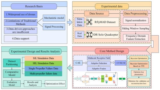
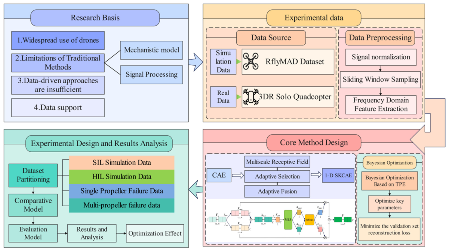
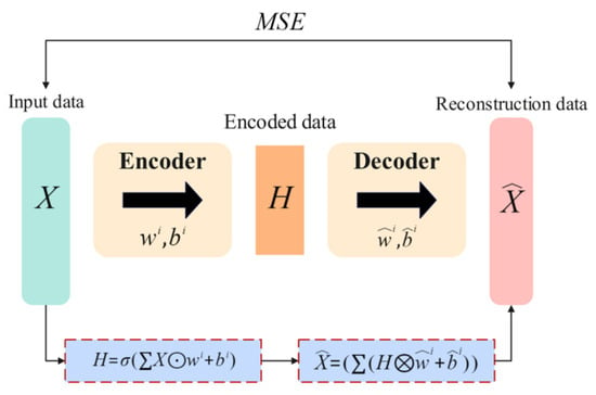
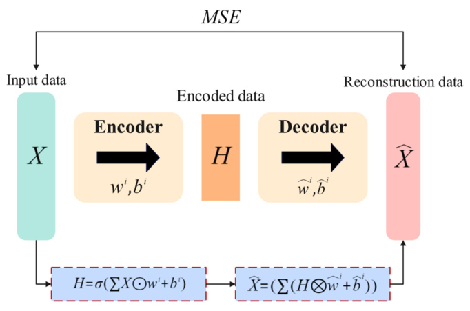
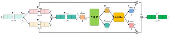
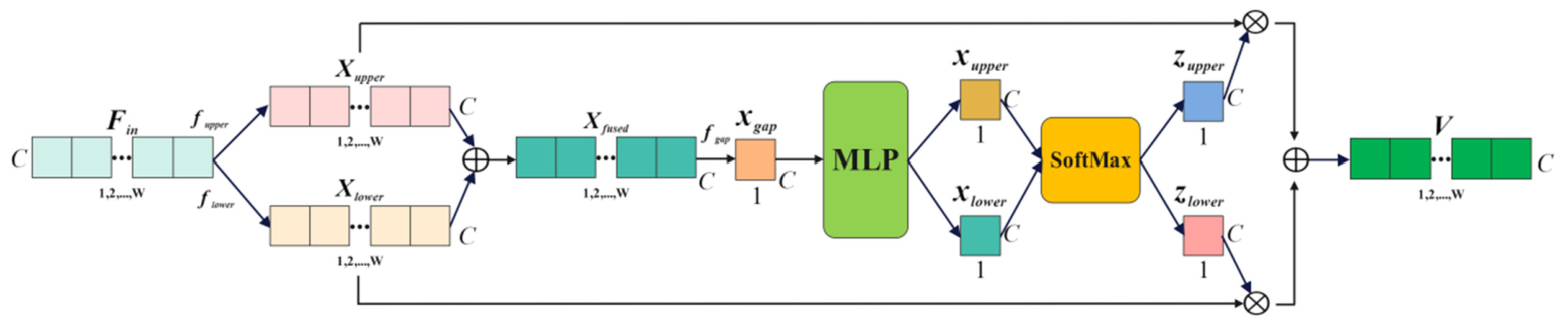
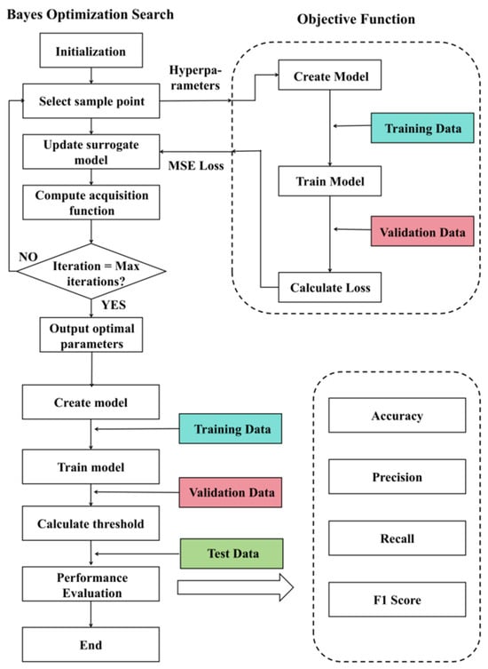
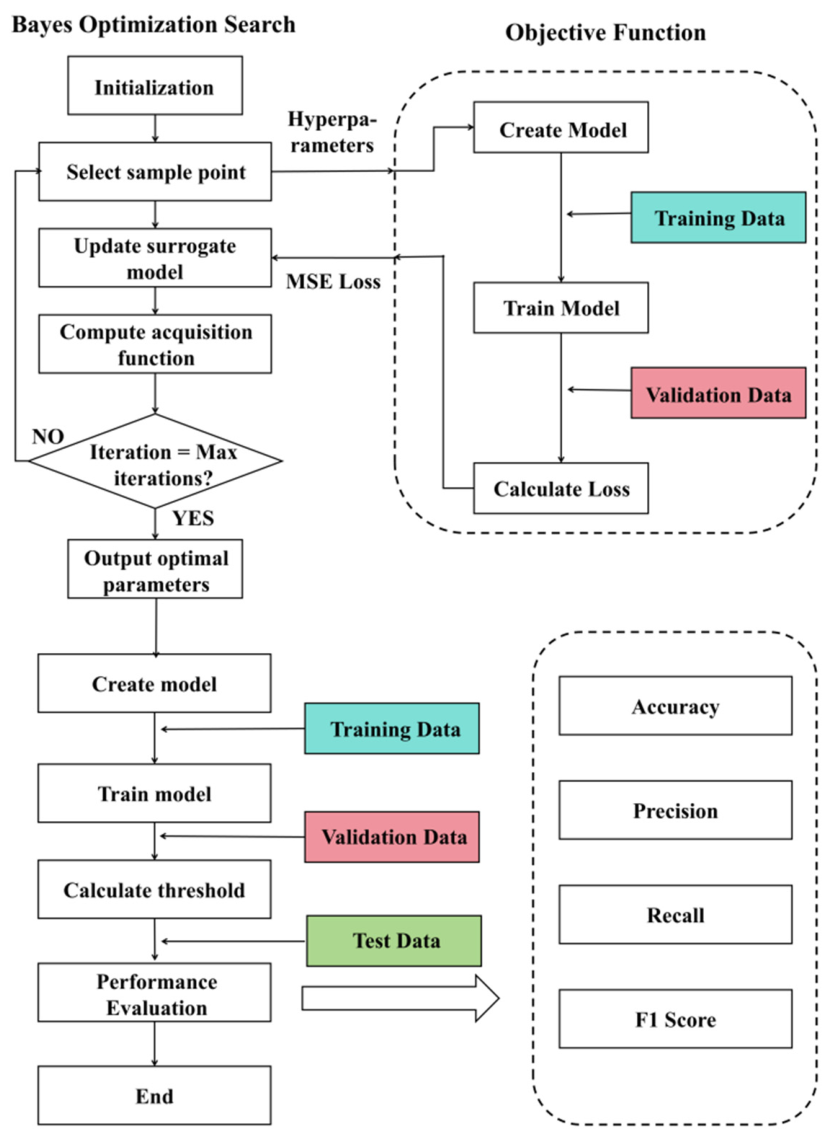
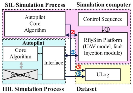
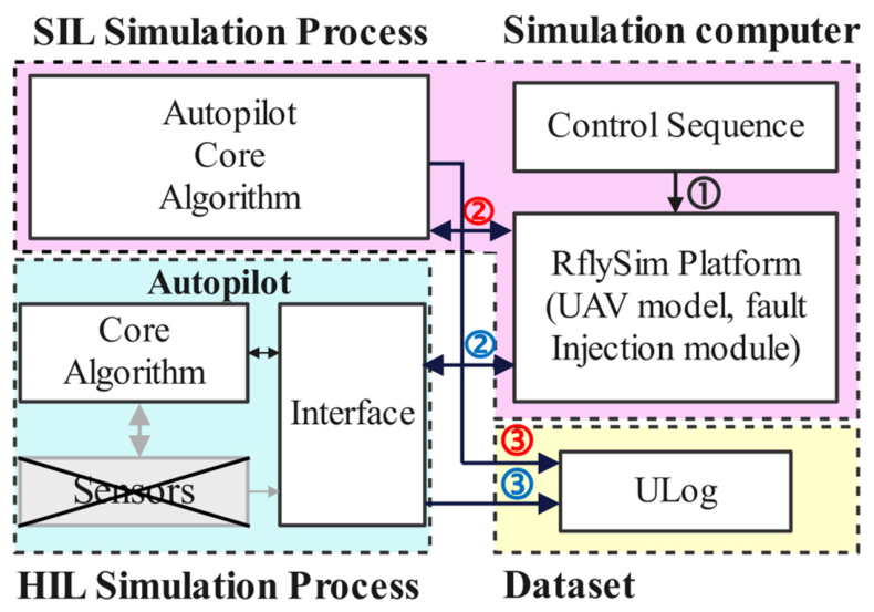
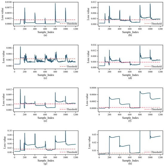
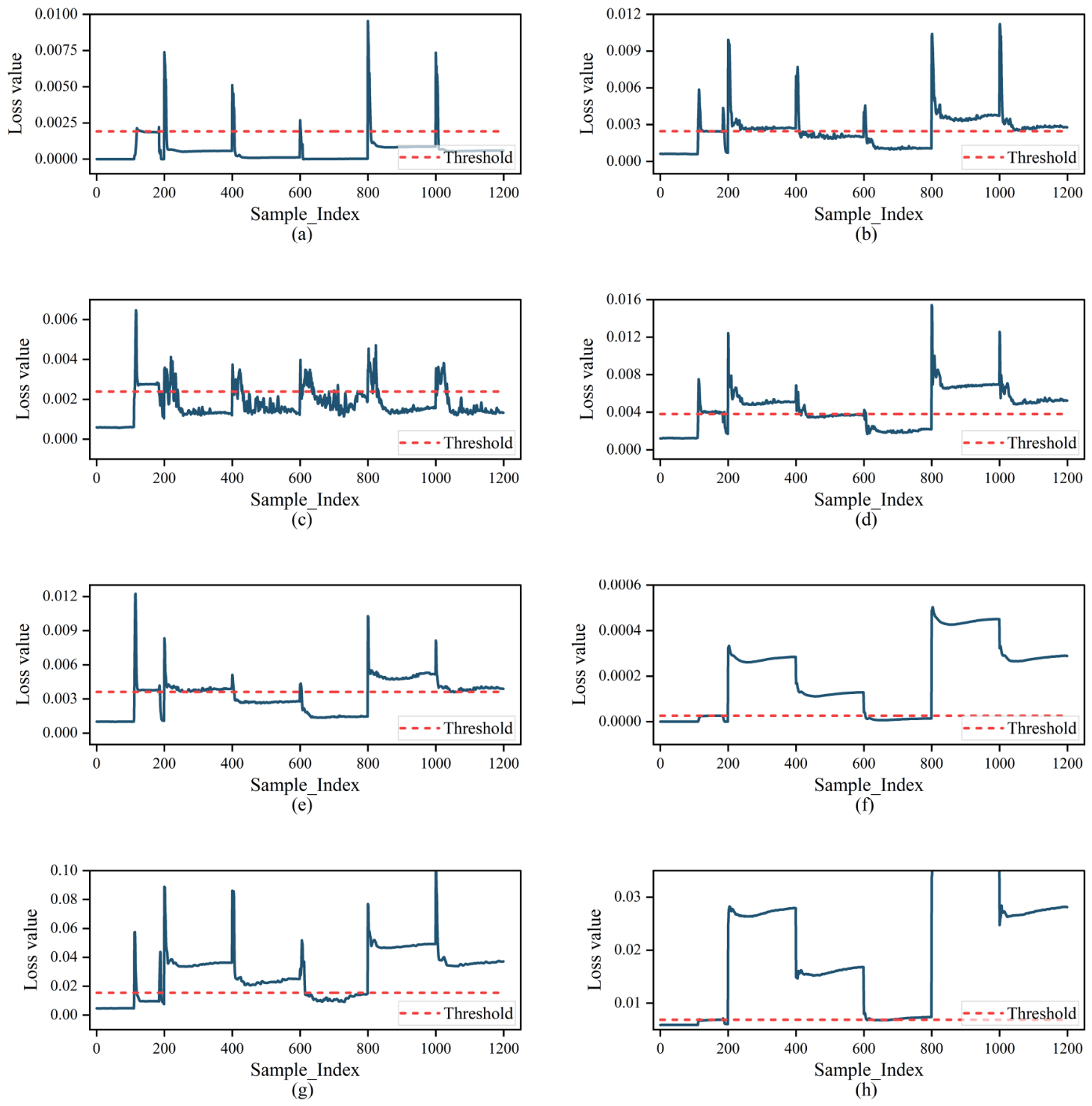
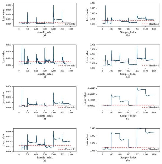
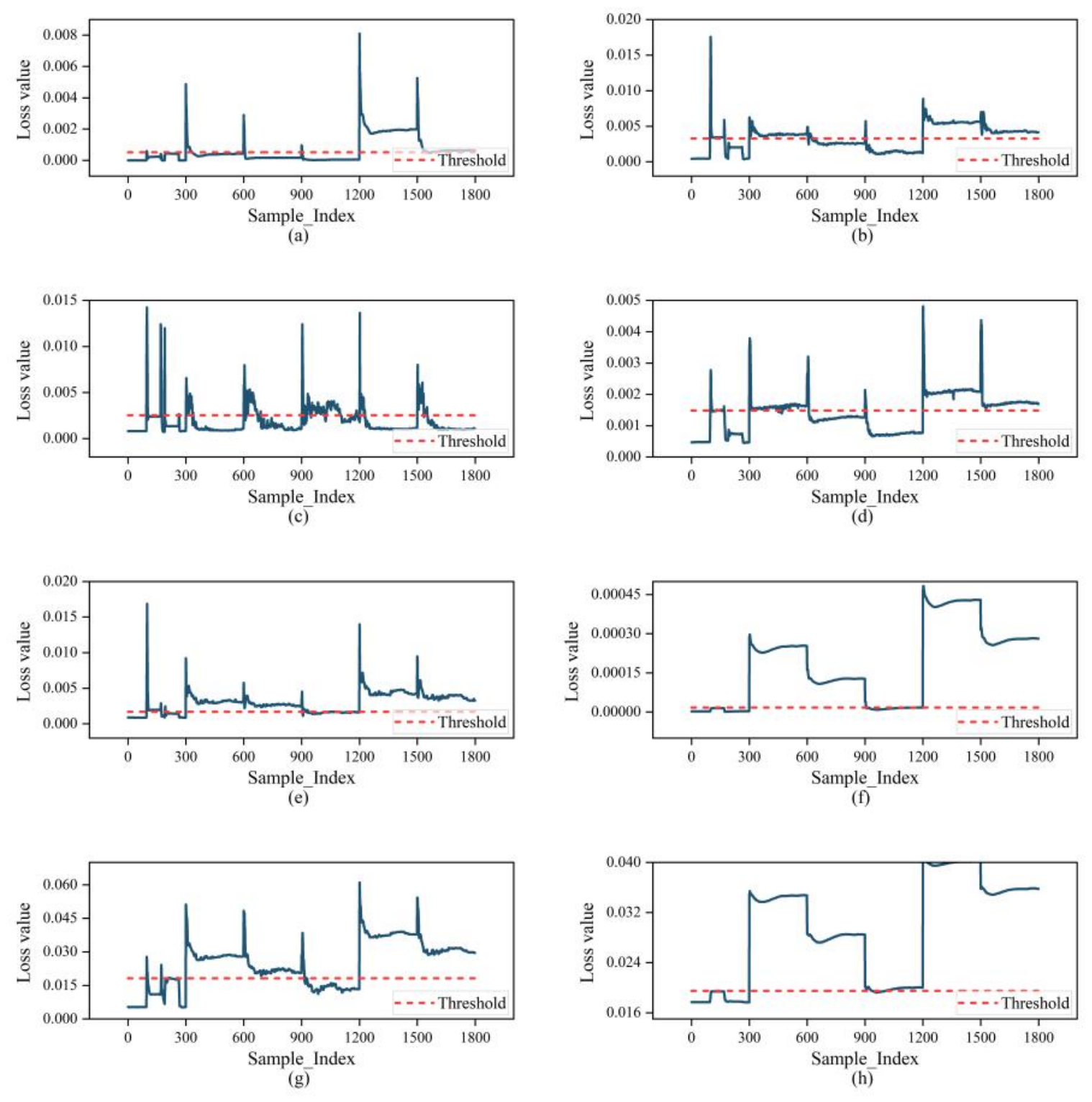
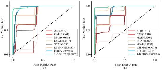
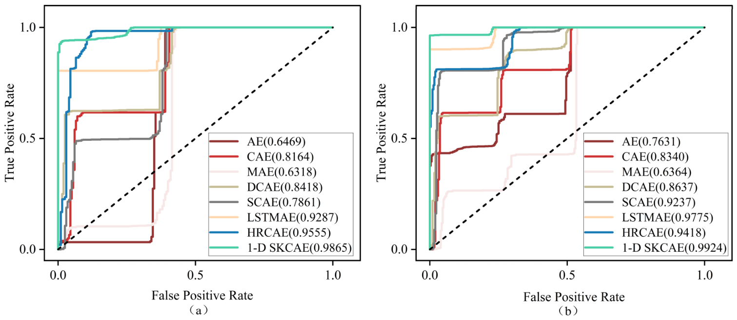
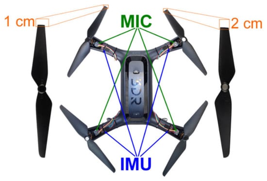
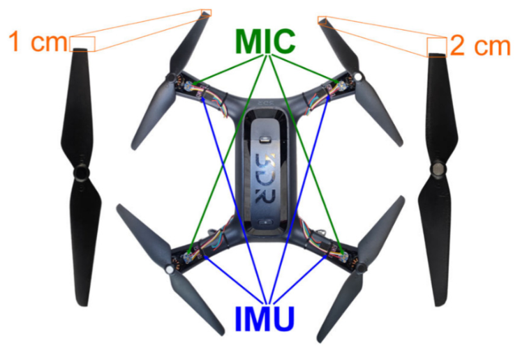
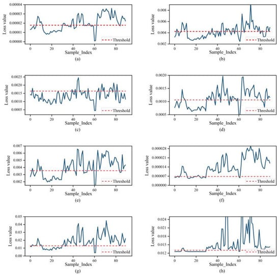
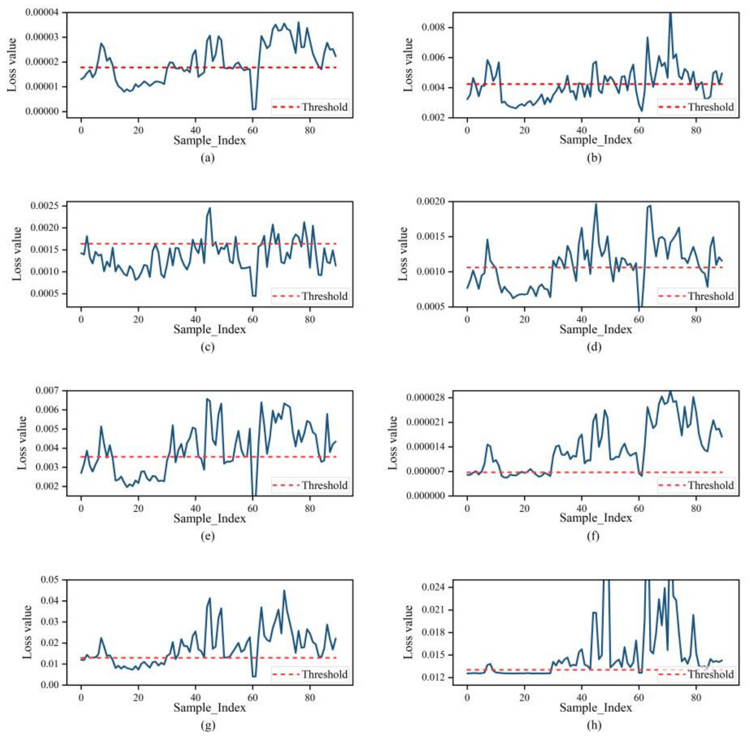
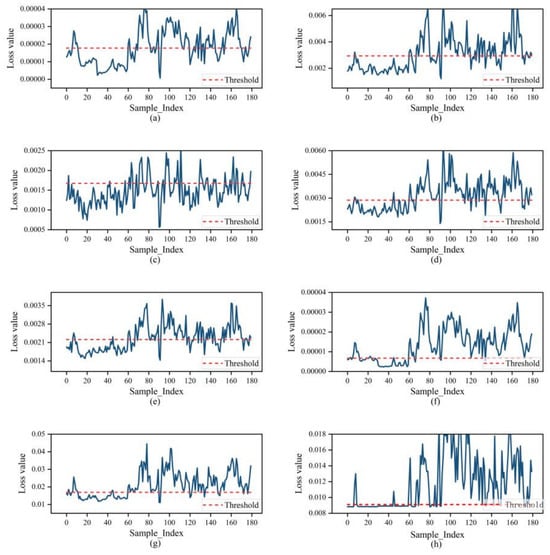
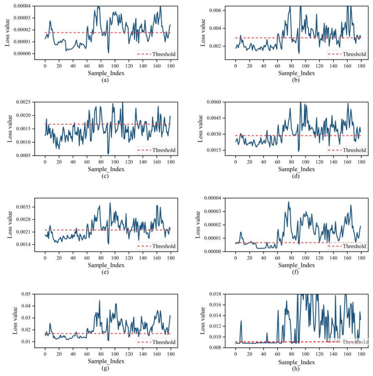
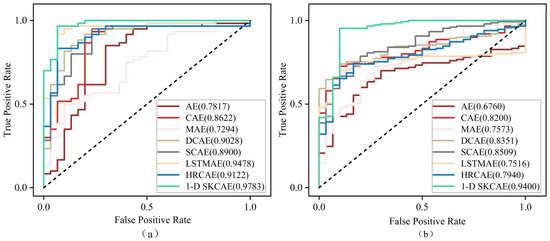
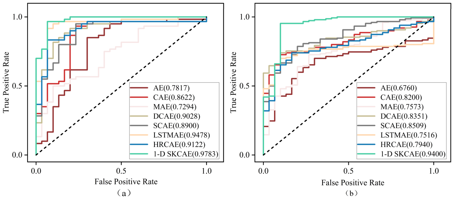
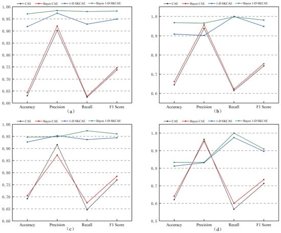
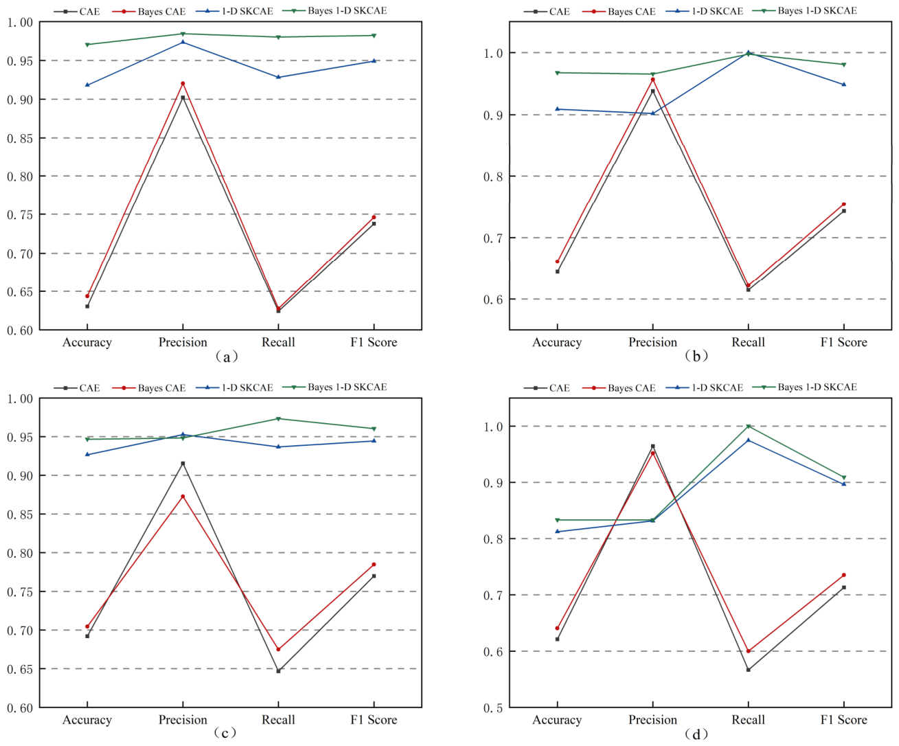
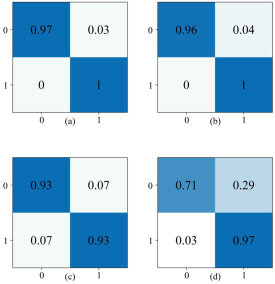
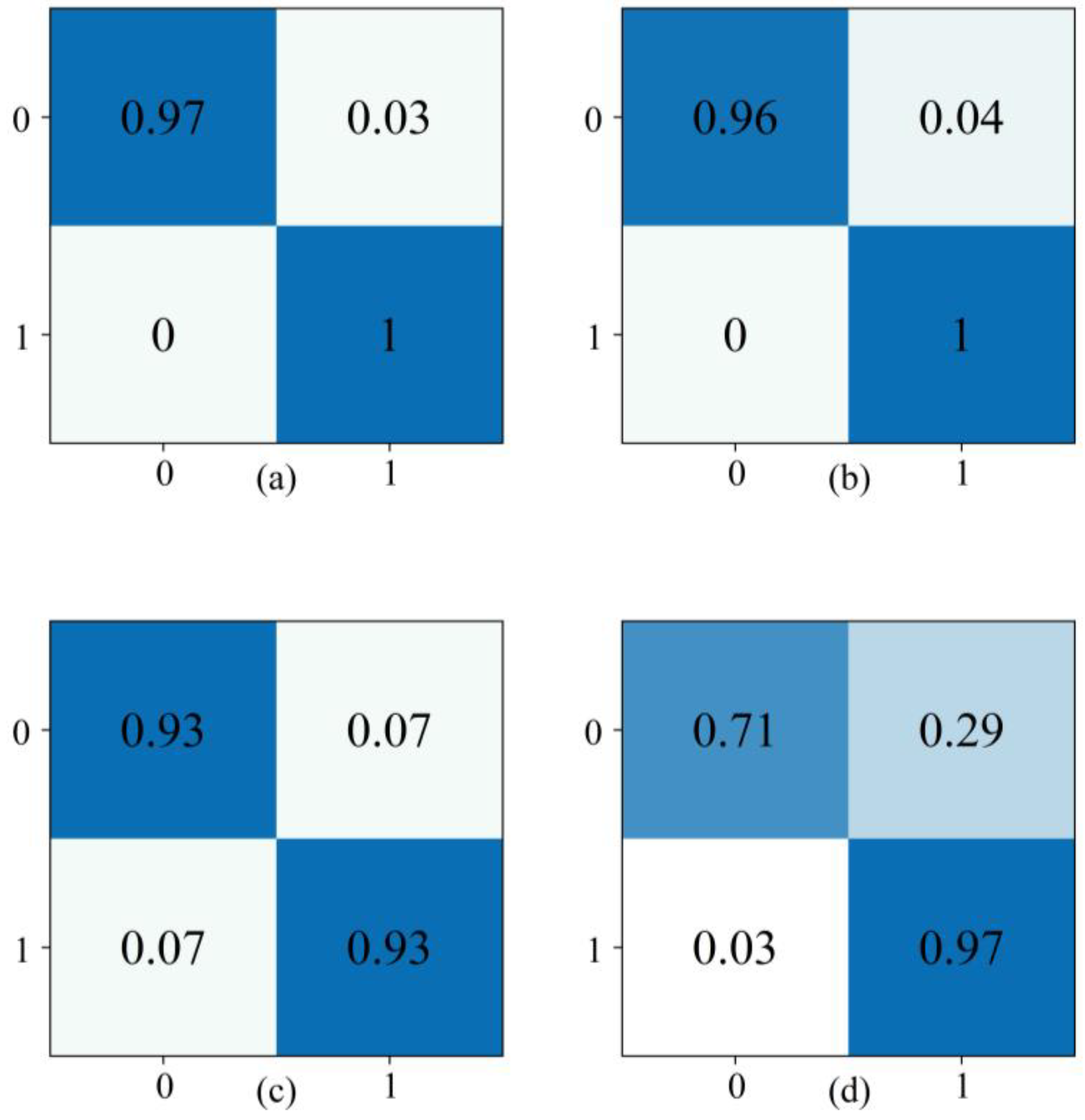

Disclaimer/Publisher’s Note: The statements, opinions and data contained in all publications are solely those of the individual author(s) and contributor(s) and not of MDPI and/or the editor(s). MDPI and/or the editor(s) disclaim responsibility for any injury to people or property resulting from any ideas, methods, instructions or products referred to in the content. |
© 2026 by the authors. Licensee MDPI, Basel, Switzerland. This article is an open access article distributed under the terms and conditions of the Creative Commons Attribution (CC BY) license.