


Abstract
Stepper-motor-driven Selective Compliance Assembly Robot Arms are susceptible to motion control challenges under short-stroke and high-frequency start–stop conditions, including high sensitivity to pulse timing, difficulty in multi-joint coordination, and insufficient trajectory smoothness. To address these issues, this paper proposes an optimized motion control method for smooth execution of obstacle-avoidance trajectories, integrating path smoothing, asymmetric S-curve velocity planning, and pulse-frequency-based multi-axis synchronization. First, piecewise cubic Hermite interpolation, Gaussian smoothing, and end-effector-based equidistant resampling are applied to post-process Rapidly-exploring Random Tree-generated paths, thereby eliminating polyline turning points and improving uniformity of waypoint distribution. Second, an asymmetric S-curve velocity planning method with nonzero boundary velocity constraints is developed, and multi-axis synchronization is achieved based on the maximum segment duration principle. Finally, instantaneous reference velocities are converted into per-axis pulse frequency commands via proportional mapping, enabling real-time stepper motor drive control. Experimental results show that the proposed method reduces the obstacle-avoidance path length by 8.52% and significantly decreases the dispersion of trajectory step sizes. In single-segment dynamic simulations, the proposed method reduces the peak dynamic output force by 62%. In real robot experiments, the average motion time across three obstacle-avoidance tasks is reduced by approximately 55.21%, while end-effector trajectory continuity and inter-joint coordination are improved, suggesting the effectiveness and preliminary engineering feasibility of the proposed method under the tested conditions.
1. Introduction
1.1. Background and Motivation
With the ongoing advancement of industrialization and the increasing adoption of automated production, industrial robots have been deployed across a growing range of manufacturing scenarios, particularly in assembly, dispensing, material handling, sorting, and precision insertion tasks [1,2,3]. As an important branch of robotics, industrial robots draw on mechanical engineering, electrical engineering, computer science, and artificial intelligence, integrating advances from many of these fields. Consequently, industrial robots not only enable operations in hazardous environments and reduce labor costs, but also ensure consistent product quality and significantly improve production efficiency [4,5].
As a representative class of industrial robots, the Selective Compliance Assembly Robot Arm (SCARA robot) plays a significant role in manufacturing automation upgrading due to its wide applicability, operational simplicity, and high system integrability. The SCARA robot is a planar articulated manipulator consisting of three revolute joints arranged in parallel and one prismatic joint along the vertical axis. This kinematic configuration provides selective compliance in the X–Y plane while maintaining high stiffness in the Z direction, thereby enabling high-speed and high-precision motion across a wide workspace [6,7,8]. Accordingly, SCARA robots have been widely adopted across industries such as 3C electronics, wafer fabrication, lithium-ion batteries, photovoltaics, and printing and packaging, playing a critical role in handling, assembly, dispensing, hot-pressing, screw fastening, and labeling.
As SCARA robots are increasingly deployed in complex tasks such as intelligent perception, precision assembly, and real-time operation, their working conditions are evolving toward higher cycle rates, greater precision, and more frequent start-stop cycles, making motion control performance a decisive factor in overall system efficiency and operational quality [9,10]. Existing studies on industrial robot motion planning and control have largely been developed under the assumption of long-stroke motion. When applied to short-stroke motion in SCARA robots, however, conventional trajectory planning methods are often unsuitable for direct deployment. On the one hand, the limited displacement often forces deceleration to begin before the prescribed peak velocity is reached, resulting in a compressed or even degenerate velocity profile. On the other hand, retaining fixed velocity, acceleration, and jerk parameters leads to trajectory distortion, which may further degrade into a triangular profile or an incomplete S-curve, causing insufficient deceleration, increased end-point impact, and degraded motion performance. These results indicate that motion control under short-stroke conditions cannot be achieved by simply scaling conventional long-stroke trajectory planning methods.
Moreover, such trajectory degeneration not only undermines planning accuracy but also induces a series of coupled issues at the levels of structural dynamics and actuation. For SCARA robots, these issues are not merely due to insufficient velocity planning accuracy, but fundamentally represent an electromechanical-coupled control problem involving interactions between system dynamics and actuator characteristics [11,12]. To satisfy the demands of high-speed, high-frequency operation, SCARA arms typically adopt lightweight link structures. While such designs enhance motion responsiveness, they also render the system more susceptible to high-order dynamic excitation under frequent start-stop and large acceleration/deceleration conditions, thereby increasing the risk of structural vibration and response distortion [13,14,15].
Meanwhile, in SCARA systems driven by stepper motors, short-stroke, high-speed motion control is further constrained by strict actuator limitations, particularly the significant torque–frequency characteristic, in which output torque decreases as pulse frequency increases [16,17]. Compared with servo motor systems, stepper motors still offer broad application potential in small- and medium-scale SCARA robots and lightweight automation equipment due to their simple structure, lack of encoder requirements, and low cost. However, inherent issues such as torque–frequency attenuation, open-loop discrete control, and difficulty in multi-axis coordination make them prone to missed steps, overshoot, and cumulative positioning errors when subjected to rapid acceleration changes during frequent start–stop operations. Therefore, the design of a rational and effective control algorithm that improves both the precision and stability of stepper motors under short-stroke, high-speed conditions is essential to enabling efficient and accurate operation of low-cost SCARA robots.
To address the above challenges, this study focuses on a low-cost stepper-motor-driven SCARA robot and proposes a collaborative motion control method spanning from path preprocessing and velocity planning to pulse execution. The scientific contribution of this work is not a new interpolation algorithm or a new general-purpose velocity profile, but a velocity-planning and execution method targeting the failure mode that governs step loss in open-loop stepper-based continuous obstacle-avoidance execution, namely abrupt and unbounded pulse-frequency transitions at intermediate waypoints. Its core elements are nonzero boundary-velocity constraints, an asymmetric seven-segment S-curve, and a closed-form peak-velocity solution, achieved through per-axis, independent frequency trajectories with a unified segment duration. The proposed method is motivated by small-scale automation scenarios and shows potential for low-cost SCARA motion control under short-stroke and high-frequency start-stop conditions. It also provides a methodological reference for motion planning problems in similar stepper-motor-driven robotic systems.
The remainder of this paper is organized as follows. Section 2 presents the proposed method, including joint-space path smoothing and equidistant resampling, pulse-space mapping and multi-axis synchronization, asymmetric seven-phase S-curve velocity planning, and time-domain pulse-frequency generation. Section 3 describes the experimental evaluation setup, including the experimental platform, motor, and driver specifications, and experimental design parameters. Section 4 reports the results and analysis of the geometric evaluation, dynamic simulation, ablation experiments, and physical experiments. Section 5 discusses the main findings, assumptions, and limitations. Section 6 concludes the paper and outlines future work.
1.2. Related Research
A targeted literature review was conducted to position the proposed method with respect to existing trajectory planning and motion execution studies. The reviewed studies were selected according to their relevance to industrial robot trajectory planning, S-curve and trapezoidal velocity profiles, stepper-motor or pulse-level motion control, and multi-axis synchronization. The selected studies were then analyzed using a feature-based comparison method, focusing on target platform, path preprocessing, velocity profile, jerk continuity, nonzero boundary velocity, multi-axis synchronization, pulse-level execution, and validation type.
In recent years, a growing body of research has focused on the industrial applications and intelligent extension of SCARA robots [18]. Rigatos et al. [19] proposed a nonlinear optimal control framework for a four-degree-of-freedom (4-DOF) SCARA manipulator, based on H-infinity optimal control combined with Taylor series linearization, thereby establishing a systematic theoretical basis for SCARA dynamic control. Huang et al. [20] developed an Active Force Control (AFC)-based strategy for trajectory tracking of SCARA robots under external disturbances, and validated its effectiveness in terms of disturbance rejection and tracking accuracy on a real robot platform. Kumar et al. [21] tackled the challenge of synchronizing trajectory planning and obstacle avoidance for Revolute–Revolute–Prismatic (RRP)-type SCARA robots in complex environments by proposing a fuzzy-logic-based coordination strategy, which effectively eliminates singularity issues and ensures safe manipulator operation. These studies provide important references for SCARA robot control, but they mainly focus on dynamic control, disturbance compensation, trajectory tracking, or path planning rather than low-level pulse-frequency execution for open-loop stepper-motor-driven SCARA robots.
Classical trajectory planning methods include trapezoidal and extended trapezoidal velocity profiles [22], cubic and quintic polynomial interpolation [23], S-curve planning [24], jerk-limited trajectory [25], and spline-based methods such as B-spline [26]. Trapezoidal velocity planning has been widely adopted owing to its simple implementation and low computational cost, and it is commonly used together with S-curve profiles as a standard trajectory interpolation scheme in motion-axis servo control [27]. However, the trapezoidal algorithm suffers from abrupt acceleration changes during start-stop phases, which produce flexible impacts and fail to effectively mitigate step loss and overshoot [28,29]. These issues become more pronounced in short-stroke multi-waypoint trajectories, where frequent acceleration and deceleration dominate the motion process.
To overcome the impact and vibration caused by acceleration discontinuities, S-curve acceleration/deceleration algorithms have been widely studied [30]. Wu et al. [31] developed a cubic-polynomial-based improved S-curve flexible acceleration/deceleration scheme for intelligent live-working robots, employing a five-segment motion-planning structure to achieve continuous acceleration control. Liu et al. [32] showed that, compared with trapezoidal and exponential acceleration/deceleration profiles, the S-curve achieves a more favorable trade-off between control complexity and positioning accuracy in high-precision servo motion control. Shen et al. [33] developed an FPGA-based S-curve acceleration/deceleration control module for numerical-control systems, focusing on hardware implementation and pulse generation. Li et al. [34] studied a five-segment S-curve acceleration/deceleration algorithm for gantry robots and discussed its advantages in short-stroke scenarios.
Although these studies have improved trajectory smoothness and acceleration/ deceleration continuity, many of them are developed under assumptions that are not fully consistent with low-cost open-loop stepper-motor-driven SCARA robots. For example, some methods assume servo feedback or dedicated hardware platforms, some mainly consider single-axis or point-to-point motion, and some use zero boundary velocity at each segment endpoint, which may lead to unnecessary intermediate stops in multi-waypoint obstacle-avoidance execution. In addition, path preprocessing, waypoint boundary velocity planning, asymmetric acceleration/deceleration constraints, multi-axis synchronization, and pulse-frequency execution are often treated as separate issues rather than as a coupled execution chain.
To clarify the relationship between the proposed method and existing studies, Table 1 compares representative velocity planning and trajectory execution methods from the aspects of target platform, path preprocessing, velocity profile, jerk continuity, nonzero boundary velocity, multi-axis synchronization, pulse-level execution, and validation. As shown in Table 1, the existing studies have made important contributions to time-optimal polynomial planning, S-curve smoothing, trapezoidal-profile-based vibration suppression, servo closed-loop control, and FPGA-based pulse generation. However, most of these methods focus on one or two aspects of the trajectory execution process, while the coupling among path preprocessing, velocity parameterization, multi-axis synchronization, and low-level pulse execution is less frequently addressed, especially for low-cost open-loop stepper-motor-driven SCARA robots.
Table 1.
Comparison of related velocity planning and trajectory execution methods.
1.3. Problem Formulation
Based on the above review, existing methods still have several limitations for short-stroke multi-waypoint obstacle-avoidance execution in open-loop stepper-motor-driven SCARA robots. Classical velocity planning methods are often designed for long-stroke or point-to-point motion, and fixed velocity, acceleration, and jerk parameters may result in compressed or degenerate profiles under limited displacement conditions. Although S-curve-based methods improve motion smoothness, many of them still assume zero boundary velocity at segment endpoints, which may cause unnecessary intermediate stops and reduce execution efficiency in continuous multi-waypoint trajectories. Moreover, path smoothing, velocity profile design, multi-axis synchronization, and pulse generation are often treated separately, while these factors are strongly coupled in pulse-based stepper motor execution. Therefore, a geometrically feasible path may still produce abrupt pulse-frequency transitions or poor inter-joint coordination if the entire execution chain is not considered jointly.
Accordingly, the problem addressed in this study can be formulated as follows. Given a collision-free but geometrically irregular multi-waypoint obstacle-avoidance path produced using a Rapidly-exploring Random Tree (RRT) planner, the objective is to transform it into smooth, synchronized, and pulse-executable multi-axis commands for a low-cost open-loop stepper-motor-driven SCARA robot. The generated commands should reduce abrupt pulse-frequency transitions at intermediate waypoints, maintain feasible acceleration and deceleration behavior within the motor torque–frequency constraints, and improve end-effector trajectory continuity without relying on encoder-based feedback or changing the hardware platform.
This problem formulation assumes that the input RRT path is already collision-free and that the obstacle layout remains unchanged during execution. The motor torque–frequency characteristics are considered known for determining feasible velocity and acceleration/deceleration limits. The system is also assumed to operate under open-loop pulse control, and the gripper joint is excluded from the main trajectory generation because it does not affect the primary end-effector motion.
Therefore, this study focuses on an execution-oriented problem rather than a general path planning or fully online replanning problem. The aim is to bridge the gap between feasible but irregular obstacle-avoidance paths and physically executable stepper-motor pulse commands by jointly considering path regularization, waypoint boundary velocity planning, asymmetric S-curve parameterization, segment-level synchronization, and pulse-frequency generation.
2. Methodology
2.1. Preliminaries
Before presenting the proposed method, this section briefly introduces the kinematic model and the mathematical tools on which the subsequent derivations rely.
Kinematic model. The SCARA robot considered in this study is a planar articulated manipulator with three revolute joints and one prismatic joint. Its forward kinematics, which maps the joint configuration to the end-effector position in task space, is described using the Denavit–Hartenberg (D–H) convention.
Raw path generation. The obstacle-avoidance paths processed in this work are feasible paths generated by RRT planner. RRT incrementally builds a search tree by random sampling in the configuration space and returns a collision-free but geometrically irregular sequence of waypoints. Path generation itself is not the focus of this study, and the RRT output is treated as the input trajectory to be post-processed.
Mathematical tools. Two tools are mainly used for path post-processing. The first is the PCHIP, a shape-preserving cubic interpolation that maintains the local monotonicity of the original data and suppresses the overshoot commonly associated with high-order splines. The second is Gaussian smoothing, a convolution-based low-pass filter that attenuates local high-frequency fluctuations while preserving the overall shape of the trajectory. In addition, arc-length parameterization is adopted to describe the trajectory, in which the cumulative Euclidean distance along the end-effector path is used as the parameter, thereby characterizing the geometric distribution of the trajectory in task space independently of the joint-space sampling.
2.2. Overview of the Proposed Framework
The overall framework of the proposed velocity control method for the stepper-motor-driven SCARA robot is shown in Figure 1. The framework takes a joint-space obstacle-avoidance path as input and sequentially processes it through four functional modules to generate and execute motion commands. Module 1 performs redundant point removal, arc-length parameterization, Gaussian smoothing, and equidistant resampling on the raw path, outputting a geometrically regularized sequence of N equidistant waypoints. Module 2 performs inter-axis mapping and dominant-axis identification in pulse space, and determines the non-zero or zero boundary velocity at each waypoint through a look-ahead initialization mechanism, thereby providing the constraint basis for multi-axis synchronization. Module 3 solves the asymmetric seven-segment S-curve velocity parameters in real time based on per-segment displacements and the torque–frequency constraints of the stepper motors, and outputs the complete segment durations and velocity functions. Module 4 computes the pulse period for each axis in real time from the velocity functions, generates direction signals and step-pulse sequences, and drives all joints in coordinated motion. By directly transmitting the complete S-curve parameters to the embedded execution layer, the proposed framework ensures consistency between the planning model and the low-level execution process, thereby improving trajectory smoothness and timing accuracy during motion execution.
Figure 1.
Hierarchical control framework for the stepper-motor-driven SCARA robot based on an asymmetric S-curve profile.
2.3. Joint-Space Path Smoothing and Equidistant Resampling
The raw obstacle-avoidance path is typically generated using RRT-based methods. Although such paths satisfy feasibility requirements, they often exhibit polyline turning points, non-uniform waypoint distribution, and localized abrupt variations at the discrete waypoint level. If directly applied to subsequent stepper motor control, these characteristics tend to induce non-smooth pulse frequency transitions during waypoint switching. Post-processing of sampling-based paths has been shown to markedly improve waypoint uniformity and continuity [35]. Therefore, prior to temporal parameterization of the trajectory, it is necessary to first perform smoothing and uniform resampling on the raw path.
Let the raw joint-space path be defined by Equation (1).
where denotes the displacement of the prismatic joint, , , and denote the angles of the three revolute joints.
First, consecutive duplicate points are removed to prevent degenerate intervals from arising during path parameterization. Subsequently, the position of the end-effector in task space, , is computed via forward kinematics, and the cumulative arc length along the path is defined using the Euclidean distance between consecutive end-effector positions, as shown in Equation (2).
where denotes the cumulative displacement of the end-effector along the spatial trajectory.
In the path smoothing stage, the cumulative arc length is first used as the interpolation parameter, and shape-preserving PCHIP is applied to the discrete joint-space path to generate a dense continuous trajectory. PCHIP preserves the local shape characteristics of the raw path and effectively suppresses the overshoot behavior commonly associated with high-order splines, making it particularly suitable for the continuous reconstruction of feasible obstacle-avoidance paths. On this basis, Gaussian smoothing is applied to the dense trajectory to attenuate jagged fluctuations and sharp angular variations in the raw RRT path, thereby improving trajectory continuity and local smoothness. To ensure positional accuracy at the task start and end points, an endpoint-preservation constraint is imposed on the smoothed trajectory, which enforces that the first and last endpoints of the smoothed path coincide exactly with those of the raw path, thereby preventing endpoint drift introduced by the smoothing process.
The choice of the above preprocessing techniques is mainly motivated by the geometric characteristics of RRT-generated paths and the trajectory execution requirements of stepper-motor-driven SCARA robots. Since the raw RRT path already satisfies the collision constraints, the goal of post-processing is not to re-plan the trajectory but to improve continuity while preserving obstacle-avoidance feasibility. To this end, PCHIP cubic interpolation is adopted for its shape-preserving property, which maintains the local variation tendency of the discrete path and avoids the overshoot that natural cubic splines or high-order polynomials may produce in sharp turning regions; then Gaussian smoothing is applied to attenuate, at relatively low computational cost, the local jagged fluctuations of randomly sampled RRT paths; finally, since the nonlinear forward kinematics of the SCARA robot causes uniform spacing in joint space or in the parameter domain to no longer correspond to uniform physical displacement in task space—on which the stability of the subsequent pulse-frequency modulation and multi-axis synchronization control directly depends—arc-length-based equidistant resampling in the end-effector Cartesian space is employed, thereby providing geometrically continuous and uniformly spaced trajectory inputs for the subsequent asymmetric S-curve velocity planning and pulse-frequency-based multi-axis synchronization control.
Since the smoothing operation alters the actual length distribution of the trajectory in task space, the end-effector path length corresponding to the smoothed trajectory must be recomputed via forward kinematics after smoothing is completed. Let denote the end-effector position corresponding to the i-th dense interpolated point of the smoothed trajectory. Its cumulative arc length can then be expressed by Equation (3):
Furthermore, the total physical arc length interval is uniformly divided into M sampling positions, as shown in Equation (4):
The smoothed joint-space trajectory is then resampled based on these uniformly distributed arc-length positions to obtain the final equidistantly resampled path, as shown in Equation (5):
2.4. Pulse-Space Mapping and Multi-Axis Synchronization for Stepper Motors
Since the embedded controller directly drives stepper motors, the joint-space trajectory must be further converted into discrete position commands in the motor pulse space. In the proposed system, joints , and are actuated by stepper motors, while the gripper joint is driven by a servo motor. Since does not contribute to the formation of the primary end-effector trajectory, pulse planning is performed only for the first three joints. Let the joint path after smoothing and equidistant resampling be defined by Equation (6):
According to the system calibration relationship, each joint variable is mapped to the corresponding target motor pulse position by Equation (7):
where , , and are the pulse scaling coefficients, , , and are the zero-position offsets, and is the mechanical coupling compensation term.
Since stepper motor actuation is inherently quantized into integer pulses, the mapped values must be discretized prior to control, yielding the pulse-space trajectory, as shown in Equation (8):
This step converts the continuous joint-space trajectory into discrete target positions directly executable by the low-level driver, establishing a unified foundation for subsequent velocity planning and pulse frequency generation.
As shown in Figure 2, in the pulse space, each pair of adjacent path points forms a discrete motion segment, and each segment contains the motion increments of the three robot joints. For the k-th segment, as shown in Equation (9):
Figure 2.
Discrete motion segments between path waypoints.
Unlike conventional approaches that apply uniform scaling based on a dominant axis, the proposed method adopts a strategy of independent per-axis waypoint velocity planning combined with segment-level time synchronization, tailored to the characteristics of multi-axis discrete stepper motor control. Specifically, an independent per-axis waypoint velocity sequence is established for each axis, where and , and these values serve as the velocity boundary conditions between adjacent segments. The core idea is to set the velocity of an axis to zero at a waypoint only when that axis undergoes a direction reversal. Otherwise, if the motion direction remains consistent across adjacent segments, the axis is allowed to maintain a nonzero transition velocity at the waypoint. This avoids the overly conservative case in which a reversal of a single axis forces simultaneous deceleration of all axes, thereby better matching the execution requirements of multi-axis stepper motor systems.
The determination of the waypoint velocity sequence consists of three stages. First, a look-ahead initialization procedure is performed. For an intermediate waypoint , if the displacement directions of the j-th axis remain consistent across two adjacent segments, the initial waypoint velocity is set to 90% of the maximum velocity limit of that axis, . If a direction reversal occurs between the adjacent segments, the waypoint velocity is forcibly set to zero, . The velocities at the starting and ending waypoints are always initialized to zero. Subsequently, a forward pass is performed by traversing the waypoints sequentially from waypoint 1 to waypoint N, during which an acceleration reachability constraint is imposed at each waypoint, as shown in Equation (10).
where denotes the acceleration limit of the j-th axis, and represents the pulse displacement of the preceding segment along the j-th axis. This constraint ensures that the waypoint velocity does not exceed the maximum reachable velocity attainable through acceleration from the previous waypoint.
Finally, a backward pass is performed by traversing the waypoints in reverse order from waypoint to waypoint 1, during which a deceleration reachability constraint is imposed, as shown in Equation (11):
where denotes the deceleration limit of the j-th axis, ensuring that the waypoint velocity can be reduced to satisfy the deceleration requirement within the subsequent segment.
After bidirectional envelope correction, the final waypoint velocity sequence satisfying the actual acceleration and deceleration capabilities of the stepper motors can be obtained. Accordingly, for the k-th segment of the j-th axis, the initial and terminal velocities are denoted by Equation (12):
2.5. Asymmetric Seven-Segment S-Curve Velocity Planning
In the execution of discrete obstacle-avoidance trajectories in SCARA robots, conventional trapezoidal velocity planning is prone to significant jerk excitation at waypoint transitions due to abrupt acceleration discontinuities [36]. Conventional S-curve methods typically assume zero velocity at both the start and end of each segment, making them ill-suited to the continuous transition requirement of multi-waypoint trajectories where the robot decelerates through corners without coming to a complete stop. To address this, this study adopts an asymmetric seven-segment S-curve velocity planning method with non-zero boundary velocity constraints to characterize the velocity evolution within a single discrete motion segment, serving as the fundamental time-parameterization unit for multi-segment stepper motor control.
As described in the previous section, the displacement of a given axis within the current segment is S, with initial and terminal velocities and , respectively. The maximum permissible velocity is set to based on motor performance, and the maximum acceleration and deceleration are and , respectively. Based on these parameters, a seven-segment S-curve trapezoidal velocity profile is adopted. During the acceleration phase, the velocity passes through three sub-phases: increasing acceleration, constant acceleration, and decreasing acceleration. During the deceleration phase, it passes through three corresponding sub-phases: increasing deceleration, constant deceleration, and decreasing deceleration. If the displacement is sufficient, a constant-velocity phase exists between the acceleration and deceleration phases. This velocity model permits , thereby naturally capturing the asymmetric dynamic characteristics of stepper motor systems, in which acceleration is typically gradual while deceleration is more aggressive. Accordingly, the characteristic jerk times of the acceleration and deceleration phases are denoted and , respectively, and the total acceleration and deceleration durations are given by Equation (13):
Given the boundary velocities and dynamic constraints, it is first necessary to determine whether the current segment is capable of reaching the maximum velocity . To this end, the critical displacement envelope required for full acceleration and deceleration is given by Equation (14):
If , the segment length is sufficient for the trajectory to reach the maximum velocity, in which case the peak velocity is set to and a constant-velocity phase exists. If , the segment is insufficient to support a complete acceleration–constant velocity–deceleration profile; the constant-velocity phase degenerates to zero duration, and the trajectory reduces to an asymmetric bell-shaped velocity curve. To ensure that the given boundary velocity constraints are satisfied within the finite displacement, the peak velocity is obtained analytically from the displacement balance relation in Equation (15):
This closed-form expression eliminates the need for iterative numerical solutions, allowing the velocity parameters of each segment to be determined directly, which is particularly well-suited to the pre-planning stage on the host computer, where real-time performance is critical.
After the peak velocity is determined, the characteristic jerk times of the acceleration and deceleration phases are given by Equation (16):
The total duration of the segment is therefore given by Equation (17).
where is the duration of the constant-velocity phase. When the trajectory degenerates to a bell-shaped curve, .
Based on these parameters, the intra-segment velocity function and acceleration function can be constructed, ensuring that the velocity evolves continuously throughout the discrete segment according to the seven-segment profile. Let the local time . The acceleration function is then given by Equation (18):
Correspondingly, the velocity function is given by Equation (19):
This formulation eliminates the acceleration discontinuities inherent in conventional trapezoidal planning while preserving continuous transition capability under non-zero boundary-velocity conditions. The per-axis S-curve parameter computation and velocity/acceleration reconstruction implemented in the current codebase are established directly upon the unified closed-form relations presented above.
2.6. Time-Domain Pulse-Frequency Generation for Stepper Motors
The fundamental control quantity of a stepper motor is the pulse sequence. Therefore, after obtaining the asymmetric S-curve trapezoidal velocity planning parameters for each axis, the proposed method does not transmit a continuous position trajectory directly to the embedded controller. Instead, the start and end pulse positions of each discrete motion segment, together with the corresponding per-axis velocity–acceleration–time parameters, are packaged and transmitted. During the execution phase, the embedded controller reconstructs the instantaneous reference velocity of each axis in the time domain in real time and generates the corresponding stepper pulses accordingly.
For a stepper motor, the physical interpretation of the velocity function is not merely the derivative of continuous displacement, but rather the number of pulses that should be output per unit time. If the instantaneous reference velocity of a given axis is , the corresponding pulse frequency is proportional to the velocity. Let the pulse resolution be denoted by K(pulse/unit), the relation is given by Equation (20):
Correspondingly, the pulse period is given by Equation (21):
This indicates that velocity planning in the continuous time domain, after proportional mapping, ultimately manifests as a pulse frequency modulation problem at the drive layer: higher velocity corresponds to denser pulses, lower velocity to sparser pulses, and continuously varying velocity produces correspondingly continuous variation in pulse frequency.
In multi-axis stepper motor control, the proposed method abandons the conventional approach of scaling all remaining axes to a single dominant-axis frequency and instead establishes an independent time-domain velocity function for each axis. Under the segment-level time synchronization condition, all three axes share a common local time reference. As a result, each axis maintains its own independent velocity boundaries and acceleration/deceleration characteristics, yet all axes reach their respective target positions simultaneously within the unified segment duration. The essence of this approach is that the time reference is unified, while the frequency trajectories of each axis remain independent. Consequently, even when different axes differ in displacement magnitude, boundary velocities, and dynamic capabilities, each axis generates its own distinct pulse frequency from its individual velocity function , thereby achieving coordinated multi-axis motion.
3. Evaluation
A four-axis SCARA robot was used as the experimental platform, as shown in Figure 3. In addition, the Denavit–Hartenberg method was adopted to describe the kinematic configuration of the SCARA robot, as listed in Table 2. The experimental setup also includes an Arduino Mega 2560 as the embedded controller board. The host computer used in the experiments was equipped with an AMD Ryzen 5 5600U CPU and an NVIDIA MX450 GPU.
Figure 3.
(a) SCARA robot structure; (b) D-H coordinate system.
Table 2.
SCARA robot linkage parameters.
The robot joints are driven by two-phase hybrid stepper motors (MS17HD4P4100, NEMA 17, MOONS’, Shanghai, China), with a step angle of 1.8° (200 steps/rev), a rated phase current of 1.0 A, a holding torque of 0.33 N·m, a phase resistance of 4.2 , and a phase inductance of 7.5 mH. The low-level drive adopts the Allegro A4988 module, with a motor supply voltage of 12 V and the phase current limit set to the rated value of 1.0 A. To improve the smoothness of low-speed motion and suppress mechanical resonance, the driver is configured in 1/16 microstepping mode (3200 steps/rev). Combined with a mechanical transmission lead of 20 mm/rev, the pulse resolution of the system is 160 pulses/mm. The complete specifications of the motor and driver are summarized in Table 3.
Table 3.
Specifications of the stepper motors and driver.
Since the proposed method is developed based on the physical limitations of stepper motors, Figure 4 presents the torque–frequency characteristic curve of the MS17HD4P4100 motor under a 12 V supply voltage and a 1.0 A phase current. The output torque decreases significantly as the rotational speed increases, dropping from approximately 0.245 N·m in the low-speed range to about 0.0734 N·m at 600 rpm, and approaching the effective operating limit near 800 rpm. This pronounced torque–frequency attenuation is precisely the constraint addressed by the proposed method. In the experiments, the maximum joint pulse frequency is approximately 2000 Hz, corresponding to a motor speed of about 37.5 rpm, which lies in the low-speed region with sufficient torque (>0.2 N·m) and is far below the attenuation region. Therefore, all velocity and acceleration/deceleration parameters used in this study were selected within the safe operating range estimated from the motor torque–frequency characteristics. These parameter settings help reduce the risk of step loss under open-loop control.
Figure 4.
Torque–frequency characteristic curves of the motor under different supply voltages. The 12 V/1 A curve corresponds to the configuration used in this study.
4. Results
4.1. Path Optimization Effectiveness Experiment
To verify the practical effectiveness of the joint-space path smoothing and end-effector equidistant resampling method proposed in Section 2.3 for obstacle-avoidance trajectory optimization, and to comprehensively evaluate its adaptability and robustness in diverse industrial scenarios, this section conducts comparative re-optimization experiments on the original obstacle-avoidance paths generated using the RRT method. Six groups of experiments were designed in total (Test 1–Test 6), systematically covering different path lengths, obstacle layouts, waypoint densities, and clearance constraints. Among them, Test 1 and Test 2 correspond to short-stroke obstacle-avoidance paths with a single obstacle, where the original paths contain a relatively large number of waypoints but exhibit different distribution patterns. Test 3 represents a detour path with obvious local nonuniformity in waypoint density. Test 4 corresponds to a dense multi-obstacle scenario. Test 5 represents a long-stroke scenario, in which the original path length increases to approximately 0.72 m. Test 6 tightens the safety clearance requirement from 20 mm, as used in the other groups, to 10 mm, in order to examine the feasibility of the proposed method under more stringent clearance constraints. To provide a statistically reliable evaluation, each group of experiments was independently repeated five times based on random RRT sampling, and the mean, standard deviation, and 95% confidence interval for each metric were calculated. The deterministic post-processing pipeline substantially compresses the variance introduced by random RRT sampling; accordingly, formal statistical testing, effect-size analysis, and a justification of the five-trial sample size are provided in Supplementary Material S1. The comparative results before and after optimization for the six groups of paths are shown in Figure 5.
Figure 5.
Optimization effects of different obstacle-avoidance planned trajectories; (a) Test 1; (b) Test 2; (c) Test 3; (d) Test 4; (e) Test 5; (f) Test 6.
The left part of Figure 5 compares the distributions of the original path (red) and the optimized path (blue) in the three-dimensional workspace, while the lower part shows the variation in trajectory step size. Overall, while preserving the original obstacle-avoidance topology and safety margin, the optimized path significantly improves the uniformity of waypoint distribution. In Test 1 and Test 2, the original paths exhibit obvious waypoint clustering and abrupt changes in turning and step-transition regions, with local peaks in trajectory step size reaching 0.0469 m and 0.0604 m, respectively, which are significantly higher than the typical range of 0.005–0.01 m in the remaining segments. After applying the proposed method, the trajectory step size stably converges to approximately 0.012 m, with very small fluctuations throughout the entire path. In Test 3, the step size of the original path fluctuates sharply within the range of 0.001–0.02 m and exhibits high-frequency oscillations, whereas after optimization, the waypoint spacing is uniformly redistributed to approximately 0.02 m. In Test 4–Test 6, although the obstacle layouts are denser, the paths are longer, or the clearance constraints are stricter, the proposed method still effectively eliminates the local step-length peaks of the original paths. The optimized step size converges to a uniform level in all scenarios, indicating that the method has good adaptability to different obstacle environments.
To quantitatively evaluate the improvement in waypoint distribution uniformity before and after path optimization, this section adopts the standard deviation of trajectory step size, , as the main evaluation metric to characterize the degree of dispersion of step sizes along the entire trajectory. Meanwhile, the total path length is introduced as a supplementary metric for comprehensive comparison. In addition, to address the need for quantitative evaluation of obstacle-avoidance safety, the minimum obstacle clearance and safety margin are further introduced as safety metrics. The safety margin is defined as the minimum obstacle clearance minus the preset safety requirement: 20 mm for Test 1–5 and 10 mm for Test 6. A value below zero indicates a violation of the safety constraint. The statistical results of all metrics for the six groups of experiments are shown in Figure 6.
Figure 6.
Performance comparison between the original path and the optimized path under different obstacle avoidance experiments: (a) comparison of path total length; (b) comparison of the standard deviation of inter-waypoint distance; (c) comparison of minimum obstacle clearance; (d) comparison of safety margin.
Figure 6a presents the comparison of the total path lengths. After optimization, the average path length of all six groups is reduced by 8.52% compared with the raw paths, with the reduction being smaller in the short-stroke scenarios (Test 1 and Test 2) and more pronounced in the long-stroke scenarios; in particular, Test 5 is reduced from approximately 0.736 m to approximately 0.564 m. Overall, the reduction ratio of the path length increases with the raw path length. This is because PCHIP interpolation and Gaussian smoothing, while preserving the endpoint constraints and obstacle-avoidance feasibility, attenuate the polygonal inflection points and sharp angular discontinuities of the raw RRT path, so that the reduction in total length stems entirely from geometric corrections in the mid-trajectory region and introduces no additional detour risk.
As shown in Figure 6b, the step size standard deviation of the original paths reflects the inherent and significant discreteness in the inter-waypoint distances of paths generated by RRT. After optimization, the step-size standard deviation across all six groups is reduced by approximately one order of magnitude, and this reduction is consistent across different obstacle layouts, path lengths, and waypoint densities. Even in the long-stroke scenario with more waypoints and a larger workspace (Test 5), as well as in the dense multi-obstacle scenario (Test 4), the proposed method can still stably reduce the discreteness to the same order of magnitude, demonstrating good cross-environment generalization capability.
As shown in Figure 6c,d, regarding the minimum obstacle clearance and safety margin, the mean values of the minimum obstacle clearance before and after smoothing remain basically unchanged across all six groups, with no significant clearance degradation caused by geometric smoothing. Across all 30 experiments across the six groups, the minimum obstacle clearance after smoothing remains strictly positive, and the collision rate is 0, verifying that the proposed smoothing procedure maintains obstacle-avoidance feasibility across different obstacle environments and clearance constraints. It should be noted that, in Figure 6d, the lower bounds of the error bars for the safety margin after optimization in some experimental groups fall below zero. This is caused by the relatively wide confidence intervals under five repeated trials in each group and reflects statistical dispersion; it does not indicate actual collisions. To explicitly verify this, the absolute minimum obstacle clearance and the corresponding safety margin for all five repetitions in every group, both before and after smoothing, are reported in Supplementary Material S2. Notably, in Test 6, which has the most stringent clearance constraint, the mean safety margin after smoothing is approximately 0.061 mm, close to the 0.058 mm obtained by the original method. This indicates that geometric smoothing does not lead to a significant reduction in safety margin even under narrow-clearance conditions.
In summary, while preserving the original endpoints and obstacle-avoidance feasibility, the proposed joint-space path smoothing and equidistant resampling method significantly improves waypoint uniformity, moderately shortens the end-effector travel distance, and maintains stable safety clearance under different obstacle environments. This method provides discretized inputs with consistent step size and smooth geometry for subsequent pulse-space mapping, waypoint velocity look-ahead, and asymmetric S-curve/trapezoidal acceleration–deceleration planning, thereby laying the foundation for synchronized segmented execution of multi-axis stepper motors.
4.2. Single-Segment Dynamic Simulation of the Stepper Motor and Comparative Analysis of Acceleration/Deceleration Algorithms
To evaluate the dynamic performance of the proposed asymmetric S-curve profile in single-segment stepper motor motion, comparative simulations were performed between the conventional trapezoidal velocity planning method and the proposed asymmetric S-curve trapezoidal method. The simulated motion was limited to a single segment between two adjacent discrete waypoints, without path look-ahead or multi-segment concatenation, in order to highlight the direct influence of different acceleration/deceleration strategies on the dynamic response of the stepper motor. The simulated motor parameters were derived from the physical characteristics of a standard NEMA 17 hybrid stepper motor with a 1.8° step angle driving a linear transmission mechanism. With a typical 16-microstep configuration and a transmission lead of 20 mm/rev, the spatial pulse resolution was calculated as 160 pulse/mm. The equivalent translational mass of the load was set to 1.0 kg. In the simulation program, the simulation time step was set to s, and the single-segment displacement was divided into a short-stroke motion of 5 mm and a longer-stroke motion of 20 mm. The maximum velocity was set to 12.5 mm/s for both methods. For the asymmetric S-curve method, the acceleration and deceleration were set to 50 mm/s2 and 100 mm/s2, respectively, whereas both the acceleration and deceleration of the conventional trapezoidal method were set to 50 mm/s2.
Figure 7 presents the velocity, acceleration, jerk, and dynamic output force responses of the two methods under the short-stroke condition. Under the short-stroke condition, the motion profile is dominated by the acceleration and deceleration phases, so the system response is primarily determined by the start-stop transition. In the conventional trapezoidal method, the acceleration undergoes abrupt discontinuities at the onset of acceleration and at the switching point to deceleration, leading to a theoretical impulsive jerk response. In contrast, the asymmetric S-curve method introduces a gradual acceleration transition during both the acceleration and deceleration phases, ensuring continuity of the acceleration profile and significantly suppressing the peak jerk. As shown in Table 4, under the sampling interval of , the peak jerk of the conventional trapezoidal method reaches , whereas that of the asymmetric S-curve method is only . However, since the acceleration of the trapezoidal profile contains discontinuities at the switching instants, its jerk is theoretically impulsive. Therefore, the numerically calculated peak jerk is strongly dependent on the sampling interval used in the simulation. For example, when the sampling interval decreases from to , the peak jerk of the trapezoidal method increases from approximately to . In contrast, the asymmetric S-curve method maintains a continuous acceleration profile, and its jerk value remains stable under different sampling intervals. Therefore, the peak jerk of the trapezoidal method is provided only as a reference, and the sampling-independent dynamic output force is adopted as the primary metric. The peak and Root Mean Square (RMS) dynamic output forces of the conventional trapezoidal method are 2.63 N and 0.25 N, respectively, while those of the S-curve method are reduced to 0.99 N and 0.16 N, corresponding to reductions of approximately 62% and 37%. As these forces are directly proportional to the actual motor-side acceleration, they equivalently characterize the measured acceleration response. These results indicate that under short-stroke, start-stop-dominated conditions, the S-curve method substantially reduces both transient impact and average force levels, thereby mitigating the risks of step loss, mechanical resonance, and thermal accumulation. Although the total motion time increases slightly from 0.63 s to 0.67 s, the dynamic stability is significantly improved.
Figure 7.
Simulation comparison of two stepper motor velocity control methods under short-stroke motion: (a) velocity response; (b) acceleration response; (c) jerk response; (d) dynamic output force response.
Table 4.
Simulation results of the two velocity planning methods for stepper motor short-stroke motion.
Figure 8 presents the simulation results under the longer-stroke condition. Under the longer-stroke condition, both methods undergo a complete sequence of acceleration, constant-velocity, and deceleration phases, and the system response is no longer exclusively governed by the start-stop transition. As shown in Figure 8a,b, the conventional trapezoidal method still exhibits pronounced acceleration discontinuities at the end of acceleration and the onset of deceleration, whereas the asymmetric S-curve method maintains a smoother acceleration transition throughout. As shown in Table 5, the asymmetric S-curve method maintains a bounded and continuous jerk profile, with an RMS jerk of 335.33× mm/s3 compared with 5863.02× mm/s3 for the trapezoidal method under the same sampling rate, demonstrating that the proposed method preserves favorable acceleration continuity even under long-stroke conditions. However, in terms of dynamic output force, the peak values of both methods are identical at 1.71 N, and the RMS values are 0.24 N and 0.25 N, respectively, indicating that the difference has narrowed considerably. This is because, under long-stroke conditions, the peak dynamic load is primarily governed by the deceleration process itself, and the presence of the constant-velocity phase diminishes the difference in average force levels between the two methods. Consequently, the primary advantage of the S-curve method under long-stroke conditions is no longer manifested as a reduction in peak force, but rather concentrates on suppressing excitation discontinuities, improving velocity continuity, and reducing susceptibility to mechanical shock.
Figure 8.
Simulation comparison of two stepper motor velocity control methods under longer-stroke motion: (a) velocity response; (b) acceleration response; (c) jerk response; (d) dynamic output force response.
Table 5.
Simulation results of the two velocity planning methods for stepper motor long-stroke motion.
It can therefore be concluded that the proposed method attenuates excitation discontinuities through a continuously varying acceleration mechanism, thereby enhancing the dynamic stability of discrete-segment stepper motor motion. These results indicate that the asymmetric S-curve trapezoidal method is better suited for stepper motor drive control in the discrete trajectory execution of SCARA robots, and provides a dynamic basis for the subsequent multi-segment synchronization experiments.
4.3. Global Stepper Motor Velocity Control Experiment Based on Optimized Trajectories and the Asymmetric Seven-Segment S-Curve Profile
To comprehensively verify the consistency and adaptability of the ablation findings across different obstacle-avoidance scenarios, the six configurations were executed under the three obstacle environments described in Section 4.1 (Test 1, Test 2, and Test 3), with the results presented in Figure 9, Figure 10 and Figure 11, respectively.
Figure 9.
Stepper motor velocity planning results for the Test 1 obstacle-avoidance trajectory using different methods: (a) conventional trapezoidal velocity method; (c) trajectory optimization + trapezoidal velocity method; (e) trajectory optimization + equidistant resampling + multi-axis synchronized trapezoidal velocity method; (b) multi-axis synchronized asymmetric S-curve velocity method; (d) trajectory optimization + multi-axis synchronized symmetric S-curve velocity method; (f) trajectory optimization + multi-axis synchronized asymmetric S-curve velocity method; (g) the complete proposed method.
Figure 10.
Stepper motor velocity planning results for the Test 2 obstacle-avoidance trajectory using different methods: (a) conventional trapezoidal velocity method; (c) trajectory optimization + trapezoidal velocity method; (e) trajectory optimization + equidistant resampling + multi-axis synchronized trapezoidal velocity method; (b) multi-axis synchronized asymmetric S-curve velocity method; (d) trajectory optimization + multi-axis synchronized symmetric S-curve velocity method; (f) trajectory optimization + multi-axis synchronized asymmetric S-curve velocity method; (g) the complete proposed method.
Figure 11.
Stepper motor velocity planning results for the Test 3 obstacle-avoidance trajectory using different methods: (a) conventional trapezoidal velocity method; (c) trajectory optimization + trapezoidal velocity method; (e) trajectory optimization + equidistant resampling + multi-axis synchronized trapezoidal velocity method; (b) multi-axis synchronized asymmetric S-curve velocity method; (d) trajectory optimization + multi-axis synchronized symmetric S-curve velocity method; (f) trajectory optimization + multi-axis synchronized asymmetric S-curve velocity method; (g) the complete proposed method.
The seven experimental configurations under each environment are as follows: the first configuration adopts the conventional trapezoidal velocity method without any trajectory preprocessing, i.e., neither trajectory optimization nor equidistant resampling is applied; the second configuration adopts the trapezoidal velocity method with trajectory optimization only, without equidistant resampling; the third configuration adopts the multi-axis synchronized trapezoidal velocity method with both trajectory optimization and equidistant resampling fully applied; the fourth configuration adopts the multi-axis synchronized asymmetric S-curve velocity-planning method without any trajectory preprocessing; the fifth configuration adopts the multi-axis synchronized symmetric S-curve method with trajectory optimization but without equidistant resampling; the sixth configuration adopts the multi-axis synchronized asymmetric S-curve method with trajectory optimization but without equidistant resampling; and the seventh configuration is the complete proposed framework, integrating trajectory optimization, equidistant resampling, multi-axis synchronized asymmetric S-curve velocity planning, and all other components.
First, the comparison across the three environments reveals the environment-independent stability of the component contributions. Under all three obstacle environments, the configurations using the trapezoidal velocity method consistently exhibit dense sawtooth oscillations on the J1 axis, whereas those using the asymmetric S-curve consistently exhibit smooth acceleration–cruise–deceleration segments. Second, except for Figure 10e—where, because some waypoints of the raw RRT path happened to be sparsely distributed, the trapezoidal method increased the total number of equidistant waypoints after path optimization and resampling, leading to a slight increase in execution time—the execution time in all other experiments consistently decreased as more components were added. This indicates that the causal contribution of each component does not depend on the specific obstacle layout. More importantly, the comparison across the three environments reveals the cross-environment robustness of the asymmetric S-curve in bounding frequency. The peak pulse frequency of the trapezoidal method fluctuates drastically with the obstacle environment: approximately 2500 Hz in Test 3, and approximately 4000–5000 Hz in Test 1 and Test 2. In contrast, the asymmetric S-curve method consistently bounds the J1-axis frequency to within approximately ±2000 Hz across all three environments. In open-loop stepper motors, unpredictable high-frequency pulse spikes are a primary cause of step loss; the ability of the asymmetric S-curve to maintain a consistent frequency ceiling across different environments directly reflects its adaptability to environmental variation.
In addition, the trajectory optimization + multi-axis synchronized symmetric S-curve method further distinguishes the effect of S-curve continuity from that of asymmetric planning. Compared with the trapezoidal method, the symmetric S-curve reduces abrupt velocity changes and improves acceleration–deceleration smoothness; however, compared with the asymmetric S-curve, it has identical constraints on the acceleration and deceleration phases, limiting its flexibility under unequal joint displacements and frequent direction reversals. Therefore, this comparison indicates that the advantage of the proposed method comes not only from S-curve velocity planning itself, but also from the stronger adaptability of the asymmetric formulation for multi-axis synchronized motion.
Furthermore, the magnitude of the improvement provided by the proposed method adaptively manifests in the dimension corresponding to each scenario’s difficulty: in the waypoint-dense Test 1, the time benefit from eliminating intermediate stops is most pronounced, whereas in the frequency-intensive Test 2 and Test 3, the safety benefit from frequency bounding is most prominent. This indicates that the proposed framework is not limited to a single scenario, but rather channels its advantages into the corresponding dimension—time efficiency or dynamic safety—according to the characteristics of each obstacle environment, indicating adaptability to the tested obstacle-avoidance scenarios.
In the longitudinal comparison of progressively adding preprocessing components, after introducing PCHIP interpolation and Gaussian filtering, the local sawtooth density in the early portion of the J1 axis is reduced, because path smoothing eliminates the sharp corners and polyline turning points of the raw RRT path and reduces the frequency of directional reversals at waypoints; however, the resulting execution-time reduction is limited, indicating that the primary role of path smoothing lies in improving the geometric regularity of the trajectory rather than the time dimension. Comparing the latter two configurations of each chain, after further introducing equidistant resampling, the distribution of pulse-frequency switching along the time axis becomes more uniform, because resampling redistributes the waypoints evenly along the end-effector arc length, eliminating the irregular frequency-switching intervals caused by non-uniform waypoint spacing and thereby providing more coordinated discrete inputs for segment-level time synchronization. Overall, neither path smoothing nor equidistant resampling directly dominates the execution time; instead, they act respectively on the “shape regularity” and “sampling uniformity” of the trajectory, and by improving the geometric quality of the input trajectory, they provide step size and continuously smooth discrete inputs for the subsequent asymmetric S-curve velocity planning and multi-axis synchronization, thereby indirectly supporting the synergistic advantages of the overall framework in both the time and dynamic dimensions.
To validate the practical effectiveness of the proposed stepper motor velocity planning method, the optimized equidistantly sampled path was used as the input trajectory. Robot joint motor velocity planning was then performed using the conventional trapezoidal velocity method, the five-segment symmetric S-curve method of Wu et al. [31], and the proposed method. The resulting velocity profiles were deployed on the real SCARA robot platform for reproduction experiments. Figure 12 presents the actual end-effector trajectories of the robot in three-dimensional space under three distinct obstacle-avoidance scenarios (Test 1, Test 2, and Test 3).
Figure 12.
Operating trajectories of the real robot platform under velocity functions generated by different stepper motor velocity control methods.
The comparative results reveal that, under the conventional method, each waypoint is treated as an isolated control target with no inter-joint synchronization, leading to visible oscillations and discontinuities in the transition trajectories between adjacent waypoints. The magnified insets clearly show that the trajectories produced by the conventional method exhibit significant sawtooth-like oscillations near the target points, indicating poor trajectory continuity. Although the conventional method successfully passes through all pre-planned waypoints in sequence across all three test cases, thereby completing the basic obstacle-avoidance path at the global level, the locally non-smooth trajectory characteristics pose a potential collision risk in environments with stringent clearance constraints, which may ultimately cause the obstacle-avoidance task to fail. The Wu’s method, owing to a five-segment cubic-polynomial profile, eliminates the sawtooth pattern observed in the conventional method; however, since it decelerates to zero velocity at every waypoint, its end-effector trajectory still exhibits brief stagnation segments between adjacent waypoints rather than a continuous transition.
In contrast, the proposed method introduces a multi-axis synchronization strategy and a joint velocity co-planning mechanism, along with non-zero boundary velocity constraints, thereby significantly improving the motion continuity of the robot end-effector. As shown by the blue curves in Figure 12, the actual trajectories in all three test scenarios exhibit smoother and more continuous motion, with closer agreement to the planned paths and effectively improved trajectory reproduction accuracy. Figure 13 presents the computational cost of the proposed method, decomposing the planning time into two stages—path planning and velocity planning—and evaluating across three test scenarios (5 repetitions each). As shown in Figure 13a, the program path-planning time averages 8.18 s, 13.32 s, and 24.17 s for Tests 1–3, respectively, and increases markedly with obstacle complexity, constituting the dominant portion (approximately 76–89%) of the total planning cost. In contrast, as shown in Figure 13b, the velocity-frequency planning time of the proposed method is only 1.92 s, 2.52 s, and 2.58 s, accounting for merely about 11–24% of the total. Moreover, although this stage is slightly higher than the velocity-assignment time of the conventional method (1.40 s, 1.32 s, and 1.46 s), it remains on the same order of magnitude and is comparable to that of the Wu’s method (2.45 s, 1.63 s, and 2.46 s), indicating that the asymmetric S-curve parameter solving and multi-axis synchronization introduced in this work do not impose a significant additional computational burden. These results demonstrate that the dominant computational cost stems from the RRT path search rather than from the velocity-planning method.
Figure 13.
Planning computation time in three test environments: (a) RRT path-planning time; (b) velocity–frequency planning time.
At the same time, it should be noted that the current implementation is not intended for fully online real-time replanning. The RRT-based path search is performed on the host computer before execution, and its runtime increases with the complexity of the obstacles. Therefore, the proposed method is more suitable for pre-planned or semi-structured obstacle-avoidance tasks. Once the path and segment parameters are obtained, the embedded controller only reconstructs the precomputed velocity profiles and generates pulse intervals for stepper motor execution. Thus, the online execution burden is relatively low, but broader real-time replanning capability will be considered in future work.
Furthermore, we evaluated the motion states of the robot joints during actual obstacle-avoidance execution. As shown in the joint motion curves in Figure 14, all three methods exhibit similar displacement variation trends; however, the proposed method compresses the time axis while preserving the relative motion relationships and coordination characteristics among the joints. Moreover, the joint motion curves under the conventional method exhibit pronounced staircase characteristics, reflecting the discontinuous nature of the joint motion; in contrast, the joint curves generated by the proposed method are generally smoother, and inter-joint coordinated motion is effectively improved, which helps reduce mechanical impact and extend the service life of the robot. The Wu’s method yields smoother joint curves than the conventional method, but it still contains short plateau segments at each waypoint due to its zero-boundary-velocity assumption, which prolongs the overall execution time relative to the proposed method.
Figure 14.
Operating states of the real robot joints under different stepper motor velocity control methods: (a) Test1; (b) Test2; (c) Test3.
To further evaluate the actual execution accuracy, a vision-based external measurement system was adopted to track the end-effector trajectory during physical execution. The trajectory was recorded using the rear wide-angle camera of an Apple iPhone 12, with a video resolution of 1920 × 1080 pixels and a frame rate of 30 fps. Prior to measurement, camera calibration was performed using OpenCV, and the average reprojection error was 0.26 pixels. During the experiment, the camera was fixed above the robot workspace, and a visual marker attached to the end-effector was detected frame by frame. The measured trajectory was then synchronized with the commanded trajectory through time normalization and arc-length-based resampling. The tracking error was defined as the Euclidean distance between the commanded and the vision-measured end-effector positions. A statistical comparison of the three methods across the three obstacle-avoidance environments (5 repetitions per condition) is summarized in Figure 15. The proposed method consistently outperforms both baselines in all three metrics. Relative to the conventional method, in Test 1, Test 2, and Test 3, the mean tracking error is reduced from 0.276/0.336/1.560 cm to 0.072/0.095/0.336 cm (a reduction of 72–78%), and the maximum tracking error is reduced from 0.578/0.804/4.054 cm to 0.176/0.218/0.734 cm (a reduction of 70–82%), respectively. Relative to the Wu 2021 baseline, the proposed method reduces the mean tracking error by 35–64% (from 0.162/0.146/0.946 cm) and the maximum tracking error by 25–76% (from 0.396/0.292/3.032 cm), while also shortening the execution time by 8–33% (from 20.37/18.28/21.25 s to 13.65/14.36/19.58 s). The improvement margin over Wu’s method is most pronounced in Test 3, where Wu’s zero-boundary-velocity assumption leads to a noticeable accuracy degradation (mean error of 0.946 cm) as the number of intermediate waypoints grows. Notably, the conventional method exhibits marked degradation in the multi-obstacle environment of Test 3 (with a single-trial peak-tracking error of up to 4.52 cm and execution time increased to 37.34 s). In contrast, the proposed method maintains stable tracking accuracy and execution time across all three environments, owing to its more stable pulse-frequency profile.
Figure 15.
Statistical comparison of the three methods in physical experiments: (a) maximum tracking error; (b) mean tracking error; (c) execution time.
5. Discussion
The results of this study indicate that the proposed hierarchical motion control framework is effective for smooth and efficient obstacle-avoidance trajectory execution under discrete pulse-timing constraints in stepper-motor-driven SCARA robots. The proposed method demonstrates three principal contributions.
First, a PCHIP-based smoothing method combined with Gaussian filtering and equidistant resampling is developed to eliminate the irregular waypoint distribution inherent in RRT-generated paths. While preserving obstacle-avoidance feasibility and endpoint integrity, the proposed method reduces the standard deviation of trajectory step sizes by one to two orders of magnitude. This indicates that the geometric regularization of the planned path provides a smoother and more uniform input for subsequent velocity planning and pulse execution.
Second, the asymmetric S-curve velocity planning method with non-zero boundary velocity constraints maintains a bounded and continuous jerk profile. In contrast to the impulsive, sampling-rate-dependent jerk of the trapezoidal method, the proposed method reduces the peak dynamic output force by up to 62% and the RMS dynamic output force by approximately 37% under short-stroke conditions. These results show that the proposed velocity planning strategy can substantially mitigate the risks of mechanical shock and resonance in stepper motor actuation.
Third, a segment-level time synchronization strategy enables all joints to traverse the waypoints simultaneously without intermediate stops. Vision-based physical experiments across three obstacle-avoidance scenarios show that the proposed method reduces the task completion time by approximately 55.21% while simultaneously reducing the mean and maximum end-effector tracking errors by 71–78% and 69–82%, respectively, and improving inter-joint coordination. These results indicate the effectiveness and preliminary engineering feasibility of the proposed method on the tested low-cost SCARA robotic platform.
Nevertheless, the current implementation still has several limitations. It relies on pre-calibrated torque–frequency parameters and open-loop pulse execution, and the motor-side dynamic response is not directly measured in the present experimental setup. These limitations suggest that further research is needed to improve dynamic verification, robustness, and adaptability in more complex operating conditions.
Open Research Questions and Future Research Directions
Based on the findings of this study and the limitations observed in related research, several open research questions remain. First, the quantitative relationship among pulse-frequency smoothness, motor-side dynamics, and actual step-loss behavior still needs to be clarified through encoder feedback, acceleration sensing, or current/torque monitoring. This would help determine how improvements in pulse-frequency continuity are reflected in the physical response of the stepper motor. Second, extending the proposed pulse-space execution framework to online replanning with dynamic obstacles remains an important direction, since future systems should update both path and velocity profiles while maintaining feasible pulse frequency and bounded acceleration transitions. Third, adaptive torque–frequency compensation under variable payload, thermal drift, supply-voltage fluctuation, and long-term operation should be further investigated to improve robustness. Finally, the proposed method should be validated on different stepper-motor-driven robotic platforms, transmission mechanisms, and embedded controllers to evaluate its broader applicability beyond the tested SCARA robot.
6. Conclusions
This study proposed a hierarchical motion control framework for stepper-motor-driven SCARA robots, integrating joint-space path smoothing, asymmetric S-curve velocity planning, and pulse-frequency-based multi-axis synchronization. The method addresses the fundamental challenge of smooth and efficient obstacle-avoidance trajectory execution under discrete pulse-timing constraints. Overall, the proposed method improves waypoint distribution, reduces dynamic excitation, shortens task completion time, and improves end-effector tracking accuracy and inter-joint coordination. These results suggest that the proposed framework has potential for low-cost SCARA robotic systems under the tested short-stroke, high-frequency operating conditions.
Future work will address the open research questions discussed in Section Open Research Questions and Future Research Directions, including direct motor-side dynamic verification, online replanning, adaptive torque–frequency compensation, and validation on different stepper-motor-driven robotic platforms.
Supplementary Materials
The following supporting information can be downloaded at: https://www.mdpi.com/article/10.3390/machines14070764/s1, Table S1: Statistical Analysis of Path Optimization and Justification of the Experimental Sample Size; Table S2: Per-trial minimum obstacle clearance and safety margin, before and after smoothing.
Author Contributions
Conceptualization, Q.G., M.A.G. and Z.Z.; methodology, Q.G. and I.K.; software, Q.G., Z.Z. and V.K.; validation, Q.G. and D.K.; formal analysis, Q.G., Z.Z. and N.M.; investigation, M.A.G.; resources, M.A.G. and I.K.; writing—original draft preparation, Q.G. and Z.Z.; writing—review and editing, M.A.G., I.K. and V.K.; supervision, D.K. and N.M.; project administration, M.A.G. and I.K.; funding acquisition, M.A.G., V.K., D.K. and N.M. All authors have read and agreed to the published version of the manuscript.
Funding
The study was supported by the Russian Science Foundation, grant No. 26-19-20112, https://rscf.ru/project/26-19-20112/ (accessed on 4 July 2026).
Institutional Review Board Statement
Not applicable.
Informed Consent Statement
Not applicable.
Data Availability Statement
The original contributions presented in the study are included in the article; further inquiries can be directed to the corresponding author.
Acknowledgments
During the preparation of this work, the authors used OpenAI’s ChatGPT (GPT-5.5) in order to improve the authors’ language. After using this tool, the authors reviewed and edited the content as needed and took responsibility for the content of the publication.
Conflicts of Interest
The authors declare no conflicts of interest.
References
- Chen, Y.; Ren, T.; Li, Y.; Jiang, G.; Liu, Q.; Chen, Y.; Yang, S.X. AI-empowered intelligence in industrial robotics: Technologies, challenges, and emerging trends. Intell. Robot. 2026, 6, 1–18. [Google Scholar] [CrossRef] [Scilit]
- Urrea, C.; Kern, J. Recent advances and challenges in industrial robotics: A systematic review of technological trends and emerging applications. Processes 2025, 13, 832. [Google Scholar] [CrossRef] [Scilit]
- Avanzi La Grotta, P.; Salami, M.; Trentadue, A.; Bilancia, P.; Pellicciari, M. Enabling Manual Guidance in High-Payload Industrial Robots for Flexible Manufacturing Applications in Large Workspaces. Machines 2025, 13, 1016. [Google Scholar] [CrossRef] [Scilit]
- Howard, J.; Murashov, V.; Roth, G.; Wendt, C.; Carr, J.; Cheng, M.; Earnest, S.; Elliott, K.C.; Haas, E.; Liang, C.; et al. Industrial robotics and the future of work. Am. J. Ind. Med. 2025, 68, 559–572. [Google Scholar] [CrossRef] [Scilit] [PubMed]
- Kundavaram, R.R.; Onteddu, A.R.; Devarapu, K.; Narsina, D.; Nizamuddin, M. Advances in autonomous robotics for environmental cleanup and hazardous waste management. Asia Pac. J. Energy Environ. 2025, 12, 1–16. [Google Scholar] [CrossRef] [Scilit]
- Suri, S.; Jain, A.; Verma, N.; Prasertpoj, N. SCARA industrial automation robot. In Proceedings of the 2018 International Conference on Power Energy, Environment and Intelligent Control (PEEIC), Greater Noida, India, 13–14 April 2018; pp. 173–177. [Google Scholar] [CrossRef] [Scilit]
- Peng, S.; Hu, T. Kinematic analysis of SCARA robots. J. Comput. Electron. Inf. Manag. 2025, 17, 51–57. [Google Scholar] [CrossRef] [Scilit]
- Aziz, A.G.M.A.; Al Dawsari, S.; Rafaat, A.E.; El-Magd, A.G.A.; Diab, A.A.Z. A smart four-DOF SCARA robot: Design, kinematic modeling, and machine learning-based performance evaluation. Automation 2026, 7, 11. [Google Scholar] [CrossRef] [Scilit]
- Li, Y.F.; Xu, Z.W.; Zhang, Y.J.; Wu, Y.B.; Chuang, L. On the design of simultaneous motion controller for the four-axis SCARA system. In Proceedings of the 2023 IEEE 14th International Conference on Power Electronics and Drive Systems (PEDS), Montreal, QC, Canada, 7–10 August 2023; pp. 1–6. [Google Scholar] [CrossRef] [Scilit]
- Momčilović, B.; Slavković, N. Development of a 2-axis SCARA robot motion controller based on MCU. In Proceedings of the 40th International Conference on Production Engineering, Nis, Serbia, 18–19 September 2025; pp. 264–272. [Google Scholar] [CrossRef] [Scilit]
- Al Mashhadany, Y.; Abbas, A.K.; Algburi, S.; Taha, B.A. Design and analysis of a hybrid intelligent SCARA robot controller based on a virtual reality model. J. Robot. Control 2024, 5, 1722–1735. [Google Scholar] [CrossRef]
- Liang, D.; Han, Z.; Chang, B.; Wang, Z. Refined dynamic modeling and performance evaluation of a novel large loading SCARA parallel robot. Mech. Solids 2025, 60, 5361–5384. [Google Scholar] [CrossRef] [Scilit]
- Shi, Y.; Chow, W.T.; Kwok, T.M.; Wang, Y. Lightweight and low-cost cable-driven SCARA robotic arm with 9 DOF. Robotics 2025, 14, 161. [Google Scholar] [CrossRef] [Scilit]
- Ning, W. Optimized design of SCARA robot large arm based on ABAQUS topology optimization. Mech. Res. Appl. 2024, 36, 8–11. [Google Scholar] [CrossRef]
- Ibrahim, M.Y.; Cook, C.; Tieu, K. Dynamic behaviour of a SCARA robot with links subjected to different velocity trajectories. Robotica 1988, 6, 115–121. [Google Scholar] [CrossRef] [Scilit]
- Vega-Martínez, L.B.; López-Téllez, J.M.; Martell-Chávez, F. Stepper motor control based on finite automata for SCARA robot joint position control. In Proceedings of the 2025 International Conference on Electrical, Computer and Energy Technologies (ICECET), Paris, France, 3–6 July 2025; pp. 1–6. [Google Scholar] [CrossRef] [Scilit]
- Cong, V.D.; Phuong, L.H.; Trung, P.X. Real-time 3D vision-based robotic grasping system for low-cost industrial production lines. J. Braz. Soc. Mech. Sci. Eng. 2026, 48, 89. [Google Scholar] [CrossRef] [Scilit]
- Muru, J.; Rassõlkin, A. Energy efficient motion parameters for industrial SCARA robot in a pick-and-place application. In Proceedings of the 2025 International Conference on Electrical Drives and Power Electronics (EDPE), Dubrovnik, Croatia, 24–26 September 2025; pp. 1–6. [Google Scholar] [CrossRef] [Scilit]
- Rigatos, G.; Abbaszadeh, M.; Busawon, K.; Pomares, J. Nonlinear optimal control for a 4-DOF SCARA robotic manipulator. Robotica 2023, 41, 2397–2450. [Google Scholar] [CrossRef] [Scilit]
- Huang, H.; Arogbonlo, A.; Yu, S.; Kwek, L.C.; Lim, C.P. Trajectory tracking of a SCARA robot using intelligent active force control. Neural Comput. Appl. 2025, 37, 13345–13370. [Google Scholar] [CrossRef] [Scilit]
- Kumar, V.; Mistri, A. Fuzzy logic-based synchronization of trajectory planning and obstacle avoidance for RRP SCARA robot. Int. J. Interact. Des. Manuf. 2025, 19, 3039–3052. [Google Scholar] [CrossRef] [Scilit]
- Nam, S.H.; Oh, S.Y. Real-time dynamic visual tracking using PSD sensors and extended trapezoidal motion planning. Appl. Intell. 1999, 10, 53–70. [Google Scholar] [CrossRef] [Scilit]
- Xu, J.; Ren, C.; Chang, X. Robot time-optimal trajectory planning based on quintic polynomial interpolation and improved Harris Hawks algorithm. Axioms 2023, 12, 245. [Google Scholar] [CrossRef] [Scilit]
- Fang, Y.; Hu, J.; Liu, W.; Shao, Q.; Qi, J.; Peng, Y. Smooth and time-optimal S-curve trajectory planning for automated robots and machines. Mech. Mach. Theory 2019, 137, 127–153. [Google Scholar] [CrossRef] [Scilit]
- Jeong, S.Y.; Choi, Y.J.; Park, P.G.; Choi, S.G. Jerk limited velocity profile generation for high speed industrial robot trajectories. IFAC Proc. Vol. 2005, 38, 595–600. [Google Scholar] [CrossRef] [Scilit]
- Wang, K. B-splines joint trajectory planning. Comput. Ind. 1988, 10, 113–122. [Google Scholar] [CrossRef] [Scilit]
- Bi, M. Control of robot arm motion using trapezoid fuzzy two-degree-of-freedom PID algorithm. Symmetry 2020, 12, 665. [Google Scholar] [CrossRef] [Scilit]
- Zhao, G.; Zhao, Y.; Wang, S. The acceleration/deceleration control algorithm based on trapezoid-curve jerk in CNC machining. Res. J. Appl. Sci. Eng. Technol. 2013, 5, 1639–1645. [Google Scholar] [CrossRef] [Scilit]
- Yoon, H.J.; Chung, S.Y.; Kang, H.S.; Hwang, M.J. Trapezoidal motion profile to suppress residual vibration of flexible object moved by robot. Electronics 2019, 8, 30. [Google Scholar] [CrossRef] [Scilit]
- Xia, G.; Feng, L.; Guo, Y.; Yu, Y.; Li, X.; Hao, X. Research on stepper motor control based on S-trapezoidal algorithm. Instrum. Tech. Sens. 2025, 88–111. (In Chinese) [Google Scholar]
- Wu, H.; Huang, J.; Lin, S.; Liu, B.; Fan, Y.; Wu, B.; Huang, Z. Application of improved S-curve flexible acceleration and deceleration algorithm in smart live working robot. In Proceedings of the 2021 International Conference on Information Technology and Intelligent Control (CITIC 2021), Online, 23–25 July 2025; p. 012065. [Google Scholar] [CrossRef] [Scilit]
- Liu, F.; Li, N.; Xiong, L.; Yang, X.; Zhao, S.; Zhai, T. Intelligent S-curve acceleration and deceleration algorithm in high-precision servo motion control. Machines 2026, 14, 91. [Google Scholar] [CrossRef] [Scilit]
- Shen, M.; Li, N.; Liu, S. Module design of S-curve acceleration and deceleration control based on FPGA for numerical-control systems. J. Comput. 2026, 37, 157–171. [Google Scholar] [CrossRef] [Scilit]
- Li, S.; Sun, C.; Li, Y. Research on five-segment S-curve acceleration and deceleration algorithm for gantry robots. Manuf. Autom. 2025, 47, 114–123. [Google Scholar] [CrossRef]
- Liu, H.; Li, Y.; Yang, Z.; Shen, Y. Fast path planning for kinematic smoothing of robotic manipulator motion. Sensors 2025, 25, 5598. [Google Scholar] [CrossRef] [Scilit] [PubMed]
- Wu, G.; Zhang, N. Kinematically constrained jerk–continuous S-curve trajectory planning in joint space for industrial robots. Electronics 2023, 12, 1135. [Google Scholar] [CrossRef] [Scilit]
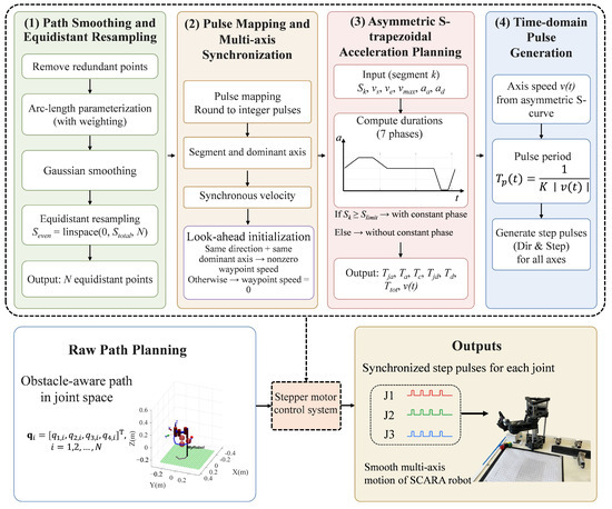
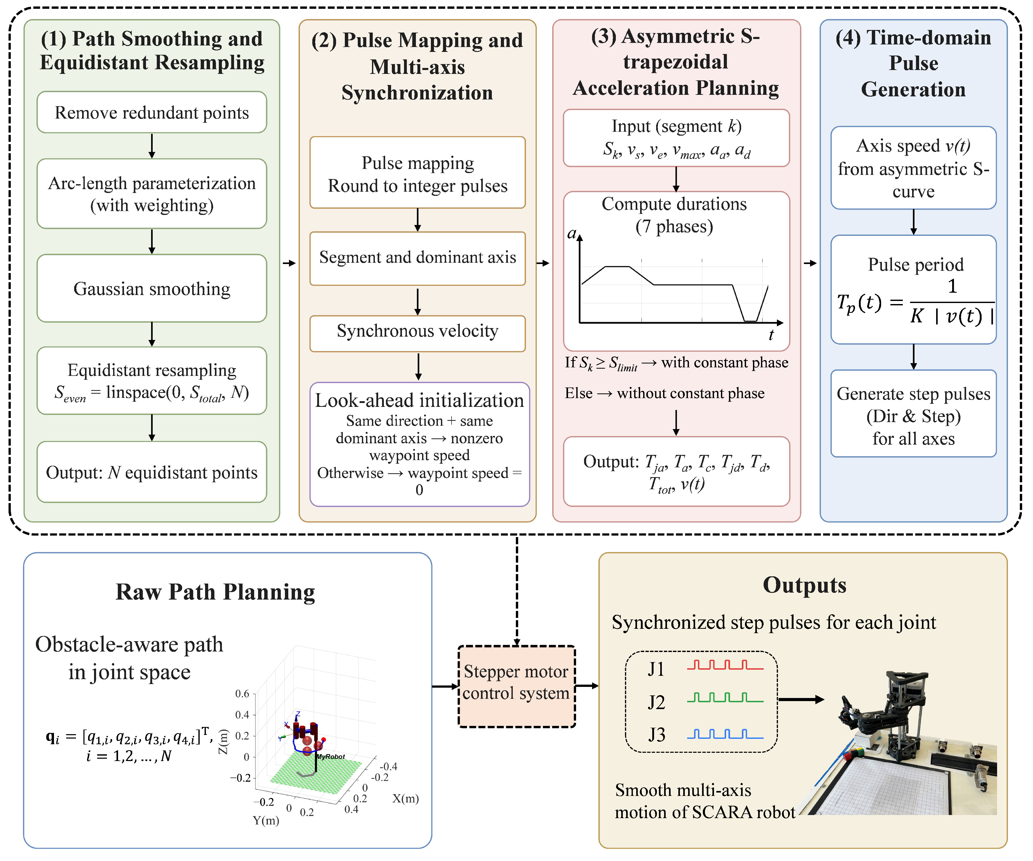
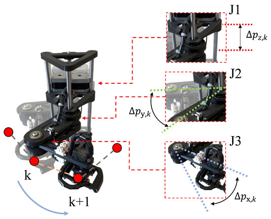
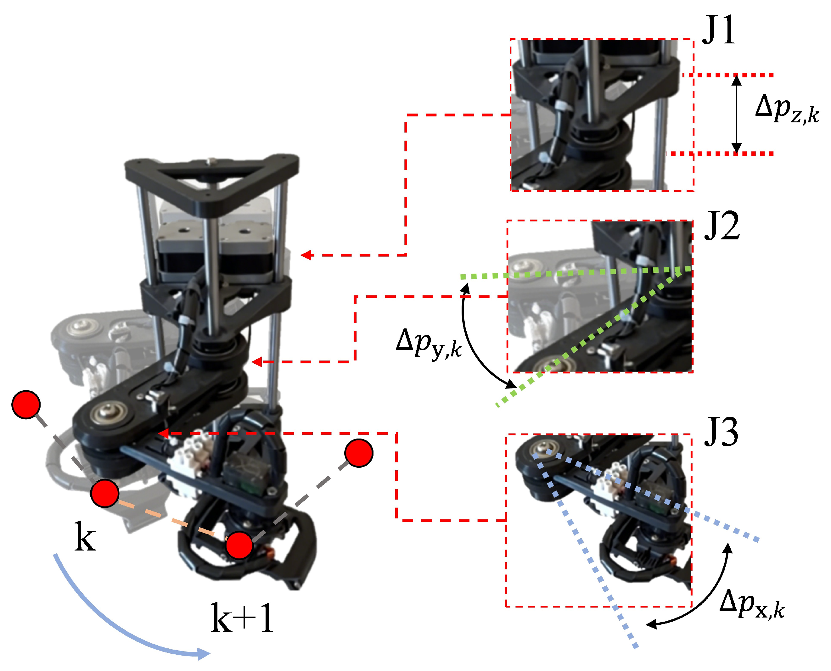
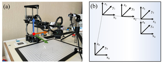
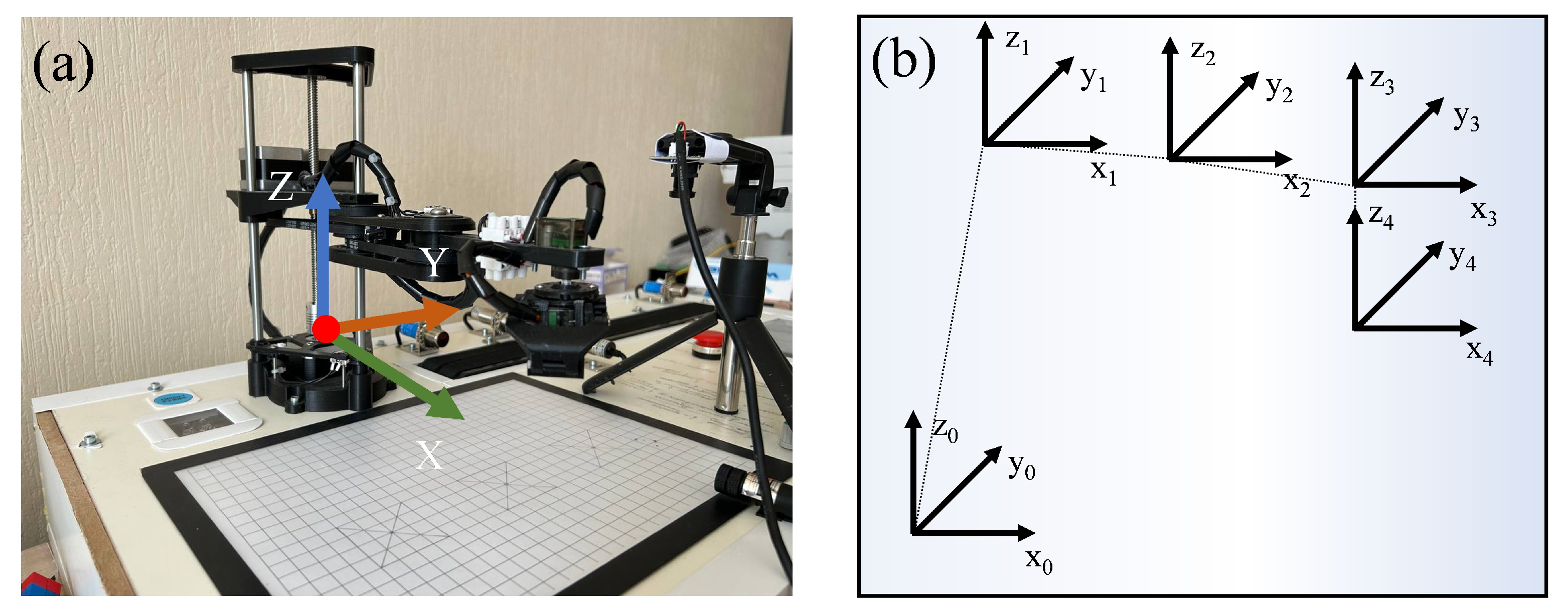
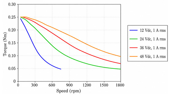
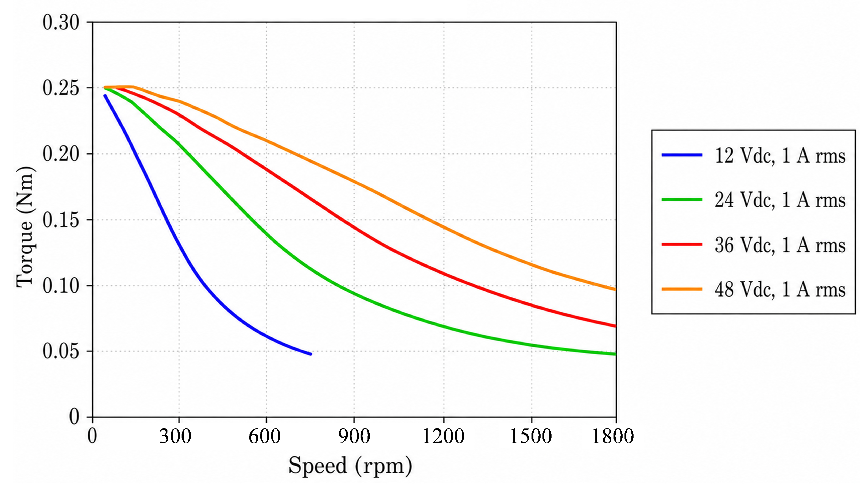
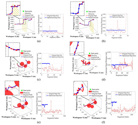
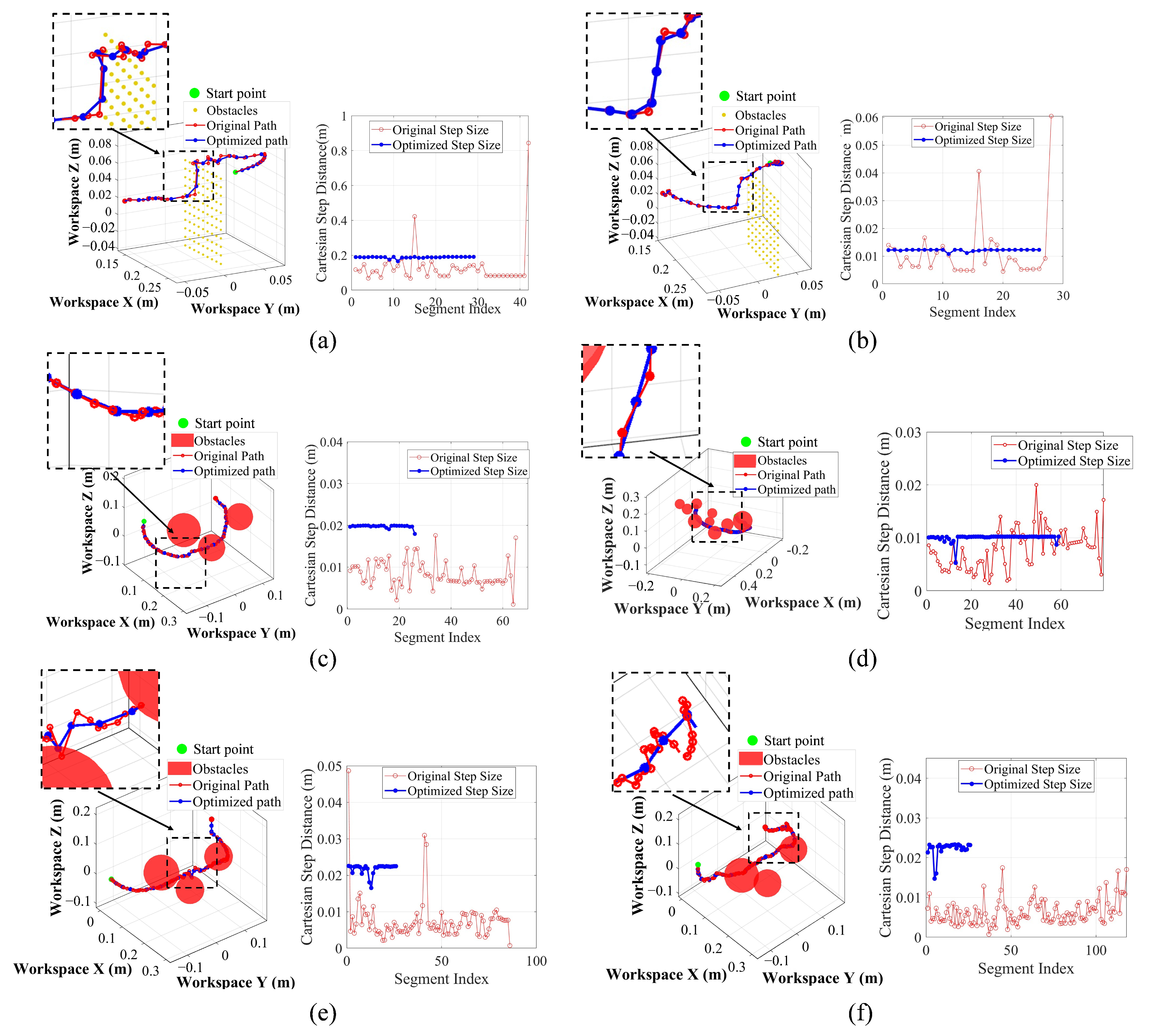
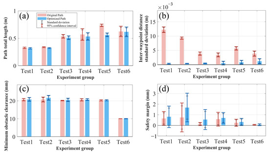
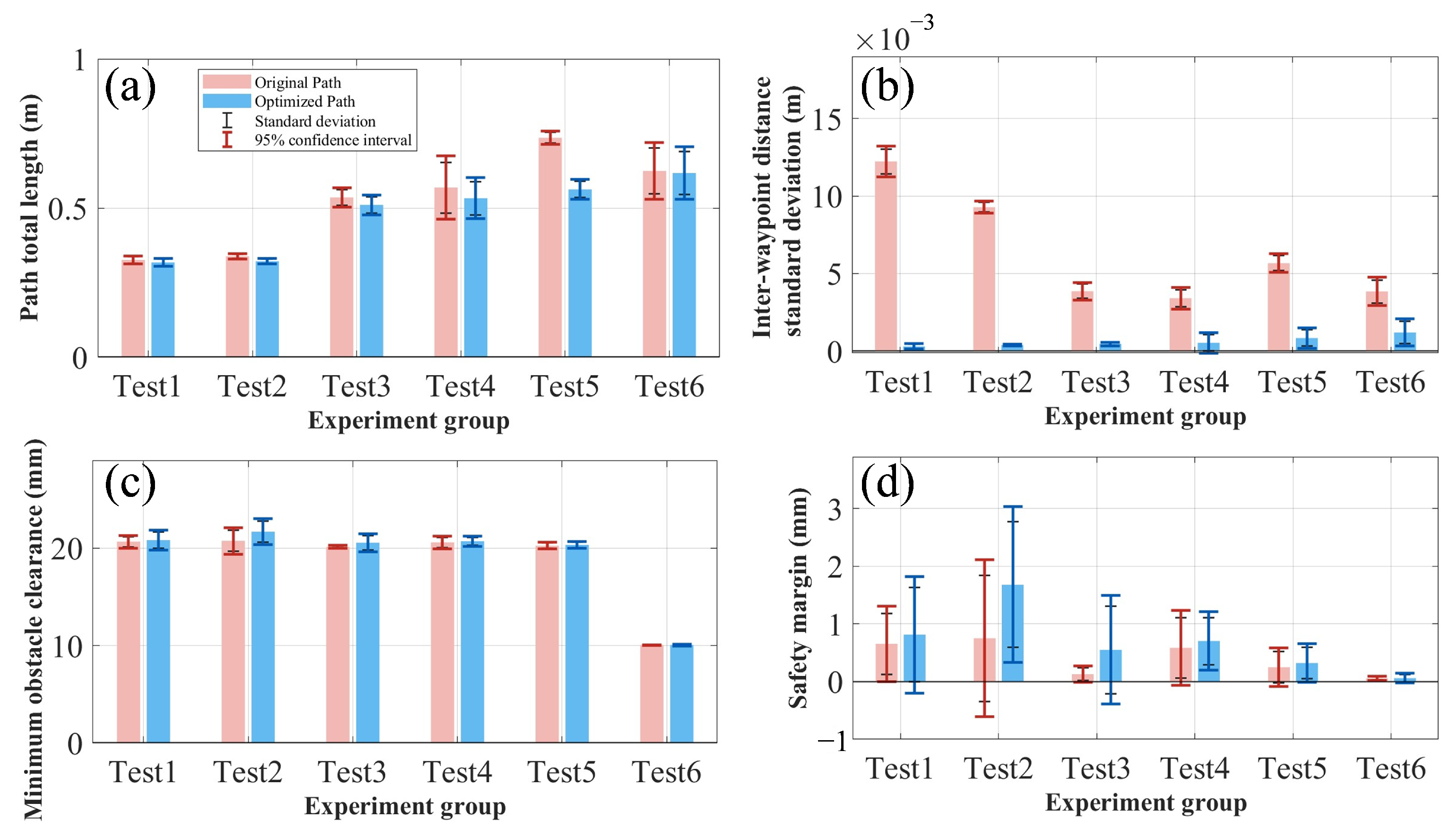
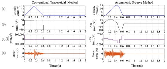
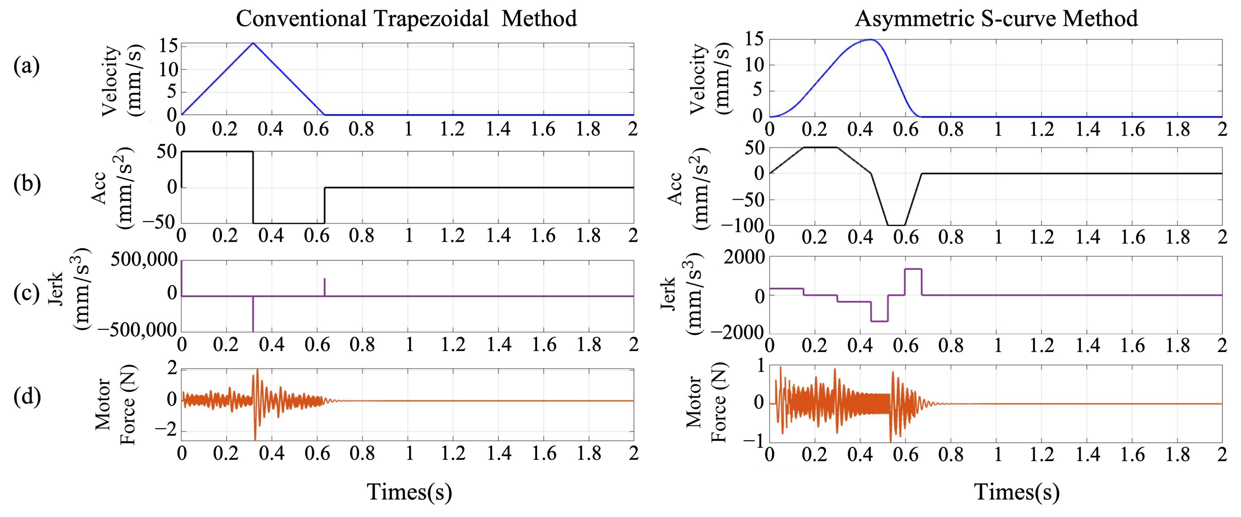
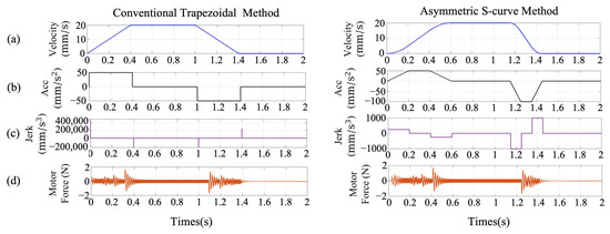
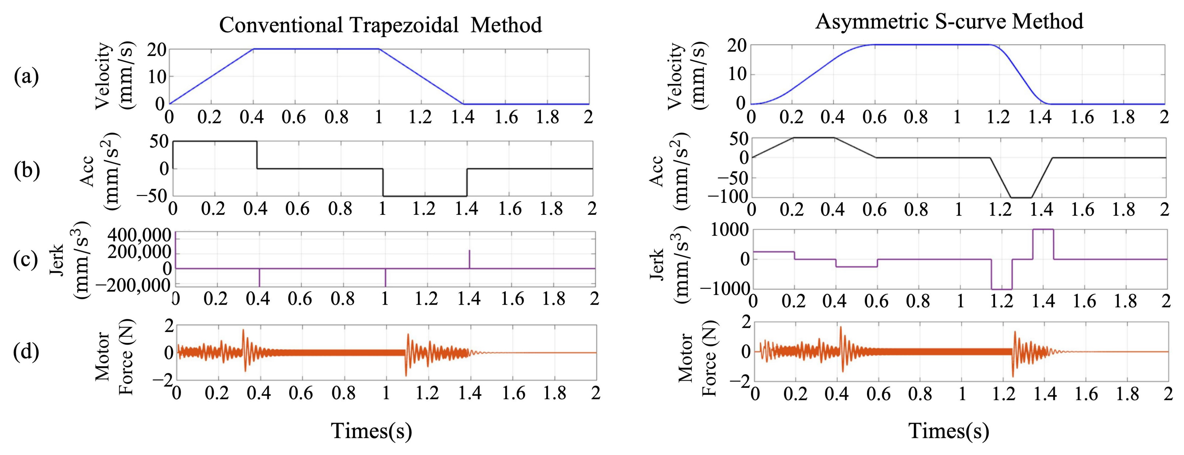
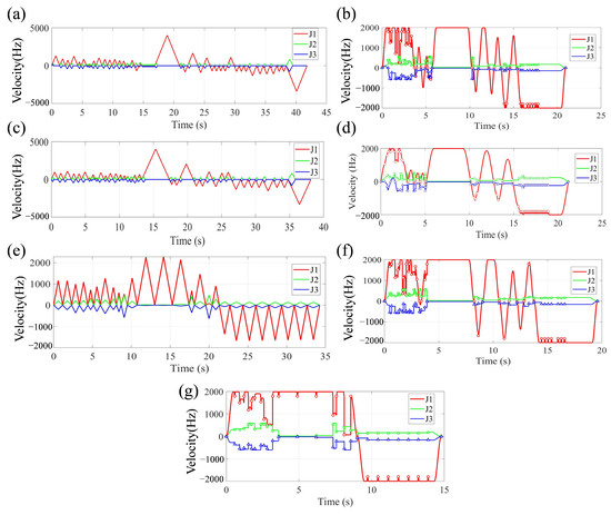
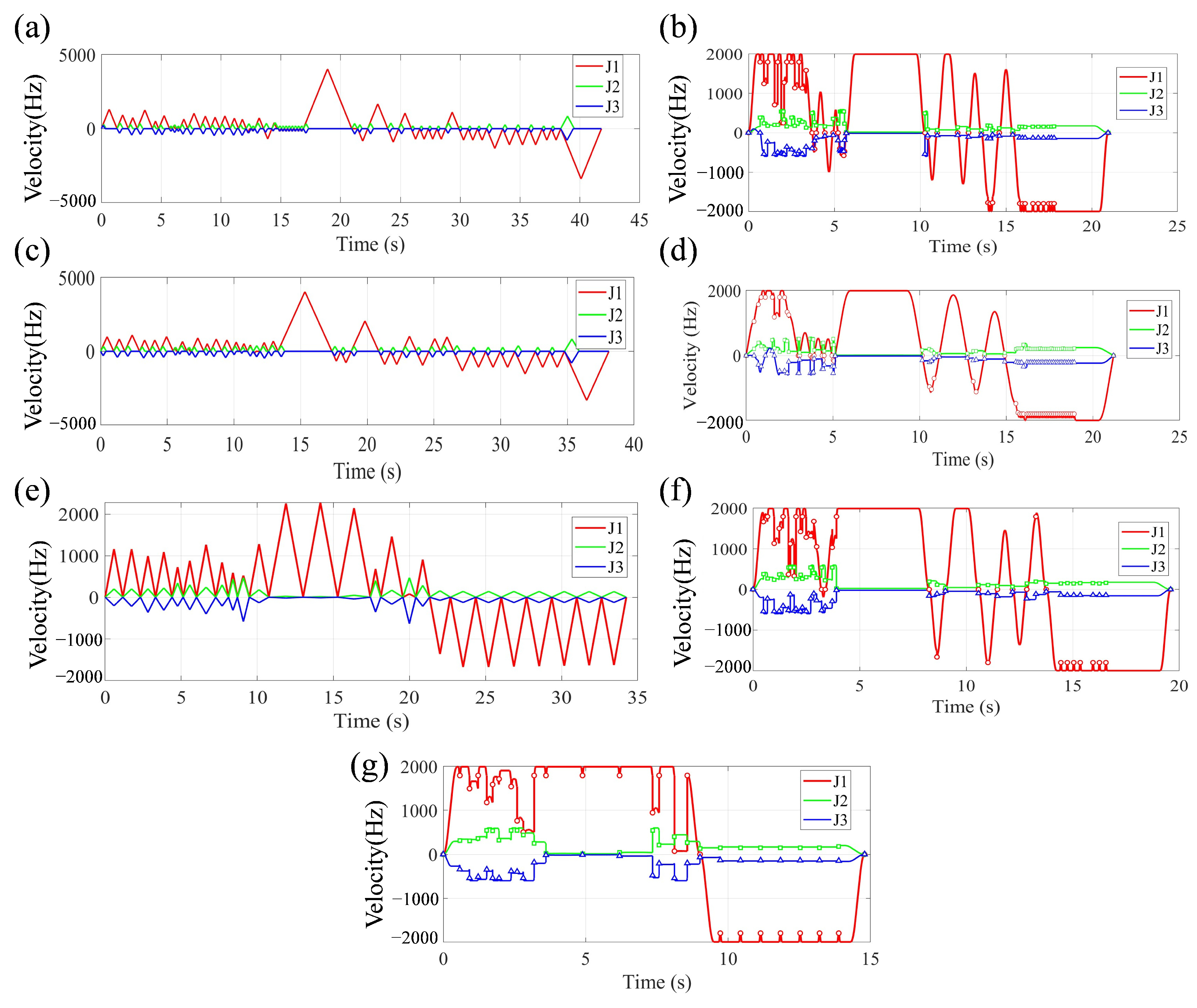
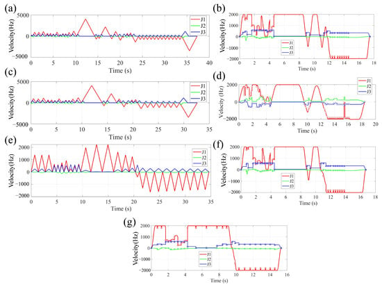
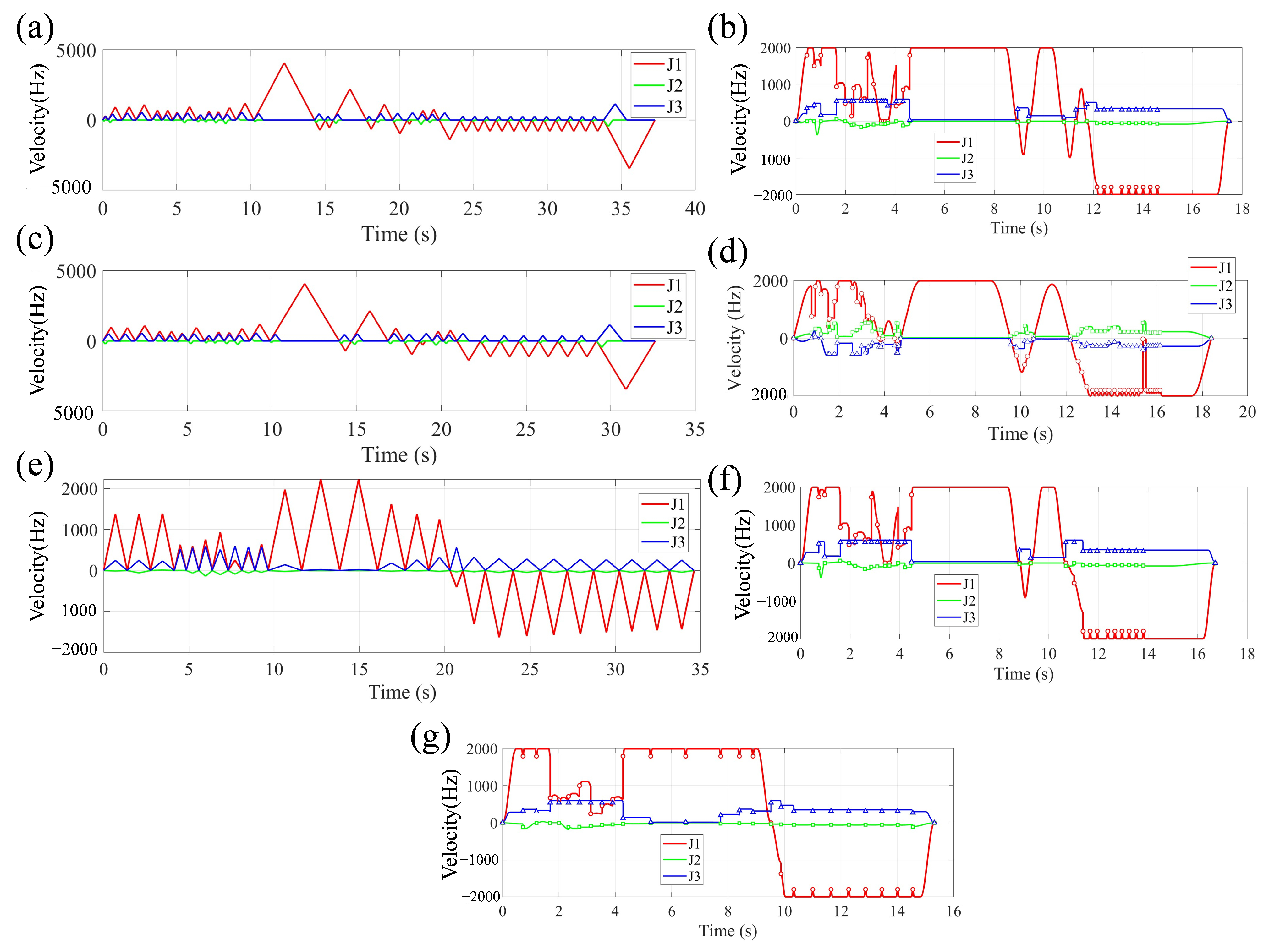
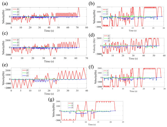
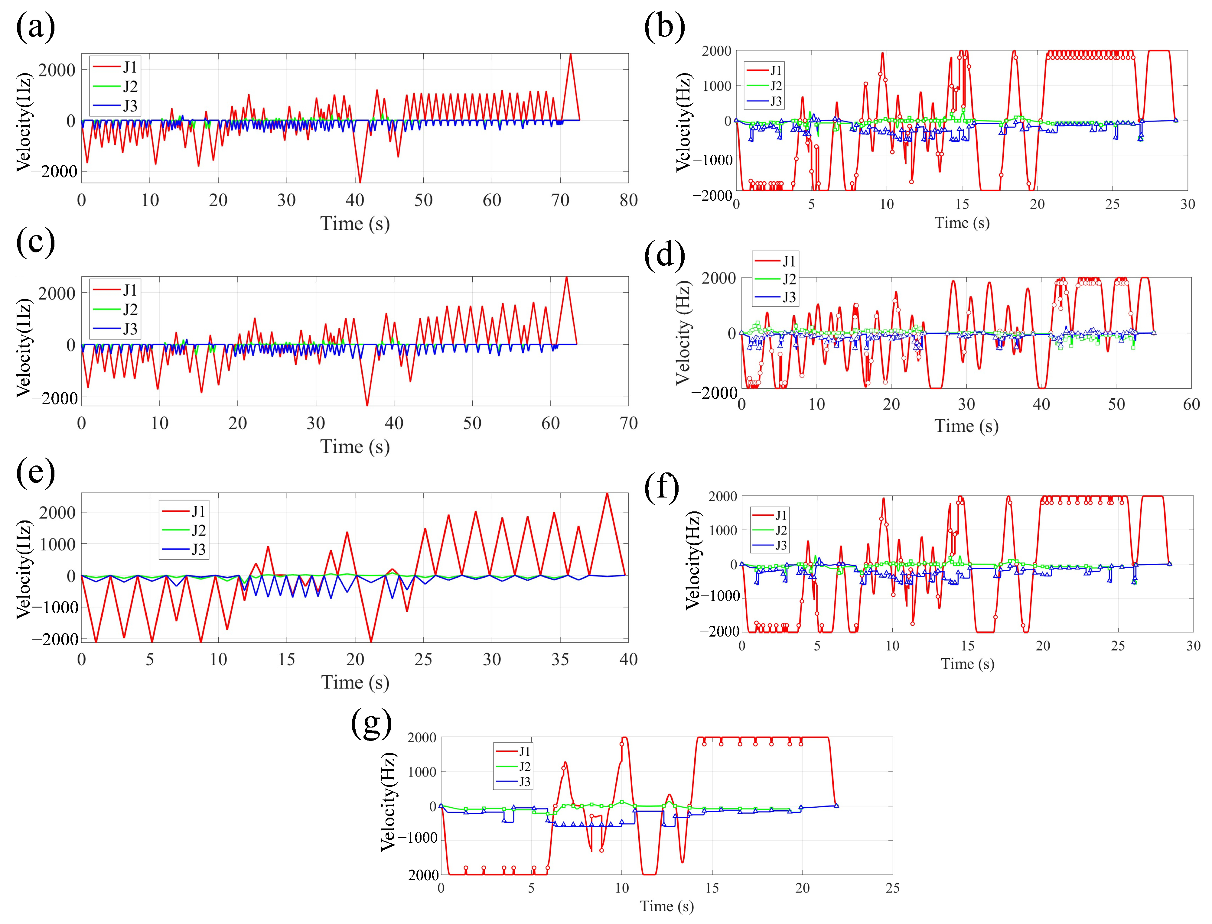
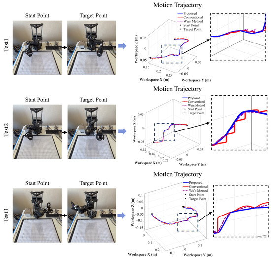
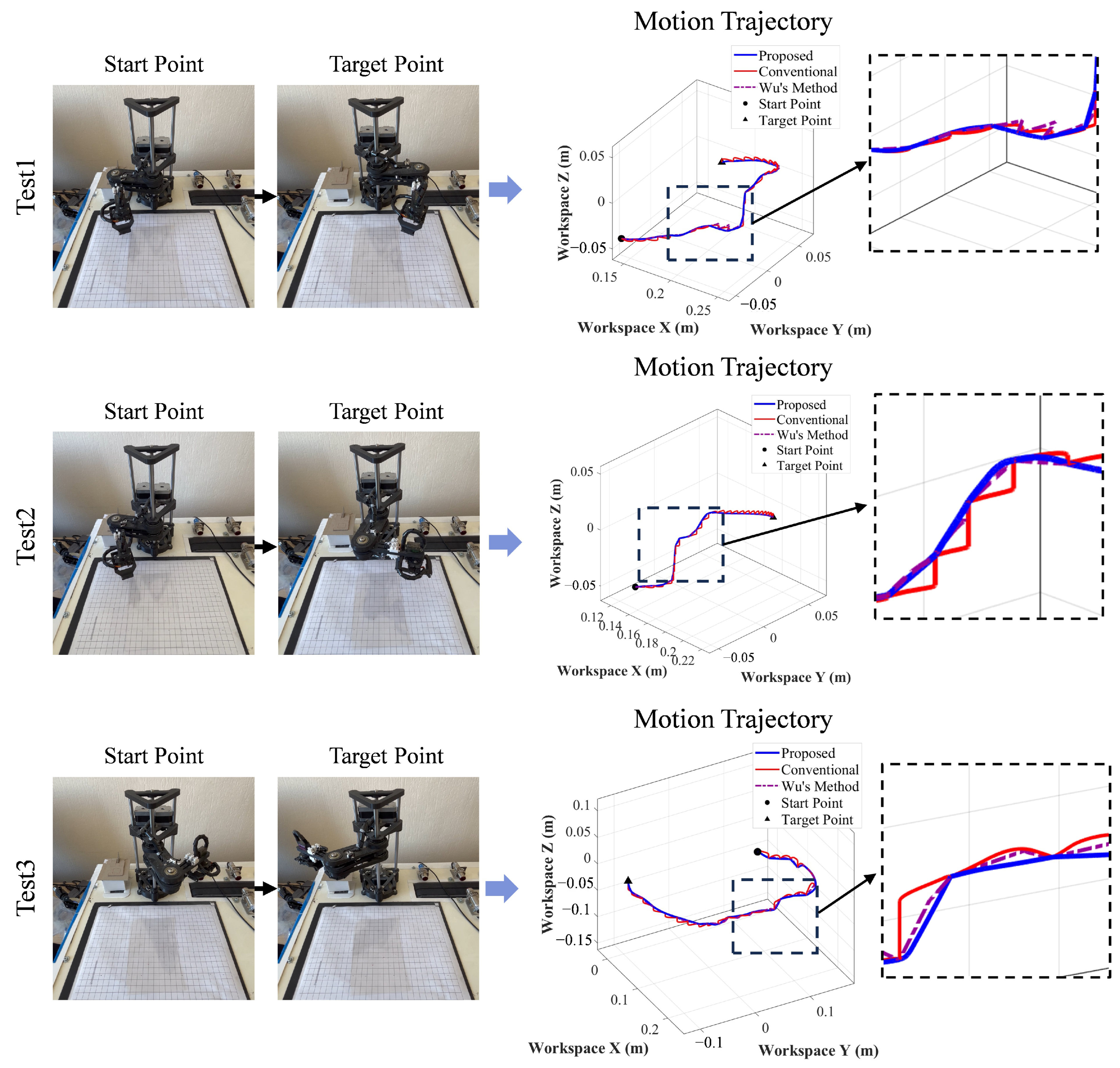
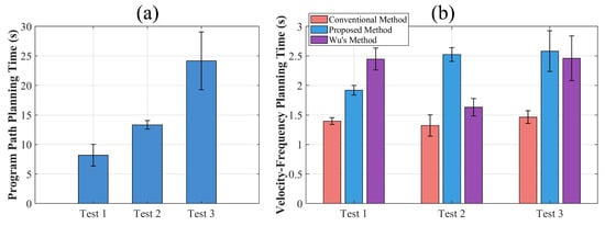
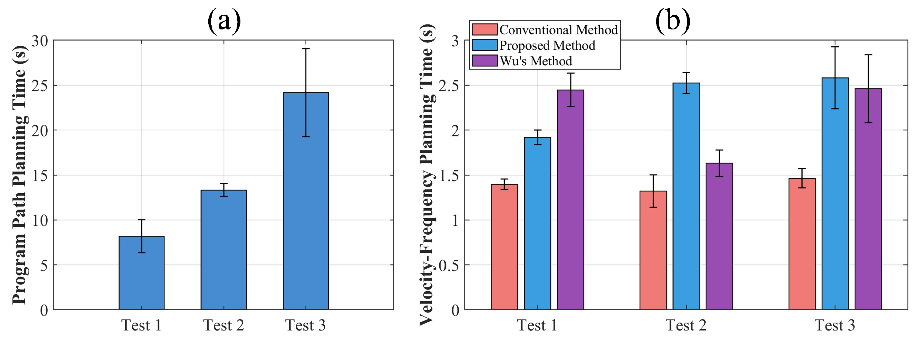
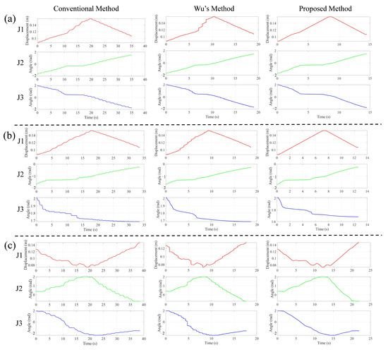
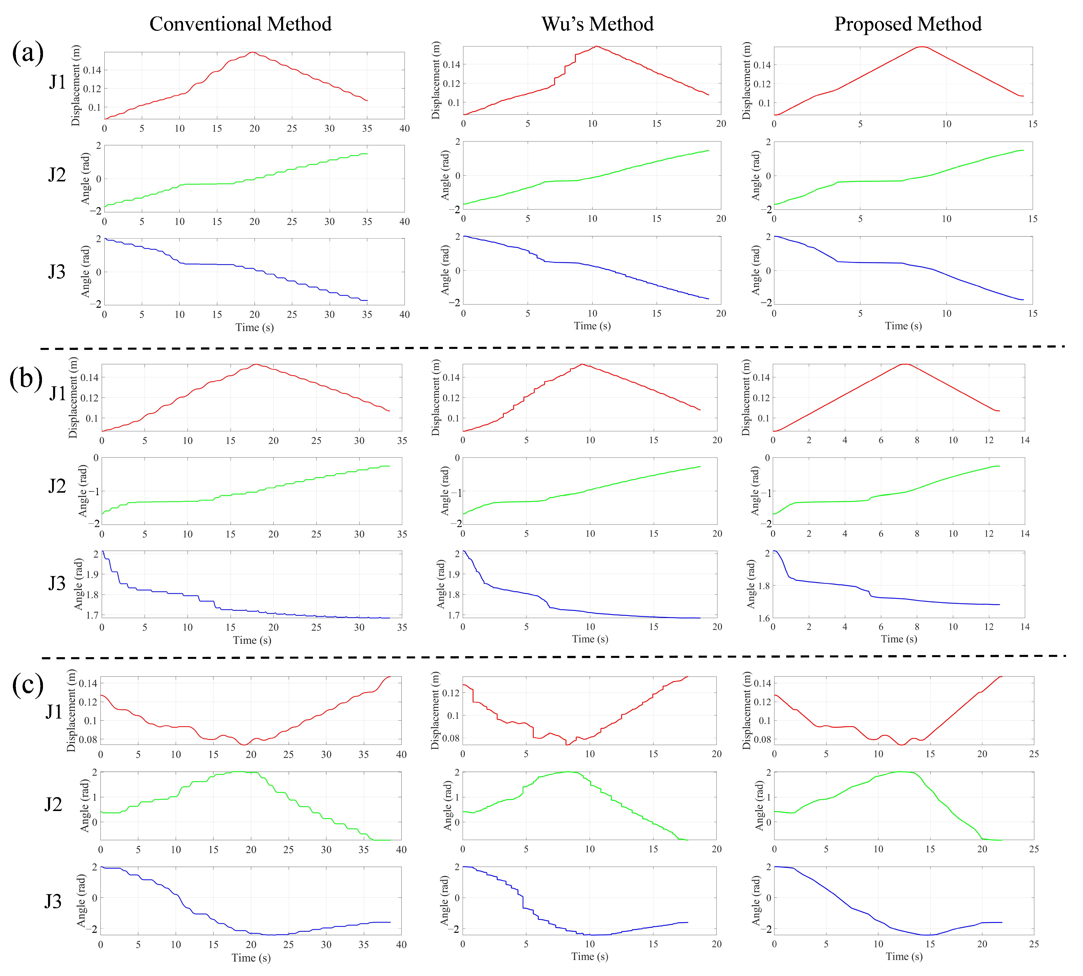
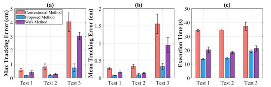
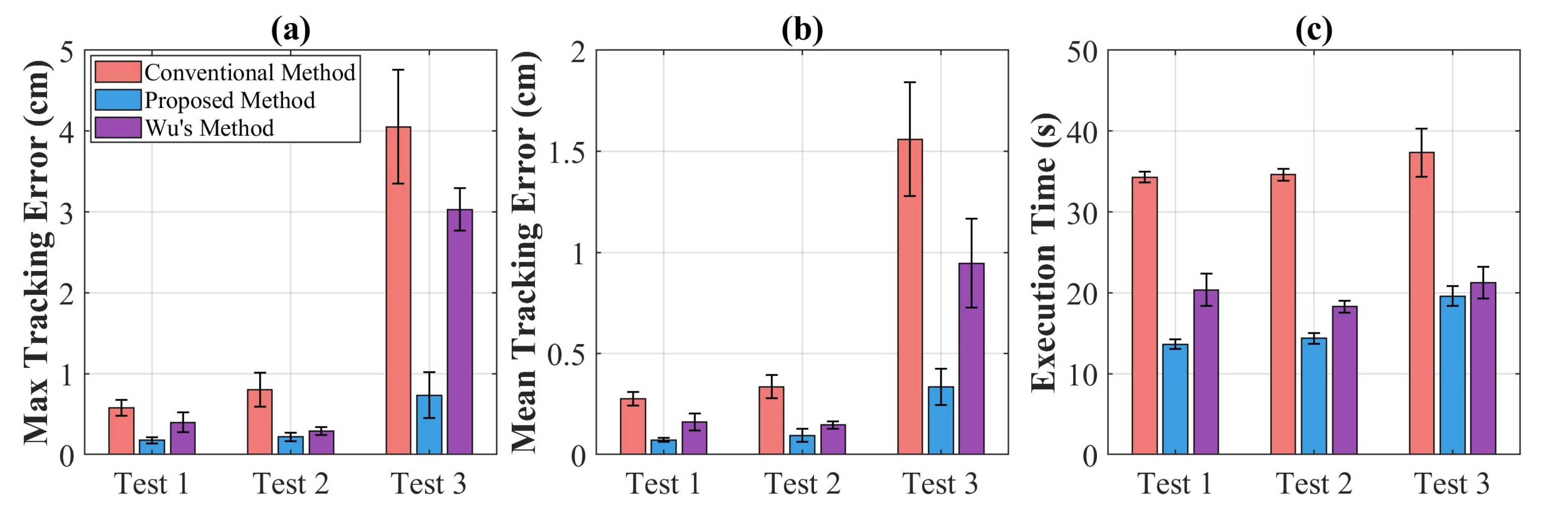

Disclaimer/Publisher’s Note: The statements, opinions and data contained in all publications are solely those of the individual author(s) and contributor(s) and not of MDPI and/or the editor(s). MDPI and/or the editor(s) disclaim responsibility for any injury to people or property resulting from any ideas, methods, instructions or products referred to in the content. |
© 2026 by the authors. Licensee MDPI, Basel, Switzerland. This article is an open access article distributed under the terms and conditions of the Creative Commons Attribution (CC BY) license.