Design and Motion Control Strategies for an Omniwheel System

Abstract

Space debris mitigation is a pivotal endeavor essential for sustaining human space exploration. To address the challenges posed by irregularly shaped, variably sized, and dynamically unpredictable debris in orbit, this paper proposes a mechanical design and motion control strategy for an omniwheel-based driving system. The mechanical architecture and kinematic principles of the system are elaborated in detail, complemented by the formulation of tailored motion control algorithms. First, the fundamental architecture of the driving subsystem is introduced, and the linear mapping between the uniformly distributed triad of omniwheels and the spherical drive is derived. Building upon this foundation, the kinematic transmission from the three evenly spaced driving subsystems to the contact sphere is established. This leads to the derivation of the overall linear mapping relationship between the nine uniformly distributed omniwheels and the contact sphere’s motion, thereby enabling precise trajectory tracking of the contact sphere via omniwheel actuation. Finally, comprehensive experimental validation was conducted in two phases. The first phase evaluated the fidelity and stability of the driving subsystem’s simulation model, as well as the accuracy of the kinematic mapping. Results demonstrate that the simulation model is highly stable and reliable. Under identical desired trajectories, the Root Mean Square Error (RMSE) between theoretical calculations and simulations was 4.082 × 10⁻⁴, while the RMSE between theory and physical prototypes was 0.0032. These results confirm that the motion errors remain within acceptable tolerances and the kinematic mapping is accurate. For the spherical end-effector, under the same trajectory conditions, the RMSE values among theoretical calculations, simulations, and physical prototypes were 0.0929 and 1.62, respectively. These findings validate the derived linear kinematic mapping, demonstrating its efficacy in precise motion control, which lays the foundation for future on-orbit detumbling tasks.

1. Introduction

The exploration of the vast cosmos serves as a driving force for global development, with the primary prerequisite for achieving this goal being the assurance of sustainable human space exploration [1,2,3]. However, as humanity’s activities in the space environment expand, space resources, particularly orbital resources, are becoming increasingly constrained. This scarcity is primarily attributed to two factors. First, the number of payloads in orbit has surged dramatically; the cataloged satellite population grew from 8892 in 2019 to an estimated 25,350 by 2026, representing a fourfold increase. Second, end-of-life payloads and spacecraft that have disintegrated due to mission failures cannot be autonomously removed from orbit. Over time, these defunct objects inevitably accumulate into space debris, with the currently tracked on-orbit debris population reaching 42,593. Consequently, there are two potential pathways to ensure the sustainable utilization of space resources: reducing the frequency of payload launches or actively removing existing space debris. Given that launch restrictions alone cannot fundamentally resolve this issue, Active Debris Removal (ADR) has emerged as a critical research direction.

From the perspectives of robotics and systems engineering, a complete ADR mission typically encompasses several sequential phases: launch, long-range rendezvous, close-proximity approach, capturing, and subsequent deorbiting. Extensive research on this technology has been conducted by various domestic and international institutions. Notable initiatives include:

• DEOS (Deutsche Orbital Servicing Mission) [4]: This mission is primarily designed for full-process on-orbit demonstration and validation. It aims to verify the entire control chain for safely approaching, grasping with an end-effector, detumbling, and deorbiting non-cooperative, tumbling satellites using a space robotic arm.
• EPOS (European Proximity Operations Simulator) [5]: Established by the German Aerospace Center (DLR), this Hardware-in-the-Loop (HIL) test facility utilizes two large industrial robots. It is specifically dedicated to simulating the contact dynamics involved when a robotic arm’s end-effector captures non-cooperative space debris.
• FREND (Front-End Robotics Enabling Near-Term Demonstration) [6]: This project focuses on developing a highly autonomous, high-stiffness robotic arm alongside specialized universal end-effectors. Its objective is to enable fully autonomous grasping and locking of non-cooperative satellites without human teleoperation from the ground.

Currently, prevalent ADR methodologies can be broadly classified into two categories. The first category comprises non-contact removal methods. These techniques alter the orbital trajectory of the debris—ultimately directing it into the atmosphere for disintegration—by remotely applying force fields or energy beams, thereby mitigating the risks associated with direct physical contact.

Existing research on non-contact methods includes the following approaches: (1) Gravitational Tractor: Lu and Love [7] proposed a concept that utilizes the spacecraft’s own mass to approach the debris, slowly “towing” it out of its original orbit through mutual gravitational attraction. In this scenario, the spacecraft hovers near the target (e.g., an asteroid or debris object) with its thrusters oriented outward, gradually deflecting the target from its trajectory. (2) Electrostatic Tether: Similarly, the electrostatic tug method employs Coulomb forces to deorbit space debris. The servicing spacecraft approaches the target debris and emits an electron beam toward it. The target accumulates excess electrons and becomes negatively charged, while the emitting tug acquires a positive charge. Consequently, the attractive force between these oppositely charged bodies is exploited to initiate the deorbiting process [8,9]. (3) Laser Ablation: Laser ablation is also recognized as an effective technique for space debris mitigation. This method involves irradiating the surface of the debris with high-energy lasers to induce localized vaporization and generate plasma plumes. The resulting reactive thrust alters the orbital trajectory of the debris. This approach primarily encompasses two configurations: Space-Based Lasers: Systems such as L’ADROIT utilize ultraviolet pulsed lasers, making them particularly suitable for removing small debris (<10 cm) that is difficult to capture using robotic arms. Ground-Based Lasers: Projects like LightForce employ continuous-wave lasers integrated with adaptive optics systems, which are primarily intended for immediate collision avoidance maneuvers [10,11,12,13,14,15,16,17].

The second category comprises contact-based removal methods, which can be further classified into rigid and flexible connections. Rigid connection methods require physical contact between the servicing spacecraft and the debris, typically achieved via robotic arms or grippers for locking. The primary approaches include: (1) Tentacle Capture: This method employs multiple flexible tentacles to grasp the debris from multiple points rather than relying on a single-point lock, as demonstrated in the ClearSpace-1 mission [18,19]. (2) Throwing Mechanism: This technique utilizes a rotating long arm to capture the debris. Centrifugal force is then used to fling the debris toward Earth’s atmosphere, while momentum exchange simultaneously propels the servicing spacecraft toward its next target [20,21,22,23]. (3) Adhesion-Based Capture: Inspired by bionics, this approach uses micro-patterned dry adhesives (MDAs) to adhere to debris in a vacuum environment [24,25,26]. (4) Docking: For satellites equipped with docking ports or specific geometric features, direct space docking can be performed. For instance, Astroscale’s ELSA-d mission utilizes magnetic or mechanical docking mechanisms to capture debris [26,27,28]. (5) Robotic Arm Capture: This method involves grasping debris using robotic arms and their end-effectors. Due to the rigid nature of the contact and the inherent tumbling motion of most space debris, pre-processing is generally required before engagement. Techniques include utilizing retractable flexible rods to make surface contact—synchronizing and slowing the debris rotation through friction and locking mechanisms or employing brushes to dissipate rotational kinetic energy via surface friction. Additionally, multi-arm systems are utilized where one arm performs the capture while another compensates for reaction forces to enhance stability. Furthermore, continuum manipulator arms, inspired by octopus tentacles or elephant trunks, offer infinite degrees of freedom, allowing superior adaptation to the complex shapes of non-cooperative targets [29,30,31,32,33,34,35].

Flexible connection methods primarily include: (1) Net Capturing [36,37,38,39]: The chaser satellite deploys a large net embedded with weighted blocks toward the debris using spring or pneumatic gun systems, enveloping the tumbling target. While nets permit a relatively safe standoff distance and exhibit high tolerance for unknown target geometries, controlling the tether dynamics of the resulting combined body is highly complex. (2) Harpoon Mechanisms [40,41]: This approach involves firing a barbed harpoon at high velocity to penetrate the shell structure of the debris, followed by towing it via a tether. (3) Tethered Robots/Tugs: These systems integrate tether technology with robotics. A representative example is the ROGER project, which uses a tether to connect to the target and tow it to a graveyard orbit [42,43].

Given that safety and reliability are paramount for on-orbit operations, capture methods involving rigid contact warrant further investigation. Existing research indicates that while robotic arm capture is a flexible and reliable approach, space debris typically exhibits complex motion and high angular velocities. Directly capturing such targets with a robotic arm risks collision; thus, pre-detumbling the target to reduce its angular velocity can significantly enhance the success rate of the capture operation. Current detumbling methodologies include: (1) Flexible Brush Detumbling [44]: This method involves mounting high-toughness, flexible brushes on the end-effector. As the robotic arm guides the effector against a non-cooperative target, continuous flexible micro-contacts and mechanical friction dissipate the target’s rotational kinetic energy as heat, thereby decaying single- or multi-axis spin rates. (2) Mechanical Impact/Push Detumbling [45]: This technique equips the end-effector with impact buffering mechanisms to perform multiple intermittent, active light touches or pushes against the tumbling target. Each impact absorbs energy through the buffer while applying a reverse impulsive torque, gradually halting the target through repeated micro-collisions. (3) Electromagnetic Eddy Current Detumbling: Since most space debris contains conductive materials like aluminum and titanium alloys, bringing electromagnetic coils from the servicing spacecraft near the rotating target induces eddy currents within the metallic shell. The relative motion generates an eddy current drag that exerts a non-contact detumbling torque on the target. (4) Electrostatic/Coulomb Force Detumbling: This approach utilizes onboard discharge devices to charge both the servicing spacecraft and the target with opposite polarities, thereby controlling the target’s attitude via Coulomb forces.

In contrast to the aforementioned non-contact and contact-based detumbling methods, this paper proposes a novel omniwheel-based active detumbling device. Unlike non-contact methods that rely on field-induced forces with limited control authority, and unlike contact-based methods such as flexible brush detumbling [44] and mechanical impact/push detumbling [45] that depend on passive energy dissipation through friction or intermittent contact, the proposed system achieves active, continuous, and precisely controllable rotational motion of a contact sphere through direct omniwheel actuation. By regulating the angular velocities of nine uniformly distributed omniwheels according to a derived closed-form kinematic mapping, the motion trajectory of the contact sphere can be commanded in real time, enabling adaptive detumbling strategies based on the target’s dynamic state. This represents a fundamental shift from passive energy dissipation to active motion control, directly addressing the low efficiency and lack of pronounced active capabilities inherent in existing approaches. To address this issue, this paper innovatively proposes a novel device that can be mounted on the end of a robotic arm to actively detumble the target. A critical analysis of existing detumbling methodologies reveals three principal limitations that motivate the proposed approach. First, non-contact methods exhibit low efficiency due to the rapid spatial decay of induced forces and the inability to generate sufficient torque for targets with high moments of inertia. Their control authority is fundamentally constrained by physical field propagation, precluding real-time adaptation to unpredictable target tumbling. Second, contact-based passive methods lack deterministic control: the detumbling rate depends on uncontrollable friction coefficients, surface roughness, and impact restitution, leading to highly variable outcomes and potential surface damage from repeated contact. Third, neither category provides trajectory-level motion control—existing methods cannot command a specific rotational trajectory for the target, which is essential for synchronized capture operations. The proposed omniwheel-based system directly addresses these limitations: (i) rigid rolling contact ensures deterministic force transmission without spatial decay; (ii) the closed-form kinematic model enables precise, real-time trajectory tracking of the contact sphere; (iii) motor-driven omniwheels provide active, modulated torque generation adaptable to target dynamics. The remainder of this paper is organized as follows: Section 2 introduces the structural composition and kinematic principles of the proposed detumbling device, deriving the kinematic transmission relationships and dynamics. Section 3 presents experimental validations, including comparative tests among theoretical derivations, simulation models, and physical prototypes, to verify the correctness of the derivations and lay the foundation for subsequent motion control. Section 4 provides a discussion of the results. Finally, Section 5 concludes the paper.

2. System Architecture and Kinematics

2.1. System Architecture

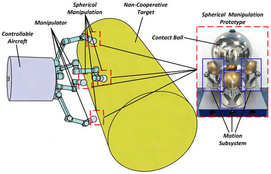
As illustrated in Figure 1, the on-orbit detumbling robotic system primarily consists of a controllable spacecraft, four robotic arms, a spherical end-effector mounted at the arm tips, and the space debris (hereafter uniformly referred to as non-cooperative targets throughout this paper). During operation in the space environment, the controllable spacecraft first approaches the non-cooperative target using its four robotic arms. Subsequently, the position and attitude of the spacecraft are stabilized while the robotic arms are actuated until the spherical end-effectors make contact with the target. Finally, the spherical end-effector is actively engaged to eliminate the target’s spin motion, after which the four robotic arms proceed with the capture task. The primary focus of this research lies on the spherical end-effector.

Figure 1. Composition of the detumbling robotic system.

As shown in Figure 1, the spherical end-effector primarily comprises a driving subsystem and a contact sphere. Three uniformly distributed driving subsystems maintain tight contact with the contact sphere without any relative slip. By actuating these driving subsystems, the motion of the contact sphere can be precisely controlled. The following section will first introduce the driving subsystem.

2.2. Driving Subsystem

2.2.1. Composition

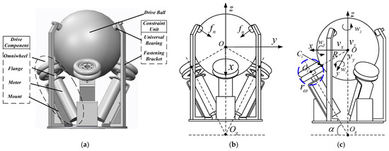
As illustrated in Figure 2a, the driving subsystem primarily consists of three components: a drive assembly, a driven sphere, and a constraint unit. The drive assembly is composed of four main parts: an omniwheel, a motor flange, a motor, and a motor bracket. Drum-shaped rollers are alternately mounted around the outer periphery of the omniwheel hub, allowing them to rotate freely and independently. The rotation of the hub provides the primary driving force, while the passive rotation of the rollers facilitates lateral sliding. This mechanism effectively reduces lateral friction and enhances overall motion efficiency. During operation, the motors actuate the three uniformly distributed omniwheels along their axes, thereby governing the motion of the driven sphere.

Figure 2. Driving subsystem: (a) 3D model; (b) Front-view schematic; (c) Side-view schematic.

The constraint unit mainly comprises universal bearings and fastening brackets. One end of the fastening bracket is mounted on the bottom connecting flange, while the other end supports the universal bearing. These bearings make gentle contact with the spherical end-effector, exerting a downward-inclined constraint force to prevent it from escaping during the detumbling process. Due to their low coefficient of friction, these bearings minimize energy dissipation caused by frictional resistance, ensuring that the driven sphere maintains its positional stability without deviation.

Figure 2b,c illustrate the geometric relationships of the driving subsystem. The geometric center of the driven sphere is defined as point $\mathit{O}$, which serves as the origin of the coordinate system. The X-axis is perpendicular to the current view and points outward; the Y-axis is parallel to the horizontal direction of the view, pointing to the right; and the Z-axis points vertically upward. The line connecting the universal bearing to point $\mathit{O}$ defines the direction of the pressing force ${\mathit{f}}_{\mathit{n}}$, which points towards $\mathit{O}$. Furthermore, the intersection point of the axes of the three omniwheels in the drive assembly is defined as ${\mathit{O}}_{\mathit{g}}$.

As shown in Figure 2c, the translational velocities of the driven sphere along the X, Y, and Z axes are denoted as ${\mathit{v}}_{\mathit{x}},{\mathit{v}}_{\mathit{y}},{\mathit{v}}_{\mathit{z}}$ respectively, while its angular velocities about these axes are denoted as ${\mathit{\omega }}_{\mathit{x}},{\mathit{\omega }}_{\mathit{y}},{\mathit{\omega }}_{\mathit{z}}$. The radius of the driven sphere is $\mathit{R}$. In terms of kinematics, the omniwheel can be modeled as an equivalent sphere, represented by the blue dashed lines in Fig. 2(c) with its center at ${\mathit{O}}_{\mathit{l}}$ and a radius of ${\mathit{r}}_{\mathit{w}}$. The contact points between the driven sphere and the equivalent spheres are denoted as ${\mathit{C}}_{\mathit{i}}\left(\mathit{i} = 1,2,3\right)$. Points $\mathit{O},{\mathit{O}}_{\mathit{l}},{\mathit{C}}_{\mathit{i}}$ are collinear. Additionally, the angle between the motor axis ${\mathit{O}}_{\mathit{l}}{\mathit{O}}_{\mathit{g}}$ and the horizontal plane is $\mathit{\alpha }$, and the line ${\mathit{O}}_{\mathit{l}}{\mathit{O}}_{\mathit{g}}$ is strictly perpendicular to the line $\mathit{O}{\mathit{O}}_{\mathit{l}}$.

2.2.2. Kinematic of the System

The translational velocity of the driving subsystem is defined as $\dot{\mathit{x} }\mathit{ϵ}{ \mathbf{R}}^{\mathbf{3}}$, and its angular velocity is denoted as $\dot{\mathbf{\Theta } }\mathbf{ϵ} {\mathbf{R}}^{\mathbf{3}}$, which are expressed in Equation (1) and Equation (2), respectively:

$$\dot{\mathit{x}} = {\left[\begin{array}{ccc}{\mathit{v}}_{\mathit{x}}& {\mathit{v}}_{\mathit{y}}& {\mathit{v}}_{\mathit{z}}\end{array}\right]}^{\mathit{T}}$$

(1)

$$\dot{\mathbf{\Theta }}={\left[\begin{array}{ccc}{\mathit{\omega }}_{\mathit{x}}& {\mathit{\omega }}_{\mathit{y}}& {\mathit{\omega }}_{\mathit{z}}\end{array}\right]}^{\mathit{T}}$$

(2)

where ${\mathit{v}}_{\mathit{x}},{\mathit{v}}_{\mathit{y}},{\mathit{v}}_{\mathit{z}}$ represent the translational velocities along the X, Y, and Z axes of the driven sphere’s coordinate system, respectively; ${\mathit{\omega }}_{\mathit{x}},{\mathit{\omega }}_{\mathit{y}},{\mathit{\omega }}_{\mathit{z}}$ denote the angular velocities about the corresponding axes.

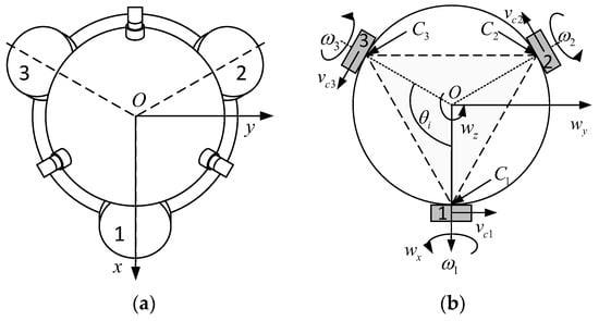
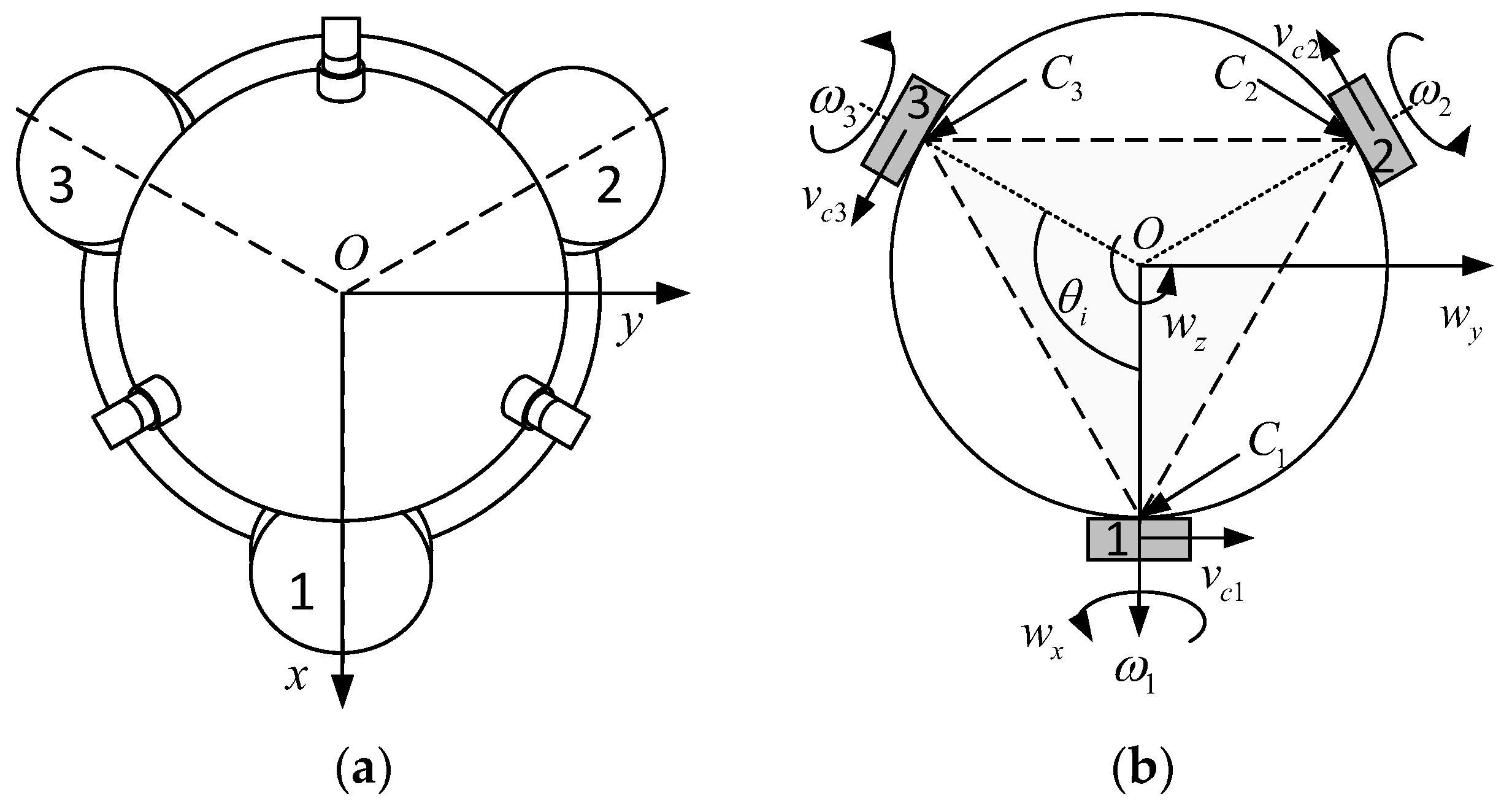
Figure 3a presents a top view of the driving subsystem, where the drive assemblies are sequentially numbered 1, 2, and 3 in a counterclockwise direction. Figure 3b illustrates the kinematic schematic. The angular velocities of omniwheels 1, 2, and 3 are defined as ${\mathit{\omega }}_1,{\mathit{\omega }}_2,{\mathit{\omega }}_3$, respectively, with their corresponding contact points on the driven sphere denoted as ${\mathit{C}}_1,{\mathit{C}}_2,{\mathit{C}}_3$. During motion, both the sphere and the omniwheels are assumed to be rigid bodies operating under a no-slip condition. Furthermore, the linear velocities generated by the omniwheels at the contact points ${\mathit{C}}_{\mathit{i}}\left(\mathit{i} = 1,2,3\right)$ are defined as ${\mathit{v}}_{\mathit{c}1},{\mathit{v}}_{\mathit{c}2},{\mathit{v}}_{\mathit{c}3}$. As shown in Figure 3b, the projections of the lines connecting the centers of omniwheels 1, 2, and 3 to the coordinate origin $\mathit{O}$ onto the XOY plane indicate that the omniwheels are uniformly distributed about the Z-axis of the driven sphere’s coordinate system, with an angular spacing of ${\mathit{\theta }}_{\mathit{i}}\left(\mathit{i} = 1,2,3\right)$.

Figure 3. Driving subsystem: (a) Top-view schematic; (b) Top-view kinematic diagram.

The angular velocities of the three omniwheels in the driving subsystem are defined as ${\mathit{\omega }}_{\mathit{o}}\mathbf{ϵ} {\mathbf{R}}^{\mathbf{3}}$, which is expressed in Equation (3):

$${\mathit{\omega }}_{\mathit{o}} = {\left[\begin{array}{ccc}{\mathit{\omega }}_1& {\mathit{\omega }}_2& {\mathit{\omega }}_3\end{array}\right]}^{\mathit{T}}$$

(3)

where ${\mathit{\omega }}_1,{\mathit{\omega }}_2,{\mathit{\omega }}_3$ represent the angular velocities of the omniwheels in drive assemblies 1, 2, and 3, respectively.

The position vector from the geometric center $\mathit{O}$ of the driven sphere to an arbitrary point on its surface is defined as ${\mathit{r}}_{\mathit{i}}^{\mathit{o}}\left(\mathit{i} = 1,2,3\right)$. Obviously, the magnitude satisfies $‖{\mathit{r}}_{\mathit{i}}^{\mathit{O}}‖ = \mathrm{R}$. Therefore, with respect to the coordinate frame at the sphere’s center $\mathit{O}$, the linear velocities ${\mathit{v}}_{\mathit{ci}}\left(\mathit{i} = 1,2,3\right)$ at the contact points ${\mathit{C}}_{\mathit{i}}\left(\mathit{i} = 1,2,3\right)$ are given by:

$${\mathit{v}}_{\mathit{ci}} = \dot{\mathit{x}} + \dot{\mathbf{\Theta } }\times {\mathit{r}}_{\mathit{i}}^{\mathit{o}}$$

(4)

For contact points ${\mathit{C}}_{\mathit{i}}\left(\mathit{i} = 1,2,3\right)$, the position vectors ${\mathit{r}}_{\mathit{i}}^{\mathit{o}}\left(\mathit{i} = 1,2,3\right)$ can be calculated using the spherical coordinate expression in Cartesian space, as given by Equation (5):

$${\mathit{r}}_{\mathit{i}}^{\mathit{o}} = \left[\begin{array}{c}\mathit{R}\cos \left({\mathit{\theta }}_{\mathit{i}}\right)\mathit{sin}\left(\mathsf{\pi }-\mathit{\alpha }\right)\\ \mathit{R}\sin \left({\mathit{\theta }}_{\mathit{i}}\right)\mathit{sin}\left(\mathsf{\pi }-\mathit{\alpha }\right)\\ \mathit{R}\cos \left(\mathsf{\pi }-\mathit{\alpha }\right)\end{array}\right]= \mathit{R}\left[\begin{array}{c}\cos \left({\mathit{\theta }}_{\mathit{i}}\right)\mathit{sin}\left(\mathit{\alpha }\right)\\ \sin \left({\mathit{\theta }}_{\mathit{i}}\right)\mathit{sin}\left(\mathit{\alpha }\right)\\ -\cos \left(\mathit{\alpha }\right)\end{array}\right]$$

(5)

where ${\mathit{\theta }}_{\mathit{i}}$ represents the uniform distribution angle of the omniwheels, corresponding to the elevation angle in the spherical coordinate system; and $\mathit{\alpha }$ denotes the angle between the omniwheel axis and the horizontal plane, corresponding to the azimuth angle.

The cross product of vectors in three-dimensional space is calculated as given by Equation (6):

$$\mathit{a} \times \mathit{b} =\left[\begin{array}{ccc}\mathit{i}& \mathit{j}& \mathit{k}\\ {\mathit{x}}_1& {\mathit{y}}_1& {\mathit{z}}_1\\ {\mathit{x}}_2& {\mathit{y}}_2& {\mathit{z}}_2\end{array}\right] =\begin{array}{c}\left({\mathit{y}}_1{\mathit{z}}_2-{\mathit{y}}_2{\mathit{z}}_1\right)\mathit{i}\\ \left({\mathit{x}}_1{\mathit{z}}_2-{\mathit{x}}_2{\mathit{z}}_1\right)\mathit{j}\\ \left({\mathit{x}}_1{\mathit{y}}_2-{\mathit{x}}_2{\mathit{y}}_1\right)\mathit{k}\end{array}$$

(6)

where $\mathit{a} = \left({\mathrm{x}}_1,{\mathrm{y}}_1,{\mathrm{z}}_1\right)$, $\mathit{b} = \left({\mathrm{x}}_2,{\mathrm{y}}_2,{\mathrm{z}}_2\right)$.

Combining the above equations yields Equation (7):

$$\dot{\mathbf{\Theta }} \times {\mathit{r}}_{\mathit{i}}^{\mathit{o}} = \mathit{R}\left[\begin{array}{l}-{\mathit{\omega }}_{\mathit{y}}\mathit{cos}\mathit{\alpha }-{\mathit{\omega }}_{\mathit{z}}\mathit{sin}\left({\mathit{\theta }}_{\mathit{i}}\right)\mathit{sin}\mathit{\alpha }\\ {\mathit{\omega }}_{\mathit{z}}\mathit{cos}\left({\mathit{\theta }}_{\mathit{i}}\right)\mathit{sin}\mathit{\alpha } + {\mathit{\omega }}_{\mathit{x}}\mathit{cos}\mathit{\alpha }\\ \mathit{sin}\mathit{\alpha }({\mathit{\omega }}_{\mathit{x}}\mathit{sin}\left({\mathit{\theta }}_{\mathit{i}}\right)-{\mathit{\omega }}_{\mathit{y}}\mathit{cos}\left({\mathit{\theta }}_{\mathit{i}}\right))\end{array}\right]$$

(7)

Combining Equations (6) and (7) yields the linear velocities ${\mathit{v}}_{\mathit{ci}}\left(\mathit{i} = 1,2,3\right)$ at the contact points ${\mathit{C}}_{\mathit{i}}\left(\mathit{i} = 1,2,3\right)$, with respect to the coordinate frame at the sphere’s center $\mathit{O}$:

$${\mathit{v}}_{\mathit{ci}} =\left[\begin{array}{c}{\mathit{v}}_{\mathit{x}}\\ {\mathit{v}}_{\mathit{y}}\\ {\mathit{v}}_{\mathit{z}}\end{array}\right]+ \mathit{R}\left[\begin{array}{l}-{\mathit{\omega }}_{\mathit{y}}\mathit{cos}\mathit{\alpha }-{\mathit{\omega }}_{\mathit{z}}\mathit{sin}\left({\mathit{\theta }}_{\mathit{i}}\right)\mathit{sin}\mathit{\alpha }\\ {\mathit{\omega }}_{\mathit{z}}\mathit{cos}\left({\mathit{\theta }}_{\mathit{i}}\right)\mathit{sin}\mathit{\alpha } + {\mathit{\omega }}_{\mathit{x}}\mathit{cos}\mathit{\alpha }\\ \mathit{sin}\mathit{\alpha }({\mathit{\omega }}_{\mathit{x}}\mathit{sin}\left({\mathit{\theta }}_{\mathit{i}}\right)-{\mathit{\omega }}_{\mathit{y}}\mathit{cos}\left({\mathit{\theta }}_{\mathit{i}}\right))\end{array}\right]=\left[\begin{array}{l}{\mathit{v}}_{\mathit{x}}-\mathit{R}({\mathit{\omega }}_{\mathit{y}}\mathit{cos}\mathit{\alpha } +{ \mathit{\omega }}_{\mathit{z}}\mathit{sin}\left({\mathit{\theta }}_{\mathit{i}}\right)\mathit{sin}\mathit{\alpha })\\ {\mathit{v}}_{\mathit{y}}+\mathit{R}({\mathit{\omega }}_{\mathit{z}}\mathit{cos}\left({\mathit{\theta }}_{\mathit{i}}\right)\mathit{sin}\mathit{\alpha } +{ \mathit{\omega }}_{\mathit{x}}\mathit{cos}\mathit{\alpha })\\ {\mathit{v}}_{\mathit{z}}+\mathit{R}(\mathit{sin}\mathit{\alpha }({\mathit{\omega }}_{\mathit{x}}\mathit{sin}\left({\mathit{\theta }}_{\mathit{i}}\right)-{\mathit{\omega }}_{\mathit{y}}\mathit{cos}\left({\mathit{\theta }}_{\mathit{i}}\right)))\end{array}\right]$$

(8)

The direction vector ${\mathit{t}}_{\mathit{i}}^{\mathit{o}} \mathbf{ϵ}{ \mathbf{R}}^{\mathbf{3}}\left(i = 1,2,3\right)$ from the omniwheel i to the contact point ${\mathit{C}}_{\mathit{i}}\left(\mathit{i} = 1,2,3\right)$ is defined as:

$${\mathit{t}}_{\mathit{i}}^{\mathit{o}} = \left[\begin{array}{l}-\mathit{sin}\left({\mathit{\theta }}_{\mathit{i}}\right)\\ \mathit{cos}\left({\mathit{\theta }}_{\mathit{i}}\right)\\ 0\end{array}\right]$$

(9)

Since the points $\mathit{O},{\mathit{O}}_{\mathit{l}},{\mathit{C}}_{\mathit{i}}$ are collinear, the following geometric relationship holds, as given by Equation (10):

$${{\mathit{t}}_{\mathit{i}}^{\mathit{o}}}^{\mathrm{T}}{\mathit{r}}_{\mathit{i}}^{\mathit{o}} = 0$$

(10)

where ${{\mathit{t}}_{\mathit{i}}^{\mathit{o}}}^{\mathrm{T}}$ denotes the transpose of matrix ${\mathrm{t}}_{\mathrm{i}}^{\mathrm{o}}$.

During the motion, the omniwheels maintain rolling contact with the rigid sphere without relative slipping. Based on the non-slipping constraint equations, it can be readily obtained that:

$${{\mathit{t}}_{\mathit{i}}^{\mathit{o}}}^{\mathrm{T}}\times {\mathit{v}}_{\mathit{ci}} = r_{\mathit{\omega }}{\mathit{\omega }}_{\mathit{o}}$$

(11)

Further, we can obtain:

$${{\mathit{t}}_{\mathit{i}}^{\mathit{o}}}^{\mathrm{T}}\times {\mathit{v}}_{\mathit{ci}} = {{\mathit{t}}_{\mathit{i}}^{\mathit{o}}}^{\mathrm{T}}(\dot{\mathit{x}} +\dot{ \mathbf{\Theta }} \times {\mathit{r}}_{\mathit{i}}^{\mathit{o}}) = {{\mathit{t}}_{\mathit{i}}^{\mathit{o}}}^{\mathrm{T}}\dot{\mathit{x}} + {{\mathit{t}}_{\mathit{i}}^{\mathit{o}}}^{\mathrm{T}}(\dot{\mathbf{\Theta } }\times { \mathit{r}}_{\mathit{i}}^{\mathit{o}})$$

(12)

$${{\mathit{t}}_{\mathit{i}}^{\mathit{o}}}^{\mathrm{T}}\dot{\mathit{x}}=\left[\begin{array}{ccc}-\mathit{sin}\left({\mathit{\theta }}_{\mathit{i}}\right)& \mathit{cos}\left({\mathit{\theta }}_{\mathit{i}}\right)& 0\end{array}\right]\left[\begin{array}{c}{\mathit{v}}_{\mathit{x}}\\ {\mathit{v}}_{\mathit{y}}\\ {\mathit{v}}_{\mathit{z}}\end{array}\right]=-\mathit{sin}\left({\mathit{\theta }}_{\mathit{i}}\right){\mathit{v}}_{\mathit{x} }+\mathit{cos}\left({\mathit{\theta }}_{\mathit{i}}\right){\mathit{v}}_{\mathit{y}}$$

(13)

$${{\mathit{t}}_{\mathit{i}}^{\mathit{o}}}^{\mathrm{T}}(\dot{\mathbf{\Theta }} \times {\mathit{r}}_{\mathit{i}}^{\mathit{o}})=\mathit{R}({\mathit{\omega }}_{\mathit{y}}\mathit{sin}\left({\mathit{\theta }}_{\mathit{i}}\right)\mathit{cos}\mathit{\alpha }+{ \mathit{\omega }}_{\mathit{z}}\mathit{sin}\mathit{\alpha }+{\mathit{\omega }}_{\mathit{x}}\mathit{cos}\left({\mathit{\theta }}_{\mathit{i}}\right)\mathit{cos}\mathit{\alpha })$$

(14)

Combining Equations (11) and (14):

$${\mathit{\omega }}_{\mathit{i}}={\displaystyle \frac{-\mathit{sin}\left({\mathit{\theta }}_{\mathit{i}}\right){\mathit{v}}_{\mathit{x}} + \mathit{cos}\left({\mathit{\theta }}_{\mathit{i}}\right){\mathit{v}}_{\mathit{y}} + \mathit{R}({\mathit{\omega }}_{\mathit{y}}\mathit{sin}\left({\mathit{\theta }}_{\mathit{i}}\right)\mathit{cos}\mathit{\alpha } +{ \mathit{\omega }}_{\mathit{z}}\mathit{sin}\mathit{\alpha } +{ \mathit{\omega }}_{\mathit{x}}\mathit{cos}\left({\mathit{\theta }}_{\mathit{i}}\right)\mathit{cos}\mathit{\alpha })}{{\mathit{r}}_{\mathit{\omega }}}}$$

(15)

Due to the structural characteristics of the driving subsystem, the driven sphere does not undergo translational motion under the constraint unit, satisfying the relationships given by Equations (16) and (17):

$${\mathit{v}}_{\mathit{x}} \equiv 0$$

(16)

$${\mathit{v}}_{\mathit{y}} \equiv 0$$

(17)

Equation (15) can then be further simplified into Equation (18):

$${\mathit{\omega }}_{\mathit{o}} = {\displaystyle \frac{\mathit{R}({\mathit{\omega }}_{\mathit{y}}\mathit{sin}\left({\mathit{\theta }}_{\mathit{i}}\right)\mathit{cos}\mathit{\alpha } + {\mathit{\omega }}_{\mathit{z}}\mathit{sin}\mathit{\alpha } + {\mathit{\omega }}_{\mathit{x}}\mathit{cos}\left({\mathit{\theta }}_{\mathit{i}}\right)\mathit{cos}\mathit{\alpha })}{{\mathit{r}}_{\mathit{\omega }}}}$$

(18)

Equation (18) can be further rearranged as Equation (19):

$$\dot{\mathbf{\Theta } }= {\displaystyle \frac{{\mathit{r}}_{\mathit{\omega }}}{\mathit{R}}}{\left({\mathit{B}\left({\mathit{\theta }}_{\mathit{i}},\mathit{\alpha }\right)}^{\mathit{T}}\mathit{B}\left({\mathit{\theta }}_{\mathit{i}},\mathit{\alpha }\right)\right)}^{-1}{\mathit{B}\left({\mathit{\theta }}_{\mathit{i}},\mathit{\alpha }\right)}^{\mathit{T}}\mathit{\omega } = {\displaystyle \frac{\mathit{R}}{{\mathit{r}}_{\mathit{\omega }}}}\mathit{B}\left({\mathit{\theta }}_{\mathit{i}},\mathit{\alpha }\right)\dot{\mathbf{\Theta }}\left(\mathit{i} = 1,2,3\right)$$

(19)

where $\mathit{B}\left({\mathit{\theta }}_{\mathit{i}},\mathit{\alpha }\right) = \left[\begin{array}{ccc}\mathit{cos}\left({\mathit{\theta }}_1\right)\mathit{cos}\mathit{\alpha }& \mathit{sin}\left({\mathit{\theta }}_1\right)\mathit{cos}\mathit{\alpha }& \mathit{sin}\mathit{\alpha }\\ \mathit{cos}\left({\mathit{\theta }}_2\right)\mathit{cos}\mathit{\alpha }& \mathit{sin}\left({\mathit{\theta }}_2\right)\mathit{cos}\mathit{\alpha }& \mathit{sin}\mathit{\alpha }\\ \mathit{cos}\left({\mathit{\theta }}_3\right)\mathit{cos}\mathit{\alpha }& \mathit{sin}\left({\mathit{\theta }}_3\right)\mathit{cos}\mathit{\alpha }& \mathit{sin}\mathit{\alpha }\end{array}\right]$, ${\mathit{\omega }}_{\mathit{o}} = \left[\begin{array}{c}{\mathit{\omega }}_1\\ {\mathit{\omega }}_2\\ {\mathit{\omega }}_3\end{array}\right]$, $\dot{\mathbf{\Theta } }= \left[\begin{array}{c}{\mathit{\omega }}_{\mathit{x}}\\ {\mathit{\omega }}_{\mathit{y}}\\ {\mathit{\omega }}_{\mathit{z}}\end{array}\right]$.

Equation (19) fully illustrates the mapping relationship from the motion of the driven sphere to that of each omniwheel. Since the actual operation involves the inverse process of this mapping, the Moore–Penrose method is employed to invert Equation (19), yielding Equation (20):

$$\dot{\mathbf{\Theta } }= {\displaystyle \frac{{\mathit{r}}_{\mathit{\omega }}}{\mathit{R}}}{\left({\mathit{B}\left({\mathit{\theta }}_{\mathit{i}},\mathit{\alpha }\right)}^{\mathit{T}}\mathit{B}\left({\mathit{\theta }}_{\mathit{i}},\mathit{\alpha }\right)\right)}^{-1}{\mathit{B}\left({\mathit{\theta }}_{\mathit{i}},\mathit{\alpha }\right)}^{\mathit{T}}{\mathit{\omega }}_{\mathit{o}}$$

(20)

Thus, the required velocity of each omniwheel corresponding to the desired motion of the sphere’s center can be obtained:

$$\dot{\mathbf{\Theta }}={\displaystyle \frac{{\mathit{r}}_{\mathit{\omega }}}{\mathit{R}\mathsf{\Delta }}}\left[\begin{array}{ccc}{\displaystyle \frac{{\mathit{S}}_2-{\mathit{S}}_3}{\mathit{cos}\mathit{\alpha }}}& {\displaystyle \frac{{\mathit{S}}_3-{\mathit{S}}_1}{\mathit{cos}\mathit{\alpha }}}& {\displaystyle \frac{{\mathit{S}}_1-{\mathit{S}}_2}{\mathit{cos}\mathit{\alpha }}}\\ {\displaystyle \frac{{\mathit{C}}_3-{\mathit{C}}_2}{\mathit{cos}\mathit{\alpha }}}& {\displaystyle \frac{{\mathit{C}}_1-{\mathit{C}}_3}{\mathit{cos}\mathit{\alpha }}}& {\displaystyle \frac{{\mathit{C}}_2-{\mathit{C}}_1}{\mathit{cos}\mathit{\alpha }}}\\ {\displaystyle \frac{{\mathit{C}}_2{\mathit{S}}_3-{\mathit{C}}_3{\mathit{S}}_2}{\mathit{sin}\mathit{\alpha }}}& {\displaystyle \frac{{\mathit{C}}_3{\mathit{S}}_1-{\mathit{C}}_1{\mathit{S}}_3}{\mathit{sin}\mathit{\alpha }}}& {\displaystyle \frac{{\mathit{C}}_1{\mathit{S}}_2-{\mathit{C}}_2{\mathit{S}}_1}{\mathit{sin}\mathit{\alpha }}}\end{array}\right]{\mathit{\omega }}_{\mathit{o}}$$

(21)

where $\mathsf{\Delta }={\mathrm{C}}_1\left({\mathrm{S}}_2-{\mathrm{S}}_3\right)+{\mathrm{C}}_2\left({\mathrm{S}}_3-{\mathrm{S}}_1\right)+{\mathrm{C}}_3\left({\mathrm{S}}_1-{\mathrm{S}}_2\right)$, ${\mathrm{S}}_1 \mathrm{is} \sin \left({\mathrm{\theta }}_1\right)$, ${\mathrm{S}}_2 \mathrm{is} \sin \left({\mathrm{\theta }}_2\right),{\mathrm{S}}_3 \mathrm{is} \sin \left({\mathrm{\theta }}_3\right),{\mathrm{C}}_1 \mathrm{is} \cos \left({\mathrm{\theta }}_1\right),{\mathrm{C}}_2 \mathrm{is} \cos \left({\mathrm{\theta }}_2\right),{\mathrm{C}}_3 \mathrm{is} \cos \left({\mathrm{\theta }}_3\right)$.

2.2.3. Dynamics of the Driving Subsystem

While the kinematic analysis in Section 2.2.2 establishes the velocity mapping between the omniwheels and the driven sphere, a dynamic model is required to determine the relationship between the motor torque and the angular acceleration of the driven sphere. Following the Lagrangian modeling methodology for space-contact operations presented by Wei [46], the driven sphere is modeled as a rigid body with mass ${\mathit{m}}_0$ and principal moments of inertia as follows:

$${\mathit{I}}_{\mathit{ox}} = {\mathit{I}}_{\mathit{oy}} = {\mathit{I}}_{\mathit{oz}} = {\displaystyle \frac{2}{5}}{\mathit{m}}_0{\mathit{R}}^2$$

(22)

where ${\mathit{I}}_{\mathit{ox}}$, ${\mathit{I}}_{\mathit{oy}}$, and ${\mathit{I}}_{\mathit{oz}}$ denote the principal moments of inertia about the x-, y-, and z-axes passing through the sphere center O, respectively.

The rotational motion of the driven sphere about its center $\mathit{O}$ is governed by the Euler equation:

$${\mathit{I}}_{\mathit{o}}{\dot{\mathit{\omega }}}_{\mathit{o}} = {\sum }_{\mathit{i}=1}^3{\mathbf{M}}_{\mathit{i}} = {\sum }_{\mathit{i}=1}^3{\mathbf{r}}_{\mathit{i}}^{\mathit{o}} \times {\mathbf{F}}_{\mathit{i}}$$

(23)

where ${\mathbf{M}}_{\mathit{i}}$ is the torque exerted by the i-th omniwheel at the contact point Ci; ${\mathit{r}}_{\mathit{i}}^{\mathit{o}}$ is the position vector given by Equation (5); ${\mathit{F}}_{\mathit{i}}$ = ${ \mathit{F}}_{\mathit{i}}{\mathit{t}}_{\mathit{i}}^{\mathit{o}}$ is the tangential friction force with magnitude ${\mathit{F}}_{\mathit{i}} = {\displaystyle \frac{{\mathit{T}}_{\mathit{i}}}{{\mathit{r}}_{\mathit{\omega }}}}$ and direction ${\mathit{t}}_{\mathit{i}}^{\mathit{o}}$ given by Equation (9).

Substituting Equations (5) and (9) into Equation (23) and computing the cross product yields:

$${\mathit{r}}_{\mathit{i}}^{\mathit{o}} \times {\mathit{t}}_{\mathit{i}}^{\mathit{o}} = \mathit{R}\left[\begin{array}{c}\mathit{cos}{\mathit{\theta }}_{\mathit{i}}\mathit{cos}\mathit{\alpha }\\ \mathit{sin}{\mathit{\theta }}_{\mathit{i}}\mathit{cos}\mathit{\alpha }\\ \mathit{sin}\mathit{\alpha }\end{array}\right]$$

(24)

Summing over the three omniwheels and expressing the result in matrix form gives the dynamic mapping from motor torques to the driven sphere’s angular acceleration:

$${\mathit{I}}_{\mathit{o}}{\dot{\mathit{\omega }}}_{\mathit{o}} = {\displaystyle \frac{\mathit{R}}{{\mathit{r}}_{\mathit{\omega }}}}{\mathit{B}}^{\mathit{T}}({\mathit{\theta }}_{\mathit{i}},\mathit{\alpha })\left[\begin{array}{c}{\mathit{T}}_1\\ {\mathit{T}}_2\\ {\mathit{T}}_3\end{array}\right]$$

(25)

where ${\mathit{B}}^{\mathit{T}}({\mathit{\theta }}_{\mathit{i}},\mathit{\alpha })$ is the kinematic mapping matrix defined in Equation (19).

Equation (25) represents the dynamic counterpart of the kinematic mapping in Equation (20). The motor torque command required to produce a desired angular acceleration ${\dot{\mathit{\omega }}}_{\mathit{o}}$ is obtained by inverting Equation (25):

$$\left[\begin{array}{c}{\mathit{T}}_1\\ {\mathit{T}}_2\\ {\mathit{T}}_3\end{array}\right] = {\displaystyle \frac{{\mathit{r}}_{\mathit{\omega }}}{\mathit{R}}}{\left[{\mathbf{B}}^{\mathit{T}}({\mathit{\theta }}_{\mathit{i}},\mathit{\alpha })\right]}^{-1}{\mathit{I}}_{\mathit{o}}{\dot{\mathit{\omega }}}_{\mathit{o}}$$

(26)

It should be noted that, because $\mathbf{B}$ is a 3 × 3 full-rank matrix for the uniformly distributed configuration, its inverse exists and Equation (26) is well-posed.

The preceding section has detailed the structural composition of the driving subsystem and derived the kinematic mapping and dynamic relationship between the omniwheels and the driven sphere. Based on this mapping, the motion of the driven sphere can be indirectly controlled by regulating the motion of the omniwheels. The next step will focus on investigating the spherical end-effector to establish the kinematic mapping and dynamic relationship between the driven sphere and the contact sphere, thereby further deriving the kinematic mapping relationship between the omniwheels and the contact sphere.

2.3. Spherical End-Effector

2.3.1. Composition

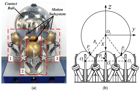
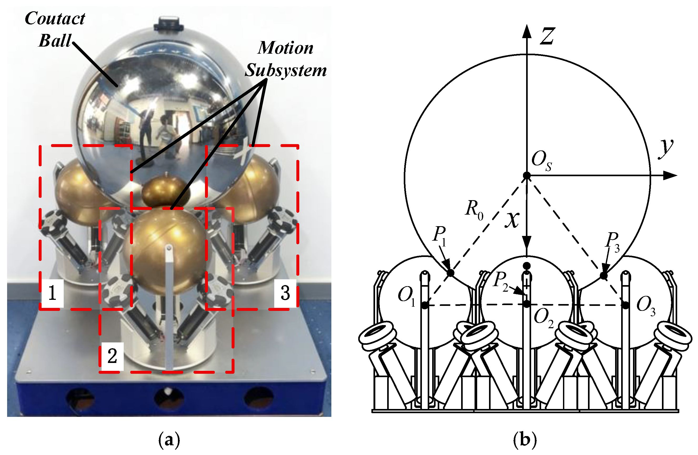
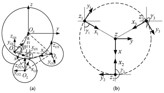
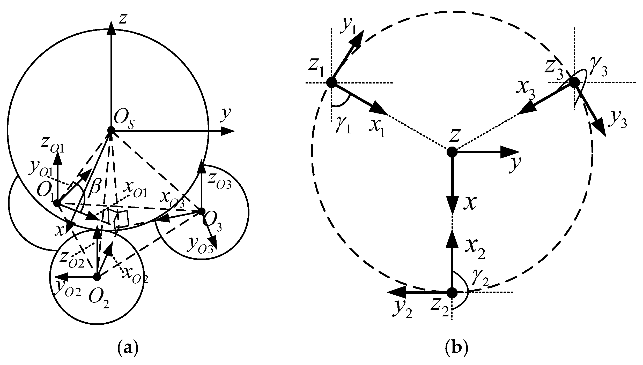
Figure 4a shows the prototype of the spherical end-effector, which primarily consists of a contact sphere and three uniformly distributed driving subsystems 1,2,3. The geometric centers of these driving subsystems are defined as ${\mathit{O}}_{\mathit{i}}\left(\mathit{i} = 1,2,3\right)$. Figure 4b presents the simplified schematic of the spherical end-effector. The geometric center and radius of the contact sphere are defined as ${\mathit{O}}_{\mathit{S}}$ and ${\mathit{R}}_0$, respectively. A coordinate system is established with ${\mathit{O}}_{\mathit{S}}$ as the origin: the X-axis points outward perpendicular to the current view, the Y-axis points horizontally to the right parallel to the view, and the Z-axis points vertically upward. The contact points between the driving subsystems and the contact sphere are denoted as ${\mathit{P}}_{\mathit{i}}\left(\mathit{i} = 1,2,3\right)$.

Figure 4. Spherical end-effector: (a) Prototype; (b) Simplified schematic.

Figure 5a presents an axonometric view of the simplified schematic of the spherical end-effector. Coordinate frames ${\mathit{O}}_{\mathit{i}}\left(\mathit{i} = 1,2,3\right)$ are established with the geometric centers of the driven spheres as their respective origins. As shown in Figure 5a, the X-axis of each ${\mathit{O}}_{\mathit{i}}\left(\mathit{i} = 1,2,3\right)$ frame points toward the center of the contact sphere and forms an angle ${\mathsf{\gamma }}_{\mathit{i}}\left(\mathit{i} = 1,2,3\right)$ with a dashed line parallel to the downward direction of the current view. The Z-axis of each ${\mathit{O}}_{\mathit{i}}\left(\mathit{i} = 1,2,3\right)$ frame points vertically upward and is parallel to the Z-axis of the ${\mathit{O}}_{\mathit{S}}$ frame.

Figure 5. Spherical end-effector: (a) Axonometric schematic; (b) Top-view kinematic diagram.

2.3.2. Kinematic of the System

With respect to the ${\mathit{O}}_{\mathit{s}}$ coordinate frame, the velocity ${\mathit{v}}_{\mathit{opi}}\left(\mathit{i} = 1,2,3\right)$ of the contact point ${\mathrm{P}}_{\mathrm{i}}\left(\mathit{i} = 1,2,3\right)$ on the driven sphere ${\mathit{O}}_{\mathit{i}}$ is expressed as Equation (27):

$${\mathit{v}}_{\mathit{opi}} = {\dot{\mathit{x}}}_{\mathit{oi}} + {\dot{\mathbf{\Theta }}}_{\mathit{oi}}^{\mathit{s}} \times \left(\mathit{R}{\mathit{n}}_{\mathit{oi}}\right)\left(\mathit{i} = 1,2,3\right)$$

(27)

where ${\dot{\mathit{x}}}_{\mathit{oi}} \mathsf{ϵ} {\mathbf{R}}^{\mathbf{3}}$ represents the translational velocity of the driven sphere ii with respect to the ${\mathit{O}}_{\mathit{s}}$ coordinate frame; ${\dot{\mathbf{\Theta }}}_{\mathit{oi}}^{\mathit{s}} \mathsf{ϵ}{ \mathbf{R}}^{\mathbf{3}}$ denotes its angular velocity about the coordinate axes relative to the ${\mathit{O}}_{\mathit{s}}$ frame; and ${\mathit{n}}_{\mathit{oi}} \mathbf{ϵ}{ \mathbf{R}}^{\mathbf{3}}$ is the position vector from the geometric center ${\mathit{O}}_{\mathit{i}}\left(\mathit{i} = 1,2,3\right)$ to the corresponding contact point ${\mathrm{P}}_{\mathrm{i}}\left(\mathit{i} = 1,2,3\right)$.

Similarly, with respect to the ${\mathit{O}}_{\mathit{s}}$ coordinate frame, the velocity ${\mathit{v}}_{\mathit{ospi}}\left(\mathit{i} = 1,2,3\right)$ of the contact point ${\mathit{P}}_{\mathit{i}}$ on the large sphere ${\mathit{O}}_{\mathit{s}}$ is expressed as Equation (28):

$${\mathit{v}}_{\mathit{ospi}} = {\dot{\mathit{x}}}_{\mathit{os}} + {\dot{\mathbf{\Theta }}}_{\mathit{os}}^{\mathit{s}} \times \left({\mathit{R}}_{\mathit{s}}{\mathit{n}}_{\mathrm{osi}}\right)\left(\mathit{i} = 1,2,3\right)$$

(28)

where ${\dot{\mathit{x}}}_{\mathit{os}} \mathbf{ϵ}{ \mathbf{R}}^{\mathbf{3}}$ represents the translational velocity of the contact sphere with respect to the ${\mathit{O}}_{\mathit{s}}$ coordinate frame; ${\dot{\mathbf{\Theta }}}_{\mathit{os}}^{\mathit{s}} \mathbf{ϵ} {\mathbf{R}}^{\mathbf{3}}$ denotes its angular velocity about the coordinate axes relative to the ${\mathit{O}}_{\mathit{s}}$ frame; and ${\mathit{n}}_{\mathrm{osi}} \mathbf{ϵ} {\mathbf{R}}^{\mathbf{3}}$ is the position vector from the geometric center ${\mathit{O}}_{\mathit{s}}$ to the corresponding contact point ${\mathrm{P}}_{\mathrm{i}}\left(\mathit{i} = 1,2,3\right)$.

Since the motion between the spheres involves pure rolling contact without relative sliding, the relationship expressed in Equation (29) holds:

$${\mathit{v}}_{\mathit{opi}} ={ \mathit{v}}_{\mathit{ospi}}(\mathit{i} = 1,2,3)$$

(29)

That is, Equation (30) holds:

$${\dot{\mathit{x}}}_{\mathit{oi}}+{\dot{\mathbf{\Theta }}}_{\mathit{oi}}^{\mathit{s}} \times \left(\mathit{R}{\mathit{n}}_{\mathit{oi}}\right) = {\dot{\mathit{x}}}_{\mathit{os}} + {\dot{\mathbf{\Theta }}}_{\mathit{os}}^{\mathit{s}} \times \left({\mathit{R}}_{\mathit{s}}{\mathit{n}}_{\mathit{osi}}\right)(\mathit{i} = 1,2,3)$$

(30)

Constrained by the structural configuration of the spherical end-effector, neither the driven spheres 1,2,3 nor the contact sphere undergoes translational motion. Therefore, Equation (31) always holds:

$${\dot{\mathit{x}}}_{\mathit{oi}} \equiv {\dot{ \mathit{x}}}_{\mathit{os}} \equiv 0(\mathit{i} = 1,2,3)$$

(31)

Combining Equation (26), Equation (25) can be further simplified as Equation (32):

$${\dot{\mathbf{\Theta }}}_{\mathit{oi}}^{\mathit{s}} \times \left(\mathit{R}{\mathit{n}}_{\mathrm{oi}}\right) ={\dot{ \mathbf{\Theta }}}_{\mathit{os}}^{\mathit{s}} \times \left({\mathit{R}}_{\mathit{s}}{\mathit{n}}_{\mathit{osi}}\right)(\mathit{i} = 1,2,3)$$

(32)

Since the points ${\mathit{O}}_{\mathit{i}},{\mathit{P}}_{\mathit{i}},{\mathit{O}}_{\mathit{s}}$ are collinear, Equation (33) is evidently satisfied:

$${\mathit{n}}_{\mathit{oi}} = -{\mathit{n}}_{\mathit{osi}}(\mathit{i} = 1,2,3)$$

(33)

Combining Equations (32) and (33) yields Equation (34):

$${\dot{\mathbf{\Theta }}}_{\mathit{oi}}^{\mathit{s}}\mathit{R} = -{\dot{\mathbf{\Theta }}}_{\mathit{os}}^{\mathit{s}}{\mathit{R}}_{\mathit{s}}(\mathit{i} = 1,2,3)$$

(34)

From Equation (34), the relationship shown in Equation (35) can be evidently obtained:

$${\dot{\mathbf{\Theta }}}_{\mathit{o}\mathbf{1}}^{\mathit{S}} = {\dot{\mathbf{\Theta }}}_{\mathit{o}\mathbf{2}}^{\mathit{S}} = {\dot{\mathbf{\Theta }}}_{\mathit{o}\mathbf{3}}^{\mathit{S}}$$

(35)

Equation (35) indicates that, within the same ${\mathit{O}}_{\mathit{s}}$ coordinate frame, the motion of each driven sphere must remain consistent at all times. This fully demonstrates that, from a kinematic perspective, the multi-driven spheres constitute an equal-angular-velocity system with multiple inputs and rigid coupling. The advantages of this design are twofold: First, the multi-support configuration can provide sufficient supporting force; Second, it satisfies the requirements for redundant backup. In harsh space environments, spacecraft surfaces are frequently subjected to impacts from space debris. Furthermore, the complex and diverse radiation in space makes electronic components highly susceptible to single-event effects, which can lead to functional failures.

Using the transformation matrix given in Equation (36), the angular velocities of the driven spheres ${\dot{\mathbf{\Theta }}}_{\mathit{oi}}^{\mathit{s}}\left(\mathit{i} = 1,2,3\right)$, with respect to the ${\mathit{O}}_{\mathit{s}}$ frame, can be transformed into their corresponding angular velocities ${\dot{\mathbf{\Theta }}}_{\mathit{oi}}^{\mathit{o}}\left(\mathit{i} = 1,2,3\right)$ relative to the individual coordinate frames ${\mathit{O}}_{\mathit{i}}\left(\mathit{i} = 1,2,3\right)$, as expressed in Equation (32):

$${\mathit{Rot}}_{\mathit{z}}\left({\mathsf{\gamma }}_{\mathit{i}}\right) = \left[\begin{array}{ccc}\mathit{cos}\left({\mathsf{\gamma }}_{\mathit{i}}\right)& -\mathit{sin}\left({\mathsf{\gamma }}_{\mathit{i}}\right)& 0\\ \mathit{sin}\left({\mathsf{\gamma }}_{\mathit{i}}\right)& \mathit{cos}\left({\mathsf{\gamma }}_{\mathit{i}}\right)& 0\\ 0& 0& 1\end{array}\right]$$

(36)

$${\dot{\mathbf{\Theta }}}_{\mathit{oi}}^{\mathit{o}}={{ \mathit{Rot}}_{\mathit{z}}\left({\mathsf{\gamma }}_{\mathit{i}}\right)}^{\mathit{T}}{\dot{\mathbf{\Theta }}}_{\mathit{oi}}^{\mathit{s}}(\mathit{i}=1,2,3)$$

(37)

Combining Equations (36) and (37), the kinematic mapping relationship between each Omniwheel and the contact sphere can be obtained, as expressed in Equation (38):

$${\dot{\mathbf{\Theta }}}_{\mathit{os}}^{\mathit{s}} = {\displaystyle \frac{\frac{{\mathit{r}}_{\mathit{\omega }}}{\mathit{R}}{\left({\mathit{B}\left({\mathit{\theta }}_{\mathit{i}},\mathit{\alpha }\right)}^{\mathit{T}}\mathit{B}\left({\mathit{\theta }}_{\mathit{i}},\mathit{\alpha }\right)\right)}^{-1}{\mathit{B}\left({\mathit{\theta }}_{\mathit{i}},\mathit{\alpha }\right)}^{\mathit{T}}{\mathit{\omega }}^{\mathit{i}}}{{{\mathit{Rot}}_{\mathit{z}}\left({\mathsf{\gamma }}_{\mathit{i}}\right)}^{\mathit{T}}}}(\mathit{i} = 1,2,3)$$

(38)

2.3.3. Dynamics of the Spherical End-Effector

The dynamic analysis of the spherical end-effector extends the kinematic coupling in Section 2.3.2 to include torque transmission. For each driving subsystem j (j = 1,2,3), the rotational dynamics of the driven sphere in its local coordinate frame ${\mathit{O}}_{\mathit{j}}$ is governed by the Euler equation:

$${\mathit{I}}_{\mathit{o}}{\dot{\mathit{\omega }}}_{\mathit{o},\mathit{j}}^{\mathit{o}} = {\mathit{\tau }}_{\mathit{w},\mathit{j}}^{\mathit{o}}$$

(39)

where ${\mathit{\tau }}_{\mathit{w},\mathit{j}}^{\mathit{o}}$ is the net driving torque exerted by the three omniwheels on the j-th driven sphere, and the gyroscopic term vanishes due to the spherical symmetry of the driven sphere.

Transforming the torque to the ${\mathit{O}}_{\mathit{s}}$ frame via the rotation matrix in Equation (36):

$${\mathit{\tau }}_{\mathit{w},\mathit{j}}^{\mathit{s}} = {\mathbf{Rot}}_{\mathit{z}}({\mathsf{\gamma }}_{\mathit{j}}) {\mathit{\tau }}_{\mathit{w},\mathit{j}}^{\mathit{o}}$$

(40)

Owing to the constraint Equation (35), the angular velocities of all three driven spheres in the ${\mathit{O}}_{\mathit{s}}$ frame are identical and kinematically coupled to the contact sphere by Equation (34):

$${\mathit{\omega }}_{\mathit{o},\mathit{j}}^{\mathrm{s}} = -{\displaystyle \frac{{\mathrm{R}}_{\mathrm{s}}}{\mathrm{R}}}{\mathit{\omega }}_{\mathit{o}\mathit{s}},j=1,2,3$$

(41)

Differentiating with respect to time yields:

$${\dot{\mathit{\omega }}}_{\mathit{o},\mathit{j}}^{\mathrm{s}} = -{\displaystyle \frac{{\mathrm{R}}_{\mathrm{s}}}{\mathrm{R}}}{\dot{\mathit{\omega }}}_{\mathit{o}\mathit{s}}$$

(42)

Substituting into Equation (39) and transforming via Equation (40) gives the driving torque of each subsystem expressed in the ${\mathit{O}}_{\mathit{s}}$ frame:

$${\mathit{\tau }}_{\mathit{w},\mathit{j}}^{\mathit{s}} = -{\displaystyle \frac{{\mathit{R}}_{\mathit{s}}}{\mathit{R}}}{\mathit{I}}_{\mathit{o}}{\dot{\mathit{\omega }}}_{\mathit{os}}$$

(43)

At the contact point ${\mathit{P}}_{\mathit{j}}$, the driven sphere exerts a tangential friction force on the contact sphere. Because the contact points are collinear with the centers ${\mathit{O}}_{\mathit{j}}$ and ${\mathit{O}}_{\mathit{s}}$, the torque arm ratio between the contact sphere and the driven sphere equals ${\displaystyle \frac{{\mathit{R}}_{\mathit{s}}}{\mathit{R}}}$.

Consequently, the torque transmitted from the j-th driven sphere to the contact sphere is amplified by this geometric ratio:

$${\mathbf{M}}_{\mathit{drive},\mathit{j}} = {\displaystyle \frac{{\mathit{R}}_{\mathit{s}}}{\mathit{R}}}{\mathit{\tau }}_{\mathit{w},\mathit{j} }^{\mathit{s}}= -{\left({\displaystyle \frac{{\mathit{R}}_{\mathit{s}}}{\mathit{R}}}\right)}^2{\mathit{I}}_{\mathit{o}}{\dot{\mathit{\omega }}}_{\mathit{os}}$$

(44)

Summing over the three driving subsystems, the total driving torque applied to the contact sphere is:

$${\mathbf{M}}_{\mathit{drive}}={\sum }_{\mathit{j}=1}^3{\mathbf{M}}_{\mathit{drive},\mathit{j}} = -3{\left({\displaystyle \frac{{\mathit{R}}_{\mathit{s}}}{\mathit{R}}}\right)}^2{\mathit{I}}_{\mathit{o}}{\dot{\mathit{\omega }}}_{\mathit{os}}$$

(45)

The rotational dynamics of the contact sphere, with inertia ${\mathit{I}}_{\mathit{s}} ={\displaystyle \frac{ 2}{5}}{\mathit{m}}_{\mathit{s}}{\mathit{R}}_{\mathit{s}}^2$, is then:

$${\mathit{I}}_{\mathit{s}}{\dot{\mathit{\omega }}}_{\mathit{s}} ={ \mathbf{M}}_{\mathit{drive}}-{\mathbf{M}}_{\mathit{contact}}$$

(46)

where ${\mathbf{M}}_{\mathit{contact}}$ is the contact torque exerted by the non-cooperative target on the contact sphere. Equation (46) establishes the dynamic balance between the driving torque generated by the nine omniwheels and the reaction torque from the target.

3. Experiments

In Section 2, the structural composition, geometric relationships, transmission process, and coordinate system definitions of the driving subsystem and the spherical end-effector were elaborated in detail. Based on the preceding content, this section primarily aims to validate the correctness of the theoretical kinematic calculations and assess the feasibility of motion control for such mechanisms through a comparative analysis involving theoretical calculations, simulation experiments, and physical prototype verification.

3.1. Experiment of the Driving Subsystem

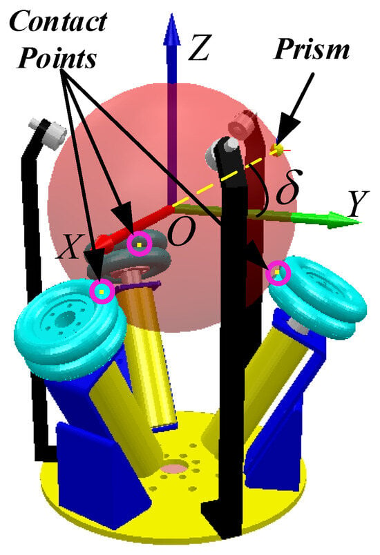
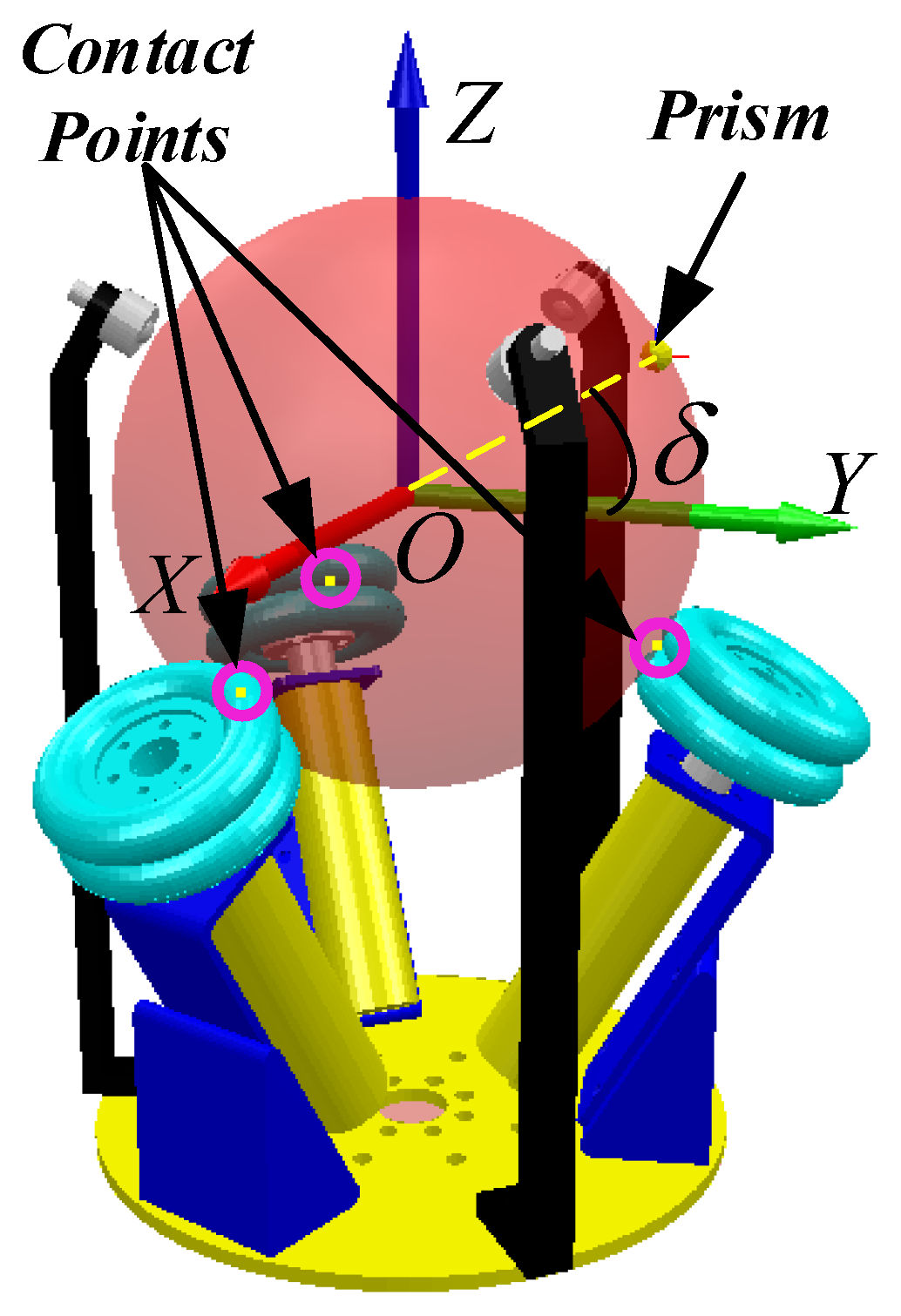
Taking driving subsystem 1 as an example, a simulation model was established using the CoppeliaSim 4.10 software, as shown in Figure 6. A prism is mounted on the surface of the driven sphere within the YOZ plane at an angle δ from the positive Y-axis direction. This prism can be utilized to measure variations in the motion of the driven sphere. Combined with the contact monitoring function of the CoppeliaSim software, the positions and contact states between the driven sphere and each OmniWheel are displayed in real time. The contact points are represented by yellow dots enclosed within pink circles in Figure 6. By employing this contact monitoring mechanism, it is possible to determine whether separation occurs between the sphere and the wheels during motion. If separation occurs, it indicates discontinuous motion; conversely, the motion is considered normal.

Figure 6. Simulation model of driving subsystem 1.

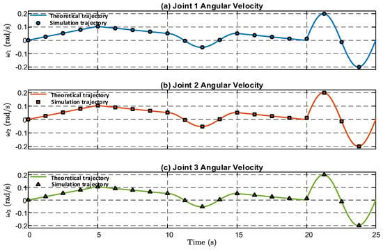
Based on the MATLAB 2024a software, the equations in Equation (21) were formulated. The input-output mapping relationship of the equations was compared with the simulation results to verify the correctness of Equation (21). First, the feasibility and stability of the simulation model itself were validated. Within a time span of 0 to 25 s, the OmniWheels were controlled to rotate at the angular velocities specified in Table 1. During this process, the rotational speeds of each wheel in the simulation model were recorded and sampled at 1-s intervals. Finally, the variation curves of the theoretical rotational speeds and the interval-sampled simulation rotational speeds were plotted, as shown in Figure 7.

Table 1. Angular Velocity of OmniWheel Motion.

Time(s)	0~5	5~10	10~15	15~20	20~25
Wheel 1 velocity(rad/s)	0 → ${\displaystyle \frac{\mathsf{\pi }}{6}}$	${\displaystyle \frac{\mathsf{\pi }}{6}}\to {\displaystyle \frac{\mathsf{\pi }}{12}}$	${\displaystyle \frac{\mathsf{\pi }}{12}}\to {\displaystyle \frac{\mathsf{\pi }\mathit{cos}\left(\mathrm{t}\right)}{12}}$	${\displaystyle \frac{\mathsf{\pi }\mathit{cos}\left(\mathrm{t}\right)}{12}}\to 0$	$0\to {\displaystyle \frac{\mathsf{\pi }\sin \left(\mathrm{t}\right)}{6}}$
Wheel 2 velocity(rad/s)	0 → ${\displaystyle \frac{\mathsf{\pi }}{6}}$	${\displaystyle \frac{\mathsf{\pi }}{6}}\to {\displaystyle \frac{\mathsf{\pi }}{12}}$	${\displaystyle \frac{\mathsf{\pi }}{12}}\to {\displaystyle \frac{\mathsf{\pi }\mathit{cos}\left(\mathrm{t}\right)}{12}}$	${\displaystyle \frac{\mathsf{\pi }\mathit{cos}\left(\mathrm{t}\right)}{12}}\to 0$	$0\to {\displaystyle \frac{\mathsf{\pi }\sin \left(\mathrm{t}\right)}{6}}$
Wheel 3 velocity(rad/s)	0 → ${\displaystyle \frac{\mathsf{\pi }}{6}}$	${\displaystyle \frac{\mathsf{\pi }}{6}}\to {\displaystyle \frac{\mathsf{\pi }}{12}}$	${\displaystyle \frac{\mathsf{\pi }}{12}}\to {\displaystyle \frac{\mathsf{\pi }\mathit{cos}\left(\mathrm{t}\right)}{12}}$	${\displaystyle \frac{\mathsf{\pi }\mathit{cos}\left(\mathrm{t}\right)}{12}}\to 0$	$0\to {\displaystyle \frac{\mathsf{\pi }\sin \left(\mathrm{t}\right)}{6}}$

Figure 7. Velocity Operation Curves.

In Figure 7, the x-axis denotes the operation time in seconds, while the y-axis denotes the angular velocity of each omniwheel. The solid lines represent the theoretical trajectories computed from the inverse kinematic model, and the discrete markers represent the simulation trajectories sampled at 1s intervals. As shown in Figure 7, the interval-sampled simulation rotational speeds are in perfect agreement with the theoretical rotational speeds. This demonstrates that the simulation results are reliable, confirming that the simulation model was correctly established and that the OmniWheels can operate at the expected angular velocities.

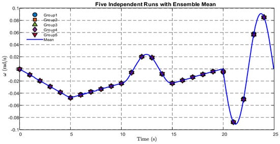
Next, the stability of the simulation model was validated. Specifically, the OmniWheels in the simulation model were driven to complete five full motion cycles according to the angular velocity values specified in Table 1. The angular velocity of the driven sphere rotating about the Z-axis, with reference to coordinate system $\mathit{O}$, was recorded for each cycle, as shown in Figure 8. In Figure 8 the x-axis represents time in seconds, and the y-axis represents angular velocity in radians per second. The five discrete marker sets denote the individual experimental runs (Group 1 to Group 5), and the blue solid line denotes the ensemble mean. In Figure 8, the five types of markers represent the angular velocities of the driven sphere during the first through fifth rotations about the Z-axis, while the blue solid line indicates the average value of these five sets of data.

Figure 8. Rotation Angle of the Driven Sphere.

Based on Equation (47), Equation (48), and Equation (49), the Mean SD, Mean CV, and Mean SEM of the aforementioned data were calculated, respectively, and the results are summarized in Table 2.

$${\mathit{SD}}_{\mathit{i}}=\sqrt{{\displaystyle \frac{1}{\mathit{M}-1}}{\displaystyle \sum _{\mathit{j}=1}^{\mathit{j}=\mathit{M}}}{\left({\mathit{x}}_{\mathit{ij}}-{\overline{\mathit{x}}}_{\mathit{i}}\right)}^2}$$

(47)

where ${\mathit{SD}}_{\mathit{i}}$ represents the standard deviation, reflecting the absolute fluctuation magnitude of the data; i denotes the i-th data point; j denotes the j-th data group; M represents the total number of data groups; ${\mathit{x}}_{\mathit{ij}}$ represents the i-th data point in the j-th group; and ${\overline{\mathit{x}}}_{\mathit{i}}$ represents the mean value of the i-th data point.

$$\mathit{Mean} \mathit{SD}={\displaystyle \frac{1}{\mathit{N}}}{\sum }_{\mathit{i}=1}^{\mathit{i}=\mathit{N}}{\mathit{SD}}_{\mathit{i}}$$

(48)

where $\mathit{Mean} \mathit{SD}$ represents the average of the standard deviations, which can be used to measure the absolute deviation of the data; ii denotes the standard deviation of the i-th data point; and N is the total number of data groups.

$${\mathit{CV}}_{\mathit{i}}={\displaystyle \frac{{\mathit{SD}}_{\mathit{i}}}{{\overline{\mathit{x}}}_{\mathit{i}}}} \times 100\%$$

(49)

where ${\mathit{CV}}_{\mathit{i}}$ represents the coefficient of variation, reflecting the degree of dispersion for data with different magnitudes.

$$\mathit{Mean} \mathit{CV}={\displaystyle \frac{1}{\mathit{N}}}{\sum }_{\mathit{i}=1}^{\mathit{i}=\mathit{N}}{\mathit{CV}}_{\mathit{i}}$$

(50)

where $\mathit{Mean} \mathit{CV}$ represents the average of the coefficients of variation, which can be used to measure the relative fluctuation of the data.

$${\mathit{SEM}}_{\mathit{i}}={\displaystyle \frac{{\mathit{SD}}_{\mathit{i}}}{\mathit{M}}}$$

(51)

where ${\mathit{SEM}}_{\mathit{i}}$ represents the standard error of the mean, reflecting the precision with which the sample mean estimates the population mean.

$$\mathit{Mean} \mathit{SEM}={\displaystyle \frac{1}{\mathit{N}}}{\sum }_{\mathit{i}=1}^{\mathit{i}=\mathit{N}}{\mathit{SEM}}_{\mathit{i}}$$

(52)

where $\mathit{Mean} \mathit{SEM}$ represents the average of the standard errors of the mean, which can be used to measure the reliability of the mean values.

Table 2. Calculation Results.

	Mean SD	Mean CV	Mean SEM
Value	2.71 × 10−4	3.06%	1.22 × 10−4

The mean standard deviation (SD) of the data is 2.71 × 10⁻⁴, the mean coefficient of variation (CV) is 3.06%, and the mean standard error of the mean (SEM) is 1.22 × 10⁻⁴. These results indicate that the simulated trajectory is in high agreement with the theoretical trajectory, demonstrating a high level of reliability in the simulation.

Next, Equation (22) was validated through theoretical calculations, simulation modeling, and physical motion control. Specifically, the positions of the prism under these three conditions were recorded, as shown in Figure 9. In Figure 9, the horizontal axes denote the X and Y positions in meters, and the vertical axis denotes the Z position in meters. The blue solid line represents the theoretical trajectory, the orange solid line represents the simulation trajectory, and the green solid line represents the physical prototype trajectory.

$$\mathit{RMSE}=\sqrt{{\displaystyle \frac{1}{\mathit{n}}}{\sum }_{\mathit{i}=1}^{\mathit{n}}{‖{\mathit{p}}_{\mathit{i}}-\widehat{{\mathit{p}}_{\mathit{i}}}‖}^2}$$

(53)

where n is the number of points; ${\mathit{p}}_{\mathit{i}}$ is the actual position of the i-th point; $\widehat{{\mathit{p}}_{\mathit{i}}}$ is the estimated position of the i-th point.

Figure 9. Motion Trajectories of the Prism Under Three Conditions.

The root mean square errors (RMSEs) for the overlaps between the theoretical and simulated trajectories, as well as between the theoretical and physical trajectories, are 4.082 × 10⁻⁴ and 0.0032, respectively. These results demonstrate that the simulated trajectory is in high agreement with the theoretical one, proving that the established kinematic model can accurately describe the ideal behavior of the system. The physical error is approximately eight times greater than the simulation error. This discrepancy may primarily originate from sensor measurement noise, mechanical transmission backlash, and environmental disturbances. Ultimately, this level of accuracy meets the requirements of practical engineering applications.

3.2. Spherical End-Effector Experiment

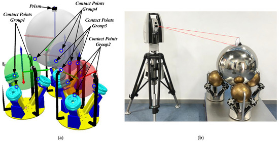
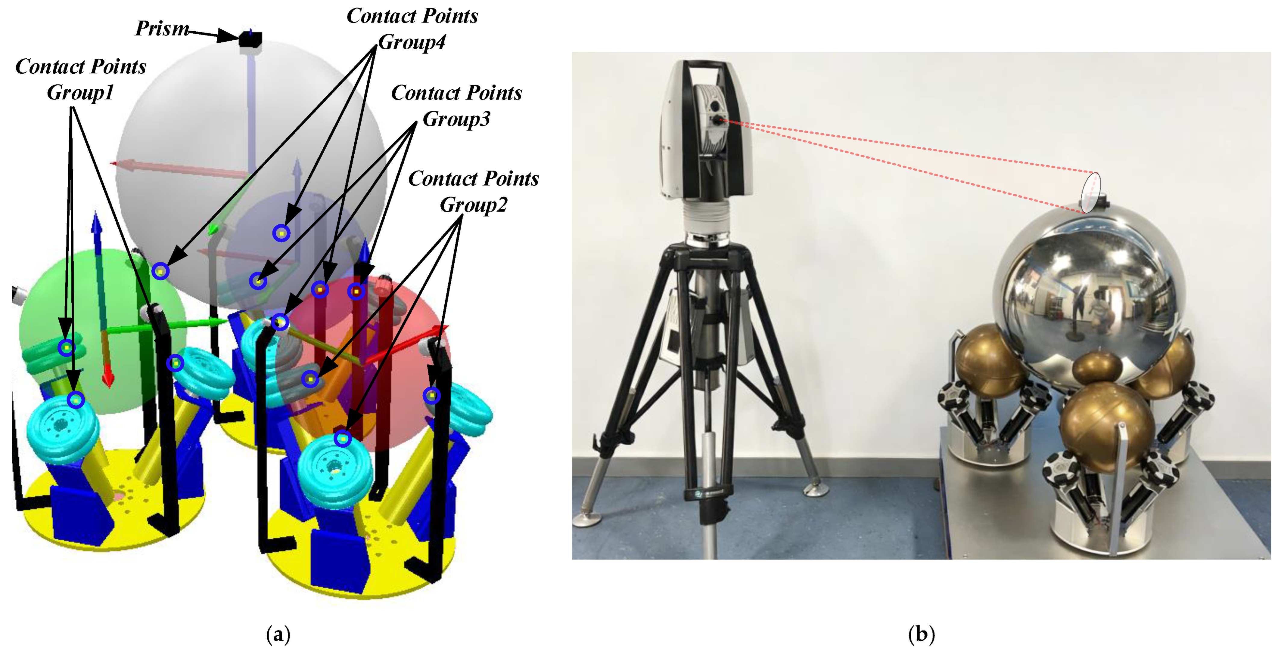
The previous section used Drive Subsystem 1 as an example to verify the reliability of the kinematic modeling, the simulation model, and the feasibility of physical motion control. This section will focus on validating the spherical end-effector. First, a simulation model of the spherical end-effector was established, as shown in Figure 10a. This model consists of three evenly distributed drive subsystems and a contact sphere. A prism is mounted at the intersection of the Z-axis of the contact sphere’s coordinate system and its surface to monitor its motion. Combined with the contact monitoring function of the CoppeliaSim software, the drive subsystem itself and the contact points between the driving spheres and the contact sphere can be displayed in real time to detect any detachment during movement. Subsequently, a physical prototype testing system was constructed, primarily comprising a Leica Laser Tracker System and the spherical end-effector. As illustrated in Figure 10b, the Leica tracker measures the position of the prism on the spherical end-effector in real time to reflect the dynamic changes in the motion of the contact sphere.

Figure 10. Spherical end-effector: (a) Simulation model; (b) Experimental testing system.

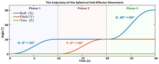
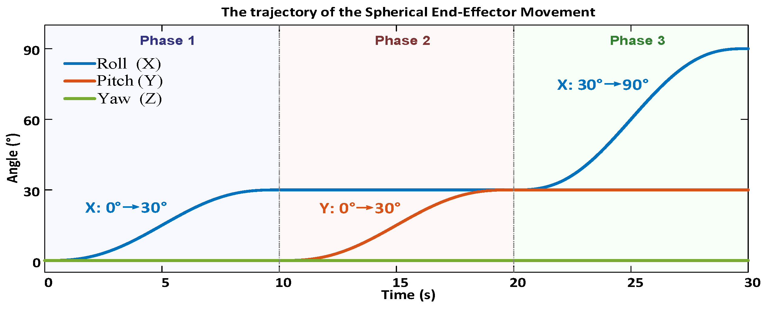
Equation (38) reflects the mapping relationship between the Omniwheel and the contact sphere. Based on this mapping, the motion trajectory of the contact sphere is designed, as shown in Figure 11. In Figure 11, the x-axis represents time in seconds, and the y-axis represents the rotation angle in degrees. The motion sequence is divided into three phases: Phase 1 (0–10 s), rotation about the X-axis (Roll) from 0° to 30°; Phase 2 (10–20 s), rotation about the updated Y-axis (Pitch) from 0° to 30°; and Phase 3 (20–30 s), rotation about the updated X-axis (Roll) from 30° to 90°. The trajectory in Figure 11 is represented by rotations around the moving coordinate system of the sphere. Specifically, from 0 to 10 s, the contact sphere rotates about its own X-axis from 0° to 30°. From 10 to 20 s, it rotates about the updated Y-axis from 0° to 30°. Finally, from 20 to 30 s, it rotates about the updated X-axis from 30° to 90°.

Figure 11. Desired angular motion commands.

Both the simulation model and the physical prototype were commanded to execute the aforementioned trajectory five times. The position of the prism was recorded for each run, and the RMSEs were calculated to be 6.21 × 10⁻⁵ and 8.2 × 10⁻⁴, respectively. The results indicate that the simulation model exhibits minimal motion fluctuation and high reliability. Although the error of the physical prototype is approximately 13 times greater than that of the simulation, with correspondingly larger fluctuations, it remains within an acceptable range.

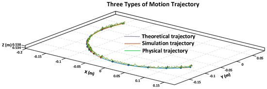
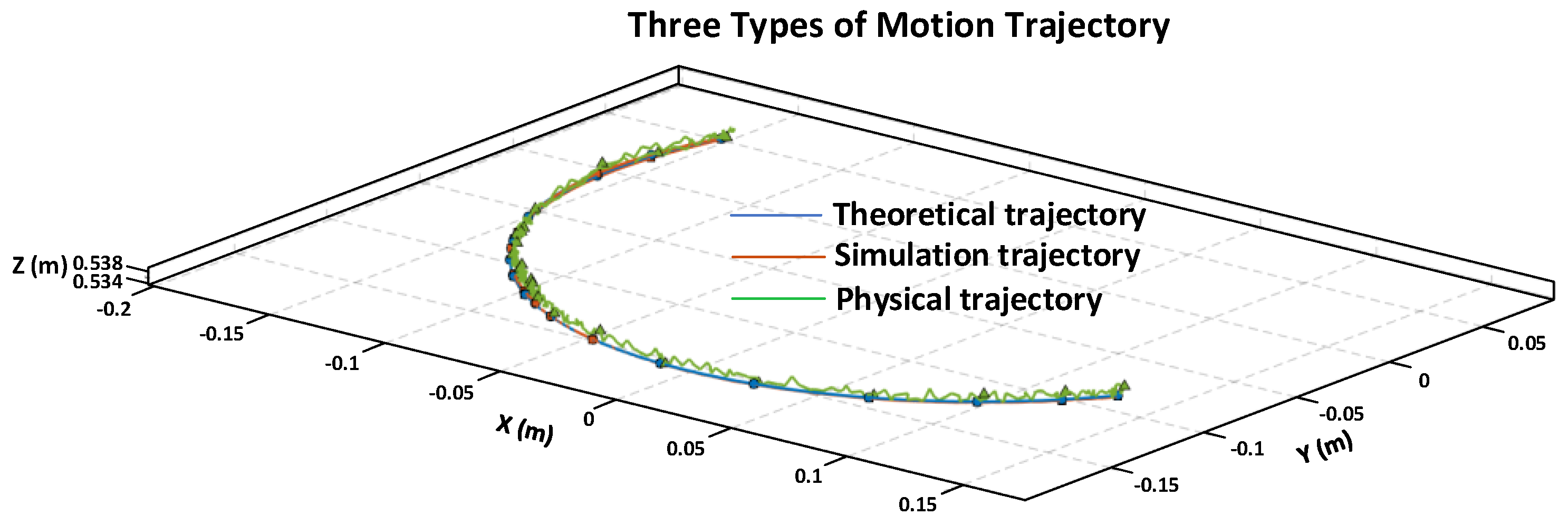
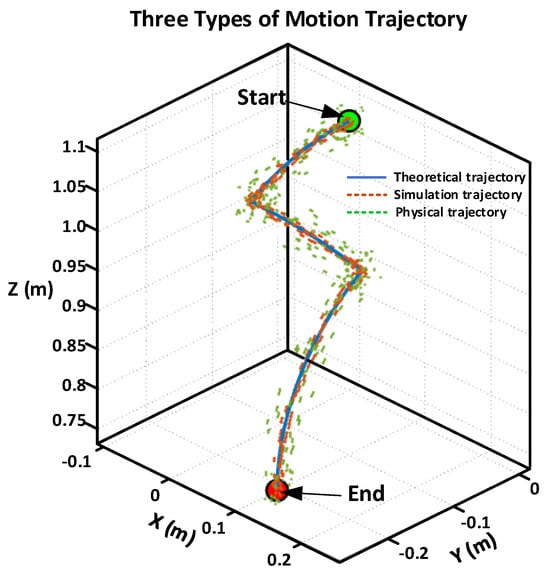
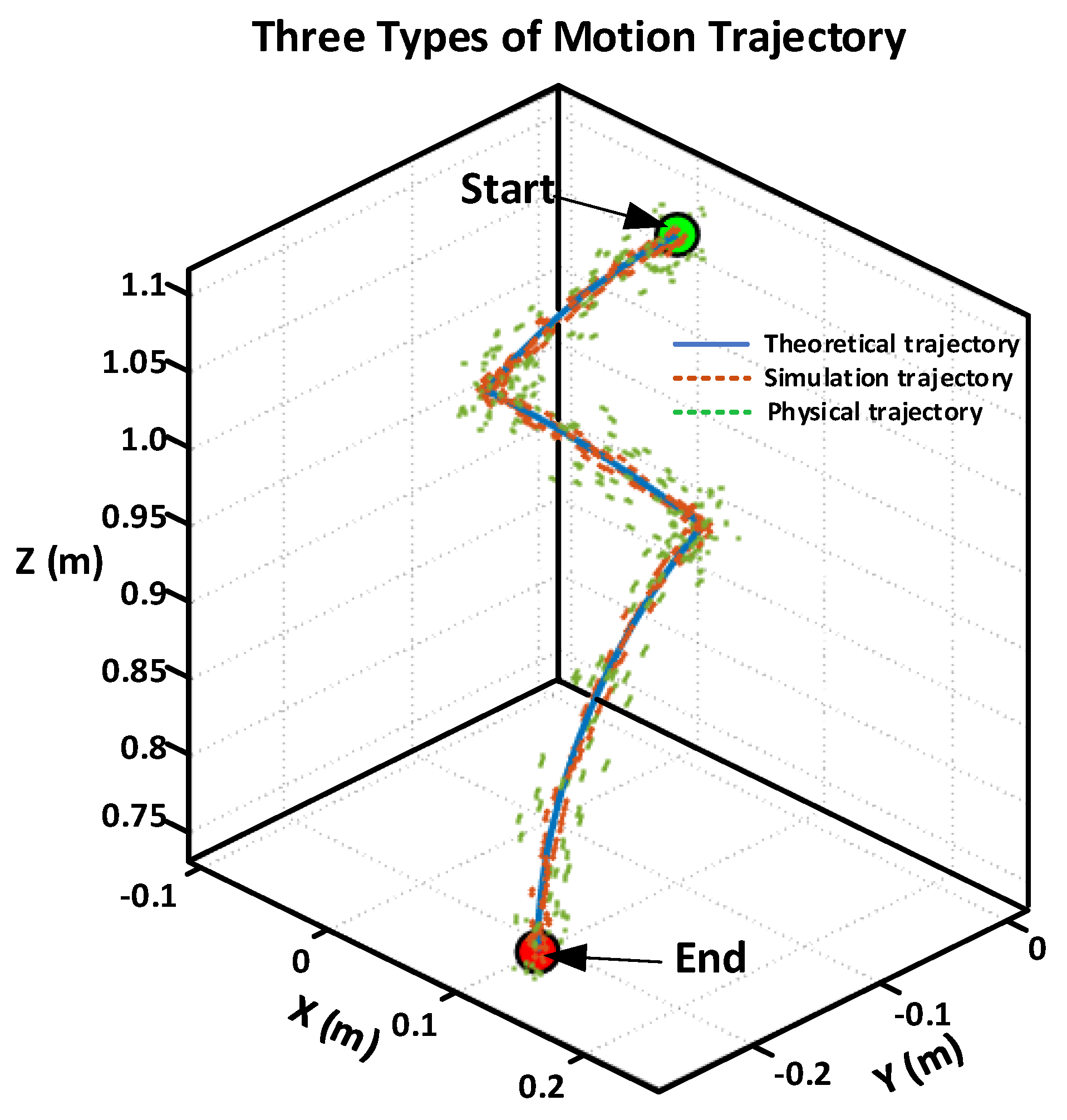
The positions of the prism under the aforementioned motion conditions were recorded and plotted for the theoretical calculation, the simulation model, and the physical prototype, as shown in Figure 12. In Figure 12, the x-axis and y-axis, respectively, represent the X and Y positions in meters, and the z-axis represents the Z position in meters. The blue solid line denotes the theoretical trajectory, the orange dash-dotted line denotes the simulation trajectory, and the green dashed line denotes the physical prototype trajectory. The green and red circles indicate the start and end points, respectively.

Figure 12. Motion trajectories.

The RMSEs between the theoretical model and the simulation model, as well as between the theoretical model and the physical prototype, were calculated to be 0.0929 and 1.62, respectively. The results indicate that the simulated trajectory highly coincides with the theoretical one, demonstrating that the established kinematic model can accurately describe the ideal behavior of the system. Although the error of the physical prototype is approximately 17 times greater than that of the simulation, which has increased compared to a single drive subsystem due to the addition of transmission components, the overall error remains relatively small and is still acceptable.

3.3. Engineering Significance of the Reported Errors

The RMSE values reported above should be interpreted in the context of practical engineering requirements. For the driving subsystem, the RMSE of 4.082 × 10⁻⁴ (theory vs. simulation) and 0.0032 (theory vs. physical prototype) represent negligible deviations in angular velocity. In precision drive systems, such error levels are well within acceptable tolerances, considering inherent mechanical backlash, sensor noise, and motor control quantization. The close agreement between simulation and physical prototype validates both the kinematic model and the manufacturing fidelity. For the spherical end-effector, the simulation RMSE of 0.0929 demonstrates that the derived kinematic mapping Equation (38) accurately describes the ideal system behavior. The physical prototype RMSE of 1.62, while larger due to accumulated tolerances across three cascaded driving subsystems and measurement uncertainty from the Leica Laser Tracker, remains acceptable for the intended application. In on-orbit detumbling operations, the objective is to attenuate the target’s angular velocity from potentially high initial values to a stabilized state suitable for robotic capture. The reported error magnitude is sufficiently small relative to the mechanical engagement tolerance of the end-effector and the dynamic scale of typical space debris, thereby confirming the practical feasibility of the proposed system.

3.4. Sensitivity Analysis

To assess the robustness of the proposed kinematic model and motion control strategy under practical conditions, a comprehensive sensitivity analysis was conducted through numerical simulation based on the derived kinematic mapping Equation (38). The analysis evaluates three primary sources of uncertainty commonly encountered in physical implementation: geometric parameter deviations due to manufacturing tolerances, friction-induced slip at contact interfaces, and measurement noise in the motor control loop.

Simulation Methodology. The nominal geometric parameters are established based on the physical prototype dimensions: omniwheel radius ${\mathit{r}}_{\mathit{\omega }}$ = 15 mm, driven sphere radius $\mathit{R}$ = 45 mm, contact sphere radius ${\mathit{R}}_{\mathit{s}}$ = 120 mm, and assembly angle $\mathit{\alpha }$ = ${ 30}^{°}$. The desired trajectory for the contact sphere follows the same angular motion sequence described in Section 3.2. For each perturbation scenario, the omniwheel angular velocities are computed using the inverse kinematic mapping Equation (38) with the nominal parameters (representing the controller’s assumed model), while the actual contact sphere motion is computed using the perturbed parameters (representing the physical system with manufacturing deviations or operational variations). The RMSE is then calculated between the desired trajectory and the actual trajectory under perturbation, following the same definition as in Equation (53).

Parameter Uncertainties. Manufacturing tolerances of ±2% were introduced to each geometric parameter individually, while the controller retained the nominal values. The resulting RMSE values are summarized in Table 3. The results indicate that the system exhibits low sensitivity to radius variations (${\mathit{r}}_{\mathit{\omega }}$ and ${\mathit{R}}_{\mathit{s}}$), with relative errors below 2.1%. Notably, the driven sphere radius $\mathit{R}$ shows negligible sensitivity because the ${\displaystyle \frac{{\mathit{r}}_{\mathit{\omega }}}{\mathit{R}}}$ ratio in the control law Equation (21) remains approximately constant when the controller and physical system deviate proportionally. The assembly angle $\mathit{\alpha }$ demonstrates the lowest sensitivity (0.60–0.61%), attributed to the symmetric ${120}^{°}$ distribution of the three omniwheels, which partially compensates for individual angular deviations.

Table 3. Sensitivity to Parameter Uncertainties (±2% deviation).

Parameter	Nominal Value	Perturbed Value	RMSE	Relative Increase
${\mathit{r}}_{\mathit{\omega }\mathrm{h}}$	15	15.3	$1.48 \times { 10}^{-3}$	2%
${\mathit{r}}_{\mathit{\omega }\mathit{l}}$	15	14.7	$1.48 \times { 10}^{-3}$	2%
${\mathit{R}}_{\mathrm{h}}$	45	45.9	$\approx 0$	<0.01%
${\mathit{R}}_{\mathit{l}}$	45	44.1	$\approx 0$	<0.01%
${\mathit{R}}_{\mathit{s}\mathrm{h}}$	120	122.4	$1.45 \times { 10}^{-3}$	1.96%
${\mathit{R}}_{\mathit{sl}}$	120	117.6	$1.51 \times {10}^{-3}$	2.04%
${\mathit{\alpha }}_{\mathrm{h}}$	${30}^{°}$	${30.6}^{°}$	$4.55 \times {10}^{-4}$	0.61%
${\mathit{\alpha }}_{\mathit{l}}$	${30}^{°}$	${29.4}^{°}$	$4.41 \times { 10}^{-4}$	0.60%

Friction Variations. The pure rolling assumption in the kinematic model was relaxed by introducing velocity-dependent slip ratios δ at the contact points, defined as follows:

$$\mathsf{\delta } = {\displaystyle \frac{{\mathit{v}}_{\mathit{w}\mathrm{h}eel}-{\mathit{v}}_{\mathit{s}\mathit{p}\mathrm{h}\mathit{e}\mathit{r}\mathit{e}}}{{\mathit{v}}_{\mathit{w}\mathrm{h}\mathit{e}\mathit{e}\mathit{l}}}}$$

(54)

where ${\mathit{v}}_{\mathit{w}\mathrm{h}\mathit{e}\mathit{e}\mathit{l}}$ is the theoretical rolling velocity of the omniwheel and ${\mathit{v}}_{\mathit{s}\mathit{p}\mathrm{h}\mathit{e}\mathit{r}\mathit{e}}$ is the actual tangential velocity of the sphere at the contact point.

The slip ratio was varied from 0% to 5%. For each slip ratio, the effective omniwheel velocity was reduced by $\left(1-\mathsf{\delta }\right)$, and the resulting contact sphere motion was computed using the forward kinematic model Equation (38). The RMSE values are presented in Table 4. The results confirm a linear relationship between slip ratio and tracking error, with a 5% slip producing a 5.00% relative error. This validates the critical importance of maintaining adequate normal contact force through the constraint unit to prevent slip-induced degradation.

Table 4. Sensitivity to Friction Variations (Slip Ratio).

Slip Ratio	RMSE	Relative Increase
1%	$7.40 \times {10}^{-4}$	1%
3%	$2.22 \times { 10}^{-3}$	3%
5%	$3.70 \times {10}^{-3}$	5%

Measurement Noise. To simulate encoder quantization errors and sensor noise in the motor control loop, Gaussian white noise with standard deviations of 0.1%, 0.5%, and 1.0% of the nominal omniwheel angular velocity commands was superimposed on the velocity commands. The noise was generated using a fixed random seed to ensure reproducibility. For each noise level, the perturbed omniwheel velocities were propagated through the forward kinematic model, Equation (38), to obtain the actual contact sphere motion, and the RMSE was computed against the desired trajectory. The results are shown in Table 5. The system maintains high accuracy even at a 1.0% noise level (0.62% relative error), demonstrating the inherent noise-averaging benefit of the multi-input redundant architecture with nine omniwheels.

Table 5. Sensitivity to Measurement Noise.

Noise Level	RMSE	Relative Increase
0.1%	$4.60 \times {10}^{-5}$	0.06%
0.5%	$2.31 \times {10}^{-4}$	0.31%
1.0%	$4.62 \times { 10}^{-4}$	0.62%

The sensitivity analysis, based on numerical simulation of the derived kinematic model, confirms that the proposed system is robust against typical parameter uncertainties, moderate friction variations, and realistic measurement noise encountered in precision engineering applications. The low sensitivity to geometric deviations is attributed to the symmetric omniwheel distribution, while the linear slip-error relationship provides quantitative guidance for contact force design. The noise analysis validates the effectiveness of the redundant multi-input architecture. These findings provide practical guidance for manufacturing tolerance allocation, constraint unit force design, and sensor selection in the physical implementation of the proposed detumbling device.

4. Discussion

While this paper has established a comprehensive kinematic and dynamic modeling framework for the proposed detumbling device, several practical issues remain to be addressed to facilitate future on-orbit implementation. Specifically, the following three aspects warrant further investigation:

(1)

Rolling contact inevitably produces frictional heat. In space, where heat dissipation is poor, accumulated thermal energy may cause material degradation or thermal deformation. Future work should investigate heat generation and dissipation mechanisms under varying contact conditions.

(2)

Although the dynamic model captures basic torque transfer, the actual impact, vibration, and fluctuating contact forces encountered with targets of unknown properties require further study. This is important for refining control strategies and ensuring stable contact.

(3)

Actual detumbling experiments involving a freely rotating non-cooperative target under simulated microgravity conditions. This is the highest-priority future work, as it is essential for validating the complete detumbling performance of the proposed device in an orbital-representative environment. Our team has fabricated the physical prototype and is actively planning such experiments using an air-bearing platform.

5. Conclusions

This paper proposes an omniwheel-based active detumbling device for space debris mitigation. The kinematic mapping from nine omniwheels to the contact sphere is derived, and a dynamic model following the Lagrangian methodology is established to describe the angular momentum transfer mechanism. Experimental validation yields RMSE values of $4.082\times {10}^{-4}$ (theory vs. simulation) and 0.0032 (theory vs. prototype) for the driving subsystem, and 0.0929 and 1.62 for the spherical end-effector, confirming precise motion control capability and the feasibility of the proposed device for capturing space debris.

Current limitations include the ideal pure-rolling assumption, unquantified thermal effects from friction, and lack of microgravity validation. Future improvements will integrate force/torque sensors for adaptive preload control, develop thermo-mechanical models for heat management, and implement slip detection algorithms. Planned research directions include dynamic validation on an air-bearing platform with a freely spinning target, environmental adaptation for orbital conditions, and closed-loop system integration for autonomous detumbling and capture missions.

References

- Papadopoulos, E.; Aghili, F.; Ma, O.; Lampariello, R. Robotic Manipulation and Capture in Space: A Survey. Front. Robot. AI 2021, 8, 686723. [Google Scholar] [CrossRef] [Scilit]
- Espartero, F.; Cubas, J.; Pindado, S. Determination and Progress in Establishing the Robotic Observatory of Space Objects (ROSO). Machines 2026, 14, 532. [Google Scholar] [CrossRef] [Scilit]
- Liu, J.; Jiang, H.; Yang, X.; Li, F.; Zhao, N. Space Debris Research Progress of China. Chin. J. Space Sci. 2020, 40, 956–961. [Google Scholar] [CrossRef] [Scilit]
- Stoll, E.; Letschnik, J.; Walter, U.; Artigas, J.; Kremer, P.; Preusche, C.; Hirzinger, G. On-orbit servicing. IEEE Robot. Autom. Mag. 2009, 16, 29–33. [Google Scholar] [CrossRef] [Scilit]
- Gaias, G.; D’Amico, S.; Ardeans, J.S.; Boge, T. Hardware-in-the-loop Multi-satellite Simulator for Proximity Operations. In Proceedings of the 11th International Workshop on Simulation & EGSE Facilities for Space Programmes, Noordwijk, The Netherlands, 28–30 September 2010. [Google Scholar]
- Debus, T.; Dougherty, S. Overview and performance of the front-end robotics enabling near-term demonstration (FREND) robotic arm. In Proceedings of the AIAA Infotech@ Aerospace Conference and AIAA Unmanned...Unlimited Conference, Seattle, WA, USA, 6–9 April 2009; p. 1870. [Google Scholar]
- Lu, E.T.; Love, S.G. Gravitational tractor for towing asteroids. Nature 2005, 438, 177–178. [Google Scholar] [CrossRef] [Scilit] [PubMed]
- Bengtson, M.; Wilson, K.; Hughes, J.; Schaub, H. Survey of the electrostatic tractor research for reorbiting passive GEO space objects. Astrodynamics 2018, 2, 291–305. [Google Scholar] [CrossRef] [Scilit]
- Schaub, H.; Sternovsky, Z. Active space debris charging for contactless electrostatic disposal maneuvers. Adv. Space Res. 2014, 53, 110–118. [Google Scholar] [CrossRef] [Scilit]
- Phipps, C.R.; Baker, K.L.; Bradford, B.; George, E.V.; Libby, S.B.; Liedahl, D.A.; Marcovici, B.; Olivier, S.S.; Pleasance, L.D.; Reilly, J.P.; et al. Removing orbital debris with lasers. Adv. Space Res. 2012, 49, 1283–1300. [Google Scholar] [CrossRef] [Scilit]
- Tsuno, K.; Wada, S.; Ogawa, T.; Saito, N.; Fukushima, T.; Ebisuzaki, T.; Nakamura, Y.; Sasoh, A. Laser ablation induced impulse study for removal of space debris mission using small satellite. Appl. Phys. A 2022, 128, 932. [Google Scholar] [CrossRef] [Scilit]
- Shen, S.; Jin, X.; Hao, C. Cleaning space debris with a space-based laser system. Chin. J. Aeronaut. 2014, 27, 805–811. [Google Scholar] [CrossRef] [Scilit]
- Phipps, C.R. L’ ADROIT–A spaceborne ultraviolet laser system for space debris clearing. Acta Astronaut. 2014, 104, 243–255. [Google Scholar] [CrossRef] [Scilit]
- Ledkov, A.; Aslanov, V. Review of contact and contactless active space debris removal approaches. Prog. Aerosp. Sci. 2022, 134, 100858. [Google Scholar] [CrossRef] [Scilit]
- Yang, F.Y.; Nelson, B.; Aziz, J.; Carlino, R.; Perez, A.D.; Faber, N.; Foster, C.; Frost, C.; Henze, C.; Karacalıoğlu, A.G.; et al. LightForce photon-pressure collision avoidance: Efficiency analysis in the current debris environment and long-term simulation perspective. Acta Astronaut. 2016, 126, 411–423. [Google Scholar] [CrossRef] [Scilit] [PubMed]
- Walker, L.; Vasile, M. Space debris remediation using space-based lasers. Adv. Space Res. 2023, 72, 2786–2800. [Google Scholar] [CrossRef] [Scilit]
- Fang, Y. Influence rules of ground-based laser active removing centimeter-sized orbital debris in LEO. Optik 2018, 170, 210–219. [Google Scholar] [CrossRef] [Scilit]
- Biesbroek, R.; Soares, T.; Hüsing, J.; Innocenti, L. The e.Deorbit CDF Study: A Design Study for the Safe Removal of a Large Space Debris. In Proceedings of the 6th European Conference on Space Debris, Darmstadt, Germany, 22–25 April 2013. [Google Scholar]
- Biesbroek, R.; Aziz, S.; Wolahan, A.; Cipolla, S.; Richard-Noca, M.; Piguet, L. The clearspace-1 mission: ESA and clearspace team up to remove debris. In Proceedings of the 8th European Conference on Space Debris (Virtual), Darmstadt, Germany, 20–23 April 2021; pp. 1–3. [Google Scholar]
- Chaudhary, B. Unconventional methods for space debris removal. In Proceedings of the Space Safety is No Accident: The 7th IAASS Conference, Friedrichshafen, Germany, 20–22 October 2014; Springer: Cham, Switzerland, 2015; pp. 49–58. [Google Scholar]
- Missel, J.; Mortari, D. Sling satellite for debris removal with aggie sweeper. Adv. Astronaut. Sci. 2011, 140, 60–64. [Google Scholar]
- Missel, J.; Mortari, D. Path optimization for Space Sweeper with Sling-Sat: A method of active space debris removal. Adv. Space Res. 2013, 52, 1339–1348. [Google Scholar] [CrossRef] [Scilit]
- Missel, J.; Mortari, D. Optimization of debris removal path for TAMU sweeper. Adv. Astronaut. Sci. 2012, 143, 935–945. [Google Scholar]
- Busche, J.F.; Starke, G.; Knickmeier, S.; Dietzel, A. Controllable dry adhesion based on two-photon polymerization and replication molding for space debris removal. Micro Nano Eng. 2020, 7, 100052. [Google Scholar] [CrossRef] [Scilit]
- Zhang, G.; Zhang, Q.; Feng, Z.; Chen, Q.; Yang, T. Dynamic modeling and simulation of a novel mechanism for adhesive capture of space debris. Adv. Space Res. 2021, 68, 3859–3874. [Google Scholar] [CrossRef] [Scilit]
- Ben-Larbi, M.K.; Hensel, R.; Atzeni, G.; Arzt, E.; Stoll, E. Orbital debris removal using micropatterned dry adhesives: Review and recent advances. Prog. Aerosp. Sci. 2022, 134, 100850. [Google Scholar] [CrossRef] [Scilit]
- Forshaw, J.L.; Aglietti, G.S.; Fellowes, S.; Salmon, T.; Retat, I.; Hall, A.; Chabot, T.; Pisseloup, A.; Tye, D.; Bernal, C.; et al. The active space debris removal mission RemoveDebris. Part 1: From concept to launch. Acta Astronaut. 2020, 168, 293–309. [Google Scholar] [CrossRef] [Scilit]
- Astroscale; Innovative Debris Removal. Astroscale ELSA-d Successfully Demonstrates Repeated Magnetic Capture; Astroscale: Tokyo, Japan, 2021. [Google Scholar]
- Han, D.; Dong, G.; Huang, P.; Ma, Z. Capture and detumbling control for active debris removal by a dual-arm space robot. Chin. J. Aeronaut. 2022, 35, 342–353. [Google Scholar] [CrossRef] [Scilit]
- Fu, X.; Ai, H.; Chen, L. Integrated sliding mode control with input restriction, output feedback and repetitive learning for space robot with flexible-base, flexible-link and flexible-joint. Robotica 2023, 41, 370–391. [Google Scholar]
- Ai, H.; Zhu, A.; Wang, J.; Yu, X.; Chen, L. Buffer compliance control of space robots capturing a non-cooperative spacecraft based on reinforcement learning. Appl. Sci. 2021, 11, 5783. [Google Scholar] [CrossRef] [Scilit]
- Zhang, W.; Li, F.; Li, J.; Cheng, Q. Review of on-orbit robotic arm active debris capture removal methods. Aerospace 2022, 10, 13. [Google Scholar] [CrossRef] [Scilit]
- Xue, Z.; Zhang, X.; Liu, J. Trajectory planning of a dual-arm space robot for target capturing with minimizing base disturbance. Adv. Space Res. 2023, 72, 2091–2108. [Google Scholar] [CrossRef] [Scilit]
- Nagaoka, K.; Kameoka, R.; Yoshida, K. Repeated impact-based capture of a spinning object by a dual-arm space robot. Front. Robot. AI 2018, 5, 115. [Google Scholar] [CrossRef] [Scilit] [PubMed]
- Meng, D.; Ouyang, X.; Tan, J.; Wang, X.; Liang, B. Kinematics modeling method of continuum space manipulator based on virtual discrete-jointed manipulator models. Acta Astronaut. 2023, 211, 257–267. [Google Scholar] [CrossRef] [Scilit]
- Barnes, C.M.; Botta, E.M. A quality index for net-based capture of space debris. Acta Astronaut. 2020, 176, 455–463. [Google Scholar] [CrossRef] [Scilit]
- Shan, M.; Guo, J.; Gill, E. Contact dynamic models of space debris capturing using a net. Acta Astronaut. 2019, 158, 198–205. [Google Scholar] [CrossRef] [Scilit]
- Shan, M.; Shi, L. Velocity-based detumbling strategy for a post-capture tethered net system. Adv. Space Res. 2022, 70, 1336–1350. [Google Scholar] [CrossRef] [Scilit]
- Trivailo, P.M.; Kojima, H. Dynamics of the net systems, capturing space debris. Trans. Jpn. Soc. Aeronaut. Space Sci. Aerosp. Technol. Jpn. 2016, 14, 57–66. [Google Scholar] [CrossRef] [Scilit]
- Wayman, A.; Ratcliffe, A.; Barraclough, S.; Lurie, J.; Fernandez-Nunez, I.; Lupsa, M.; Aziz, S.; Wormnes, K.; Zwick, M.; Taylor, N.; et al. Design and testing of a full scale harpoon capture system. In Proceedings of the 7th European Space Debris Conference, Darmstadt, Germany, 18–21 April 2017. [Google Scholar]
- Lv, S.; Zhang, H.; Zhang, Y.; Ning, B.; Qi, R. Design of an integrated platform for active debris removal. Aerospace 2022, 9, 339. [Google Scholar] [CrossRef] [Scilit]
- Jia, C.; Meng, Z.; Huang, P. Attitude control for tethered towing debris under actuators and dynamics uncertainty. Adv. Space Res. 2019, 64, 1286–1297. [Google Scholar] [CrossRef] [Scilit]
- Zhang, Z.; Yu, Z.; Zhang, Q.; Zeng, M.; Li, S. Dynamics and control of a tethered space-tug system using Takagi-Sugeno fuzzy methods. Aerosp. Sci. Technol. 2019, 87, 289–299. [Google Scholar] [CrossRef] [Scilit]
- Wu, H.; Sun, S.; Wei, C.; Zhang, H.; Zhao, Y. Tumbling target despun based on robotic flexible brush. ACTA Aeronaut. Astronaut. Sin. 2019, 40, 422587. [Google Scholar]
- Du, L.; Chen, Z.; Hu, H.; Liu, X.; Guo, Y. Overview of contactless electromagnetic de-tumbling method for uncooperative space target. XI Tong Gong Cheng YU Dian ZI JI Shu Syst. Eng. Electron. 2025, 47, 254–267. [Google Scholar]
- Wei, Z.; Chen, T.; Wen, H.; Jin, D.; Hu, H. Autonomous assembly of multiple spacecraft by tether-aided rendezvous and docking: From theory to experiment. Aerosp. Sci. Technol. 2024, 150, 109187. [Google Scholar] [CrossRef] [Scilit]
Disclaimer/Publisher’s Note: The statements, opinions and data contained in all publications are solely those of the individual author(s) and contributor(s) and not of MDPI and/or the editor(s). MDPI and/or the editor(s) disclaim responsibility for any injury to people or property resulting from any ideas, methods, instructions or products referred to in the content. |
© 2026 by the authors. Licensee MDPI, Basel, Switzerland. This article is an open access article distributed under the terms and conditions of the Creative Commons Attribution (CC BY) license.