


Abstract
This paper proposes a vibration-based approach for real-time condition monitoring of Friction Stir Welding (FSW) tools, which are widely used in the marine and automotive industries. Conventional inspection techniques such as visual examination and endoscopy are not practicable during active welding operations. The Locally Weighted Learning (LWL) algorithm, a lazy learning method, is used to address this limitation. Vibration signals are collected from a PLC-controlled FSW machine under five tool conditions, statistical features are extracted from the raw data, and a J48 decision tree is applied for feature selection to reduce computational overhead. Classification performance is evaluated using three lazy learning algorithms K-star (K*), LWL, and k-Nearest Neighbour (kNN) with LWL yielding the best result. The previously reported best accuracy for the same FSW setup was 73.16% at 1400 rpm using Random Forest; the proposed LWL-based approach achieves 92% accuracy under identical conditions, enabling earlier detection of tool faults before they result in weld defects or component failures.
1. Introduction
Friction Stir Welding (FSW), conceived at The Welding Institute (TWI), UK, in 1991 [1], is a solid-state joining technique that distinguishes itself from conventional fusion-based processes using a non-consumable rotating pin tool. Localized frictional heating combined with severe plastic deformation enables material bonding without bulk melting, yielding joints with reduced distortion, lower residual stress, and enhanced mechanical properties relative to arc-welded counterparts [2]. The elimination of consumable filler wire and shielding gas renders FSW both energy-economical and environmentally benign. These attributes have driven its adoption across marine, automotive, aerospace, and railway sectors for joining lightweight aluminium, magnesium, and titanium alloys [3,4].
In FSW, weld quality depends on the workpiece material and the condition of the tool. The weld cross-section consists of the nugget zone, thermo-mechanically affected zone (TMAZ), and heat-affected zone (HAZ), each having different mechanical and microstructural properties [3]. While tool wear represents one of the most critical fault conditions in FSW due to its direct influence on heat generation and joint quality, its experimental investigation falls outside the scope of the present study. The controlled and reproducible induction of defined tool wear levels across a sufficiently large dataset presents significant experimental challenges and is identified as an important direction for future work. The present study focuses on process and setup fault conditions that can be systematically introduced and classified using the proposed vibration-based monitoring framework. A worn tool cannot generate consistent heat and pressure, which leads to voids, tunnels, and kissing bonds in the joint [5]. If such defects are not detected in time, the welded parts may fail in service, particularly in aerospace structures and automotive body panels.
Post-weld inspection methods such as ultrasonic testing, radiographic examination, and phased-array ultrasonic testing are used to check FSW joints after welding [6]. Thermal imaging and infrared thermography have been used to monitor temperature distributions during welding and give some indication of heat generation and defect formation [7,8]. Acoustic emission (AE) analysis can detect the stress waves produced when a crack initiates or propagates [9]. However, none of these methods, give direct information about the tool’s condition while welding is in progress. Detecting tool degradation before it causes a defect is therefore a practical problem that needs a real-time solution.
Vibration-based condition monitoring is one of the most widely used non-destructive approaches for detecting faults in rotating machine components [10]. When the FSW tool is damaged or misaligned, its vibration signature changes in a way that differs from the good-conditioned signal. This makes vibration analysis a practical basis for real-time tool condition monitoring [11]. Machine learning is commonly used to process vibration data for fault classification [12]. The standard processing chain incorporates three sequential stages: extraction of statistical descriptors from raw signals, selection of the most discriminative features, and classification of features [13].
Several types of features have been reported in the literature, including statistical features [13,14], wavelet features [15], and histogram features [16]. Statistical features such as mean, variance, skewness, and kurtosis are straightforward to compute and have been shown to carry sufficient discriminative information for classification in many fault diagnosis studies. Feature selection is performed to remove redundant or less informative features, thereby reducing computational cost and improving classifier accuracy. Sánchez et al. (2024) reported a survey on hand-crafted feature extraction and selection for rotating machinery [17]. The J48 decision tree algorithm is also widely used for this purpose because it ranks features by information gain and produces an interpretable tree structure [13].
Several classifiers have been applied to tool condition monitoring and fault diagnosis problems. Jegadeeshwaran and Sugumaran used Support Vector Machines (SVM) with statistical features for fault classification of a hydraulic brake system and reported a classification accuracy of 98.72% [18]. Wang et al. reviewed the application of Bayesian networks for real-time structural health monitoring and discussed the theoretical background of the method [19]. Balachandar and Jegadeeshwaran applied Random Forest (RF) for FSW tool condition monitoring at 1400 rpm and reported a classification accuracy of 73.16% [20]. Each of these classifiers has drawbacks. SVM and neural network classifiers take longer to train as the dataset grows; decision tree models are sensitive to irrelevant features in the input; and ensemble methods such as Random Forest fit a global model that may not represent the local variations in vibration data well.
Unlike these global-model approaches, lazy learning classifiers store the training data directly and transfer all model construction until prediction time [21]. A fresh local model is assembled from the nearest stored instances for each incoming query, which naturally accommodates shifts in the data distribution without retraining. Three lazy learning classifiers are evaluated in this study: kNN, K*, and Locally Weighted Learning (LWL). Joshuva and Sugumaran applied lazy learning classifiers, including LWL, for wind turbine blade condition monitoring using vibration signals and histogram features; LWL produced the best classification accuracy of 93.83% and required the least computation time [21]. K* was used by Painuli et al. for single-point tool condition monitoring and showed comparable or better accuracy than SVM [22]. Ravikumar et al. applied K-Star with wavelet features for gear fault classification in IC engine gearboxes and reported 96% accuracy [23]. These outcomes indicate that lazy learning classifiers are suitable for tool condition monitoring tasks involving vibration signals.
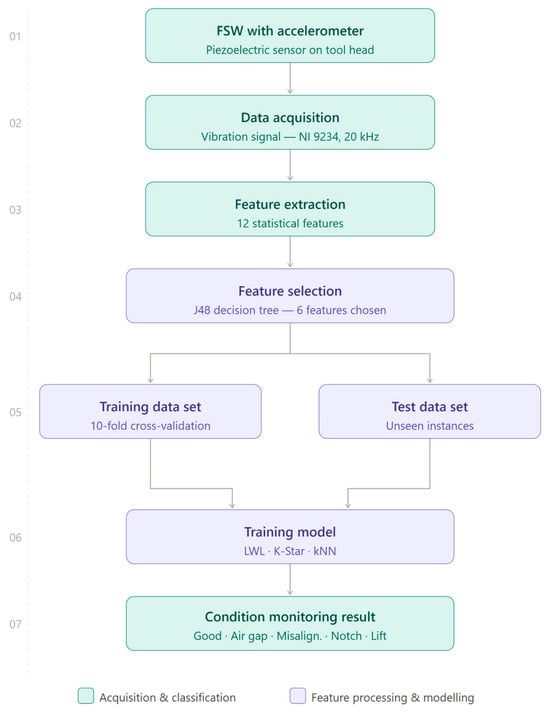
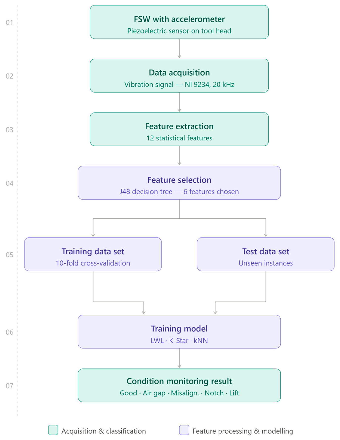
Although vibration-based FSW tool condition monitoring has been studied, the application of lazy learning algorithms to this problem has not been reported. The classification accuracy achieved with RF for the same FSW setup was 73.16% at 1400 rpm [20], which leaves room for improvement. The present study aims to improve classification accuracy by applying kNN, K*, and LWL classifiers to vibration signals acquired from a PLC-controlled FSW machine operating on Aluminium 5083 alloy at 1400 rpm. Statistical descriptors extracted from raw signals are refined through J48-based feature selection, and the three classifiers are systematically benchmarked to identify the best-performing option. The overall analytical workflow is illustrated in Figure 1.
Figure 1.
Proposed methodology for vibration-based fault detection and classification in friction stir welding.
2. Experimental Studies
The primary objective of this study was to determine whether the FSW tool was in a serviceable condition or had developed a fault, and, if faulty, to identify its type. The two initial stages test setup configuration and data collection procedure are detailed in the subsections that follow.
2.1. Experimental Setup
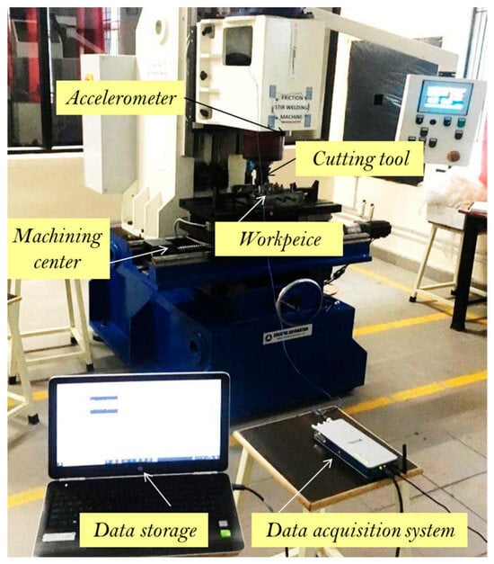
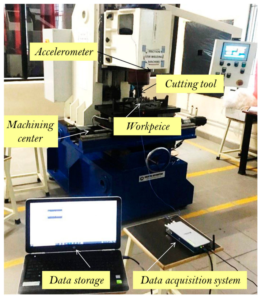
All experiments were conducted on a hydraulic, PLC-controlled FSW machine maintained in full working order (Figure 2). The technical parameters of the machine are listed in Table 1.
Figure 2.
Experimental setup FSW Machine.
Table 1.
Standard parameters of the FSW machine.
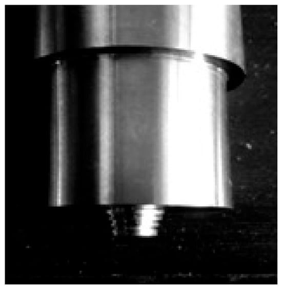
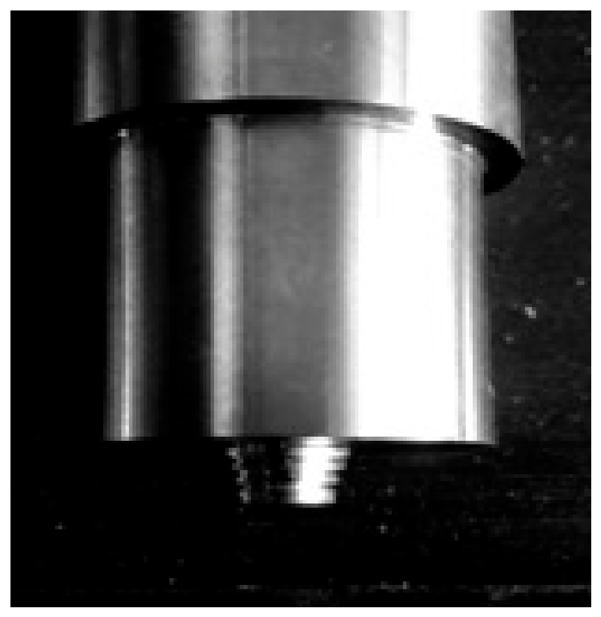
The Aluminium 5083 alloy grade which is widely used in marine and automotive applications was selected as workpiece [1]. Each plate was cut to 25 mm × 25 mm × 5 mm. The rotating tool comprised H13 hot-work tool steel, chosen for its combined thermal stability and abrasion resistance at process temperatures [24]. It had a threaded tappered pin profile and a pin depth of 5.75 mm (Figure 3). All joints were produced in a single welding pass at a fixed rotational speed of 1400 rpm and a traverse rate of 30 mm/min [25].
Figure 3.
FSW Tool with threaded pin.
Vibration data were captured using a piezoelectric accelerometer bonded adhesively to the tool head (Figure 4). Piezoelectric accelerometers are the standard transducer for condition monitoring applications because of their wide frequency range and their ability to detect small-amplitude vibrations without being damaged by the high-amplitude excitations that occur during normal machine operation. In this study, Dytran 3010A4 monoaxial piezoelectric accelerometer with a measurement range of ±500 g and a charge sensitivity of 10.26 mV/g was used for collecting the raw data. key technical specifications are as follows:
- Sensitivity: 10 mV/g.
- Measurement range: ±500 g.
- Frequency range: 2 Hz to 10 kHz (±3 dB).
- Resonant frequency: ≥70 kHz.
- Mounting: Stud mount, tool head perpendicular to workpiece surface.
- Connector type: 10–32 coaxial.
Figure 4.
Piezoelectric accelerometer.
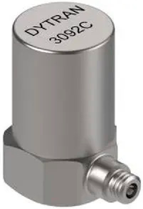
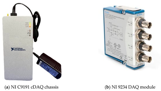
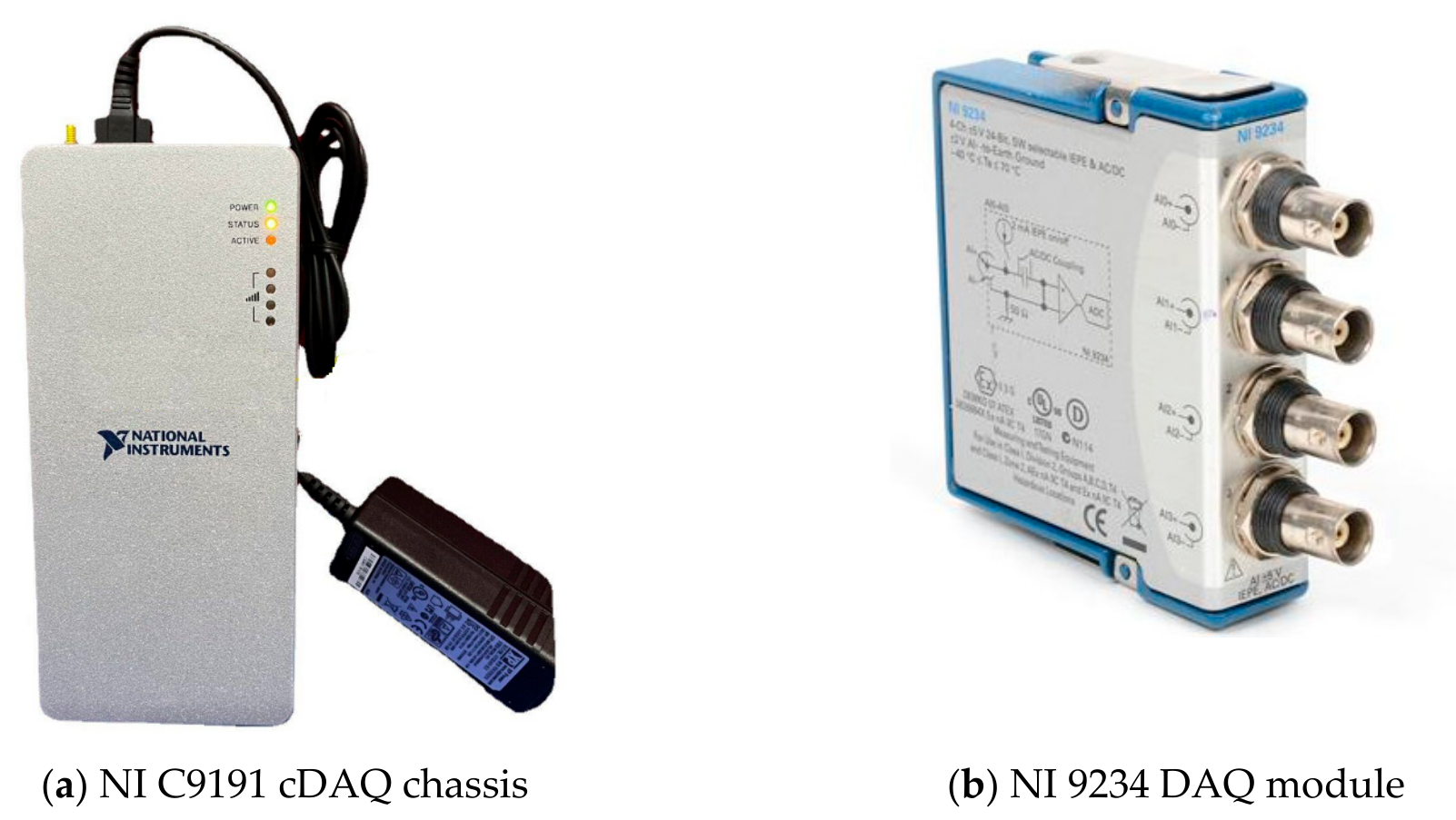
Accelerometer output was routed to a wireless four-channel data acquisition module (NI 9234, 51.2 kS/s) interfaced via an NI 9191 cDAQ chassis, as depicted in Figure 5a,b. This configuration was adopted from a prior FSW tool monitoring study that used the identical hardware setup [20]. The raw vibration signatures were captured using the NI LabVIEW programme.
Figure 5.
Data acquisition systems.
2.2. Experimental Procedure
Initially, the test rig was assumed to be in good condition, with all components brand new. Vibration signals were first recorded under the good condition and then under each fault condition, one at a time, while all other components remained unaltered. The signals were acquired with the following settings:
- Sample length: A sample length of 2048 (211) was chosen. If the number of samples is too small, the statistical measures computed from the signal become unreliable. If the number of samples is too large, computation time increases. To balance these two considerations, 2048 was selected as the sample length.
- Sampling frequency: Using the Nyquist sampling theorem, a sampling frequency of 20 kHz was selected.
- Number of samples: A minimum of 100 samples were collected for each of the five conditions.
The accelerometer was mounted vertically on the tool head (Figure 2). The monoaxial piezoelectric accelerometer (Model: Dytran 3010A4; Make: Dytran Instruments, Inc., Chatsworth, CA, USA) was mounted on the tool head with its sensing axis oriented perpendicular to the workpiece surface, aligned with the tool’s rotational axis (Z-axis), thereby primarily capturing axial vibrations. This mounting orientation was selected on the basis that the axial force is the dominant and most diagnostically sensitive mechanical parameter in FSW, as all process and setup fault conditions investigated in this study produce characteristic and distinguishable perturbations in the axial vibration signature. The accelerometer was secured to the tool head using a stud mount to ensure rigid coupling and to minimise signal attenuation across the frequency range of interest.
The 100 samples collected per operating condition were ensured to be statistically independent through the following measures. Each sample was acquired from a separate welding trial conducted under identical process parameter settings, ensuring that no two samples were derived from the same continuous signal record. The experimental setup, including workpiece fixturing and tool positioning, was fully reset between successive trials to eliminate any inter-sample dependency arising from residual thermal or mechanical effects. All samples were extracted exclusively from the steady-state phase of the welding signal, deliberately excluding the transient tool plunge and retract phases, which exhibit non-stationary behaviour and could otherwise introduce systematic bias into the feature extraction process. These precautions collectively ensure that the assembled dataset satisfies the independence assumption underlying the 10-fold cross-validation scheme adopted for classifier performance evaluation, thereby providing a statistically sound basis for the reported classification results.
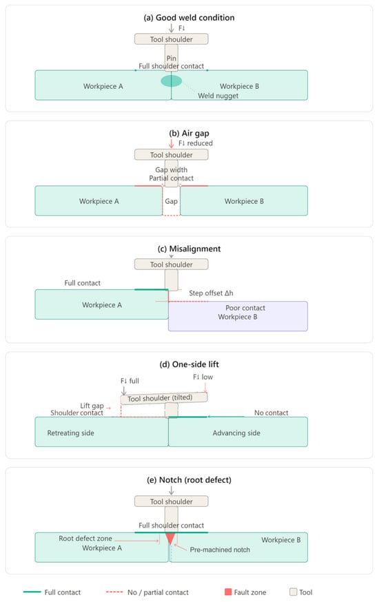
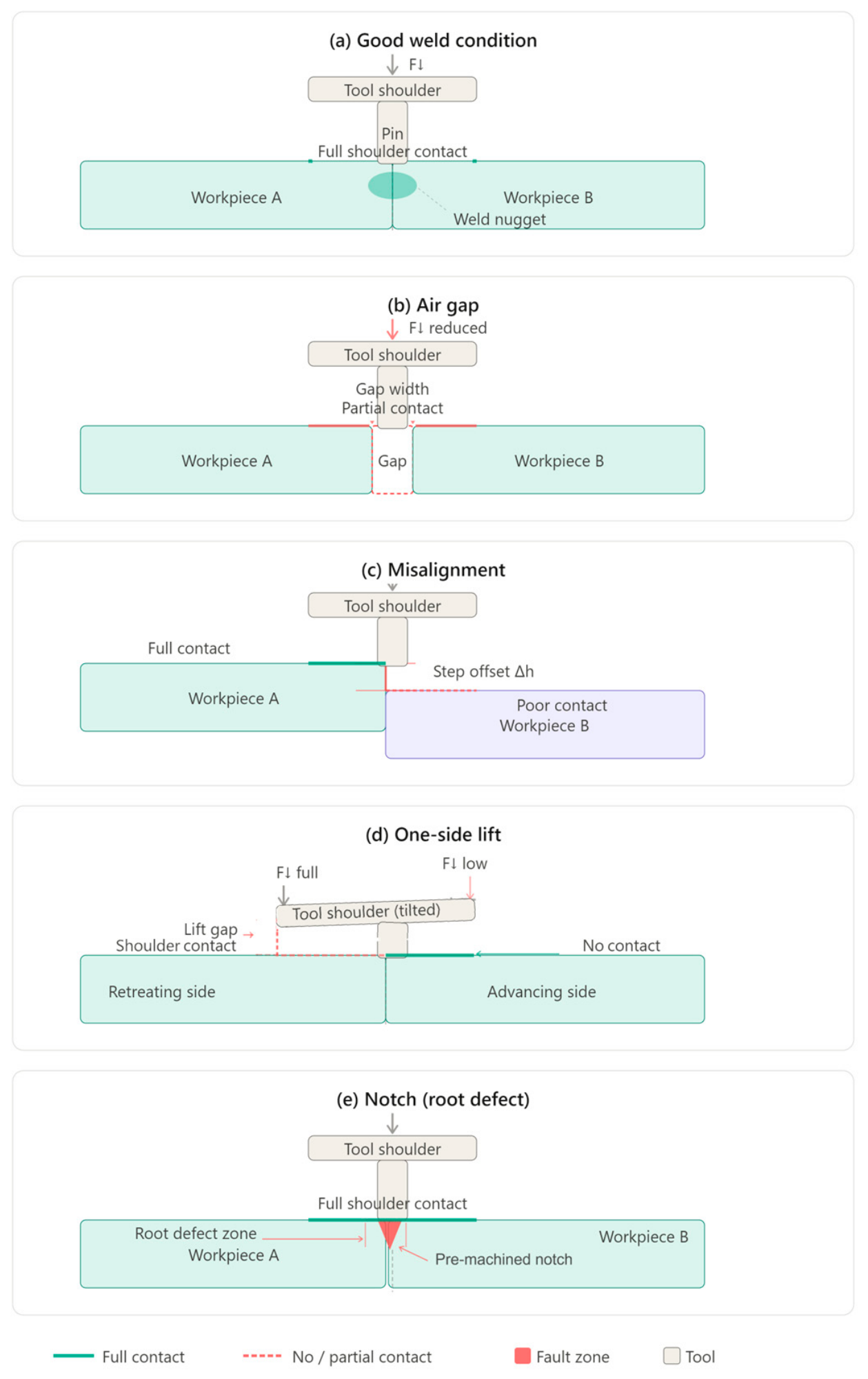
The following faults were simulated one at a time on the workpiece, while all other components remained in good condition. The corresponding vibration signals were acquired under each condition. Figure 6 shows the various fault conditions simulated in this study.
Figure 6.
Schematic cross-section representations of the five FSW process conditions investigated in this study: (a) good weld, (b) air gap, (c) misalignment, (d) one-side lift, and (e) notch.
- Good condition: The schematic depicts full and symmetric tool shoulder contact across both workpieces, with the weld nugget formed at the joint interface under a uniform downward forging force.
- Air gap: The schematic clearly shows the physical gap introduced between the two workpiece plates at the joint line, with the resulting reduction in shoulder contact area and downward force explicitly annotated.
- Misalignment: The schematic illustrates the deliberate vertical step offset (Δh) between the two abutting workpieces, highlighting the asymmetric shoulder contact—full on one side and poor on the other [26].
- One-side lift: The schematic represents the tilted tool shoulder with the resulting lift gap on the retreating side, asymmetric forging force distribution, and loss of shoulder contact on one side of the joint.
- Notch: The schematic depicts the pre-machined triangular notch introduced at the root of the joint interface, with the root defect zone clearly annotated to distinguish it from the shoulder contact region above.
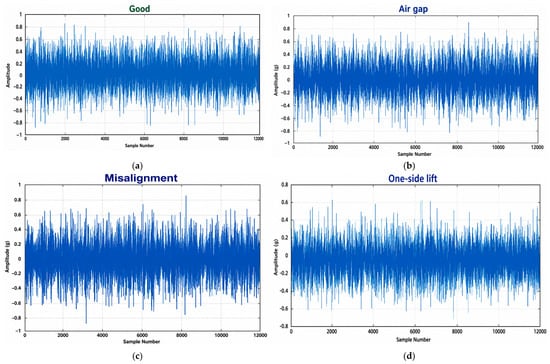
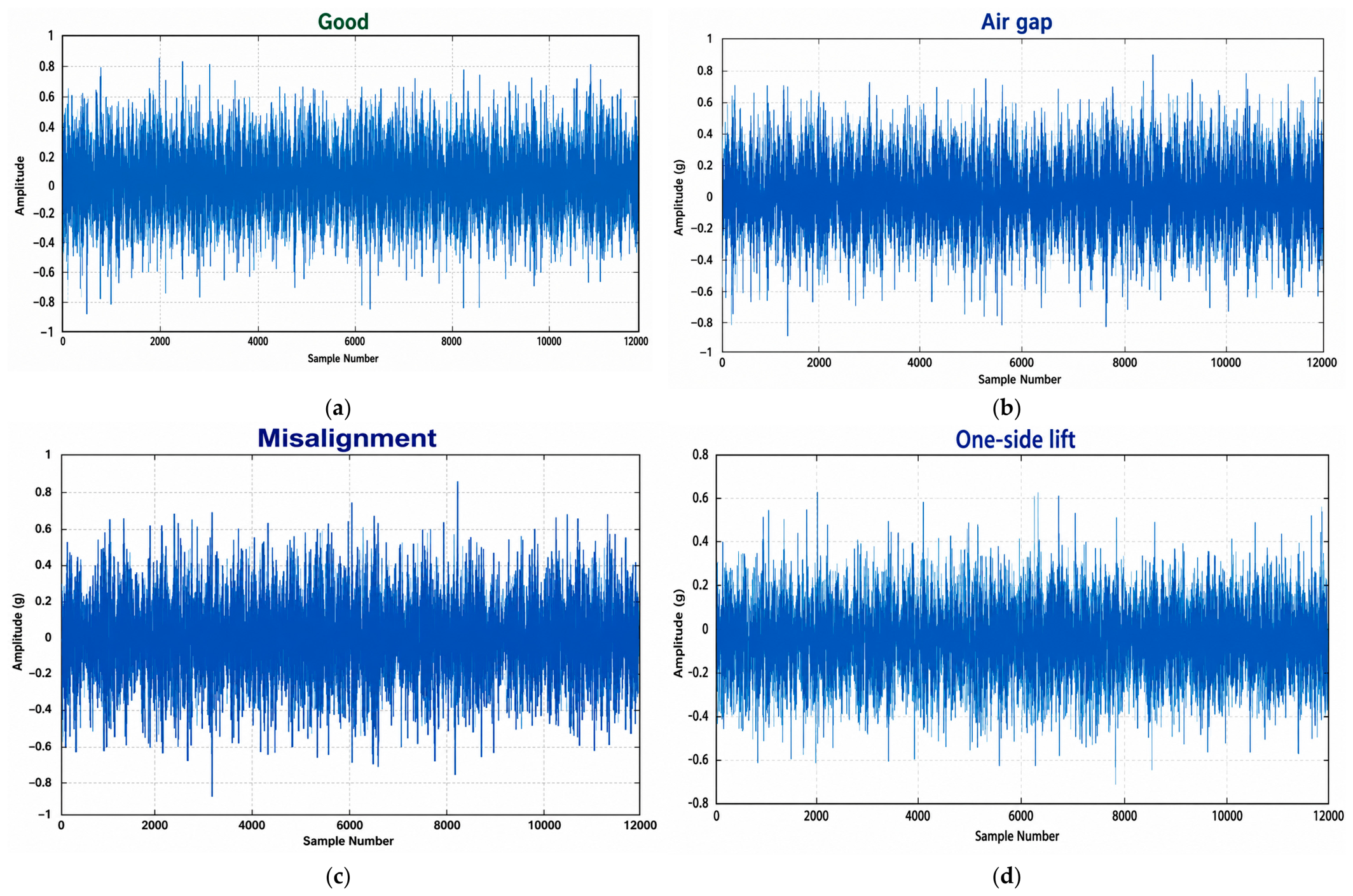
Figure 7a–d show the time-domain vibration signals recorded under the four fault conditions. From these plots, it can be seen that the magnitude of the acquired vibration signal varies with the type of fault simulated. These differences in signal characteristics form the basis for the feature extraction carried out in Section 3.
Figure 7.
Raw vibration signals acquired during FSW under different process conditions: (a) good weld, (b) air gap, (c) misalignment, and (d) one-side lift.
3. Feature Extraction
Feature extraction is the process of computing some measures which will represent the signal. Since the raw vibration signal cannot be used directly as input to a classifier, features must be extracted from it before classification is carried out. In this study, twelve statistical parameters were extracted from each signal sample. These features have been used widely in vibration-based fault diagnosis studies and carry sufficient discriminative information for classification tasks [13]. The features were computed using a LabVIEW graphical program. Not all twelve features may contribute equally to classification. Features that add little discriminative information increase computational cost without improving accuracy. Feature selection was therefore carried out to identify the most informative subset, as described in Section 4.
4. Feature Selection Using J48 Decision Tree Algorithm
Feature selection reduces the number of input variables passed to the classifier, lowers computation time, and often improves classification accuracy by removing features that add noise [27]. Among the available feature selection approaches, the J48 decision tree algorithm was adopted in the present study owing to its suitability for multi-class classification problems and its ability to evaluate the collective discriminative power of features rather than assessing each feature in isolation. Unlike conventional filter methods, which rank features based on statistical measures such as correlation or information gain without accounting for feature interdependencies, J48 inherently captures the conditional relationships between features during the tree construction process. This characteristic makes it effective in identifying a compact and non-redundant feature subset that retains the most diagnostically relevant information from the raw vibration signal. Furthermore, the tree-based structure of J48 offers a transparent and physically interpretable selection outcome, which is particularly valuable in engineering fault diagnosis applications where the traceability of selected features to their physical origin is important for result validation. The computational efficiency of J48 also makes it practical for datasets of the size encountered in this study, avoiding the high computational cost associated with population-based optimisation approaches such as genetic algorithms or particle swarm optimisation. On these grounds, J48 was preferred over alternative methods including principal component analysis, correlation-based feature selection, and evolutionary search strategies. J48 builds a tree by selecting, at each node, the attribute that gives the greatest reduction in entropy—a measure of class impurity [13]. This selection criterion is called information gain.
For a set of samples S, the entropy is defined as:
where Pi is the proportion of samples in S that belong to class i.
Entropy(S) = −Σ Pi log2 Pi
The information gain of an attribute A with respect to S is:
where Sv is the subset of S for which attribute A takes value v.
Gain(S, A) = Entropy(S) − Σ (|Sv|/|S|) × Entropy(Sv)
The attribute with maximum information gain is placed at the root; attributes appearing at the top levels of the tree are those that best separate the classes.
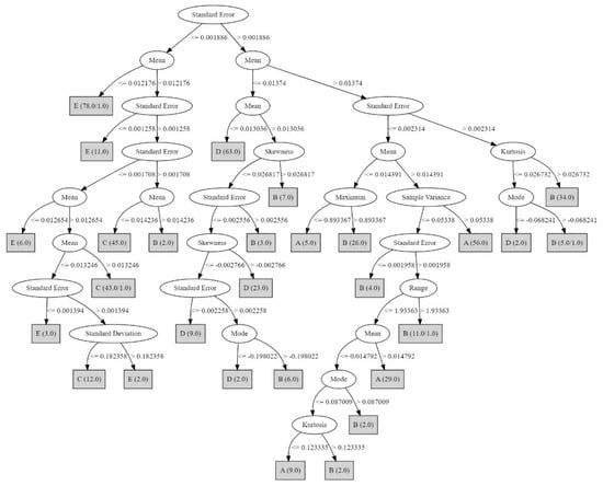
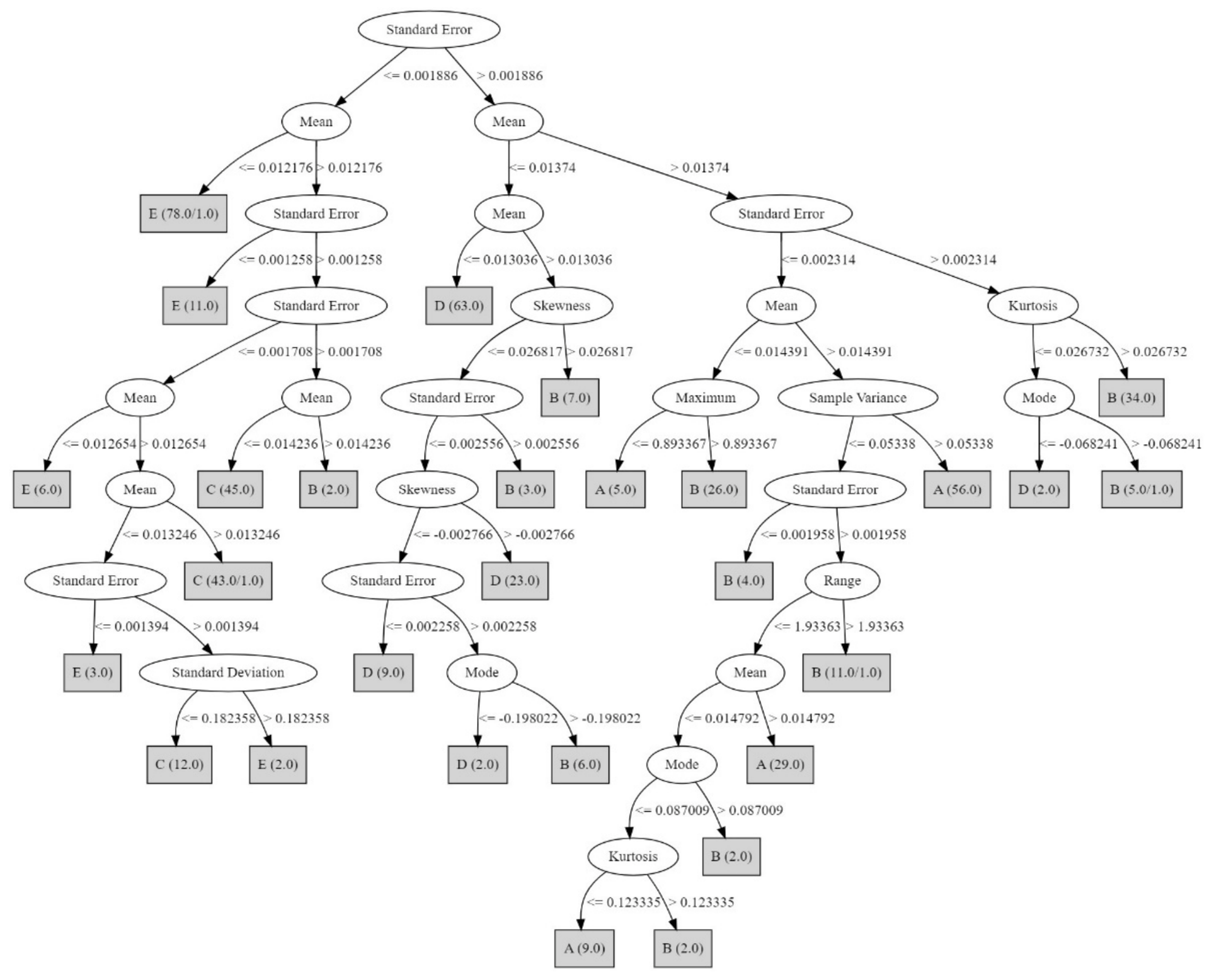
The decision tree was constructed using the twelve statistical features listed in Table 2 as input. The contribution of each feature in the tree is indicated by the numbers in parentheses at each leaf: the first number gives the count of correctly classified data points at that node, and the second (where present) gives the misclassified count. The features appearing at the top of the decision tree are the most important for classification [26]. The decision tree obtained is shown in Figure 8.
Table 2.
Statistical features extracted from vibration signals.
Figure 8.
Decision Tree Flowchart.
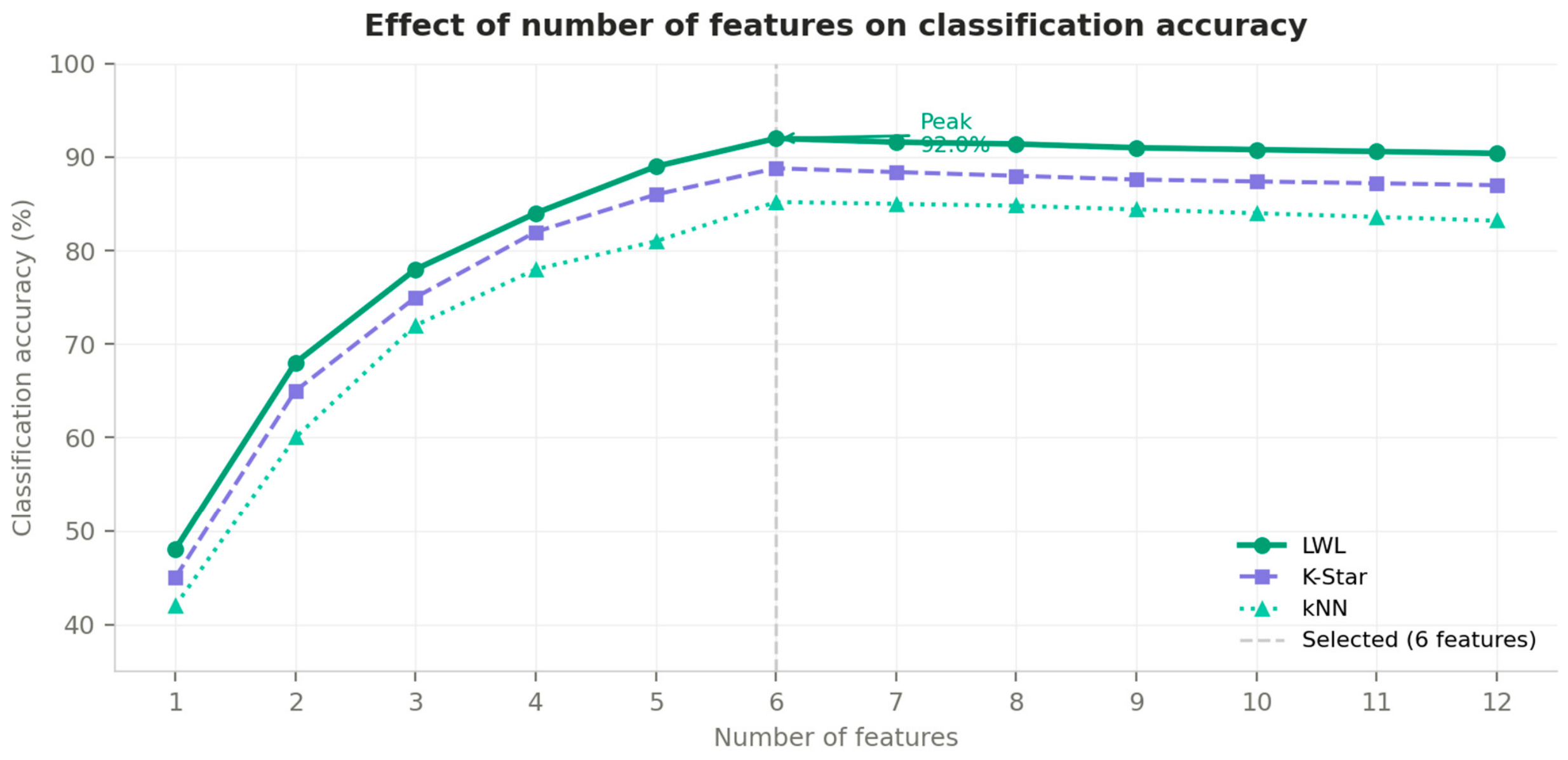
From the decision tree, six features were identified as the leading contributors to classification: Standard Error, Skewness, Mean, Kurtosis, Maximum, and Sample Variance. The remaining six features—Sum, Median, Mode, Minimum, Range, and Standard Deviation—appeared at lower levels of the tree or were absent altogether. These features were therefore excluded, as they contributed little to the classification of the fault conditions considered in this study. To verify this selection, the effect of the number of features on classification accuracy was studied.
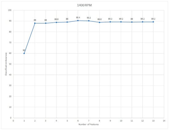
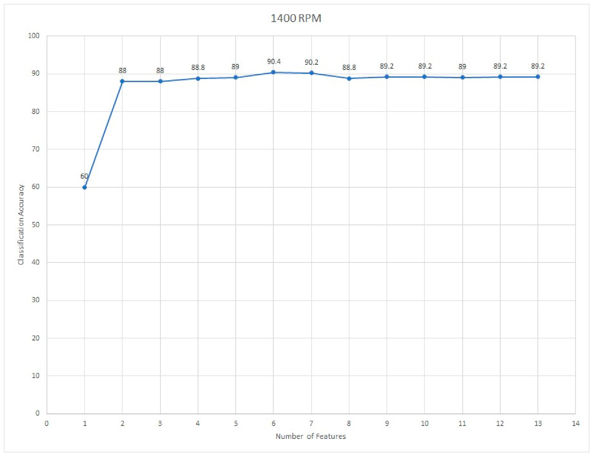
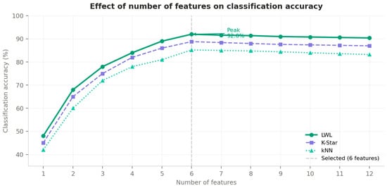
Starting from the highest-ranked feature, features were added one at a time and the classification accuracy was recorded after each addition. The results are plotted in Figure 9. Classification accuracy rises steadily up to six features and levels off thereafter, confirming that six is the effective number for this dataset. This approach for determining the optimal feature count has been followed in several earlier fault diagnosis studies [13]. The six selected features, Standard Error, Mean, Skewness, Kurtosis, Maximum, and Sample Variance were used as input to the three lazy learning classifiers described in Section 5.
Figure 9.
Effect of the number of features on classification accuracy using the J48 decision tree algorithm for feature selection.
5. Machine Learning Algorithms
The final processing stage involves training and testing three lazy classifiers on the six selected features from Section 4: Instance-Based kNN, K*, and LWL. Lazy learning algorithms do not construct a generalised model during training; instead, the training data is retained, and a local model is built only when a query instance is presented [21]. This deferred construction reduces the risk of overfitting and makes these classifiers naturally suited to datasets where the decision boundary is irregular or varies across the feature space, as is often the case with vibration signals from a machining process. All three classifiers were evaluated using 10-fold cross-validation.
5.1. Instance-Based kNN
Prior to classification, the six features selected by the J48 decision tree algorithm were subjected to min-max normalisation, independently applied to each feature to rescale all values to the range [0, 1]. This preprocessing step is particularly critical for the distance-sensitive classifiers employed in this study—specifically kNN and LWL—as features with larger absolute magnitudes would otherwise disproportionately dominate the inter-instance distance computation, introducing systematic bias into the neighbourhood identification and local model construction processes. Normalisation was performed within each fold of the 10-fold cross-validation scheme, with scaling parameters computed exclusively from the training partition and applied to the corresponding test partition, thereby ensuring that no information from the test fold influenced the normalisation process. This procedure safeguards the integrity and generalisability of the reported classification performance metrics.
The k-Nearest Neighbour (kNN) algorithm classifies a query instance by majority voting among its k closest training samples in the feature space [28]. The value of k determines the sensitivity of the classifier: a small k makes the model sensitive to noise, while a large k smooths the decision boundary but may dilute local patterns. In this study, k was set to 1, which is the default setting for this classifier. The distance between the query point and each training instance was measured using the Euclidean distance metric. Three distance weighting options were evaluated:
- No distance weighting: All neighbours are given equal importance, regardless of their distance from the query point.
- Inverse distance weighting (1/d): Nearer neighbours have a stronger influence on the outcome. This option gave the best result in the present study.
- Complement weighting (1 − d): Similar to inverse weighting but with a different scaling; nearer neighbours still dominate but the influence gradient is smoother.
The nearest neighbour search algorithm was also varied—options tested included linear search, KD-tree, ball tree, and cover tree. The combination of inverse distance weighting with a linear nearest neighbour search gave the best classification accuracy for this dataset and was adopted for the final.
5.2. K-Star (K*)
K-Star is an instance-based classifier that uses an entropy-based distance function rather than a geometric distance measure such as Euclidean distance [22]. The entropy-based measure accounts for the information content in the data, which makes it more effective than simple distance metrics when feature distributions are complex or overlapping. This is useful for vibration signals, where features extracted from different fault conditions can take similar numerical values.
K-Star handles missing attribute values through four modes:
- M1—Ignore missing cases: Data points with missing attribute values are excluded from the neighbourhood. This avoids misleading distance calculations but reduces the effective training set size.
- M2—Normalise over attributes: Features are normalised in instances with missing values so that the distance calculation remains consistent.
- M3—Treat missing as maximally distinctive: A missing value is treated as maximally different from all observed values. This is useful when absence of a measurement is itself informative.
- M4—Average column entropy curves: The contribution of a missing value is estimated from the average entropy of the column. This was the mode adopted in the present study and gave the best result.
Prior to classification, the integrity of the extracted feature dataset was verified, confirming that no missing values were present across all 500 samples and 12 statistical features. The complete and fully populated nature of the dataset is attributable to the controlled data acquisition protocol employed, wherein vibration signals were recorded continuously under stable welding conditions and features were extracted exclusively from the steady-state signal phase. The M4 missing value handling parameter reported in the default WEKA configuration for the K-Star classifier was therefore not invoked during the classification process, as the dataset required no imputation or missing value treatment. The global blend parameter, which controls the degree of randomness in the entropy-based distance, was varied between 1 and 100. A global blend of 30 produced the highest classification accuracy and was used for the final results. K-Star has been applied previously for tool condition monitoring by Painuli et al. [22] and for gear fault classification by Ravikumar et al. [23], both of which reported competitive classification accuracies, consistent with the performance observed in this study.
5.3. Locally Weighted Learning (LWL)
Locally Weighted Learning (LWL) is a non-parametric algorithm that builds a separate local model around each query point at prediction time, rather than fitting a single global model to the entire training set [21]. LWL assigns higher weights to training instances near each query point. The local model is then fitted using these weighted instances. Because the model is constructed fresh for each query, LWL adapts naturally to variations in the data distribution across the feature space. It requires no global model to be trained in advance, adapts to local variations in vibration patterns, and achieves results that match or exceed those of more complex algorithms such as the Probabilistic Neural Network [29].
It is acknowledged that the combination of LWL with Random Forest as the base learner represents a non-standard configuration that carries a higher per-query computational cost relative to conventional LWL implementations using simple base learners such as decision stumps or linear models. Since LWL constructs a locally weighted model at each query point and Random Forest itself involves training an ensemble of decision trees through bootstrap aggregation, the compounded inference latency of this combination may present practical constraints for deployment in high-speed real-time online monitoring systems. In the present study, this combination was evaluated within an offline cross-validation framework, where computational latency was not a primary constraint, and its inclusion was motivated by the improved classification robustness afforded by the ensemble base learner in locally weighted neighbourhoods. For real-time deployment, it is recommended that LWL be paired with computationally lighter base learners, or that the LWL–RF combination be implemented on dedicated embedded hardware or parallel computing platforms to meet the latency requirements of online FSW process monitoring. This aspect is identified as an important direction for future optimisation of the proposed framework.
In this study, RF was configured as the base learner within the LWL framework, with a linear neighbour search strategy. The kernel bandwidth parameter was set to zero, enabling automatic data-driven bandwidth determination. These settings were identified through parameter tuning and gave the best result. LWL has been used for vibration-based condition monitoring in an earlier study by Joshuva and Sugumaran [20], where it achieved a classification accuracy of 93.83% for wind turbine blade fault diagnosis and outperformed both kNN and K* in terms of accuracy and computation time. A similar trend was observed in the present study, where LWL produced the highest classification accuracy among the three classifiers, as reported in Section 6.
Table 3 summarize the key parameters used by the lazy classifiers namely LWL (Locally Weighted Learning), K-Star, and kNN (k-Nearest Neighbour). All three classification algorithms were implemented using the WEKA (Waikato Environment for Knowledge Analysis) machine learning workbench, version 3.8.6, developed by the University of Waikato, New Zealand. WEKA provides robust and well-validated built-in implementations of all three classifiers and was selected for this study due to its widespread adoption in condition monitoring and fault classification research, its transparent algorithm parameterisation, and its support for 10-fold cross-validation—which was employed in this study to ensure reliable and unbiased performance estimation.
Table 3.
Summary of the three lazy learning classifiers used in this study.
6. Results and Discussion
Vibration signals were acquired from the FSW machine under five tool conditions. A total of 500 samples (100 per condition) were collected. The six features selected by the J48 algorithm Standard Error, Mean, Skewness, Kurtosis, Maximum, and Sample Variance were used as inputs to all three classifiers. All classifiers were evaluated using 10-fold cross-validation [30].
6.1. Classification Using k-Nearest Neighbour (kNN)
The kNN classifier was configured with k = 1. The distance weighting method and nearest neighbour search algorithm were varied while all other parameters were held constant. The following results were obtained:
- Inverse distance weighting (1/d) with a linear NN search algorithm gave the highest accuracy among all parameter combinations tested.
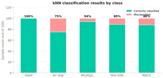
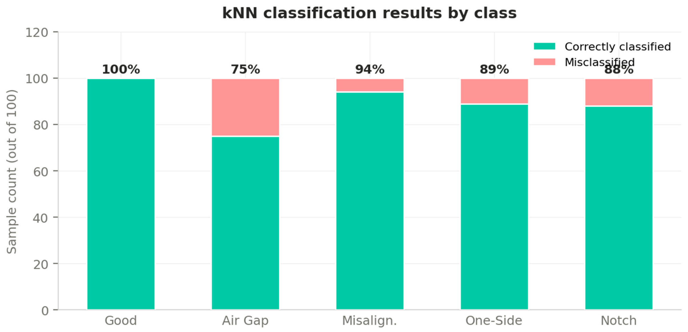
- The classifier correctly classified 426 out of 500 samples, giving a classification accuracy of 85.2%. The remaining 74 samples (14.8%) were misclassified.
- Most misclassifications occurred between the air gap condition and the one-side lift condition, which produce similar amplitude characteristics at 1400 rpm.
The distance weighting and nearest neighbour search settings were applied. Inverse distance weighting with linear NN search gave the best performance. The Figure 10 demonstrates the class wise accuracy with kNN classifier.
Figure 10.
Classification results of the kNN classifier (accuracy per class, 100 samples each).
6.2. Classification Using K-Star (K*)
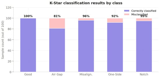
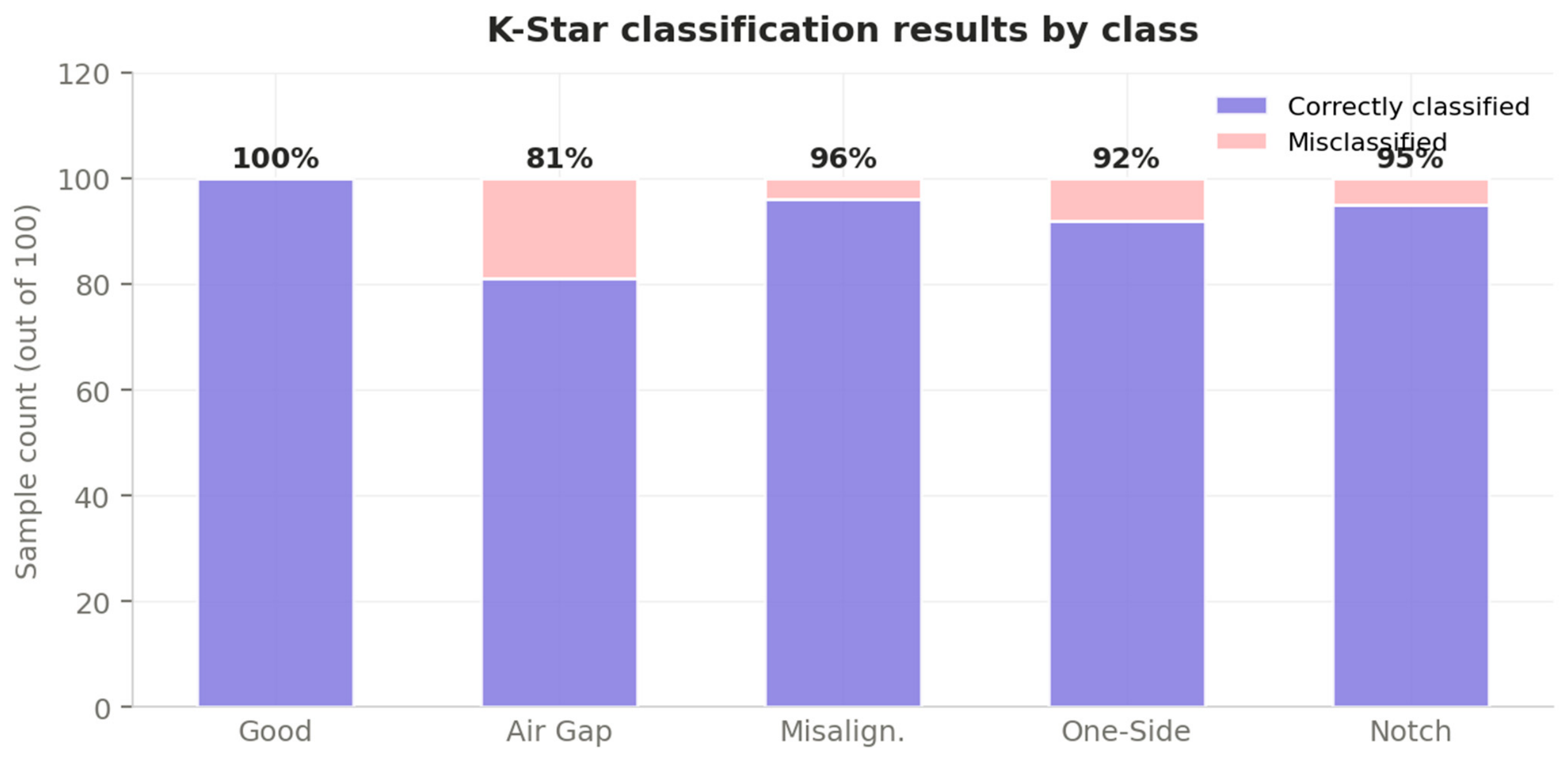
The K* classifier used entropy auto-blend set to true and missing attribute handling via the average column entropy curves mode (M4). The global blend parameter was varied from 1 to 100. Figure 11 shows the classification result of K*.
Figure 11.
Classification results of the K-Star classifier (accuracy per class, 100 samples each).
- A global blend of 30 gave the highest accuracy. The entropy-based distance measure proved more effective than Euclidean distance for this dataset, consistent with results reported by Painuli et al. [21] for tool condition monitoring.
- K-Star correctly classified 444 out of 500 samples, giving a classification accuracy of 88.8%. This is 3.6 percentage points higher than kNN.
- The air gap condition remained the most difficult class to identify correctly, with a TP rate of 0.810 and the highest FP rate of 0.035 among all classes.
6.3. Classification Using Locally Weighted Learning (LWL)
The LWL classifier used the RF as the base classifier and a linear NN search. The kernel bandwidth parameter was set to 0 (automatic). The results are reported below.
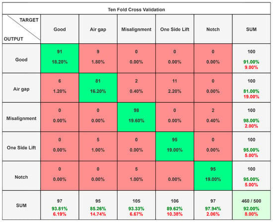
- LWL correctly classified 460 out of 500 samples, giving a classification accuracy of 92%. Only 40 samples (8%) were misclassified.
- The kappa statistic was 0.9, the MAE was 0.07, and the RMSE was 0.1649. The RAE was 17.39% and the RRSE was 41.8% (Refer Table 4).Table 4. Overall classification accuracy of the LWL classifier.
- Except airgap, none of the good-condition samples were misclassified as faulty, and none of the faulty samples were classified as good (except airgap).
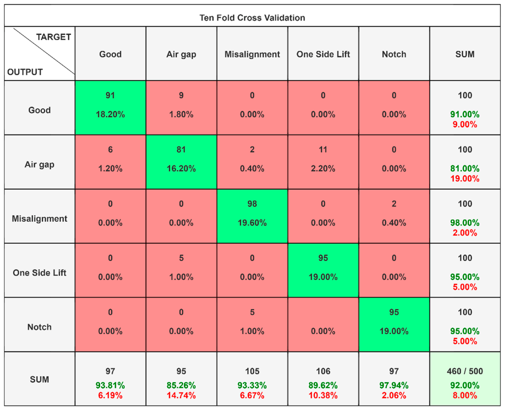
- Figure 12 shows the confusion matrix which shows the overall classification accuracy of FSW tool with LWL classifier.Figure 12. Confusion Matrix of LWL Classifiers.
- The misalignment condition gave the highest TP rate of 0.980. Lateral tool deviation produces a distinctive increase in lateral vibration force, which the Maximum and Sample Variance features capture effectively.
- The air gap condition recorded the lowest TP rate of 0.810 and the highest FP rate of 0.035 (Figure 14). Loss of shoulder contact reduces vibration amplitude in a way that partially resembles the one-side lift condition at this spindle speed.
- The notch condition gave a TP rate of 0.950 and the highest precision of 0.979 among all five classes. The groove machined into the workpiece surface produces a spiky vibration component, which the Kurtosis feature—one of the six selected features—specifically measures.
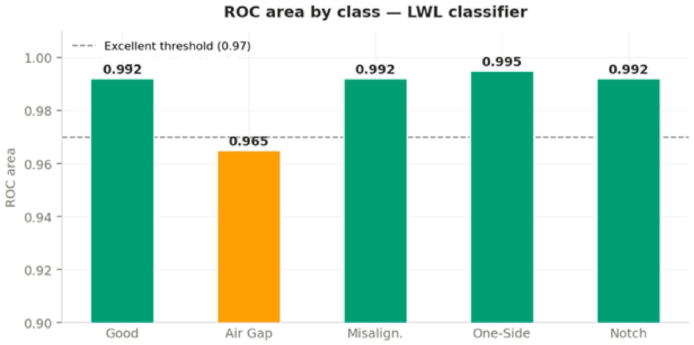
- All five classes achieved an ROC area above 0.96, with four classes exceeding 0.99 (Refer Figure 15). A ROC area above 0.97 is considered excellent for a multi-class fault diagnosis problem [28].
- The F-measure ranged from 0.831 for the air gap condition to 0.964 for the notch condition. This indicates that the classifier maintains a good balance between precision and recall across all five classes.
Table 5.
Class-wise accuracy of the LWL classifier.
Figure 13.
Class-wise TP rate, precision, and F-measure for the LWL classifier.
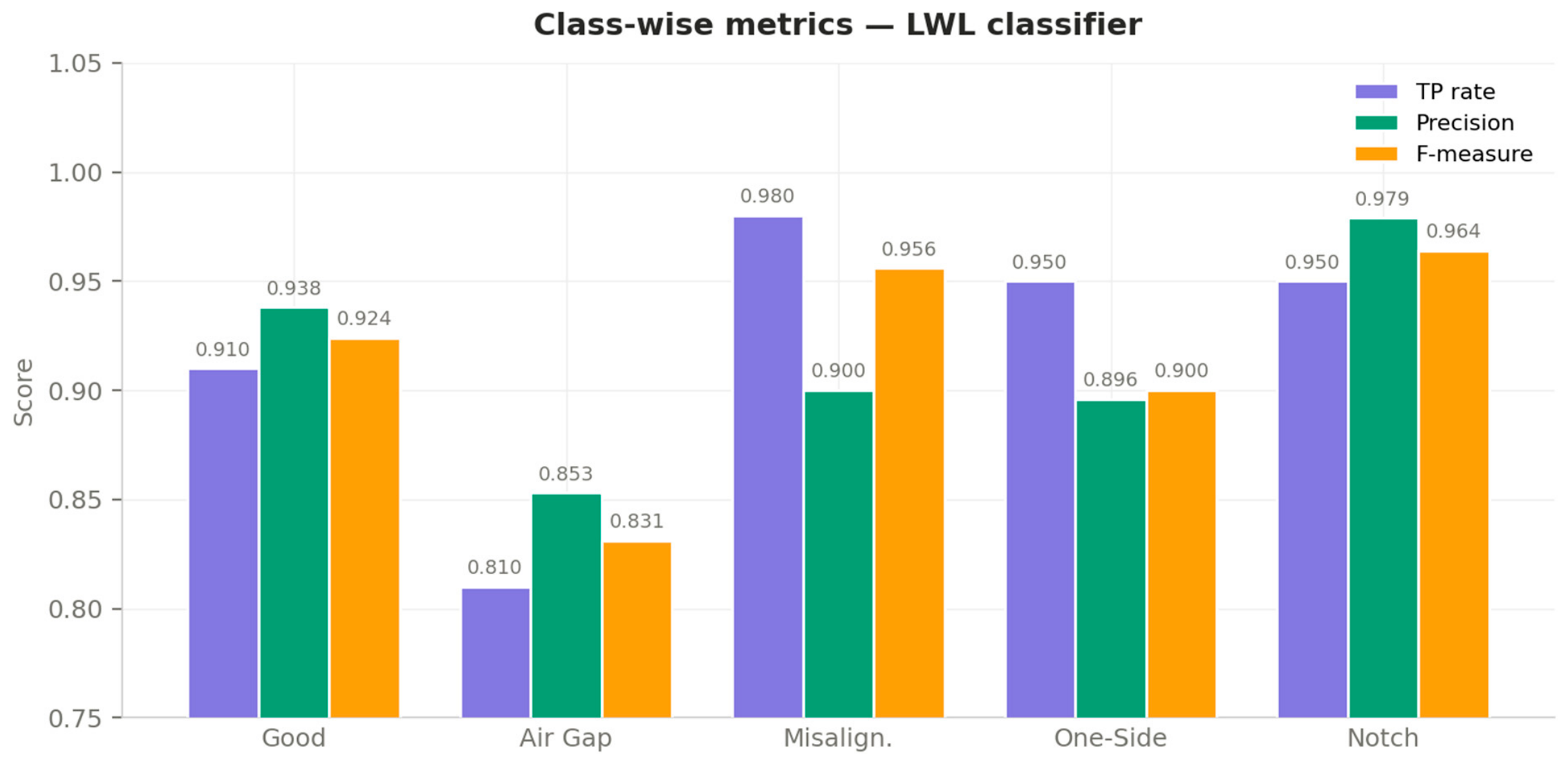
Figure 14.
False positive rate per class for the LWL classifier.
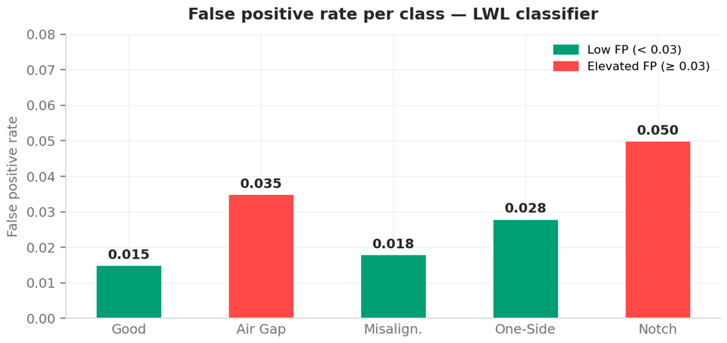
Figure 15.
ROC area per class for the LWL classifier.
The relatively lower classification accuracy of 81% observed for the air gap condition is attributed to the intermittent and amplitude-modulated nature of its vibration signature, which arises from the periodic bridging of the joint gap by the rotating tool pin during welding. This transient contact behaviour produces statistical feature values that partially overlap with those of the one-side lift condition—wherein asymmetric shoulder contact similarly results in a partial reduction in axial force and vibration amplitude—thereby increasing the inter-class confusion between these two fault categories. Furthermore, minor intra-class variability in the gap width across experimental trials introduces additional spread in the statistical feature distributions for the air gap class, reducing its separability in the feature space. Future work will investigate the use of time-frequency domain features and deep learning-based classification approaches to improve the discrimination of the air gap condition from other partial-contact fault classes.
6.4. Comparative Study
The classification accuracies of the three lazy learning classifiers are compared in Table 6 alongside the earlier Random Forest result [18]. The following observations are made.
Table 6.
Classification accuracies of kNN, K-Star, LWL and Random forest.
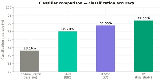
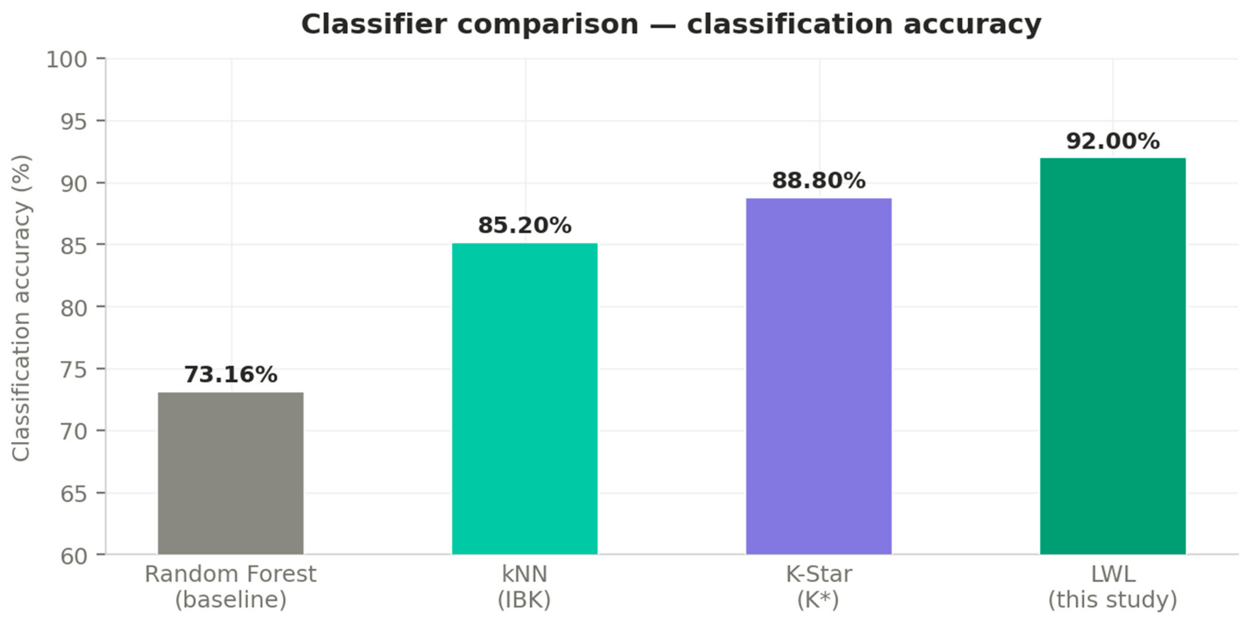
- Referring to Figure 16 and Table 6, LWL gave the highest classification accuracy of 92%, which is an improvement of 18.84 percentage points over the RF result reported in [18] for the same experimental setup. This improvement is attributed to the local weighting approach of LWL, where training instances closer to the query point have a greater influence on the classification decision. This is particularly effective for vibration data, where the decision boundary between fault conditions is not uniform across the feature space.Figure 16. Comparison of classification accuracy across all classifiers.
- The order of classification accuracy (LWL, K*, kNN) was the same for all feature counts from 1 to 12, as shown in Figure 17. Joshuva and Sugumaran [20] reported the same ordering for wind turbine blade fault diagnosis using vibration signals, which indicates that this trend holds across different vibration-based condition monitoring applications.Figure 17. Effect of the number of selected features on classification accuracy for the LWL, K-Star and kNN classifiers.
- K* outperformed kNN by 3.6 percentage points. The entropy-based distance in K* accounts for the information structure of the feature space, not just geometric proximity, which is beneficial for non-Gaussian vibration features such as Kurtosis and Skewness [21].
- The air gap condition was the hardest to classify correctly for all three methods. At 1400 rpm, the loss of shoulder contact produces only a moderate change in overall vibration level, creating partial overlap with the one-side lift condition in the feature space.
6.5. Future Research Direction
Wavelet and frequency-domain features may be used for improved air gap classification. Short-time Fourier transform and discrete wavelet transform features in the 1–5 kHz band are expected to resolve the overlap that time-domain statistical features cannot distinguish.
All experiments in this study were conducted at a spindle speed of 1400 rpm and a feed rate of 30 mm/min. The effect of spindle speed on classification accuracy has not been studied here. A study covering a range of speeds from 800 rpm to 2000 rpm and different feed rates would help determine whether a single trained model is sufficient across operating conditions or whether separate models are needed for each speed.
Fault conditions such as incomplete root fusion, flash formation, and tool breakage were not considered in this study. Including these conditions in the dataset would make the model more useful for practical FSW monitoring applications.
All experiments used Aluminium 5083 alloy as the workpiece material. Whether the trained model works for other materials such as copper alloys or magnesium alloys has not been verified. Investigating this would extend the scope of the approach to a wider range of FSW applications.
In this study, LWL, K*, and kNN each produced different misclassification patterns. A majority-vote ensemble of these three classifiers could potentially reduce the overall error rate below 8%, particularly for the air gap condition, which was the hardest class to classify correctly.
The tool condition changes progressively over a welding campaign. In this study, the classifier was trained once using a fixed dataset. An online learning variant of LWL that adds new instances to the training set as the tool degrades would allow the model to follow the change in tool condition without the need to retrain the classifier from scratch. This would make the system more practical for continuous monitoring over the full service life of the tool.
7. Conclusions
This study examined the condition monitoring of FSW tools through vibration analysis. Experiments were conducted on a PLC-controlled FSW machine at 1400 rpm using Aluminium 5083 alloy as the workpiece material. Vibration signals were recorded under five conditions good, air gap, misalignment, one-side lift, and notch with 100 samples per condition. Twelve statistical features were extracted and reduced to six using the J48 decision tree. Three lazy learning classifiers kNN, K*, and LWL were trained and evaluated using 10-fold cross-validation. Compared to all considered algorithm, LWL gave the highest classification accuracy of 92%, followed by K-Star at 88.8% and kNN at 85.2%. Among the five fault conditions, misalignment was the easiest to identify (TP rate = 0.980) and air gap was the most difficult (TP rate = 0.810). The confusion between air gap and one-side lift at this spindle speed points to the need for frequency-domain features in future work. The kappa statistic of 0.900, an ROC area above 0.965 for all classes, and an F-measure above 0.831 for all classes together confirm that LWL produces reliable, well-balanced classifications across the full set of fault conditions. Hence, LWL is recommended as the classifier for real-time FSW tool condition monitoring at 1400 rpm.
Author Contributions
Conceptualization, B.K.; methodology, B.K.; software, B.K.; validation, J.R.; formal analysis, J.R.; investigation, J.R.; resources, J.R.; data curation, L.P.J.; writing—original draft preparation, J.R.; writing—review and editing, S.G.; visualization, M.T.; supervision, J.R.; project administration, J.R.; funding acquisition, J.R. All authors have read and agreed to the published version of the manuscript.
Funding
This research received no external funding.
Data Availability Statement
Data will be made available upon request.
Acknowledgments
Authors acknowledge Alamelu Manghai for her support in data acquisition.
Conflicts of Interest
The authors declare no conflicts of interest.
References
- Mishra, R.S.; Ma, Z.Y. Friction stir welding and processing. Mater. Sci. Eng. R Rep. 2005, 50, 1–78. [Google Scholar] [CrossRef] [Scilit]
- Gibson, B.T.; Lammlein, D.H.; Prater, T.J.; Longhurst, W.R.; Cox, C.D.; Ballun, M.C.; Dharmaraj, K.J.; Cook, G.E.; Strauss, A.M. Friction stir welding: Process, automation, and control. J. Manuf. Process. 2014, 16, 56–73. [Google Scholar] [CrossRef] [Scilit]
- Squillace, A.; De Fenzo, A.; Giorleo, G.; Bellucci, F. A comparison between FSW and TIG welding techniques: Modifications of microstructure and pitting corrosion resistance in AA 2024-T3 butt joints. J. Mater. Process. Technol. 2004, 152, 97–105. [Google Scholar] [CrossRef] [Scilit]
- Thomas, W.M.; Nicholas, E.D. Friction stir welding for the transportation industries. Mater. Des. 1997, 18, 269–273. [Google Scholar] [CrossRef] [Scilit]
- Eren, B.; Guvenc, M.A.; Mistikoglu, S. Artificial intelligence applications for friction stir welding: A review. Met. Mater. Int. 2021, 27, 384–401. [Google Scholar] [CrossRef] [Scilit]
- Bird, C.R. Ultrasonic phased array inspection technology for the evaluation of friction stir welds. Insight Non-Destr. Test. Cond. Monit. 2004, 46, 31–36. [Google Scholar] [CrossRef] [Scilit]
- Bagavathiappan, S.; Lahiri, B.B.; Saravanan, T.; Philip, J.; Jayakumar, T. Infrared thermography for condition monitoring—A review. Infrared Phys. Technol. 2013, 60, 35–55. [Google Scholar] [CrossRef] [Scilit]
- Mezyk, J.; Kowieski, S. Monitoring the FSW processes with use of thermal imaging. Solid State Phenom. 2015, 220–221, 859–863. [Google Scholar] [CrossRef] [Scilit]
- Soundararajan, V.; Atharifar, H.; Kovacevic, R. Monitoring and processing the acoustic emission signals from the friction-stir-welding process. Proc. Inst. Mech. Eng. B J. Eng. Manuf. 2006, 220, 1673–1685. [Google Scholar] [CrossRef] [Scilit]
- Hassan, I.U.; Panduru, K.; Walsh, J. An In-Depth Study of Vibration Sensors for Condition Monitoring. Sensors 2024, 24, 740. [Google Scholar] [CrossRef] [Scilit] [PubMed]
- Tiboni, M.; Remino, C.; Bussola, R.; Amici, C. A review on vibration-based condition monitoring of rotating machinery. Appl. Sci. 2022, 12, 972. [Google Scholar] [CrossRef] [Scilit]
- Almutairi, K.M.; Sinha, J.K. Experimental vibration data in fault diagnosis: A machine learning approach to robust classification of rotor and bearing defects in rotating machines. Machines 2023, 11, 943. [Google Scholar] [CrossRef] [Scilit]
- Jegadeeshwaran, R.; Sugumaran, V. Comparative study of decision tree classifier and best first tree classifier for fault diagnosis of automobile hydraulic brake system using statistical features. Measurement 2013, 46, 3247–3260. [Google Scholar] [CrossRef] [Scilit]
- Altaf, M.; Akram, T.; Khan, M.A.; Iqbal, M.; Ch, M.M.I.; Hsu, C.-H. A new statistical features-based approach for bearing fault diagnosis using vibration signals. Sensors 2022, 22, 2012. [Google Scholar] [CrossRef] [Scilit] [PubMed]
- Chen, Q.; Nicholson, G.; Ye, J.; Roberts, C. Fault diagnosis using discrete wavelet transform (DWT) and artificial neural network (ANN) for a railway switch. In Proceedings of the Prognostics and Health Management Conference (PHM-Besançon), Besançon, France, 4–7 May 2020; pp. 67–71. [Google Scholar] [CrossRef] [Scilit]
- Madhusudana, C.K.; Kumar, H.; Narendranath, S. Condition monitoring of face milling tool using K-star algorithm and histogram features of vibration signal. Eng. Sci. Technol. Int. J. 2016, 19, 1543–1551. [Google Scholar] [CrossRef] [Scilit]
- Sánchez, R.-V.; Macancela, J.C.; Ortega, L.-R.; Cabrera, D.; García Márquez, F.P.; Cerrada, M. Evaluation of hand-crafted feature extraction for fault diagnosis in rotating machinery: A survey. Sensors 2024, 24, 5400. [Google Scholar] [CrossRef] [Scilit]
- Jegadeeshwaran, R.; Sugumaran, V. Fault diagnosis of automobile hydraulic brake system using statistical features and support vector machines. Mech. Syst. Signal Process. 2015, 52–53, 436–446. [Google Scholar] [CrossRef] [Scilit]
- Wang, Q.-A.; Lu, A.-W.; Ni, Y.-Q.; Wang, J.-F.; Ma, Z.-G. Bayesian network in structural health monitoring: Theoretical background and applications review. Sensors 2025, 25, 3577. [Google Scholar] [CrossRef] [Scilit] [PubMed]
- Balachandar, K.; Jegadeeshwaran, R. Friction stir welding tool condition monitoring using vibration signals and random forest algorithm—A machine learning approach. Mater. Today Proc. 2021, 46, 1174–1180. [Google Scholar] [CrossRef] [Scilit]
- Joshuva, A.; Sugumaran, V. A lazy learning approach for condition monitoring of wind turbine blade using vibration signals and histogram features. Measurement 2020, 152, 107295. [Google Scholar] [CrossRef] [Scilit]
- Painuli, S.; Elangovan, M.; Sugumaran, V. Tool condition monitoring using K-star algorithm. Expert Syst. Appl. 2014, 41, 2638–2643. [Google Scholar] [CrossRef] [Scilit]
- Ravikumar, K.N.; Madhusudana, C.K.; Kumar, H.; Gangadharan, K.V. Classification of gear faults in internal combustion engine gearbox using discrete wavelet transform features and K-star algorithm. Eng. Sci. Technol. Int. J. 2022, 30, 101048. [Google Scholar] [CrossRef] [Scilit]
- Alkhafaji, A.; Camas, D.; Lopez-Crespo, P.; Al-Asadi, H. The Influence of Tool Geometry on the Mechanical Properties and the Microstructure of AA6061-T6 Aluminum Alloy Friction Stir Spot Welding. Materials 2023, 16, 4135. [Google Scholar] [CrossRef] [Scilit] [PubMed]
- Buffa, G.; Campanile, G.; Fratini, L.; Prisco, A. Friction stir welding of lap joints: Influence of process parameters on the metallurgical and mechanical properties. Mater. Sci. Eng. A 2009, 519, 19–26. [Google Scholar] [CrossRef] [Scilit]
- Franke, D.; Rudraraju, S.; Zinn, M.; Pfefferkorn, F.E. Understanding process force transients with application towards defect detection during friction stir welding of aluminum alloys. J. Manuf. Process. 2020, 54, 251–261. [Google Scholar] [CrossRef] [Scilit]
- Indira, V.; Vasanthakumari, R.; Jegadeeshwaran, R.; Sugumaran, V. Determination of minimum sample size for fault diagnosis of automobile hydraulic brake system using power analysis. Eng. Sci. Technol. Int. J. 2015, 18, 59–69. [Google Scholar] [CrossRef] [Scilit]
- Altman, N.S. An introduction to kernel and nearest-neighbor nonparametric regression. Am. Stat. 1992, 46, 175–185. [Google Scholar] [CrossRef] [Scilit]
- Krishnamurthy, B.; Rakkiyannan, J. Enhancing tool condition monitoring in friction stir welding with probabilistic neural network algorithm. Front. Mech. Eng. 2025, 11, 1613216. [Google Scholar] [CrossRef] [Scilit]
- Kohavi, R. A study of cross-validation and bootstrap for accuracy estimation and model selection. In Proceedings of the International Joint Conference on Artificial Intelligence (IJCAI); Morgan Kaufmann: San Francisco, CA, USA, 1995; Volume 2, pp. 1137–1143. [Google Scholar]

Disclaimer/Publisher’s Note: The statements, opinions and data contained in all publications are solely those of the individual author(s) and contributor(s) and not of MDPI and/or the editor(s). MDPI and/or the editor(s) disclaim responsibility for any injury to people or property resulting from any ideas, methods, instructions or products referred to in the content. |
© 2026 by the authors. Licensee MDPI, Basel, Switzerland. This article is an open access article distributed under the terms and conditions of the Creative Commons Attribution (CC BY) license.