


Abstract
The intelligent detection of surface damage is crucial for ensuring safe and stable equipment operation. This study addressed the low efficiency, strong subjectivity, and inadequate representation capabilities of traditional single-feature-based damage identification methods by proposing an intelligent equipment surface damage classification method employing multi-feature fusion. The innovations of this method comprise the construction of a seven-dimensional model integrating brightness, texture, frequency domain, edge, and morphological features to comprehensively characterize the visual characteristics of six typical types of damage (fine crazing, inclusions, patches, pitted surfaces, rolled-in oxide scale, and scratches) and the application of a Bayesian probabilistic classification model based on adaptive kernel density estimation to identify damage type and determine the associated confidence. Experimental results obtained using a self-assembled dataset comprising 1619 training samples and 180 test samples indicated that the proposed method achieved a comprehensive accuracy of 97.77%, significantly outperforming traditional deep neural networks and Ant Forest algorithms. Thus, the proposed method provides an effective solution for the intelligent and efficient detection of equipment surface damage.
1. Introduction
Steel (including alloy and special steels) is the primary base material for a variety of military equipment, such as armor, bridges, ammunition, and artillery [1]. Ongoing equipment service causes the surfaces of these materials to develop defects, such as fine crazing, inclusions, patches, pitting, rolled-in oxide scale, and scratches, under the influence of multiple factors, including environmental exposure, applied load, and material aging. These defects not only damage the material surface but can also degrade material performance, seriously compromising the quality and performance of equipment [2,3,4]. Therefore, efficient and accurate surface damage detection technologies must be developed.
Surface detection methods have gradually advanced from strictly manual detection [5] to employing automated intelligent detection [6]. In the early stages of development, automated surface defect detection primarily relied on conventional image processing methods, such as edge detection based on the Canny operator [7] and threshold segmentation based on the Otsu algorithm [8]. These methods are not computationally complex and can achieve a certain degree of damage detection in simple scenarios; however, their detection performance heavily depends on low-level handcrafted intensity and gradient features, which are susceptible to interference in complex industrial environments, such as uneven illumination, surface oil contamination, and highly reflective surfaces, leading to false or discontinuous edge extraction and reduced identification accuracy [9]. Digital holography, as a non-contact optical measurement method, can image material surface cracks by recording holograms of acoustic wave propagation [10]. The development of deep learning technology has led to the widespread application of object detection networks, such as the Faster Region-based Convolutional Neural Network [11] and Mask Region-based Convolutional Neural Network [12], to identify surface damage. These methods can achieve detection accuracies exceeding 90% [13], but they are subject to obvious limitations, such as insufficient sample quantity, uneven sample distribution, overly simple classification tasks, and poor real-time performance [14,15,16], as well as high demand for computing resources and poor model interpretability, that prevent them from meeting the requirements for traceable detection results in industrial and military applications. To alleviate these issues, some studies have combined lateral shearing digital holographic microscopy with microscopic fringe projection profilometry and used convolutional neural networks for defect classification, achieving 99% accuracy on printed circuit board inspection [17]. Although this method still relies on deep learning, the hybrid optical sensor reduces computational burden.
In the field of composite materials and structural health monitoring, deep learning-based damage detection techniques have also advanced rapidly. For example, convolutional neural networks combined with infrared thermography can automatically identify impact damage in composite laminates, and ultrasonic guided waves with domain-adaptive transfer learning enable reliable structural damage assessment under varying operational conditions [18,19]. However, such data-driven methods generally rely on large-scale high-quality labeled data and high-performance computing resources, posing deployment challenges in scenarios with limited data access and high interpretability requirements, such as military equipment.
In recent years, damage detection technologies based on image processing have been widely used in industrial applications owing to their high efficiency and non-contact functionality. However, many conventional image processing methods rely on the extraction of a single feature and exhibit poor adaptability to multiple types and scales of damage [20]. The use of multi-feature fusion technology can improve defect detection accuracy in complex scenarios by integrating information from different dimensions [21] and has been successfully applied in fields such as medical image analysis [22] and wind turbine blade defect detection [23] accordingly. Indeed, recent research trends indicate that multi-feature fusion can effectively improve the recognition of small targets, complex textures, and multiple defect types in images. For example, Liu et al. [24] proposed a multi-scale feature fusion method for rainy-track image restoration, and Cui et al. [25] realized ship detection in synthetic-aperture radar images using multi-scale feature enhancement, demonstrating its advantages in complex scenarios. In addition, fringe projection profilometry based on a stereomicroscope can obtain three-dimensional surface topography at micrometer-level accuracy, offering a new approach for quantitative detection of tiny damage [26]. Particularly, for workpieces with complex surface textures (such as rusted or coated steel), a recently proposed FFT-guided morphological component analysis single-shot fringe projection technique can effectively separate texture and fringe signals, achieving high-precision 3D reconstruction without pre-calibration [27].
Furthermore, to address the problems of difficult sample acquisition and high labeling cost for surface damage, data augmentation strategies based on synthetic data have drawn widespread attention. For instance, generative adversarial networks can generate crack images with diverse morphologies to augment training sets and improve model generalization [28]; finite element simulation can generate structural damage response signals, combined with transfer learning, to mitigate the limitation of insufficient real samples [29]; in composite inspection, physically based synthetic defect images have been verified to significantly improve recognition accuracy under few-shot conditions [30]. However, the distribution discrepancy between synthetic data and real damage remains a key factor affecting actual deployment effectiveness; particularly under complex surface textures and random damage morphologies, the fidelity and coverage of synthetic samples still face challenges. In contrast, this study approaches damage classification from the perspective of multi-feature fusion and probabilistic modeling, achieving interpretable classification under limited real samples, which complements the synthetic data route.
Based on such previous research, this study proposed and demonstrated an intelligent method for identifying equipment surface damage using multi-feature fusion. The innovations associated with this method are primarily reflected in two aspects: first, a seven-dimensional feature model was constructed by systematically integrating multidimensional brightness, texture, frequency domain, edges, and morphology information to achieve the comprehensive and complementary characterization of various types of equipment surface damage; second, a Bayesian probabilistic model based on adaptive kernel density estimation was proposed and applied to classify damage types while addressing the problems associated with conventional probability density estimation-based classification when using small sample sets. As a result, the proposed method overcomes the limitations of conventional single-feature detection to provide reliable, efficient, and interpretable technical support for equipment maintenance and ensure safe and stable equipment operation.
2. Analysis of Equipment Surface Damage Features
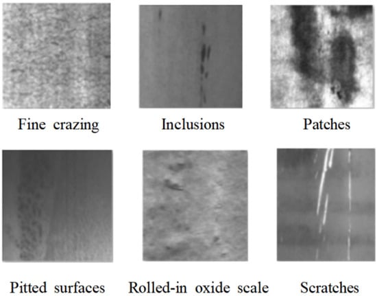
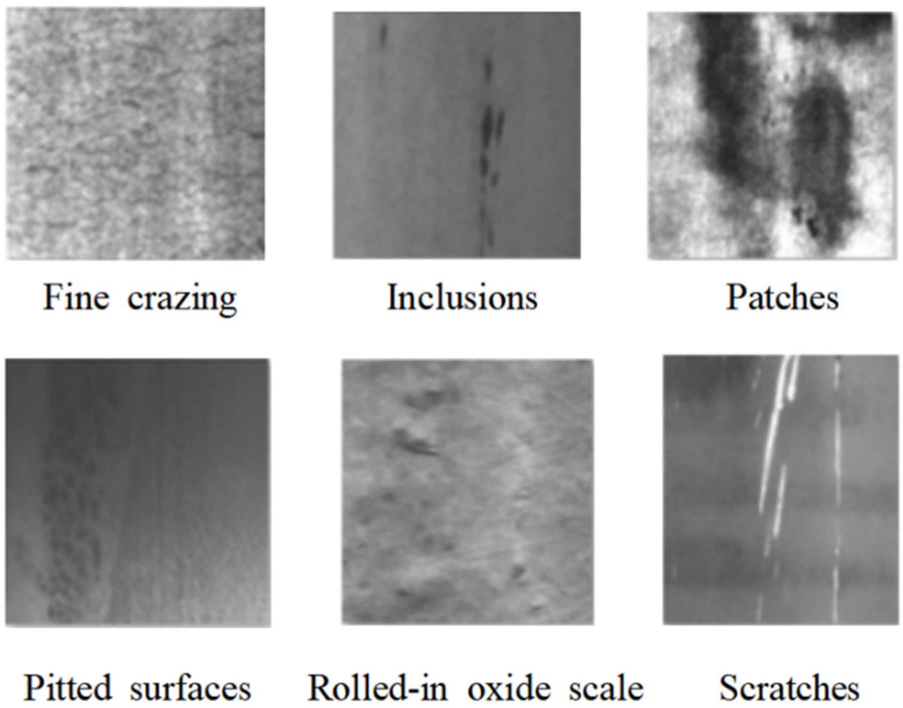
The relevant types of equipment surface damage considered in this study comprised fine crazing, inclusions, patches, pitting, rolled-in oxide scale, and scratches, each of which exhibits unique visual characteristics, as shown in Figure 1. Fine crazing appears as elongated linear structures, typically ranging from 0.1 to 0.5 mm wide, that exhibit poor contrast in grayscale images. Edge continuity inclusions are foreign objects embedded in the equipment surface exhibiting irregular block shapes with colors and textures that obviously differ from those of the substrate. Patches of brightness produce large areas of relatively uniform abnormal color with poor texture uniformity, obvious brightness changes, and blurred boundaries with the surrounding area. Pitted surfaces contain a considerable quantity of discrete corrosion pits appearing as densely distributed spots with multiple irregular edges. Rolled-in oxide scale is an irregular flaky structure attached to the surface that exhibits obvious texture directionality and typically presents a layered structure. Finally, scratches appear as linear grooves ranging from several millimeters to several centimeters in length that exhibit lower grayscale values than the surrounding area, relatively clear edges, and gentle gradients.
Figure 1.
Example images of steel surface damage types.
3. Construction of the Seven-Dimensional Feature Fusion Model
3.1. Model Definition
The application of multi-feature fusion to the detection of equipment surface damage remains in the exploratory stage at present [31]. Therefore, a seven-dimensional feature fusion model for surface damage characterization was established in this study considering the visual aspects of the six evaluated types of equipment surface damage. The proposed model integrates information describing seven key features to construct a comprehensive and complementary feature vector for each type of damage. This approach overcomes the limited ability of a single feature to reflect more than the local attributes of damage, provides standardized and highly distinguishable input for the subsequently applied classification algorithm, and improves detection efficiency in low-complexity scenarios. By considering the mean intensity, standard deviation (STD) of intensity, Fourier energy, edge density, local binary pattern (LBP) entropy, gradient magnitude, and fractal dimension features together, this model effectively addresses the insufficient characterization capability of traditional single-dimension feature models, difficulty of fully capturing complex damage features, poor detection algorithm input quality, and limited adaptability associated with other intelligent damage detection approaches. Because there is no unified numerical standard for the high and low values of the seven considered features, the distribution interval for each feature was determined as detailed in this section.
- (1)
- Mean intensity [32]
The mean intensity feature reflects the overall brightness of the damaged area, indicating the extent to which each type of damage is defined by the brightness of the reflective material (e.g., low intensity brightness indicates a depression). The mean greyscale intensity, which typically ranges from 0 to 255, is calculated as follows:
where () is the grayscale intensity value of the i-th pixel in the damage area and is the total number of pixels.
- (2)
- STD intensity [33]
The STD intensity feature quantifies the degree of dispersion and uniformity of the greyscale values inside a damage area. For example, patches with uneven color shades and complex pitting comprising alternating light and dark spots exhibit high STD intensity values, indicating strong contrast and inhomogeneity inside the area, whereas rolled-in oxide scale, single inclusions, and shallow and uniform scratches exhibit low STD intensity values, indicating high uniformity inside the area. The STD grayscale intensity is calculated as follows:
- (3)
- Fourier energy
The Fourier energy feature reflects the relative intensity of the high-frequency components in the image, such as details, edges, and textures, which correspond to regions with sharp grayscale variations, and is primarily used to evaluate texture periodicity and roughness. A high Fourier energy indicates that the image contains many textures, which is a typical feature of fine crazing and rolled-in oxide scale, whereas a low Fourier energy indicates that the image is smooth or the texture within lacks periodicity, which is common for inclusions, simple scratches, and certain patches. The Fourier energy is calculated as follows:
where is the logarithmic magnitude spectrum, which is used to enhance visualization and reduce the numerical dynamic range, and are frequency domain coordinates representing horizontal and vertical frequency components is the high-frequency region, defined as the area outside the central region, where the boundary of this central region serves as the cutoff value—frequencies inside are excluded (low-frequency) and frequencies outside are retained (high-frequency); and are the image height and width in pixels; and is the total energy. The final feature value represents the ratio of high-frequency energy to total energy.
- (4)
- Edge density [34]
The edge density feature quantifies the number of edge pixels per unit area and reflects the complexity and continuity of the damage contour. A high edge density is a strong indicator of fine crazing owing to the presence of dense network edges; a low edge density indicates sparse edges, such as those found in wide and shallow scratches, large-area uniform inclusions, or rolled-in oxide scale with periodic textures but poor edge contrast. The edge density is calculated as follows:
where F is the number of edge pixels detected by an edge detection operator, W and H are the width and height of the image, respectively, and D is the final calculated edge density (i.e., the ratio of edge pixels to total pixels).
- (5)
- LBP entropy [35]
The LBP entropy feature measures the randomness, complexity, and irregularity of the surface texture. A high LBP entropy indicates a complex, disordered, and random texture, such as that typical of patches and pitted surfaces; a moderate LBP entropy indicates a regular but complex texture, such as that for fine crazing; a low LBP entropy indicates a uniform, simple, and ordered texture, such as that observed in the directional texture of rolled-in oxide scale, uniform scratches, and single inclusions. The LBP entropy is calculated as follows:
where is the probability of the k-th LBP.
- (6)
- Gradient magnitude [36]
The gradient magnitude feature reflects the average intensity and sharpness of the edges in a damage area. A high gradient magnitude indicates a steep change in intensity, reflecting the sharp edges common in fine crazing, deep pitting, and high-contrast patches; a low gradient magnitude indicates a gentle change in intensity with fuzzy edges, which is common in shallow scratches, rolled-in oxide scale, and inclusions with a high degree of background fusion. The gradient magnitude is calculated as follows:
where is the morphological gradient value at the coordinates .
- (7)
- Fractal dimension [37,38]
The fractal dimension feature quantifies the geometric complexity and space-filling capacity of the surface structure and is notably scale-invariant. A high fractal dimension indicates an extremely rough, complex, and irregular surface, which is typical of fine crazing with a network structure and pitted surfaces with complex pits and patches; a low fractal dimension indicates a relatively smooth and simple surface, which is typical of rolled-in oxide scale (although scale has a texture, it typically exhibits high self-similarity), smooth scratches, and simple inclusions. Based on fractal theory, the selection of box-counting scales needs to cover the multi-level structure of image texture. This study adopts four scales of 2, 4, 8, and 16 pixels, forming a geometric progression with a common ratio of 2: the smallest scale of 2 pixels captures the fine irregularities of damage edges; the largest scale of 16 pixels reflects the macroscopic texture-filling characteristics; the intermediate scales ensure the continuity of multi-resolution analysis. This choice balances the resolution constraints of 200 × 200 pixel images and computational efficiency, avoiding sensitivity to noise from excessively small scales while preventing loss of texture details from excessively large scales. The fractal dimension is typically calculated using the box-counting method at four scales (2, 4, 8, and 16 pixels) as follows:
where s is the box-counting scale ( ∈ {2, 4, 8, 16} in the code), is the multi-scale box count, and b is the intercept of the linear fitted regression line for the log(s) vs. log(N(s)) curve.
3.2. Feature Values of Common Surface Damage Types
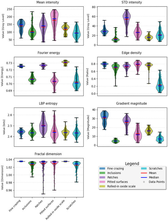
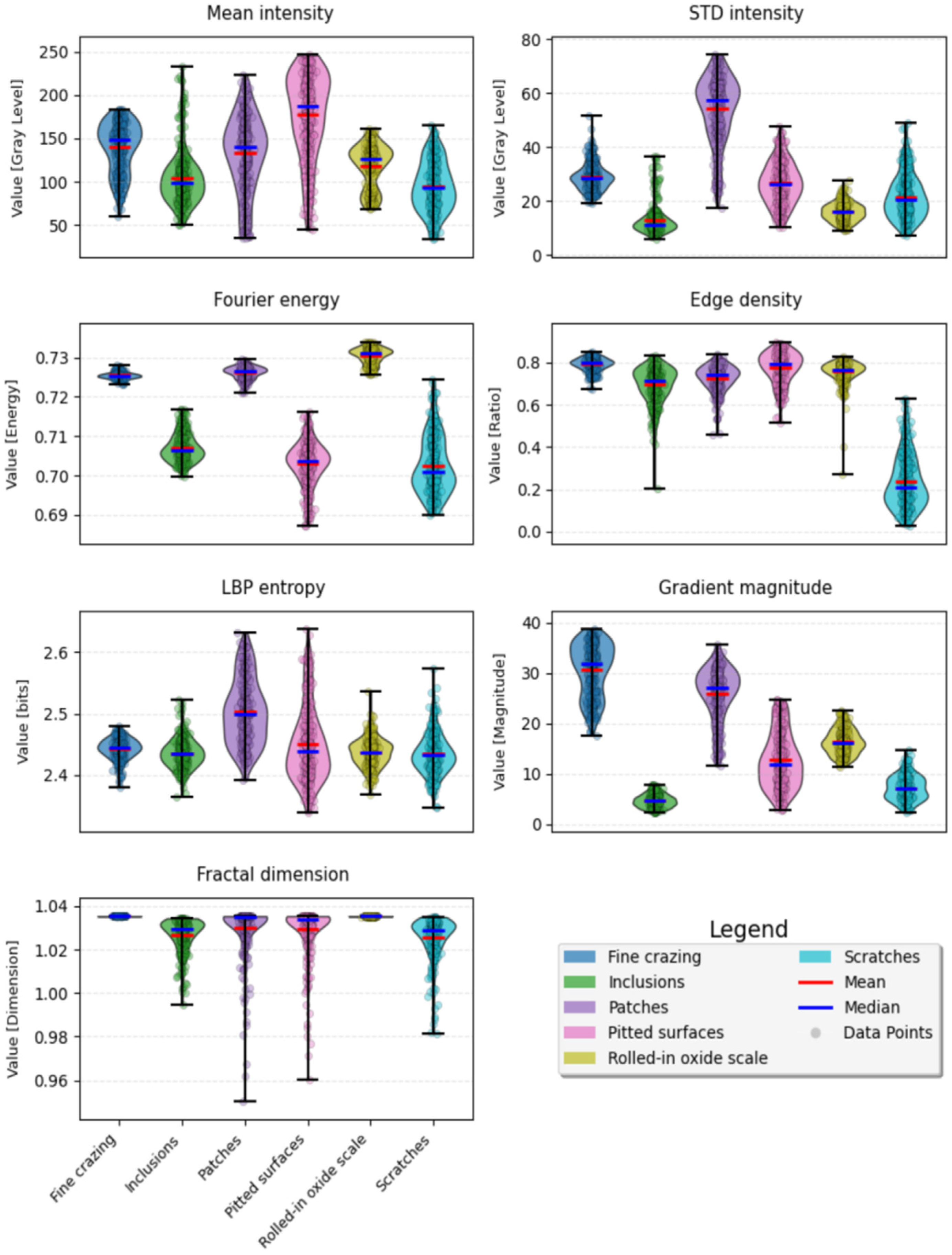
The effectiveness of the proposed method for intelligent surface damage detection was demonstrated by analyzing 1619 images of surface damage in a self-assembled dataset comprising 270 fine crack images, 268 inclusion images, 274 patch images, 276 pitted surface images, 265 rolled-in oxide scale images, and 266 scratch images. Based on these training samples, the seven feature values were extracted and statistically analyzed. The numerical ranges of the seven feature values for the damage types in the image set were determined and are listed in Table 1. Furthermore, a statistical analysis was performed on the extracted feature values to obtain the distribution histograms shown in Figure 2.
Table 1.
Characteristics of typical equipment surface damage types.
Figure 2.
Characteristic distributions of seven features for different types of surface damage.
The contents of Table 1 and Figure 2 indicate that although the seven features exhibited different values and distribution characteristics for each considered type of surface damage, the type of surface damage could not be readily identified using any single feature; therefore, damage type identification was carried out by fusing multiple features. Indeed, the results in Table 1 and Figure 2 suggest that the constructed seven-dimensional feature model can provide distinguishable feature vectors for different types of damage. Notably, these feature vectors can serve as standardized input for the subsequent classification algorithm and represent the key premise for achieving high-precision damage identification in this study accordingly.
4. Design and Implementation of the Recognition Algorithm
Different types of typical equipment surface damage were effectively identified in this study using a proposed image recognition algorithm based on seven-dimensional feature fusion. The overall process employed by the algorithm comprises three key stages: image preprocessing and feature extraction, feature management and normalization, and damage classification and confidence calculation using Bayesian averaging of kernel density estimation (KDE).
4.1. Image Preprocessing and Feature Extraction
First, the acquired color images are converted to grayscale by compressing the three-channel color information into single-channel intensity values. This step reduces computational complexity and directs attention to the texture and structural features relevant to the damage, rather than color information.
Next, the aforementioned seven feature quantities that effectively characterize the statistical properties, texture complexity, and structural irregularity of the images are extracted to form a comprehensive feature vector.
4.2. Feature Management and Normalization
The considerable differences among the scales and ranges of the extracted feature values can cause features with large ranges to dominate the classification process when they are directly used for classification. Therefore, all successfully extracted features are normalized before they are stored in the database. The min–max normalization method is applied to linearly transform the value of each feature into the interval [0, 1] as follows:
where X is the original feature value and and are the minimum and maximum values, respectively, of that feature for all samples in the database.
The normalized feature values are stored in the database together with the original feature values to provide standardized input for damage classification.
4.3. Damage Classification and Confidence Calculation
The damage classification and confidence calculated using the proposed Bayesian probabilistic model based on adaptive KDE [39] represent the core decision-making information provided by the proposed method for the intelligent detection of equipment surface damage. This model calculates the conditional probability densities of various types of damage based on the seven feature dimensions extracted and normalized in the previous stage, then applies Bayes’ theorem [40] to calculate the posterior probability determining the damage type in the evaluated image. The classified damage type is output along with the posterior probability of its determination to represent the confidence. The damage classification and confidence calculation process comprises the following five steps.
- (1)
- Obtain the training set via five-fold cross-validation.
Randomly divide the image data X for a single damage type into five non-overlapping subsets , each containing approximately the same number of samples. Take one subset at a time as the validation set and combine the remaining four subsets into the training set ; for example, if = , = . Repeat this process five times to obtain a full training set for cross-validation.
- (2)
- Calculate the KDE probability density for a single damage type [41].
Calculate the KDE probability density by constructing a smooth and continuous “density” function from a limited set of discrete data points through “stacking” using a standard function called the “kernel” to estimate the true but unknown overall probability distribution as follows:
where zi is the standardized vector of the i-th training sample (seven-dimensional, zi ∈ R7), h is the candidate bandwidth used to describe the feature distribution law of the damage. The bandwidth search range is set as [0.1, 2.0], which covers the full spectrum from under-smoothing (h → 0.1, where density estimation is sensitive to local fluctuations) to over-smoothing (h → 2.0, where density estimation approaches the global average). This range effectively captures the multi-scale distribution characteristics of the seven-dimensional normalized features (each dimension normalized to [0, 1]) in the feature space. The initial value is set to 0.1, starting from a relatively fine density structure, and the optimal bandwidth is automatically selected by traversing candidate bandwidths with a uniform step-size grid search, evaluated through five-fold cross-validation and the average log-likelihood criterion, d is the number of feature dimensions (i.e., 7), and is the kernel function value of the i-th training sample, which is calculated as follows:
where is the L2 norm (Euclidean distance) of the standardized vector and is calculated as .
Subsequent logarithmic calculation and division errors caused by excessively small density values can be prevented by setting the lower limit of the KDE probability density to 10−10, i.e.,
- (3)
- Calculate the average log-likelihood of the candidate bandwidths.
Traverse each sample in the corresponding validation subset Xval divided in step (1) to calculate the KDE probability density for each sample, then use the natural logarithm of the KDE probability density to obtain the single-fold log-likelihood, given by
Next, obtain the total log-likelihood by accumulating the single-fold log-likelihoods of the five cycles as follows:
Furthermore, eliminate the influence of the number of samples and obtain the average fitting effect of the bandwidth by calculating the average log-likelihood as follows:
where N is the total number of samples for a single damage type.
- (4)
- Select the optimal bandwidth.
Consider all candidate bandwidths within 0.1–2.0 to select the bandwidth with the maximum as the optimal bandwidth .
- (5)
- Calculate the posterior probability.
Finally, select the damage type with the maximum posterior probability to identify the type of damage in the image and use the value of the maximum posterior probability to represent the confidence. The posterior probability can be determined by
where is the joint probability of damage type , calculated as
in which is the optimal KDE probability density determined using the optimal bandwidth and is the prior probability calculated as the ratio of the number of damage type training samples to the total number of training samples , and is the evidence factor calculated as the sum of the joint probabilities for all valid damage types as follows:
where 10−20 is used as the lower limit to avoid division by zero errors caused by excessively small sums approaching 0.
5. Verification and Evaluation
5.1. Verification Results
The image dataset used in this study is a private dataset. All images are local views cropped to the damage region; background removal was uniformly completed during the data acquisition stage and is not part of the proposed method’s pipeline. The proposed method directly performs feature extraction and classification on images focused on the damaged area. The images have a uniform resolution of 200 × 200 pixels. All samples were acquired under the same standardized acquisition process, ensuring high consistency of imaging conditions across samples. The images were uniformly converted to grayscale format for subsequent analysis.
The assembled dataset contained 1799 images that were randomly divided into training and test sets at a ratio of approximately 9:1. As a result, the training set comprised 1619 images that were used to inform the statistical analysis of the seven-dimensional feature model, calculate the prior probabilities, and optimize the KDE bandwidth; the test set comprised 180 images that were used in the final performance evaluation and comparative experiments. Each image in the training set was labeled with the correct damage type to provide reliable feature statistics for classifier training. During training, the ranges for the seven features in each image were calculated, then stored in the database to reflect the ranges corresponding to the different types of damage, and the prior probability and optimal bandwidth for each type of damage were calculated.
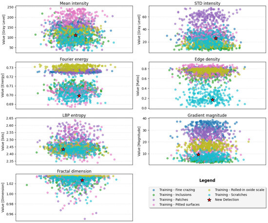
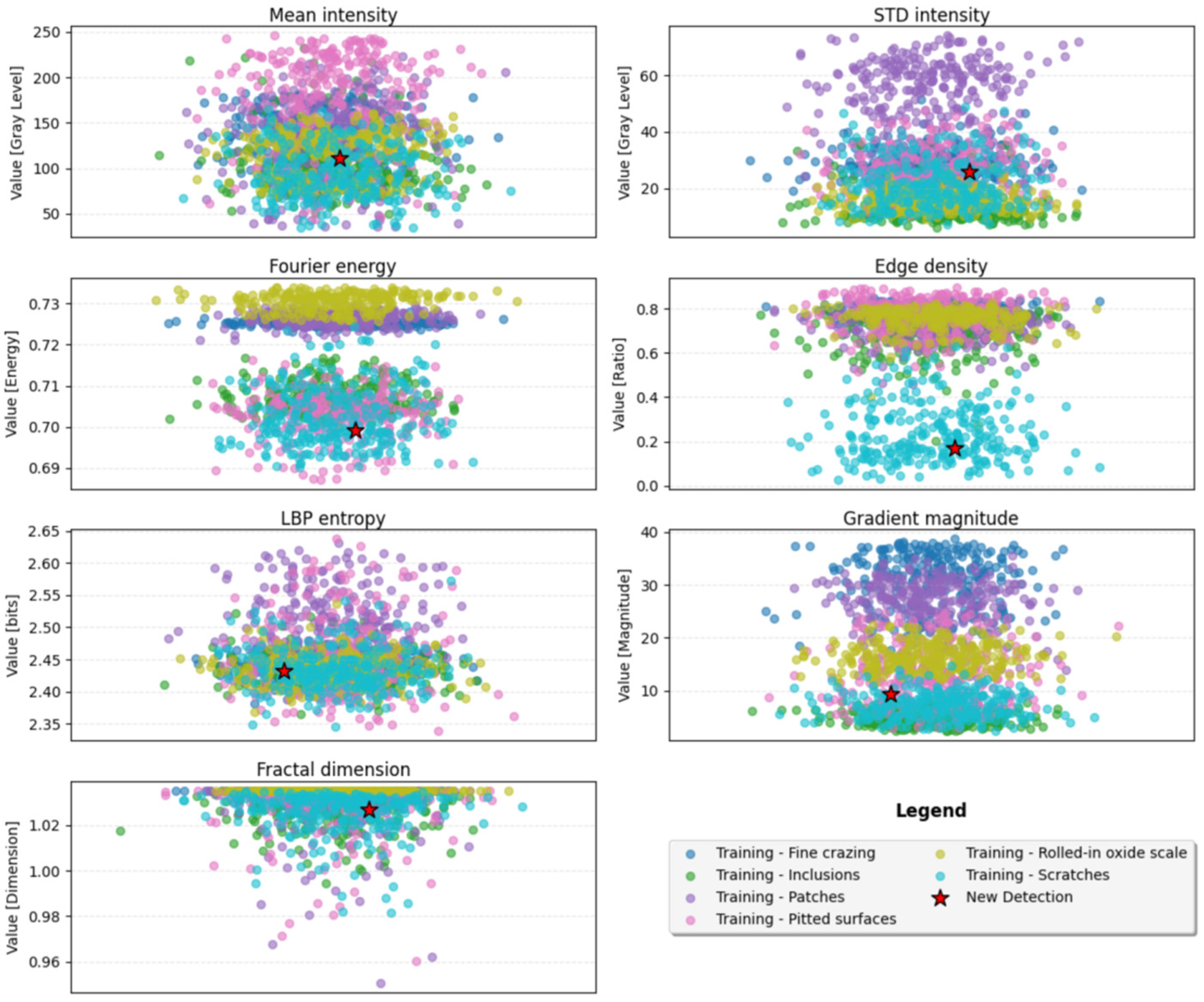
Taking a single defect image as an example, the seven feature dimensions of the image were first obtained and displayed relative to the ranges of the trained feature values, then the Bayesian probability was calculated to classify the damage type and calculate its confidence, as shown in Figure 3. Each diagram in this figure corresponds to one of the seven features defined in Section 3.1; the different colors represent the feature distributions for the six types of damage in the training set, and the red five-pointed stars represent the specific value sampled from the example image for each feature.
Figure 3.
Distribution of seven-dimensional feature values of a single damaged image across the training ranges of different damage types.
The results presented in Figure 3 indicate that all seven feature values for the example image fell well within the feature distributions for scratches in the training set. The edge density and gradient magnitude diagrams show sample points within the high-value area of the distribution, which is consistent with the actual damage characteristics of the example image. This result intuitively verifies three critical aspects of the proposed method: first, the seven-dimensional feature extraction process effectively captures the key visual attributes of damage; second, the extracted feature values follow reasonable distribution laws; third, the feature space of the example exhibited suitable consistency with that of the training set, providing a solid foundation for accurate classification using the probabilistic model.
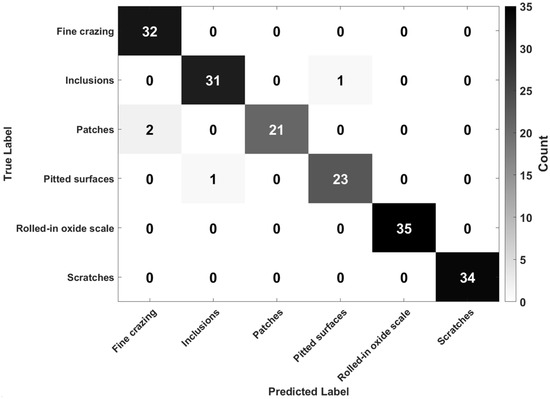
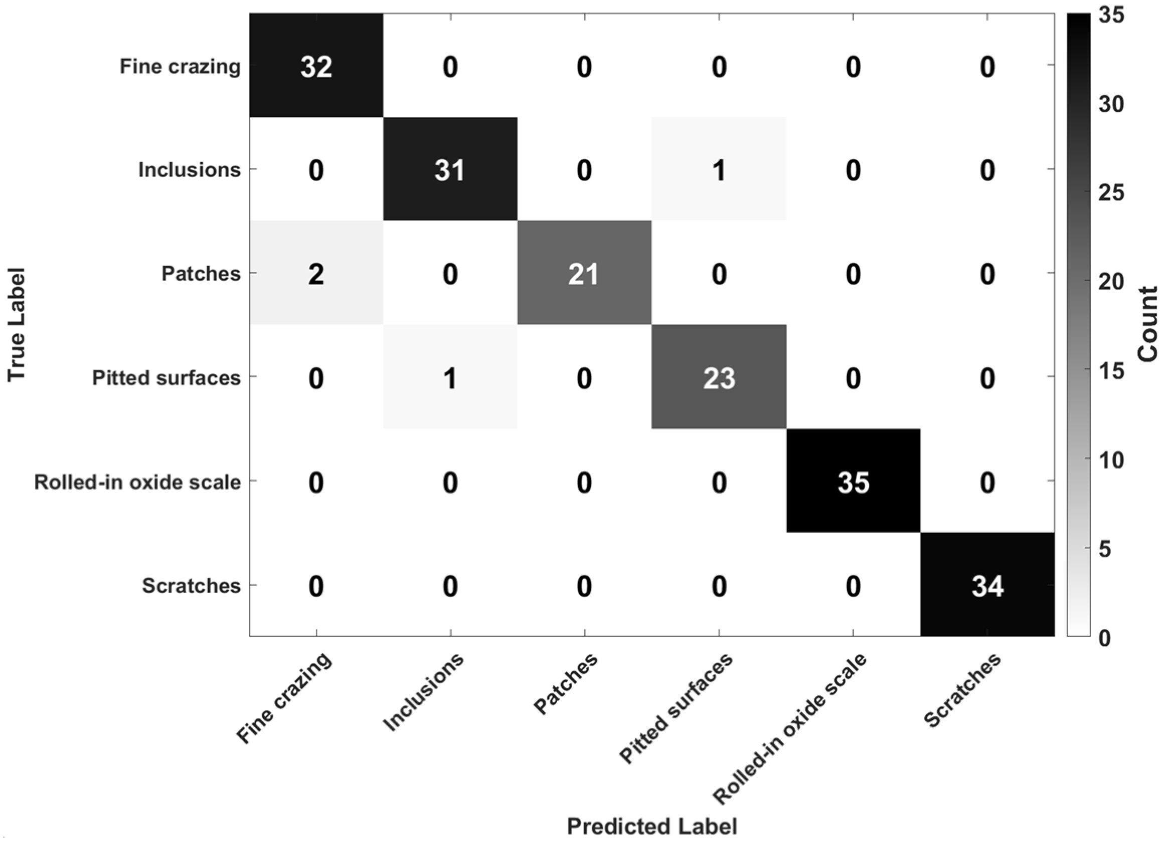
Applying the seven-dimensional feature extraction model to the 180 test set images indicated that the proposed damage detection algorithm exhibited suitable performance, with 176 samples correctly identified and only 4 samples misclassified for an overall accuracy of 97.77%. The specific results are shown in Figure 4: one inclusion defect was misjudged as a pitted surface defect, one pitted surface defect was misjudged as an inclusion defect, and two patch defects were misidentified as fine crack defects.
Figure 4.
Confusion matrix heatmap comparing typical surface damage/defect detection results.
Note that the dynamic updatability of the proposed detection model can be ensured by manually reviewing newly obtained images to add samples with correct identifications to the database, re-optimizing the bandwidth, and calculating the probability in the next detection; this improves classification accuracy and adaptability in practical applications.
It should be noted that in actual equipment maintenance workflows, damage identification typically follows a “classify first, then detect” sequence: the damage type is first determined, followed by quantitative detection and evaluation tailored to that specific type. Since the damage regions have already been extracted and cropped, the classification stage itself directly accomplishes the detection of surface damage faults; therefore, this study focuses on precisely this stage, realizing damage detection through feature extraction and type classification on pre-cropped images.
5.2. Evaluation
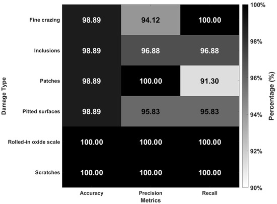
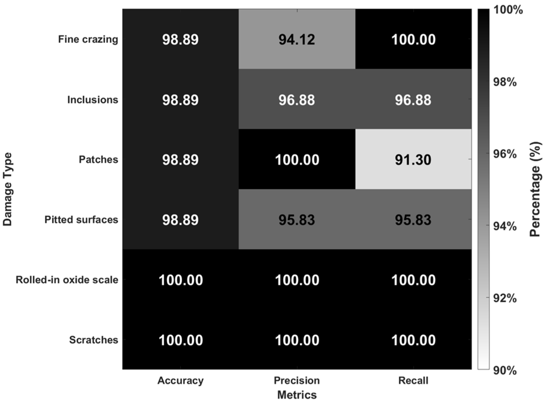
In terms of overall performance, the proposed method identified all damage types in the test set with a minimum accuracy of 98.89%, where this accuracy is calculated using the total number of such damages as the denominator. A heat map comparing the identification performance for each damage type in terms of accuracy, precision, and recall is shown in Figure 5. The identification of rolled-in oxide scale and scratch damage was perfect, with an accuracy, precision, and recall of 100%, indicating that the model produced no missed or false reports when identifying these two types of damage. However, the identification performances for other types of damage differed in various aspects. The recall for the identification of fine crazing was 100%, indicating that all samples exhibiting this type of damage were successfully identified with no missed reports, but the precision was relatively low at 94.12%, indicating that a small number of other damage types were misidentified as fine crazing. Conversely, the precision for the identification of patches was 100%, indicating that all images containing this type of damage were correctly identified by the model, but the recall of 91.30%—the lowest for the six types of damage—indicates that approximately 8.7% of actual patch damage instances were misclassified as other types. The identification performance for inclusions and pitted surfaces was relatively balanced, with the precision and recall values for both types of damage exceeding 95%, indicating that the model exhibited stable recognition ability for these types of damage while effectively controlling the occurrence of false and missed reports. These results confirm that the proposed damage detection model based on multi-feature fusion exhibits excellent performance in terms of accuracy, precision, and recall to provide efficient and stable recognition of multiple damage types, representing an effective and practical method for the industrial detection of most apparent surface damage. However, no more than 276 samples were provided in the training set for each type of damage, making the proposed model prone to overfitting and suggesting room for further optimization.
Figure 5.
Damage type identification performance in terms of accuracy, precision, and recall.
5.3. Comparative Experiments and Analysis
To ensure a fair comparison, all three methods (the proposed method, DNN, and AFA) were trained and tested using the same seven-dimensional feature database extracted from the image dataset. Two representative methods were selected for comparison: one is a deep learning method based on a deep neural network (DNN) [42], which serves as a typical representative of deep learning classifiers to verify the competitiveness of the proposed Bayesian probabilistic classification strategy against automatically learned decision boundaries in a fixed low-dimensional feature space; the other is the Ant Forest Algorithm (AFA), a meta-heuristic optimization classification method that borrows the idea of feature selection from ant colony systems [43]. By simulating ant foraging behavior and integrating random forest ensemble strategies for feature optimization and classification, AFA serves as a typical representative of swarm-intelligence-based optimization in traditional machine learning, allowing evaluation of the advantages of the proposed Bayesian probabilistic classification strategy. The selection of these two methods covers both mainstream technical routes of deep learning and traditional optimization, providing effective performance references under limited experimental conditions. More extensive comparisons, such as with other deep learning architectures (e.g., ResNet, Vision Transformer) or traditional classifiers (e.g., SVM, Random Forest), can be explored as future work.
The detailed configurations of the two comparative methods are as follows. The DNN is a 5-layer fully connected network with four hidden layers: input layer (7-dimensional) → 128 (ReLU + BatchNorm + Dropout 0.3) → 64 (ReLU + BatchNorm + Dropout 0.3) → 32 (ReLU + BatchNorm + Dropout 0.2) → 16 (ReLU + Dropout 0.2) → output layer (Sigmoid/Softmax). The optimizer is Adam with a learning rate of 0.001, the loss function is categorical cross-entropy, and an L2 regularization coefficient of 0.001 is used. Training employs early stopping (patience = 15) and learning rate decay (factor = 0.5, patience = 10), with a batch size of 32 and a maximum of 100 epochs. The AFA is an ensemble classifier comprising 30 ants and 50 decision trees with a maximum depth of 10. Each tree selects split features according to the feature probabilities derived from the ants, and the Gini index determines the split threshold. The process runs for 50 iterations, where five-fold cross-validation updates feature importance in each round. The ant probabilities are updated with a learning rate of 0.1 toward the importance values, and the final prediction is obtained by majority voting.
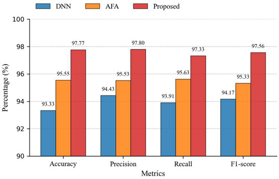
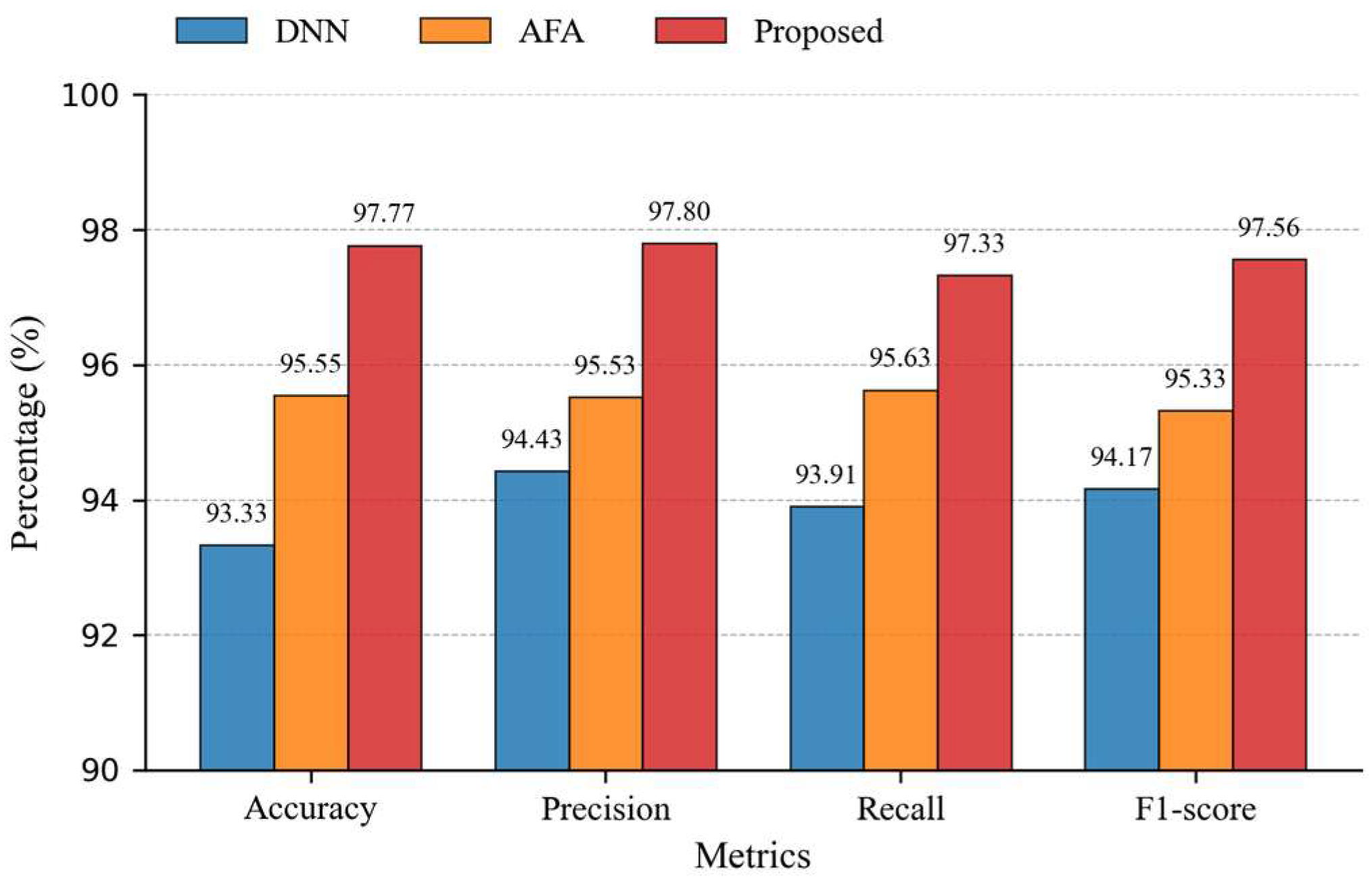
The results of this comparison are presented in Table 2 and Figure 6, where the comprehensive accuracy, precision, recall, and F1-score are calculated based on a total of 180 images in the test set as the denominator. The results show that the proposed method outperformed the DNN by 4.44%, 3.37%, 3.42%, and 3.39% in terms of comprehensive accuracy, precision, recall, and F1-score, respectively, and outperformed the AFA by 2.22%, 2.27%, 1.70%, and 2.23%, respectively, compared to those obtained by the AFA. These results indicate that the proposed seven-dimensional feature fusion and adaptive KDE-based Bayesian classification strategy developed and demonstrated in this study can more effectively utilize artificially designed discriminative features to achieve excellent classification performance based on a limited number of samples. This suggests that the proposed model represents significant progress in terms of overall classification accuracy, reduced false reports, and reduced missed reports.
Table 2.
Classification performance comparison results.
Figure 6.
Classification performance comparison results.
In terms of computational efficiency, the proposed method also exhibits advantages. Under the same testing environment, the per-sample feature extraction time of the proposed method is approximately 0.04 s, classification inference time approximately 0.04 s, resulting in a total processing time of about 0.08 s. It requires only 500 KB of storage to save the feature database and can run entirely on a standard CPU platform. In contrast, the DNN method requires about 0.12 s per sample for inference; the AFA method, due to the iterative optimization process, takes significantly longer per sample. Therefore, the proposed method demonstrates comprehensive efficiency advantages in inference speed, storage overhead, and hardware requirements for practical deployment.
To further verify the influence of different training/test set split ratios on model performance, we conducted an additional experiment with an 8:2 split (training set 1439 images, test set 360 images). The results indicate that under this split ratio, the model achieved a comprehensive accuracy of 97.77%, precision of 97.98%, recall of 97.70%, and F1-score of 97.79%, which are essentially consistent with the 97.77% obtained under the 9:1 ratio. The precision and recall for each damage category also showed no significant fluctuations.
Regarding overfitting control and generalization capability, several points need to be clarified. First, at the methodological design level, the adoption of a seven-dimensional handcrafted feature fusion strategy results in a model parameter scale much smaller than deep learning networks, fundamentally reducing the risk of overfitting. Additionally, the kernel density estimation bandwidth optimization process incorporates five-fold cross-validation and the average log-likelihood criterion, effectively preventing over-adaptation of density estimation to training data. Second, at the experimental verification level, as mentioned above, the model accuracy remained highly consistent at 97.77% under both 9:1 and 8:2 split ratios, demonstrating insensitivity to data partitioning. Moreover, although the training and test sets in this study were collected from the same standardized imaging setup to ensure reliability of feature extraction, the test results are entirely based on generalization inference on unseen samples, without any “rote memorization” tendency. In summary, the proposed method exhibits good generalization stability under limited sample conditions.
It should be noted that this study focuses on the classification of already-cropped damage regions, which is fundamentally different in task definition from pixel-level semantic segmentation-based damage detection methods (e.g., U-Net [44]). The former takes a damage region image as input and outputs a single class label; the latter takes an entire raw scene image as input and predicts damage location and class pixel by pixel. There are significant differences in input form, output granularity, and evaluation metrics between the two, making direct performance comparison inappropriate. Combining the proposed feature fusion model with lightweight segmentation networks to extend from region classification to pixel-level localization is a promising direction worth exploring.
6. Conclusions
This study proposed an intelligent equipment surface damage detection method based on multi-feature fusion and a Bayesian probabilistic model employing adaptive KDE. The primary contributions and conclusions of this study are as follows:
- (1)
- A seven-dimensional feature model was constructed to systematically characterize six typical types of damage considering the mean intensity, STD of intensity, Fourier energy, edge density, LBP entropy, gradient magnitude, and fractal dimension features. The use of multiple feature dimensions was intended to overcome the insufficient ability of other identification models to characterize damage using single features.
- (2)
- An adaptive KDE-based Bayesian classifier was proposed to accurately identify damage type and provide a quantitative measure of confidence using bandwidth optimization and a Bayesian decision-making mechanism.
- (3)
- Experiments conducted using a self-assembled dataset showed that the comprehensive identification accuracy provided by the proposed method reached 97.77%, which was superior to that of either the DNN or AFA damage identification methods when considering multiple indicators, verifying its superior effectiveness.
The results of this study are expected to inform the development of improved methods for detecting surface damage on wear- and degradation-prone steel components, such as those used in military applications. Notably, the ability to accurately identify multiple types of surface damage using seven feature dimensions represents a critical capability lacking in previous approaches for damage detection.
However, note that this study employed an idealized dataset comprising images with simple backgrounds and stable illumination, and the generalization ability of the proposed method when provided with images containing complex backgrounds, variable illumination, and highly reflective surfaces remains to be verified. Furthermore, due to the constraints of the dataset acquisition conditions, this study did not establish an accurate calibration relationship between image pixels and physical scale, which to some extent limits the quantitative evaluation of damage geometric features. The ability of the proposed method to detect early microscopic damage exhibiting weak features (such as microcracks narrower than 0.1 mm) must be explored. Therefore, future work will focus on expanding the diversity of the model training dataset, establishing pixel-to-millimeter mapping through imaging system calibration, exploring the use of an adaptive feature selection mechanism, and attempting to incorporate lightweight deep learning models into the proposed method.
Author Contributions
Conceptualization, L.C. and F.Z.; methodology, L.C. and X.H.; software, F.W. and X.H.; validation, F.Z. and F.W.; formal analysis, F.W.; investigation, F.Z.; resources, X.L.; data curation, S.H.; writing—original draft preparation, X.H.; writing—review and editing, L.C. and F.W.; visualization, F.W. and X.H.; supervision, L.C.; project administration, L.C.; funding acquisition, L.C. All authors have read and agreed to the published version of the manuscript.
Funding
This work was supported by The National Key Laboratory of Unmanned Aerial Vehicle Technology, Grant-No. WRJK202506.
Data Availability Statement
The original contributions presented in this study are included in the article. Further inquiries can be directed to the corresponding author.
Conflicts of Interest
The authors declare no conflict of interest.
References
- Doig, A. Military Metallurgy; Department of Materials and Medical Sciences, Cranfield University: Cranfield, UK, 2020. [Google Scholar]
- Ma, X.Y.; Li, R.; Li, Z.L.; Zhai, W.Z. LF-YOLO for strip surface defect detection in industrial scenarios. Comput. Eng. Appl. 2024, 60, 78–87. [Google Scholar] [CrossRef]
- Yang, S.; Xie, Y.; Wu, J.; Huang, W.; Yan, H.; Wang, J.; Bi, W.; Yu, X.; Wu, Q.; Xie, F. CFE-YOLOv8s: Improved YOLOv8s for Steel Surface Defect Detection. Electronics 2024, 13, 2771. [Google Scholar] [CrossRef] [Scilit]
- Guo, Z.; Wang, C.; Yang, G.; Huang, Z.; Li, G.; Li, G. MSFT-YOLO: Improved YOLOv5 Based on Transformer for Detecting Defects of Steel Surface. Sensors 2022, 22, 3467. [Google Scholar] [CrossRef] [Scilit] [PubMed]
- Zhang, D.; Hao, X.; Wang, D.; Qin, C.; Zhao, B.; Liang, L.; Liu, W. An efficient lightweight convolutional neural network for industrial surface defect detection. Artif. Intell. Rev. 2023, 56, 10651–10677. [Google Scholar] [CrossRef] [Scilit]
- Hu, X.; Lin, S. DFFNet: A lightweight approach for efficient feature-optimized fusion in steel strip surface defect detection. Complex Intell. Syst. 2024, 10, 1623–1634. [Google Scholar] [CrossRef] [Scilit]
- Cui, Y.; Zhao, L.; Li, H.; Liu, H. Strip surface defect detection based on wavelet denoising and improved Canny algorithm. Mod. Electron. Tech. 2024, 47, 148–152. [Google Scholar] [CrossRef]
- Xu, H.B.; Feng, K.R.; Huang, L.; Xiong, L. Improved Otsu algorithm for rolling contact fatigue defect detection. J. Comput.-Aided Des. Comput. Graph. 2019, 31, 1130–1138. [Google Scholar] [CrossRef] [Scilit]
- Chen, Y.; Deng, C.; Chen, X. An Improved Canny Edge Detection Algorithm. Int. J. High Technol. 2025, 8. Available online: https://gvpress.com/journals/IJHIT/vol8_no10/33.pdf (accessed on 24 June 2026).
- Ustabaş Kaya, G.; Saraç, Z. Crack Detection by Optical Voice Recorder Based on Digital Holography. Photonic Sens. 2019, 9, 327–336. [Google Scholar] [CrossRef] [Scilit]
- Sun, Y.Y.; Yang, B.W.; Sima, K.; Mu, W.M.; Lei, L. Research on few-shot small target detection based on Faster R-CNN. Mod. Inf. Technol. 2025, 9, 67–71+77. [Google Scholar] [CrossRef]
- Xue, D.L.; Li, L.; Zhou, Z.J.; Chang, Y.S.; Xiang, Y.; Chen, D.Y. Steel surface defect detection and segmentation based on improved Mask R-CNN. Comput. Meas. Control 2025, 33, 47–53+75. [Google Scholar] [CrossRef]
- Sheiati, S.; Chen, X. Advances in computer vision-based structural health monitoring techniques for wind turbine blades. Renew. Sustain. Energy Rev. 2025, 224, 116078. [Google Scholar] [CrossRef] [Scilit]
- Luo, Q.; Fang, X.; Liu, L.; Yang, C.; Sun, Y. Automated visual defect detection for flat steel surface: A survey. IEEE Trans. Instrum. Meas. 2020, 69, 626–644. [Google Scholar] [CrossRef] [Scilit]
- Fu, J.; Zhu, X.; Li, Y. Recognition of surface defects on steel sheet using transfer learning. arXiv 2019, arXiv:1909.03258. [Google Scholar]
- Chen, Y.; Ding, Y.; Zhao, F.; Zhang, E.; Wu, Z.; Shao, L. Surface Defect Detection Methods for Industrial Products: A Review. Appl. Sci. 2021, 11, 7657. [Google Scholar] [CrossRef] [Scilit]
- Kaya, G.U. Development of hybrid optical sensor based on deep learning for detection and classification of micro-defects on printed circuit boards. Measurement 2023, 206, 112247. [Google Scholar] [CrossRef] [Scilit]
- Chen, X.; Sheiati, S.; Shihavuddin, A. AQUADA PLUS: Automated damage inspection of cyclic-loaded large-scale composite structures using thermal imagery and computervision. Compos. Struct. 2023, 318, 117085. [Google Scholar] [CrossRef] [Scilit]
- Sheiati, S.; Chen, X. Deep learning-based fatigue damage segmentation of wind turbine blades under complex dynamic thermal backgrounds. Struct. Health Monit. 2024, 23, 539–554. [Google Scholar] [CrossRef] [Scilit]
- Zhong, K.; Teng, S.; Liu, G.; Chen, G.; Cui, F. Structural Damage Features Extracted by Convolutional Neural Networks from Mode Shapes. Appl. Sci. 2020, 10, 4247. [Google Scholar] [CrossRef] [Scilit]
- Niu, S.; Zhou, X.; Zhou, D.; Yang, Z.; Liang, H.; Su, H. Fault Detection in Power Distribution Networks Based on Comprehensive-YOLOv5. Sensors 2023, 23, 6410. [Google Scholar] [CrossRef] [Scilit] [PubMed]
- Wang, H.J.; Tong, X. Med-SAMNet: A multi-scale feature fusion network for medical image segmentation. J. Yibin Univ. 2025, 25, 31–38. Available online: https://link.cnki.net/urlid/51.1630.Z.20250903.1225.002 (accessed on 24 June 2026).
- Wang, R.; Tang, Z.J. Wind turbine blade defect detection method based on multi-feature fusion and ensemble learning. Comput. Sci. 2025, 52, 470–477. [Google Scholar]
- Liu, A.; Wang, Z.Y.; Zhang, C.J.; Chu, J.L. Rainy railway vehicle image restoration method based on multi-scale feature fusion. Tech. Autom. Appl. 2025, 1–8. Available online: https://link.cnki.net/urlid/23.1474.TP.20250902.1407.030 (accessed on 24 June 2026).
- Cui, X.F.; Han, P.L.; Chang, Y.; Chen, K.J. Lightweight SAR image ship detection method based on multi-scale feature enhancement. Aerosp. Shanghai (Chin. Engl.) 2026, 43, 160–169. Available online: https://link.cnki.net/urlid/31.2169.V.20250826.1606.004 (accessed on 24 June 2026).
- Hu, Y.; Chen, Q.; Tao, T.; Li, H.; Zuo, C. Absolute three-dimensional micro surface profile measurement based on a Greenough-type stereomicroscope. Meas. Sci. Technol. 2017, 28, 045004. [Google Scholar] [CrossRef] [Scilit]
- Zhao, J.; Yu, J.; Chen, Y.; Da, F. Texture-immune 3D profilometry via FFT-guided morphological component analysis in single-shot fringe projection. Measurement 2026, 257, 118685. [Google Scholar] [CrossRef] [Scilit]
- Boikov, A.; Payor, V.; Savelev, R.; Kolesnikov, A. Synthetic Data Generation for Steel Defect Detection and Classification Using Deep Learning. Symmetry 2021, 13, 1176. [Google Scholar] [CrossRef] [Scilit]
- Luleci, F.; Catbas, F.N.; Avci, O. CycleGAN for Undamaged-to-Damaged Domain Translation for Structural Health Monitoring and Damage Detection. Mech. Syst. Signal Process. 2023, 197, 110370. [Google Scholar] [CrossRef] [Scilit]
- Ta, Q.-B.; Huynh, T.-C.; Pham, Q.-Q.; Kim, J.-T. Corroded Bolt Identification Using Mask Region-Based Deep Learning Trained on Synthesized Data. Sensors 2022, 22, 3340. [Google Scholar] [CrossRef] [Scilit] [PubMed]
- Liu, Q.; Zhang, X.F.; Jiang, H. HBGF-YOLO based infrared small target defect detection for UAV aerial photography of photovoltaic panels. Laser Optoelectron. Prog. 2026, 63, 170–184. Available online: https://link.cnki.net/urlid/31.1690.TN.20250714.1547.074 (accessed on 24 June 2026).
- Taniguchi, K.; Uet, A.; Tatsumi, S. A mura detection method. Pattern Recognit. 2006, 39, 1044–1052. [Google Scholar] [CrossRef] [Scilit]
- Prasanna, P.; Dana, K.J.; Gueunski, N.; Basily, B.B.; La, H.M.; Lim, R.S.; Parvardeh, H. Automated Crack Detection on Concrete Bridges. IEEE Trans. Autom. Sci. Eng. 2016, 13, 1240–1249. [Google Scholar] [CrossRef] [Scilit]
- Gao, J.; Liu, T.; Wang, X.F.; Du, H.W.; Shi, Z. TWRD-Net: A real-time detection network algorithm for traction wire rope defects. Chin. J. Sci. Instrum. 2023, 44, 223–235. [Google Scholar] [CrossRef]
- Liu, H.; Jia, X.; Su, C.; Yang, H.; Li, C. Tire appearance defect detection method via combining HOG and LBP features. Front. Phys. 2023, 11, 1099261. [Google Scholar]
- Malarvel, M.; Sethumadhavan, G.; Bhagi, P.C.R.; Kar, S.; Saravanan, T.; Krishnan, A. Anisotropic diffusion based denoising on X-radiography images to detect weld defects. Digit. Signal Process. 2017, 68, 112–126. [Google Scholar] [CrossRef] [Scilit]
- Wang, H.; Bu, Y.; Zhang, H.; Yang, X. Magnetic trace image defect detection based on fractal dimension. Appl. Res. Comput. 2015, 32, 603–605+612. [Google Scholar]
- Tang, B.; Chen, L.; Sun, W.; Lin, Z.-K. Review of surface defect detection of steel products based on machine vision. IET Image Process. 2023, 17, 303–322. [Google Scholar] [CrossRef] [Scilit]
- Cai, Z.Y.; Lu, B.L.; Xiong, S.Q.; Wang, W.Y. Lithology identification based Oil Bayesian probability using adaptive kernel density. Geophys. Geochem. Explor. 2020, 44, 919–927. [Google Scholar]
- Chung, H.; Lee, K. Detecting defects in composite beams and plates using Bayesian inference. Mech. Syst. Signal Process. 2014, 53, 50–62. [Google Scholar] [CrossRef] [Scilit]
- Lang, C.I.; Sun, F.K.; Lawler, B.; Dillon, J.; Al Dujaili, A.; Ruth, J.; Cardillo, P.; Alfred, P.; Bowers, A.; Mckiernan, A.; et al. One Class Process Anomaly Detection Using Kernel Density Estimation Methods. IEEE Trans. Semicond. Manuf. 2022, 35, 457–469. [Google Scholar] [CrossRef] [Scilit]
- Shin, S.; Jin, C.; Yu, J.; Rhee, S. Real-Time Detection of Weld Defects for Automated Welding Process Base on Deep Neural Network. Metals 2020, 10, 389. [Google Scholar] [CrossRef] [Scilit]
- Abd-Alsabour, N.; Randall, M. Feature selection for classification using an ant colony system. In Proceedings of the 6th IEEE International Conference on E–Science Workshops; IEEE Press: New York, NY, USA, 2010; pp. 86–91. [Google Scholar]
- Sheiati, S.; Nguyen, H.; Kinnunen, P.; Ranjbar, N. Cementitious phase quantification using deep learning. Cem. Concr. Res. 2023, 172, 107231. [Google Scholar] [CrossRef] [Scilit]

Disclaimer/Publisher’s Note: The statements, opinions and data contained in all publications are solely those of the individual author(s) and contributor(s) and not of MDPI and/or the editor(s). MDPI and/or the editor(s) disclaim responsibility for any injury to people or property resulting from any ideas, methods, instructions or products referred to in the content. |
© 2026 by the authors. Licensee MDPI, Basel, Switzerland. This article is an open access article distributed under the terms and conditions of the Creative Commons Attribution (CC BY) license.