Roller Trajectory Extraction and Error Compensation Based on Projection Method and Gaussian Process Regression

Abstract

To address the difficulty of directly applying finite element simulation trajectories to actual spinning machines, as well as the discrepancy between simulation data and equipment execution in the spinning process, this paper proposes a trajectory mapping method based on simulation trajectory extraction and data-driven error compensation. First, based on secondary development in ABAQUS, a discrete shell is introduced and combined with coordinate transformation to achieve accurate extraction of the roller center trajectory, and the simulated trajectory is converted into a discrete coordinate sequence. Subsequently, a roller trajectory acquisition and visualization system is developed, and machine motion data are collected and visualized for comparative analysis via the Modbus-RTU protocol. On this basis, to address the systematic deviation between simulated and actual execution trajectories, a trajectory error compensation method based on the projection method and Gaussian Process Regression is proposed. By modeling normal-direction errors and applying normal-direction compensation, smooth and stable optimization of the original simulation trajectory is achieved. Finally, experimental validation is conducted on a single-roller spinning machine, and the variation in trajectory deviation before and after compensation is comparatively analyzed. The results show that the proposed method effectively reduces trajectory execution errors, decreasing the average error from 0.503 mm to 0.229 mm, and significantly improves trajectory matching accuracy. This study provides an effective technical pathway for high-precision transformation of simulation trajectories to actual equipment in spinning processes and offers important support for the transition from experience-driven to model-driven spinning manufacturing.

1. Introduction

Spinning technology, as a typical continuous plastic forming process, possesses advantages such as high material utilization, low forming load, and suitability for near-net-shape forming of complex thin-walled axisymmetric components. It has been widely applied in aerospace, automotive manufacturing, energy equipment, and high-end precision manufacturing fields [1,2]. With the increasing demand for complex curved-profile components and lightweight thin-walled structures, the influence of roller trajectories on material flow, wall-thickness distribution, and surface quality has become increasingly significant, making trajectory design one of the key factors affecting forming accuracy and process stability [3,4,5,6]. Therefore, the rational design and precise control of roller trajectories have become important research topics in spinning technology.

At present, extensive studies have been conducted on roller trajectory design and forming behavior in conventional spinning processes, including pass planning, trajectory curve forms, and forming quality control. Hayama et al. [7] investigated pass planning in conventional spinning and pointed out that reasonable trajectory allocation contributes to improved forming stability. Ma et al. [8] analyzed the influence of different trajectory curves on forming quality and demonstrated that trajectory forms directly affect material flow and forming accuracy. Liu [9] further studied the relationship between roller trajectories and deformation mechanisms in multi-pass spinning processes, indicating that trajectory design plays an important role in forming stability.

With the development of spinning theory and numerical analysis methods, parameterized approaches have gradually been adopted for roller trajectory description and optimization. Xia et al. [10] employed involute trajectories to improve trajectory continuity and mandrel conformity during conical spinning. Liu et al. [11] proposed a geometrical method for roller trajectory construction, while Chen et al. [12] further applied multi-pass involute trajectory design to finite element simulation analysis. In addition, Liu et al. [13] introduced B-spline curves into spinning trajectory representation, enabling continuous fitting of complex trajectories and improving trajectory smoothness and machining stability. These studies indicate that appropriate trajectory functions are essential for improving material flow and forming stability.

Regarding trajectory influence and finite element simulation studies, Liu et al. [14] investigated the effects of different roller trajectories on stress–strain distribution and material flow behavior during conventional spinning. Wang et al. [15] further analyzed the influence of trajectory curves on spinning force and wall-thickness uniformity. Wei et al. [16] and Zhan et al. [17] studied the effects of roller loading trajectories on multi-pass spinning processes and wall-thickness variation, respectively. These studies demonstrate that roller trajectories are critical factors affecting forming quality and process stability.

In terms of roller trajectory design and forming optimization, Wang et al. [18,19] proposed trajectory correction methods based on trajectory compensation and interpolation optimization to improve trajectory continuity and machining stability.

With the development of intelligent manufacturing and data-driven methods, research on spinning trajectory optimization and trajectory error compensation has gradually evolved from traditional empirical design toward intelligent modeling and online optimization. Gondo et al. [20] proposed a roller path solving method based on multi-objective task-priority control, enabling the automatic generation and coordinated optimization of multi-pass spinning trajectories. Gao et al. [21] further developed an online intelligent roller path design method that achieved dynamic trajectory optimization and real-time adjustment through adaptive learning. In addition to trajectory design, trajectory error compensation has also attracted considerable attention in CNC machining. Liu et al. [22] proposed a contour error pre-compensation method based on global toolpath modulation to reduce trajectory tracking errors in multi-axis machining, while He et al. [23] further combined hybrid models for trajectory error prediction and compensation, thereby improving the execution accuracy of complex machining trajectories. Meanwhile, data-driven error modeling methods have gradually been introduced into machine tool error compensation. Wei et al. [24] established a thermal error compensation model for CNC machine tools based on Gaussian Process Regression (GPR), achieving high prediction accuracy and robustness. Wan et al. [25] further applied GPR to volumetric error compensation of machine tools, improving the modeling accuracy of complex error fields. Schwenke et al. [26] and Geng et al. [27] reviewed geometric error measurement and compensation techniques for machine tools, respectively, and pointed out that error compensation methods based on data-driven approaches and geometric feature constraints have become an important research direction in high-precision manufacturing. However, most existing studies focus on CNC machining or machine tool error compensation, while related research in spinning processes remains relatively limited. Existing methods mainly model coordinate-component errors or thermal errors of machine tools, with limited consideration of the local geometric characteristics of continuous spinning trajectories and trajectory error modeling based on local normal directions.

Compared with studies on roller path design, research on the consistency between finite element simulation trajectories and actual machine execution trajectories remains relatively limited. In practical spinning processes, CNC interpolation, coordinate mapping, and machine motion errors may lead to systematic deviations between the executed trajectory and the simulated trajectory, thereby affecting forming accuracy and process stability. Therefore, it is necessary to establish a mapping relationship between simulation trajectories and actual execution trajectories and to investigate trajectory error compensation methods.

Existing compensation approaches are primarily based on coordinate-component error modeling. However, for continuous curved trajectories in spinning processes, trajectory deviations are more likely to manifest as geometric deviations along the local normal direction of the trajectory rather than simple coordinate-component errors. Traditional methods have difficulty accurately characterizing such local geometric features, thereby limiting compensation accuracy.

To address the above issues, this study proposes a spinning trajectory mapping and compensation method based on simulated trajectory extraction and data-driven error modeling. First, ABAQUS secondary development is employed to extract the roller center trajectory and establish the mapping relationship between the simulated trajectory and the machine coordinate system. Subsequently, the projection method is adopted to extract the normal-direction error between measured trajectories and simulated trajectories, and a Gaussian Process Regression (GPR) model is introduced for error modeling and trajectory compensation. The primary focus of this work is not conventional forming-quality optimization, but rather the consistency problem between finite element simulated trajectories and actual machine execution trajectories, aiming to investigate the executability of simulated trajectories and corresponding trajectory compensation methods in practical spinning machines.

2. Trajectory Path Extraction Based on Finite Element Simulation

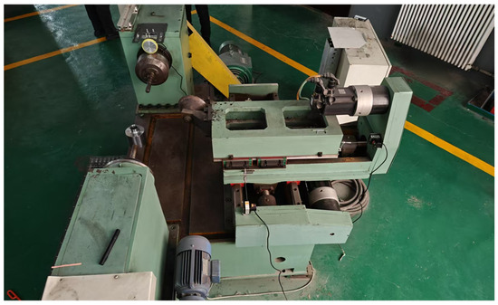
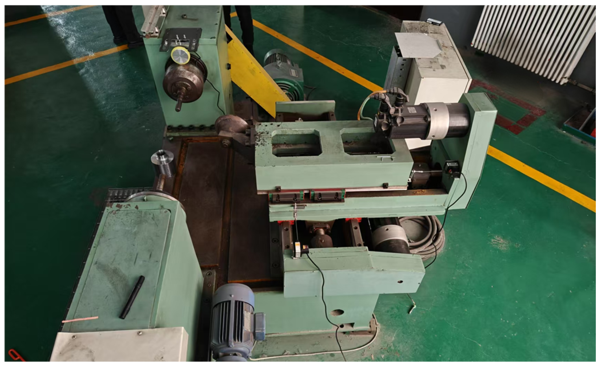
To obtain a roller motion trajectory that can be directly applied to actual machine tool execution, it is first necessary to establish a finite element model that accurately reflects the real spinning process and to perform forming simulations of the double-conical spinning part under appropriate process parameters. In this study, ABAQUS 2022 is employed as the simulation platform to conduct numerical simulation of the single-roller spinning process for the double-conical workpiece. The corresponding physical equipment is a single-roller spinning machine, as shown in Figure 1.The experimental system was a self-developed device from Changchun University of Science and Technology (Changchun, China). The subsequent trajectory extraction and mapping are primarily focused on the center motion trajectory of the roller during the forming process.

Figure 1. Single-Roller Spinning Machine.

2.1. Finite Element Simulation of Double-Conical Spinning Parts

Establishment of the Simulation Geometric Model and Determination of Process Parameters

• Establishment of Simulation Model

• Establishment of the Core Mold Simulation Model

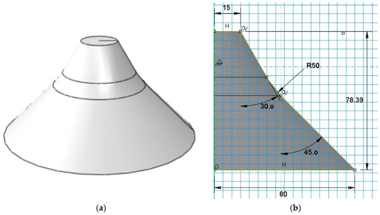
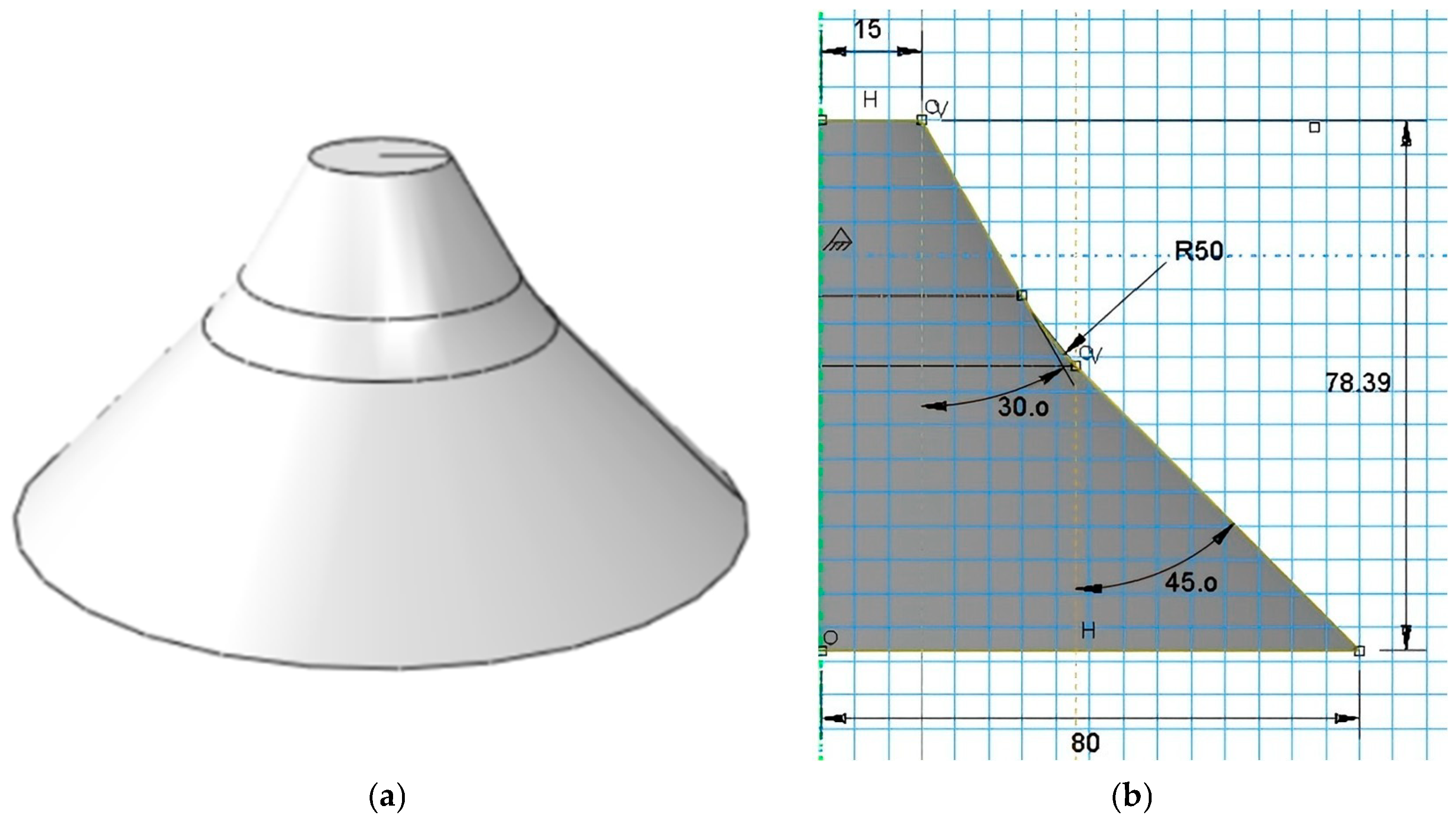
The geometric model of the core mold used in the spinning simulation of the double-conical cylindrical part is shown in Figure 2. The dimensional parameters of the profile are as follows: small-end diameter d = 30 mm, large-end diameter D = 160 mm, first half-cone angle = 30°, second half-cone angle = 45°, height H = 78.39 mm, and the transition arc radius between the conical sections r = 50 mm.

Figure 2. Core Mold Simulation Model. (a) Geometric Model of the Core Mold for Simulation. (b) Dimensional Parameters of the Core Mold Simulation.

• Establishment of the Blank Simulation Model

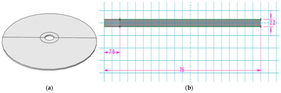
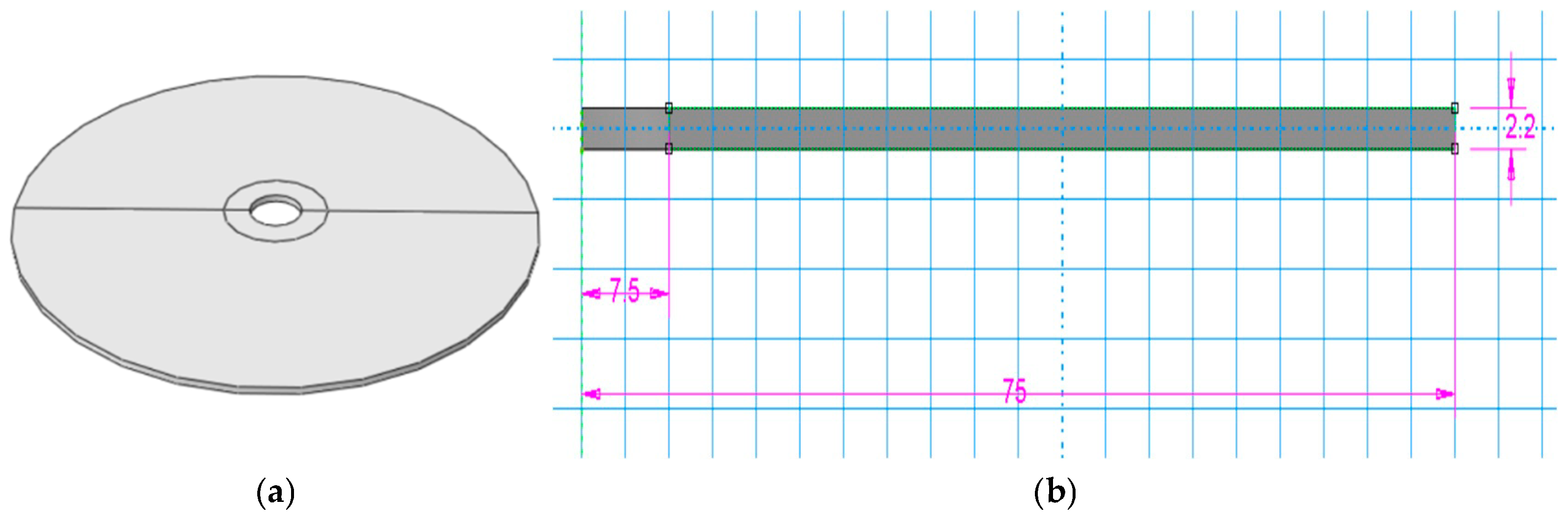
In this study, the blank for the spinning simulation of the double-conical cylindrical part is a ring-shaped plate, as shown in Figure 3. The dimensional parameters of its profile are: inner diameter D_in = 15 mm, outer diameter D_out = 150 mm, and thickness E = 2.2 mm.

Figure 3. Blank Simulation Model. (a) Blank model for simulation. (b) Dimensional parameters of the blank simulation model.

• Establishment of the Roller Simulation Model

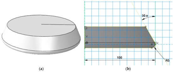
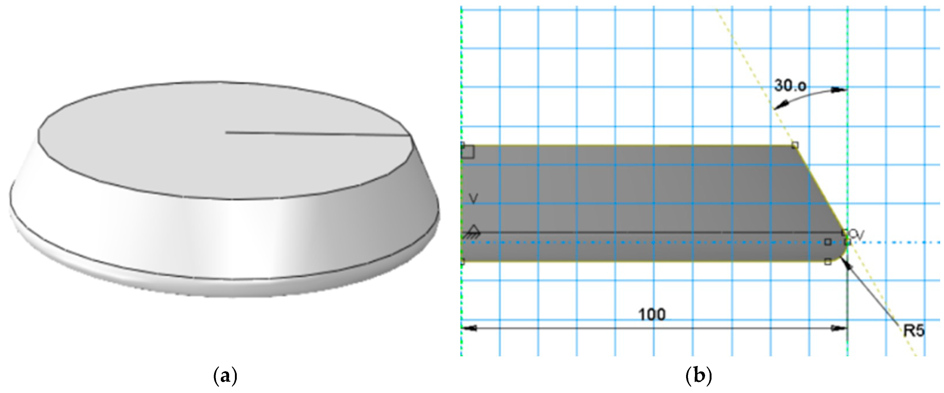
During the simulation of the strong spinning of double-cone cylindrical parts, an $\mathsf{\alpha }$-type roller is used as the spinning roller. The structural parameters of its profile surface include the roller working angle $\mathsf{\alpha }$, the roller fillet radius R, and the roller diameter D. Figure 4a shows the simulation model of the profile roller, and the parameters of the simulation model established in Figure 4b are: $\mathsf{\alpha }$ = 30°, R = 5 mm, and D = 200 mm.

Figure 4. Simulation Model of Type $\mathsf{\alpha }$ Roller. (a) Profiled Roller Simulation Model. (b) Simulation Model Parameters.

• Model Assembly

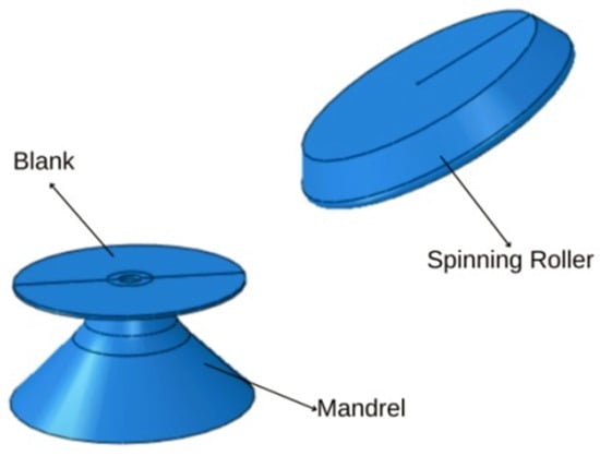
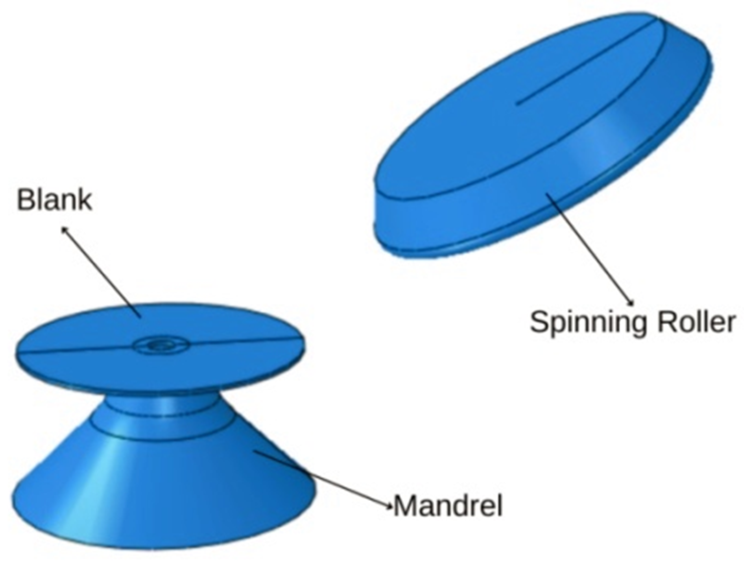
The spinning simulation analysis of the aluminum alloy double-cone cylindrical part is first carried out in Abaqus software. The model components include the spinning roller, the blank, and the mandrel. The assembled simulation model is shown in Figure 5.

Figure 5. Schematic Diagram of the Finite Element Simulation Model of the Aluminum Alloy Double Cone Spinning Part.

2.

Mesh Generation for Simulation and Solver Configuration

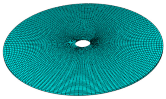
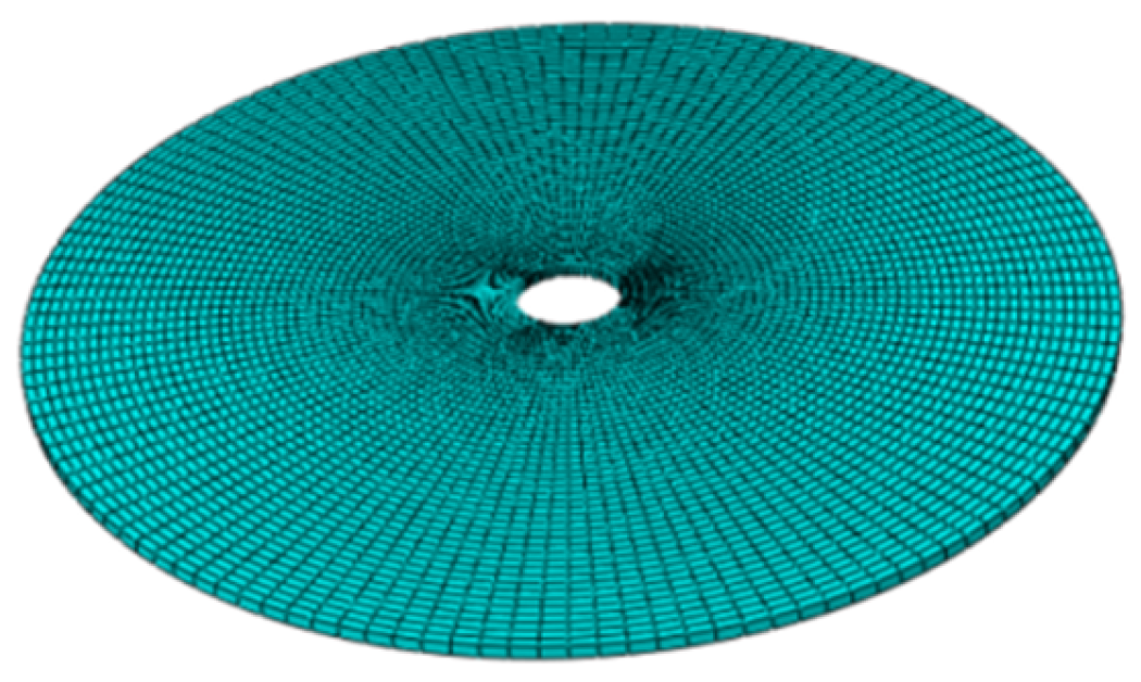
In the spinning simulation of the double-cone cylindrical part, the circular blank is meshed using C3D8R hexahedral elements. Seeds are distributed in the circumferential, radial, and axial directions. The final computational model consists of 5850 elements and 11,960 nodes. To improve computational accuracy, mesh adaptivity is applied to optimize the mesh density on the outer surface of the blank. Since the roller and the mandrel are defined as analytical rigid bodies, meshing is not required for them. The mesh generation of the circular blank is shown in Figure 6.

Figure 6. Mesh Generation of the Circular Blank.

3.

Contact Interaction and Boundary Condition Settings

In the finite element simulation of the double-conical spinning process, two primary contact interactions are involved: one between the outer surface of the roller and the upper surface of the blank, and the other between the outer surface of the mandrel and the lower surface of the blank. In this study, both interactions are defined using a surface-to-surface contact formulation. The roller and mandrel, which possess higher stiffness, are designated as the master surfaces, while the blank surface is defined as the slave surface.

For the contact properties, the normal behavior is defined as hard contact to prevent interpenetration between contacting surfaces during the spinning process. The tangential behavior is modeled using a penalty friction formulation, where the friction coefficient between the roller and the blank is set to 0.05, and that between the mandrel and the blank is set to 0.10.

Regarding boundary conditions, the mandrel rotates at a constant angular velocity around the spindle axis, driving the blank to rotate synchronously. The roller performs radial indentation and axial feed motions along a predefined trajectory. In this study, displacement boundary conditions are primarily applied to control the roller motion. The predefined trajectory point sequence is introduced through an amplitude function, enabling accurate simulation of the roller movement under complex double-conical geometries.

4.

Simulation Material Model

The blank material used in the spinning simulation of the double-cone cylindrical part is 6061 aluminum alloy. The 6061 aluminum alloy, with good plasticity, is easy to process and possesses excellent corrosion resistance. The chemical composition of 6061 is shown in Table 1, and the material model parameters of 6061 are presented in Table 2.

Table 1. Chemical Composition of 6061 Aluminum Alloy.

Element	Mg	Si	Fe	Cu	Cr	Mn	Zn	Ti	Al
Content	0.8~1.2	0.4~0.8	≤0.7	0.15~0.4	0.04~0.35	≤0.15	≤0.25	≤0.15	Balance

Table 2. Material Model Parameters of 6061 Aluminum Alloy.

Elastic Modulus/Pa	Material Density/kg·m−3	Poisson’s Ratio	Brinell Hardness/HB
68.9 × 109	2730	0.33	95

5.

Selection of Simulation Process Parameters

To ensure consistency between the simulation process and actual machining conditions, and to guarantee the engineering applicability of the extracted roller motion trajectory, the key process parameters are determined based on the characteristics of the double-conical spinning process. These parameters mainly include the roller installation angle, roller fillet radius, spindle speed, and feed ratio.

According to prior process analysis and parameter results, the simulation parameters adopted for the double-conical spinning part in this study are specified as follows: a roller installation angle of 30°, a roller fillet radius of 5 mm, a spindle speed of n = 120 r/min, and a feed ratio of 0.4 mm/r. The detailed parameter settings are listed in Table 3.

Table 3. Process Parameters for the Spinning Simulation of Double-Conical Spinning Parts.

Types of Simulation Process Parameters	Parameters
Roller Installation Angle ${\mathsf{\alpha }}_{\mathsf{\rho }}$ (°)	25
Roller Fillet Radius ${\mathrm{r}}_{\mathsf{\rho }}$ (mm)	6
Spindle Speed n (r/min)	120
Feed Ratio $\mathrm{f}$ (mm/r)	0.4

Through the aforementioned modeling procedures, contact definitions, material property assignments, and process parameter configurations, a finite element simulation model consistent with the actual double-conical spinning process is established. This provides a reliable foundation for subsequent roller trajectory extraction and virtual-real mapping.

2.2. Extraction and Transformation of Roller Simulation Trajectory Coordinates

2.2.1. Roller Trajectory Coordinate Extraction Based on ABAQUS Secondary Development

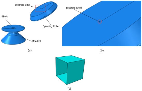
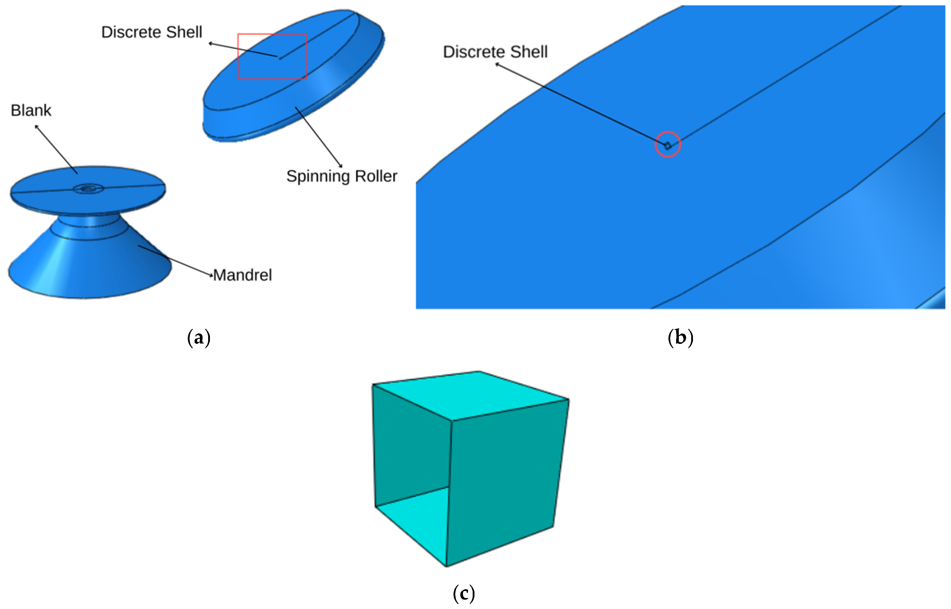
In ABAQUS, the roller is typically modeled as an analytical rigid body. Although this approach improves computational efficiency, it does not allow direct output of the continuous motion trajectory of its geometric center during post-processing. To overcome this limitation, an indirect extraction method based on a discretized shell binding strategy is adopted in this study to obtain the roller center trajectory.

Specifically, a discrete shell with dimensions of 1 mm × 1 mm × 1 mm is attached to the roller surface and constrained to move rigidly with the roller through a tie constraint, as shown in Figure 7. Acting as a motion carrier, the nodal coordinates of the discrete shell can be output frame by frame during the analysis steps, thereby indirectly representing the motion trajectory of the roller.

Figure 7. Simulation Setup for Aluminum Alloy Double-Conical Spinning Part. (a) The spinning simulation assembly of the double-conical spinning part. (b) Local magnification. (c) Discrete shell.

The side length of the discrete shell is set to 1 mm based on the following considerations. First, this size is relatively small compared to the overall geometric scale of the roller, resulting in minimal disturbance to the original contact conditions and motion state. Second, it avoids the introduction of significant geometric deviation that may arise from an excessively large size, as well as the difficulty in node identification and increased post-processing complexity associated with an excessively small size. Therefore, this dimension achieves a good balance between extraction accuracy and computational efficiency.

During the analysis step, the nodal coordinate variable (COORD) is selected as the field output. After the simulation is completed, secondary development of the Odb file is performed using a Python 3.13 script to extract the nodal coordinates of the discrete shell frame by frame, thereby obtaining discrete time-series data. The code snippet and its annotations are shown in Table 4.

Table 4. Code Snippet for Extracting Discrete Shell Node Coordinates.

Code and Comments

# Iterate through each frame in the analysis step for frame in step.frames:     # Obtain the field output named ‘COORD’ from the current frame and limit it to the subset on the specified instance.     coord = frame.fieldOutputs[‘COORD’].getSubset(region = instance)     # Retrieve the collection of field values, i.e., the coordinate information of all nodes at the current time step.     fieldValues = coord.values     # Write the node coordinates of the current frame to the file     with open(‘./all_frames_node_coord_data.txt’, ‘a’) as fp1:         for v in fieldValues:             # For each node, write the frame number, node label, and three coordinate values into the text file, separated by commas and retaining six decimal places.             fp1.write(‘%d,%d,%.6f,%.6f,%.6f\n’ %(                 frame.frameValue, v.nodeLabel,                 v.dataDouble[0], v.dataDouble[1], v.dataDouble[2]))     # Print information to the console     print(‘\nFrame: %d’ % frame.frameValue) # Output the current frame number     for v in fieldValues:         # For each node, print the node label and its coordinate values, with the coordinate values retained to six decimal places.         print(‘Node label: %d, Coord: (%.6f, %.6f, %.6f)’ % (             v.nodeLabel, v.dataDouble[0], v.dataDouble[1], v.dataDouble[2]))

This script is mainly used to extract the three-dimensional coordinate data of all nodes on the discrete shell frame by frame during the ABAQUS spinning simulation process and save them into a text file for subsequent roller trajectory fitting and error analysis. The implementation is achieved by calling the ABAQUS ODB database interface through Python, traversing all frames in the specified analysis step, reading the coordinate field output (COORD) of each frame, and writing the node labels together with their corresponding x, y, and z coordinates into a txt file in frame sequence order.

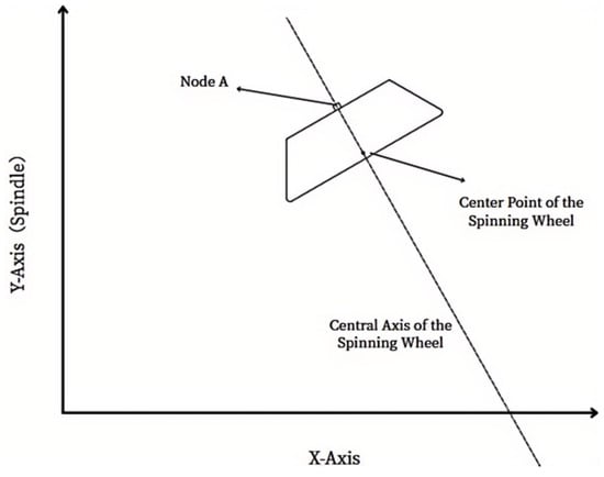
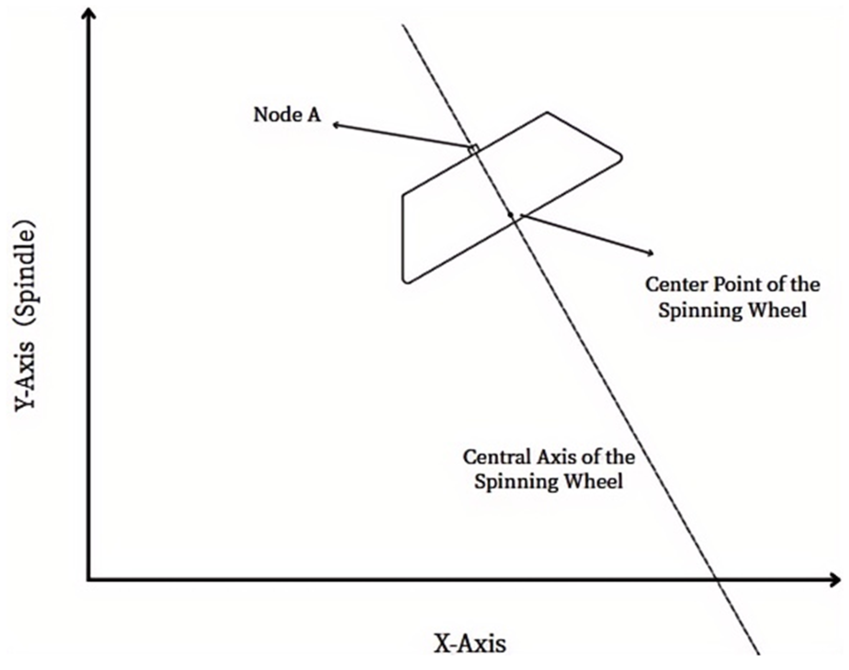
To improve the stability of trajectory extraction, a corner node of the discrete shell located along the roller installation direction is selected as the characteristic node, denoted as point A. The relative position between this node and the roller center remains constant throughout the simulation, and its geometric relationship is clearly defined, which facilitates the establishment of a stable coordinate mapping relationship. Based on this approach, the continuous motion of the roller can be transformed into a discrete coordinate sequence, providing a reliable data foundation for subsequent calculation of the roller center trajectory and its transformation to machine tool coordinates.

2.2.2. Calculation of the Roller Center Trajectory Coordinates

After completing the finite element simulation of the double-conical cylindrical part, a Python script is employed to extract the spatial coordinates of the characteristic node of the discrete shell from the Odb file at each frame. Let the coordinates of the reference node A at the i-th frame be expressed as: $A_i(x_{Ai},\hspace{0.17em}{y}_{Ai},\hspace{0.17em}{z}_{Ai})$, where $x_{Ai}$, $y_{Ai}$ and $z_{Ai}$ denote the coordinate components of node A in the global simulation coordinate system along the three directions.

To further determine the coordinates of the roller center point $P_i$, it is necessary to establish a fixed geometric relationship between the discrete shell and the roller. Let the side length of the discrete shell be $\mathrm{a}$, the roller thickness be $\mathrm{d}$, and the roller installation angle be $\theta$. The fixed offsets of the roller center relative to the reference node of the discrete shell are denoted as $\Delta x$, $\Delta y$, and $\Delta z$, respectively.

Since the discrete shell and the roller are constrained to move synchronously through a tie constraint, the relative position between node A and the roller center point P remains constant throughout the simulation. Therefore, the following relationship can be established:

$$P_i(x_{Pi},\hspace{0.17em}{y}_{Pi},\hspace{0.17em}{z}_{Pi})=A_i(x_{Ai},\hspace{0.17em}{y}_{Ai},\hspace{0.17em}{z}_{Ai})+(\Delta x,\Delta y,\Delta z)$$

(1)

According to the geometric relationship illustrated in Figure 8, the offset of the roller center relative to the reference node can be determined by the side length of the discrete shell, the roller thickness, and the installation angle.

Figure 8. Schematic Diagram of the Roller Position in the Coordinate System of the Spinning Simulation for the Double-Conical Spun Part.

If the discrete shell is regarded as an auxiliary rigid marker attached to the roller surface, its center position relative to the reference node can be expressed as:

$$\Delta x={\displaystyle \frac{a}{2}}+{\displaystyle \frac{d}{2}}\mathit{cos}\theta$$

(2)

$$\Delta y={\displaystyle \frac{a}{2}}$$

(3)

$$\Delta z={\displaystyle \frac{d}{2}}\mathit{sin}\theta +h$$

(4)

In the above expressions, h represents the additional geometric offset of the roller center relative to the contact reference surface of the discrete shell, which characterizes the fixed distance between the roller center and the large-end circular surface.

By substituting Equations (2)–(4) into Equation (1), the coordinates of the roller center point at the i-th frame can be expressed as:

$$x_{Pi}=x_{Ai}+{\displaystyle \frac{a}{2}}+{\displaystyle \frac{d}{2}}\mathit{cos}\theta$$

(5)

$$y_{Pi}=y_{Ai}+{\displaystyle \frac{a}{2}}$$

(6)

$$z_{Pi}=z_{Ai}+{\displaystyle \frac{d}{2}}\mathit{sin}\theta +h$$

(7)

In this study, the side length of the discrete shell is set to $a=1$ mm, the roller thickness is $d=30$ mm, and the roller installation angle is $\theta =30^{\circ }$. By substituting the extracted coordinates of node A at each frame into Equations (5)–(7), the coordinates of the roller center point $P_1$ can be obtained as: $(x_A+13.433,y_A-22.267,z_A+0.5)$.

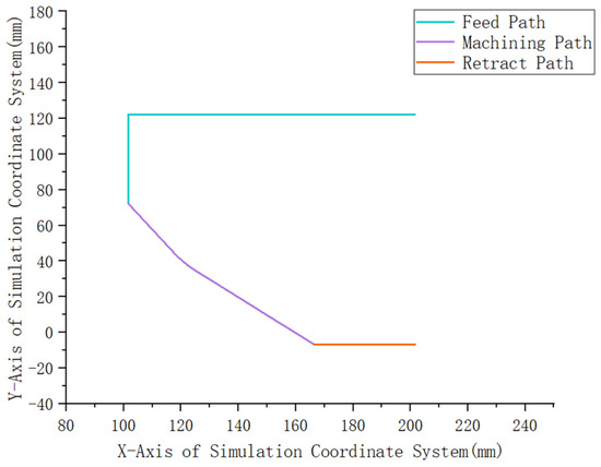
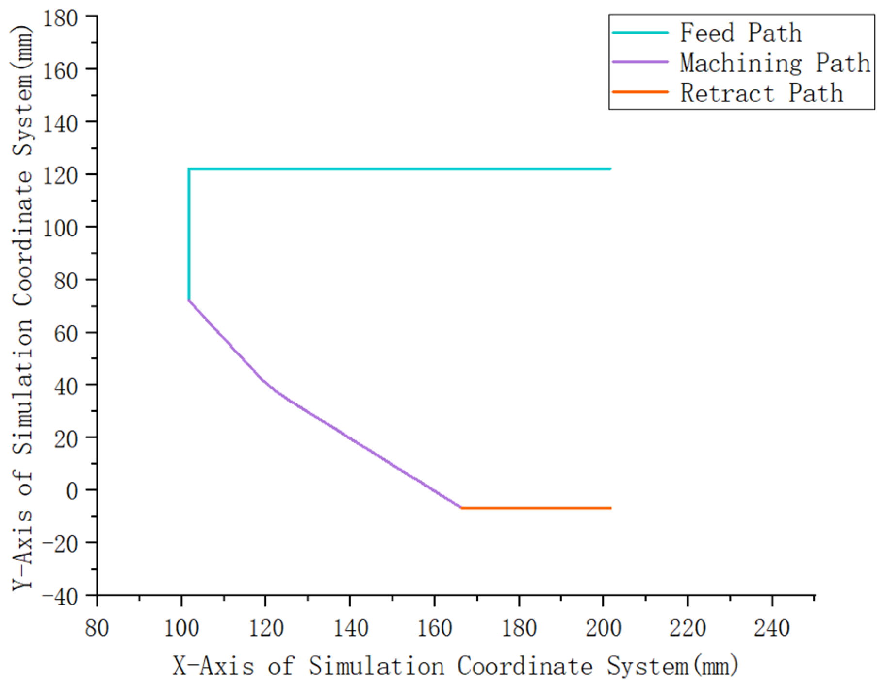
Subsequently, the coordinates of node A at each frame are substituted into Equation (1) to calculate the corresponding coordinates of the roller center point $P_1$ for all frames. By organizing the resulting coordinate data, the simulated motion trajectory of the roller for the double-conical spinning part can be obtained. The extracted trajectory is illustrated in Figure 9.

Figure 9. Roller Center Motion Trajectory in the Simulation Coordinate System.

2.2.3. Trajectory Coordinate Transformation

After extracting the simulated roller motion trajectory, the obtained trajectory data remain in the ABAQUS simulation coordinate system and cannot be directly applied to machine tool execution. To enable the practical implementation of the simulated trajectory, it is necessary to establish a mapping relationship between the simulation coordinate system and the machine tool coordinate system.

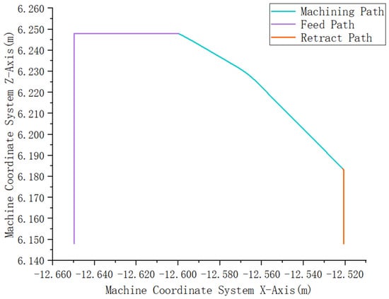
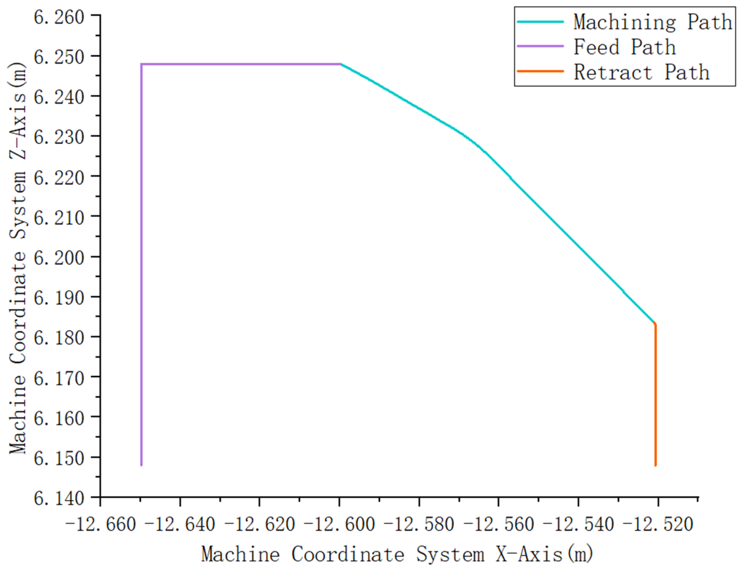
By analyzing the spatial relationship between the two coordinate systems and considering the actual machine structure and motion directions, coordinate transformation is performed on the simulated trajectory data. This includes aligning the coordinate origins and adjusting the spatial positions to ensure consistency with the machine tool coordinate representation and motion constraints. The trajectory data are listed in Table 5, and the corresponding trajectory is shown in Figure 10.

Table 5. Transformed Roller Trajectory Coordinate Data (see Supplementary Materials, Table S1 for details).

Number of Data Points (n)	X Coordinates	Y Coordinates	Z Coordinates
1	−12.6498	0.05	6.148
2	−12.6498	0.05	6.149
3	−12.6498	0.05	6.15
4	−12.6498	0.05	6.151
$⋮$	$⋮$		$⋮$
401	−12.5208	0.05	6.084

Figure 10. Roller Trajectory in the Machine Tool Coordinate System.

To meet the requirements of numerical control (NC) machine tools for interpolation based on incremental displacement, the original coordinate trajectory is transformed into displacement increments between adjacent points using first-order differencing, as shown in Table 6.

Table 6. Processed Roller Trajectory Coordinates (see Supplementary Materials, Table S2 for details).

Number of Data Points (n)	X Coordinates	Y Coordinates	Z Coordinates
1	0	0	0
2	0	0	1
3	0	0	2
4	0	0	3
$⋮$	$⋮$		$⋮$
401	129	0	−64

Based on the proposed discrete shell binding and coordinate transformation methods, accurate extraction of the roller motion trajectory is achieved, transforming the continuous simulation process into a discrete spatiotemporal coordinate sequence. This trajectory dataset provides a high-fidelity data foundation for G-code generation and effectively resolves the mismatch in data representation between simulation results and actual machine tool execution.

3. Extraction of Roller Motion Trajectory from Spinning Equipment

3.1. Construction of Roller Trajectory Acquisition and Visualization System

To obtain the actual motion trajectory of the roller during the spinning process, a trajectory acquisition and visualization system based on displacement sensors is developed in this study to measure and record the spatial position of the roller during machining. The system consists of a displacement sensor and a virtual-real mapping system.

The roller feed is a key parameter affecting the quality and efficiency of the spinning process, and its accurate measurement is of great importance. Although spinning machines are typically equipped with high-precision built-in sensors, differences in communication protocols across various machines make data acquisition difficult. To ensure the generality and portability of the virtual-real mapping system, an external sensor solution is adopted using a non-intrusive deployment approach.

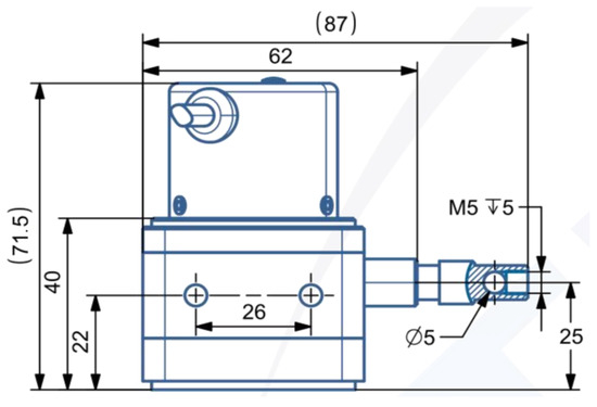
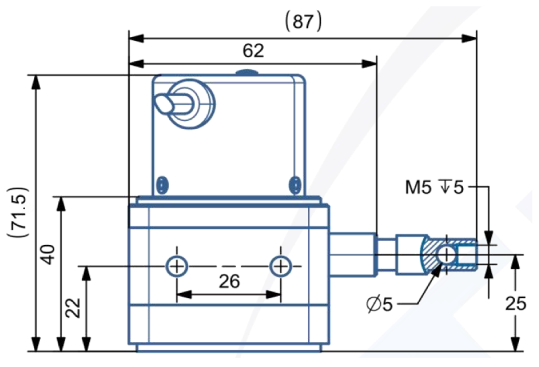
Based on a comprehensive analysis of application requirements, an absolute draw-wire displacement sensor with an RS485 output signal and a resolution of 1024 is selected. The sensor has a measurement range of 1000 mm, which meets the measurement requirements, and a displacement resolution of 0.098 mm, satisfying accuracy demands. It features a linear accuracy of ±0.1% and a repeatability accuracy of ±0.01%, ensuring high-precision measurement. With a protection rating of IP54 and explosion-proof capability, the sensor is suitable for complex industrial environments. In addition, its compact size facilitates installation, fully meeting practical deployment requirements. The dimensional parameters of the sensor are shown in Figure 11.

Figure 11. Dimensional Parameters of the Displacement Sensor.

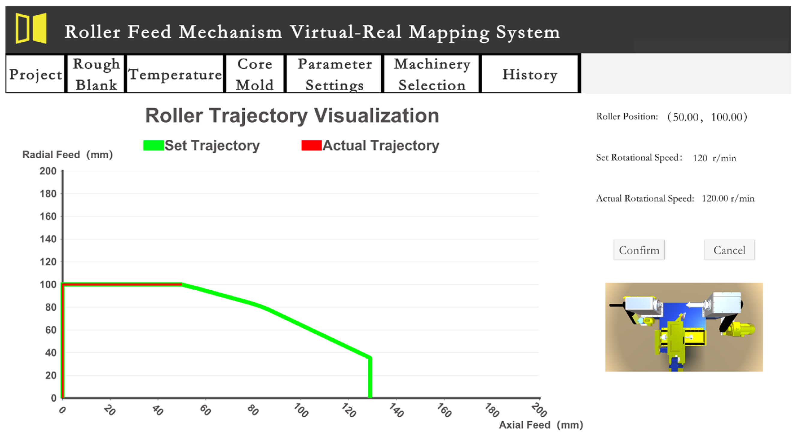
To enable real-time monitoring of the roller motion trajectory, a virtual-real mapping system is developed based on the Unity3D 2022.3019f1c1 platform. The sensor is connected to the system via a USB interface, and data transmission is achieved using the Modbus-RTU communication protocol. The acquired displacement data are processed and visualized using the XChart plugin, enabling real-time monitoring of the roller motion trajectory.

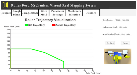
As shown in Figure 12, the visualization of the roller trajectory consists of two components: the prescribed trajectory generated by finite element simulation (green curve), and the actual measured trajectory of the roller (red curve).

Figure 12. Visualization of Roller Trajectories.

3.2. Roller Trajectory Extraction and Fitting

• Sensor Measurement Position Zeroing

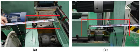
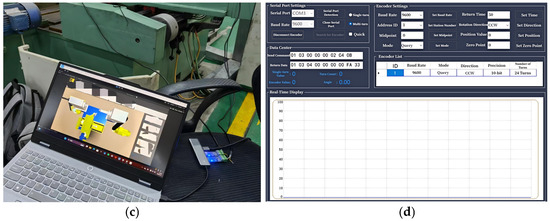
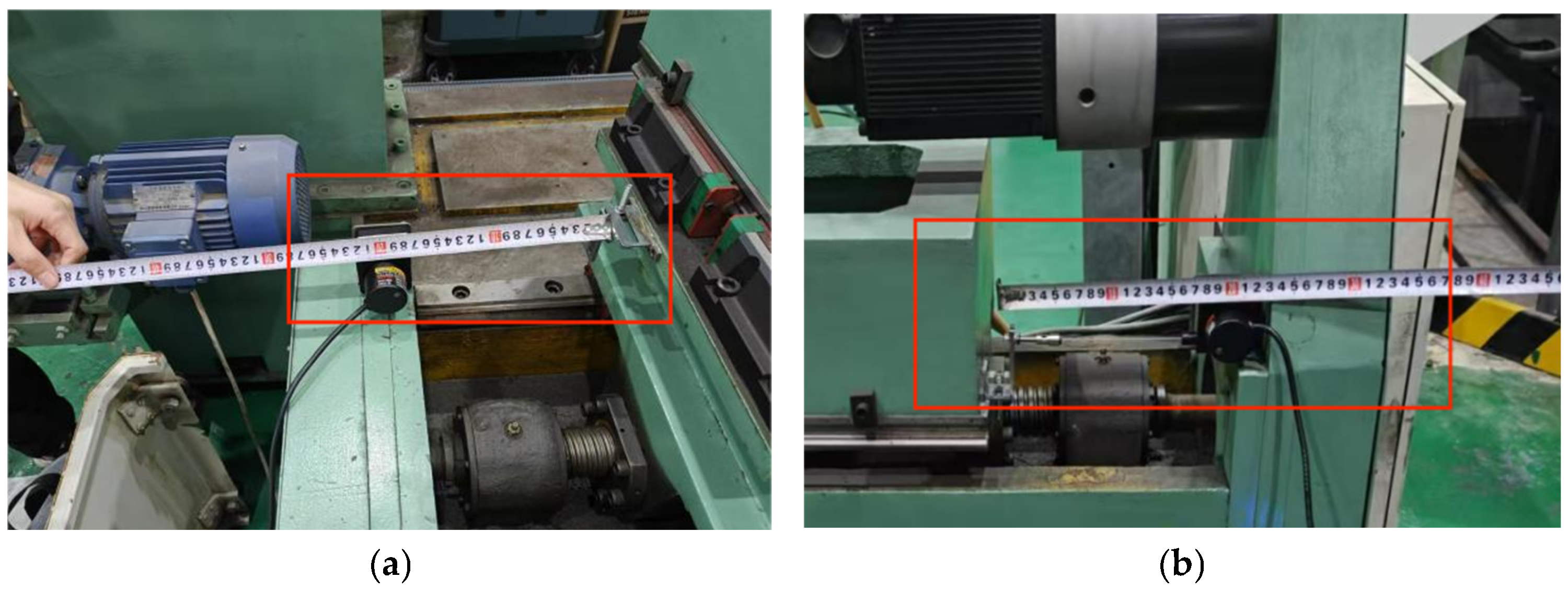
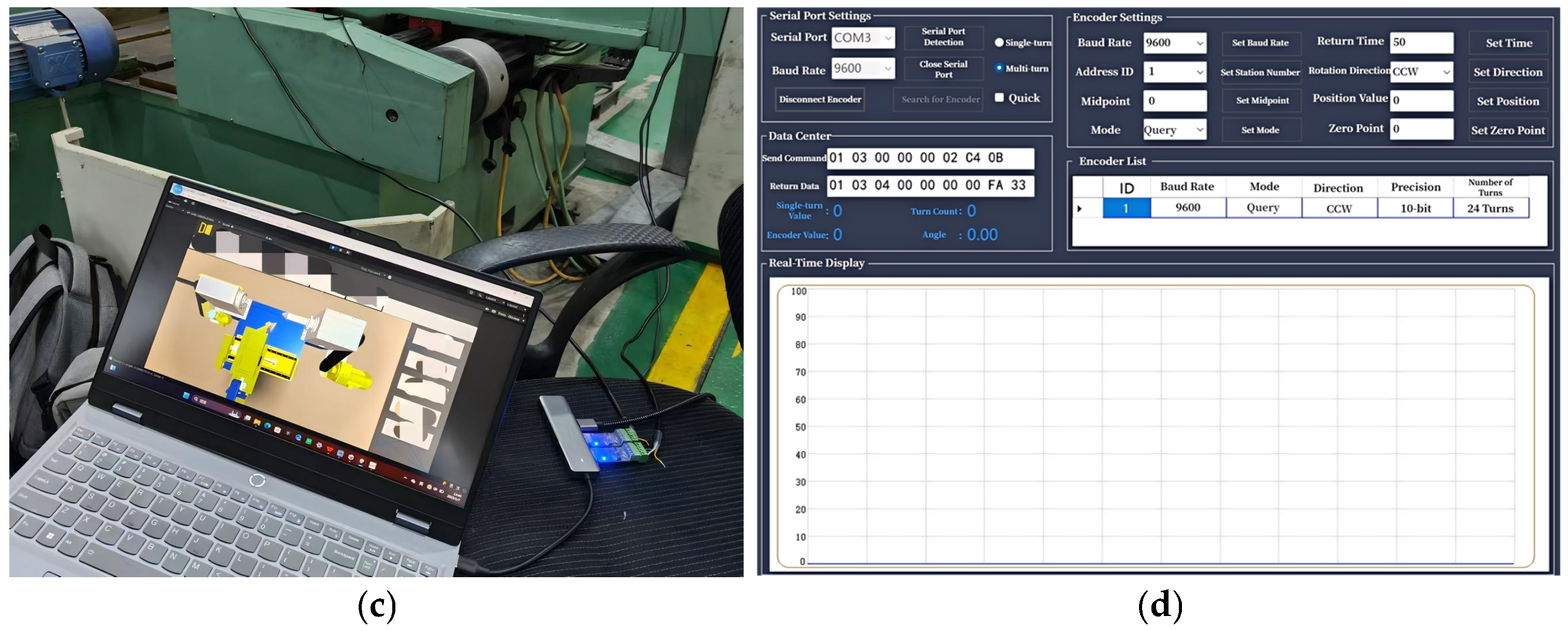
Due to the need for a certain amount of pre-tension when installing the draw-wire displacement sensor, the measurement position does not correspond to the zero point. Therefore, zeroing is required. The zeroing process is shown in Figure 13. First, the virtual-real mapping system is started and the sensor communication channel is opened. Then, the machine tool’s spinning wheel holder is adjusted to the zero point and the current measurement value is set as the zero point through the host computer software, ensuring that the sensor measurement aligns with the actual starting coordinates of the machine tool.

Figure 13. Draw-Wire Sensor Measurement Position Zeroing. (a) Initial Position in the X Direction. (b) Initial Position in the Z Direction. (c) Sensor Receiving Position Information. (d) Sensor Measurement Position Zeroing.

2.

Experimental Verification of Spinning Roller Trajectory Fitting

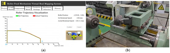
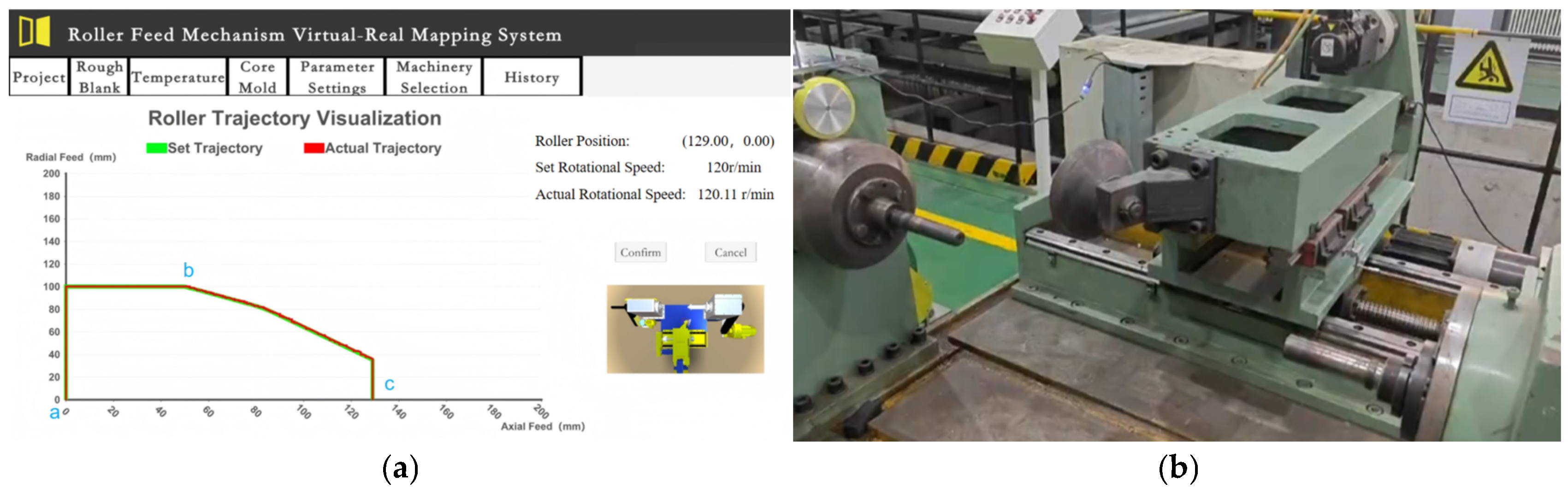
After zeroing, the virtual-real mapping system is used to verify the rationality of the extracted trajectory, ensuring its applicability to the single-roller spinning machine. Once the verification is complete, the extracted roller simulation trajectory is entered into the CNC system of the spinning machine. The roller trajectory fitting experiment is then initiated. In the experiment, the roller’s motion trajectory is divided into three key points: point a, point b, and point c. The following analysis is conducted for each of these points.

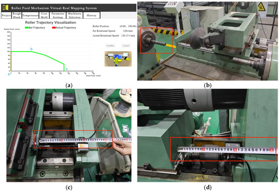
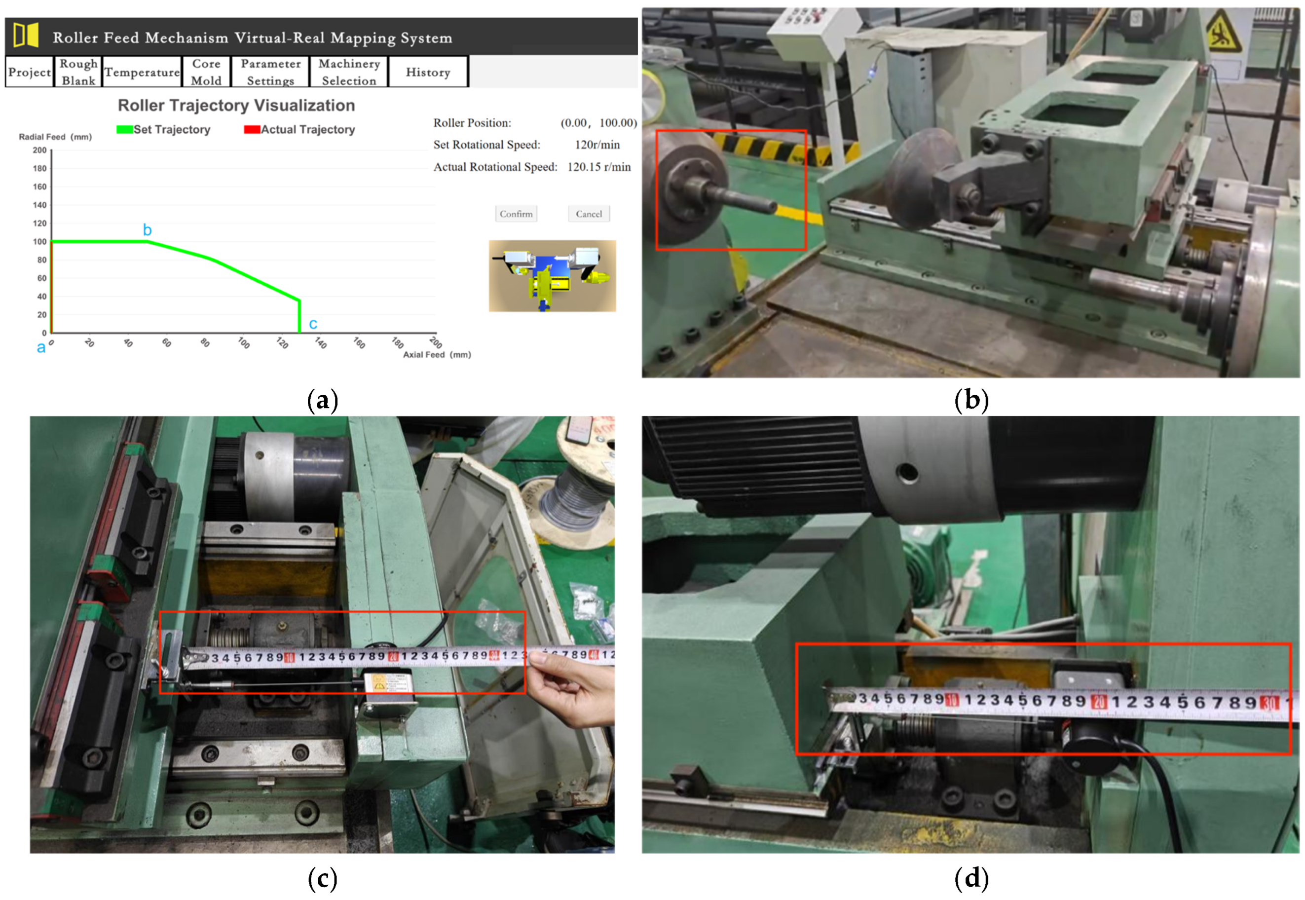
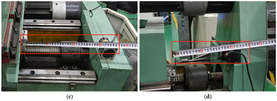
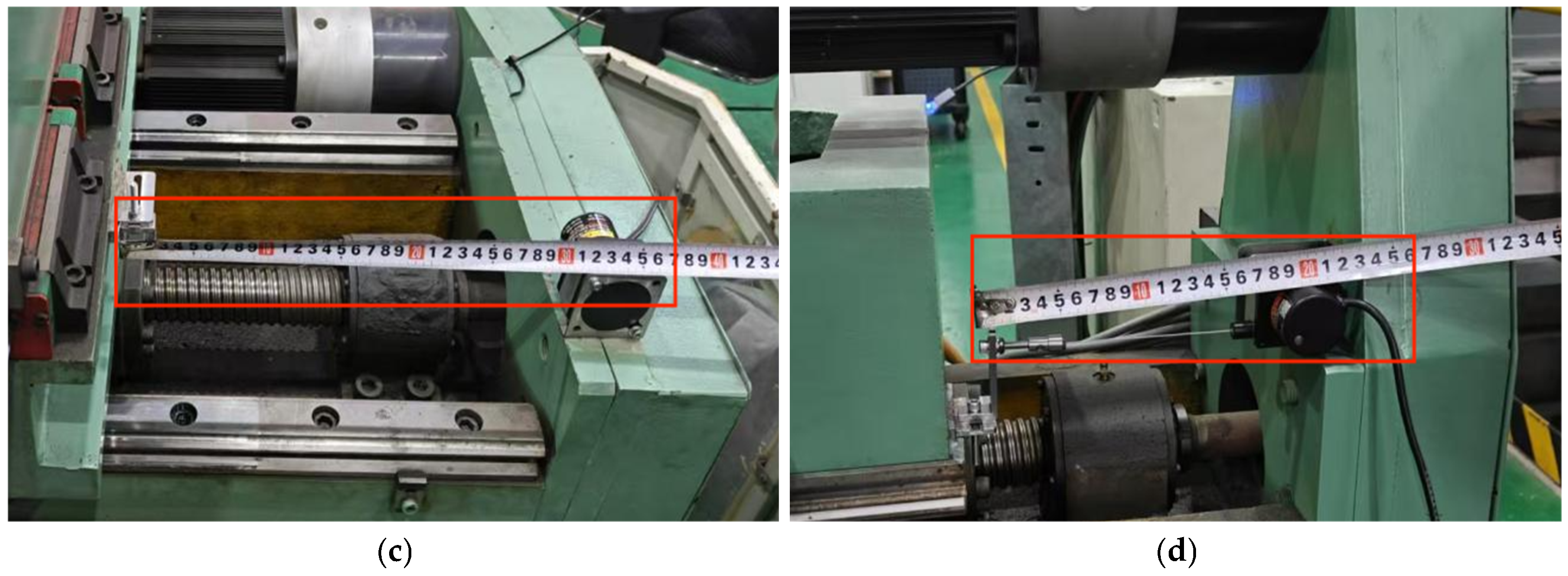
• Point A is the starting point of the machine tool coordinate system and also the initial position of the roller. As shown in Figure 14, (a) is the virtual-real mapping visualization interface, and (b) is the corresponding position of the actual spinning machine. Since this study only focuses on trajectory fitting experiments, the figure does not include the part (the red frame in the figure serves as a scale and is not a part). (c) and (d) represent the axial and radial coordinates of the roller’s initial position, respectively.

Figure 14. Trajectory Fitting Position a. (a) Virtual-Real Mapping Visualization Interface. (b) Actual Position of the Spinning Machine. (c) Axial Coordinate of the Spindle. (d) Radial Coordinate of the Spindle.

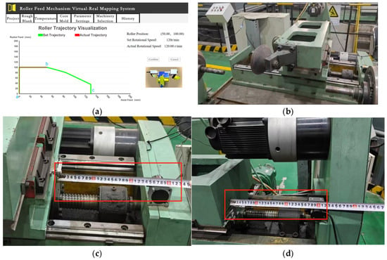
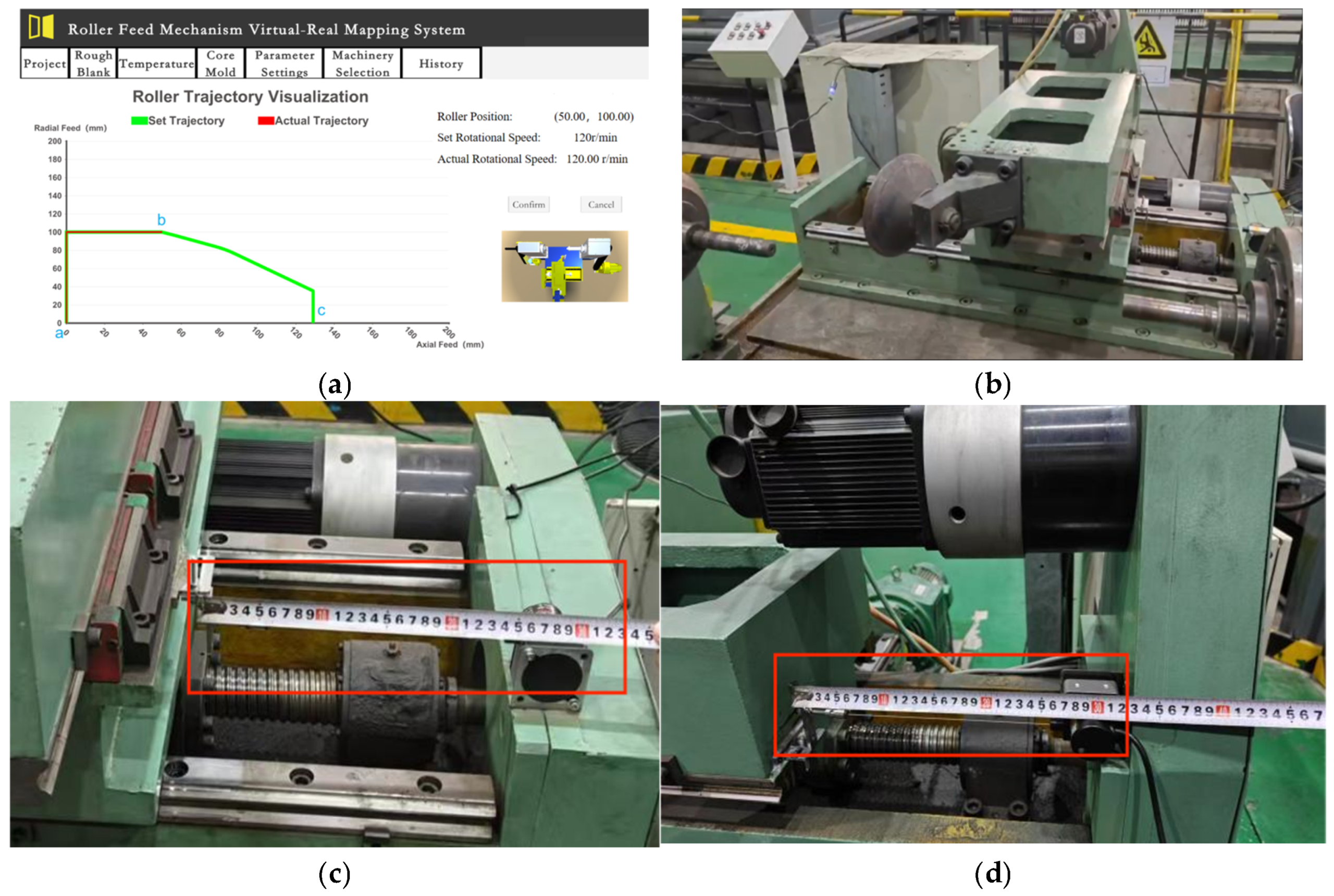
• The spindle moves to point b, completing the trajectory fitting of the simulation path segment ab, and the spinning machine completes the axial feed. As shown in Figure 15, (a) is the visualization interface of the virtual simulation model running to point b, (b) is the corresponding position of the actual spinning machine, and (c) and (d) are the axial and radial coordinates of the spindle, respectively. From the trajectory fitting curve in (a), it can be seen that the fitting results are good.

Figure 15. Trajectory Fitting Position b. (a) Virtual simulation model running to point b. (b) Spinning machine running to point b. (c) Axial coordinate at point b. (d) Radial coordinate at point b.

• The roller moves to point c, completing the trajectory fitting for the bc segment. The spinning machine completes the spinning process and performs the tool withdrawal action. As shown in Figure 16, (a) shows the visualization of the virtual simulation model running to point c, (b) shows the corresponding position of the actual spinning machine, and (c) and (d) show the axial and radial coordinates of the roller, respectively. From the trajectory fitting curve in (a), it can be seen that the fitting results are good, but there is some error.

Figure 16. Trajectory Fitting at Position c. (a) Virtual simulation model running to point c. (b) Spinning machine running to point c. (c) Axial coordinates at point c. (d) Radial coordinates at point c.

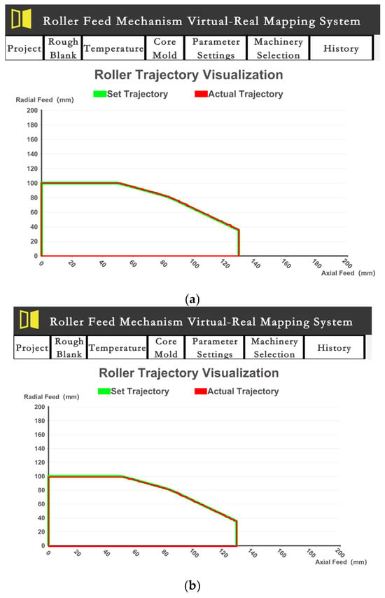
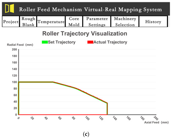
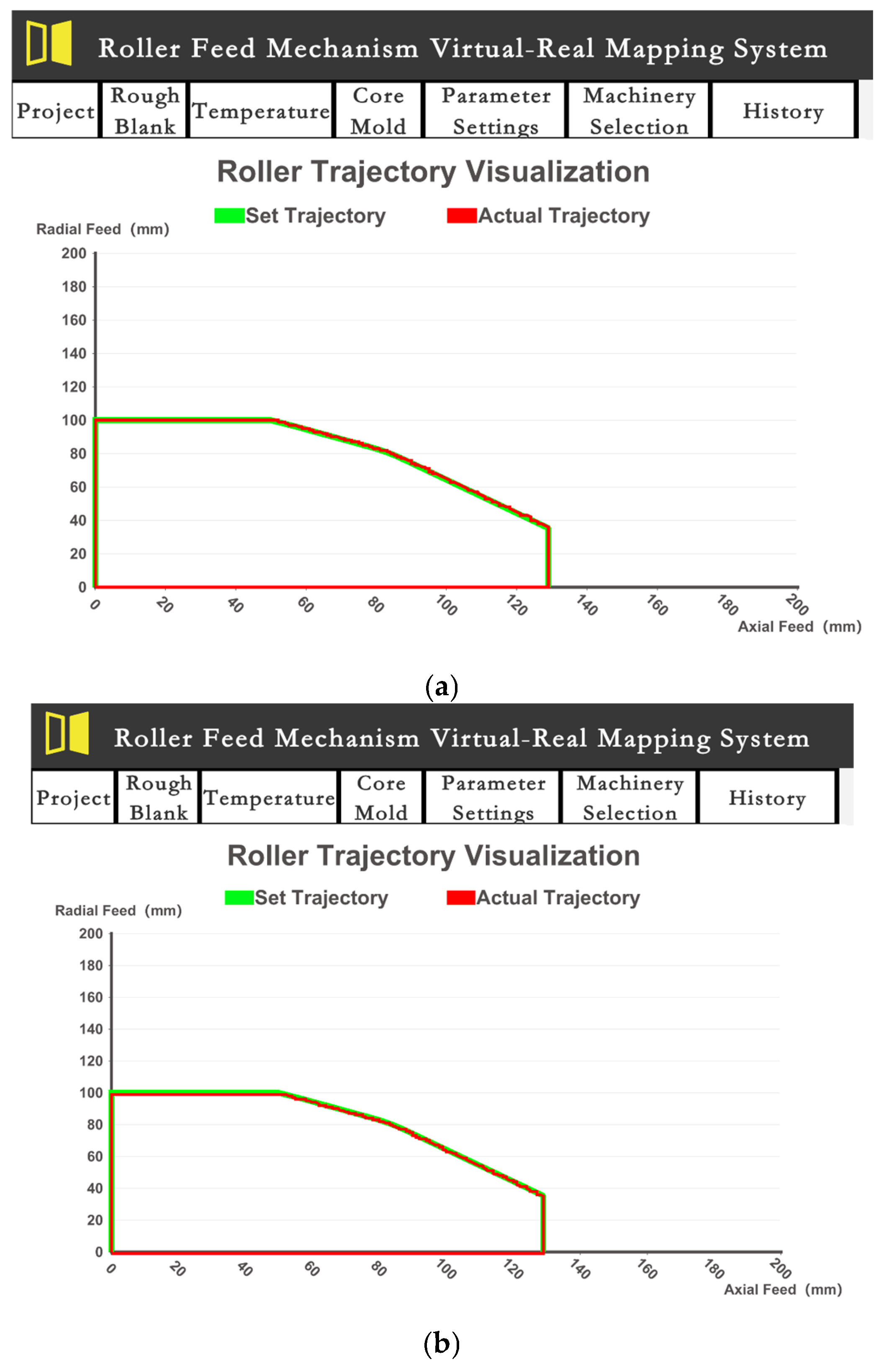
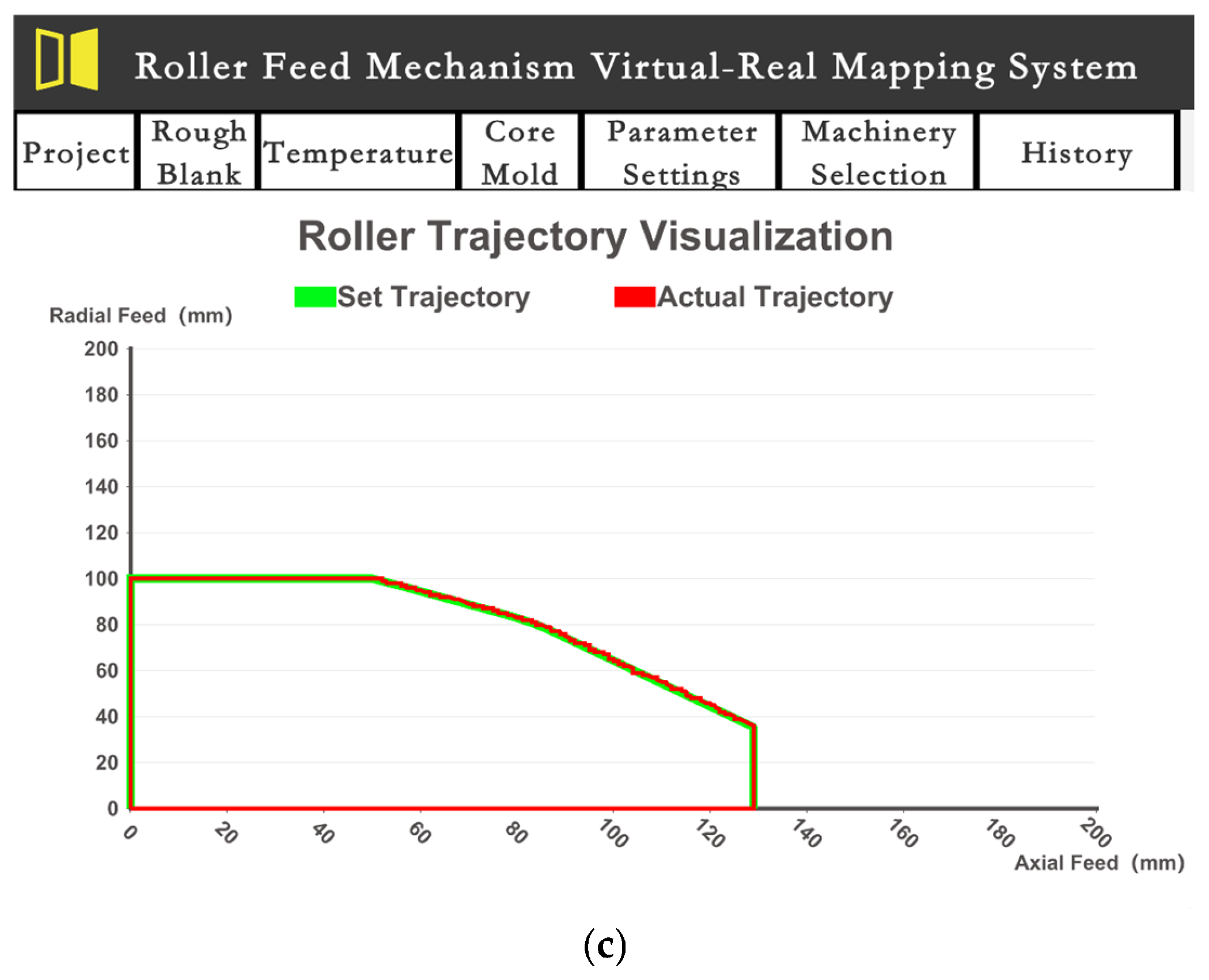
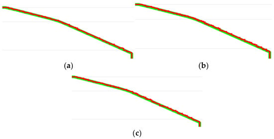
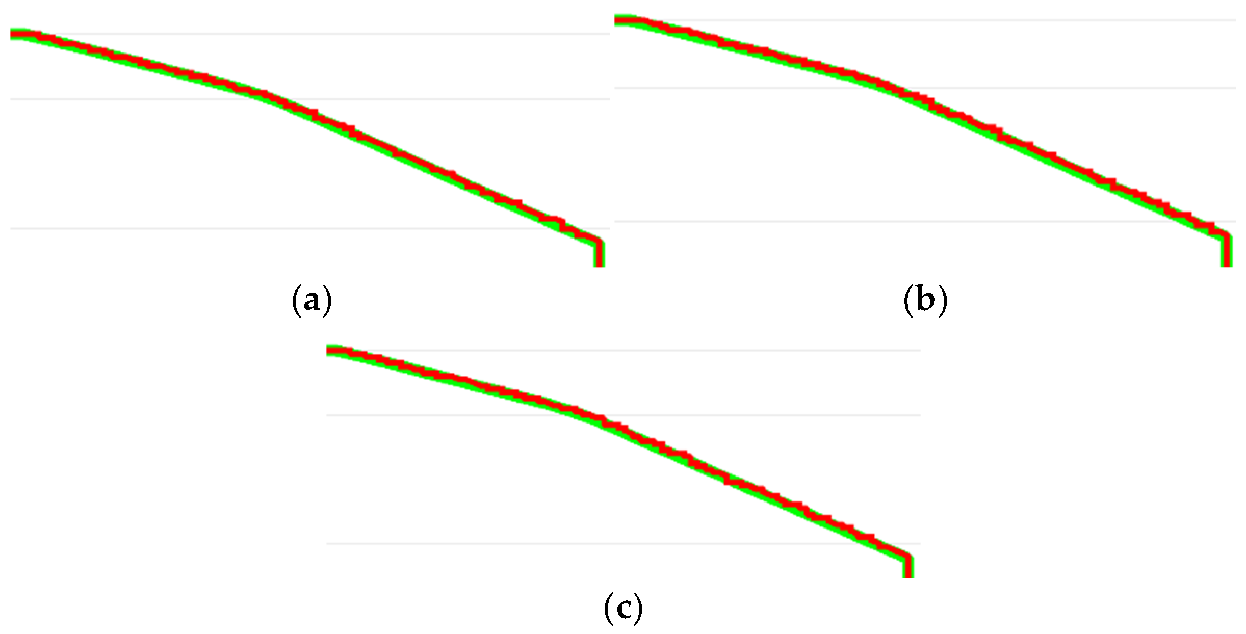
The above operation is repeated for a total of three trajectory fitting experimentals, and the fitting results are shown in Figure 17.

Figure 17. Trajectory Fitting Visualization Curves. (a) First Set of Trajectory Fitting experimental. (b) Second Set of Trajectory Fitting experimental. (c) Third Set of Trajectory Fitting experimental.

3.3. Quantitative Analysis of Trajectory Fitting Deviations

As shown in Figure 17, the roller trajectory in the linear section has been fully fitted, and the conical section trajectory also shows good fitting results, although some errors remain. To further analyze the characteristics of the conical section trajectory, a local zoomed-in view is provided in Figure 18. The enlarged figure reveals that the actual movement trajectory of the roller exhibits a distinct stepped pattern, while the simulated trajectory appears as a smooth curve. Due to the significant difference in their representations, it is difficult to directly compare the errors between the two.

Figure 18. Enlarged View of Fitted Trajectory Curves in the Conical Section. (a) Enlarged View of the First Set of Fitted Trajectories. (b) Enlarged View of the Second Set of Fitted Trajectories. (c) Enlarged View of the Third Set of Fitted Trajectories.

Therefore, this study adopts the projection method to perform the secondary fitting between the actual trajectory and the simulated trajectory, in order to achieve more accurate error analysis. The mathematical Equations and principles are as follows:

Let the actual collected data points be defined as:

$$P_i=\left(x_i,y_i\right), i=1,2,3,\dots ,n$$

(8)

Let the simulated trajectory curve be defined as:

$$C\left(u\right)=\left(x\right(u),y(u\left)\right),u\in [u_0,u_1]$$

(9)

where u denotes the arc-length parameter of the trajectory.

Then, the squared distance from each point $P_i$ to the simulated trajectory curve is:

$$D_i(u)={‖P_i-C\left(u\right)‖}^2={(x_i-x(u\left)\right)}^2+{(y_i-y(u\left)\right)}^2$$

(10)

To minimize the distance from the point to the curve, take the extremum with respect to point $u$:

$${\displaystyle \frac{{dD}_i}{du}}=2(x_i-x(u))(-x^{\prime }(u))+2(y_i-y(u))(-y^{\prime }(u))=0$$

(11)

The simplification yields:

$$(x_i-x(u\left)\right)x^{\prime }\left(u\right)+(y_i-y(u\left)\right)y^{\prime }\left(u\right)=0$$

(12)

Since the equation is nonlinear, Newton’s method is used to solve it, and the iterative equation is constructed.

Let:

$$f\left(u\right)=(x_i-x(u\left)\right)x^{\prime }\left(u\right)+(y_i-y(u\left)\right)y^{\prime }\left(u\right)$$

(13)

Its derivative is:

$$f\prime \left(u\right)=(x_i-x(u\left)\right)x^{″}\left(u\right)+(y_i-y(u\left)\right)y^{″}\left(u\right)-{\left(x^{\prime }\right(u\left)\right)}^2-{\left(y^{\prime }\right(u\left)\right)}^2$$

(14)

Newton’s method iteration Equation is:

$$u_{k+1}=u_k-{\displaystyle \frac{f\left(u_k\right)}{f^{\prime }\left(u_k\right)}}$$

(15)

Using this method, we progressively approach the projection position $u_i^{*}$ for each measurement point on the curve. Once the point $u_i^{*}$ is obtained, we calculate its coordinates on the curve as:

$$C\left(u_i^{*}\right)=\left(x\right(u_i^{*}),y(u_i^{*}\left)\right)$$

(16)

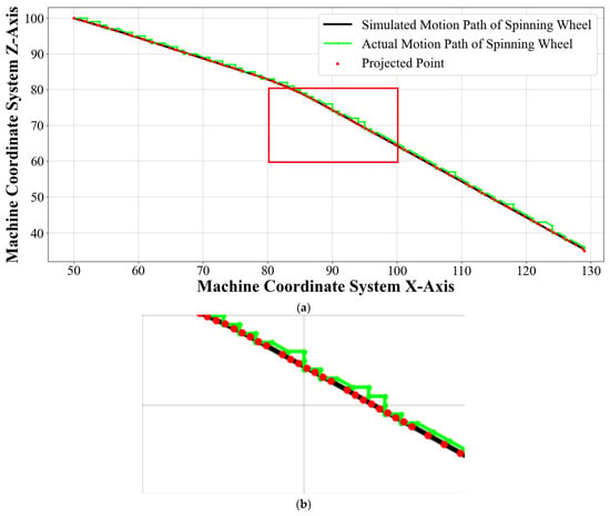
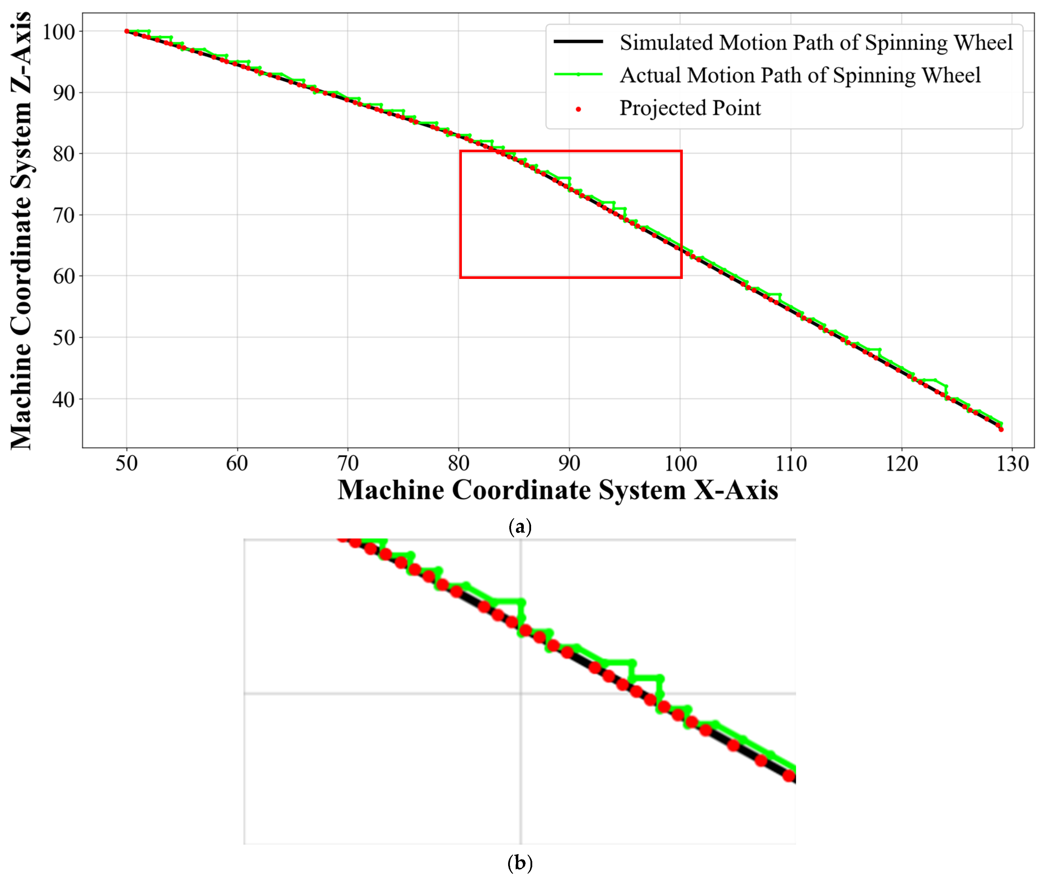
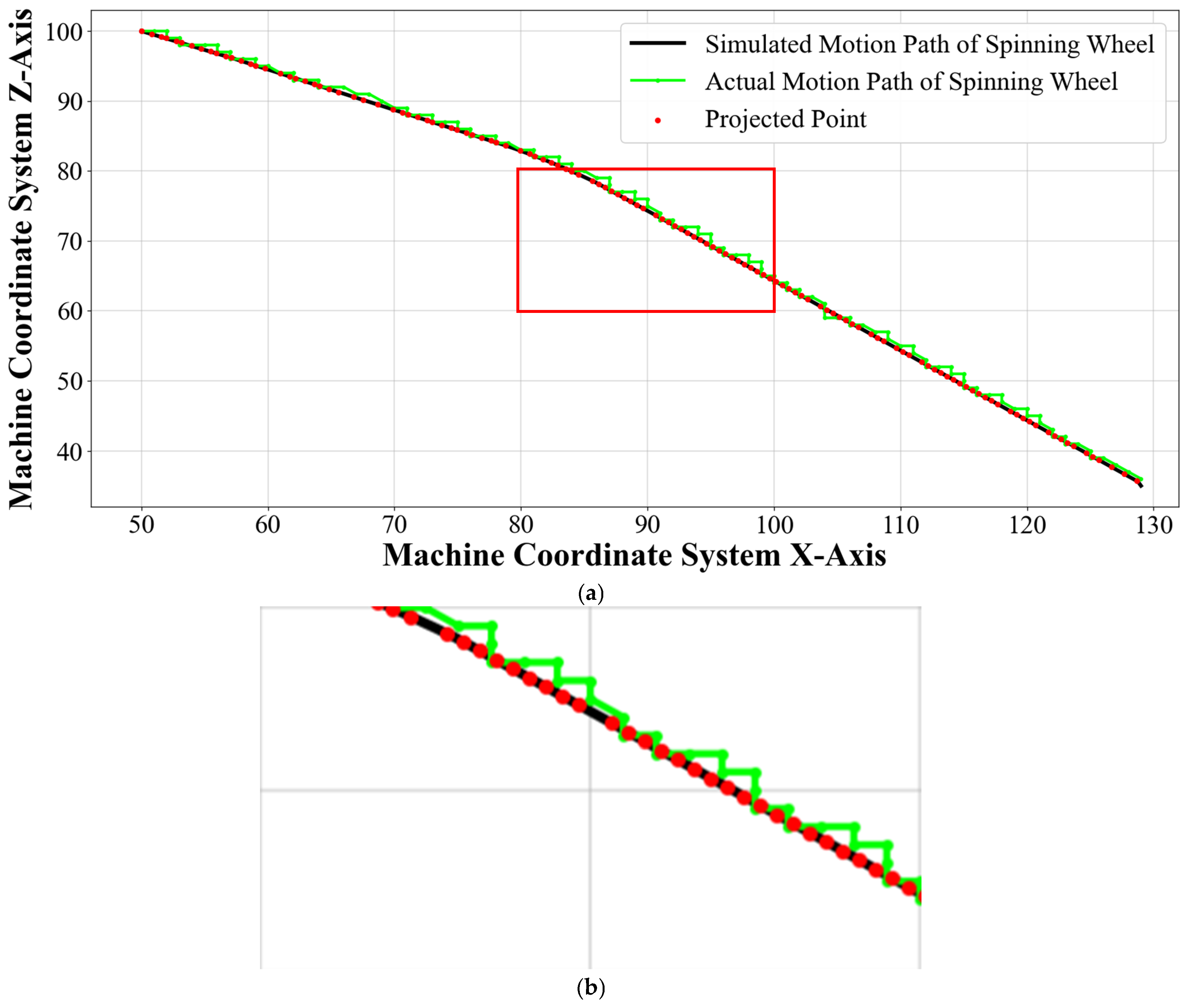
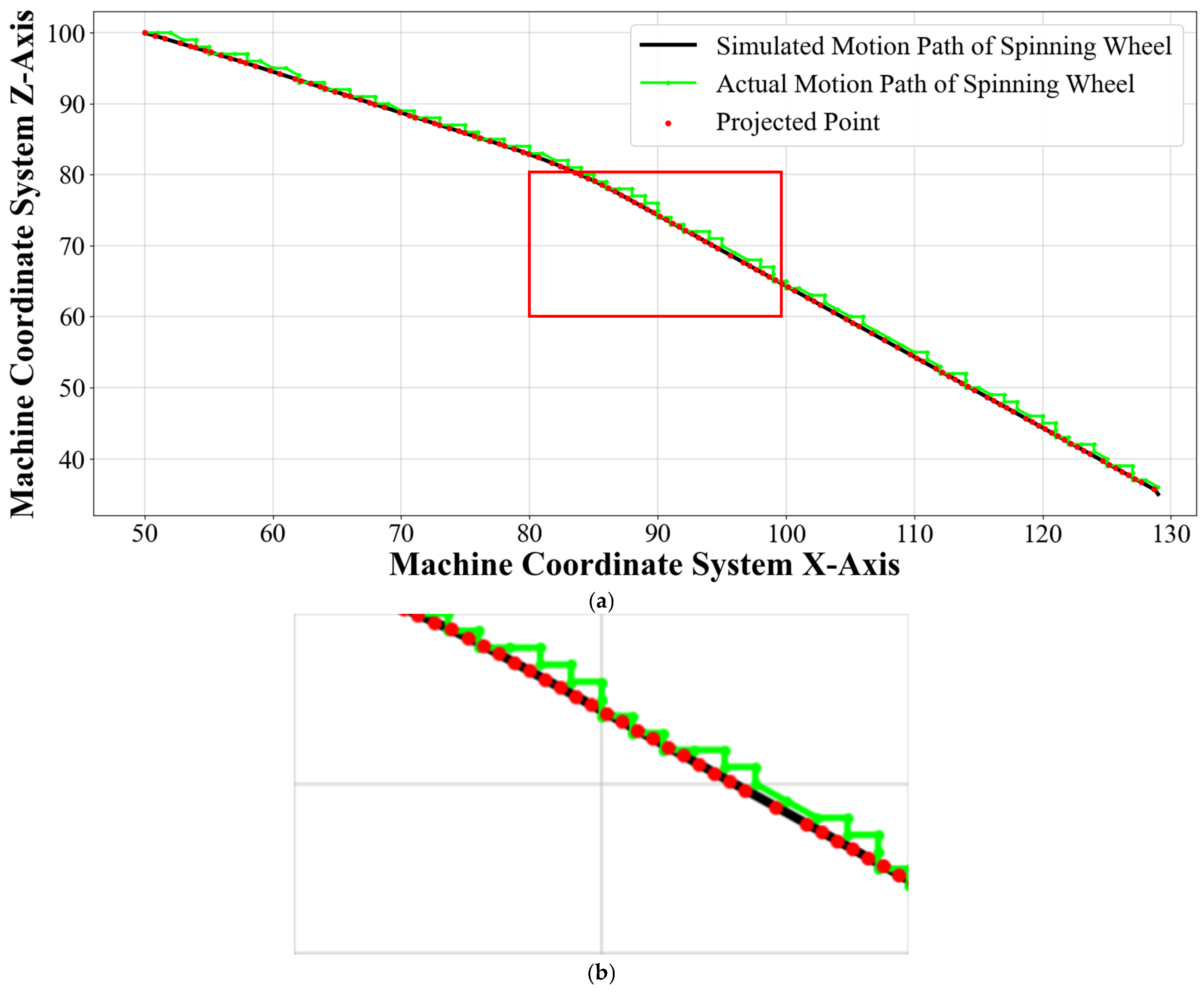
Using the method described above, the projection point trajectory coordinates for each measurement point on the roller simulation motion trajectory are calculated. Corresponding trajectory fitting images are plotted. The coordinate data and trajectory fitting images for the three sets of experiments correspond to Table 7 and Figure 19, Table 8 and Figure 20, and Table 9 and Figure 21, respectively.

Table 7. Projected Point Trajectory Coordinates for the First Set of Measurement Data (see Supplementary Materials, Table S3 for details).

Number of Data Points (n)	Measured X Coordinates	Measured Z Coordinates	Projected X Coordinates	Projected Z Coordinates
1	50.0000	100.0000	50.0000	100.0000
2	51.0000	100.0000	50.7957	99.5988
3	52.0000	100.0000	51.5820	99.1945
4	52.0000	99.0000	51.9904	98.9817
5	53.0000	99.0000	52.7709	98.5696
6	54.0000	99.0000	53.5437	98.1552
7	54.0000	98.0000	53.9613	97.9288
8	55.0000	98.0000	54.7291	97.5083
9	55.0000	97.0000	55.1522	97.2745
$⋮$	$⋮$	$⋮$	$⋮$	$⋮$
118	129.0000	35.0000	129.0000	35.0000

Figure 19. The first Group of Measurement Data. (a) Trajectory Fitting by Projection Method. (b) The First Group Locally Enlarged Drawing of Fitting Trajectory.

Table 8. Projected Point Trajectory Coordinates for the Second Set of Measurement Data (see Supplementary Materials, Table S4 for details).

Number of Data Points (n)	Measured X Coordinates	Measured Z Coordinates	Projected X Coordinates	Projected Z Coordinates
1	50.0000	100.0000	50.0000	100.0000
2	51.0000	100.0000	50.7957	99.5988
3	52.0000	100.0000	51.5820	99.1945
4	52.0000	99.0000	51.9904	98.9817
5	53.0000	99.0000	52.7709	98.5696
6	53.0000	98.0000	53.1864	98.3475
7	54.0000	98.0000	53.9613	97.9288
8	55.0000	98.0000	54.7291	97.5083
9	56.0000	98.0000	55.4909	97.0862
$⋮$	$⋮$	$⋮$	$⋮$	$⋮$
127	129.0000	36.0000	128.6754	35.7015

Figure 20. The Second Group of Measurement Data. (a) Trajectory Fitting by Projection Method. (b) The Second Group Locally Enlarged Drawing of Fitting Trajectory.

Table 9. Projected Point Trajectory Coordinates for the Third Set of Measurement Data (see Supplementary Materials, Table S5 for details).

Number of Data Points (n)	Measured X Coordinates	Measured Z Coordinates	Projected X Coordinates	Projected Z Coordinates
1	50.0000	100.0000	50.0000	100.0000
2	51.0000	100.0000	50.7957	99.5988
3	52.0000	100.0000	51.5820	99.1945
4	53.0000	99.0000	52.7709	98.5696
5	54.0000	99.0000	53.5437	98.1552
6	54.0000	98.0000	53.9613	97.9288
7	55.0000	98.0000	54.7291	97.5083
8	55.0000	97.0000	55.1522	97.2745
9	56.0000	97.0000	55.9154	96.8490
$⋮$	$⋮$	$⋮$	$⋮$	$⋮$
125	129.0000	36.0000	128.6754	35.7015

Figure 21. The Third Group of Measurement Data. (a) Trajectory Fitting by Projection Method. (b) The Third Group Locally Enlarged Drawing of Fitting Trajectory.

In Figure 19, Figure 20 and Figure 21, the black line represents the simulated motion trajectory of the roller, the green line represents the actual motion trajectory, and the red points denote the projection points. The calculation results show that the average errors for the three groups of measurement data are 0.458 mm, 0.504 mm, and 0.546 mm respectively, with an overall average error of 0.503 mm.

4. Simulation Trajectory Correction and Experimental Validation

4.1. Trajectory Error Compensation Method Based on Projection Method and Gaussian Process Regression

To reduce the deviation between the simulated trajectory and the actual machining trajectory, a trajectory error compensation method based on the projection method and Gaussian Process Regression (GPR) is proposed in this study, enabling adaptive correction of the roller trajectory.

4.1.1. Normal Error Modeling Based on the Projection Method

During the spinning process, trajectory errors are primarily manifested as spatial deviations of the roller relative to the ideal trajectory. Directly using Euclidean distance as an error metric fails to adequately capture the local geometric characteristics of the trajectory. Therefore, a normal-direction error modeling approach based on the trajectory curve is adopted in this study. The simulated trajectory curve $C\left(u^{*}\right)$ defined in Equation (9) is adopted for normal-direction error modeling.

For any measured point $P$, it is projected onto the simulated trajectory according to the minimum distance criterion, yielding the corresponding point $C\left(u^{*}\right)$ on the curve. The resulting error vector can thus be expressed as:

$$e=P-C\left(u^{*}\right)$$

(17)

The unit tangent vector and the corresponding normal vector are defined as:

$$t\left(u\right)={\displaystyle \frac{C^{\prime }\left(u\right)}{‖C^{\prime }\left(u\right)‖}},n(u)=(-t_y,t_x)$$

(18)

Accordingly, the signed normal error is defined as:

$$e\left(u\right)=(P-C(u\left)\right)\cdot n\left(u\right)$$

(19)

4.1.2. Gaussian Process Regression-Based Error Model

To establish a nonlinear mapping relationship between the trajectory position and the normal error, Gaussian Process Regression (GPR) is employed in this study to model the error distribution. Compared with traditional polynomial fitting methods, GPR does not require a predefined functional form of the error and is capable of achieving smooth fitting of nonlinear errors under small-sample conditions. Moreover, it provides predictive uncertainty, making it particularly suitable for roller trajectory error compensation.

Let the training dataset obtained based on the projection method be defined as:

$$\mathcal{D}=\left\{\right(u_i,e_i){\}}_{i=1}^n$$

(20)

where ${ u}_i$ represents the arc-length parameter of the measured point projected onto the simulated trajectory, and $e_i$ denotes the corresponding signed normal error.

In this study, the training samples for the Gaussian Process Regression (GPR) model were obtained from three trajectory fitting experiments using the projection-based error evaluation method. Owing to the limited number of experimental trajectory datasets, a random training–testing split was not performed. Instead, all projection error data from the three experiments were used for GPR model training. After projecting each measured point onto the simulated trajectory, a training sample $(u_i,e_i)$ was generated, where $u_i$ denotes the arc-length parameter and ${\mathrm{e}}_{\mathrm{i}}$ represents the corresponding projection error.

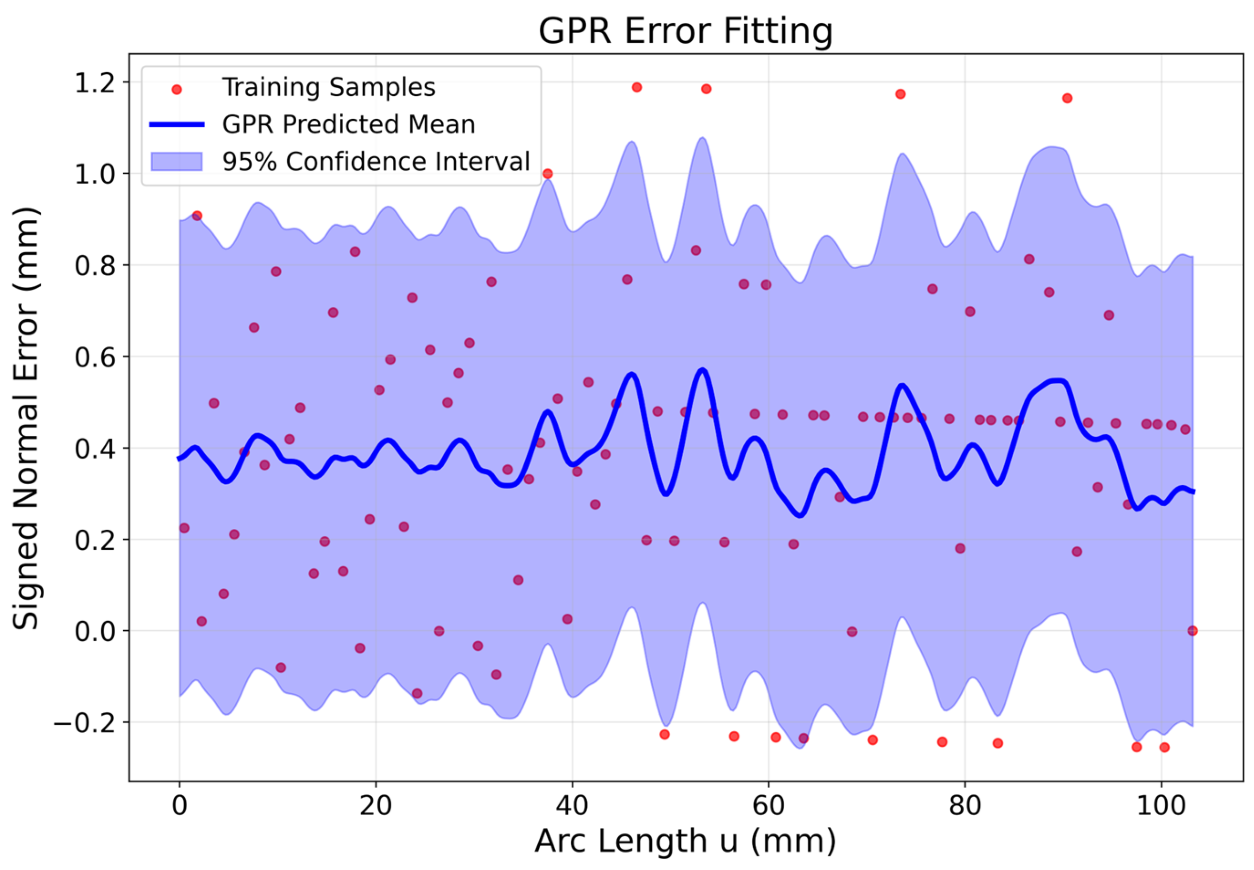
Rather than constructing separate models for each experimental dataset, the projection error samples from all three experiments were merged into a single training dataset and used to train a unified GPR error model. The original dataset contained 370 projection samples. After applying arc-length-based binning and averaging for data smoothing, 102 training samples were obtained for model fitting.

The model hyperparameters, including the signal variance, characteristic length scale, and noise level, were jointly optimized using the merged training dataset by maximizing the log marginal likelihood function.

The error function can then be modeled as a stochastic process with respect to the arc-length parameter $u$:

$$e\left(u\right)\sim \mathcal{G}\mathcal{P}(0,k(u,u^{\prime }\left)\right)$$

(21)

where $\mathcal{G}\mathcal{P}$ denotes the Gaussian process, and $k(u,u^{\prime })$ is the covariance function that characterizes the correlation of errors between different trajectory positions.

Considering that the roller trajectory error exhibits local continuity along the arc-length direction while potentially containing local fluctuations, the Matérn kernel is selected as the covariance function. The smoothness parameter $\mathsf{\nu }$ in the Matérn kernel controls the differentiability of the function. When $\nu =1.5$, the resulting function is once differentiable, ensuring global continuity while preserving local variations. Since the roller trajectory error is generally continuous but may exhibit local irregularities due to machining disturbances and measurement noise, an overly smooth kernel may lead to excessive smoothing of error details. Therefore, the Matérn kernel with $\nu =1.5$ is adopted to achieve a balance between smoothness and local fitting capability. Its expression is given by:

$$k(u,u^{\prime })={\sigma }^2\left(1+{\displaystyle \frac{\sqrt{3}r}{l}}\right)\mathit{exp}\left(-{\displaystyle \frac{\sqrt{3}r}{l}}\right)$$

(22)

where

$$r=|u-u^{\prime }|$$

(23)

Here, ${\sigma }^2$ is the signal variance representing the overall magnitude of the error, and $l$ is the characteristic length scale controlling the smoothness of the error variation along the arc length. A larger $l$ leads to smoother predictions, while a smaller $l$ enables the model to capture more localized variations.

To further account for unavoidable noise in the measured data, a white noise term is added to the kernel function, resulting in the total covariance function:

$$k_{total}(u,u^{\prime })=k_{matern}(u,u^{\prime })+{\sigma }_n^2\delta (u,u^{\prime })$$

(24)

where ${\sigma }_n^2$ is the noise variance, and $\delta (u,u^{\prime })$ is the Kronecker delta function, indicating that measurement noise only affects individual sample points.

In the model implementation, a composite kernel consisting of a constant kernel, a Matérn kernel, and a white noise kernel is employed. The constant kernel adjusts the overall signal magnitude, the Matérn kernel captures the local smooth characteristics of the trajectory error, and the white noise kernel suppresses the influence of measurement noise on the fitting results. The hyperparameters of the model, including the length scale, noise level, and signal variance, are automatically optimized by maximizing the log marginal likelihood, defined as:

$$\mathit{log}p(e|u)=-{\displaystyle \frac{1}{2}}{e}^T{K}^{-1}e-{\displaystyle \frac{1}{2}}\mathit{log}|K|-{\displaystyle \frac{n}{2}}log2\pi$$

(25)

where $e$ is the training error vector, $K$ is the covariance matrix constructed from the kernel function, and $n$ is the number of training samples. By optimizing this objective function, the optimal combination of hyperparameters can be obtained, thereby improving the fitting accuracy of the model. To mitigate the effects of step-like fluctuations and repeated sampling points in the measured trajectory on the Gaussian Process Regression (GPR) model, the training data were preprocessed using an arc-length-based binning and averaging strategy. Specifically, the trajectory was divided into intervals with a bin width of 1.0 mm, and the error values within each interval were averaged to obtain a set of smoothed training samples for subsequent model fitting.

After training, the GPR model can provide the predicted mean $e\left(u^{*}\right)$ and standard deviation $\sigma \left(u^{*}\right)$ of the error at any given arc-length position $u^{*}$. The predicted mean represents the magnitude of the systematic error at that position, while the standard deviation reflects the uncertainty of the model prediction, as shown in Figure 22. Based on these results, a trajectory compensation model can be further constructed to achieve adaptive correction of the simulated trajectory.

Figure 22. Error Fitting Based on Gaussian Process Regression.

4.1.3. Trajectory Compensation Model

Based on the error prediction results obtained from the Gaussian Process Regression (GPR) model, the simulated trajectory is corrected along the normal direction to achieve precise compensation of the roller motion trajectory. Let the simulated trajectory be represented as a parametric curve $C\left(u\right)$. The compensated trajectory can then be expressed as:

$$C_{comp}\left(u\right)=C\left(u\right)-\widehat{e}\left(u\right)\hspace{0.17em}n\left(u\right)$$

(26)

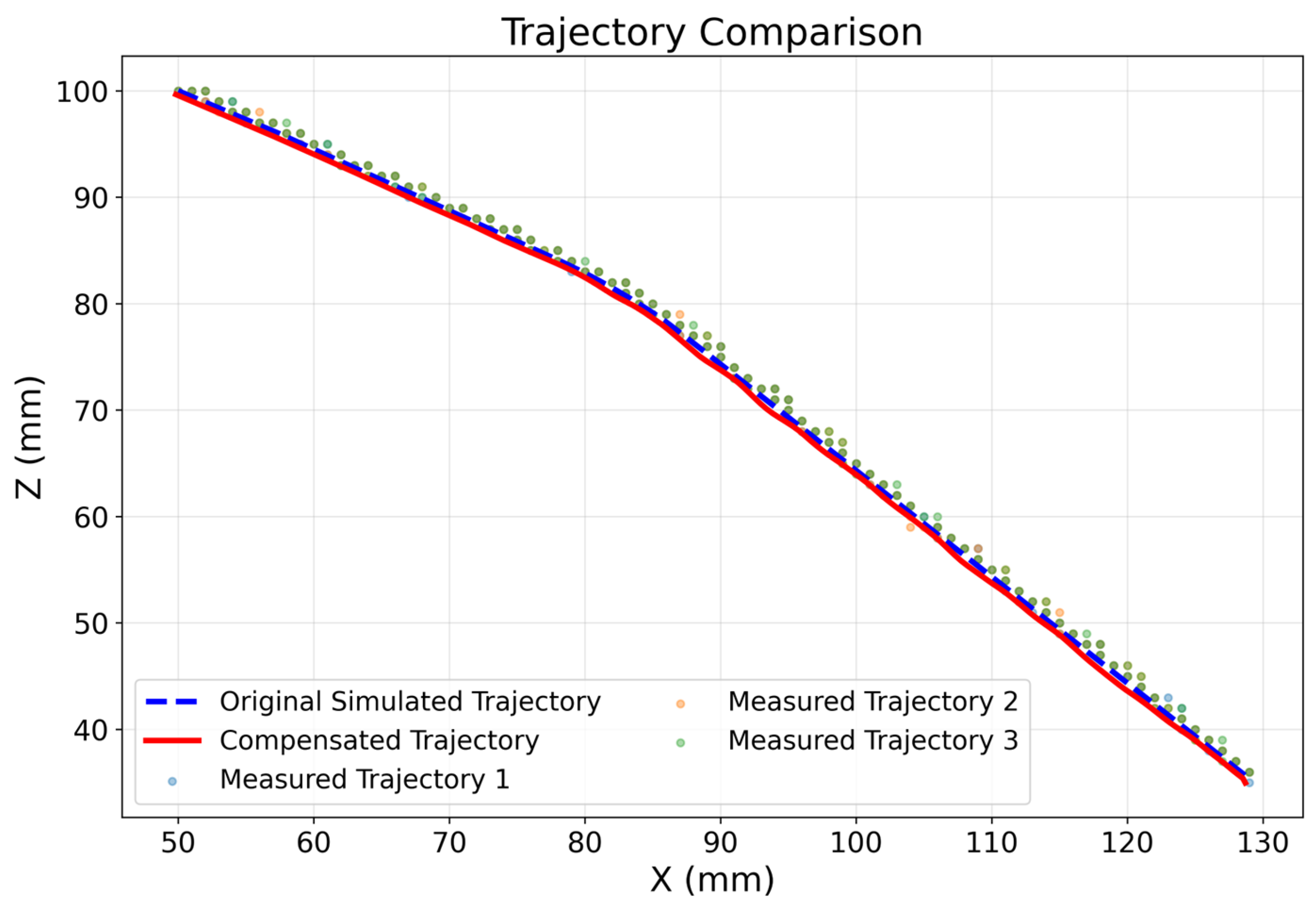
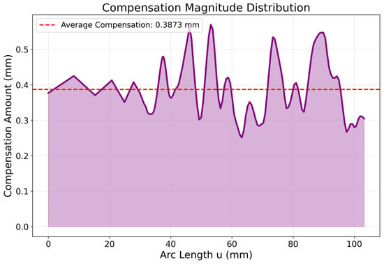
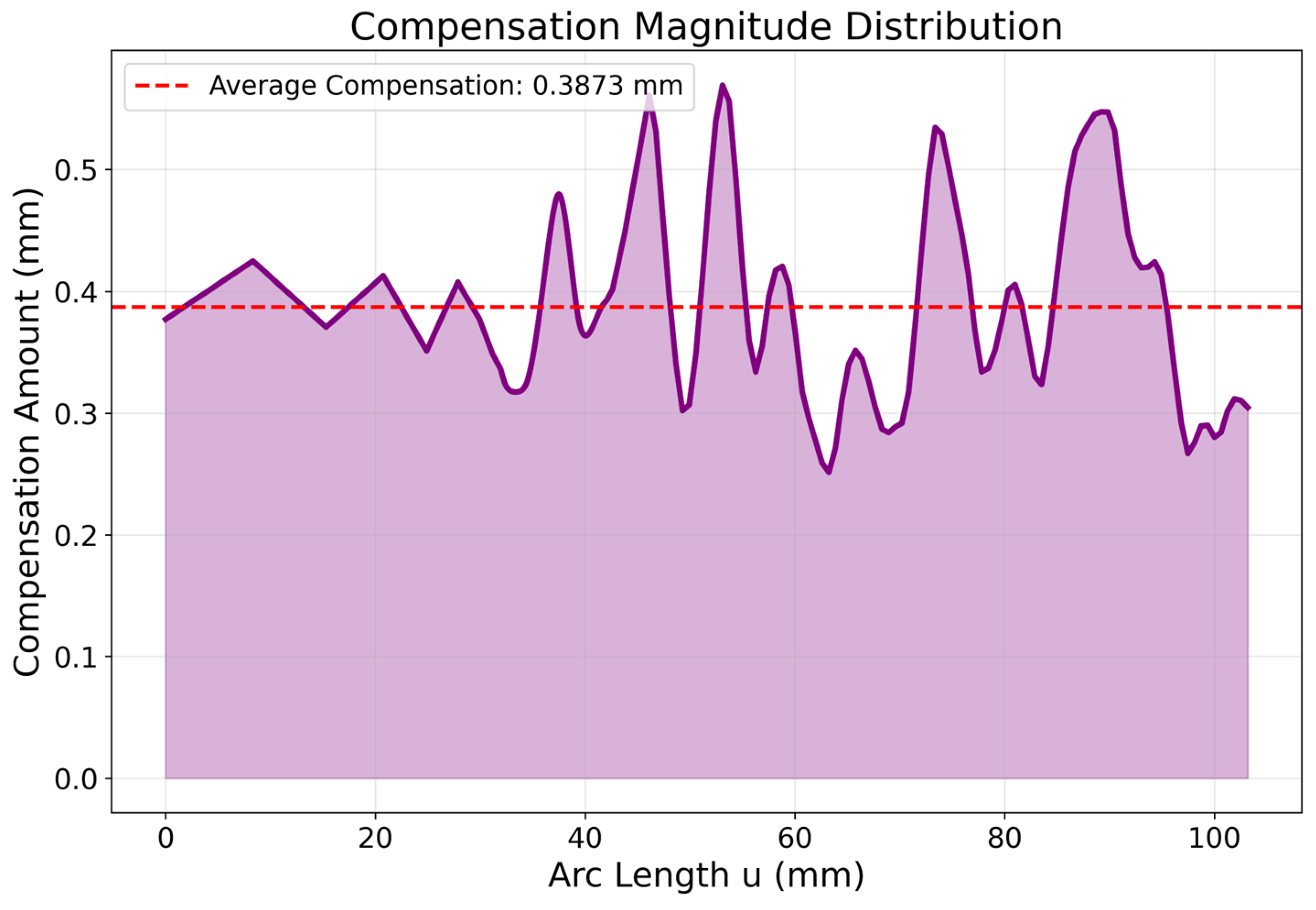
where $\widehat{\mathrm{e}}\left(\mathrm{u}\right)$ is the predicted mean error at arc-length parameter $u$ obtained from the GPR model, and $n\left(u\right)$ is the unit normal vector of the trajectory at the corresponding position. The coordinates of the compensated trajectory are listed in Table 10. The overall comparison of the trajectories after compensation is shown in Figure 23, and the distribution of the trajectory compensation values is illustrated in Figure 24.

Table 10. The coordinates of the compensated trajectory (see Supplementary Materials, Table S6 for details).

Number of Data Points (n)	X-Coordinate of the Compensated Trajectory	Z-Coordinate of the Compensated Trajectory
1	49.8316	99.6625
2	57.1197	95.6806
3	63.1843	92.2391
4	67.8837	89.4823
5	71.4940	87.4660
6	74.0469	85.9265
7	75.8298	84.9338
8	76.9681	84.307
9	77.5985	83.9603
$⋮$	$⋮$	$⋮$
184	128.6955	34.9855

Figure 23. Overall Comparison of Trajectories Before and After Compensation.

Figure 24. Distribution of Trajectory Compensation Values.

The physical interpretation of this compensation method is that the predicted systematic error is corrected in the opposite direction along the trajectory normal, thereby bringing the compensated trajectory closer to the actual machining trajectory. Compared with direct correction of coordinate components, this method fully accounts for the local geometric characteristics of the trajectory and effectively avoids error amplification in the tangential direction.

4.2. Experimental Validation

On this basis, the compensated trajectory was re-executed on the machine tool, and the actual machine trajectory was acquired. A comparative error analysis was then conducted between the compensated simulated trajectory and the measured trajectory to validate the effectiveness of the proposed compensation method. The coordinates of the compensated trajectory are presented in Table 11.

Table 11. Measured Trajectory Coordinates After Compensation (see Supplementary Materials, Table S7 for details).

Number of Data Points (n)	Measured X Coordinates	Measured Z Coordinates
1	50	100
2	51	99
3	51	99
4	52	98
5	53	98
6	54	98
7	54	97
8	55	97
9	56	96
$⋮$	$⋮$	$⋮$
118	129	35

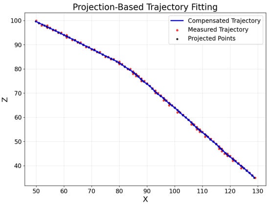
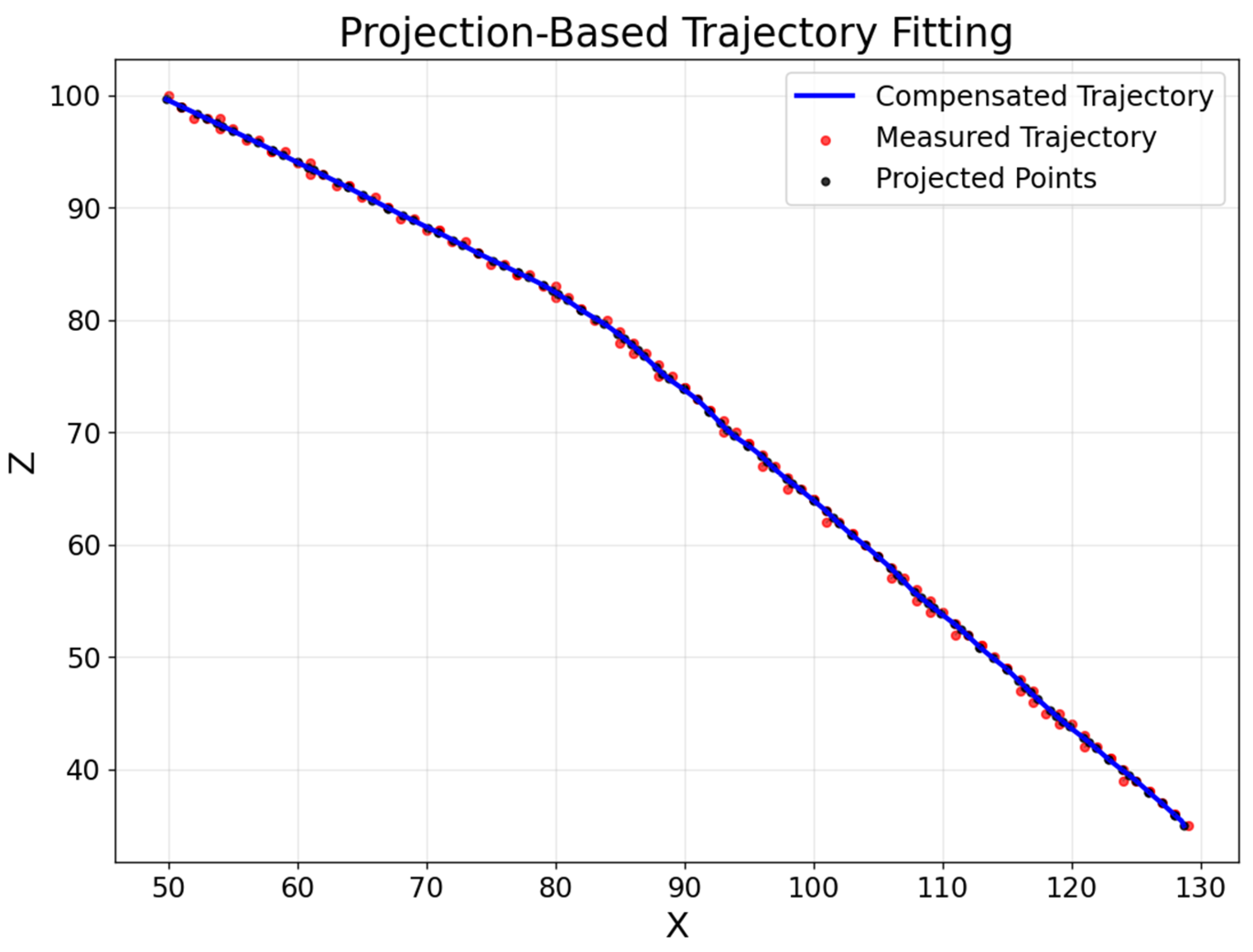
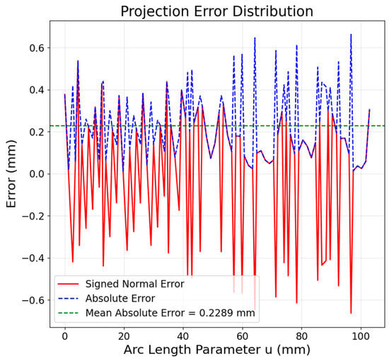
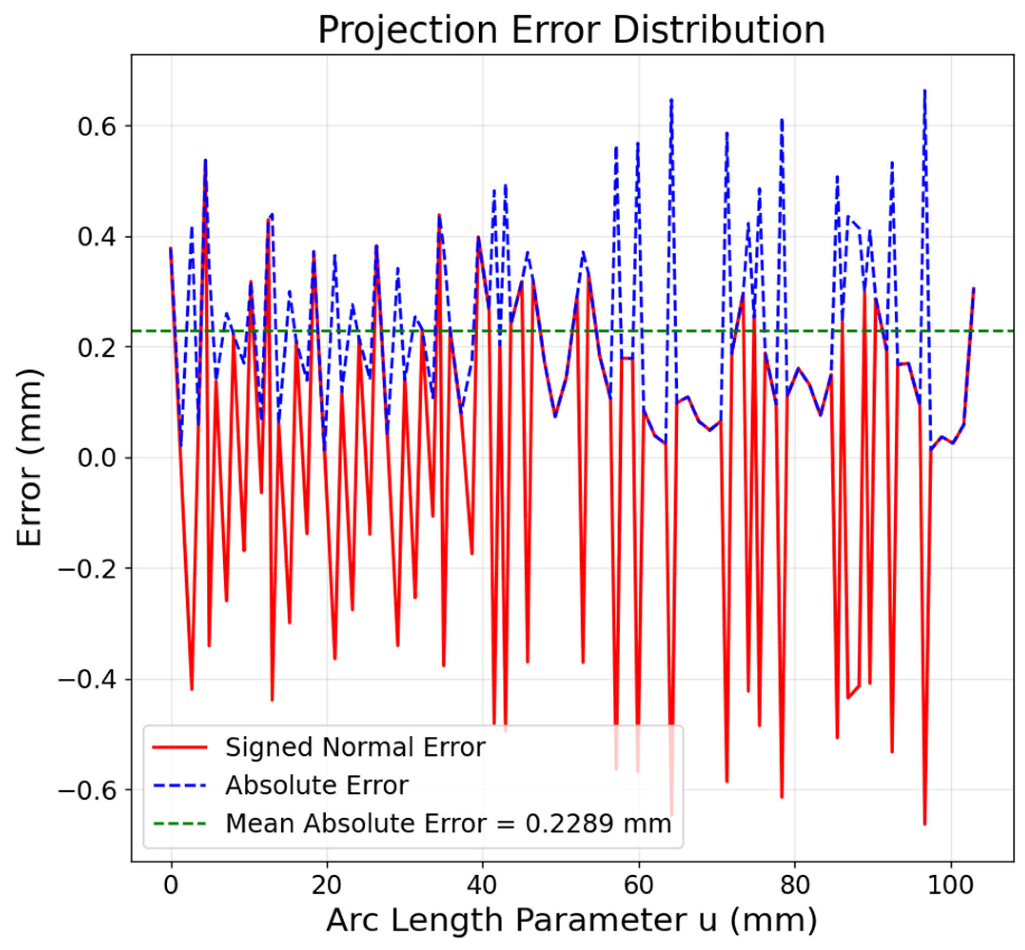
The trajectory fitting results are shown in Figure 25. The experimental results indicate that the average deviation between the compensated actual trajectory and the compensated simulated trajectory is 0.229 mm. Compared with the average deviation of 0.503 mm before compensation, the error is reduced by 54.47%. The error distribution is shown in Figure 26.

Figure 25. Trajectory Fitting Results.

Figure 26. Distribution of Projection Errors.

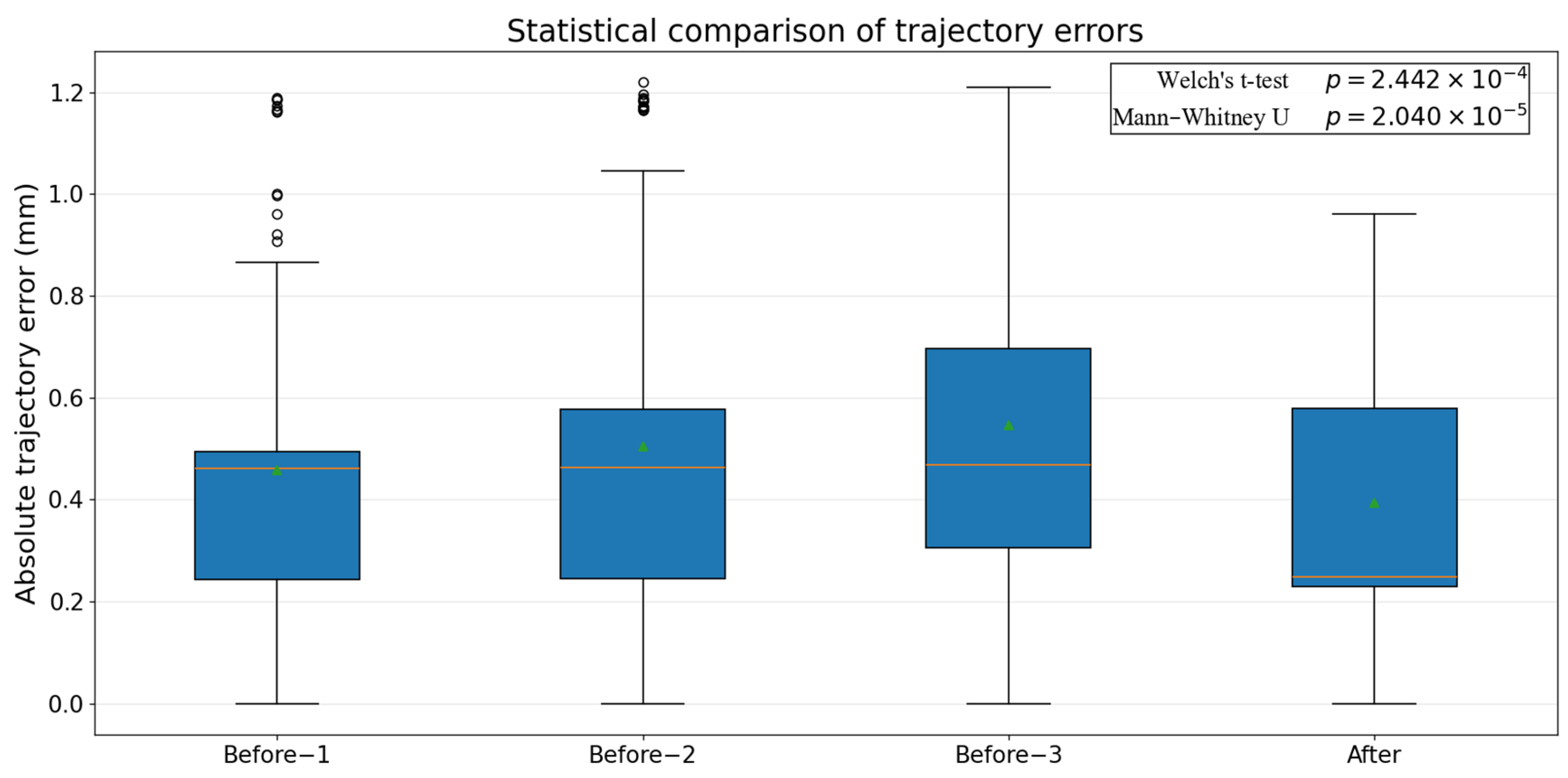
To evaluate the effectiveness of the proposed trajectory error compensation method, a statistical analysis was performed on the trajectory errors before and after compensation. First, the three uncompensated measured trajectories and the compensated measured trajectory were projected onto the original finite element (FE) simulated trajectory, and the absolute projection error between each measured point and the reference trajectory was calculated. The absolute projection error was adopted as the trajectory accuracy metric to eliminate the influence of error direction on the statistical evaluation.

The uncompensated error dataset consisted of all projection errors obtained from the three uncompensated experiments, whereas the compensated error dataset consisted of all projection errors obtained from the compensated experiment. Descriptive statistics, including the mean, median, standard deviation, and root mean square error (RMSE), were calculated for both datasets. The reduction in the mean error was used to quantify the effectiveness of the compensation method.

Considering that the variances of the two datasets might not be equal, Welch’s t-test was employed to compare the mean errors before and after compensation. In addition, a non-parametric Mann–Whitney U test was conducted to verify the robustness of the results against potential deviations from normality. For both tests, the alternative hypothesis was defined as the compensated trajectory errors being significantly smaller than the uncompensated trajectory errors. The significance level was set at α = 0.05. A result was considered statistically significant when the p-value was less than 0.05.

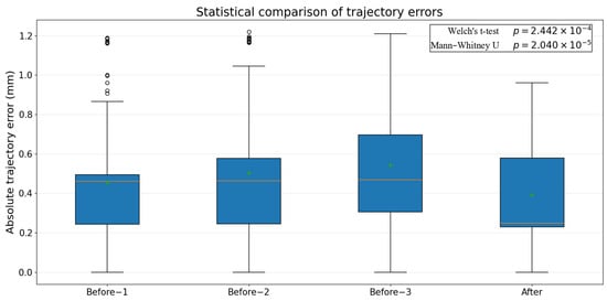
The statistical results demonstrated a significant reduction in trajectory error after compensation. As shown in Figure 27, the p-values obtained from Welch’s t-test and the Mann–Whitney U test were 2.442 × 10⁻⁴ and 2.040 × 10⁻⁵, respectively, both of which were substantially lower than the significance threshold of 0.05. These results indicate that the observed improvement in trajectory accuracy was unlikely to be caused by random variation and can therefore be attributed to the proposed compensation method.

Figure 27. Statistical Significance Analysis of the Compensation Effect.

These results demonstrate that the proposed trajectory error compensation method based on the projection method and Gaussian Process Regression significantly improves trajectory consistency and effectively reduces the deviation between the actual machining trajectory and the simulated trajectory. Consequently, the accuracy and reliability of simulation-based guidance for the spinning process are substantially enhanced.

5. Conclusions

This study focuses on the application of roller trajectories for double-conical spinning parts from finite element simulation to actual machine tool execution. A systematic investigation is conducted to address key issues, including the difficulty of directly applying simulated trajectories to machine control and the deviation between simulated and actual trajectories. The main contributions and conclusions are summarized as follows:

(1)

Based on finite element simulation using ABAQUS, a forming model for double-conical spinning parts is established. To overcome the limitation that analytical rigid rollers cannot directly output motion trajectories, an indirect trajectory extraction method is proposed by introducing a discrete shell combined with geometric relationships. This approach enables accurate extraction of the roller center trajectory and transforms the continuous simulation process into a discrete coordinate sequence. Furthermore, to address the discrepancy between the simulation and machine tool coordinate systems, a coordinate transformation method is developed. Through coordinate origin alignment, spatial rotation, and translation operations, the simulated trajectory is successfully converted into a machine-executable trajectory.

(2)

A roller trajectory acquisition method based on displacement sensors is developed to obtain actual motion trajectory data from the spinning machine. By integrating curve fitting and projection methods, the correspondence between the actual trajectory and the simulated trajectory is established, and quantitative error analysis is performed.

(3)

To address the systematic deviation between simulated and actual execution trajectories, a trajectory error compensation method based on the projection method and Gaussian Process Regression (GPR) is proposed. The trajectory error is modeled as a scalar quantity along the curve normal direction, and the simulated trajectory is corrected accordingly based on the predicted error. This enables adaptive optimization of the trajectory. Experimental results demonstrate that the average trajectory error is reduced from 0.503 mm to 0.229 mm after compensation, significantly improving trajectory consistency and machining accuracy.

The present study primarily focuses on trajectory errors under single-roller spinning conditions, with emphasis on static trajectory deviations. Dynamic errors caused by machine tool dynamics, vibration, and control response during the spinning process are not considered. In addition, the error modeling is based on a limited set of experimental data, and its generalization capability under multiple operating conditions and complex machining scenarios requires further validation. Future work will incorporate dynamic error modeling methods and expand the experimental dataset to further enhance the applicability and robustness of the proposed trajectory compensation method in practical engineering applications.

References

- Music, O.; Allwood, J.M.; Kawai, K. A review of the mechanics of metal spinning. J. Mater. Process. Technol. 2010, 210, 3–23. [Google Scholar] [CrossRef] [Scilit]
- Wong, C.C.; Dean, T.A.; Lin, J. A review of spinning, shear forming and flow forming processes. Int. J. Mach. Tools Manuf. 2003, 43, 1419–1435. [Google Scholar] [CrossRef] [Scilit]
- Li, Y.; Wang, J.; Lu, G.-D.; Pan, G.-J. A numerical study of the effects of roller paths on dimensional precision in die-less spinning of sheet metal. J. Zhejiang Univ. Sci. A 2014, 15, 432–446. [Google Scholar] [CrossRef] [Scilit]
- Jia, Z.; Han, Z.R.; Liu, B.M.; Fan, Z.J. Numerical simulation and experimental study on the non-axisymmetric spinning of conical parts. Int. J. Adv. Manuf. Technol. 2017, 89, 2637–2648. [Google Scholar]
- Wang, L.; Long, H. A study of effects of roller path on spinning process by finite element simulation. J. Mater. Process. Technol. 2011, 211, 1037–1047. [Google Scholar]
- Majewski, M.; Gądek, T.; Klimek, L.; Nowacki, Ł. Comparison of spinning trajectory designing methods for products with non-circular cross-section. Manuf. Technol. 2022, 22, 503–510. [Google Scholar]
- Hayama, M.; Kudo, H.; Shinokura, T. Study of the pass schedule in conventional simple spinning. Bull. JSME 1970, 13, 1358–1365. [Google Scholar] [CrossRef] [Scilit]
- Ma, Z.P.; Sun, C.G. The effects of roller paths on the forming quality of conventional spinning process. Forg. Stamp. Technol. 1999, 1, 21–24. [Google Scholar]
- Liu, J.H. Multi-Passes Conventional Spinning Deforming Mechanism and Roller Paths Effects Research. Ph.D. Thesis, Northwestern Polytechnical University, Xi’an, China, 2003. [Google Scholar]
- Xia, Q.X.; Chen, S.X.; Cao, G.S.; Zhang, C.L.; Sun, Y. Conventional spinning of cone parts with involute model template. Forg. Stamp. Technol. 1993, 18, 22–24,26. [Google Scholar]
- Liu, X.J.; Zhang, Y.H. How to select the moving passes of the spinning roller. J. Plast. Eng. 1997, 4, 84–90. [Google Scholar]
- Chen, J.; Wan, M.; Li, W.D.; Xu, C.X.; Xu, X.D.; Huang, Z.B. Design of the involute trace of multi-pass conventional spinning and application in numerical simulation. J. Plast. Eng. 2009, 15, 53–57. [Google Scholar]
- Liu, F.Y.; Wang, A.L. The application of B spline curve in spinning manufacture process. Forg. Stamp. Technol. 1994, 2, 36–40. [Google Scholar]
- Liu, J.H.; Yang, H.; Li, Y.Q. A study of the stress and strain distributions of first-pass conventional spinning under different roller-traces. J. Mater. Process. Technol. 2002, 129, 326–329. [Google Scholar]
- Wang, L.; Long, H. A study of effects of roller path profiles on tool forces and part wall thickness variation in conventional metal spinning. J. Mater. Process. Technol. 2011, 211, 2140–2151. [Google Scholar] [CrossRef] [Scilit]
- Wei, Z.C.; Li, W.D.; Wan, M.; Xu, C.X.; Huang, Z.B.; Liu, J. Influence of roller-trace on multi-pass conventional spinning process. J. Plast. Eng. 2010, 17, 108–112. [Google Scholar]
- Zhan, M.; Li, H.; Yang, H.; Chen, G. Wall thickness variation during multi-pass spinning of large complicated shell. J. Plast. Eng. 2008, 15, 115–121. [Google Scholar]
- Wang, L.; Long, H. Roller path design by tool compensation in multi-pass conventional spinning. Mater. Des. 2013, 46, 645–653. [Google Scholar] [CrossRef] [Scilit]
- Wang, Q.; Wang, L.; Jiang, Z.; Gong, S. Algorithm for the generation of mandrel protection curve and trajectory scheme for spinning machine. Int. J. Adv. Manuf. Technol. 2013, 68, 217–226. [Google Scholar] [CrossRef] [Scilit]
- Gondo, S.; Arai, H. Roller path solver system for multi-objective task-priority control of multipass conventional spinning. Mech. Eng. J. 2023, 10, 22-00253. [Google Scholar]
- Gao, P.; Yan, X.; Wang, Y.; Li, H.; Zhan, M.; Ma, F.; Fu, M. An online intelligent method for roller path design in conventional spinning. J. Intell. Manuf. 2023, 34, 3429–3444. [Google Scholar]
- Liu, Y.; Chen, M.; Sun, Y. Global toolpath modulation-based contour error pre-compensation for multi-axis CNC machining. Int. J. Adv. Manuf. Technol. 2023, 125, 3171–3189. [Google Scholar] [CrossRef] [Scilit]
- He, W.; Zhang, L.; Hu, Y.; Zhou, Z.; Qiao, Y.; Yu, D. A hybrid-model-based CNC machining trajectory error prediction and compensation method. Electronics 2024, 13, 1143. [Google Scholar] [CrossRef] [Scilit]
- Wei, X.; Ye, H.; Miao, E.; Pan, Q. Thermal error modeling and compensation based on Gaussian process regression for CNC machine tools. Precis. Eng. 2022, 77, 65–76. [Google Scholar] [CrossRef] [Scilit]
- Wan, M.; Zhang, W. Calibration and compensation of machine tool volumetric error using Gaussian process regression. Int. J. Mach. Tools Manuf. 2018, 128, 81–93. [Google Scholar]
- Schwenke, H.; Knapp, W.; Haitjema, H.; Weckenmann, A.; Schmitt, R.; Delbressine, F. Geometric error measurement and compensation of machines—An update. CIRP Ann. 2008, 57, 660–675. [Google Scholar] [CrossRef] [Scilit]
- Geng, Z.; Tong, Z.; Jiang, X. Review of geometric error measurement and compensation techniques of ultra-precision machine tools. Light Adv. Manuf. 2021, 2, 211–227. [Google Scholar] [CrossRef] [Scilit]
Disclaimer/Publisher’s Note: The statements, opinions and data contained in all publications are solely those of the individual author(s) and contributor(s) and not of MDPI and/or the editor(s). MDPI and/or the editor(s) disclaim responsibility for any injury to people or property resulting from any ideas, methods, instructions or products referred to in the content. |
© 2026 by the authors. Licensee MDPI, Basel, Switzerland. This article is an open access article distributed under the terms and conditions of the Creative Commons Attribution (CC BY) license.