


Abstract
Accurate vehicle state estimation is a critical prerequisite for electric vehicle motion control, yet its performance is highly sensitive to deviations in inertial parameters. Variations in vehicle mass and moment of inertia caused by changing loads can lead to model mismatch, thereby degrading the accuracy and robustness of state estimation. To this end, this paper proposes a hierarchical collaborative estimation framework that integrates the Maximum Correntropy Adaptive Unscented Kalman Filter (MCAUKF) with a Physics-Informed Neural Network (PINN) for inertial parameter identification and key state estimation in electric vehicles. The upper layer employs MCAUKF for robust online identification of unknown inertial parameters, such as vehicle mass and moment of inertia. The lower layer develops a PINN-based state estimator that incorporates physical constraints by embedding the coupled dynamic residuals of longitudinal, lateral, and roll motions into the supervised learning process, thereby enabling high-precision real-time estimation of key dynamic states, including yaw angle, longitudinal velocity, and roll angle. Simulation results demonstrate that the proposed method can effectively achieve coordinated estimation of inertial parameters and key states under varying load conditions and complex maneuvering scenarios, significantly improving overall estimation accuracy and robustness.
1. Introduction
As a vehicle that deeply integrates new energy and intelligent connected technologies, the electric vehicle has become a key enabler for promoting the green, low-carbon, and intelligent transformation of transportation systems [1]. Among them, distributed drive electric vehicles allow each wheel to be directly driven or braked by an independent motor, offering advantages such as fast torque response, high control flexibility, and strong actuator redundancy. These characteristics provide a more flexible platform for torque-vectoring control, energy-oriented torque allocation, and vehicle stability control [2,3]. However, the effective implementation of these control functions relies heavily on accurate perception of vehicle dynamic states and inertial parameters [4,5]. Key dynamic states, such as the vehicle sideslip angle, longitudinal velocity, and roll angle, characterize the transient response and operational stability of the vehicle [6]. Inertial parameters, including vehicle mass and moment of inertia, determine the dynamic characteristics and model accuracy of the vehicle, and thus serve as important references for controller design and implementation. However, due to limitations in sensor cost and measurement accuracy, these states are often difficult to obtain directly. In addition, load variations can cause the vehicle’s inertial parameters to deviate from their nominal values, resulting in model mismatch and further degrading the accuracy and robustness of state estimation and control decisions [7]. Therefore, developing methods for the coordinated estimation of high-precision inertial parameters and key states holds significant theoretical and engineering value [8].
Existing vehicle state estimation methods primarily include model-based methods [9], learning-based methods [10], and methods that integrate modeling and learning [11]. Model-based methods achieve online estimation of unobservable states by establishing state space models of vehicle dynamics and measurement equations, combined with observers or recursive filtering algorithms [12]. These methods have clear physical meaning, are highly interpretable, and exhibit low data dependency; therefore, they are widely used in vehicle state estimation [13]. Among these, Kalman filtering and its variants are the most representative [14,15]. For example, Ren et al. [16] employed UKF to achieve real-time estimation of vehicle longitudinal and lateral velocities, yaw rate, and tire-related states; Wang et al. [17] proposed AUKF, which improved filtering stability by dynamically adjusting noise statistics. To address the low accuracy of vehicle state and parameter estimation under non-Gaussian conditions, Zhang et al. [18] proposed a joint estimation algorithm based on the Maximum Correntropy Adaptive Unscented Kalman Filter (MCAUKF), enabling high precision estimation of vehicle motion states and key inertial parameters. Although model-based methods possess good online recursive capabilities, their performance is highly dependent on model accuracy. In particular, when load changes cause inertial parameters to deviate from their nominal values, model mismatch and unmodeled dynamics will jointly reduce estimation accuracy and robustness [19].
To overcome the limitations imposed by model dependency, data-driven methods have garnered significant attention in recent years [20]. With the advancement of deep learning, learning-based methods can utilize neural networks to uncover complex nonlinear mappings between sensor inputs and target states, demonstrating strong advantages in handling strongly coupled and unknown nonlinear dynamics [21,22]. For example, Xing et al. [23] utilized deep recurrent neural networks with LSTM units to estimate the dynamic brake pressure of electric vehicles; Kong et al. [24] proposed an LSTM-based method for estimating lateral velocity; and Zhang et al. [25] proposed a deep learning-based method for the direct estimation of tire volume. Although data-driven methods offer advantages in feature extraction and nonlinear mapping, their lack of explicit physical constraints limits their generalization capability and interpretability under complex and unknown operating conditions. As a result, they may fail to meet the high-accuracy and high-reliability requirements of safety-critical applications [26].
Consequently, methods that integrate models and learning have gradually emerged as a research focus. Their core lies in combining the interpretability of mechanistic models with the adaptive representational capabilities of data-driven methods to improve the accuracy and robustness of vehicle state estimation [27]. Li et al. [28] proposed a hybrid physical data-driven observer that employs ridge regression and an LSTM network with a two-stage attention mechanism to estimate vehicle dynamic states. To address the limited ability of the UKF to suppress sensor bias, Tan et al. [29] proposed a vehicle state estimation method that integrates a Physics-Informed Neural Network (PINN) with UKF-M, achieving high precision estimation of the vehicle’s 3D attitude, velocity, and position; PINN embeds vehicle dynamics equations directly into the network’s loss function, enabling the model to satisfy physical constraints while approximating the data. Consequently, they demonstrate superior accuracy, robustness, and interpretability under conditions of strong nonlinearity, strong coupling, and unknown operating conditions [30]. However, most existing model-learning fusion methods mainly focus on vehicle dynamic state estimation, with limited consideration of load-induced inertial parameter deviations and their coupling relationships with key dynamic states.
Many existing vehicle state estimation methods assume that inertial parameters, such as vehicle mass and moment of inertia, are known constants [31]. However, during real-world driving, variations in the number of passengers and cargo load can lead to significant changes in vehicle mass and moment of inertia [32]. For example, the mass and center-of-gravity position may differ considerably between unloaded and fully loaded conditions. Such variations in inertial parameters directly affect tire vertical load distribution, yaw response, roll motion, and longitudinal–lateral coupled dynamics [33]. If fixed nominal parameters are still used for state estimation, model mismatch may occur, thereby degrading the estimation accuracy and robustness of key states such as sideslip angle, longitudinal velocity, and roll angle [34]. Therefore, it is important to account for inertial parameter variations during vehicle state estimation.
To address the coupled estimation of states and parameters, various joint estimation, dual estimation, and staged estimation methods have been proposed. For example, an H∞-EKF-based method has been used for center-of-gravity position estimation [35]; DEKF-based methods have been applied to identify parameters such as vehicle mass, center-of-gravity position, and moment of inertia [36]; and some studies have augmented the state vector with vehicle mass, center-of-gravity height, and yaw moment of inertia, using recursive filtering algorithms such as UKF to achieve joint state and parameter estimation [37]. These studies indicate that inertial parameter identification can effectively improve vehicle state estimation performance, particularly under load-varying conditions and complex maneuvering scenarios [38].
However, existing methods still have several limitations. First, joint estimation methods based on augmented state vectors significantly increase the system dimensionality and nonlinear coupling, leading to more complex filter design and higher online computational burden. Second, although dual-filter and staged estimation methods can alleviate the coupling between states and parameters to some extent, their performance still strongly depends on the accuracy of the vehicle dynamics model, tire model, and noise statistical characteristics. Third, inertial parameter identification and vehicle dynamic state estimation are inherently different tasks: the former aims to accurately identify unknown parameters such as vehicle mass and moment of inertia, whereas the latter focuses on real-time tracking of dynamic states. If a single estimator or a unified data-driven network is used to handle both tasks simultaneously, conflicts may arise between parameter identification stability and state tracking accuracy. In addition, multitask coupling may introduce training interference and further degrade the robustness and generalization capability of the model.
Therefore, a hierarchical collaborative estimation framework integrating Maximum Correntropy Adaptive Unscented Kalman Filtering and a Physics-Informed Neural Network (MCAUKF-PINN) is proposed. The proposed framework decouples the joint estimation problem into two hierarchical layers according to the distinct roles of inertial parameter identification and dynamic state estimation. In the upper layer, MCAUKF is employed to achieve robust online identification of unknown inertial parameters, including vehicle mass and moment of inertia. In the lower layer, a physics-constrained PINN estimator is developed to accurately estimate key dynamic states, including sideslip angle, longitudinal velocity, and roll angle. Furthermore, the identified inertial parameters are embedded into the coupled longitudinal lateral roll dynamic residuals as physical priors, thereby enabling coordinated estimation of inertial parameters and key dynamic states.
The main contributions of this paper are summarized as follows:
- A hierarchical collaborative estimation framework is developed for unknown inertial parameters and key vehicle states. By hierarchically decoupling inertial parameter identification from dynamic state estimation according to their distinct task characteristics, the proposed framework enables collaborative and accurate estimation of both inertial parameters and key states.
- An inertial parameter estimator based on MCAUKF is developed. By incorporating a maximum correntropy-based adaptive weighting mechanism and a noise statistics adjustment strategy into the UKF recursive update, the proposed estimator improves the accuracy and robustness of online identification of vehicle mass and moment of inertia under uncertain noise conditions.
- Design a PINN state estimator that integrates physical constraints. By combining the results of the upper-layer inertial parameter estimation, the residual constraints derived from the coupled dynamics of longitudinal, lateral, and roll motions are embedded into the supervised learning process, enabling high-precision real-time estimation of the center of mass slip angle, longitudinal velocity, and roll angle.
The remainder of this paper is organized as follows. Section 2 presents the vehicle dynamics model and problem formulation. Section 3 introduces the hierarchical estimation framework, the upper-layer inertial parameter identification method, and the design and training strategy of the lower-layer PINN state estimator. Section 4 provides simulation results and comparative analysis. Finally, Section 5 concludes the paper and discusses future work.
2. Vehicle Dynamics Model
2.1. 4-DOF Vehicle Dynamics Model
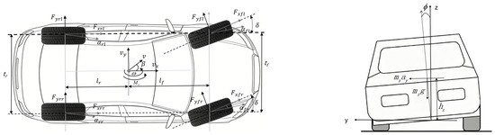
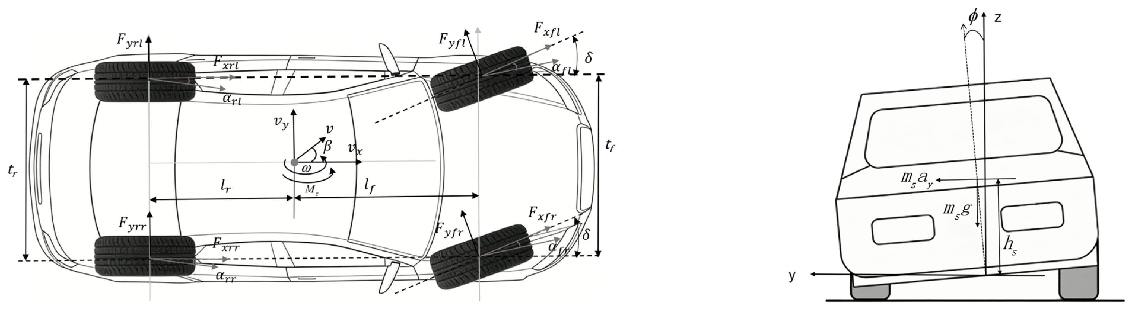
A four-degree-of-freedom (4-DOF) vehicle dynamics model, including longitudinal, lateral, yaw, and roll motions, together with a tire model, is established in this study, as illustrated in Figure 1. The proposed model can effectively capture the dominant dynamic behaviors of the vehicle under complex operating conditions and provides a unified physical basis for subsequent estimation of inertial parameters and key states. To simplify the modeling process while preserving the main dynamic characteristics, the following assumptions are made: (1) the vehicle is laterally symmetric, and its center of mass lies on the longitudinal symmetry plane of the vehicle coordinate system; (2) suspension kinematic nonlinearities and the pitch degree of freedom are neglected, and only longitudinal, lateral, yaw, and roll motions are considered; (3) the front wheel steering angle is accurately provided by the steering system, and the left and right front wheels have identical steering angles; and (4) the effects of aerodynamic drag and tire rolling resistance on vehicle dynamics are neglected.
Figure 1.
Schematic diagram of the 4-DOF vehicle dynamics model.
Table 1 lists the baseline vehicle parameters under unloaded conditions. For the load varying simulation scenarios, the vehicle mass and moment of inertia are adjusted according to the prescribed load conditions in CarSim. The equations of the 4-DOF vehicle dynamics model are given as follows:
where and denote the longitudinal and lateral velocities at the vehicle center of mass, respectively. is the yaw rate, and is the roll angle. and represent the total vehicle mass and the sprung mass, respectively, and is the equivalent height from the sprung mass center of gravity to the roll axis. and denote the yaw moment of inertia and roll moment of inertia, respectively. and are the distances from the center of mass to the front and rear axles, respectively, while and are the front and rear track widths. denotes the front wheel steering angle. and represent the longitudinal and lateral tire forces, respectively, where denotes the front or rear axle, and denotes the left or right wheel. Specifically, , , , and correspond to the front-left, front-right, rear-left, and rear-right wheels, respectively. and denote the equivalent roll damping and roll stiffness of the suspension, respectively, and is the gravitational acceleration. and denote the longitudinal and lateral accelerations at the vehicle center of mass, respectively, and are defined as and .
Table 1.
Baseline vehicle dynamic model parameters.
2.2. Pacejka Tire Model
For distributed drive vehicles, the driving and braking torques of each wheel can be independently regulated, and the resulting wheel rotational dynamics directly influence the evolution of the tire slip ratio. The wheel rotational equilibrium can be expressed as follows:
where denotes the wheel end driving or braking torque, is the wheel rotational inertia, represents the wheel angular velocity, and is the tire rolling radius.
The general form of the Pacejka model can be written as
where denotes the variable to be calculated, namely the longitudinal force or lateral force, and represents either the slip angle or the slip ratio . The parameters , , , and are the stiffness factor, shape factor, peak factor, and curvature factor, respectively.
The slip ratio of each wheel is defined as
where is the effective rolling radius of the tire, and denotes the longitudinal velocity at the wheel center.
Under the small-angle assumption, the slip angles of the four wheels can be expressed as
where is the wheelbase, and is the height of the center of gravity.
3. Methodology
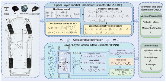
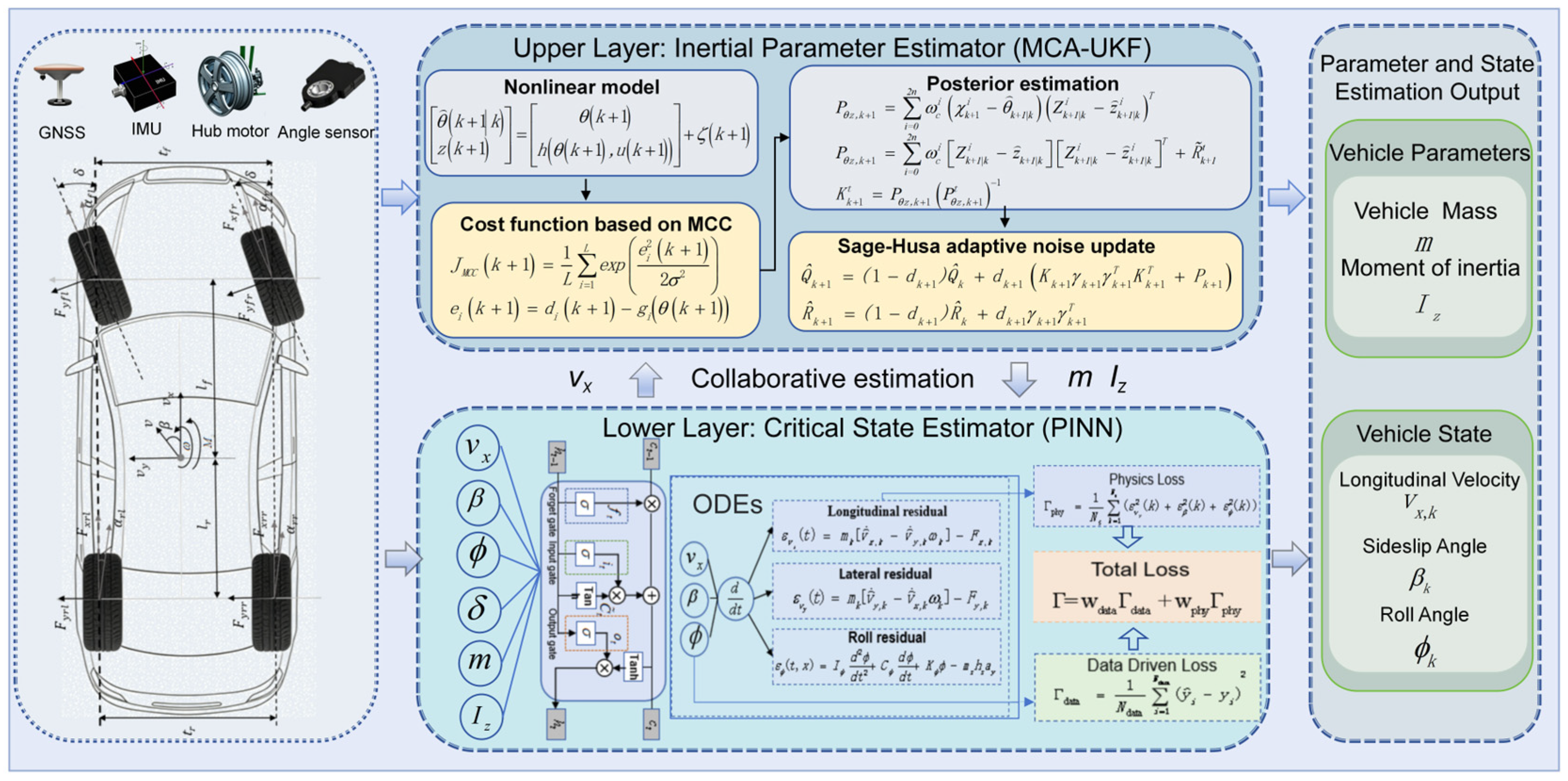
This paper proposes a hierarchical collaborative estimation framework that integrates MCAUKF and PINN to achieve synchronous online estimation of inertial parameters and key dynamic states for distributed drive electric vehicles. The overall architecture is shown in Figure 2. Considering the significant differences in time scales between inertial parameters and dynamic states, the upper layer constructs an inertial parameter estimator based on MCAUKF, utilizing a nonlinear state space model to perform recursive estimation of the vehicle mass and yaw moment of inertia . During the posterior update process, a cost function based on the maximum correlation entropy criterion is introduced, combined with the Sage Husa adaptive noise statistics update strategy, to perform online adjustment of the process noise and measurement noise covariance, thereby enhancing the estimation accuracy of the inertial parameters. The lower layer constructs a PINN-based key state estimator that uses historical measurement sequences and the time-varying inertial parameters output by the upper layer as inputs to perform high-precision estimation of the vehicle’s longitudinal velocity, slip angle, and roll angle. Furthermore, the physical residuals corresponding to the coupled longitudinal, lateral, and roll dynamic equations are introduced as constraint terms. Cooperative estimation is achieved through the bidirectional exchange of inertial parameters and state information between the upper and lower layers. This hierarchical cooperative strategy effectively avoids the issues of dimensionality explosion and strong coupling found in traditional unified dimension expansion joint estimation. While ensuring online feasibility, it significantly improves estimation accuracy and robustness under complex operating conditions.
Figure 2.
Co-estimation of vehicle state and control/inertial parameters using MCAUKF-PINN.
3.1. Estimation of Upper-Level Inertial Parameters Using MCAUKF
To address the shifts in inertial parameters such as vehicle mass and yaw moment of inertia caused by load changes and their adverse effects on control performance, this paper proposes an MCAUKF-based inertial parameter estimator. While retaining the UKF ability to perform recursive estimation for nonlinear systems, this method introduces the maximum relevant entropy criterion and models the higher order statistical characteristics of the error using a kernel function to enhance the algorithm’s robustness in unknown noise environments; simultaneously, by incorporating an adaptive noise covariance update mechanism, it further mitigates the impact of statistical uncertainty in noise on filtering accuracy, thereby achieving high precision online identification of unknown inertial parameters such as vehicle mass and yaw moment of inertia.
Define the system state variable as
where denotes the vehicle mass, and denotes the yaw moment of inertia.
The discrete-time state equation and measurement equation can be uniformly expressed as follows:
where is the input vector, and is the observation vector. The functions and denote the parameter, state transition function and measurement function, respectively. Moreover, and represent the process noise and measurement noise, with corresponding covariance matrices denoted by and , respectively.
During the time update stage, the MCAUKF follows the unscented transformation principle and constructs sigma points based on the state mean and covariance matrix :
where denotes the dimension of the parameter state, with . is the scaling factor, defined as
where controls the spread of the sigma points, and is an auxiliary scaling factor, which is typically set to .
By substituting the sigma points into the parameter state equation, the predicted sigma points are obtained.
The predicted mean and covariance are then computed as follows:
The weights are computed using the standard UKF formulation:
where is introduced to incorporate higher order information of the prior state distribution, .
Measurement update with the MCC. The predicted sigma points are mapped into the measurement space:
The following joint recursive form is constructed:
where denotes the joint error vector, and its covariance matrix can be expressed as:
where
By performing Cholesky decomposition on the joint covariance matrix, the standard residual model can be obtained:
The maximum correntropy cost function is defined as
where denotes the dimension of the vector , with , and is the kernel bandwidth parameter.
The residual component is defined as
where and denote the -th elements of and , respectively.
The optimization problem is solved using a fixed-point iteration method, and the update equation is given by
To realize adaptive weighting under the MCC, a diagonal weighting matrix is constructed as
The equivalent covariance matrix is defined as
where denotes the equivalent measurement noise covariance matrix weighted by the maximum correntropy criterion.
The predicted measurement mean, measurement covariance, and cross covariance are computed as follows:
The equivalent Kalman gain at the -th iteration is given by
When the convergence criterion is satisfied, the iteration is terminated, and the final result is taken as the posterior estimate of the inertial parameters, denoted by . The convergence criterion is given by
The converged result is taken as the posterior estimate of the parameter, denoted by , and the corresponding posterior covariance is updated as
To enhance the robustness and adaptability of the filter in complex environments, the Sage–Husa adaptive estimation method is incorporated into the MCUKF framework to enable online updating of the process noise covariance matrix and the measurement noise covariance matrix, thereby forming the MCAUKF algorithm.
The forgetting factor is defined as
where is the forgetting factor constant , which is used to exponentially attenuate the influence of historical information.
The measurement prediction error is given by
The process noise covariance matrix is updated as follows:
where denotes the current process noise covariance matrix, is the forgetting factor, represents the Kalman gain, and denotes the measurement prediction error.
The measurement noise covariance matrix is updated as follows:
where denotes the measurement noise covariance matrix, and is the forgetting factor.
3.2. Lower-Level State Estimator Based on PINN
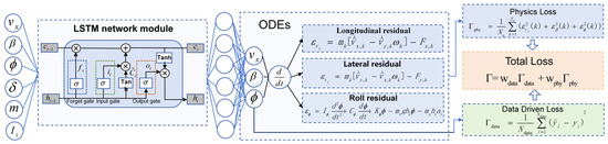
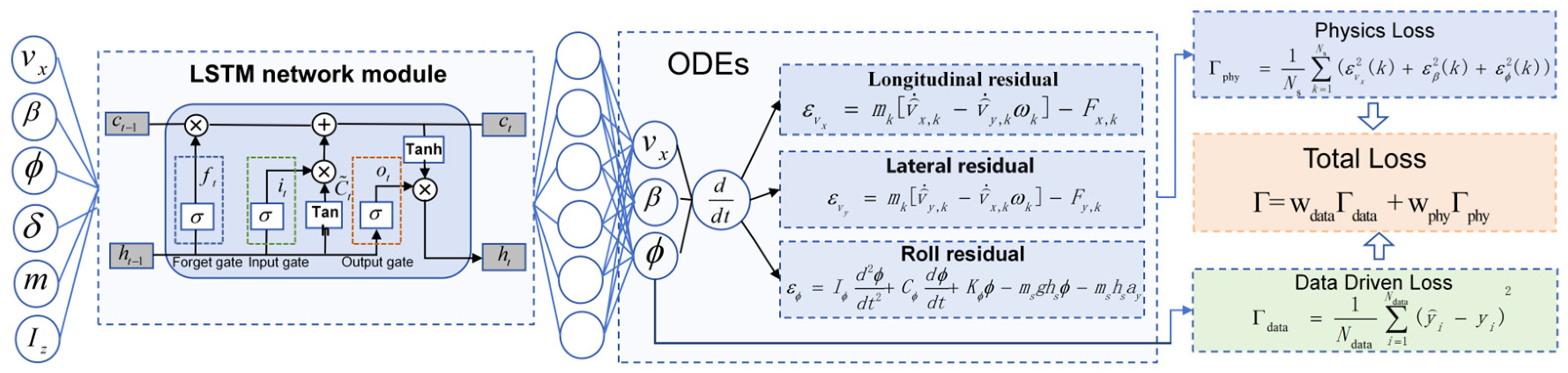
To achieve high precision estimation of critical vehicle dynamic states under complex operating conditions, this paper develops a PINN-based state estimator at the lower layer of a hierarchical collaborative estimation framework. Unlike traditional purely data-driven methods that rely solely on input–output mappings, the proposed PINN incorporates coupled dynamic constraints of longitudinal, lateral, and roll motions into the supervised learning process. This design ensures that the network outputs not only approximate the true states but also satisfy fundamental dynamic equilibrium relationships, thereby improving robustness and generalization across varying operating conditions. The overall framework of the PINN-based vehicle state estimator is illustrated in Figure 3.
Figure 3.
PINN-based vehicle state estimation framework.
Considering the discrete sampling instant , the network input state vector is defined as
where denotes the longitudinal velocity, is the vehicle sideslip angle, is the roll angle, is the front wheel steering angle, is the vehicle mass, and is the yaw moment of inertia. A historical sliding window with length is constructed as the network input, where . Accordingly, the input sequence can be expressed as
The network output is defined as the estimated state at the next sampling instant:
where denotes the neural network parameterized by .
In terms of network architecture, the proposed state estimator consists of a sequence input layer, LSTM hidden layers, and fully connected mapping layers. The forget gate, input gate, and output gate are defined as follows:
where and denote the weight matrices and bias vectors of the corresponding gates, respectively; is the hidden state at the previous time step, and is the input vector at the current time step.
The cell state update and output generation are formulated as follows:
where and denote the learnable weight matrices and bias vectors, respectively; is the hyperbolic tangent activation function, and represents element-wise multiplication.
The total loss function consists of a data supervision loss and a physics residual loss:
where denotes the total loss function, denotes the data supervision loss, and denotes the physics residual loss. and are the weighting coefficients used to balance the supervised loss from measurement data and the unsupervised ODE-based physical residual loss, respectively. In this study, and are set to 0.8 and 0.2, respectively.
The data supervision loss is defined using the mean squared error (MSE) to quantify the deviation between the network outputs and the ground truth state labels:
where denotes the total number of training samples, and represents the ground truth state label of the -th sample.
The physics residual loss is constructed following the general PINN formulation, in which the governing ODE residual is defined as the discrepancy between the state derivative given by the physical model and the time derivative of the network-predicted state:
where is the ODEs of the vehicle dynamics system. Therefore, by substituting the network-predicted states , , and into the vehicle dynamic equations, and by computing their time derivatives, the ODE residuals can be expressed in the form of dynamic equilibrium errors.
The longitudinal residual is obtained from the longitudinal force equilibrium and is used to constrain the evolution of . The lateral residual is obtained from the lateral force equilibrium and constrains , thereby indirectly constraining the sideslip angle . The roll residual is obtained from the roll dynamic equilibrium and is used to constrain the roll response . Accordingly, the physics residuals are formulated as follows:
where , , , and are obtained from CarSim or calculated through the vehicle dynamics model, and denotes the yaw rate. It should be noted that the yaw coupling effect is not ignored in the above residual formulation. Although the yaw dynamic equation is not independently formulated as a separate residual term, the yaw rate enters the longitudinal and lateral residuals through the coupling terms and . In addition, yaw motion also affects the tire slip-angle calculation and tire-force generation. Therefore, the yaw coupling effect is implicitly incorporated into the longitudinal and lateral dynamic residuals.
Furthermore, tire nonlinearities are reflected through the Pacejka tire model adopted in the vehicle dynamics model. The tire forces and used in the residuals are functions of slip ratio, slip angle, and vertical load, rather than being obtained from a simple linear tire stiffness approximation. Load-transfer effects are also included through the dynamic vertical loads of the four wheels. Variations in longitudinal acceleration, lateral acceleration, vehicle mass, center-of-gravity height, wheelbase, and track width affect the tire vertical loads, which further influence the longitudinal and lateral tire forces and eventually enter the physics residuals. Therefore, the selected residuals provide direct constraints on the target states, while yaw coupling, tire nonlinearities, and load-transfer effects are incorporated through the coupled vehicle dynamics model, tire slip-angle relationships, Pacejka tire-force model, and dynamic vertical-load formulation.
Based on the above residuals, the physics-based loss is defined as
Since the lateral residual constraints , it provides a direct physical constraint on the sideslip angle estimation. Therefore, can also be regarded as the sideslip-related dynamic residual.
Based on the MCAUK-PINN framework, the propagation of estimation errors from the upper-layer MCAUKF to the lower-layer PINN can be effectively suppressed. The upper-layer MCAUKF improves the robustness of inertial parameter identification under uncertain noise conditions. However, inaccurate estimation of vehicle mass or yaw moment of inertia may still lead to the following issues: First, these inertial parameters are embedded in the longitudinal, lateral, and roll dynamics constraints, and their deviations introduce systematic errors into the physical residuals. Second, the identified inertial parameters also serve as input features to the lower-layer PINN, and their estimation errors directly disturb the input–output mapping learned by the network. Third, due to the use of a historical sliding window input structure in the PINN, persistent parameter estimation biases propagate along the time sequence, thereby affecting subsequent state predictions. To mitigate the aforementioned error propagation, the identified inertial parameters are introduced as soft physical priors rather than hard constraints in the lower-layer design. The total loss function consists of both data supervision loss and physical residual loss, with the data supervision loss assigned a dominant weight to prevent residual errors caused by parameter inaccuracies from dominating the training process. Furthermore, the historical sliding window input helps attenuate instantaneous parameter fluctuations and enhances temporal robustness. Consequently, excessive error propagation from the upper layer to the lower layer can be suppressed to a certain extent.
4. Simulation and Analysis
4.1. Dataset Construction
In this study, the dataset for training and testing the PINN-based state estimator was generated using a CarSim-MATLAB/Simulink co-simulation platform. CarSim is used as the high-fidelity virtual vehicle model to provide vehicle body dynamics, tire-road interaction, road adhesion conditions, load configuration, and reference vehicle states. The co-simulation platform was established using CarSim 2023.1 and MATLAB/Simulink R2023b. CarSim 2023.1 was used as the high-fidelity virtual vehicle model, while MATLAB/Simulink R2023b was used for signal acquisition and processing, implementation of the proposed MCAUKF-PINN estimator, and construction of the training and testing datasets. The vehicle parameters in CarSim are configured according to Table 1. To ensure sufficient coverage of vehicle operating conditions, simulation experiments were conducted under different vehicle speeds, road adhesion coefficients, load conditions, and maneuvering scenarios, including slalom, double lane change, and emergency lane change maneuvers. The vehicle speed ranged from 20 to 120 km/h with an interval of 5 km/h; the road adhesion coefficient ranged from 0.3 to 0.9 with an interval of 0.1; and the vehicle mass was set from 1400 to 1900 kg. For load-varying conditions, the vehicle mass, center-of-gravity position, vertical load distribution, and yaw moment of inertia were updated in CarSim according to the prescribed load configuration. All simulation data were collected at a sampling frequency of 1 kHz and divided into training and testing datasets at a ratio of 7:3. The network input samples were constructed using a 20 ms sliding time window.
4.2. State Estimation Results
To systematically evaluate the effectiveness and robustness of the proposed hierarchical joint estimation framework under varying load conditions, road adhesion levels, and steering inputs, two representative scenarios are considered for simulation-based validation: a high adhesion, low-speed double-lane change (DLC) maneuver and a low-adhesion, high-speed serpentine maneuver. In addition, random noise is injected into the measurement channels to emulate the non-ideal sensing conditions encountered by onboard sensors in complex real-world environments.
Scenario 1 corresponds to a low-speed DLC maneuver under high-friction conditions, with a vehicle speed of 60 km/h, a road friction coefficient of 0.8, and a vehicle mass of 1870 kg. Scenario 2 corresponds to a high-speed slalom maneuver under low friction conditions, with an initial vehicle speed of 80 km/h, a road friction coefficient of 0.3, and a vehicle mass of 1560 kg. The two scenarios are designed to evaluate the estimation performance of the proposed method under high-adhesion complex maneuvering conditions and low-adhesion strongly coupled dynamic conditions, respectively. Additional loads change the total vehicle mass and shift the center-of-gravity position, thereby leading to variations in the yaw moment of inertia according to the parallel-axis theorem. Meanwhile, the migration of the center of gravity and the variation in sprung mass further affect the vertical load distribution among the four wheels, tire-force generation, and the yaw and roll responses of the vehicle. Therefore, in this study, the moments of inertia in the two scenarios are automatically updated in CarSim under the prescribed load mass and load distribution conditions.
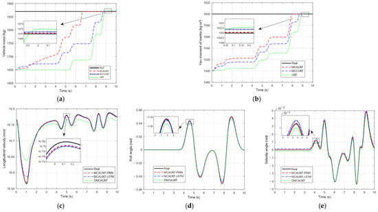
To verify the effectiveness of the proposed hierarchical collaborative estimation framework, a comparative analysis is conducted from two perspectives: upper-layer inertial parameter identification and lower-layer key state estimation. For the upper layer, MCAUKF, MCCUKF, and UKF are, respectively, employed for the online identification of and , while maintaining the same structure and training settings for the lower-layer state estimator. This comparison is intended to evaluate the differences among the three methods in terms of convergence rate, steady-state accuracy, and robustness. For the lower layer, with the upper-layer parameter estimator fixed as MCAUKF, three state estimation methods, PINN, LSTM, and MCAUKF, are constructed, yielding three comparison schemes: MCAUKF-PINN, MCAUKF-LSTM, and D-MCAUKF. These methods are used to estimate , , and . To quantitatively characterize estimation performance, root mean square error (RMSE) and mean absolute error (MAE) are adopted as evaluation metrics. The results are used to comprehensively assess the performance advantages of the proposed MCAUKF-PINN hierarchical collaborative estimation framework.
4.2.1. Simulation Results Under DLC Conditions on Dry Asphalt Road Surface
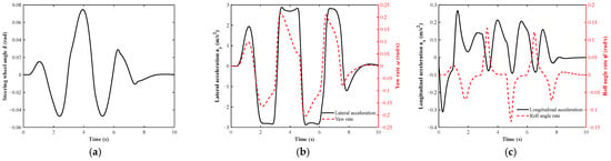
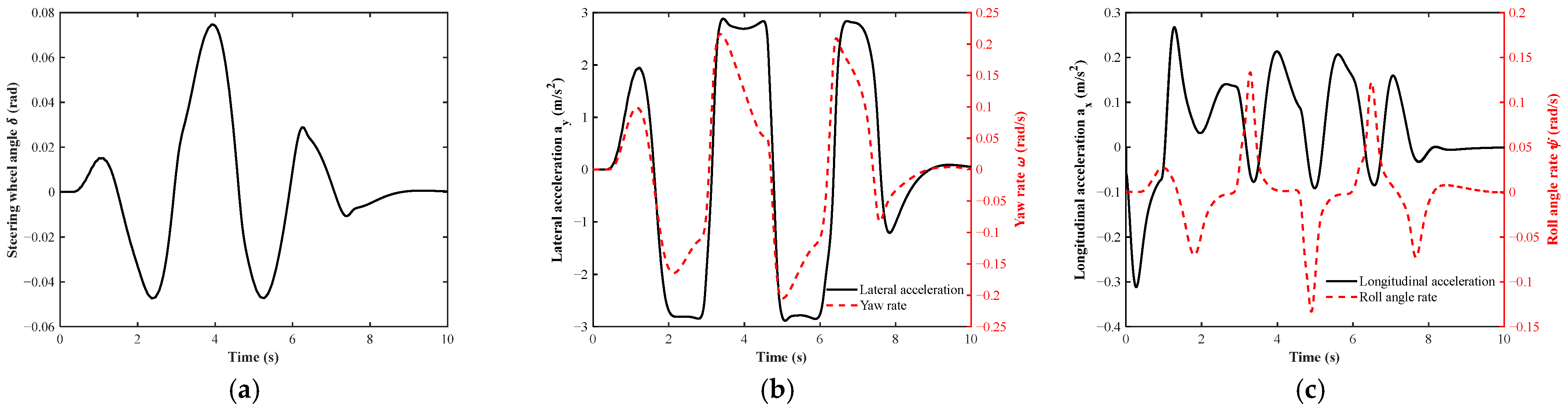
The sensor measurement signals under the double lane change condition on a dry asphalt road surface are shown in Figure 4. Figure 4a presents the steering wheel angle input, which provides sufficient excitation for the lateral and yaw motions of the vehicle. Figure 4b shows the lateral acceleration and yaw rate responses. Both signals vary consistently with the steering wheel angle input, indicating that the double lane change maneuver induces significant lateral–yaw coupling. Figure 4c presents the longitudinal acceleration and roll rate responses. The roll rate changes noticeably during the rapid reverse steering phases, reflecting the vehicle body roll motion caused by lateral load transfer. These signals are closely related to the longitudinal, lateral, and roll coupled dynamics considered in the PINN physical residual constraints proposed in this study. Therefore, the sensor measurement signals shown in Figure 4 not only describe the dynamic characteristics of the vehicle under the double lane change condition, but also provide important input information for inertial parameter identification and key state estimation in the proposed hierarchical MCAUKF-PINN framework.
Figure 4.
Sensor measurement inputs under the DLC condition: (a) steering angle; (b) lateral acceleration and yaw rate; (c) longitudinal acceleration and roll rate.
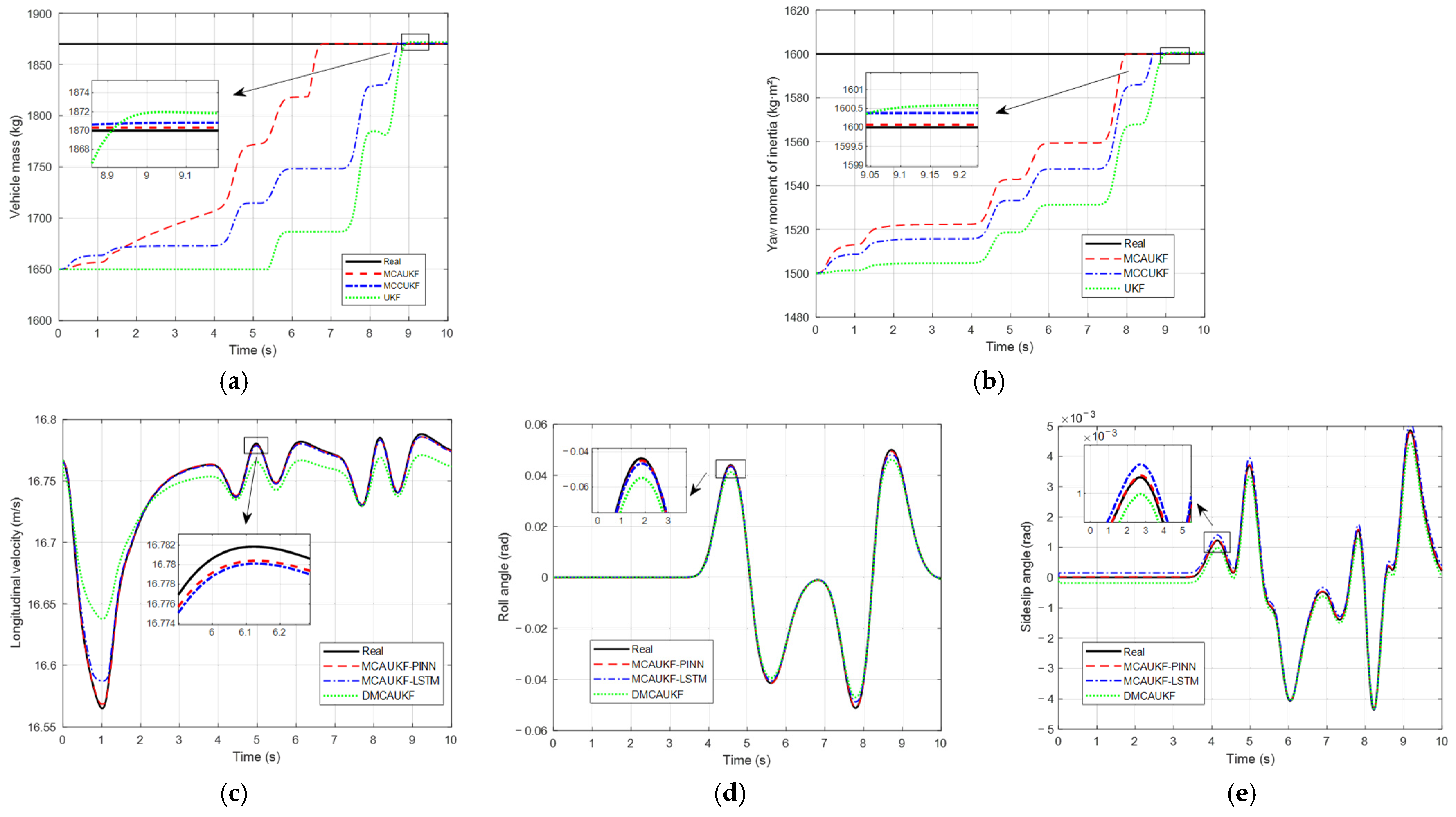
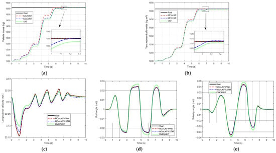
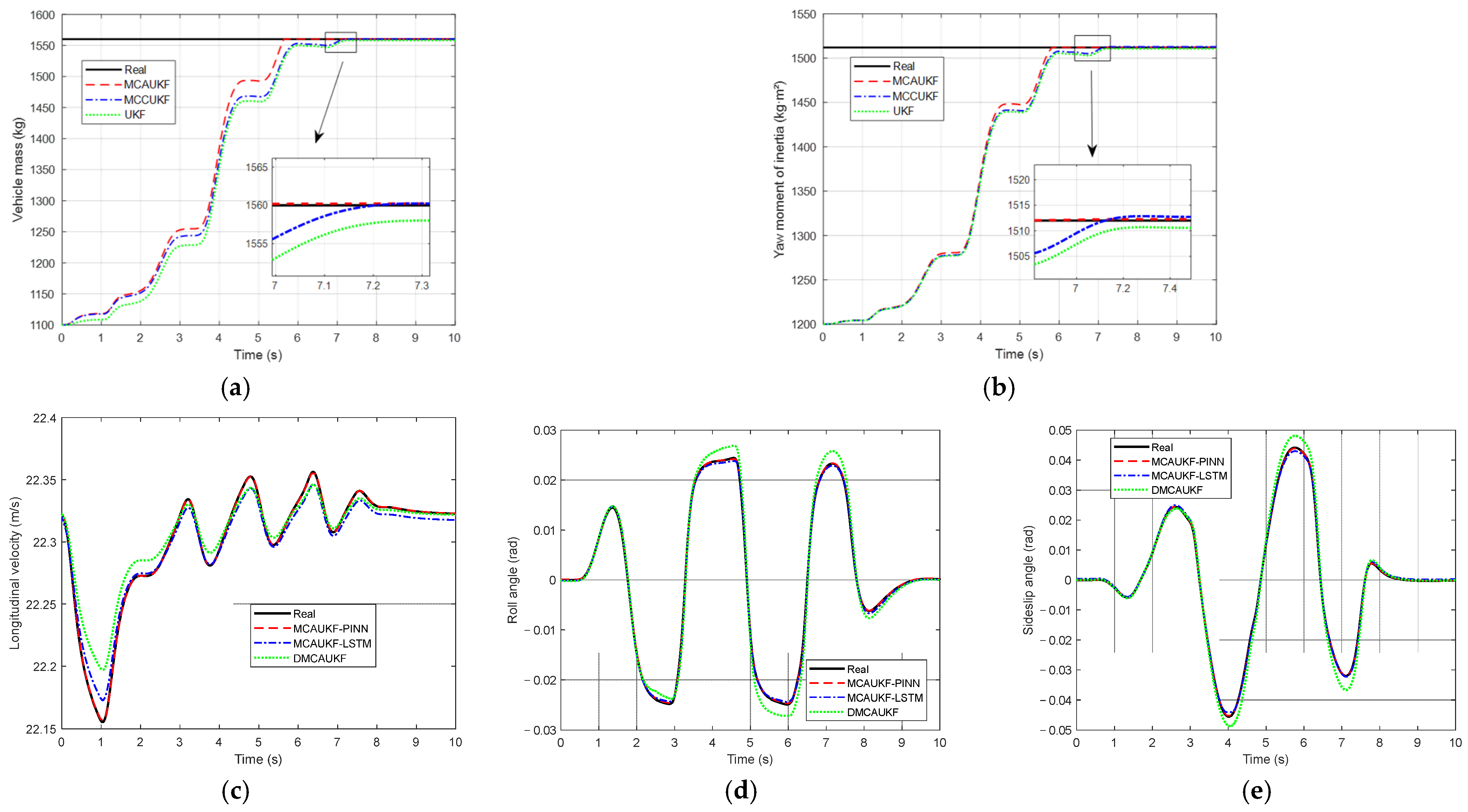
To validate the effectiveness of the upper-layer MCAUKF for inertial parameter identification, it is compared with MCCUKF and UKF under identical initial conditions and noise settings. As shown in Figure 5a,b, under the DLC condition, all three methods converge toward the true values of and , but clear differences are observed in convergence speed and steady-state accuracy. Among them, MCAUKF exhibits the fastest convergence and the smallest steady-state error. Although MCCUKF improves upon UKF, it still suffers from response lag and local bias accumulation. By contrast, UKF shows the slowest convergence and the largest steady-state deviation. This superior performance of MCAUKF is mainly attributed to the simultaneous incorporation of the MCC and the adaptive noise statistics adjustment mechanism, which enables it to suppress uncertain noise and adapt online to variations in noise statistics. Quantitative results show that, for identification, MCAUKF reduces the RMSE and MAE by 28.81% and 40.68%, respectively, compared with UKF, and further reduces the MAE by 26.08% compared with MCCUKF. For identification, MCAUKF reduces the RMSE and MAE by 21.41% and 26.43%, respectively, relative to UKF, and by 9.26% and 12.44%, respectively, relative to MCCUKF. These results demonstrate that MCAUKF can achieve more accurate and robust inertial parameter identification, thereby providing more reliable parameter priors for the lower-layer state estimation module.
Figure 5.
Estimation results for the low-speed DLC maneuver on a dry asphalt road surface: (a) vehicle mass; (b) yaw moment of inertia; (c) longitudinal velocity; (d) roll angle; (e) sideslip angle.
Figure 5c–e present the comparative estimation results of , , an , respectively. Overall, MCAUKF-PINN achieves the best tracking performance throughout the DLC maneuver, maintaining high estimation accuracy even during rapid dynamic transitions. In contrast, D-MCAUKF exhibits noticeable deviations and slight lag under strong steering coupling, indicating that purely model-driven methods are sensitive to noise uncertainty and model mismatch. Although MCAUKF-LSTM improves the estimation results to some extent, local biases remain in certain dynamic intervals, suggesting that purely data-driven methods without explicit physical constraints still have limited robustness under complex operating conditions. By embedding the residuals derived from coupled longitudinal, lateral, and roll dynamics into the network training process, and by incorporating inertial parameter priors provided by the upper layer MCAUKF to constrain state evolution, PINN can capture vehicle dynamic characteristics more accurately under complex conditions, suppress unreasonable state deviations, and improve estimation accuracy.
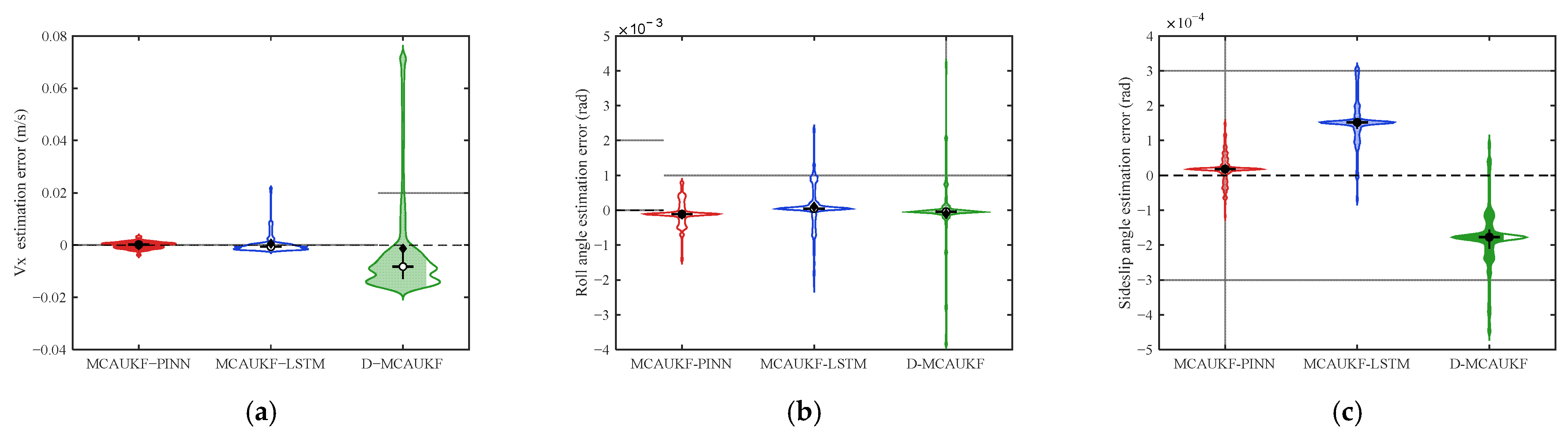
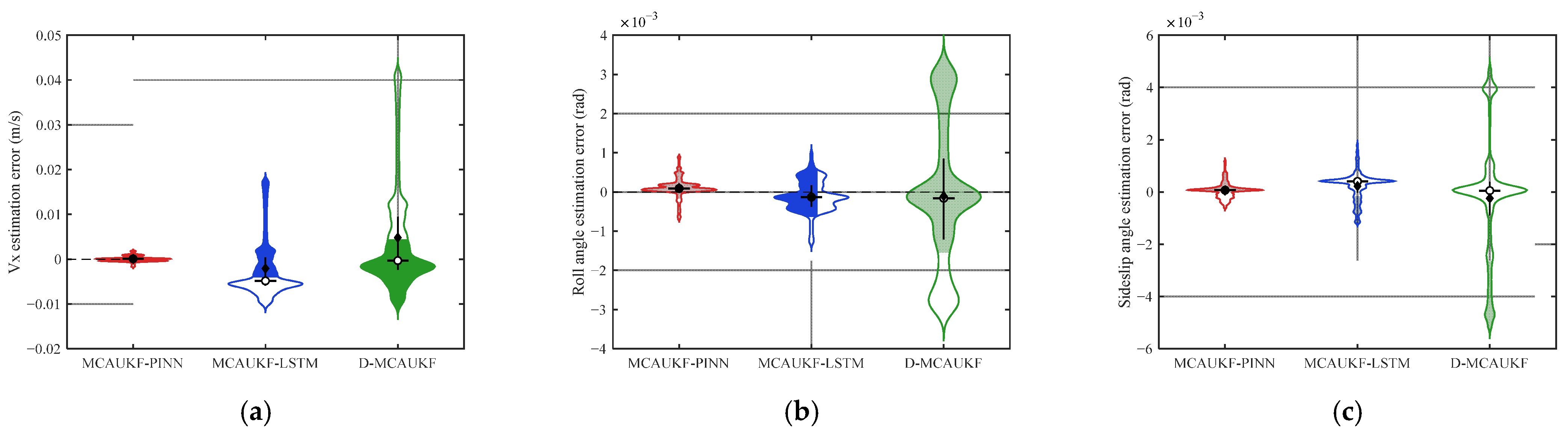
The quantitative results in Table 2 further confirm the superiority of MCAUKF-PINN. For longitudinal velocity estimation, its RMSE and MAE are reduced by 93.74% and 92.70%, respectively, relative to D-MCAUKF, and by 68.49% and 51.06%, respectively, relative to MCAUKF-LSTM. For roll angle estimation, the corresponding reductions are 70.19% and 61.58% compared with D-MCAUKF, and 41.57% and 33.10% compared with MCAUKF-LSTM. For sideslip angle estimation, the RMSE and MAE are reduced by 77.86% and 81.39%, respectively, relative to D-MCAUKF, and by 72.72% and 77.44%, respectively, relative to MCAUKF-LSTM. Figure 6 further shows that MCAUKF-PINN yields the most concentrated error distributions, with the mean and median values closest to zero, indicating superior estimation accuracy and robustness. Overall, MCAUKF-PINN significantly improves the accuracy and robustness of key state estimation under complex driving conditions.
Table 2.
State estimation results for the low-speed DLC maneuver on a dry asphalt road surface.
Figure 6.
Estimation error distributions for the low-speed DLC maneuver on a dry asphalt road surface: (a) estimation error; (b) estimation error; (c) estimation error.
Overall, under the DLC condition on a dry asphalt road, the proposed MCAUKF-PINN hierarchical joint estimation framework achieves the best overall performance in the online estimation of both inertial parameters and key vehicle states. MCAUKF improves the convergence speed and steady-state accuracy of and , while PINN significantly enhances the estimation accuracy of , , and . These results indicate that MCAUKF-PINN provides an effective approach for improving the collaborative estimation performance of vehicle inertial parameters and dynamic states.
4.2.2. Simulation Results Under Slalom Maneuvers on a Wet Low-Friction Road Surface
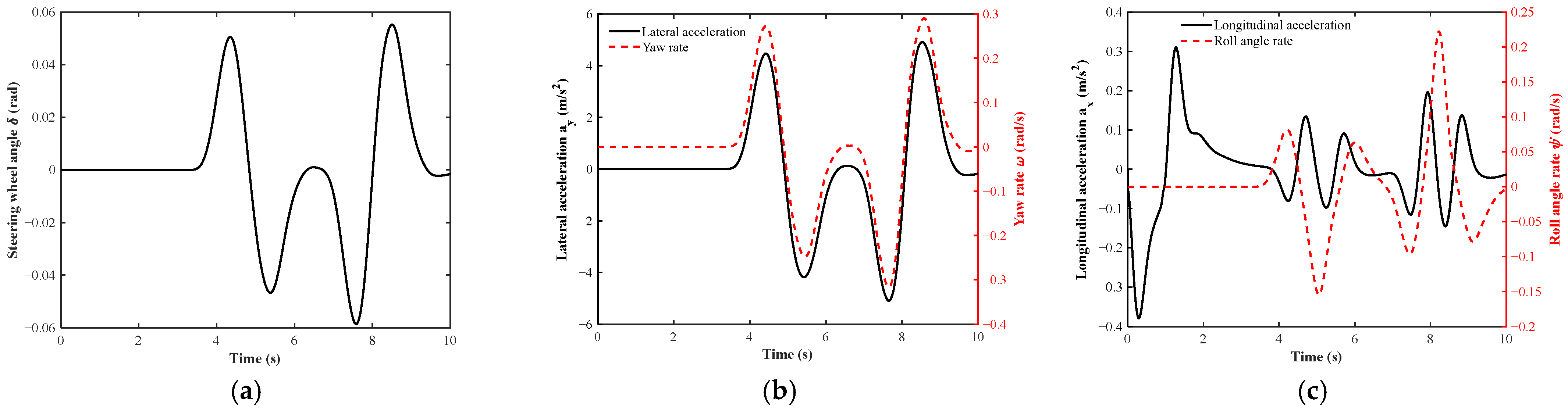
The sensor measurement signals under the slalom maneuver on a wet, low-friction road surface are shown in Figure 7. Figure 7a presents the steering wheel angle input. The continuous steering reversals in the slalom maneuver provide sufficient excitation for the lateral and yaw motions of the vehicle. Figure 7b shows the lateral acceleration and yaw rate responses. Both signals vary significantly with the steering wheel angle input, indicating strong lateral–yaw coupling under the low-friction road condition. Figure 7c presents the longitudinal acceleration and roll rate responses. The longitudinal acceleration fluctuates because of the coupling between longitudinal and lateral dynamics, while the roll rate changes noticeably during rapid steering reversals, reflecting the vehicle body roll motion caused by lateral load transfer. Figure 7 not only describes the dynamic characteristics of the vehicle under the wet low-friction slalom maneuver, but also provides important input information for inertial parameter identification and key state estimation in the proposed hierarchical MCAUKF-PINN framework.
Figure 7.
Sensor measurement inputs under the slalom maneuver condition: (a) steering angle; (b) lateral acceleration and yaw rate; (c) longitudinal acceleration and roll rate.
Under the wet-road serpentine steering condition, the vehicle undergoes continuous rapid steering reversals at an initial speed of 80 km/h, resulting in strong coupling among longitudinal, lateral, and yaw dynamics and thus posing greater challenges for inertial parameter identification and key state estimation. The simulation results show that, in the online identification of and , MCAUKF consistently outperforms MCCUKF and UKF in terms of convergence speed, transient error, and steady-state accuracy. Quantitatively, for vehicle , compared with UKF, MCAUKF reduces the RMSE and MAE by 4.69% and 8.35%, respectively; compared with MCCUKF, the corresponding reductions are 1.77% and 4.54%. For estimation, MCAUKF reduces the RMSE and MAE by 6.91% and 14.08%, respectively, relative to UKF, and by 1.39% and 4.33%, respectively, relative to MCCUKF. Overall, MCAUKF achieves the best performance, indicating that the proposed adaptive robust filtering framework can still stably improve inertial parameter identification accuracy under strongly coupled serpentine maneuvering conditions on low-adhesion roads.
Figure 8c–e compare the estimation results of , and . Overall, under high-speed slalom conditions on a wet and slippery road surface, MCAUKF-PINN consistently delivers the best tracking performance, maintaining close agreement with the true states even under continuous steering reversals and strongly coupled dynamic conditions. In contrast, D-MCAUKF exhibits significant amplitude errors and lag across multiple peak-to-trough intervals, indicating that purely model-driven methods are sensitive to noise disturbances and model mismatch. Although MCAUKF-LSTM improves the estimation results to some extent, noticeable deviations remain over certain local intervals, reflecting the limited robustness of purely data-driven methods without explicit physical constraints under complex operating conditions. By embedding the residuals of coupled longitudinal, lateral, and roll dynamics into the training process and constraining state evolution with inertial parameter priors from the upper layer, PINN can characterize the strongly coupled vehicle dynamics under serpentine maneuvers more accurately.
Figure 8.
Estimation results for high-speed slalom maneuver on a wet concrete surface. (a) Vehicle mass; (b) yaw moment of inertia; (c) longitudinal velocity; (d) roll angle; (e) sideslip angle.
The quantitative evaluation results in Table 3 indicate that the proposed MCAUKF-PINN method maintains a significant overall advantage under high-speed slalom maneuvers on wet roads. Specifically, for estimation, the RMSE and MAE of MCAUKF-PINN are reduced by 93.76% and 92.02% compared to D-MCAUKF, and by 88.00% and 88.43% compared to MCAUKF-LSTM. For roll angle estimation, compared with D-MCAUKF, the RMSE and MAE of MCAUKF–PINN are reduced by 83.54% and 85.30%, respectively; compared with MCAUKF–LSTM, the corresponding reductions are 35.44% and 44.01%, respectively. For sideslip angle estimation, MCAUKF–PINN again achieves the best performance, with RMSE and MAE reductions of 87.0% and 85.86%, respectively, relative to D-MCAUKF, and 48.74% and 56.06%, respectively, relative to MCAUKF–LSTM.
Table 3.
State estimation results for the high-speed slalom maneuver on a wet concrete road surface.
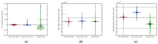
The violin plots in Figure 9 further demonstrate that MCAUKF-PINN yields the most concentrated error distributions across all three key states, with both the mean and median closest to zero, indicating superior estimation accuracy and robustness. Overall, the proposed MCAUKF-PINN hierarchical collaborative estimation framework significantly improves the accuracy and robustness of key state estimation under complex operating conditions.
Figure 9.
Estimation error distributions for the high-speed slalom maneuver on a wet concrete road surface. (a) estimation error; (b) roll angle estimation error; (c) sideslip angle estimation error.
In summary, the MCAUKF-PINN hierarchical joint estimation method enables robust online identification of inertial parameters and high-precision estimation of key states under highly nonlinear and strongly coupled serpentine maneuvering conditions, thereby further validating the effectiveness and robustness of the proposed framework under complex operating conditions.
5. Conclusions and Future Work
This paper proposes a hierarchical collaborative estimation method that integrates MCAUKF-PINN for inertial parameter identification and key dynamic state estimation in distributed drive electric vehicles. To address the distinct task characteristics of inertial parameter identification and dynamic state estimation, the joint estimation problem is decomposed into two layers: upper-layer inertial parameter identification and lower-layer state estimation. In the upper layer, MCAUKF is employed to achieve robust online identification of vehicle mass and moment of inertia. In the lower layer, a PINN incorporating dynamic constraints is developed to enable high precision estimation of longitudinal velocity, sideslip angle, and roll angle. Based on the CarSim–Simulink co-simulation platform, the proposed method was validated under two representative scenarios: high-friction, low-speed lane change conditions and low-friction, high-speed serpentine conditions. Taking the latter as an example, for vehicle mass estimation, the RMSE and MAE of MCAUKF were reduced by 4.69% and 8.35%, respectively, compared with those of UKF; for rotational inertia estimation, the corresponding reductions were 6.91% and 14.08%, respectively. In terms of key state estimation, the RMSE and MAE of velocity estimation achieved by MCAUKF-PINN were reduced by 93.76% and 92.02%, respectively, relative to D-MCAUKF. For roll angle estimation, the corresponding reductions were 83.54% and 85.30%, respectively; for sideslip angle estimation, they were 87.0% and 85.86%, respectively. The above results demonstrate that the proposed method can effectively improve inertial parameter identification accuracy, enhance key state estimation performance, and strengthen overall estimation robustness under complex operating conditions.
The proposed PINN-based estimator has potential for cross-vehicle extension because its physics-informed loss is constructed from general longitudinal, lateral, and roll dynamic relationships. Moreover, the upper-layer MCAUKF identifies key inertial parameters online and introduces them into the PINN physical residuals as time-varying priors, reducing dependence on fixed nominal parameters. However, differences in vehicle structure, tire characteristics, actuator dynamics, and sensor configurations may affect dynamic responses and signal distributions. Therefore, when applying the framework to other vehicle types, vehicle-specific parameters should be updated, and transfer learning, fine-tuning, or retraining with target-vehicle data may be required. In this study, the proposed method is validated using only one vehicle model under different vehicle speeds, road adhesion coefficients, load conditions, and maneuvering scenarios. Therefore, its cross-vehicle generalization capability has not yet been fully verified and still requires further investigation. Future work will focus on constructing multi-vehicle datasets and conducting hardware-in-the-loop tests and real-vehicle experiments on different vehicle platforms to further evaluate and improve the generalization capability, real-time performance, robustness, and engineering applicability of the proposed method. In particular, we will further integrate the proposed MCAUKF-PINN framework with battery management systems, motor drive systems, power electronic converters, and thermal management models to systematically evaluate its potential role in enhancing energy efficiency, powertrain operational safety, and thermal reliability. Moreover, adaptive weighting strategies for physical constraints and more efficient temporal network architectures will be explored to enhance the practical applicability of the proposed framework under real-world operating conditions.
Author Contributions
Methodology, software, and writing—original draft and editing, H.W.; validation and writing—review and editing, H.Z.; investigation and data curation, C.G., J.M. and Y.L.; supervision and funding acquisition, Y.Z. All authors have read and agreed to the published version of the manuscript.
Funding
This work was supported by the National Natural Science Foundation of China (Grant No. 52402522), the Key Research and Development Program of Shanxi Province (Grant No. 202502010101013), the 2025 Annual Postgraduate Academic Innovation Program of Shanxi Province (Grant No. 2025XS121), and the 2025 Annual Postgraduate Practical Innovation Project of Shanxi Province (Grant No. 2025SJ026).
Data Availability Statement
The data used in this analysis are publicly available and access is provided in the text.
Conflicts of Interest
The authors declare no conflicts of interest.
References
- Zhang, Y.; Ai, Z.; Chen, J.; You, T.; Du, C.; Deng, L. Energy-Saving Optimization and Control of Autonomous Electric Vehicles With Considering Multiconstraints. IEEE Trans. Cybern. 2022, 52, 10869–10881. [Google Scholar] [CrossRef] [Scilit]
- Liang, J.; Feng, J.; Fang, Z.; Lu, Y.; Yin, G.; Mao, X.; Wu, J.; Wang, F. An Energy-Oriented Torque-Vector Control Framework for Distributed Drive Electric Vehicles. IEEE Trans. Transp. Electrifc. 2023, 9, 4014–4031. [Google Scholar] [CrossRef] [Scilit]
- Zhao, K.; Fan, X.; Huang, Z.; Yu, X.; Wang, L.; Peng, J. A Review of Drive Torque Distribution Control for Distributed Drive Electric Vehicles. Proc. Inst. Mech. Eng. Part D J. Automob. Eng. 2025, 239, 5291–5315. [Google Scholar] [CrossRef] [Scilit]
- Xue, Z.; Cheng, S.; Li, L.; Zhong, Z.; Mu, H. A Robust Unscented M-Estimation-Based Filter for Vehicle State Estimation With Unknown Input. IEEE Trans. Veh. Technol. 2022, 71, 6119–6130. [Google Scholar] [CrossRef] [Scilit]
- Lin, J.; Zou, T.; Su, L.; Zhang, F.; Zhang, Y. Optimal Coordinated Control of Active Front Steering and Direct Yaw Moment for Distributed Drive Electric Bus. Machines 2023, 11, 640. [Google Scholar] [CrossRef] [Scilit]
- Katriniok, A.; Abel, D. Adaptive EKF-Based Vehicle State Estimation With Online Assessment of Local Observability. IEEE Trans. Contr. Syst. Technol. 2016, 24, 1368–1381. [Google Scholar] [CrossRef] [Scilit]
- Li, H.; Zhang, R.; Shi, P.; Xiao, P.; Zheng, K.; Qiu, T. State Parameters Estimation for Distributed Drive Electric Vehicle Based on PMSMs’ Sensorless Control. IEEE Sens. J. 2024, 24, 24054–24069. [Google Scholar] [CrossRef] [Scilit]
- Song, R.; Fang, Y. Vehicle State Estimation for INS/GPS Aided by Sensors Fusion and SCKF-Based Algorithm. Mech. Syst. Signal Process. 2021, 150, 107315. [Google Scholar] [CrossRef] [Scilit]
- Fan, R.; Li, G.; Wu, Y. State Estimation of Distributed Drive Electric Vehicle Based on Adaptive Kalman Filter. Sustainability 2023, 15, 13446. [Google Scholar] [CrossRef] [Scilit]
- Li, R.; Hong, J.; Zhang, H.; Chen, X. Data-Driven Battery State of Health Estimation Based on Interval Capacity for Real-World Electric Vehicles. Energy 2022, 257, 124771. [Google Scholar] [CrossRef] [Scilit]
- Oh, S.; Kim, J.; Moon, I. Hybrid Data-Driven Deep Learning Model for State of Charge Estimation of Li-Ion Battery in an Electric Vehicle. J. Energy Storage 2024, 97, 112887. [Google Scholar] [CrossRef] [Scilit]
- Yuan, H.; Song, X. Adaptive Adjustment of Noise Covariance for Vehicle State Estimation Under Packet Dropping. Int. J. Control Autom. Syst. 2023, 21, 3642–3649. [Google Scholar] [CrossRef] [Scilit]
- Zhu, J.; Wang, Z.; Zhang, L.; Zhang, W. State and Parameter Estimation Based on a Modified Particle Filter for an In-Wheel-Motor-Drive Electric Vehicle. Mech. Mach. Theory 2019, 133, 606–624. [Google Scholar] [CrossRef] [Scilit]
- Liu, Y.; Ji, X.; Yang, K.; He, X.; Na, X.; Liu, Y. Finite-Time Optimized Robust Control with Adaptive State Estimation Algorithm for Autonomous Heavy Vehicle. Mech. Syst. Signal Process. 2020, 139, 106616. [Google Scholar] [CrossRef] [Scilit]
- Huang, C.; Tang, W.; Wang, J.; Zhang, Z. An Improved Adaptive Car-Following Model Based on the Unscented Kalman Filter for Vehicle Platoons’ Speed Control. Machines 2025, 13, 569. [Google Scholar] [CrossRef] [Scilit]
- Ren, H.; Chen, S.; Liu, G.; Zheng, K. Vehicle State Information Estimation with the Unscented Kalman Filter. Adv. Mech. Eng. 2014, 6, 589397. [Google Scholar] [CrossRef] [Scilit]
- Wang, Y.; Li, Y.; Zhao, Z. State Parameter Estimation of Intelligent Vehicles Based on an Adaptive Unscented Kalman Filter. Electronics 2023, 12, 1500. [Google Scholar] [CrossRef] [Scilit]
- Zhang, F.; Feng, J.; Qi, D.; Liu, Y.; Shao, W.; Qi, J.; Lin, Y. Joint Estimation of Vehicle State and Parameter Based on Maximum Correntropy Adaptive Unscented Kalman Filter. Int. J. Automot. Technol. 2023, 24, 1553–1566. [Google Scholar] [CrossRef] [Scilit]
- Zhang, Y.; Song, X.; Liu, Z. Maximum Correntropy Unbiased Minimum-Variance Filter. Signal Process. 2024, 219, 109405. [Google Scholar] [CrossRef] [Scilit]
- Ghosh, A.; Honoré, A.; Chatterjee, S. DANSE: Data-Driven Non-Linear State Estimation of Model-Free Process in Unsupervised Learning Setup. IEEE Trans. Signal Process. 2024, 72, 1824–1838. [Google Scholar] [CrossRef] [Scilit]
- Jafari, S.; Byun, Y.-C. Efficient State of Charge Estimation in Electric Vehicles Batteries Based on the Extra Tree Regressor: A Data-Driven Approach. Heliyon 2024, 10, e25949. [Google Scholar] [CrossRef] [Scilit] [PubMed]
- Hossain Lipu, M.S.; Hannan, M.A.; Hussain, A.; Ayob, A.; Saad, M.H.M.; Karim, T.F.; How, D.N.T. Data-Driven State of Charge Estimation of Lithium-Ion Batteries: Algorithms, Implementation Factors, Limitations and Future Trends. J. Clean. Prod. 2020, 277, 124110. [Google Scholar] [CrossRef] [Scilit]
- Xing, Y.; Lv, C. Dynamic State Estimation for the Advanced Brake System of Electric Vehicles by Using Deep Recurrent Neural Networks. IEEE Trans. Ind. Electron. 2020, 67, 9536–9547. [Google Scholar] [CrossRef] [Scilit]
- Kong, D.; Wen, W.; Zhao, R.; Lv, Z.; Liu, K.; Liu, Y.; Gao, Z. Vehicle Lateral Velocity Estimation Based on Long Short-Term Memory Network. World Electr. Veh. J. 2021, 13, 1. [Google Scholar] [CrossRef] [Scilit]
- Zhang, Y.; Xu, N.; Yin, Z.; Guo, K. A Direct Tire Capacity Estimation Method Using Deep Learning With On-Board Sensor Signals. IEEE Trans. Veh. Technol. 2025, 74, 8529–8543. [Google Scholar] [CrossRef] [Scilit]
- Chen, J.; Pan, W.; Cao, T.; Qian, Z.; Zhang, L.; Chen, X.; Chen, H. Auxiliary-Enhanced Neural Networks for Electric Vehicle Dynamics: Advancing Tire Force and State Estimation during Wheel Slip. Control. Eng. Pract. 2025, 165, 106550. [Google Scholar] [CrossRef] [Scilit]
- Bertipaglia, A.; Alirezaei, M.; Happee, R.; Shyrokau, B. An Unscented Kalman Filter-Informed Neural Network for Vehicle Sideslip Angle Estimation. IEEE Trans. Veh. Technol. 2024, 73, 12731–12746. [Google Scholar] [CrossRef] [Scilit]
- Li, Q.; Zhang, B.; He, H.; Wang, Y.; He, D.; Mo, S. A Hybrid Physics-Data Driven Approach for Vehicle Dynamics State Estimation. Mech. Syst. Signal Process. 2025, 225, 112249. [Google Scholar] [CrossRef] [Scilit]
- Tan, C.; Cai, Y.; Wang, H.; Sun, X.; Chen, L. Vehicle State Estimation Combining Physics-Informed Neural Network and Unscented Kalman Filtering on Manifolds. Sensors 2023, 23, 6665. [Google Scholar] [CrossRef] [Scilit]
- Lim, H.; Lee, J.W.; Boyack, J.; Choi, J.B. EV-PINN: A Physics-Informed Neural Network for Predicting Electric Vehicle Dynamics. arXiv 2024, arXiv:2411.14691. [Google Scholar]
- Wang, Z.; Chen, C.; Jiang, Q.; Zheng, H.; Kaku, C. State Estimation of Drive-by-Wire Chassis Vehicle Based on Dual Unscented Particle Filter Algorithm. Chin. J. Mech. Eng. 2024, 37, 11. [Google Scholar] [CrossRef] [Scilit]
- Gadola, M.; Chindamo, D.; Romano, M.; Padula, F. Development and Validation of a Kalman Filter-Based Model for Vehicle Slip Angle Estimation. Veh. Syst. Dyn. 2014, 52, 68–84. [Google Scholar] [CrossRef] [Scilit]
- Rozyn, M.; Zhang, N. A Method for Estimation of Vehicle Inertial Parameters. Veh. Syst. Dyn. 2010, 48, 547–565. [Google Scholar] [CrossRef] [Scilit]
- Jin, X.; Yang, J.; Li, Y.; Zhu, B.; Wang, J.; Yin, G. Online Estimation Ofinertial Parameter for Lightweight Electric Vehicle Using Dual Unscented Kalman Filter Approach. IET Intell. Trans. Syst. 2020, 14, 412–422. [Google Scholar] [CrossRef] [Scilit]
- Lin, C.; Gong, X.; Xiong, R.; Cheng, X. A Novel H∞ and EKF Joint Estimation Method for Determining the Center of Gravity Position of Electric Vehicles. Appl. Energy 2017, 194, 609–616. [Google Scholar] [CrossRef] [Scilit]
- Cheng, C.; Cebon, D. Parameter and State Estimation for Articulated Heavy Vehicles. Veh. Syst. Dyn. 2011, 49, 399–418. [Google Scholar] [CrossRef] [Scilit]
- Wan, W.; Feng, J.; Song, B.; Li, X. Huber-Based Robust Unscented Kalman Filter Distributed Drive Electric Vehicle State Observation. Energies 2021, 14, 750. [Google Scholar] [CrossRef] [Scilit]
- Huang, X.; Wang, J. Real-Time Estimation of Center of Gravity Position for Lightweight Vehicles Using Combined AKF–EKF Method. IEEE Trans. Veh. Technol. 2014, 63, 4221–4231. [Google Scholar] [CrossRef] [Scilit]

Disclaimer/Publisher’s Note: The statements, opinions and data contained in all publications are solely those of the individual author(s) and contributor(s) and not of MDPI and/or the editor(s). MDPI and/or the editor(s) disclaim responsibility for any injury to people or property resulting from any ideas, methods, instructions or products referred to in the content. |
© 2026 by the authors. Licensee MDPI, Basel, Switzerland. This article is an open access article distributed under the terms and conditions of the Creative Commons Attribution (CC BY) license.