Enhanced Dipole Model-Based Magnetic Disturbance Compensation Using Magnetometer Arrays

Abstract

Magnetometers are widely used in robotics and localization systems but are susceptible to magnetic disturbances generated by nearby ferromagnetic objects, which degrade their accuracy. Traditional calibration methods often fail in dynamic environments, such as those encountered by mobile robots. This paper investigates a dipole model-based disturbance compensation method using a magnetometer array with increased sensor density, extending prior configurations with fewer sensors. The method leverages a detection system to locate disturbing objects, models them as magnetic dipoles, and estimates their parameters through optimization. Experimental validation was performed using magnetic fingerprints of metallic objects in multiple configurations. The results show that increasing sensor density significantly improves compensation performance, reducing magnetic field errors to below 6.64 μT and heading errors to 0.31 rad in most scenarios. In low-to-moderate disturbance scenarios, the four-sensor array achieved heading error improvements of approximately 13% compared to the uncompensated case. In contrast, the proposed nine-sensor array achieved improvements exceeding 50%. In highly complex scenarios involving multiple overlapping disturbances, performance degrades, highlighting limitations of the dipole-based model. These results indicate that increasing sensor density enhances robustness and suggest that adopting compact array geometries may further improve performance in highly disturbed scenarios.

1. Introduction

Magnetometers are sensors widely used in diverse applications, including robotics [1,2], localization of pedestrians [3,4], tracking of vehicles [5,6], vehicle classification [7,8], localization of drones [9], tracking of underwater objects [10], detection of unexploded ordnances [11], and localization of permanent magnets [12]. They have also been employed in magnetic field simultaneous localization and mapping (SLAM) approaches [13,14].

Magnetic sensors are categorized into scalar and vectorial types. Scalar sensors measure only the magnitude of the magnetic field, while three-axis vector magnetometers enable the measurement of all three directional components. When vectorial sensors are used to assess the Earth’s magnetic field, they can function as compasses [15]. However, measurement accuracy can be compromised by soft-iron and hard-iron distortions from nearby metallic objects, and compensating for these magnetic disturbances could enhance the precision of sensor fusion-based localization systems such as in mobile robot applications.

Magnetic sensors can be deployed in array configurations to enable object-tracking applications. For instance, the authors of reference [16] introduced a wireless motion-tracking technique capable of determining the position and orientation of objects with embedded magnets using a two-point magnetic gradient tensor. Such approaches enable a range of applications, including human–computer interaction [17], medical diagnostics [18], and the tracking of moving magnetic targets [19,20].

The authors of reference [21] proposed a method for magnetic target localization based on a two-point magnetic gradient tensor. Building on this approach, the authors of reference [22] developed a localization method that combines the two-point magnetic gradient tensor with an iterative algorithm to accurately track magnetic targets. The authors of reference [23] proposed a method based on the magnetic tensor gradiometer array for multi-object localization. The authors of reference [24] addressed the challenging problem of multi-source magnetic localization by combining improved tilt-angle analysis with a self-adaptive fuzzy C-means clustering algorithm, enabling accurate estimation of both the number and positions of multiple magnetic targets from magnetic gradient tensor measurements.

Magnetometer readings can be unreliable if soft-iron and hard-iron effects from the sensor’s board are not accounted for. To compensate for such distortions, calibration techniques, which also address deterministic errors, are applied [15,25,26,27].

In addition to sensor’s board effects, nearby metallic objects, such as furniture or building structures, can cause soft and hard-iron distortions. While calibration can help, it is less effective when the sensor moves, as in mobile robots, where magnetic disturbances vary with the environment and trajectory. This unreliability makes magnetometers unsuitable for compass use, particularly indoors [28]. Several studies have addressed this problem, often using calibration methods based on the assumption that magnetic field magnitude stays constant across orientations. Techniques such as ellipsoid fitting are common, but they are impractical for moving robots, which require alternative methods to deal with dynamic disturbances [28]. For example, the authors in [29] developed a method to compensate for magnetic disturbances caused by known metallic objects identified through Light Detection and Ranging (LiDAR) or video systems. Their approach uses an Artificial Neural Network (ANN) that takes as input the distance and angle between the robot and the detected object. The Mean Absolute Error (MAE) after compensation is in the order of 0.2 µT for the all three components. However, the method is limited to handling only known objects. In [30], the authors proposed a technique to correct disturbances from a single metallic object modeled as a magnetic dipole. This approach employs an array of four non-coplanar magnetometers and an ANN trained on a dataset generated using a theoretical dipole model with varying strengths. The residual MAE after compensation is in the order of 0.4 µT. Nonetheless, the method is restricted to scenarios involving only one disturbing object at a time and requires the robot to maintain a certain distance from it.

Reference [28] experimentally proposed a dipole model-based method for compensating magnetic disturbances caused by multiple nearby objects. The method employs a magnetometer array and a Detection System (DS) to locate disturbing objects, which are modeled as magnetic dipoles. The dipole parameters are estimated through an optimization process that minimizes a fitness function. The experimental validation in [28] was conducted using an array with four sensors. In addition to this formulation, a refined approach was introduced, allowing the equivalent dipole to move within the object’s volume to improve accuracy. Both formulations significantly reduce disturbances, with the refined method achieving MAE in the estimation of the Earth’s magnetic field below 1.8 μT and 6 μT in the simplest and most challenging scenarios, respectively. Furthermore, heading estimation errors of approximately 0.25 rad were obtained in the simplest case. However, the study in [28] is limited to arrays with at most four sensors and does not investigate the effect of increasing the number of sensors.

This work investigates the performance obtained by the method (ii), given in [28], when an array with nine sensors is adopted. The aim is to assess the impact of increasing the number of sensors on disturbance compensation and to further improve performance. The main contributions of this work are the following:

• Extension of the dipole model-based disturbance compensation method to a larger magnetometer array with nine sensors, enabling the evaluation of the method beyond the previously investigated four-sensor configuration.
• Experimental analysis of how increasing the number of magnetometers affects disturbance-compensation performance, heading estimation accuracy, and worst-case error behavior.
• Comparative evaluation with the previous lower-sensor-count configuration, showing that the nine-sensor array provides more favorable error-reduction trends in most investigated scenarios, while also clarifying the limits of a direct numerical comparison due to different reference Earth-field conditions.
• Identification of remaining limitations under complex overlapping disturbances, showing that increasing the number of sensors alone is not sufficient when the equivalent dipole approximation becomes inadequate.

It is clarified that the present work focuses on quasi-static magnetic disturbances generated by passive ferromagnetic objects and modeled using equivalent magnetic dipoles. Time-varying magnetic disturbances generated by active electrical systems are outside the scope of the investigation.

The rest of the paper is organized as follows. Section 2 presents the concept of the method. Section 3 gives the experimental setup. Section 4 describes the evaluation of the method. Section 5 reports the obtained results and comparison. Finally, in Section 6 the conclusion is reported.

2. Magnetic Disturbance Compensation Methods

The theoretical concept underlying methods (i) and (ii) presented in [28] is summarized here. These methods are suitable to compensate for magnetic disturbances from multiple metallic objects in indoor mobile robot applications where magnetic sensors are affected. Within a sensor fusion framework, disturbance compensation can enhance localization.

2.1. Dipole Model

Magnetic objects are modeled as magnetic dipoles, an approach widely adopted for localization in applications such as magnetic target detection [22], ship and submarine tracking [10], and vehicle localization [6]. For a dipole, the magnetic field ${\mathit{B}}_d$ at a sensor is:

$${\mathit{B}}_d={\displaystyle \frac{B_T}{{\left|\mathit{R}\right|}^3}}\mathit{A}\widehat{\mathit{m}},$$

(1)

where $B_T$ is dipole strength, $\left|\mathit{R}\right|$ is the distance from dipole to sensor, $\mathbf{A}$ is a position-dependent matrix, and $\widehat{\mathit{m}}$ is a vector that represents the magnetic dipole parameters and is defined as

$$\widehat{\mathit{m}}={\left[\left(\begin{array}{ccc}\mathit{cos}\left(\alpha \right)\mathit{cos}\left(\beta \right))& (\mathit{cos}\left(\alpha \right)\mathit{sin}\left(\beta \right))& \mathit{sin}(\alpha \end{array}\right)\right]}^T$$

(2)

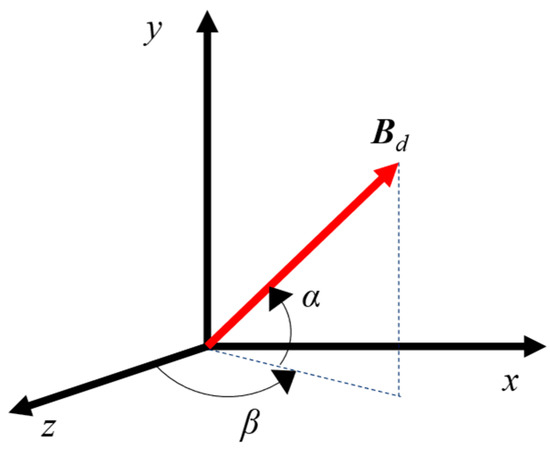
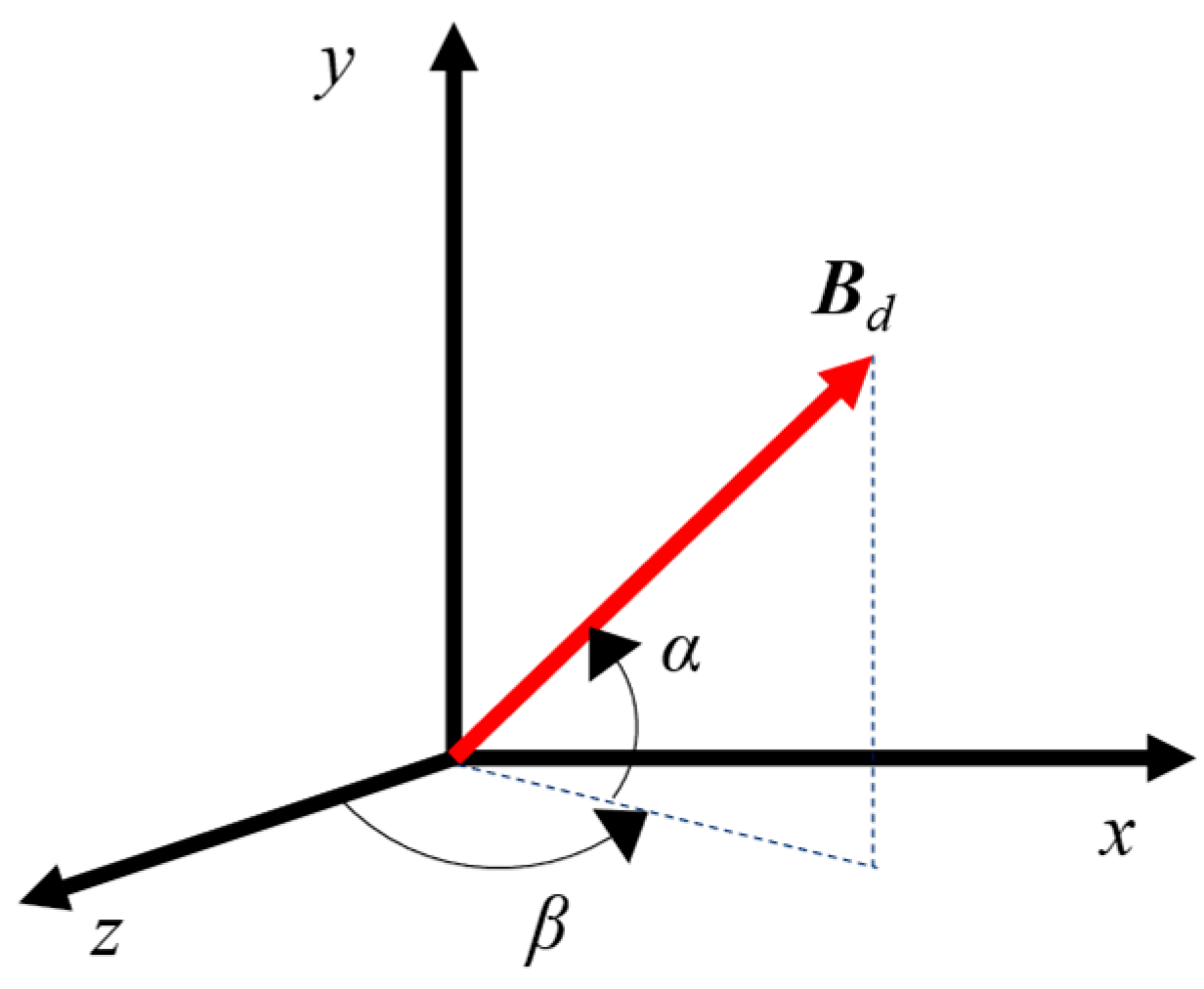
with $\alpha$ and $\beta$ defining dipole orientation in its reference frame. Figure 1 illustrates the reference coordinate system adopted for the dipole orientation angles $\alpha$ and $\beta$, as defined in reference [31]. The angle $\beta$ represents the azimuth angle in the $xy$-plane, while $\alpha$ denotes the elevation angle with respect to the $xy$-plane.

Figure 1. Reference coordinate system adopted for the dipole orientation vector ${\mathit{B}}_d$ [31].

For $P$ objects, the total field ${\mathit{B}}_d^e$ is the sum of individual dipoles:

$${\mathit{B}}_d^e={\displaystyle \sum _{p=1}^P}{\mathit{B}}_{Dp}$$

(3)

where ${\mathit{B}}_{Dp}$ is the field of the $p$-th dipole and superscript $e$ denotes a theoretical estimation.

2.2. Disturbance Estimation Concept

Object positions, obtained by exploiting a DS such as LiDAR or stereo vision, are used to estimate disturbances and the Earth’s magnetic field vector $\mathit{E}$, assuming only its magnitude $E$ is known. The measured geomagnetic magnitude is constant across space and independent of sensor orientation, while its components vary with orientation. In a disturbed location:

$$\mathit{E}={\mathit{B}}_{Sj}^m-{\mathit{B}}_{dis\_j}^r,$$

(4)

where ${\mathit{B}}_{Sj}^m$ is the measured field at sensor $j$, and ${\mathit{B}}_{dis\_j}^r$ is the real disturbance generated by all disturbing objects in the position of the sensor $j$. The superscripts $m$ and $r$ denote measured and real quantities, respectively.

An array of magnetometers allows computation of pairwise differences:

$${\mathit{d}}_i^m=\left[{\mathit{B}}_{Sj}^m-{\mathit{B}}_{Sk}^m\right],$$

(5)

where $j\ne k$, and $i$ is the sensor pair index. This cancels $\mathit{E}$, leaving only disturbance-dependent terms determined by sensor geometry. Disturbances are estimated via a dipole model evaluated at each sensor, using (1)–(4), to obtain:

$${\mathit{d}}_i^e=\left[{\mathit{B}}_{dj}^e-{\mathit{B}}_{dk}^e\right],$$

(6)

where ${\mathit{B}}_{dj}^e$ and ${\mathit{B}}_{dk}^e$ are estimated disturbances at sensors $j$ and $k$, respectively.

Parameters are found by minimizing:

$$f=f_1+f_2,$$

(7)

where:

$$f_1={\displaystyle {\sum }_{i=1}^I}\left(\left|d_{xi}^m-d_{xi}^e\right|+\left|d_{yi}^m-d_{yi}^e\right|+\left|d_{zi}^m-d_{zi}^e\right|\right),$$

(8)

matches measured and estimated differences (where $I$ is the total number of sensor pairs), and

$$f_2={\displaystyle {\sum }_{j=1}^J}\left|E^m-E_j^e\right|,$$

(9)

enforces the known magnitude $E^m=E$, where $J$ is the total number of sensors. The theoretic estimation of the Earth’s magnetic field magnitude at each sensor is defined as

$$E_j^e=‖{\mathit{E}}_j^e‖$$

(10)

where the vector term is obtained by applying:

$${\mathit{E}}_j^e={\mathit{B}}_{Sj}^m-{\mathit{B}}_{dj}^e.$$

(11)

Solving the optimization yields three parameters per object which, by adopting the vectorial form, are given as:

$${\mathit{m}}_d=B_T\widehat{\mathit{m}}={B_T\left[\left(\begin{array}{ccc}\mathit{cos}\left(\alpha \right)\mathit{cos}\left(\beta \right))& (\mathit{cos}\left(\alpha \right)\mathit{sin}\left(\beta \right))& \mathit{sin}(\alpha \end{array}\right)\right]}^T.$$

(12)

With known object positions from the DS, only these parameters are unknown. Once the optimization problem is solved, disturbances can be computed and $\mathit{E}$ estimated from (11) using data of one sensor of the array.

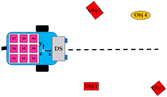
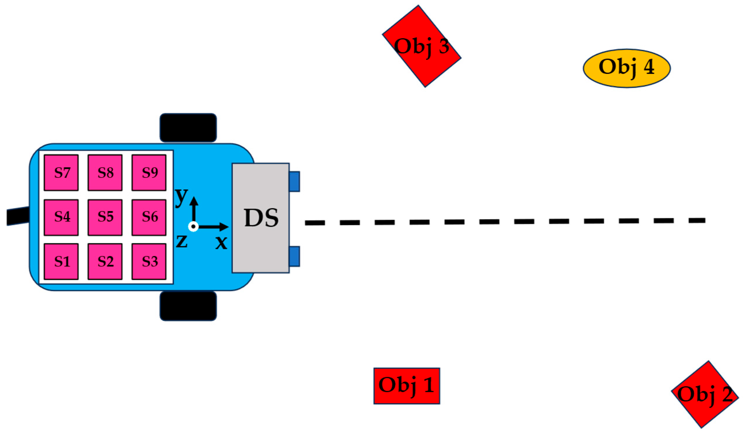
Figure 2 shows, as an example, an application where a wheeled robot, with nine magnetometers and a DS, travels through magnetic (red) and non-magnetic (yellow) objects, estimating disturbances and improving localization.

Figure 2. Example of an application: a wheeled robot is moving through disturbing (red) and non-disturbing (yellow) objects. The robot has three wheels (black): two driving wheels and a small castor wheel. The pink squares represent the magnetometers of the array, while the dashed black line indicates the robot trajectory.

2.3. Method (i) and (ii) and Their Validation

The disturbance estimation concept was validated in [28] through experimental analysis. In the theoretical analysis, arrays with varying numbers of sensors were tested against different configurations of magnetic and non-magnetic objects, each magnetic object being modeled as a dipole. The results showed that the proposed technique can accurately estimate dipole parameters when the number of objects is less than the number of sensors and remains effective even if one of the detected objects is non-magnetic.

Two formulations of the method were introduced. Method (i) employs Equations (1)–(12) as presented here, placing the equivalent dipole at the center of the volume enclosing the object. Method (ii) introduces additional degrees of freedom by allowing the dipole to move within this volume so that the optimization can determine its best position. This approach addresses the limitation of fixing the dipole at a predefined location—such as the volume center—based solely on DS information, which can be too restrictive. Allowing the dipole to move compensates for errors and accounts for the complexity of real objects, which may consist of diverse materials, shapes, and textures. The relaxation is implemented through a three-parameter shift vector, added to the DS-based position and constrained within the object’s volume. More specifically, let ${\mathbf{p}}_{DS}$ denote the object position obtained through a DS, typically corresponding to the center of the volume enclosing the object. The estimation of this position is outside the scope of the present work and is assumed to be obtained through an external detection and estimation process. In method (ii), the equivalent dipole position is corrected through a shift vector

$$\Delta \mathbf{p}=[\begin{array}{ccc}\Delta x& \Delta y& \Delta z\end{array}{]}^T$$

(13)

such that the corrected dipole position becomes

$${\mathbf{p}}_d={\mathbf{p}}_{DS}+\Delta \mathbf{p}.$$

(14)

The shift vector components are treated as additional optimization parameters and are constrained within the physical volume associated with the detected object. The corrected position ${\mathbf{p}}_d$ is then used in the computation of the vector $\mathbf{R}$ in (1), which represents the relative position between the dipole and the considered sensor. Consequently, the optimization process simultaneously estimates both the dipole moment parameters in (12) and the equivalent dipole location that best reproduces the measured magnetic disturbances.

The optimization results showed that this approach achieves better disturbance compensation. In this work, only method (ii) is investigated, using a nine-sensor array.

3. Experimental Setup

The experimental procedure described in [28] for method validation is adopted here and summarized as follows. The proposed method is evaluated using real disturbances generated by metallic objects in various scenarios. Disturbance fingerprints for each scenario are measured using the approach proposed in [32], after which the compensation method is applied in an offline phase.

3.1. Measurement of Disturbances

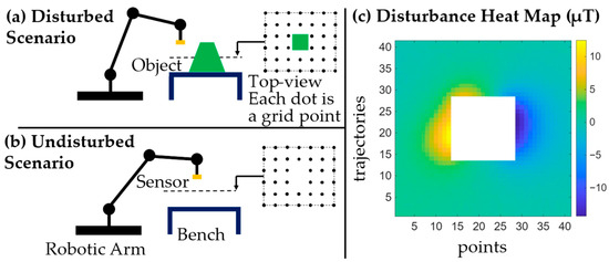
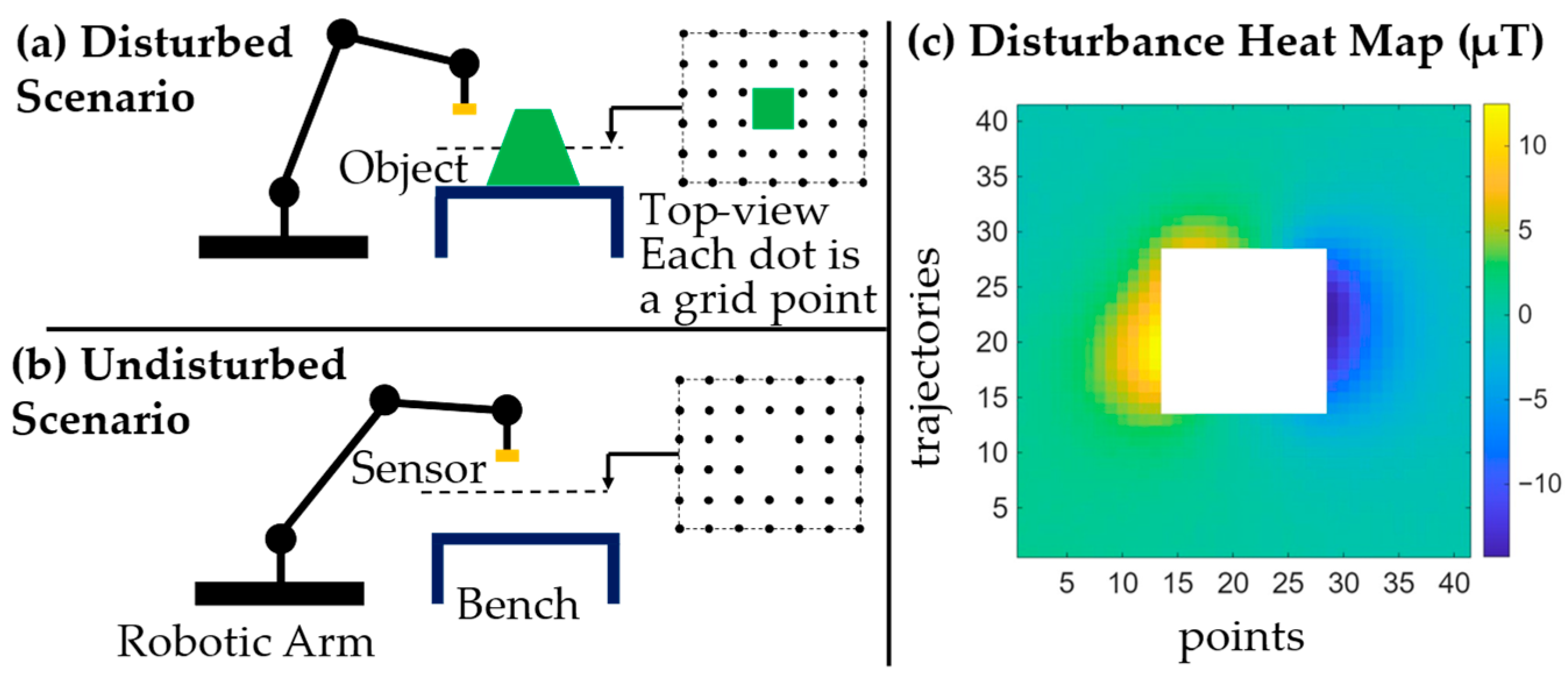
The disturbance measurement approach from [32] uses an ABB IRB140 industrial robotic arm (ABB Robotics, Zurich, Switzerland) equipped with an HMC5883L vector magnetometer (Honeywell International Inc., Charlotte, NC, USA) as the end effector to scan the magnetic field around metallic objects. Two cases are recorded: disturbed (object present) and undisturbed (object absent). Measurements are taken over a predefined grid, and the magnetic fingerprint at each point is obtained by subtracting the undisturbed measurements from the disturbed ones, allowing the removal of any external influence and leaving only the disturbance generated by the considered object. This process produces heatmaps for each disturbance magnetic component and can also be adopted for multi-object configurations. Figure 3a,b report a schematic representation of the fingerprint extraction for a generic object with a truncated pyramid shape (green). Figure 3c presents a real heatmap illustrating the magnetic disturbance produced in a given area around one of the investigated objects, which features a C-shaped geometry. The heatmap shown in Figure 3c is reported only as an illustrative example of the disturbance extraction process for one of the investigated objects and does not represent the complete set of experimental scenarios analyzed in this work. This grid-based robotic-arm method has several advantages, such as precise magnetometer alignment, uniform calibration, mitigation of static magnetic sources, controlled temperature conditions, and flexibility to test various array configurations offline.

Figure 3. (a,b) show a schematic representation of the disturbance extraction process, while (c) presents a heatmap of the disturbance obtained for a real metallic object similar to one of those investigated. The black dots represent the predefined measurement points of the grid.

3.2. Investigated Scenarios and Adopted Hardware

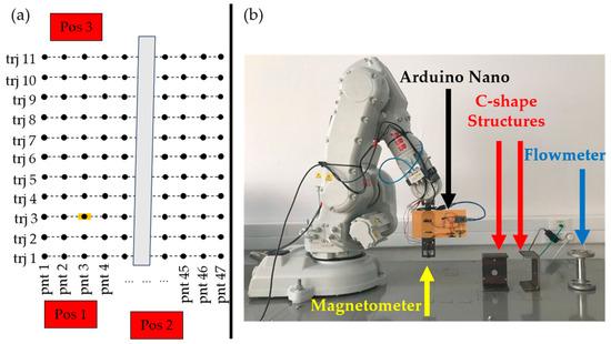
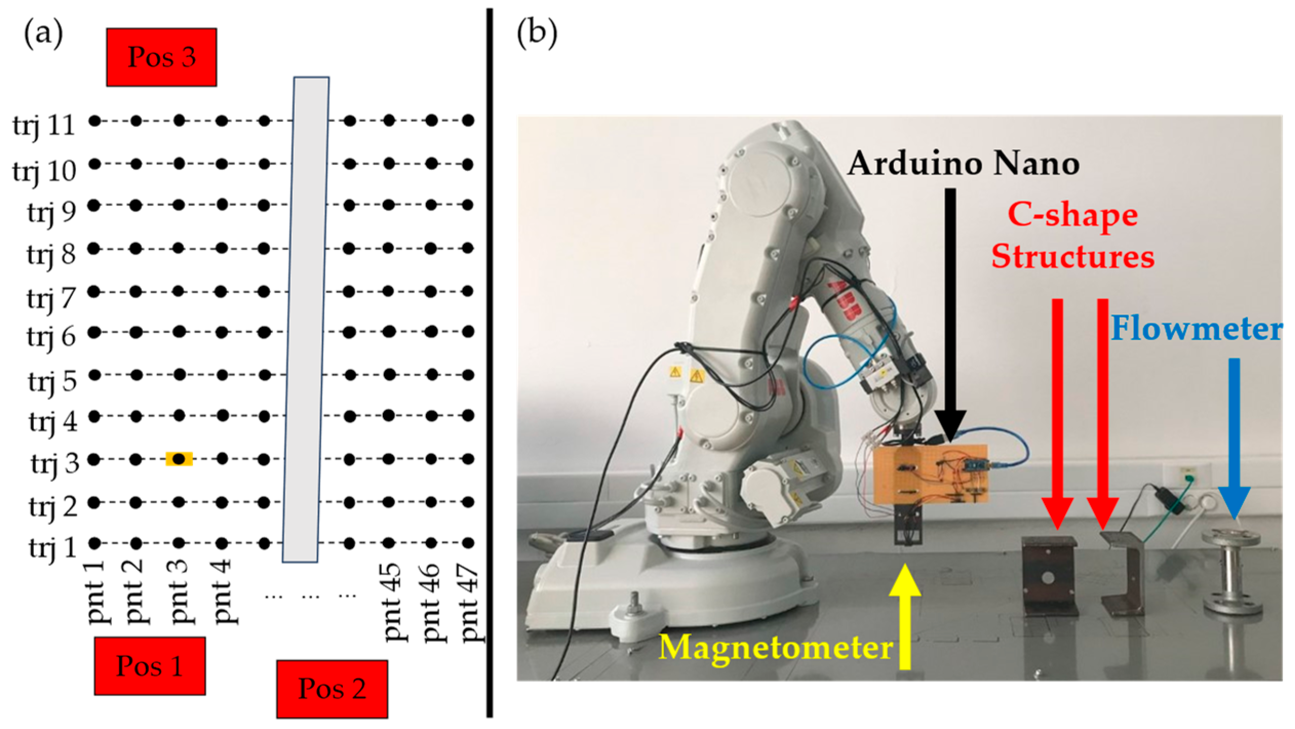
Five disturbed scenarios were measured within a 46 × 10 cm area, sampled at 1 cm intervals. Figure 4a presents a schematic representation of the measurement grid (black dots) and the magnetometer (yellow rectangle), yielding a grid composed of 11 trajectories (trjs), each consisting of 47 measurement points (pnts). Unlike Figure 3a, Figure 4a presents the specific object arrangements and measurement area adopted for the experimental evaluation.

Figure 4. (a) Layout of the investigated grid with an example arrangement of objects. The black dots represent the predefined measurement points of the grid, while the yellow symbol indicates the position of the magnetometer array at trajectory 3 and point 3. (b) The ABB robotic arm, alongside the examined objects. Subfigures adapted from [28].

In each scenario, the object arrangements consisted of various configurations of metallic and non-metallic objects, with strategic positions (Pos) to induce overlapping magnetic disturbances:

• Scenario 1: 1 metallic object at Pos 1;
• Scenario 2: 1 metallic object at Pos 1 and 1 non-metallic object at Pos 2;
• Scenario 3: 2 metallic objects at Pos 1 and Pos 2;
• Scenario 4: 2 metallic objects at Pos 1 and Pos 2, plus non-metallic object at Pos 3;
• Scenario 5: 3 metallic objects at Pos 1, Pos 2, and Pos 3 (as presented in Figure 4a) as an example).

The undisturbed case (no objects) was also recorded for subtraction. Measurements were averaged over 100 samples per point to reduce noise. Figure 4b shows the experimental setup and the investigated metallic objects, which consisted of two C-shaped structures and a flowmeter. These objects do not actively generate magnetic fields, but locally distort the Earth’s magnetic field through hard-iron and soft-iron effects, producing spatially varying magnetic disturbances that can be approximated through equivalent magnetic dipole models. The objects were positioned at predefined locations on the sides of the measurement area, identified as Pos 1–Pos 3 in Figure 4a, in order to generate different disturbance scenarios with increasing complexity. Finally, for evaluation purposes, the extracted disturbance fields were numerically combined with a reference Earth-field vector set as $\mathbf{E}=[16, 16, 43{]}^T$μT (with magnitude $E^m=48.6$ μT) in order to reconstruct magnetometer measurements affected by both the Earth’s magnetic field and magnetic disturbances. This choice represents a realistic geomagnetic field for the experimental environment and ensures repeatable comparisons across scenarios.

4. Evaluation of the Method

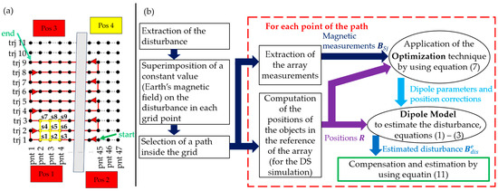
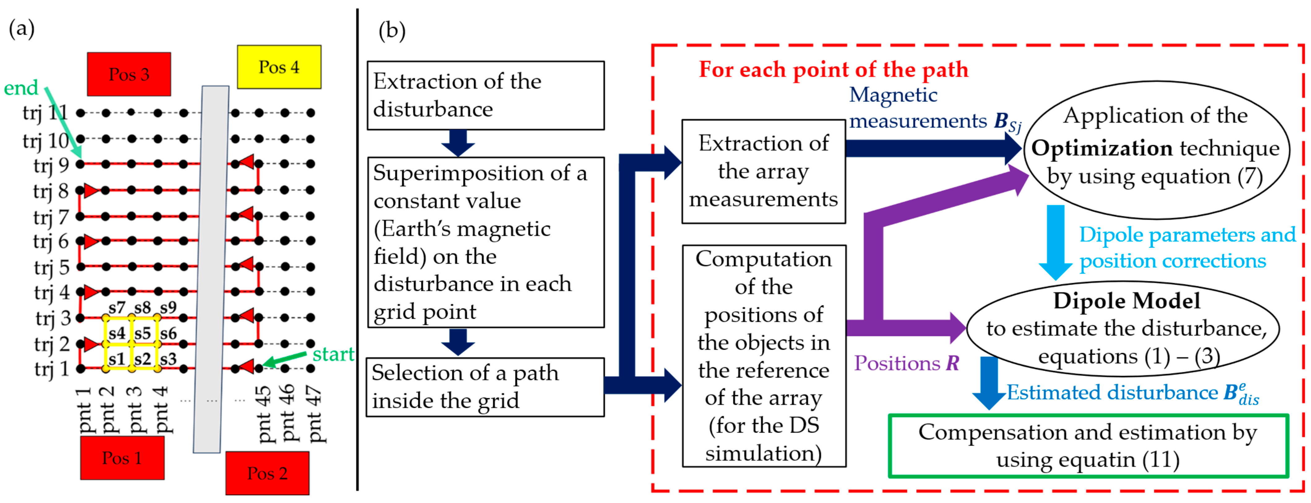
The method was implemented in MATLAB R2025b, with a custom code estimating the fitness function in (7) using a Genetic Algorithm (GA). The sensor array consists of nine magnetometers (s1–s9) arranged on a plane. The array layout is derived from the grid points shown in Figure 5a, where four adjacent 1 cm × 1 cm yellow squares define its configuration. The considered array is virtual and is reconstructed offline from the disturbance maps obtained through the robotic-arm acquisition procedure described in Section 3. More specifically, the measurements acquired by the single magnetometer mounted on the robotic arm are used to emulate the simultaneous measurements of the nine-sensor array. The array is treated as a rigid body, preserving fixed relative distances and orientations between sensors during the traversal. A path through the measured grid (red line in Figure 5a) was selected, starting at point 45 of trajectory 1 and ending at point 1 of trajectory 11. The origin and destination points are identified in the figure through green arrows and labels. The array moves along this path by following the red arrows and by preserving its heading, with magnetometer s1 serving as the reference sensor. Consequently, when s1 follows the selected path, the remaining sensors simultaneously sample neighboring grid points according to the array geometry. This configuration yields a path of 405 points with 1 cm spacing.

Figure 5. (a) Path through the grid (red line) with the array depicted by the yellow squares; the black dots represent the predefined measurement points of the grid, while the red arrows indicate the movement direction. (b) Block diagram of the evaluation process.

A block diagram, which summarizes the entire evaluation process (from extraction of the disturbance to the final estimation), is reported in Figure 5b.

As for the GA, the search bounds for the dipole parameters ${\mathbf{m}}_d$ were empirically determined through preliminary experimental evaluations to ensure stable convergence across all investigated scenarios and were set to ${\left[\pm 3.5, \pm 3.5, \pm 3.5\right]}^T$ m²A.

Further bounds are set in agreement to the volume of the identified object to allow the equivalent dipole to better locate inside the volume. It follows that, for each object (metallic or non-metallic), the number of parameters to estimate is six. The GA population size was set to 200, and the maximum number of iterations to 6000, based on empirical trials. Performance was assessed by evaluating (11) in the position of s1 and computing the MAE and Maximum Absolute Error (MaxAE) along the path, for each component $(x, y, z)$ and for the magnitude (m), comparing uncompensated and compensated magnetic fields.

Furthermore, to demonstrate that the method can be applied to a real robot localization system, the heading (or orientation) $\theta$ is evaluated. A reference frame parallel to the magnetic Earth’s reference frame is considered and it follows that the orientation can be computed as:

$$\theta =arctan\left({\displaystyle \frac{B_y}{B_x}}\right)$$

(15)

where $B_x$ and $B_y$ represent the magnetic components of the field for which angle is computed.

From (15), for each $h$-th point along the trajectory, ${\theta }^t\left(h\right)$, ${\theta }^d\left(h\right)$, and ${\theta }^e\left(h\right)$ denote the ground-truth heading (no disturbances), the heading from disturbed measurements without compensation, and the estimated heading after compensation, respectively. These quantities are used to calculate the related MAEs and MaxAE for each scenario.

5. Results and Comparison

This section presents the experimental results of the proposed method and compares them with the four-sensor configuration reported in [28]. The performance of the nine-sensor array is first analyzed through quantitative metrics and representative trends, followed by a comparative evaluation based on both absolute errors and relative improvements.

5.1. Results

All obtained errors related to each scenario for the magnetic and heading estimations are reported in Table 1. The first column reports the considered scenario that is identified by a number between 1 and 5; then, the letters N and Y identify the results obtained without and with the compensation method, respectively.

Table 1. Magnetic field and heading errors. The quantities $x, y, z$ denote the magnetic field components, while $m$ denotes the magnetic field magnitude.

Scenario	Magnetic MAE (μT)				Heading MAE (Rad)	Magnetic MaxAE (μT)				Heading MaxAE (Rad)
	x	y	z	m		x	y	z	m
1N	11.25	6.07	4.38	3.58	0.56	64.52	28.48	11.30	25.18	3.10
1Y	1.61	1.13	0.58	0.15	0.08	28.94	8.09	4.06	1.89	1.44
2N	11.25	6.07	4.38	3.58	0.56	64.52	28.48	11.30	25.18	3.10
2Y	2.38	2.63	0.98	0.14	0.14	14.58	11.89	4.54	1.28	0.71
3N	11.87	7.89	7.53	9.60	0.53	57.63	24.18	14.46	28.75	3.11
3Y	5.29	4.62	2.22	0.26	0.25	20.55	15.62	8.35	2.71	1.47
4N	11.87	7.89	7.53	9.60	0.53	57.63	24.18	14.46	28.75	3.11
4Y	6.64	5.97	2.57	0.21	0.31	32.22	29.19	18.23	3.04	3.11
5N	11.27	7.87	7.55	9.57	0.52	57.65	24.33	14.37	28.46	3.11
5Y	10.02	6.99	2.88	0.27	0.70	40.37	30.44	11.61	2.00	2.95

By analyzing Table 1, the following observations can be drawn:

• Without compensation, the magnetic field MAEs remain high across all scenarios (approximately 4–12 μT), with heading errors around 0.5 rad, confirming the strong impact of magnetic disturbances.
• The proposed compensation method significantly reduces both magnetic field and heading errors in most scenarios, with MAEs typically below 6.64 μT and heading errors below 0.31 rad.
• In low-to-moderate disturbance scenarios (1–3), substantial improvements are observed, demonstrating the effectiveness of the dipole-based model under relatively simple conditions.
• In more complex scenarios (4–5), the performance degrades, particularly in scenario 5, where the heading error increases, indicating limitations of the dipole model in the presence of multiple overlapping disturbances.
• Overall, the results show that the method effectively mitigates disturbances in simple configurations, while its accuracy decreases as the complexity of the disturbance increases.

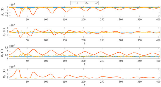
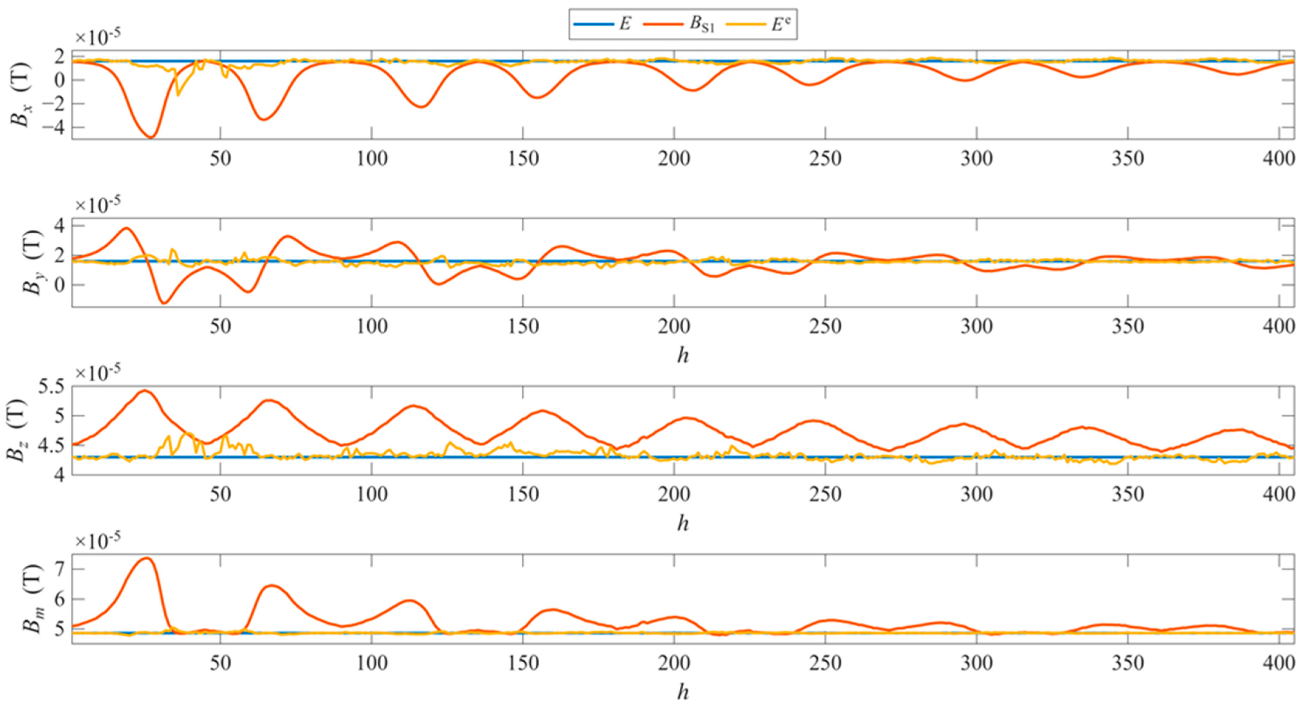
To complement the quantitative results, the magnetic field and heading trends are reported for scenario 1, which represents the most favorable case. Figure 6 shows the magnetic field trends for sensor s1 (red), the Earth’s magnetic field (blue), and the estimated geomagnetic field (yellow), plotted as a function of the trajectory points $h$.

Figure 6. Representation of magnetic field trends as functions of points h in scenario 1: the red line represents the measurement from sensor s1, the blue line corresponds to the Earth’s magnetic field, and the yellow line illustrates the estimation of the geomagnetic field.

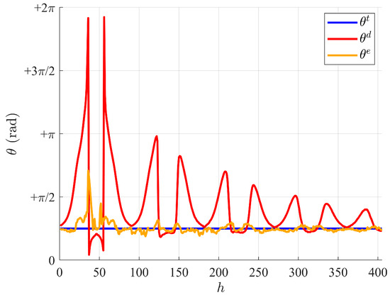
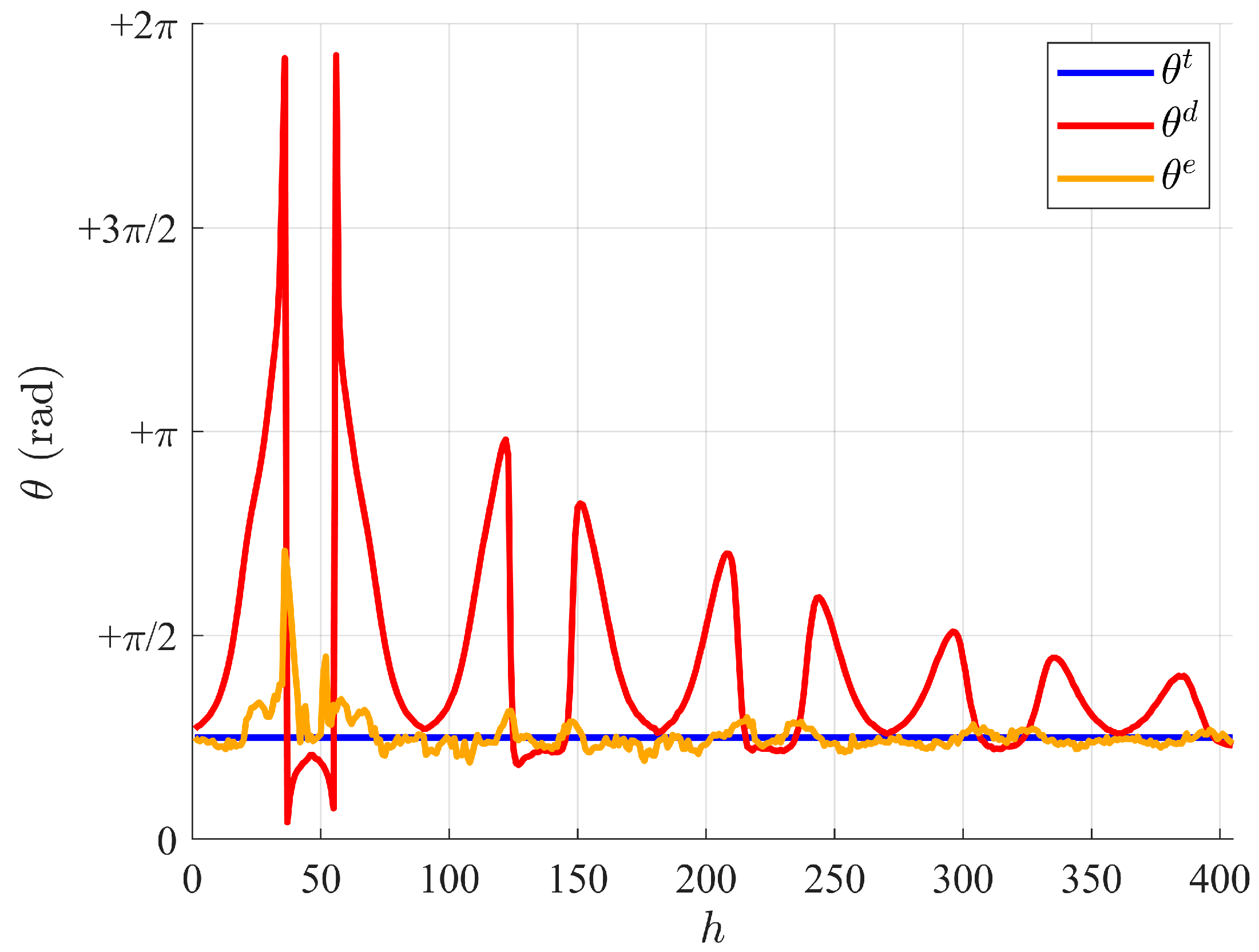
Figure 7 presents heading estimates (in the range [0, 2π]) at sensor s1 for the real (blue), disturbed (red), and compensated (yellow) geomagnetic field.

Figure 7. Heading trend of the scenario 1.

In general, both Figure 6 and Figure 7 show results with larger errors in the initial portion of the trajectory, when the array is closer to the object, with accuracy improving in the later segment. This behavior suggests that the object’s magnetic signature deviates from that of an ideal dipole.

5.2. Comparison

The results obtained in this work are consistent with those reported in [28] for method (ii). In the previous study, an array of four magnetometers and a simplified reference Earth’s magnetic field of ${\left[6.5, 6.5, 25\right]}^T$μT were considered, whereas the present work employed a larger array with nine sensors and a more realistic geomagnetic field configuration given by ${\left[16, 16, 43\right]}^T$μT. Furthermore, in the current work, the increased number of sensors resulted in a shorter trajectory length ($h=405$ points) compared to the $h=450$ points in [28], making a direct numerical comparison difficult. Therefore, a direct comparison between the two works cannot be executed straightforward. The most rigorous comparison would require repeating the four-sensor configuration under the same experimental conditions and reference the Earth-field adopted in the present work. However, the four-sensor results originate from a previous experimental measurement campaign and subsequent offline evaluation, and therefore the two datasets could not be fully harmonized retrospectively. For this reason, the comparison presented in this section is intended primarily to evaluate relative performance trends and compensation behavior rather than strict numerical superiority between the two configurations. To enable a more consistent comparison, the results reported in [28] were reprocessed by extracting only the subset of trajectory points corresponding to the path considered in the present study. This operation is justified by the fact that each grid point is evaluated independently within the adopted framework, and therefore the removal of points does not affect the estimation process at the remaining locations. Based on this reduced dataset, the MAE and MaxAE metrics were recomputed, and the corresponding results are reported in Table 2.

Table 2. Magnetic field and heading errors for the four-sensor array configuration, based on the data reported in [28], and recomputed over the trajectory of 405 points considered in this work. The quantities $x, y, z$ denote the magnetic field components, while $m$ denotes the magnetic field magnitude.

Scenario	Magnetic MAE (μT)				Heading MAE (Rad)	Magnetic MaxAE (μT)				Heading MaxAE (Rad)
	x	y	z	m		x	y	z	m
1N	11.26	6.07	4.38	6.45	1.18	64.52	28.48	11.30	41.57	3.12
1Y	1.60	1.87	0.41	0.11	0.26	18.20	13.17	1.76	0.68	1.97
2N	11.26	6.07	4.38	6.45	1.18	64.52	28.48	11.30	41.57	3.12
2Y	2.84	3.28	0.81	0.07	0.49	12.88	16.65	4.07	0.57	3.01
3N	12.64	8.14	7.50	12.11	0.90	57.63	24.81	14.46	41.35	3.12
3Y	5.34	3.30	1.11	0.08	0.78	26.73	11.51	9.83	1.10	3.01
4N	12.64	8.14	7.50	12.11	0.90	57.63	24.81	14.46	41.35	3.12
4Y	5.14	3.77	1.15	0.06	0.81	13.43	13.03	4.83	0.46	3.04
5N	12.04	8.12	7.53	12.01	0.88	57.65	25.32	14.37	40.88	3.12
5Y	5.72	4.71	1.30	0.07	1.04	15.93	17.84	4.80	0.49	3.13

It is noted, however, that a complete alignment between the two studies cannot be achieved, as the reference Earth’s magnetic field differs between the experiments.

This aspect cannot be compensated for retrospectively and, due to the nonlinear relationship between magnetic components and heading estimation, it may influence the resulting heading errors. Consequently, the comparison should not be interpreted as a fully controlled direct experimental validation between the four-sensor and nine-sensor configurations. Instead, the analysis is intended to highlight relative trends in compensation performance and robustness across the investigated scenarios.

Additionally, the MAE values reported in Table 2 are slightly higher than those originally presented in [28]. This difference is attributed to the reduced trajectory length adopted in the present analysis, as the MAE is computed as an average over the considered points and is therefore sensitive to the number and distribution of samples. In contrast, the MaxAE values remain unchanged, since they depend only on the maximum deviation and are not affected by the number of trajectory points.

By analyzing Table 2, similar trends to those observed in Table 1 can be identified. In particular, the compensation method provides a noticeable reduction in magnetic and heading errors in low-to-moderate disturbance scenarios (scenarios 1–3), while its effectiveness decreases in more complex configurations (scenarios 4–5). In scenario 5, the compensation leads to an increase in heading MAE, confirming the limitations of the dipole-based model under strong and overlapping disturbances. Overall, the four-sensor configuration exhibits qualitatively consistent behavior with the nine-sensor case, although with reduced effectiveness. These results indicate that the present work not only implements a larger array, but also evaluates how increasing the number of magnetometers affects the compensation behavior, the robustness of heading estimation, and the limitations of the equivalent-dipole formulation under more complex disturbance conditions.

To better highlight the impact of the increased number of sensors, the relative improvements in the heading error metrics are evaluated for both array configurations. The percentage improvement of the considered metrics (MAE and MaxAE) is defined as:

$$I=\frac{E_N-E_Y}{E_N} \times 100$$

(16)

where $E_N$ and $E_Y$ denote the value of the considered error metric (either MAE or MaxAE) in the uncompensated and compensated cases, respectively. By applying (16) to the results reported in Table 1 and Table 2, the corresponding percentage improvements are obtained and summarized in Table 3.

Table 3. Percentage improvement in heading error metrics (MAE and MaxAE) for the nine-sensor and four-sensor array [28] configurations across all scenarios.

Scenario	Nine-Sensor Array		Four-Sensor Array
	${\mathit{I}}_{\mathit{M}\mathit{A}\mathit{E}}$ %	${\mathit{I}}_{\mathit{M}\mathit{a}\mathit{x}\mathit{A}\mathit{E}}$ %	${\mathit{I}}_{\mathit{M}\mathit{A}\mathit{E}}$ %	${\mathit{I}}_{\mathit{M}\mathit{a}\mathit{x}\mathit{A}\mathit{E}}$ %
1	85.71	53.55	77.97	36.86
2	75.00	77.10	58.47	3.53
3	52.83	52.73	13.33	3.53
4	41.51	0.00	10.00	2.56
5	−34.62	5.14	−18.18	−0.32

The percentage improvements reported in Table 3 enable a more direct comparison of the compensation performance for the two-sensor array configurations. It is noted, however, that the heading is computed from magnetic components through a nonlinear arctangent relationship, and therefore the percentage reduction in heading error is not strictly invariant to changes in the underlying magnetic field magnitude and direction. Nevertheless, this metric provides a meaningful indication of the relative effectiveness of the compensation method within each scenario and allows a more consistent comparison between configurations.

In low-to-moderate disturbance scenarios (scenarios 1–3), the nine-sensor array consistently achieves higher improvements in heading MAE compared to the four-sensor configuration. In particular, a substantial gain is observed in scenario 3, where the improvement increases from approximately 13% to over 50%, highlighting the benefit of a higher number of sensors in more complex disturbance conditions.

In scenario 4, both configurations exhibit reduced effectiveness, although the nine-sensor array still maintains a higher improvement (approximately 41%) compared to the four-sensor case (approximately 10%). This indicates that increasing the number of sensors enhances robustness, even when the disturbance configuration becomes more challenging.

In scenario 5, both configurations show negative improvement values, indicating a degradation of performance. This confirms that, under strong and overlapping disturbances, the dipole-based model is no longer sufficient to accurately represent the magnetic field. Notably, the degradation is more pronounced for the nine-sensor array, suggesting that increasing the number of sensors alone is not sufficient to overcome model limitations in highly complex scenarios. This observation is consistent with the indications in [28], where it was highlighted that improved performance requires not only a higher number of sensors but also a compact array configuration with reduced spatial extent. In the present setup, such a reduced array surface was not implemented, which may have limited the achievable performance in highly disturbed conditions.

A similar trend can be observed for the MaxAE metric. The nine-sensor configuration generally provides significantly higher reductions in worst-case errors, whereas the four-sensor array shows limited or negligible improvement in several scenarios.

Overall, these results demonstrate that increasing the number of sensors leads to a clear enhancement in compensation performance in most scenarios, particularly in terms of average error reduction, while also highlighting the limitations of the adopted model in highly disturbed environments.

A fully controlled comparative validation between the two array configurations under identical magnetic field conditions is identified as an important direction for future work.

6. Conclusions

This paper proposed and experimentally validated an enhanced dipole model-based method for compensating magnetic disturbances using a magnetometer array with increased sensor density. The results indicate that the proposed nine-sensor configuration improves compensation performance in most investigated scenarios and exhibits more favorable relative error-reduction trends than the lower-density configuration considered for comparison.

In particular, magnetic field errors were reduced to below 6.64 µT and heading errors to 0.31 rad in most scenarios, with improvements exceeding 50% and reaching values as low as 0.15 μT and 0.08 rad in the best case.

The analysis further showed that increasing sensor density leads to consistent improvements in both MAEs and MaxAEs, confirming the scalability of the dipole-based approach. However, in highly complex disturbance scenarios, performance degradation was observed, highlighting the limitations of modeling real-world objects as ideal dipoles. Nevertheless, because the four-sensor and nine-sensor datasets were obtained under different reference Earth-field conditions, the comparison should be interpreted as a trend-based assessment rather than as a fully controlled direct experimental comparison.

These findings indicate that magnetometer arrays with higher sensor density represent an effective solution for improving disturbance compensation performance. At the same time, the results suggest that further enhancements may be achieved by adopting more compact array geometries and exploring multi-layer configurations. Overall, the proposed approach provides a practical framework for improving the robustness of magnetometer-based localization systems operating in magnetically disturbed environments.

References

- Lv, W.; Kang, Y.; Qin, J. Indoor Localization for Skid-Steering Mobile Robot by Fusing Encoder, Gyroscope, and Magnetometer. IEEE Trans. Syst. Man Cybern. Syst. 2019, 49, 1241–1253. [Google Scholar] [CrossRef] [Scilit]
- Jung, J.; Lee, S.M.; Myung, H. Indoor Mobile Robot Localization and Mapping Based on Ambient Magnetic Fields and Aiding Radio Sources. IEEE Trans. Instrum. Meas. 2015, 64, 1922–1934. [Google Scholar] [CrossRef] [Scilit]
- Štancel, M.; Hurtuk, J.; Hulič, M.; Červeňák, J. Indoor Atlas Service as a Tool for Building an Interior Navigation System. Acta Polytech. Hung. 2021, 18, 87–110. [Google Scholar] [CrossRef] [Scilit]
- Shao, W.; Zhao, F.; Wang, C.; Luo, H.; Muhammad Zahid, T.; Wang, Q.; Li, D. Location Fingerprint Extraction for Magnetic Field Magnitude Based Indoor Positioning. J. Sens. 2016, 2016, 1945695. [Google Scholar] [CrossRef] [Scilit]
- Hostettler, R.; Djurić, P.M. Vehicle Tracking Based on Fusion of Magnetometer and Accelerometer Sensor Measurements With Particle Filtering. IEEE Trans. Veh. Technol. 2015, 64, 4917–4928. [Google Scholar] [CrossRef] [Scilit]
- Wahlström, N.; Gustafsson, F. Magnetometer Modeling and Validation for Tracking Metallic Targets. IEEE Trans. Signal Process. 2014, 62, 545–556. [Google Scholar] [CrossRef] [Scilit]
- Ma, W.; Xing, D.; McKee, A.; Bajwa, R.; Flores, C.; Fuller, B.; Varaiya, P. A Wireless Accelerometer-Based Automatic Vehicle Classification Prototype System. IEEE Trans. Intell. Transp. Syst. 2014, 15, 104–111. [Google Scholar] [CrossRef] [Scilit]
- Cheung, S.Y.; Coleri, S.; Dundar, B.; Ganesh, S.; Tan, C.W.; Varaiya, P. Traffic Measurement and Vehicle Classification with Single Magnetic Sensor. In Proceedings of the Transportation Research Record; SAGE Publishing: Thousand Oaks, CA, USA, 2005. [Google Scholar]
- Pizzocaro, S.; Corno, M.; Pantano, M.; Savaresi, S. Magnetometer Aided GPS-Free Localization of an Autonomous Vineyard Drone. In Proceedings of the 2021 European Control Conference, ECC 2021, Rotterdam, The Netherlands, 29 June–2 July 2021. [Google Scholar]
- Wang, Y.; Fu, Q.; Sui, Y. A Robust Tracking Method for Multiple Moving Targets Based on Equivalent Magnetic Force. Micromachines 2022, 13, 2018. [Google Scholar] [CrossRef] [Scilit]
- Fan, L.; Kang, C.; Zhang, X.; Zheng, Q.; Wang, M. An Efficient Method for Tracking a Magnetic Target Using Scalar Magnetometer Array. Springerplus 2016, 5, 502. [Google Scholar] [CrossRef] [Scilit]
- Lv, B.; Qin, Y.; Dai, H.; Su, S. Improving Localization Success Rate of Three Magnetic Targets Using Individual Memory-Based WO-LM Algorithm. IEEE Sens. J. 2021, 21, 21750–21758. [Google Scholar] [CrossRef] [Scilit]
- Skog, I.; Kok, M.; Hendeby, G.; Huang, C.; Edridge, T. On the Connection Between Magnetic-Field Odometry Aided Inertial Navigation and Magnetic-Field SLAM. In Proceedings of the 2025 IEEE/ION Position, Location and Navigation Symposium, PLANS 2025, Salt Lake City, UT, USA, 28 April–1 May 2025. [Google Scholar]
- Kok, M.; Solin, A. Scalable Magnetic Field SLAM in 3D Using Gaussian Process Maps. In Proceedings of the 2018 21st International Conference on Information Fusion, FUSION 2018, Cambridge, UK, 10–13 July 2018. [Google Scholar]
- Hadjigeorgiou, N.; Asimakopoulos, K.; Papafotis, K.; Sotiriadis, P.P. Vector Magnetic Field Sensors: Operating Principles, Calibration, and Applications. IEEE Sens. J. 2021, 21, 12531–12544. [Google Scholar] [CrossRef] [Scilit]
- Yousefi, M.; Nejat Pishkenari, H.; Alasty, A. A Fast and Robust Magnetic Localization Technique Based on Elimination of the Orientation Variables from the Optimization. IEEE Sens. J. 2021, 21, 21885–21892. [Google Scholar] [CrossRef] [Scilit]
- Yi, J.; Liu, J.; Zhang, C.; Lu, X. Magnetic Motion Tracking for Natural Human Computer Interaction: A Review. IEEE Sens. J. 2022, 22, 22356–22367. [Google Scholar] [CrossRef] [Scilit]
- Wang, M.; Shi, Q.; Song, S.; Hu, C.; Meng, M.Q.H. A Novel Relative Position Estimation Method for Capsule Robot Moving in Gastrointestinal Tract. Sensors 2019, 19, 2746. [Google Scholar] [CrossRef] [Scilit]
- Yin, G.; Zhang, L.; Jiang, H.; Wei, Z.; Xie, Y. A Closed-Form Formula for Magnetic Dipole Localization by Measurement of Its Magnetic Field Vector and Magnetic Gradient Tensor. J. Magn. Magn. Mater. 2020, 499, 166274. [Google Scholar] [CrossRef] [Scilit]
- Stefanoni, M.; Odry, Á.; Sarcevic, P. A Closed-Form Formula-Based Method for Magnetic Dipole Localization in a Constant Magnetic Field by Measurement of Its Magnetic Field Vectors and Magnetic Gradient Tensors. J. Magn. Magn. Mater. 2025, 629, 173313. [Google Scholar] [CrossRef] [Scilit]
- Liu, G.; Zhang, Y.; Wang, C.; Li, Q.; Li, F.; Liu, W. A New Magnetic Target Localization Method Based on Two-Point Magnetic Gradient Tensor. Remote Sens. 2022, 14, 6088. [Google Scholar] [CrossRef] [Scilit]
- You, H.; Li, J.; Xu, J.; Xu, J.; Ning, T.; Gao, Y.; Li, L. A Method for Estimating Magnetic Target Location by Employing Total Field and Its Gradients Data. Sci. Rep. 2022, 12, 17985. [Google Scholar] [CrossRef] [Scilit]
- Wang, M.; Lin, J.; Wang, Y.; Zhao, J. Multiobject Localization Using Magnetic Tensor Gradiometer Array and Improved IForest. IEEE Geosci. Remote Sens. Lett. 2022, 19, 8023405. [Google Scholar] [CrossRef] [Scilit]
- Li, Q.; Li, Z.; Shi, Z.; Fan, H. Multi-Target Magnetic Positioning Using SAFCM Clustering and Invariants-Improved Tilt Angle. IEEE Trans. Geosci. Remote Sens. 2022, 60, 5924015. [Google Scholar] [CrossRef] [Scilit]
- Secer, G.; Barshan, B. Improvements in Deterministic Error Modeling and Calibration of Inertial Sensors and Magnetometers. Sens. Actuators A Phys. 2016, 247, 522–538. [Google Scholar] [CrossRef] [Scilit]
- Wu, Y.; Shi, W. On Calibration of Three-Axis Magnetometer. IEEE Sens. J. 2015, 15, 6424–6431. [Google Scholar] [CrossRef] [Scilit]
- Kok, M.; Schon, T.B. Magnetometer Calibration Using Inertial Sensors. IEEE Sens. J. 2016, 16, 5679–5689. [Google Scholar] [CrossRef] [Scilit]
- Stefanoni, M.; Odry, A.; Sarcevic, P. Dipole Model-Based Disturbance Compensation Using Magnetometer Arrays. IEEE Trans. Instrum. Meas. 2025, 74, 9515110. [Google Scholar] [CrossRef] [Scilit]
- Stefanoni, M.; Odry, A.; Sarcevic, P. A Neural Network-Based Approach for the Identification and Compensation of Magnetic Disturbances in Mobile Robot Localization. In Proceedings of the SACI 2023—IEEE 17th International Symposium on Applied Computational Intelligence and Informatics, Timișoara, Romania, 23–26 May 2023. [Google Scholar]
- Stefanoni, M.; Odry, A.; Sarcevic, P. A Dipole Model-Based Approach for Magnetic Disturbance Compensation of Mobile Robots Using Magnetometer Arrays. In Proceedings of the IEEE 23rd International Symposium on Computational Intelligence and Informatics, CINTI 2023, Budapest, Hungary, 20–22 November 2023. [Google Scholar]
- Stefanoni, M.; Odry, A.; Sarcevic, P. Dipole Model-Based Magnetic Disturbance Compensation Method for Mobile Robots Using a Magnetometer Array. In Proceedings of the 2024 IEEE Sensors Applications Symposium (SAS), Naples, Italy, 23–25 July 2024; IEEE: Piscataway, NJ, USA, 2024; pp. 1–5. [Google Scholar]
- Stefanoni, M.; Pesti, R.; Odry, A.; Sarcevic, P. Measurement System for the Simulation of Indoor Magnetic Disturbances Using a Robotic Arm. In Proceedings of the 2023 IEEE 21st World Symposium on Applied Machine Intelligence and Informatics, SAMI 2023, Herľany, Slovakia, 19–21 January 2023. [Google Scholar]
Disclaimer/Publisher’s Note: The statements, opinions and data contained in all publications are solely those of the individual author(s) and contributor(s) and not of MDPI and/or the editor(s). MDPI and/or the editor(s) disclaim responsibility for any injury to people or property resulting from any ideas, methods, instructions or products referred to in the content. |
© 2026 by the authors. Licensee MDPI, Basel, Switzerland. This article is an open access article distributed under the terms and conditions of the Creative Commons Attribution (CC BY) license.