


Abstract
With the continuous advancement of industrial intelligence, the application of hydraulic robots is becoming increasingly widespread, and the demand for their health diagnosis and maintenance is becoming more urgent. By integrating digital twin (DT) and deep learning technologies, this paper presents an intelligent fault diagnosis method for hydraulic robots based on multi-source information fusion. Firstly, a fault diagnosis architecture and solution for hydraulic robots based on DT technology are proposed. Secondly, a DT model of the hydraulic robot, which incorporates a 3D model and an attribute model with virtual–physical synchronization capabilities, is established, and a calibration method for the twin model is explored. Next, for four typical faults—leakage in the hydraulic system, valve sticking, damping hole blockage, and filter blockage—fault mechanism analysis and evolution process simulation are conducted on the established DT model. A multi-source high-quality dataset, covering normal operating conditions and multiple fault scenarios, is constructed to drive the data twin model. Finally, a feature extraction method combining Convolutional Neural Network (CNN), Bidirectional Long Short-Term Memory (BiLSTM), and Attention mechanisms is proposed. This is followed by using a Random Forest (RF) classifier to achieve accurate fault diagnosis for various hydraulic system failures. The experimental results validate the effectiveness and practicality of this method.
1. Introduction
With the continuous advancement of intelligent manufacturing, hydraulic robots are increasingly applied in industrial manufacturing and aerospace due to their high power density, load capacity, fast dynamic response, and adaptability [1]. However, hydraulic robots typically operate in complex environments, facing continuous load fluctuations and external disturbances, leading to accelerated component wear, performance degradation, and actuator failures. Particularly in some high-precision tasks, hydraulic robots generally exhibit lower positioning accuracy compared to electric robots, limiting their application in precision operations [2]. As hydraulic robots evolve toward lightweight, miniaturized, high-pressure, and high-power configurations, their structures become more complex, imposing higher demands for safety, stability, and intelligent operation and maintenance [3]. Hydraulic robots, as a fluid–mechanical–electrical coupled system, exhibit high randomness and concealment in fault evolution, making fault diagnosis particularly challenging [4]. Thus, improving hydraulic robots’ operational stability and fault diagnosis accuracy is critical to ensuring reliable system performance.
For hydraulic robot fault diagnosis, traditional methods, exemplified by the Fourier transform, wavelet analysis, and empirical mode decomposition, mainly rely on sensor monitoring and signal processing, to extract features from pressure, flow, and vibration signals [5,6,7]. Additionally, the physical and chemical properties of oil contamination and particle size can be analyzed to assess system health [8]. Despite validated performance, there are still significant limitations associated with these methods. That is, they depend heavily on expert-designed features and exhibit limited adaptability in nonlinear, time-varying, or noisy conditions, highlighting the need for data-driven intelligent diagnosis methods.
Recently, the achievements in artificial intelligence have led to increased attention on data-driven techniques for the hydraulic robot fault diagnosis. Models such as the Convolutional Neural Networks (CNN), Recurrent Neural Networks (RNN), and Long Short-Term Memory Networks (LSTM) are applied to automated feature extraction and fault pattern recognition for hydraulic robot fault diagnosis [9]. For instance, Peng and Wang [10] proposed a multi-condition fault diagnosis method for diagnosing the faults of Rotary Vectorreducers (RV) based on a deep CNN with robustness against noise; Jiang et al. [11] addressed low diagnostic accuracy in traditional machine learning by proposing an XGBoost-based implicit feature extraction and SVM-based multi-fault mode recognition method. Tang et al. [12] introduced a CNN-BO method integrating Bayesian optimization with the CNN, significantly enhancing the diagnostic accuracy and robustness for multiple fault types of hydraulic piston pumps. Sun et al. [13] developed an intelligent fault diagnosis method using a multi-scale 1D CNN, improving the fault recognition capability in hydraulic systems. Although these methods progress in feature extraction and pattern recognition, they require large, high-quality labeled datasets, which are often scarce in practice [14].
The enhancement of hydraulic robot safety and stability, along with accurate fault diagnosis, constitutes a complex engineering task. Progress in this area relies on the integration of mechanical control, fluid power, intelligent algorithms, and state monitoring technologies while balancing efficiency and cost [15]. In this context, the digital twin (DT) technology offers a novel approach for fault diagnosis in hydraulic robots, owing to outstanding advantages. The DT creates a high-fidelity virtual model that is aligned with the physical system, integrating real-time sensor data and historical data for bidirectional mapping and dynamic interaction between the physical entity and the virtual model. This improves the integrated management and control capabilities of the system [16]. In the context of Industry 5.0, digital twin technology not only helps optimize production efficiency but also plays a central role in enhancing resource utilization, improving energy efficiency, and driving the realization of sustainable manufacturing. Industry 5.0 emphasizes human–machine collaboration and flexible, customized production, where digital twin technology serves as a crucial tool to achieve these goals. By enabling real-time monitoring and interaction between the physical system and virtual models, digital twin technology facilitates a more efficient and adaptive manufacturing process that aligns with the principles of Industry 5.0. It supports not only the automation of fault diagnosis but also helps optimize production processes, thus contributing to a more sustainable and efficient industrial environment [2,17].
DT technology enables real-time perception and analysis of a hydraulic robot’s operating state. Faults manifest as changes in motion performance and working conditions, leading to observable fluctuations in key physical parameters—such as pressure, flow, and displacement—across the hydraulic system and its actuators. By leveraging DT to monitor these signals and perform virtual–physical comparisons in real time, the framework provides a data-driven basis for rapid fault identification and precise localization.
Compared to traditional fault diagnosis methods for hydraulic robots, the DT enables real-time equipment status monitoring and simulates typical fault scenarios in a virtual environment, generating diverse high-quality fault datasets to address the shortage of actual fault data [18]. The DT can also identify discrepancies between physical and virtual systems. By compensating with data and optimizing the model, simulation accuracy is improved, enhancing prediction and diagnostic capabilities under complex operating conditions. Existing studies demonstrate that DT-based intelligent diagnostic frameworks can enhance diagnostic performance despite model uncertainties and challenges in obtaining fault data [19]. For example, Liu and David [20] proposed an AI simulation framework based on DT to address data scarcity, and Li et al. [21] developed an intelligent fault diagnosis method for centrifugal pump impeller mechanical faults using DT flow field cloud maps and the Yolov5 algorithm.
In recent years, significant progress has been made in DT modeling and intelligent fault diagnosis for hydraulic robotic systems. Zhang et al. [22] developed a DT framework for industrial parallel robots and established a spatial kinematic model to support twin–physical synchronization. By introducing an Improved Particle Swarm Optimization–Sparrow Search Algorithm–Deep Backpropagation Network (IPSO-SSA-DBP) algorithm, they achieved calibration of kinematic parameters and prediction of pose errors. Based on this, a digital twin-based system integrating status monitoring and positioning error compensation was constructed. Jian et al. [23] proposed a DT-based hydraulic circuit simulation system that utilizes precise virtual modeling and real-time data synchronization for data collection, storage, and visualization. Liang et al. [24] presented a hybrid DT approach that combines physical with data-driven models to create a high-fidelity twin of an electro-hydraulic servo valve. This method generates fault data for training a CNN model, improving the diagnostic accuracy under limited fault samples. Sun et al. [25] introduced a DT-based hydraulic system fault diagnosis method to address model parameter uncertainty and low diagnostic accuracy. Wang et al. [4] proposed a DT framework combining virtual models and physical entities to resolve hydraulic system faults, providing a viable solution for fault diagnosis.
Despite the above progress in the DT technology for fault diagnosis for hydraulic robotic systems, significant shortcomings persist. Firstly, the existing methods rely on large, high-quality labeled datasets, whereas real fault data in engineering settings are scarce, resulting in inadequate model training. Secondly, many of these approaches have poor generalization beyond single operating conditions or a limited range of faults, lacking adaptability in multi-condition and multi-fault scenarios. Thirdly, the temporal dependencies and heterogeneous signal fusion are inadequately modeled, which compromises the stability and robustness of the DT model.
To address these limitations of the existing fault diagnosis methods for hydraulic robots in complex operating conditions, this paper develops a novel DT-based fault diagnosis framework that integrates both physical model and data-driven models with multi-source information fusion. Our main contributions are summarized as follows.
- A DT-Based intelligent fault diagnosis architecture consisting of five layers is designed for the hydraulic robotic system;
- A DT model of the hydraulic robot with accurate state perception, virtual–physical synchronization, and continuous online calibration is established, enabling high-fidelity simulation and dynamic and consistent behavior modeling under various fault conditions;
- A high-quality multi-source dataset covering multiple operating conditions and multiple fault categories is constructed for diagnostic generalization and reliability improvement, without the costs and risks of destructive testing;
- An end-to-end diagnosis pipeline, named CNN-BiLSTM-Attention-RF (CBAR), is proposed by leveraging advantages of various deep learning models for automated fault identification.
The remaining parts of this paper are structured as follows. In Section 2, the proposed fault diagnosis framework is detailed, including the overall DT architecture and the solution for detecting the faults of the hydraulic robots. In Section 3, the establishment of the DT model for the hydraulic robotic system with fault mechanism analysis are elaborated. In Section 4, the fault recognition module based on the CBAR is presented, followed by Section 5 where experimental studies are conducted with comprehensive result analyses. Finally, this paper is concluded in Section 6 with future research directions put forward.
2. DT-Based Fault Diagnosis Architecture and Solution for Hydraulic Robot
2.1. Establishment of DT Architecture for the Hydraulic Robotic System Fault Diagnosis
Based on the five-dimensional DT model [26], this study develops a dedicated DT system architecture for hydraulic robots. Our architecture improves upon the model in [26], incorporating real-time state monitoring, fault simulation, and dynamic calibration, specifically adapted to the unique characteristics of hydraulic systems. These innovations make our architecture more suitable for hydraulic robots, enabling more precise fault diagnosis and real-time performance monitoring, which are crucial for ensuring the reliable operation of hydraulic robots in complex industrial environments. The overall architecture and its unique adaptations are illustrated in Figure 1.
Figure 1.
Five-dimensional DT architecture for the hydraulic robotic system.
The proposed DT-based fault diagnosis architecture for the hydraulic robotic system, as shown in Figure 1, consists of five layers: physical, data, twin, connection, and service. The roles played by various layers are given as follows.
- Physical layer: This foundational layer includes physical equipment, hydraulic components, controllers, and sensors. It is responsible for real-time acquisition of the operational and environmental parameters, providing the primary data source for the DT system.
- Twin layer: This core layer constructs a virtual simulation model aligned with the physical system using DT technology. It integrates 3D modeling, joint kinematic analysis, and hydraulic dynamics analysis.
- Data layer: This layer receives, stores, and preprocesses data from other layers. It includes modules of databases, data-cleaning, and synchronization, offering efficient access interfaces for upper layers while ensuring data timeliness and accuracy.
- Service layer: This layer serves as the user interface and displays the operational status of the hydraulic drive system and fault diagnosis results. It provides fault alarms, trend forecasting, remote maintenance recommendations, and other services to support scientific decision-making by maintenance personnel.
- Connection layer: This layer facilitates bidirectional data exchange and real-time synchronization among the rest four layers via standard industrial protocols, ensuring efficient transmission of data and control signals, as well as accurate virtual–physical alignment.
2.2. Proposal of Fault Diagnosis Solution for Hydraulic Robots Based on DT Technology
The proposed intelligent DT-based fault diagnosis solution for the hydraulic robots fuses real-time monitoring data with a virtual–physical synchronization model. This solution integrates state monitoring, signal processing, and deep learning to form a systematic diagnosis workflow. As shown in Figure 2, this solution comprises five components: DT modeling, fault data simulation, data acquisition and preprocessing, fault diagnosis, and system implementation, which are further detailed as follows.
Figure 2.
Fault diagnosis solution for hydraulic robot.
- DT Modeling: A DT of the hydraulic robot is constructed from its mechanical structure and hydraulic dynamics to reproduce system behavior under various fault conditions accurately. The DT undergoes virtual debugging and performance testing, with parameters calibrated using experimental operational data to ensure virtual–physical consistency in both transient and steady states. The calibrated twin model serves as a diagnostic baseline, facilitating the reliable identification and extraction of fault-sensitive features.
- Fault Data Simulation: To develop a multi-category diagnosis model across typical operating conditions, common hydraulic faults are simulated based on the DT model, including normal, leakage, valve sticking, damping-orifice blockage, and filter blockage. The DT-based fault process simulation effectively compensates for the limitations resulting from the scarcity of real fault samples and cost of destructive testing. During the simulation, sensor data from key components (pressure, flow, displacement, etc.) are continuously recorded, yielding a high-quality dataset that captures the dynamic response trajectories of fault onset and evolution.
- Data Acquisition and Processing: Pressure and displacement sensors are installed at key locations to collect real-time dynamic data from moving components. Concurrently, the DT-generated signals under typical fault scenarios are integrated to form a multi-source dataset combining physical measurements with virtual simulations. To ensure the data quality, raw signals undergo preprocessing, including noise suppression, outlier removal, and offset correction, before downstream modeling.
- Intelligent Fault Diagnosis: The CBRF is employed to model the collected multi-source feature data, based on which a specific fault diagnose model is trained. Historical fault samples and known fault modes are integrated to establish a high-precision intelligent fault diagnosis model. This model analyzes characteristic signals from the hydraulic robot in real time, accurately identifying fault types and providing early warnings, thus enabling efficient and reliable diagnosis of multiple fault categories.
- Twin System Implementation: After the fault diagnosis model completes real-time analysis and outputs diagnostic results, the system delivers fault alarms, localization, maintenance recommendations, and other information to operators via the service layer.
3. Establishment of Hydraulic Robot DT Model and Fault Mechanism Analysis
3.1. Establishment of the Hydraulic Robot DT Model
To construct a high-precision hydraulic robot DT model with strong generalization capability, this study optimizes the model through three key aspects: 3D structural modeling, attribute modeling, and model calibration. First, the mechanical structure modeling is performed using 3D geometric methods in SolidWorks 2020 software (Dassault Systèmes, Vélizy-Villacoublay, France) to accurately reconstruct the structure and key component layout of the robotic system, providing a basis for kinematic and dynamic analysis. The hydraulic robot used in this study was a custom-built hydraulic robot developed in-house at the School of Automation and Electrical Engineering, Lanzhou University of Technology, Lanzhou, China. The motivation for using this custom robot was to meet the specific needs of teaching and research at our institution, offering more flexibility in design and control compared to commercially available systems. This custom robot is capable of supporting advanced simulations and dynamic modeling, which may not be achievable with off-the-shelf systems. Second, kinematic modeling is conducted by employing an improved Denavit–Hartenberg (D–H) parameter method to establish a precise mapping between joint variables and end-effector motion, ensuring high-accuracy kinematic correlation. Finally, calibration of the DT model is carried out utilizing a real-data-driven error compensation approach, where the joint angles and positions are continuously collected and compared with virtual outputs. By doing so, the proposed DT model is able to dynamically correct deviations to maintain consistency between the virtual and physical systems, enhancing accuracy and robustness.
The details of the DT model for the hydraulic robot are given as follows.
3.1.1. Three-Dimensional DT Entity Modeling of the Hydraulic Robot
The hydraulic robot studied in this study consists of five motion joints that enable upper arm rotation, upper arm pitch, forearm pitch, wrist pitch, and wrist rotation, providing strong spatial positioning and operational capabilities. The end effector is equipped with an independently controlled gripper mechanism, capable of multi-posture gripping and high-precision handling tasks. The configurations of the hydraulic robot are specified in Figure 3.
Figure 3.
Basic parameters of the five-motion-joint hydraulic robot.
To support DT model construction and fault diagnosis, essential sensors were deployed at key joints and in the hydraulic circuit. Joint angle encoders measured joint motion, while pressure, flow, and linear displacement sensors measured system pressure, flow rate, and cylinder displacement. These data supported DT model calibration, multi-source information fusion, and fault feature extraction. The sensor specifications are listed in Table 1.
Table 1.
Hydraulic robot sensors with specifications.
The robot’s drive system utilizes a centralized hydraulic pump station as the primary power source, supplying high-pressure fluid energy to the actuators via hydraulic pipelines. Coordinated control by a proportional servo valve and an electronic unit enables precise multi-joint synchronization and rapid dynamic response. The pump station features a direct motor–pump coupling to minimize transmission losses, integrating directional, pressure, and flow control valves for accurate hydraulic regulation. A modular oil circuit design reduces the leakage risk and system complexity, as the return oil is filtered and cooled before recirculation, ensuring stable and efficient closed-loop operation.
The 3D model serves as the geometric foundation of the DT system, with its fidelity and computational efficiency directly impacting simulation accuracy, control deployment, and virtual–physical co-simulation. To balance structural detail and efficiency, this study develops a multi-platform modeling workflow:
- To ensure the DT system accurately replicates the real device geometrically, SolidWorks software is utilized. Based on the design parameters and structural drawings of the hydraulic robot, detailed modeling of the joint modules, arm segments, end gripper, and hydraulic pump station is performed, ensuring that the geometric dimensions and structural characteristics closely align with those of the actual device. After modeling individual components, the assembly module establishes motion pairs and geometric constraints, constructing a complete assembly model that accurately reflects the degrees of freedom and structural topology of the physical system. Figure 4 displays the 3D model of the robot created in SolidWorks.Figure 4. Link coordinate system of the robot.
- To enhance virtual simulation computational efficiency and prevent excessive computational load and response delay from complex models, the initial high-precision 3D model is imported into the 3ds Max 2021 software (Autodesk, San Francisco, CA, USA). Using its optimization tools, redundant edges, small surfaces, and non-critical geometric details are simplified and compressed. After lightweight processing, the model becomes more user-friendly for subsequent simulations, effectively balancing accuracy and simulation efficiency.
- To achieve structural motion validation and collaborative simulation of the hydraulic drive process, the lightweight 3D model is imported into the CoppeliaSim 4.1 software (Coppelia Robotics AG, Zurich, Switzerland). Revolute joints are added, the initial pose is set, and the kinematic hierarchy is defined to construct the robot’s motion tree, ensuring precise linkage and control among joints. Collision detection functionality is integrated to identify potential mechanical interference during operation. Simultaneously, the hydraulic circuit is modeled and dynamically simulated in the Automation StudioTM 7.1 software (Famic Technologies Inc., Saint-Laurent, QC, Canada, enhancing the physical realism of the hydraulic drive process. Through collaborative simulation of these two platforms, a virtual environment integrating structural modeling, control verification, and hydraulic response simulation is established, providing support for the subsequent development and fault diagnosis of the DT system.
3.1.2. DT Attribute Modeling for the Hydraulic Robot
- Robot kinematic modeling
To achieve precise positioning and posture control of the hydraulic robot’s end effector in three-dimensional space, kinematic modeling is required. This study adopts an improved D–H parameter method. Following standard rules for establishing a coordinate system, the geometric and motion relationships between each link are systematically described. Compared to the traditional D–H method, this approach introduces adaptive adjustments in coordinate system assignment and parameter values, effectively reducing modeling errors caused by redundant parameters between adjacent joints. This method is well-suited for the high-precision kinematic modeling needs of hydraulic drive systems [27].
First, based on the actual dimensions and structural characteristics of the hydraulic robot and the connectivity of its joints, coordinate systems are established sequentially for each link, as shown in Figure 4.
After determining the coordinate systems for each link, the spatial geometric relationships between adjacent links are analyzed, leading to the improved D–H parameter table, i.e., Table 2, where represents the angle of rotation around the axis from to ; represents the distance moved along the axis from to ; represents the distance moved along the axis from to ; and represents the angle of rotation around the axis from to .
Table 2.
Improved D–H parameter table for the hydraulic robot.
Based on the parameters in Table 2, the homogeneous transformation matrix between the adjacent link coordinate systems is derived, and the pose of the end effector relative to the base coordinate system to be obtained through successive multiplication [28]. A link coordinate system is established for each joint in the multi-degree-of-freedom hydraulic robot. Using the four key variables in Table 2, the transformation matrix of one link’s coordinate system relative to another can be derived. The transformation matrices are represented as:
where represents the translation along the axis by a distance , represents the rotation about the axis by an angle , represents the rotation about the axis by an angle , and represents the translation along the axis by a distance . Note that, , , , .
First, the transformation matrix between the base coordinate system {0} and the first joint coordinate system {1} is established. Based on the geometric parameters of the base and the first joint, the homogeneous transformation matrix is obtained as follows:
Next, the transformation matrix from the first joint coordinate system {1} to the second joint coordinate system {2} is considered:
Similarly, the transformation matrices from the second joint to the third joint, from the third joint to the fourth joint, and from the fourth joint to the end-effector are given by:
Then, by multiplying the transformation matrices between the adjacent coordinate systems in sequence, the robot’s forward kinematics equation can be obtained.
where represent the direction cosine components of the robot’s end effector axis in the base coordinate system; represent the direction cosine components of the robot’s end effector axis in the base coordinate system; represent the direction cosine components of the robot’s end effector axis in the base coordinate system; and represent the position of the robot’s end effector in the base coordinate system.
Based on the D–H parameters provided in Table 1, the specific position and posture of the end effector relative to the base in its space can be obtained. The transformation matrix from the coordinate system to the coordinate system is derived as:
where , ,
The inverse kinematics analysis of the hydraulic robot solves for the joint rotational angles given the end effector’s pose matrix. For the five-degree-of-freedom hydraulic robot, considering the geometric relationships and constraints between its joints, the algebraic method, due to its strong analytical nature and high solution accuracy, has become one of the commonly used methods for solving inverse kinematics. Therefore, this paper adopts the algebraic method to solve the inverse kinematics of the hydraulic robot, ultimately obtaining the analytical expressions for the joint angles as follows:
where , .
- 2.
- Hydraulic system characterization modeling
As the primary power source of the robotic arm, the modeling accuracy of the hydraulic system directly affects the response speed and operational stability of the control system. The hydraulic system’s complex structure includes various nonlinear components and coupling characteristics. Using a full-scale and high-fidelity approach for dynamic modeling increases the computational complexity, complicating the simulation analysis and subsequent control strategy design. To balance the modeling accuracy and simulation efficiency, this study introduces a modular modeling method. The hydraulic system is divided into functional sub-modules, which are modeled separately with coupling and data exchange facilitated through standardized interfaces, thus constructing a complete hydraulic system model.
The modeling process focuses on operational states under normal temperature, low-speed, and laminar flow conditions. Special attention is given to the effects of internal leakage and compressibility of the hydraulic cavity on system dynamics. Higher-order effects, such as oil temperature rise, viscosity changes, and turbulence disturbances, are temporarily ignored to emphasize the actuator’s dynamic response characteristics.
The hydraulic system adheres to the principles of fluid mechanics. By using liquid as the working medium, typical control circuits are constructed from serial hydraulic components to convert and output driving actions. The system behavior follows Pascal’s law [29], and the energy conversion process is described by Bernoulli’s equation, which forms the theoretical basis for analyzing changes in pressure, flow rate, and energy consumption in the hydraulic circuit. The mathematical expression of Bernoulli’s equation is as follows:
where denotes the fluid static pressure, denotes the hydraulic oil density, denotes the fluid velocity, denotes the gravitational acceleration, and denotes the liquid height.
To achieve modular dynamic modeling of the hydraulic system, it is necessary to model the key components accurately, including the hydraulic pump, hydraulic cylinder, directional valve, relief valve, and filter.
- Hydraulic pump
As the power source of the system, the primary function of the hydraulic pump is to convert the mechanical energy from the motor into hydraulic energy, providing fluid power to the system, which is illustrated in Figure 5.
Figure 5.
Hydraulic pump model.
When the hydraulic drive system is operating under stable conditions, the actual flow rate of the hydraulic pump is the difference between the theoretical flow rate and the internal leakage flow rate.
where is the displacement of the hydraulic pump (m3/rad), is the pump speed, is the internal leakage coefficient of the pump, is the pump outlet pressure, and is the pump inlet pressure.
The performance of the hydraulic pump directly affects the stability and dynamic response of the entire system. Internal leakage in the hydraulic pump causes part of the hydraulic oil to be inadequately delivered to the system load, resulting in leakage back into the pump. This results in a reduction in the actual output flow rate, making it challenging to maintain the system pressure at the set value.
- Hydraulic cylinder
The hydraulic cylinder, as the actuating element, directly determines the joint motion of the robot. The model is shown in Figure 6.
Figure 6.
Hydraulic cylinder model.
The effective area of the piston side of the hydraulic cylinder is:
The effective area of the rod side of the hydraulic cylinder is:
where is the piston diameter and is the hydraulic rod diameter.
After the oil enters the cavity, the continuity equation for the hydraulic cylinder cavity is:
where is the effective area of the hydraulic cylinder chamber, is the piston speed, is the chamber volume, and is the internal leakage coefficient of the hydraulic cylinder. Internal leakage in the hydraulic cylinder causes flow loss and pressure fluctuations.
- Directional valve
A three-position, four-way directional valve serves as the primary control component in the hydraulic system. It is responsible for regulating the direction of fluid flow, thus controlling the extension, retraction, or holding of the hydraulic cylinder. This type of directional valve has four ports and three working positions, as illustrated in Figure 7.
Figure 7.
Directional valve model.
In the figure, A and B denote the working ports connected to the actuator, P denotes the pressure supply port, and T denotes the tank/return port. This type of directional valve is the most common and widely used control component in hydraulic actuator systems. The orifice flow equation commonly describes its flow model:
where is the valve orifice flow, is the flow coefficient, is the orifice opening area, and is the pressure difference between the valve inlet and outlet.
- Relief valve
The relief valve, a key pressure-regulating component in hydraulic systems, has a complex internal structure. To maintain stable system pressure, particularly in wet clutch hydraulic systems, the relief valve undergoes frequent switching and high operating frequencies. Over time, it is susceptible to degradation faults, such as blockage of the main valve damping hole or valve jamming.
Under normal conditions, the flow formula through the relief valve orifice is:
When the main valve damping hole is blocked, the orifice opening area decreases, resulting in the flow not responding properly to changes in system pressure.
- Filter
The filter intercepts particulate impurities, water, and other contaminants in the hydraulic oil, preventing them from entering the hydraulic components. This helps reduce system wear, extend equipment lifespan, and improve control precision. The flow equation is as follows:
where is the filter oil capacity coefficient, is the effective flow area of the filter, and represents the viscosity of the hydraulic oil. Once the filter becomes clogged, the effective flow area of the hydraulic oil decreases, leading to insufficient system flow, which in turn affects the response speed and output force of the actuators, causing the system to fail to establish normal pressure and other related issues.
- 3.
- Mapping relationship modeling between hydraulic cylinder extension and joint angle
In the hydraulic drive systems, the extension of the hydraulic cylinder directly controls the robot motion, while real-time updates of the robot’s pose and state monitoring rely on accurately acquiring joint angles. The mapping relationship between hydraulic cylinder extension and joint angles is crucial for achieving virtual–physical synchronization in DT systems, impacting the dynamic reflection of the robot’s posture and the accuracy of fault diagnosis.
The complex mechanical structure of hydraulic robots presents irregularities, with mechanical gaps and flexible deformations arising during assembly. These factors hinder obtaining an accurate closed-form analytical expression for the mapping relationship using traditional geometric methods [30]. Such methods typically assume ideal rigid body connections and precise motion pair parameters, which are difficult to fulfill in practice, complicating high-precision mapping.
To address these challenges, this study adopts a data-driven fitting approach. High-precision sample data on hydraulic cylinder extension and corresponding joint angles are collected through experiments. Using the least squares method, a polynomial fitting model is established to map the relationship. Multiple sample sets from the robot in various postures ensure comprehensive data coverage across the working range. The collected data is filtered to remove outliers, enhancing the robustness of the fitted model.
Polynomial fitting is chosen for its fitting flexibility and computational efficiency. Compared to first- or second-order polynomials, third-order polynomials offer stronger nonlinear fitting capabilities, accurately capturing the complex relationship between hydraulic cylinder extension and joint angles, thus avoiding underfitting. This approach effectively prevents overfitting, maintains a simple model structure, and ensures good generalization ability, meeting the DT system’s requirements for real-time performance and stability.
Thus, this study establishes a third-order polynomial model to characterize the mapping relationship between hydraulic cylinder extension and joint angles, with the model expression as follows:
where represents the joint angle, represents the hydraulic cylinder extension, and is the fitting coefficient.
By performing least squares fitting on the collected data, the following fitting model is obtained:
The above model effectively captures the nonlinear relationship between the hydraulic cylinder extension and joint angles, achieving high-precision pose estimation. Additionally, the DT system must simultaneously monitor key dynamic signals: the output pressure of the hydraulic pump, hydraulic pressure, joint angles, and the displacement of the hydraulic cylinder’s piston rod. These data provide a comprehensive description of the robot’s dynamic characteristics and the motion state of each joint, serving as the foundation for constructing the DT model and conducting fault diagnosis analysis.
- 4.
- Hydraulic robot simulation platform construction
This study constructs a digital twin simulation platform for the hydraulic robot using CoppeliaSim and Automation StudioTM (AS) The Coppelia Sim is employed to deploy the kinematic DT of the robot, while the AS is adopted to implement modeling and simulating the hydraulic drive system. This platform collects joint angle and end-effector pose data in real time, serving as critical sources for training and validating the fault diagnosis model [31]. The kinematic digital twin model of the hydraulic robot is shown in Figure 8.
Figure 8.
Kinematic DT model of the hydraulic robot constructed in CoppeliaSim.
The fault simulation model of the hydraulic drive system established in this study is illustrated in Figure 9.
Figure 9.
Simulation model of hydraulic system.
In the figure, the components of the hydraulic system are numbered as follows: 1—hydraulic oil tank, 2—oil tank thermometer, 3—air-cooled cooler, 4—oil pump, 5—filter, 6, 8, 18—relief valve, 7—flowmeter, 9, 17—directional valve, 10—pressure gauge, 11, 15—swing cylinder, 12, 13, 14, 16—linear cylinder, 19—check valve.
This study adopts a modular design approach for the simulation model of the hydraulic robot drive system, dividing it into functional units: power source module, control module, actuator module, load module, sensor module, and signal feedback module. These modules interconnect via standard hydraulic interfaces, forming a closed-loop hydraulic control system.
The AS platform collects key variables in real time, including hydraulic cylinder displacement, velocity, and load reaction force, effectively reproducing the energy conversion and dynamic execution of the hydraulic system. By integrating the robot’s kinematic characteristics, a hydraulic robot DT system with real-time response capability is created. The completed system supports various typical fault modes, enabling the analysis of the hydraulic robot’s dynamic behavior under abnormal operating conditions and systematically assessing stability, response characteristics, and control strategies.
3.1.3. Calibration of the DT Model
Inevitably, errors arise between the virtual model and the actual robot during the operation of the DT system. The sources of these errors are as follows:
- Significant changes in joint acceleration during startup and shutdown phases lead to differing dynamic response characteristics between the actual robot and the DT. Nonlinear behaviors of the hydraulic system and changes in joint friction may prevent the DT from fully capturing the transient characteristics, resulting in deviations of the DT model from the physical system.
- Sensor noise, particularly during the start and end phases of movement, introduces significant error. Larger signal fluctuations during these phases can interfere with the accuracy of angle measurement.
To address these error sources, this study does not substantially alter the DT model’s structure but introduces an error compensation method based on measured data.
Specific approach: During simulation, real-time angular data from the actual robot’s joints are collected and compared with the virtual model’s predicted outputs to obtain an instantaneous error sequence. The sliding window averaging method smooths this error, and a weighted updating mechanism dynamically calculates the compensation amount, which is fed back to the model output to achieve dynamic correction of the simulation angles.
In the control process of digital twin robots, the optimization of joint angles is crucial to improving the accuracy and dynamic response of the system. In order to narrow the gap between digital twin robots and physical robots, the output data of the virtual model must be compensated and corrected, which can not only improve the accuracy of the system, but also achieve more precise control and optimization. Therefore, this paper proposes a robot joint angle compensation method based on the Adam optimization algorithm, which aims to improve the accuracy and reliability of robot motion by optimizing experimental data and adjusting the deviation between the DT and the entity.
The Adam optimization algorithm combines the advantages of Momentum and RMSProp and improves the stability and convergence speed of parameter updates by adaptively adjusting the first-order moment and second-order moment of the gradient. The optimization steps are shown in Figure 10:
Figure 10.
Adam algorithm optimization process.
The Adam algorithm is used to dynamically adjust the compensation amount to correct the virtual model’s output angle. The update steps of the Adam algorithm are as follows:
Assume that the actual joint angle of the robot at time step is , and the corresponding joint angle predicted by the digital twin model is . The instantaneous angle error is defined as:
Initialization: Initialize the first moment and second moment as zero vectors, and set the learning rate , first moment decay rate , second moment decay rate , stability term , and maximum iteration count , typically chosen as , , .
Gradient Definition: The optimization objective function is the squared error of the smoothed error. The gradient with respect to the compensation amount can be defined as:
First Moment Estimation: At each time step , compute the first moment :
Second Moment Estimation: Compute the second moment :
Bias Correction: Since both and are initialized as zero, bias correction is necessary:
where and are the first and second moment decay rates at time .
Update Compensation Amount: Based on the bias-corrected moment estimates, update the compensation amount :
Model Update Based on Compensation Amount: Using the computed compensation amount update the virtual model’s output angle:
Iterative Update: This compensation process is performed at each simulation iteration, continuously calculating the error and adjusting the compensation amount, until the error between the simulation model and the actual robot falls within an acceptable range or the maximum iteration count is reached.
3.2. Real-Time Communication Mechanism Between DT and Physical System
To ensure real-time interaction and consistency between the virtual and physical domains, a bidirectional communication and synchronization framework have been established among MATLAB R2024a software (MathWorks, Natick, MA, USA), Coppelia Sim, and the physical hydraulic robot. MATLAB acts as middleware, bridging the physical system and its DT.
The physical hydraulic robot continuously transmits real-time sensor data—pressure, flow rate, displacement, and joint angle measurements—to MATLAB via the controller’s embedded CAN communication stack. MATLAB utilizes this data to update and control the DT in CoppeliaSim via a TCP/IP socket connection, ensuring that the virtual model accurately reflects the physical robot’s behavior in real time.
MATLAB reads and parses incoming data streams, aligns them based on timestamps, and performs data fusion to synchronize the feedback control loop. This mechanism enables the DT to replicate normal operating conditions and respond promptly to anomalies or faults in the physical system, providing a reliable platform for monitoring, logging, and post-processing experimental data.
The overall communication framework between the physical hydraulic robot, MATLAB, and the DT is illustrated in Figure 11.
Figure 11.
Communication framework between the DT and physical hydraulic robot.
3.3. Fault Mechanism Analysis of the Hydraulic Robot
To achieve intelligent fault diagnosis and predictive maintenance for the hydraulic robot, it is essential to understand the physical mechanisms of common faults in order to construct reproducible, multi-scenario fault simulation models. These models are integrated into the hydraulic robot’s DT model, which generates representative dynamic response data based on fault mechanisms.
Fault mechanisms encompass the physical, chemical, electrical, or mechanical processes leading to component failure or functional decline in the hydraulic system. Fault mechanism analysis aims to reveal the intrinsic logic and underlying causes of system failures. Three key elements must be considered in this analysis:
- Carrier (Internal Factors): This refers to the structural characteristics and operating conditions of faulty components. These intrinsic factors influence the sensitivity of the components to external disturbances. Key components of a hydraulic robot (e.g., hydraulic pump, control valve, hydraulic cylinder) are affected by design parameters, selection matching, installation standards, and sealing integrity. These factors affect the device’s resistance to interference and the likelihood of faults.
- Inducers (External Factors): These external factors act upon the faulty carrier and can accelerate system failure. Common inducers include abnormal system pressure and flow, contamination blockages, pipeline leaks, human operational errors, and seal aging, which often serve as direct fault triggers.
- Manifestation: This refers to the fault phenomena that appear when external inducers act upon the carrier, such as drops in system pressure, actuator failures, extended response times, excessive component wear, or system shutdowns. These manifestations represent the external characteristics of faults.
Based on the actual operating conditions, the hydraulic robot’s typical fault causes, fault types, and behavior representations are shown in Figure 12:
Figure 12.
Hydraulic Robot fault formation analysis diagram.
4. Hydraulic Robot Fault Diagnosis Method Based on the Fusion of CNN-BiLSTM-Attention-RF
4.1. CNN-BiLSTM-Attention Feature Extraction Module
To exploit the spatial and temporal features in multi-source sensor signals of the hydraulic robot, this study proposes an end-to-end feature extraction module, named CNN-BiLSTM-Attention. The module utilizes CNN to extract local spatial features from raw time-series signals, establishes global temporal dependencies through BiLSTM, and incorporates the Attention mechanism to weight and fuse temporal features output by BiLSTM. This approach enhances the representation of key fault features.
4.1.1. CNN Module
The CNN structure includes the input layer, convolutional layer, pooling layer, fully connected layer, and output layer. This network models local features of input time-series signals and extracts multi-scale features through multiple stacked convolutional layers and activation functions [32]. Thus, the network effectively captures key dynamic changes in signals such as pressure and flow. The specific algorithm architecture is shown in Figure 13.
Figure 13.
CNN algorithm architecture.
The convolution layer calculation formula is as follows:
where is the convolution output, is the input signal, is the weight of the k-th convolution kernel, is the bias, and is the length of the convolution kernel.
4.1.2. BiLSTM Module
BiLSTM networks can simultaneously learn both forward and backward feature information from time-series data [33]. Compared to the traditional LSTM structure, BiLSTM introduces a backward information flow, which allows for a more comprehensive capture of temporal features, significantly improving the model’s prediction performance and fault recognition accuracy. The architecture of LSTM is shown in Figure 14.
Figure 14.
LSTM algorithm architecture.
The core computation formulas of LSTM are as follows:
where represents the input at the current time step, represents the hidden state at the previous time step, represents the cell state at the previous time step, represents the current cell state, and , , and are the gate vectors for the forget gate, input gate, and output gate, respectively. and are the weights and biases.
The final output of BiLSTM is the concatenation of the forward and backward LSTM hidden states:
Through BiLSTM modeling, the potential dynamic evolution patterns in the time-series signals can be fully explored, enhancing the model’s ability to adapt to complex operating conditions and multiple types of faults. Its architecture is shown in Figure 15.
Figure 15.
BiLSTM algorithm architecture.
4.1.3. Attention Mechanism
The attention mechanism is a deep learning structure inspired by human visual attention [34]. The core idea is to dynamically assign different weights based on the information content at different positions of the input sequence, allowing the model to focus on the most critical parts that have the greatest impact on the task, thereby improving feature representation ability and discriminative performance. The specific steps are as follows:
First, in order to calculate the relevance score between the input vector and the query vector using the scoring function . In this study, we adopt the dot-product form for , which computes the relevance as the dot product between the input and query vectors.
Then, apply the Softmax function to normalize all relevance scores, resulting in the weight for each input, which is computed as follows:
Finally, the weighted sum is calculated based on each weight and the corresponding value vector, yielding the output feature of the Attention layer, which is then used as the input to the subsequent fault diagnosis classifier to achieve the final fault type diagnosis.
4.2. RF Classifier
RF is a typical ensemble learning classification model composed of multiple decision trees, and the final classification result is obtained through a voting mechanism [35]. RF has strong generalization ability and resistance to noise interference, making it effective in dealing with high-dimensional, nonlinear, and noisy data. In this paper, RF is used as the backend classifier for deep features, receiving the high-level features extracted by the CNN-BiLSTM-Attention module to achieve precise classification of multi-source signals in hydraulic robots.
Assuming that the RF consists of decision trees, the input feature is , and its output class is:
where is the decision result of the th decision tree, and mode represents the voting mechanism. The steps of the RF classification are shown in Figure 16.
Figure 16.
Flowchart of the classification steps in the RF algorithm.
4.3. Fault Diagnosis Method Based on CNN-BiLSTM-Attention-RF
In response to the complex operating environment of hydraulic robots and diverse fault types, this study proposes a fault diagnosis method based on CBAR. This method leverages the local feature extraction capabilities of CNN, the sequential modeling abilities of BiLSTM, the key feature focusing of the Attention mechanism, and the classification performance of RF to recognize hydraulic robot fault types efficiently. The CBAR fault diagnosis framework is illustrated in Figure 17.
Figure 17.
CNN-BiLSTM-Attention-RF fault diagnosis framework.
The diagnostic method steps are as follows:
- 1.
- Raw Data Collection and PreprocessingVarious time-series signals from the hydraulic robot DT system (both normal and fault conditions) are processed, including denoising, normalization, and time synchronization.
- 2.
- Multi-Feature Extraction Based on CNNThe processed time-series signals are fed into the CNN module, where convolution and pooling operations automatically learn local spatial features. This identifies patterns such as sudden changes and periodic behaviors in signals like pressure and flow, generating discriminative feature representations.
- 3.
- Temporal Feature Modeling with BiLSTMThe feature sequences output by the CNN are input into the BiLSTM, which captures forward and backward temporal dependencies through two chains, enriching feature representation and improving diagnostic capability for complex conditions and multiple fault types.
- 4.
- Weighted Focusing with Attention MechanismThe temporal feature sequences from the BiLSTM are input to the attention mechanism layer. Weights are assigned based on the importance of each time step, enabling adaptive focusing and enhancement of key temporal features, thus improving discriminative ability.
- 5.
- Feature Flattening ProcessingThe multi-dimensional temporal feature tensor from the attention mechanism is flattened into a one-dimensional vector through the Flatten operation, resulting in a fixed-length deep feature representation that can be input into traditional machine learning classifiers.
- 6.
- Fault Classification Decision Based on RFThe one-dimensional high-level feature vector, after being flattened, is input into the RF classifier, which integrates multiple decision trees to classify the input features and outputs the most likely fault category.
- 7.
- Output Robot Fault Diagnosis ResultsThe classification model outputs the final fault category for each sample, achieving accurate fault recognition of the hydraulic robot under multi-source signals.
5. Simulation Experiment and Result Analysis
5.1. Data Collection for Hydraulic Robot
To develop a high-fidelity DT of the hydraulic robot and support the fault diagnosis framework, multi-dimensional state data under various operating conditions must be collected. This dataset is constructed from three complementary sources: first, real measurements obtained from the physical hydraulic robot; second, kinematic simulation data generated by the Coppelia Sim-based DT; and third, hydraulic system simulation data produced using the AS platform.
- Real measurement data collection
Based on the physical hydraulic robot, displacement, pressure, and temperature sensors are deployed to collect operational information, including joint poses, angle changes, internal system pressure fluctuations, and oil temperature variations. This data is used for calibration and correction of the hydraulic robot’s DT model.
- CoppeliaSim DT data collection
MATLAB drives the 3D kinematic DT in CoppeliaSim through the simRemoteApi interface using real joint angle inputs. During synchronous motion, CoppeliaSim provides additional data, including virtual joint angles, end-effector pose trajectories, and robot motion states. These multi-source kinematic data, combined with measured hydraulic flow information, create a critical dataset for subsequent model verification and analysis. Typical joint angle and hydraulic flow rate signals are shown in Figure 18.
Figure 18.
Joint angles and hydraulic flow rate of the hydraulic robot.
- Fault Simulation Data Collection
Using the complete hydraulic system model built on the AS platform, multiple simulation experiments are conducted under normal operating conditions and four typical abnormal conditions: system leakage, valve sticking, damping hole blockage, and filter blockage.
Data on the displacement, speed of the hydraulic cylinder, pressure distribution, and changes in flow rate of the hydraulic fluid are collected through the real-time monitoring and data export interface. All simulations utilize fixed-time-step recording to ensure data consistency and comparability.
The data obtained under different operating conditions provides feature samples for the fault diagnosis model and serves as a basis for performance verification and optimization of the twin model. Figure 19 shows the simulation results of hydraulic robot pressure signals under various fault types.
Figure 19.
Simulation results of pressure signals under different fault types.
From Figure 19 we see that, the signals exhibit significant differences under various fault conditions. Specifically, under normal conditions, the system pressure rises rapidly and stabilizes at approximately 4.0 MPa. In the case of a system leakage fault, the pressure increases more slowly, stabilizing at around 3.3 MPa, lower than the normal state. During a valve sticking fault, the initial pressure change is minimal, followed by a rapid rise, with the stable pressure close to the normal state. For a damping hole blockage fault, the pressure gradually rises and stabilizes at approximately 3.8 MPa, slightly below the normal operating level. In a filter blockage fault, oil flow is restricted due to the blockage of the filter element, causing a significant slowdown in pressure rise.
5.2. Verification of the Hydraulic Robot DT Model
To verify the accuracy of the hydraulic robot DT model, this study compares the simulation data generated under normal operating conditions with real-world data from the physical hydraulic robot. Figure 20 and Figure 21 present the comparison curves of measured joint angles and DT simulation angles for the five joints of the hydraulic robot, along with the variations in joint errors over time.
Figure 20.
Comparison of joint angle.
Figure 21.
Comparison of joint errors.
Table 3 presents the accuracy evaluation results of the DT model, which include the Mean Absolute Error (MAE), Root Mean Square Error (RMSE), Bias (BIAS), and the Coefficient of Determination (R2).
Table 3.
Accuracy evaluation results of the DT model.
Figure 20 and Figure 21, along with Table 3, indicate that the constructed DT model exhibits high accuracy overall. However, during the robot’s joints sequentially move to the target angle (30°) and return to the zero position, the error increases in stages. Conversely, during the joint’s stable motion phase (i.e., non-start and stop phases), the error decreases significantly. This suggests that the model’s response accuracy under dynamic conditions is insufficient, while it maintains high fitting accuracy under steady-state conditions. Using the method given in Section 3.1.3, the instantaneous deviations during the start and stop phases are suppressed without increasing the model’s computational complexity. Specific compensation results are shown in Figure 22, and the effectiveness of the compensation is quantified in Table 4.
Figure 22.
Comparison of joint errors after compensation.
Table 4.
Accuracy evaluation results of the DT model after compensation.
From Figure 22, the compensated joint angle errors are significantly reduced. During the robot’s start-up and stop phases, the error curve shows smaller fluctuations post-compensation. In the stable operating phase, the optimized error approaches zero, indicating improved steady-state simulation accuracy of the DT model. Overall, the compensated DT model demonstrates excellent joint angle accuracy, effectively suppressing joint jitter and enhancing trajectory tracking precision. Additionally, it significantly improves the system’s dynamic response capability. The accuracy evaluation results of the compensated DT model are summarized in Table 4, where the MAE, RMSE, and BIAS values are markedly decreased, and the R2 is close to 100%. This indicates high consistency between the compensated joint angle predictions and actual measurements.
5.3. Sample Dataset Processing
To ensure the diagnostic model operates on stable and meaningful data, all collected multi-source datasets are identified. These datasets consist of real measurements from the physical hydraulic robot, CoppeliaSim DT data, and AS-based hydraulic simulation data. They undergo standardized preprocessing before being input into the CNN-BiLSTM-Attention-RF framework. The preprocessing pipeline includes three steps: noise suppression, missing value imputation, and feature normalization.
First, a Savitzky–Golay filter removes high-frequency noise from hydraulic pressure, flow rate, and displacement signals. Second, missing values, which may arise from sensor jitter or communication delays, are imputed using a local interpolation strategy that maintains temporal continuity and avoids artifacts. Third, Z-score normalization standardizes the scale of heterogeneous signals, ensuring equal contribution of all features during model training and preventing larger physical quantities from dominating smaller ones.
To evaluate the effectiveness of the CBAF fault diagnosis method, the processed dataset is randomly divided into training, validation, and test sets with proportions of 80%, 10%, and 10%, respectively. The CBAF is trained to extract high-level features and automatically identify multi-class faults. The parameters of the CBAF are tuned using the validation set, and the generalization ability of the CBAF is assessed on the test set. The distribution of sample labels and corresponding counts for each fault category is presented in Table 5.
Table 5.
Sample distribution (Unit: number of samples).
5.4. Fault Diagnosis Method Validation and Result Analysis
- Basic parameter settings
- 1.
- Basic parameter settings
Training the CBAF was conducted on the MATLAB R2024a platform, using an Intel Core i5-1135G7 processor and an RTX 4060 Laptop GPU. The parameters for the CBAR fault diagnosis model are finalized as follows:
The CNN module comprises one convolutional layer with a kernel size of 2 × 1 and 32 kernels.
Following the convolutional layer, batch normalization, ReLU activation, and a max-pooling layer are applied, with a pooling window size of 2 × 1 and a stride of 2.
Features after pooling are input to the BiLSTM layer, which has 16 hidden units, with a multi-head attention mechanism enabled to enhance focus on key temporal features, utilizing 2 heads.
The classifier is a Random Forest (RF) with a population size of 5 and 3 iterations.
- 2.
- Computational Efficiency Analysis
To assess the real-time applicability of the proposed diagnostic framework, we evaluated the computational efficiency of the CBAF model. The average inference time per data frame is 32.6 ms, significantly lower than the typical control update cycle of industrial hydraulic systems. This confirms that the proposed method meets real-time diagnostic requirements under standard industrial conditions.
Internal computational analysis indicates that the CNN and BiLSTM layers account for the majority of the computational load due to their roles in spatiotemporal feature extraction and bidirectional temporal modeling. In contrast, the multi-head attention mechanism and RF classifier introduce only minimal overhead, involving light-weight matrix computations and decision tree evaluations.
Overall, these results demonstrate that the proposed diagnostic model achieves a balance between computational cost and classification performance, satisfying the real-time constraints of industrial hydraulic systems.
- 3.
- Effectiveness validation and result analysis
To validate the performance advantages of the CBAR fault diagnosis method, several comparative experiments—including CNN, BiLSTM, CNN-BiLSTM, BiLSTM-RF, and CNN-BiLSTM-Attention—were conducted. The experimental results are shown in Figure 23, which presents the confusion matrices of the six models on the test set. Number 1 to Number 5 in Figure 23 represent five fault categories, respectively: filter blockage, damping hole blockage, valve sticking, system leakage, and normal condition.
Figure 23.
The confusion matrix of each algorithm.
A comprehensive quantitative comparison of accuracy, precision, recall, and F1-score for each model is presented in Figure 24 and Table 6.
Figure 24.
Performance indicator comparison chart.
Table 6.
Comparison of performance indicators across multiple models.
Figure 23 and Figure 24, along with Table 5, demonstrate significant differences in model accuracy across various fault categories. The proposed CBAR model shows superior classification performance across all fault categories, with higher recognition accuracy and fewer misclassifications compared to other models. It achieves the highest accuracy and classification performance in multi-class fault diagnosis. This advantage arises from its multi-layered feature extraction and classification mechanism: the CNN module captures local spatiotemporal features of sensor signals, the BiLSTM module models global temporal dependencies in both directions, the Attention mechanism focuses on key time segments, and the RF classifier employs nonlinear ensemble learning for robust classification. By simulating different hydraulic system faults in the DT model of the hydraulic robot, the CBAR leverages its strengths in spatial structural features, temporal variation patterns, and statistical decision-making, significantly enhancing the accuracy and robustness of multi-class fault identification. Although direct comparisons with previously published hydraulic system diagnostic methods are not included, the proposed CBAR framework integrates digital twin-based multi-source time-series signals with hybrid deep learning architectures, highlighting its novelty and practical applicability.
6. Conclusions
In response to challenges faced by traditional methods, such as difficulty in acquiring representative fault data for hydraulic robots under complex operating conditions and low diagnostic accuracy, this study proposes an intelligent fault diagnosis method based on DT technology and CBRF architecture. Comprehensive experimental validation demonstrates the effectiveness of the proposed approach. The main work and conclusions are summarized as follows:
- A DT model of the hydraulic robot was developed, enabling accurate perception of the system state and synchronization between the virtual and real worlds. This model achieves high-fidelity simulation and dynamic behavior modeling of the hydraulic drive system under various operating conditions. By introducing a compensation mechanism based on measured data, the twin model accurately reflects the operational characteristics of the physical robot in both dynamic and steady-state stages, providing a reliable virtual experimental environment for subsequent fault diagnostic research.
- By using the established DT of the hydraulic robot, typical hydraulic faults—including system leakage, valve core jamming, damping hole blockage, and filter blockage—were precisely simulated. A representative fault sample dataset was constructed, and preprocessing steps such as normalization significantly enhanced the dataset’s adaptability and the model’s training performance.
- The proposed CBAR method can simultaneously capture spatial features, temporal dependencies, and key feature regions from multi-source time-series signals and thus achieves accurate recognition of multi-class faults. Experimental results indicate that the fault diagnosis accuracy of the proposed method reaches 98.2%, significantly outperforming other related methods, thereby validating its effectiveness and practical value in intelligent fault diagnosis for hydraulic robots.
Although the proposed DT-enabled diagnosis framework demonstrates strong performance in simulations and laboratory tests, there is future work worthy of further investigation. Specifically, the presented study relies on co-simulation and laboratory-measured data, whereas variations in industrial hardware, sensor specifications, and environmental noise in real-world deployments may degrade model performance. Therefore, extensive validation and transfer tests across diverse field devices are needed. In addition, the virtual–physical synchronization is constrained by communication latency and update frequency; therefore, robustness under higher sampling rates and network jitter need further assessment, and delay compensation or robust synchronization strategies should be developed. Furthermore, the current dataset covers several common faults, which should be expanded to include additional fault types, operating conditions, and long-term degradation samples for life cycle-level prognostics.
Consequently, future research should focus on system validation and transferability across different robot architectures and field equipment, the integration of online learning and adaptive calibration mechanisms to enable the digital twin and diagnostic models to evolve synchronously with the physical system, the enhancement of real-time synchronization robustness through higher-frequency updates, delay compensation, and asynchronous data fusion strategies, and the incorporation of degradation mechanisms of key components together with historical operational data to achieve full-life cycle condition monitoring and lifespan prediction, thereby providing technical support for predictive maintenance and health management of hydraulic robots.
7. Patents
Lanzhou University of Technology. A modeling and optimization method for a hydraulic robotic arm based on digital twin technology: 202510737567.5[P]. 19 September 2025.
Author Contributions
Conceptualization, Y.L. and R.W.; methodology, R.W.; software, R.W.; validation, R.W.; formal analysis, R.W.; investigation, R.W.; resources, Y.L.; data curation, R.W.; writing—original draft preparation, R.W.; writing—review and editing, Y.L.; visualization, R.W.; supervision, Y.L.; project administration, Y.L. funding acquisition, Y.L. All authors have read and agreed to the published version of the manuscript.
Funding
This research was funded by the Gansu Provincial Industry Support Program (2024CYZC-18), the National Natural Science Foundation of China (62163022), the Gansu Provincial Major Science and Technology Project (23ZDGA007), the Gansu Provincial Joint Research Fund (24JRRA827), and the Lanzhou Science and Technology Plan Project (2024-2-5). The authors sincerely appreciate the support provided by these funding agencies.
Data Availability Statement
The data presented in this study are available on reasonable request from the corresponding author. The data are not publicly available due to research project restrictions.
Conflicts of Interest
The authors declare no conflicts of interest. The funders had no role in the design of the study; in the collection, analyses, or interpretation of data; in the writing of the manuscript; or in the decision to publish the results.
Abbreviations
The following abbreviations are used in this manuscript:
| DT | Digital Twin |
| CNN | Convolutional Neural Network |
| LSTM | Long Short-Term Memory |
| BiLSTM | Bidirectional Long Short-Term Memory |
| RF | Random Forest |
| AS | Automation Studio™ |
| CBAR | CNN-BiLSTM-Attention-RF |
| 3D | Three-Dimensional |
| RMSE | Root Mean Squared Error |
| MAE | Mean Absolute Error |
| BIAS | Mean Bias Error |
| R2 | Coefficient of Determination |
References
- Guo, Q.; Su, Z. The Application of Industrial Robot and the High-Quality Development of Manufacturing Industry: From a Sustainability Perspective. Sustainability 2023, 15, 12621. [Google Scholar] [CrossRef] [Scilit]
- Peta, K.; Suszyński, M.; Wiśniewski, M.; Mitek, M. Analysis of Energy Consumption of Robotic Welding Stations. Sustainability 2024, 16, 2837. [Google Scholar] [CrossRef] [Scilit]
- Shen, K.; Zhao, D. Fault Analysis and Fault Degree Evaluation via an Improved ResNet Method for Aircraft Hydraulic System. Sci. Rep. 2025, 15, 4132. [Google Scholar] [CrossRef] [Scilit]
- Wang, L.; Liu, Y.; Yin, H.; Sun, W. Fault Diagnosis and Predictive Maintenance for Hydraulic System Based on Digital Twin Model. AIP Adv. 2022, 12, 065213. [Google Scholar] [CrossRef] [Scilit]
- Xu, Z.; Lee, C.K.M.; Wong, C.-N. A Novel Fault Diagnosis Method Based on Deep Stable Learning for Bearings with Imbalanced Data Samples. Expert Syst. Appl. 2025, 281, 127634. [Google Scholar] [CrossRef] [Scilit]
- Wang, H.; Zhou, J.; Chen, H.; Xu, B.; Shen, Z. Hydraulic System Fault Diagnosis Decoupling Method Based on 2D Time-Series Modeling and Self-Attention Fusion. Sci. Rep. 2024, 14, 15620. [Google Scholar] [CrossRef] [Scilit] [PubMed]
- Hu, J.; Xiao, H.; Ye, Z.; Luo, N.; Zhou, M. Research and Prospects of Digital Twin-Based Fault Diagnosis of Electric Machines. Sensors 2025, 25, 2625. [Google Scholar] [CrossRef] [Scilit] [PubMed]
- Yang, J.; Cai, B.; Kong, X.; Shao, X.; Wang, B.; Yu, Y.; Gao, L.; Yang, C.; Liu, Y. A Digital Twin-Assisted Intelligent Fault Diagnosis Method for Hydraulic Systems. J. Ind. Inf. Integr. 2024, 42, 100725. [Google Scholar] [CrossRef] [Scilit]
- Huang, K.; Wu, S.; Li, F.; Yang, C.; Gui, W. Fault Diagnosis of Hydraulic Systems Based on Deep Learning Model with Multirate Data Samples. IEEE Trans. Neural Netw. Learn. Syst. 2022, 33, 6789–6801. [Google Scholar] [CrossRef] [Scilit] [PubMed]
- Peng, P.; Wang, J. NOSCNN: A Robust Method for Fault Diagnosis of RV Reducer. Measurement 2019, 138, 652–658. [Google Scholar] [CrossRef] [Scilit]
- Jiang, S.; Wu, T.; Peng, X.; Li, J.; Li, Z.; Sun, T. Data-Driven Fault Diagnosis Method Based on XGBoost Feature Extraction. Zhongguo Jixie Gongcheng 2020, 31, 1232–1239. [Google Scholar] [CrossRef]
- Tang, S.; Zhu, Y.; Yuan, S. A novel adaptive convolutional neural network for fault diagnosis of hydraulic piston pump with acoustic images. Adv. Eng. Inform. 2022, 52, 101554. [Google Scholar] [CrossRef] [Scilit]
- Sun, J.; Ding, H.; Li, N.; Sun, X.; Dong, X. Intelligent fault diagnosis of hydraulic system based on multiscale one-dimensional convolutional neural networks with multiattention mechanism. Sensors 2024, 24, 7267. [Google Scholar] [CrossRef] [Scilit]
- Liu, Y.; Li, W.; Lin, S.; Zhou, X.; Ge, Y. Hydraulic System Fault Diagnosis of the Chain Jacks Based on Multi-Source Data Fusion. Measurement 2023, 217, 113116. [Google Scholar] [CrossRef] [Scilit]
- Zhu, Y.; Wu, Q.; Tang, S.; Khoo, B.C.; Chang, Z. Intelligent Fault Diagnosis Methods for Hydraulic Piston Pumps: A Review. J. Mar. Sci. Eng. 2023, 11, 1609. [Google Scholar] [CrossRef] [Scilit]
- Tao, F.; Anwer, N.; Liu, A.; Wang, L.; Nee, A.Y.; Li, L.; Zhang, M. Digital Twin Towards Smart Manufacturing and Industry 4.0. J. Manuf. Syst. 2021, 58, 1–2. [Google Scholar] [CrossRef] [Scilit]
- Kovari, A. A Framework for Integrating Vision Transformers with Digital Twins in Industry 5.0 Context. Machines 2025, 13, 36. [Google Scholar] [CrossRef] [Scilit]
- Wahab, N.H.A.; Hasikin, K.; Lai, K.W.; Xia, K.; Bei, L.; Huang, K.; Wu, X. Systematic Review of Predictive Maintenance and Digital Twin Technologies: Challenges, Opportunities, and Best Practices. PeerJ Comput. Sci. 2024, 10, e1943. [Google Scholar] [CrossRef] [Scilit]
- Ding, J.; Zhou, W.; Zhang, Y.; Duan, Y.; Wang, Z.; Xu, X.; Wang, M. Progress and Prospect of Digital Twin-Driven Intelligent Operation and Maintenance Technology for Equipment Full Life Cycle. Syst. Eng. Theory Pract. 2025, 45, 1828–1845. [Google Scholar] [CrossRef]
- Liu, X.; David, I. AI Simulation by Digital Twins: Systematic Survey, Reference Framework, and Mapping to a Standardized Architecture. Softw. Syst. Model. 2025. [Google Scholar] [CrossRef] [Scilit]
- Y Li, Y.; Liu, Q.; Li, W. Impeller Fault Diagnosis Method and Application Based on Digital Twin Flow Field Cloud Map of Centrifugal Pump. J. Beijing Univ. Aeronaut. Astronaut. 2025, 51, 193–201. [Google Scholar] [CrossRef]
- Zhang, Y.; Gao, P.; Wang, Z.; He, Q. Research on Status Monitoring and Positioning Compensation System for Digital Twin of Parallel Robots. Sci. Rep. 2025, 15, 7432. [Google Scholar] [CrossRef] [Scilit] [PubMed]
- Jian, Z.; Chen, Z.; Liu, Y.; Liu, J. Digital Twin-Based Virtual Experiment System for Hydraulic Circuits. Exp. Tech. Manag. 2024, 41, 111–117. [Google Scholar] [CrossRef]
- Liang, N.; Yuan, Z.; Kang, J. Fault Diagnosis of Hydraulic Servo Valve Based on a Hybrid Digital Twin. In Proceedings of the 50th Annual Conference of the IEEE Industrial Electronics Society (IECON 2024), Chicago, IL, USA, 3–6 November 2024; pp. 1–6. [Google Scholar]
- Sun, J.; Yang, Y.; Shi, L.; Yang, J.; Feng, F. Research on Fault Diagnosis Method of the Hydraulic System Based on Digital Twin. J. Phys. Conf. Ser. 2024, 2770, 012022. [Google Scholar] [CrossRef] [Scilit]
- Tao, F.; Liu, W.; Zhang, M.; Hu, T.; Qi, Q.; Zhang, H.; Sui, F.; Wang, T.; Xu, H.; Huang, Z.; et al. Digital Twin Five-Dimensional Model and Ten Domain Applications. Comput. Integr. Manuf. Syst. 2019, 25, 1–18. [Google Scholar] [CrossRef]
- Zhou, D.; Xie, M.; Xuan, P.; Jia, R. A Teaching Method for the Theory and Application of Robot Kinematics Based on MATLAB and V-REP. Comput. Appl. Eng. Educ. 2020, 28, 239–253. [Google Scholar] [CrossRef] [Scilit]
- Urrea, C.; Kern, J.; Torres, V. Design, Simulation, and Comparison of Advanced Control Strategies for a 3-Degree-of-Freedom Robot. Appl. Sci. 2024, 14, 11010. [Google Scholar] [CrossRef] [Scilit]
- Xu, B.; Shen, J.; Liu, S.; Su, Q.; Zhang, J. Research and Development of Electro-Hydraulic Control Valves Oriented to Industry 4.0: A Review. Chin. J. Mech. Eng. 2020, 33, 29. [Google Scholar] [CrossRef] [Scilit]
- Feng, M.; Dai, J.; Zhou, W.; Xu, H.; Wang, Z. Kinematics Analysis and Trajectory Planning of 6-DOF Hydraulic Robotic Arm in Driving Side Pile. Machines 2024, 12, 191. [Google Scholar] [CrossRef] [Scilit]
- Ghinea, M.; Agud, M.; Bodog, M. Simulation of Pneumatic Systems Using Automation StudioTM Software Platform. Int. J. Simul. Model. 2020, 19, 655–666. [Google Scholar] [CrossRef] [Scilit]
- Zhao, J.; Mao, X.; Chen, L. Speech Emotion Recognition Using Deep 1D & 2D CNN LSTM Networks. Biomed. Signal Process. Control 2019, 47, 312–323. [Google Scholar] [CrossRef] [Scilit]
- Chevalier, B.; Xie, J.; Dubljevic, S. Long Short-Term Memory Networks for State of Charge and Average Temperature State Estimation of SPMeT Lithium–Ion Battery Model. Processes 2025, 13, 1528. [Google Scholar] [CrossRef] [Scilit]
- Galassi, A.; Lippi, P.; Torroni, P. Attention in Natural Language Processing. IEEE Trans. Neural Netw. Learn. Syst. 2021, 32, 4291–4308. [Google Scholar] [CrossRef] [Scilit]
- Liu, K.; Gu, Y.; Tang, L.; Du, Y.; Zhang, C.; Zhu, J. Random Forest Grid Fault Prediction Based on Genetic Algorithm Optimization. Front. Phys. 2025, 13, 1480749. [Google Scholar] [CrossRef] [Scilit]
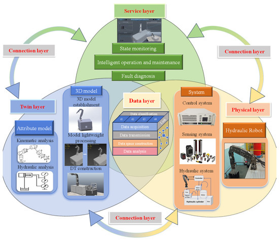
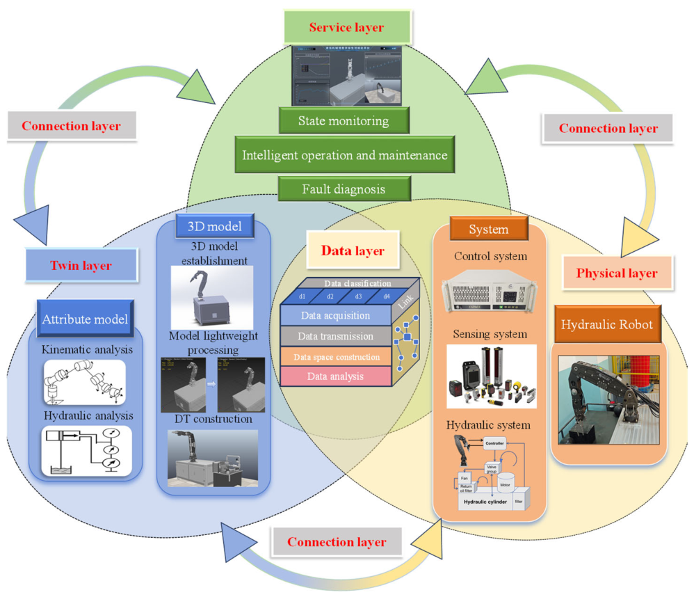
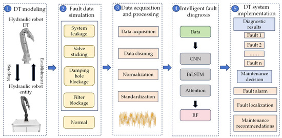
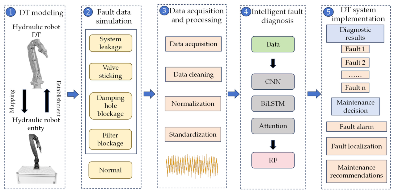
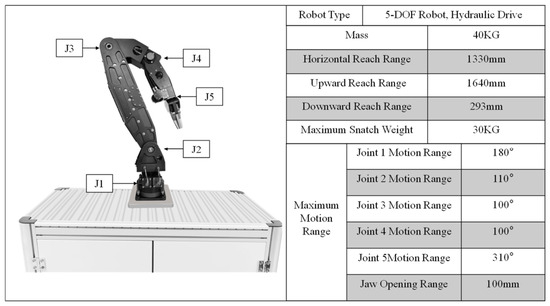
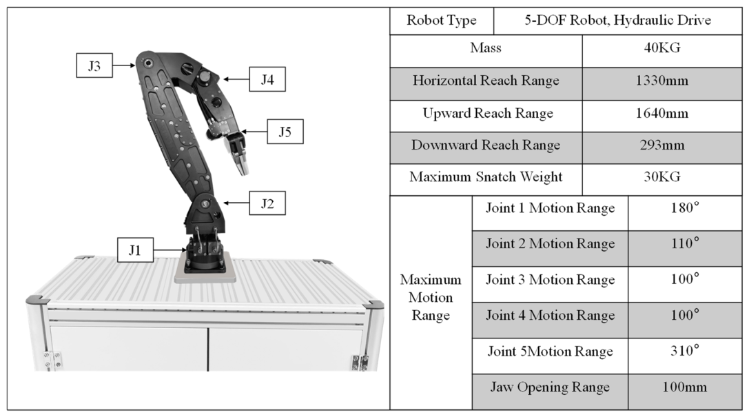
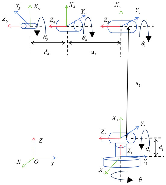
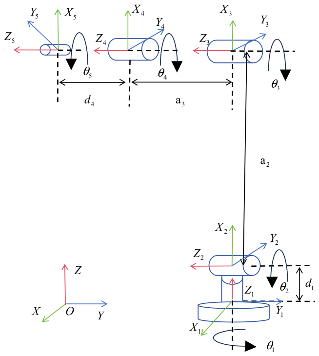
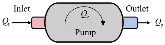
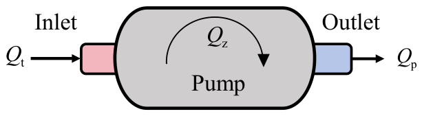
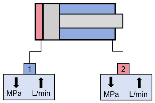
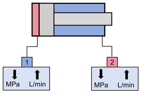
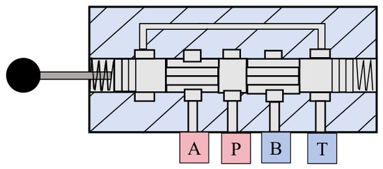
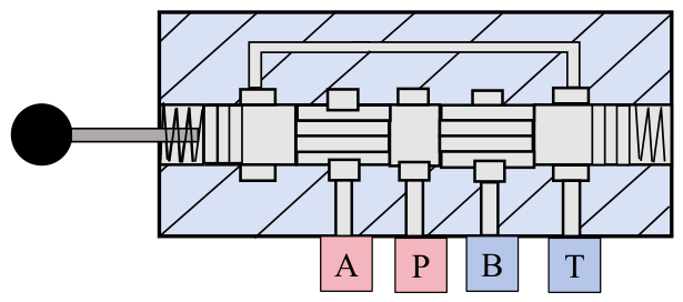
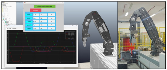
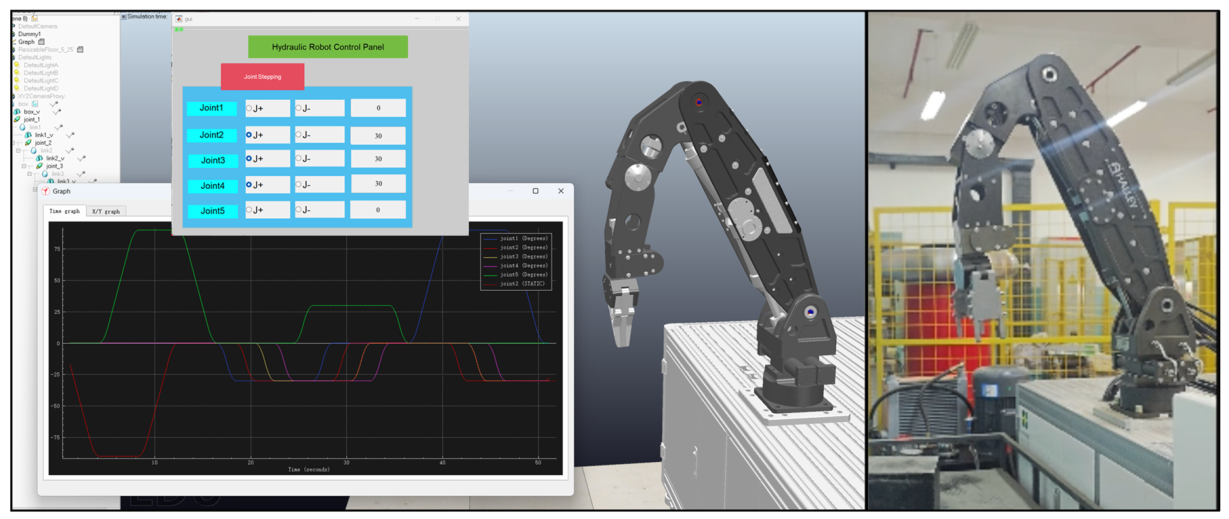
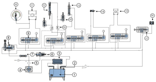
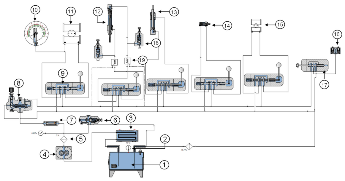
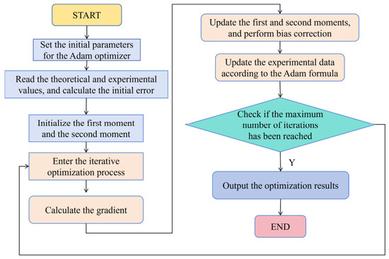
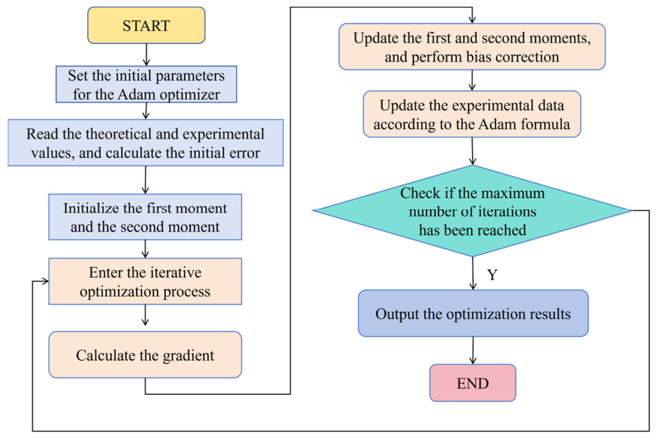
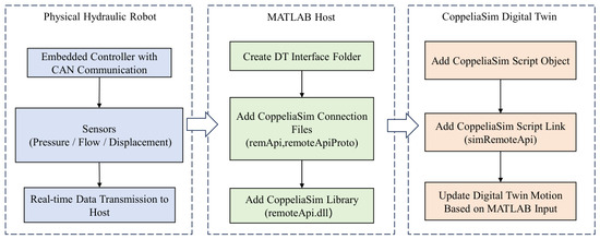
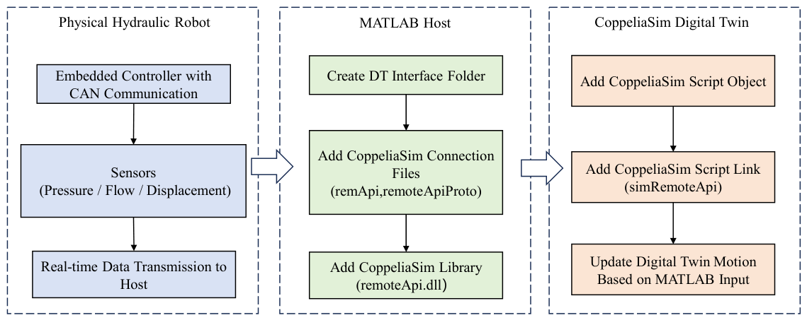
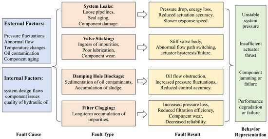
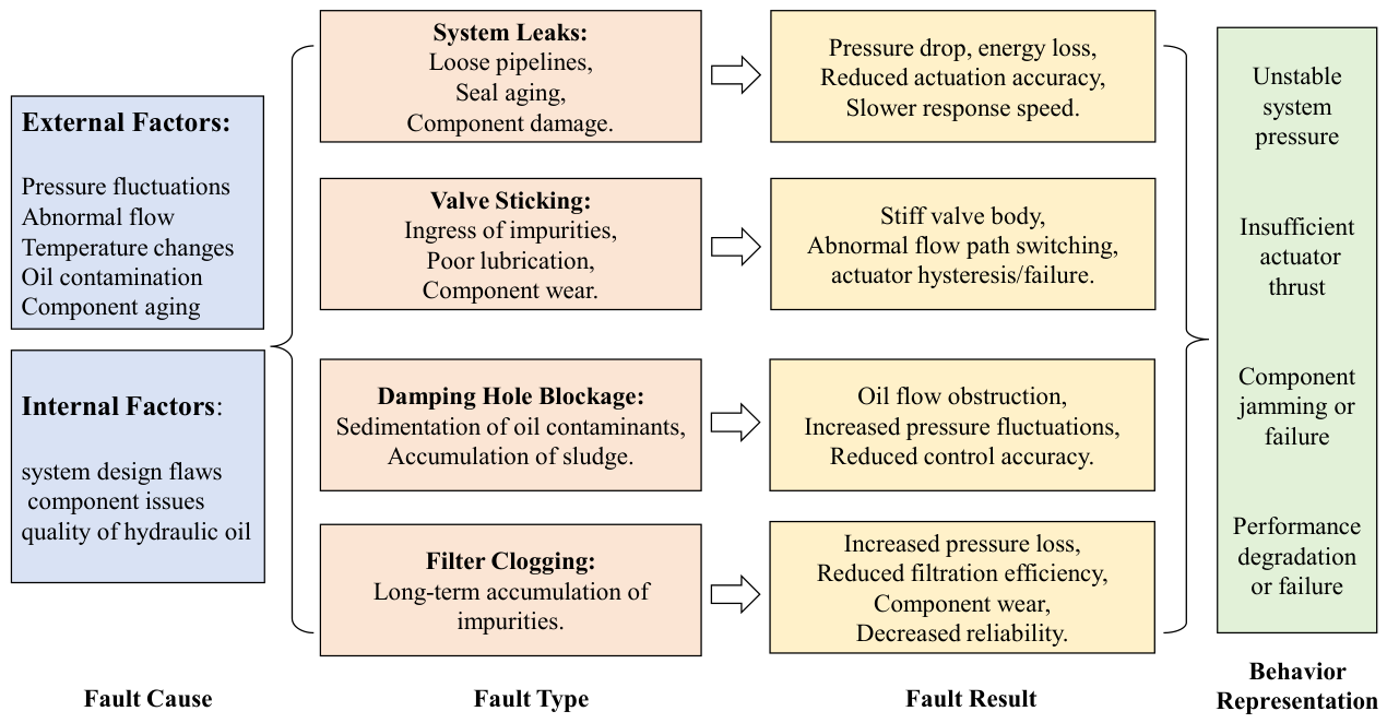
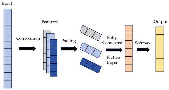
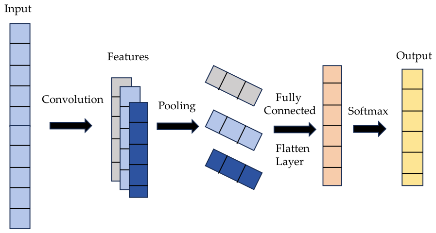
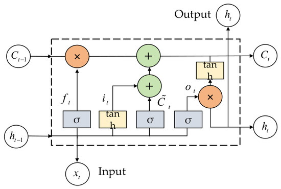
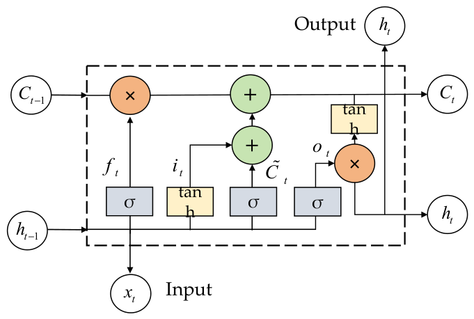
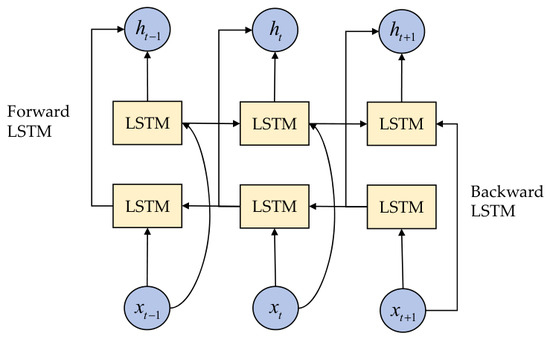
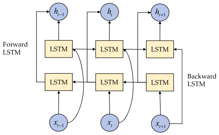
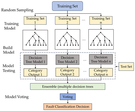
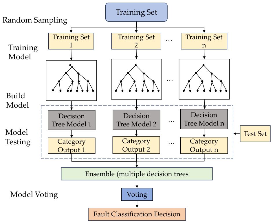
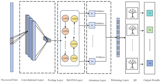
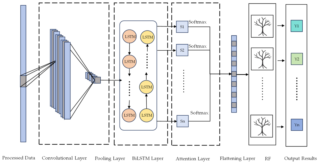
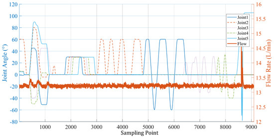
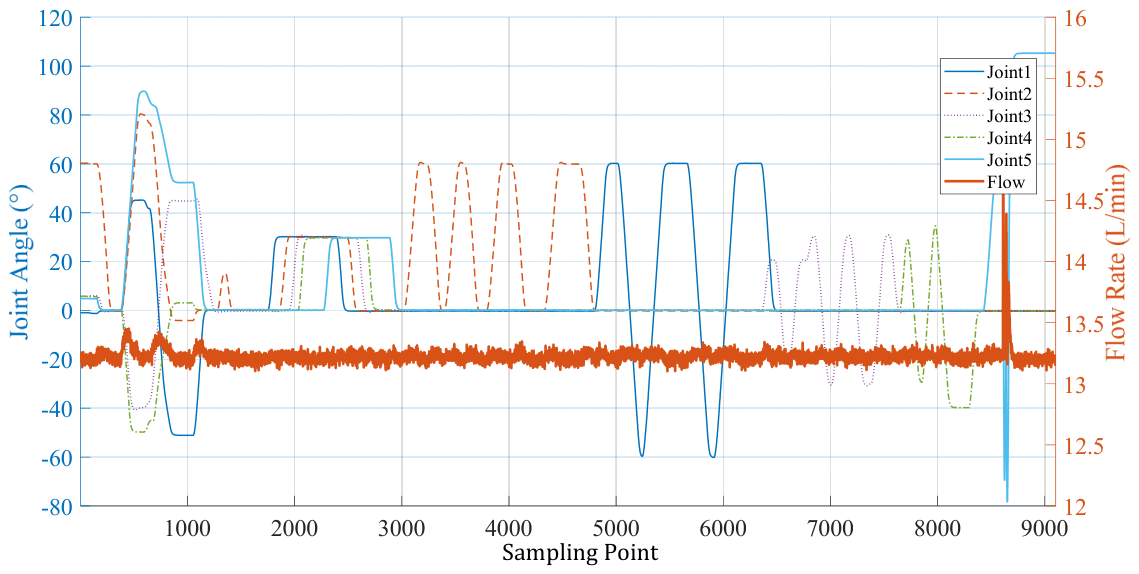
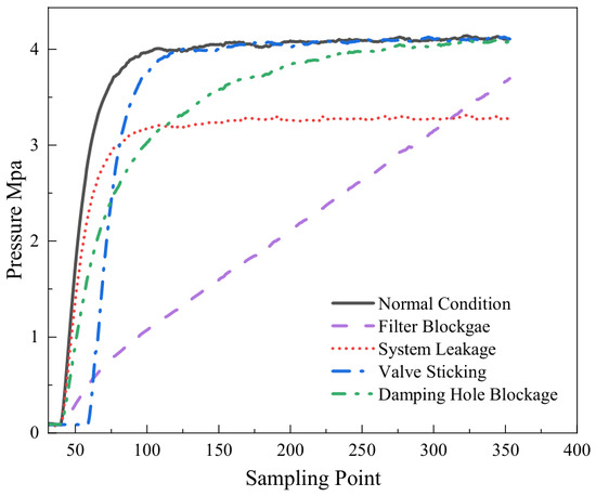
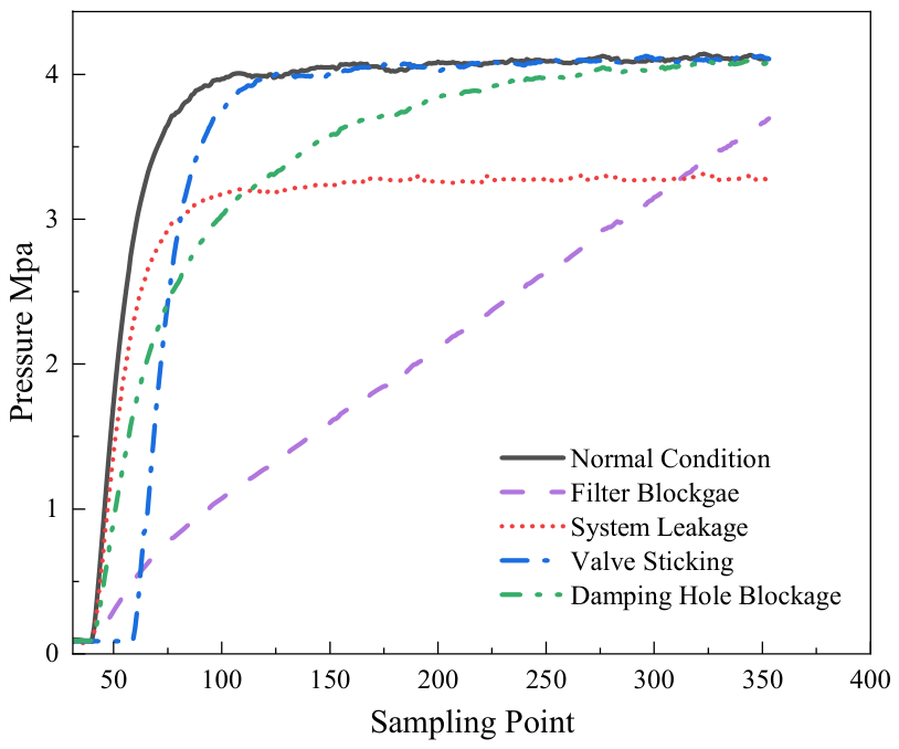
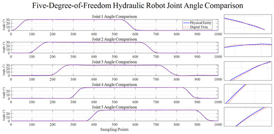
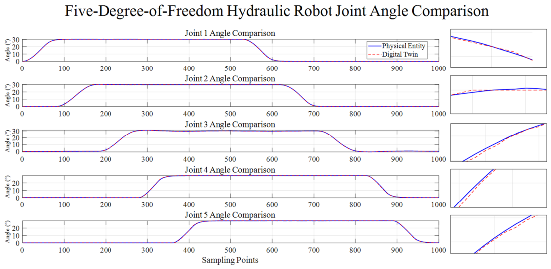
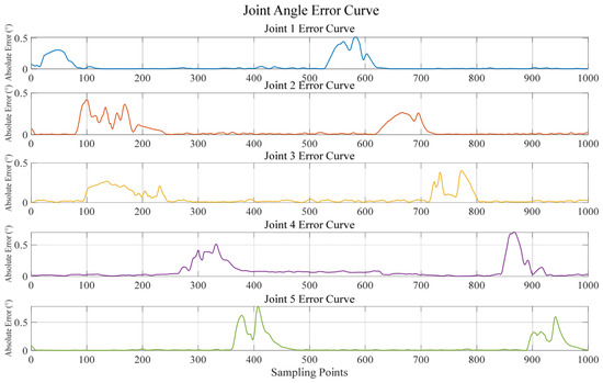
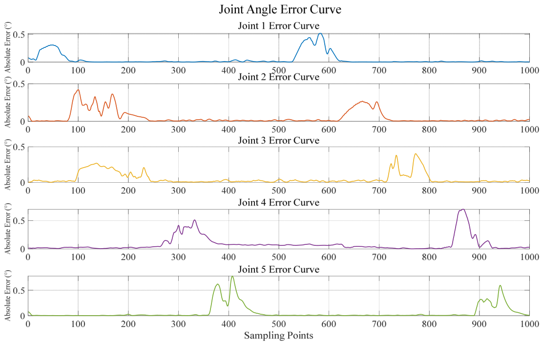
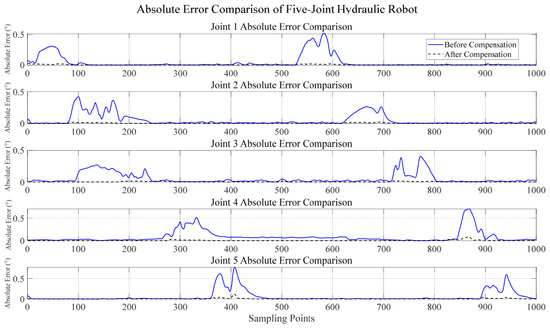
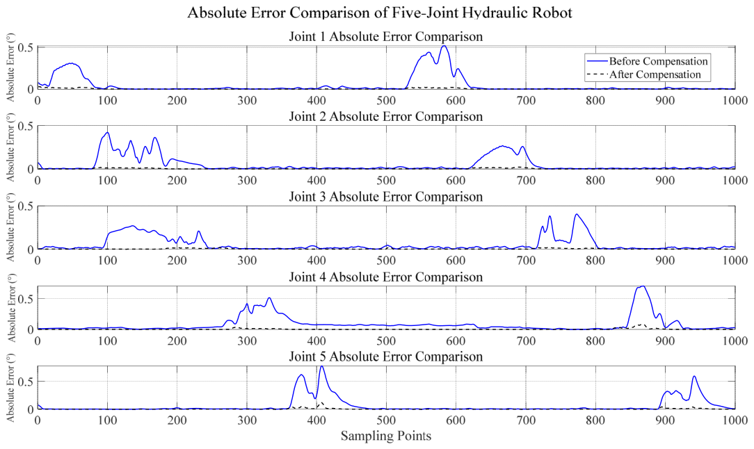
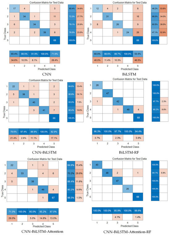
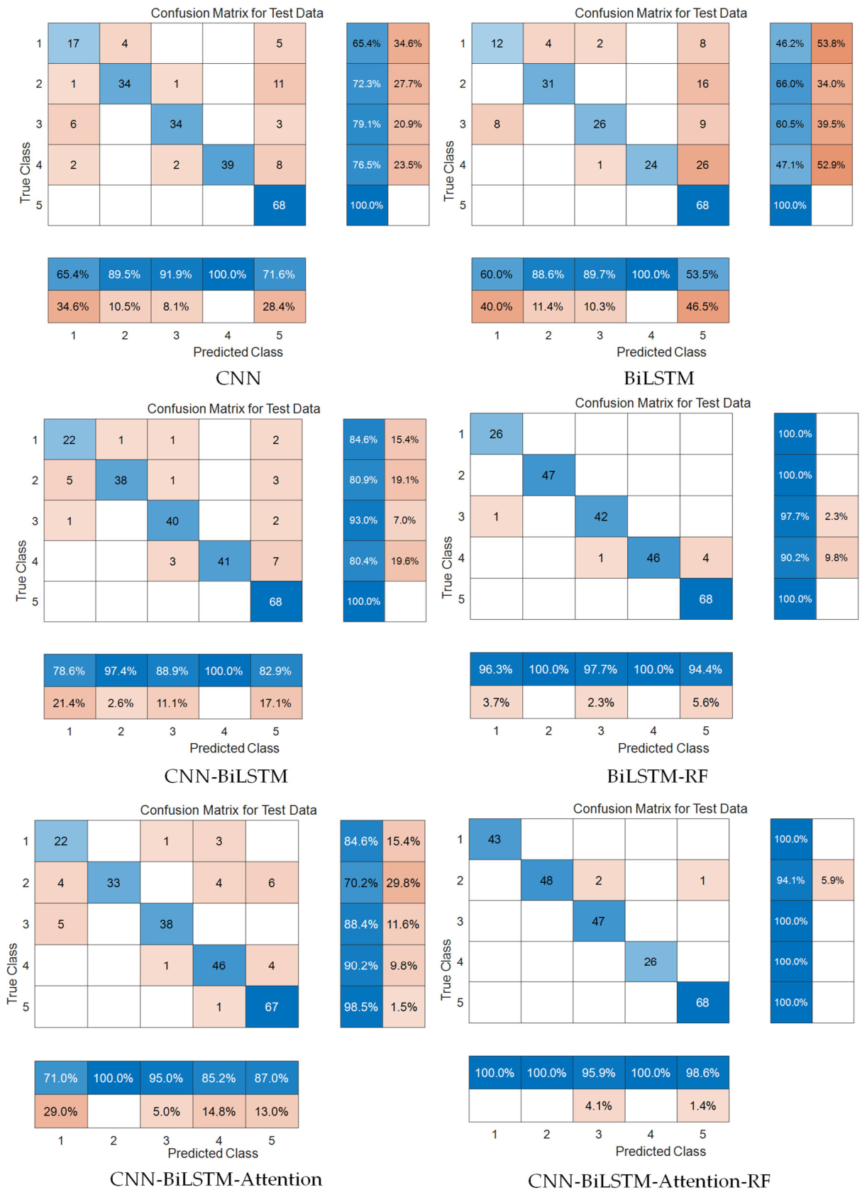
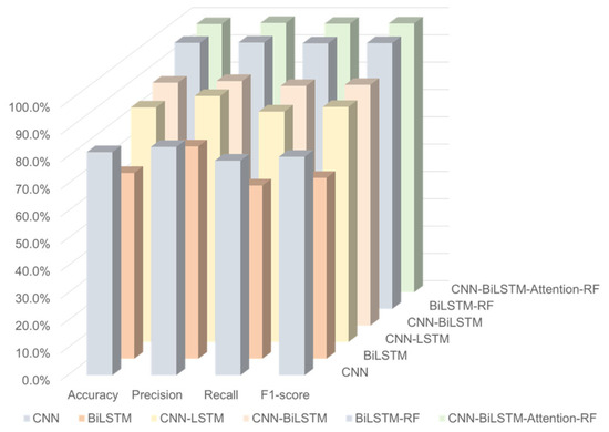
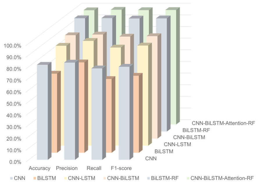

Disclaimer/Publisher’s Note: The statements, opinions and data contained in all publications are solely those of the individual author(s) and contributor(s) and not of MDPI and/or the editor(s). MDPI and/or the editor(s) disclaim responsibility for any injury to people or property resulting from any ideas, methods, instructions or products referred to in the content. |
© 2026 by the authors. Licensee MDPI, Basel, Switzerland. This article is an open access article distributed under the terms and conditions of the Creative Commons Attribution (CC BY) license.