Article

Hierarchical Cooperative Trajectory Planning for Air–Ground Robotic Systems in Communication-Constrained Urban Canyons

1
International School, Beijing University of Posts and Telecommunications, Beijing 100876, China
2
Key Laboratory of Autonomous Transportation Technology for Special Vehicles, Ministry of Industry and Information Technology, School of Transportation Science and Engineering, Beihang University, Beijing 100191, China
3
School of Intelligent Engineering and Automation, Beijing University of Posts and Telecommunications, Beijing 100876, China
4
School of Vehicle and Mobility, Tsinghua University, Beijing 100084, China
*
Author to whom correspondence should be addressed.
Machines 2026, 14(6), 594; https://doi.org/10.3390/machines14060594
Submission received: 18 April 2026 / Revised: 19 May 2026 / Accepted: 20 May 2026 / Published: 26 May 2026
(This article belongs to the Section Robotics, Mechatronics and Intelligent Machines)

Abstract

Heterogeneous airground robotic systems, which integrate unmanned ground vehicles and unmanned aerial vehicles, have shown significant potential in complex autonomous missions. However, when deployed in urban canyons, dense high-rise buildings impose severe communication constraints on ground vehicles, necessitating the introduction of aerial vehicles as relays to maintain reliable connectivity. The resulting cooperative trajectory planning problem is challenging for three reasons. First, the kinematic and communication constraints are tightly coupled. Second, the optimization landscape is highly non-convex and non-differentiable. Third, the planner must balance topological exploration with real-time efficiency. To address these challenges, we propose a hierarchical cooperative trajectory planning framework for an air–ground robotic system. Specifically, in the upper layer, a heuristic-search-guided reinforcement learning mechanism is employed to narrow the search space and circumvent the sparse reward problem, rapidly generating an initial solution. Subsequently, the lower-layer planner utilizes an optimization-based solver, together with a corridor-based constraint formulation method, to refine the initial solution into a kinematically feasible cooperative trajectory. Ultimately, this strategy improves real-time efficiency while improving the quality of feasible cooperative trajectories. Extensive ablation studies and comparative experiments with representative baselines demonstrate that the proposed framework improves collision avoidance, communication reliability, trajectory smoothness, and computational efficiency in the tested urban canyon scenarios.

1. Introduction

Heterogeneous multi-robot collaboration, driven by recent advancements in autonomous robotics, has emerged as a promising paradigm for multi-agent trajectory planning [1]. Among various configurations, the air–ground cooperative system—integrating UAVs and UGVs—has attracted considerable attention due to its complementary mobility and payload capabilities. Accordingly, cooperative trajectory planning for such systems has become a critical research focus, with broad applications in last-mile delivery [2], disaster search and rescue [3], and large-scale environmental monitoring [4].
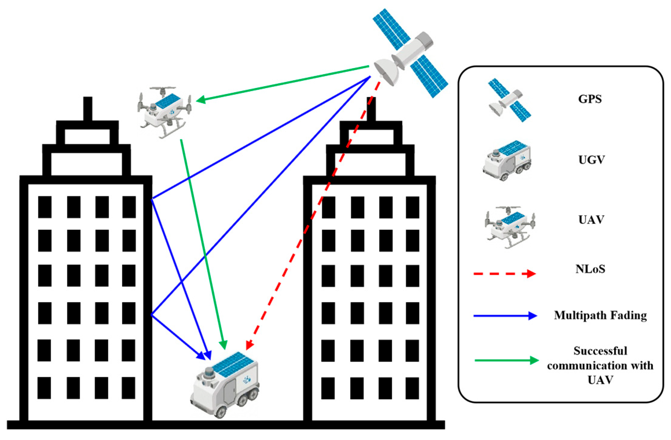
However, deploying UGV-UAV systems in dense urban areas introduces unique spatial challenges, especially in urban canyons. An urban canyon typically refers to a narrow street flanked by continuous high-rise buildings [5]. Such environments can severely degrade UGV communication due to non-line-of-sight (NLoS) propagation [6] and multipath fading [7], which consequently hinder reliable data exchange and real-time localization. To address this issue, a UAV can be deployed as an aerial relay. Benefiting from its high mobility and elevated position, the UAV can help re-establish a stable communication link between the UGV and external infrastructure, as shown in Figure 1. Therefore, a tailored cooperative planning framework is important for supporting both operational safety and planning efficiency in such constrained environments.
In the proposed system, the UAV is assumed to be docked on the UGV and is deployed as an aerial relay only when the UGV encounters a communication failure. Once deployed, the UAV is assumed to maintain connectivity with external infrastructure, thereby providing a reliable communication link for the integrated system. In our study, the LoS/NLoS state is used as a binary geometric connectivity indicator at the trajectory planning level, mainly to capture building-induced blockage between the UGV and UAV. This assumption is suitable when blockage is the dominant factor affecting communication and the relay distance remains within the operational range. However, it may become invalid when distance-dependent path loss, severe multipath fading, strong interference, dynamic blockage, adverse weather, or antenna-related constraints dominate the link quality. In such cases, a more detailed physical-layer channel model should be incorporated for link-quality-aware planning.
Despite the advantages of the UGV-UAV system, cooperative trajectory planning for the UGV-UAV system in an urban canyon still faces the following three core challenges.
First, cooperative trajectory planning for the UGV-UAV under multiple constraints in urban canyons presents significant challenges. In such complex 3D environments, both the UGV and the UAV must avoid obstacles. They also need to satisfy their own kinematic constraints and maintain a stable communication link. Under such multiple constraints, we need to generate a high-quality cooperative trajectory, which remains a challenging task for this research.
Second, the optimization problem formulated from the aforementioned complex scenarios exhibits pronounced non-convexity and non-differentiability. Urban canyons contain complex obstacle topologies. In addition, the UGV and UAV are coupled through kinematic and communication constraints. These factors create many local minima in the high-dimensional search space and make the problem highly non-convex. Furthermore, the inclusion of hard physical limits within the kinematic and communication constraints inevitably introduces non-smooth functions into the optimization framework, leading to a high degree of non-differentiability.
Third, striking a balance between topological exploration and real-time efficiency poses a significant challenge when solving the aforementioned complex optimization problem. To improve topological search capability, the computational complexity of conventional trajectory-searching algorithms increases substantially within the intricate topology of urban canyons, thereby potentially compromising real-time performance. Conversely, traditional optimization-based methods are often used to maintain real-time responsiveness. However, in complex environments, they are prone to local optima. This may degrade the quality and feasibility of the resulting trajectories.
To address the challenges outlined above, we propose a hierarchical framework. In the first stage, a guided RL algorithm is developed to navigate the strong non-convexity and non-differentiability of the optimization problem by leveraging the heuristic nature of the reward function, thereby yielding an initial solution. In the second stage, this solution serves as a warm start for an optimization-based solver, which refines the trajectory for smoothness and obstacle avoidance, enhancing real-time computational efficiency. The main contributions of this paper are summarized in the following three aspects.
  • The UGV-UAV cooperative trajectory planning problem is decoupled into a hierarchical computational framework. A guided RL algorithm first derives a high-quality initial solution that mitigates the adverse effects of non-convexity and non-differentiability. This initial solution then serves as a warm start for an optimization-based solver, thereby enhancing real-time performance while improving the quality of feasible solutions.
  • We introduce a heuristic search algorithm as prior guidance for the RL agent. The heuristic search provides feasible reference paths in complex topological spaces. Based on this guidance, the RL agent explores a reduced search space. This design helps alleviate the sparse-reward problem caused by complex obstacle configurations and improves the efficiency of initial solution generation.
  • To further enhance solver efficiency, a corridor-based constraint formulation method is integrated into the optimization-based solver. This method transforms the original non-convex obstacle avoidance constraints into a set of convex safe corridors, enabling the solver to operate within convex domains and reducing computational overhead for real-time trajectory generation.
The rest of this article is structured as follows. Section 2 reviews the primary research leading up to cooperative trajectory planning of the UGV-UAV system. Section 3 provides the problem statement of our planning task. Section 4 introduces our framework from a macroscopic perspective, while Section 5 elaborates on our framework, including the core motivations and algorithms. Section 6 presents the simulation results and experimental results. Section 7 discusses the necessity of the proposed hierarchical framework through ablation studies and analyzes the limitations of the current work. Finally, Section 8 concludes the paper and outlines future research.

2. Related Research

This Section reviews studies related to cooperative trajectory planning for UGV-UAV systems. We first discuss trajectory planning methods for individual UGVs and UAVs. These methods provide the methodological basis for UGV-UAV cooperative planning. We review the research on cooperative trajectory planning of the UGV-UAV system. Additionally, the primary research within the context of urban canyon environments is introduced.

2.1. Trajectory Planning for UGVs or UAVs

This section primarily categorizes existing research on trajectory planning techniques for UGVs and UAVs into three major paradigms: search-based methods, optimization-based methods, and learning-based methods.
First, search-based methods operate by discretizing the environment into a graph or grid, utilizing graph-search algorithms to systematically find a collision-free geometric path. Specifically, Meng et al. [8] proposed a parameter-optimized Artificial Potential Field A* algorithm for unmanned aerial vehicles in workshop environments, which enhances the standard A* approach by integrating a variable step-size strategy and potential field values into the cost function to dynamically improve planning accuracy and flight stability.
Second, optimization-based methods formulate trajectory generation as a mathematical programming problem, optimizing objectives such as smoothness while strictly satisfying the vehicle’s kinematic constraints. Specifically, for UGVs, Qiao et al. [9] and Bao et al. [10] utilized mathematical programming to generate smooth, kinematically feasible trajectories by balancing energy efficiency and integrating landmark-based localization, respectively. Extending these principles to network scale, Chen et al. [11] formulated a coordinated routing policy for connected vehicles to optimize system-wide travel efficiency alongside individual trajectory smoothness. Furthermore, for UAVs, Wu et al. [12] developed a trajectory-based flight scheduling framework for UAVs in AirMetro systems, mathematically guaranteeing collision-free and efficient urban airspace operations.
Third, learning-based methods leverage data-driven models to map environmental observations directly to planning decisions, enabling highly adaptive and real-time responses in complex scenarios. Specifically, in the context of UGVs, Ayalew et al. [13] applied deep RL techniques to mobile robots, demonstrating how data-driven policies can dynamically adjust paths to handle environmental uncertainties and dynamic obstacles. Pushing the boundaries of these learning models to UAVs, Du et al. [14] proposed a cooperative pursuit framework for intercepting unauthorized UAVs in urban airspace, showcasing the real-time decision-making and adaptive capabilities of learning algorithms in highly dynamic, multi-agent adversarial environments.

2.2. Cooperative Trajectory Planning of UGV-UAV System

This section primarily categorizes existing research on cooperative trajectory planning of UGV-UAV systems into three major scenarios: UGV-aided UAV trajectory planning, UAV-aided UGV trajectory planning, and reciprocal UGV-UAV cooperative trajectory planning.
First, in UGV-aided UAV scenarios, ground vehicles typically act as mobile depots or edge servers to compensate for the limited battery capacity and computational payload of UAVs. Specifically, UGVs are utilized as mobile docking stations or nested depots to optimize vehicle routing, facilitate autonomous landing, and coordinate large-scale exploration [15,16,17]. Furthermore, UGVs are increasingly deployed as mobile edge computing nodes to provide computational support, providing various frameworks for efficient and secure task offloading in urban surveillance and disaster response missions [18,19].
Second, as for studies of UAV-aided UGV scenarios, aerial platforms serve as overhead scouts or communication relays to assist ground vehicles in obstacle avoidance and pathfinding in GPS-denied or occluded environments. Particularly in the context of overhead scouting, Xie et al. [20] designed collaborative path-planning frameworks where UAVs provide extended environmental visibility to optimize UGV trajectories and hybrid navigation strategies. Expanding beyond physical navigation to communication and operational coordination, Oubbati et al. [21] and Sun et al. [22] utilized aerial platforms to facilitate energy-efficient urban patrolling and joint resource scheduling for mobile edge computing within vehicular networks.
Third, UGV-UAV cooperative planning focuses on joint spatiotemporal optimization. It has been widely applied to last-mile delivery and heterogeneous formation control. In these tasks, the UGV and UAV operate simultaneously to improve task-level performance. In the domain of cooperative logistics and last-mile delivery, Jang et al. [23] and Li et al. [24] proposed dynamic truck-drone routing frameworks that jointly optimize path planning and vehicle scheduling to minimize overall travel costs. Expanding upon this routing paradigm, Yoon et al. [25] introduced an optimal load-balancing strategy for collaborative parcel pickup, while Li et al. [26] extended these joint routing principles to maritime environments through vessel–UAV collaboration. To handle the high-dimensional complexity of such joint missions, Ma et al. [27] applied adaptive graph neural networks for dynamic task allocation, and Zhu et al. [28] developed deep learning-enhanced trajectory predictors for cross-domain vehicle interactions. Conversely, addressing the strict kinematic and stability requirements of heterogeneous formation control, Tian et al. [29], Yan et al. [30], and Liang et al. [31] designed distributed adaptive control methods to ensure robust formation tracking, accommodate asymmetric physical constraints, and maintain prescribed performance even with human-in-the-loop participation.
Recent studies have also emphasized the importance of reliable state estimation and hierarchical planning in robotic systems. For example, Cosenza et al. [32] developed a virtual-sensor-based wheel angular-speed estimation method for differential-drive robots, showing that accurate motion-state estimation is important for reliable control and trajectory tracking. However, these studies mainly focus on single-robot planning, autonomous driving, or general hierarchical decision-motion coupling, and rarely consider UGV-UAV cooperative trajectory planning under simultaneous communication, obstacle avoidance, and heterogeneous kinematic constraints in urban canyon environments. Therefore, a dedicated hierarchical framework is still needed for communication-constrained air–ground cooperative planning.

2.3. Research on Urban Canyons

Research on urban canyon environments includes methods to improve GNSS positioning accuracy [33], techniques for signal correction [34] and optimization of planned trajectories [35]. In contrast, this paper primarily focuses on trajectory planning research under communication-constrained conditions within urban canyons.

3. Problem Statement

Essentially, our cooperative planning task can be formulated as an OCP subject to multiple constraints. Its core objective is to determine an optimal state sequence X * = x g , x a and a corresponding optimal control sequence U * = u g , u a to minimize the cost function, while satisfying the requirements of system kinematics, communication quality, and collision avoidance. The state sequence is defined as X = x g , x a , where the UGV state vector is x g = [ p g x , p g y , ψ g , v g ] T and the UAV state vector is defined as x a = [ p a x , p a y , p a z , ϕ a , θ a , ψ a ] T . The control sequence is defined as U = u g , u a , consisting of the UGV control vector u g = [ a g , δ g ] T and the UAV control vector u a = [ v a x , v a y , v a z , ω a x , ω a y , ω a z ] T . In the following sections, the formulation of this OCP will be elaborated. For clarity and consistency, we provide a notation table for all state and control variables, as shown in Table 1.

3.1. Cost Function

To ensure rapid planning task completion, guarantee communication quality in urban canyons and enhance the smoothness of the trajectory, the cost function J is formulated as follows:
J = w t ( k N k 0 ) Δ t + k = 0 N 1 ( w c J c o m m k + w s J s m o o t h k )
Specifically, the planning task time cost is denoted by ( k N k 0 ) Δ t , where k 0 and k N represent the initial and terminal step index, respectively; Δ t represents the time interval of each step; by tuning the weight coefficients w t , w c and w s , the cost function can be adapted to accommodate different planning task priorities; the communication quality cost J c o m m k is defined as
J c o m m k = γ , if   Line ( p g k , p a k ) O 0 , otherwise
where p g k and p a k denote the positions of the UGV and UAV at step k , respectively; Line ( ) O indicates whether the line segment between the UGV and UAV intersects the set of building obstacles O ; and γ represents the penalty constant associated with communication occlusion. The trajectory smoothness cost, J s m o o t h k , is defined as
J s m o o t h k = u g k 2 + u a k 2
where u g k and u a k denote the control vectors of the UGV and the UAV at step k , respectively.

3.2. Constraints

To guarantee the physical feasibility of the cooperative trajectories and ensure operational safety within complex urban environments, the formulated OCP must satisfy the following five constraints.

3.2.1. Two-Point Boundary Value Constraints

The two-point boundary value constraints are defined as
p g 0 = p s t a r t , v g 0 = 0 ;   p a 0 = p s t a r t , v a 0 = 0
p g N p g o a l ε , v g N = 0 ;   v a N = 0
where p g 0 and p a 0 denote the starting points of the cooperative trajectories for the UGV and UAV, respectively; p s t a r t represents the starting coordinates in the map; v g 0 and v a 0 represent the initial velocities of the UGV and UAV; p g N and p a N denote the terminal points of the cooperative trajectories; v g N and v a N represent the terminal velocities of the UGV and UAV; and ε denotes the terminal tolerance.

3.2.2. Kinematic Constraints

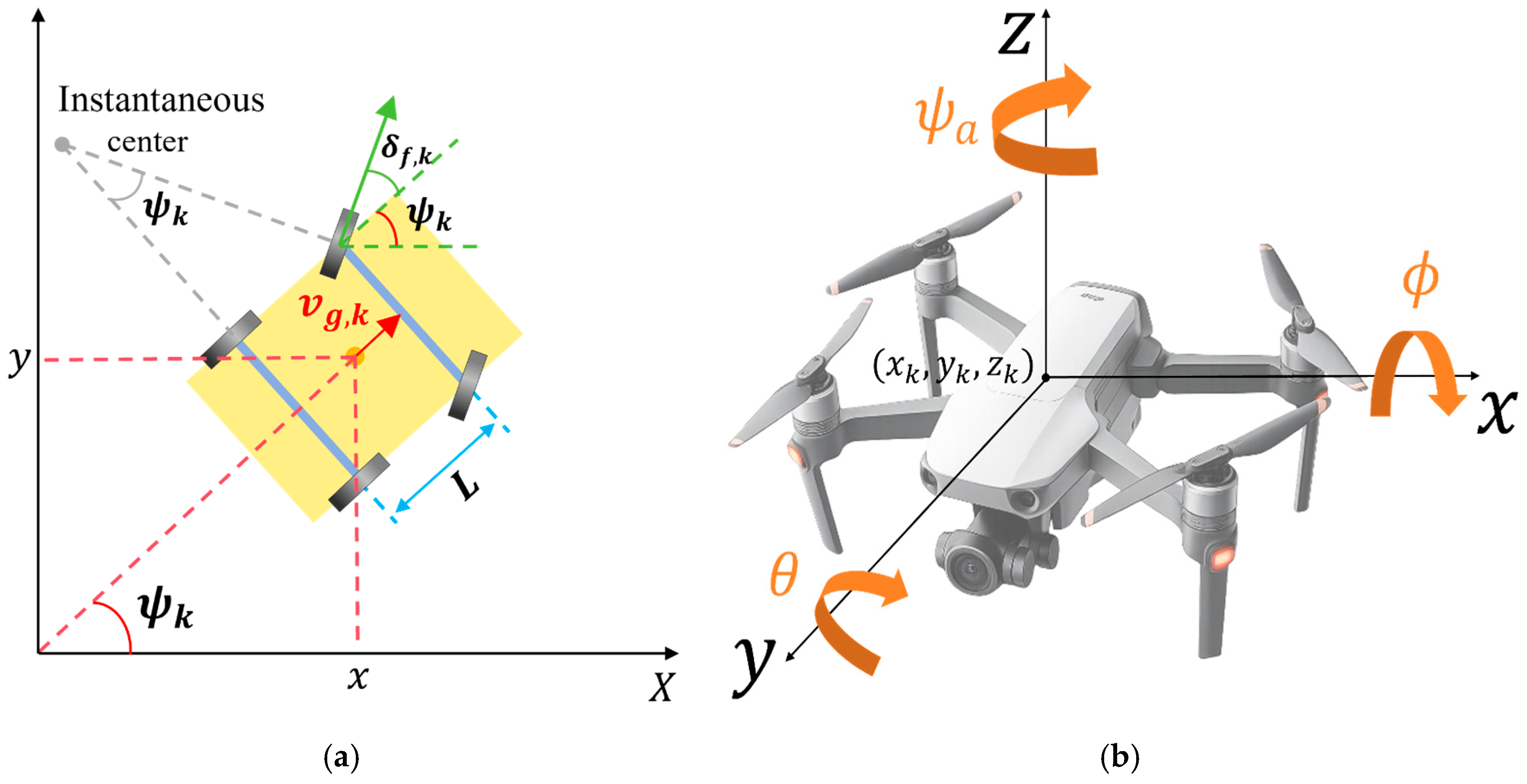
The state transitions of both the UGV and UAV at each time step must be governed by the discrete-time kinematic equations x g , a k + 1 = f ( x g , a k , u g , a k ) . For the UGV, the kinematic bicycle model is employed as presented in Figure 2a, and the specific equations are formulated as follows:
x g k + 1 = x g k + v g k cos ( ψ g k ) Δ t y g k + 1 = y g k + v g k sin ( ψ g k ) Δ t ψ g k + 1 = ψ g k + v g k L tan ( δ k ) Δ t v g k + 1 = v g k + a g k Δ t
where ψ g k and δ k denote the heading angle and the front wheel steering angle of the UGV at the k -th step, respectively; a g k represents the acceleration of the UGV at the k -th step; L is the wheelbase of the UGV; and Δ t denotes the time interval between discrete steps.
For the UAV, the quadrotor model is adopted as presented in Figure 2b, and the specific equations are formulated as follows:
p a k + 1 = p a k + v a k Δ t χ a k + 1 = χ a k + T a k ω a k Δ t
where p a k = [ p a x k , p a y k , p a z k ] T denotes the position vector of the UAV; χ a k = [ ϕ a k , θ a k , ψ a k ] T represents the attitude vector, where ϕ a k , θ a k , and ψ a k correspond to the roll (around the x -axis), pitch (around the y -axis), and yaw (around the z -axis) angles, respectively; v a k represents the linear velocity vector of the UAV, and ω a k denotes the angular velocity vector in the body-fixed frame; Δ k is the discretized time step; the transformation matrix T a k from the body-frame angular velocities to the Euler angle rates is defined as
T a k = 1 tan θ k sin ϕ a k tan θ k cos ϕ a k 0 cos ϕ a k sin ϕ a k 0 sin ϕ a k / cos θ a k cos ϕ a k / cos θ a k
To prevent the cooperative trajectories from violating physical laws of motion, the velocities and control vectors of both the UGV and UAV must satisfy the following physical constraints
v g v min , v max ,   a g a min , a max ,   δ g δ g , max
v a , x y v x y , m a x ,   | v a , z | v z , m a x ,   ω a ω a , m a x
where ω a = [ ω a x , ω a y , ω a z ] T denotes that the magnitude of the angular velocity vector of the UAV is bounded by its maximum allowable value ω m a x to ensure flight stability and satisfy actuator limits.

3.2.3. Collision Avoidance Constraints

The collision avoidance constraint is defined below
p g k C g k ,   p a k C a k
where C g k , C a k represents the UGV/UAV safety corridor generated by the algorithm at the k -th step, the specific procedure of which will be elaborated in detail in Section 5.

3.2.4. Communication Range Constraints

The communication range constraint is defined below
p a k p g k D max
where D m a x represents the maximum allowable communication distance between the UGV and the UAV.

3.3. Remarks

Integrating the above-mentioned components, the cooperative trajectory planning problem in this paper can be summarized in the following form:
min x ( t ) , u ( t ) , T   ( 1 ) , s . t .   Kinematic   constraints   ( 6 ) ( 10 ) ;               Boundary   constraints   ( 4 )   and   ( 5 ) ;               Collision avoidance   constraints   ( 11 )   and   ( 12 ) .
Directly solving the UGV and UAV trajectories independently using traditional path planning algorithms and corridor constraints [36] may not be suitable for the formulated problem. First, the communication constraint depends on the relative positions of the UGV and UAV and, therefore, introduces a nonlinear coupling between their trajectories. Second, the UGV and UAV follow different kinematic models, so independent planning cannot easily guarantee joint feasibility of the complete state-control sequence. Third, in a non-convex environment, a heuristic initial solution may constrain the optimizer to a limited feasible region, which can reduce the quality of the final cooperative trajectory.

4. Overall Framework

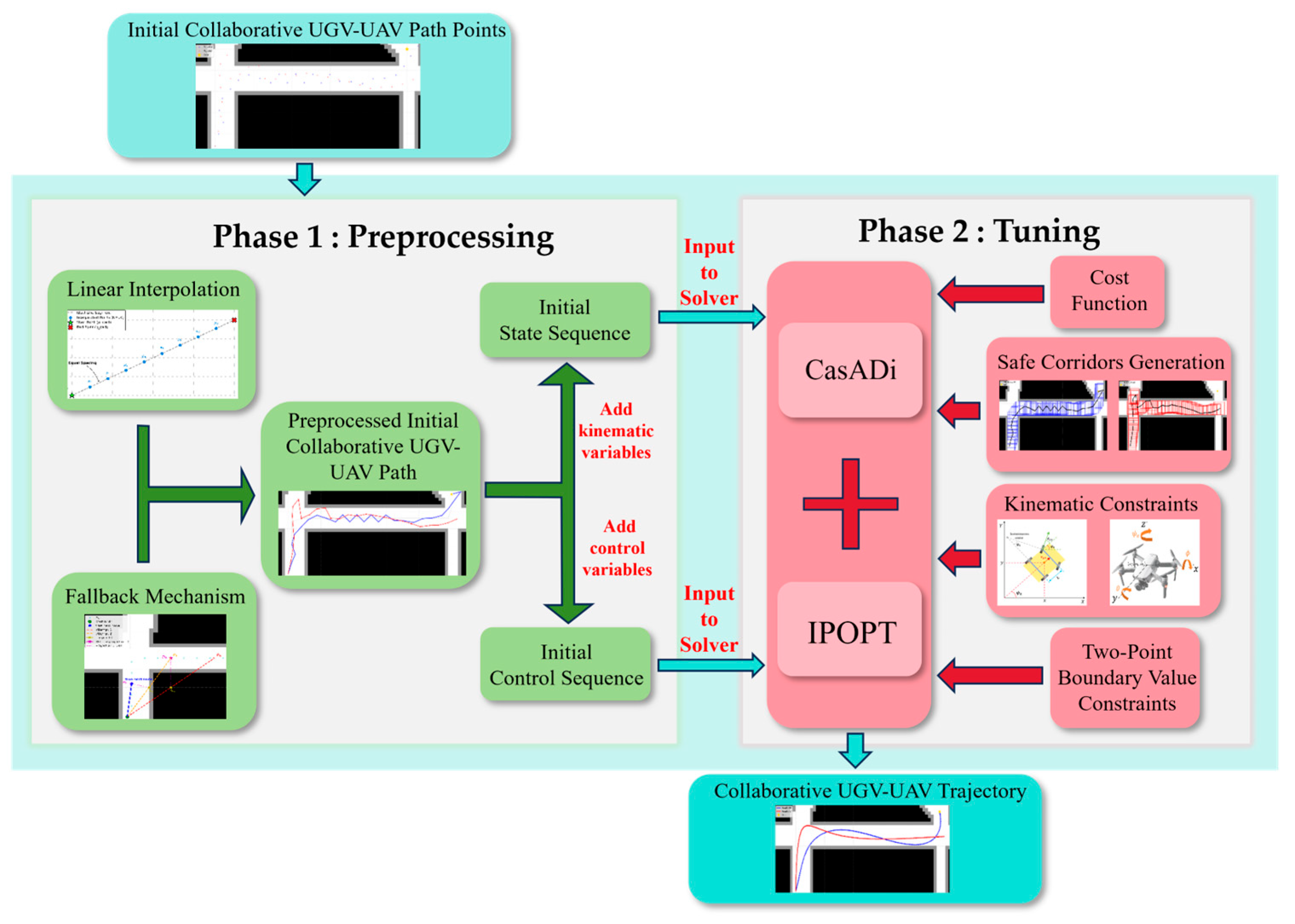
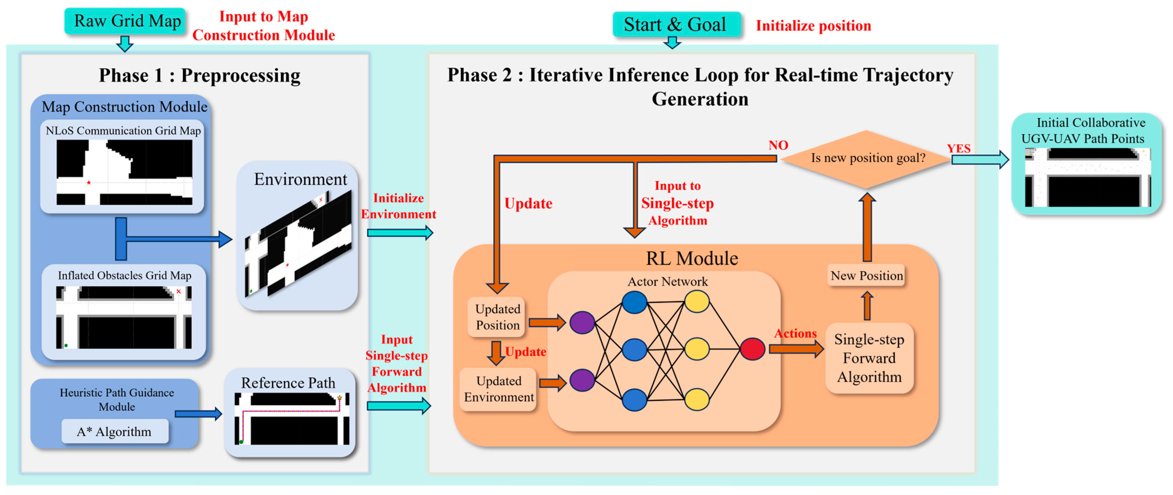
This Section presents the design motivation and detailed architecture of the proposed two-layered planning framework, as presented in Figure 3. Furthermore, it elaborates on how this framework is applied to solve the aforementioned UGV-UAV cooperative trajectory optimization problem in urban canyon environments.

4.1. Motivation

Inspired by the closed-loop mechanism of forward decision-making guidance and backward motion planning [37], a hierarchical cooperative planning framework is proposed to address the optimization problem formulated in Section 3.
In the upper layer, the strong non-convexity and non-differentiability of the problem render conventional optimization-based solvers highly susceptible to local optima. RL is therefore adopted, as it circumvents direct mathematical resolution through trial-and-error interactions with the environment. However, pure RL in complex urban canyon scenarios suffers from the sparse reward dilemma. Drawing on the from-coarse-to-fine paradigm [38], the A* algorithm is introduced to pre-generate a reference path as prior guidance, narrowing the search space and contributing to more stable RL training.
In the lower layer, since the upper-layer output typically violates certain complex constraints and lacks spatial smoothness, an optimization-based solver is employed for trajectory refinement. A safe corridor generation algorithm is further incorporated to transform non-convex obstacle-avoidance constraints into convex formulations, supporting collision-free guarantees while optimizing kinematic smoothness.

4.2. Two-Layered Planner

This study proposes a two-layered trajectory planning framework, which decouples the UGV-UAV cooperative trajectory planning problem into a discrete spatial exploration phase and a continuous numerical optimization phase. This approach enables the system to efficiently narrow down the search space prior to control execution, thereby achieving a balance between search efficiency and trajectory quality.
In the upper-layer framework, this study designs an initial trajectory generation strategy based on RL guided by heuristic search. The input to this layer consists of the environmental grid map, the encoded communication-connectivity map, and the start and goal configurations of the UGV. The corresponding output is a sequence of discrete waypoints for both the UGV and UAV that preliminarily satisfy the cooperative constraints.
In the lower-layer framework, this study formulates a trajectory optimizer based on nonlinear programming (NLP). The input to this layer consists of the initial cooperative waypoint sequence from the upper layer, along with the OCP cost function and constraints. The corresponding output is the refined feasible UGV-UAV cooperative trajectory.
The upper and lower layers achieve cooperative trajectory planning through the coordination of topological guidance and a warm-start mechanism. In highly non-convex environments, the traversable space is fragmented into multiple homotopy classes. While lower-layer NLP solvers excel at local refinement, they are not designed to perform topological transitions across obstacles. However, by directly utilizing the upper layer’s topologically informative initial trajectory as a warm-start input, the lower-layer solver reduces reliance on unguided local search. Since this initial solution is expected to lie closer to the optimum, the NLP solver only needs to handle the complex kinematic constraints of the UGV and UAV within the established safe corridor. This enables the algorithm to generate an optimal cooperative trajectory within minimal iterations.

5. Methodology

This Section elaborates on the specific architecture, operational logic, and algorithmic principles of the key modules within the proposed two-layer planner.

5.1. Upper-Layer Planner

The upper-layer planner consists of four modules designed to generate initial waypoint sequences P i n i t = { ( p g , i n i t k , p a , i n i t k ) } k = 0 N with topological guidance in urban canyon environments. In the following sections, we will sequentially introduce the constituent components of the upper-layer planner, its operational pipeline, the key RL algorithm employed, and the associated training network architecture.

5.1.1. Components and Operational Pipeline

The upper-layer planner is designed to generate an initial cooperative waypoint sequence with topological guidance in urban canyon environments, as shown in Figure 4. It consists of four tightly coupled modules: map construction, heuristic path guidance, reinforcement learning, and the DRL network.
First, the map construction module establishes a two-layered environmental representation. The first layer is an inflated 3D grid map M o b s H × W × L constructed from a manually curated polygonal dataset based on Google Earth real-world imagery, where grid values of 1 and 0 represent obstacles and free space, respectively. The second layer is an NLoS communication grid map M n l o s H × W × L . Unlike M o b s , which is assumed to be a given urban canyon scenario, M n l o s is dynamically updated during RL inference according to the current UGV position. Specifically, the LoS status between the UGV and UAV is evaluated based on M o b s , where 0 indicates visible and 1 indicates occluded. Therefore, M n l o s is updated as the UGV moves.
Second, the heuristic path guidance module employs the A* algorithm to generate a 2D reference path P r e f , g = { p g , t arg e t 0 , p g , t arg e t 1 p g , t arg e t N 1 } for the UGV and a 3D reference path P r e f , a = { p a , t arg e t 0 , p a , t arg e t 1 p a , t arg e t N 1 } for the UAV according to the start and goal positions. To prevent colliding with obstacles, a distance transform field is incorporated into the 3D grid map M o b s used by A*.
Third, the RL module treats the UGV and UAV as two cooperative agents in the RL environment S = { S i m g , p g k , p a k } . The image-based state S i m g is constructed by concatenating M o b s and M n l o s . The action space A 5 consists of displacement vectors for the UGV in the XY plane and for the UAV in the XYZ space. The reward function R is mapped from the objective function and constraints of the OCP, which will be elaborated in Section 5.1.2.
Finally, the DRL network adopts an Actor-Critic architecture. The CNN branch extracts features from the S i m g and maps them into a 256-dimensional feature vector, while the MLP branch maps the UGV-UAV position vector into a 64-dimensional representation. These two feature vectors are concatenated into a 320-dimensional mixed feature vector and further transformed into a 128-dimensional latent representation. Based on this representation, the Actor network outputs the UGV and UAV displacement actions, while the Critic network estimates the expected cumulative return to guide policy optimization during training.
During execution, the map construction and heuristic path guidance modules first perform preprocessing for the given scenario. M o b s and M n l o s are generated, and A* is used to obtain P r e f , g and P r e f , a . The planner then enters the iterative RL inference loop. At each discrete time step, the updated S i m g and position vectors are fed into the pre-trained Actor-Critic network. The Actor outputs the cooperative displacement actions, after which the upper-layer planner performs a single-step forward operation in the urban canyon environment and updates the UGV-UAV positions. This process is repeated until the UGV reach the goal. The coordinates recorded at all discrete time steps form P i n i t , which is then passed to the lower-layer planner as the warm-start initial guess.

5.1.2. Forward Planning in RL

Forward planning in RL consists of a sequence of identical computational steps, with the detailed algorithmic logic for each step presented in Algorithm 1, which is described as follows:
At the onset of each discrete time step k , it dynamically retrieves the reference paths P r e f , g and P r e f , a pre-planned by the A* algorithm based on the current spatial coordinates of the UGV and UAV. From these paths, the local target guidance points p g , t a r g e t and p a , t a r g e t for the subsequent stage are extracted. These are completed by function ExtractReferenceTarget ( ) . Subsequently, the spatial positions of the UGV and UAV are updated according to the displacement vectors received from the Actor network, subject to a hard truncation function ClipToMapBoundary ( ) . Finally, a reward value based on the reward function is fed back based on the agent’s updated spatial configurations. The details of the reward function are illustrated as follows:
The objective functions and constraints of the OCP defined in Section 3 are mapped into the RL reward function R t o t a l , as follows:
R t o t a l = R p r o g r e s s + R s a f e t y + R c o m m + R c o n s
Specifically, the first term R p r o g r e s s evaluates navigation efficiency by measuring the reduction in the Euclidean distance between each agent and its corresponding A*-guided target point
R p r o g r e s s = w p , g ( d g k d g k + 1 ) + w p , a ( d a k d a k + 1 )
where d g and d a denote the distances from the UGV and UAV to their corresponding A* reference points, respectively, and w p , g and w p , a are the progress reward weights. R s a f e t y corresponds to the collision constraints prior to corridor generation (which will be illustrated in Section 5.2.3)
R s a f e t y = w c o l l i s i o n , if   p g , a k + 1 O 0 , otherwise
where w c o l l i s i o n represents the collision penalty coefficient, O represents obstacles. R c o m m corresponds to the communication quality cost J c o m m k defined in Section 3. The system queries M n l o s in real time, and a fixed penalty is triggered once the NLoS state appears
R c o m m = w c o m m , if   Line ( p g , p a ) O 0 , otherwise
where w c o m m represents the communication penalty coefficient. R c o n s corresponds to the maximum communication distance constraint defined in Section 3
R c o n s = 0.1 w c o m m p a k p g k D m a x , if   p a k p g k > D m a x 0 , otherwise
Upon computing the reward function, the environment immediately invokes the collision detection procedure. If the trajectory of either the UGV or the UAV is detected by function CheckCollision ( ) for intruding into the obstacle regions within M o b s , the system triggers a ‘soft reset’ strategy. Unlike conventional logic, where collisions lead to immediate episode termination, we forcibly roll back the agents’ coordinates to their nearest A* reference waypoints, which is completed by function RollbackToNearestAStarPoint ( ) . This rollback mechanism effectively concludes the single-step update of the RL process.
Algorithm 1. RL Single-Step Execution Logic
Input: Current coordinates p g k , p a k , reference paths P ref , g , P ref , a , action vectors
Output: Updated coordinates p g k + 1 , p a k + 1 , step total reward R total
1: p g , t arg e t k , p a , t arg e t k ExtractReferenceTarget ( p g k , p a k , P ref , g , P ref , a )
2: // Update positions with boundary truncation
3: p g k + 1 ClipToMapBoundary ( p g k + p g Δ t )
4: p a k + 1 ClipToMapBoundary ( p a k + p a Δ t )
5: // Calculate reward components
6: R progress 0 , R s a f e t y 0 , R comm 0 , R cons 0
7: R progress w p , g ( d g k + 1 d g k ) + w p , a ( d a k + 1 d a k )
8: if  p g k + 1 O  or  p a k + 1 O  then
9:    R safety w collision
10: end if
11: if  Line ( p g k + 1 , p a k + 1 ) O based on M nlos  then
12:    R comm w comm
13: end if
14: if  p a k + 1 p g k + 1 > D max  then
15:    R cons 0.1 w comm ( p a k + 1 p g k + 1 D max )
16: end if
17: R total R progress + R safety + R comm + R cons
18: // ‘Soft reset’ strategy for collision avoidance
19: if  CheckCollision ( p g k + 1 , p a k + 1 , M obs )  then
20:    p g k + 1 RollbackToNearestAStarPoint ( p g k + 1 , P ref , g )
21:    p a k + 1 RollbackToNearestAStarPoint ( p a k + 1 , P ref , a )
22: end if
return  p g k + 1 , p a k + 1 , R total

5.1.3. DRL Training Network

In the upper-layer cooperative planning framework, we train the Actor-Critic network using the Proximal Policy Optimization (PPO) algorithm. At each discrete time step k , the agent acquires the environmental state S k . Based on this state, the old policy network π θ o l d outputs the distribution parameters μ k and σ k to construct a multivariate normal distribution N ( μ k , σ k 2 ) , from which the joint action vector a k for the UGV and UAV is sampled. The mean action output of the Actor network is passed through a Tanh activation function, which bounds the normalized displacement command within [ 1 , 1 ] before it is scaled to the predefined RL step ranges of the UGV and UAV. After the environment executes a k , it returns the reward evaluated by the previously defined reward Function (14). Subsequently, the system serializes this state transition data and pushes it into the experience replay buffer.
Entering the policy update phase, the algorithm first calculates and normalizes the discounted cumulative return R ^ k backwards using the Monte Carlo method. The current policy network π θ then re-evaluates the historical states, outputting the new action log-probabilities log π θ ( a k | S k ) , the state value estimates V ϕ ( S k ) , and the distribution entropy H ( π θ ) . Consequently, these outputs are utilized to compute the importance sampling ratio r k ( θ ) = exp ( log π θ log π θ o l d ) and the advantage function A ^ k = R ^ k V ϕ o l d ( S k ) .
To improve iterative stability, the network employs the composite PPO loss function L t o t a l with a clipping mechanism to perform backpropagation over K consecutive epochs
L t o t a l = min r k ( θ ) A ^ k , clip ( r k ( θ ) , 1 ϵ , 1 + ϵ ) A ^ k + c 1 L V F c 2 H ( π θ )
where ϵ represents the clipping threshold, L V F = 0.5 V ϕ ( S k ) R ^ k 2 denotes the mean squared error loss of the value network, and c 1 and c 2 are the weight coefficients for the value and entropy terms, respectively. During parameter optimization, we employ a grouped learning rate mechanism: the feature extraction modules and the Actor network are assigned a lower base learning rate to preserve the stability of state representations, whereas the Critic network is independently assigned a higher learning rate to accelerate the approximation of expected environmental returns. Ultimately, the system synchronizes the weights of the updated network π θ to π θ o l d and flushes the replay buffer, thereby concluding a complete cycle of policy iteration. The detailed RL training hyperparameters used in the experiments, including reward penalty weights, PPO parameters, learning rates, batch size, and episode count, are reported in Section 6.

5.2. Lower-Layer Planner

Designed as an optimization-based refinement module, the lower-layer planner leverages the initial guess generated by the upper layer to map abstract topological guidance into a kinematically feasible and optimal physical trajectory, as presented in Figure 5. The fundamental workflow consists of three stages: initially, the OCP defined in Section 3 is discretized into a finite-dimensional NLP formulation. Subsequently, the solver-ready state and control decision vectors are initialized using the upper-layer output. Ultimately, by utilizing orthogonal collocation direct transcription (OCDT), these variables, subject to all system constraints, are evaluated by the NLP solver to compute the final trajectory. In the following sections, we provide a detailed breakdown of the lower-layer planner, elaborating on its internal architecture, operational pipeline, and the core algorithmic principles it employs.

5.2.1. Components and Operational Pipeline

The lower-layer planner is primarily composed of two modules: the upper-layer output processing module and the NLP solving module.
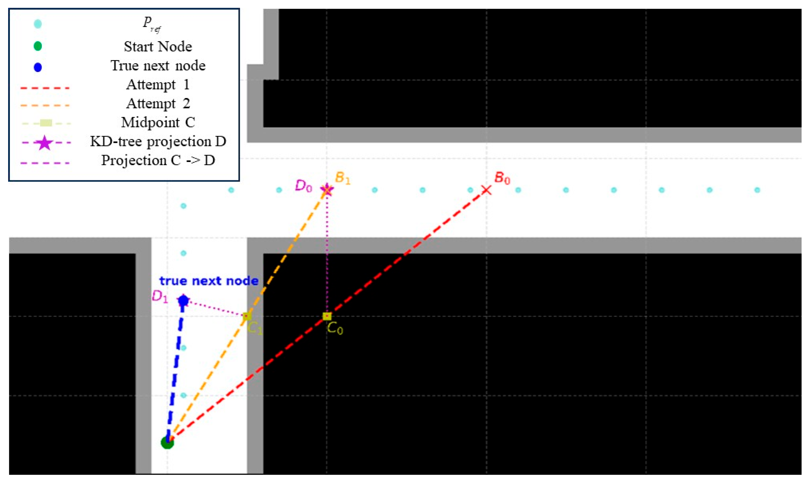
In the upper-layer output processing module, the waypoint sequence P i n i t generated by the upper-layer planner is first densified through linear interpolation to obtain P i n i t . To avoid collisions caused by sparse waypoint sequences, a KD-tree-based fallback mechanism is introduced, as shown in Figure 6 and summarized in Algorithm 2. Specifically, the A*-guided reference path P r e f is organized as a KD-tree for efficient nearest-neighbor search. For each adjacent waypoint pair in P i n i t , the algorithm checks whether the connecting segment intersects the inflated obstacle map. If the segment is collision-free, it is directly interpolated into P i n i t . Otherwise, the midpoint of the invalid segment is computed, and its nearest point in P r e f is selected as the fallback endpoint. This process is repeated, subject to the maximum retry number N r , until the interpolation is completed.
Algorithm 2. Linear interpolation with KD-tree-based Fallback Mechanism
Input: Initial waypoint sequence P i n i t , A*-guided reference path P r e f , Inflated obstacle map M o b s , Maximum retry number N r
Output: Interpolated initial waypoint sequence P i n i t
1: Construct a KD-tree from the A*-guided path P r e f
2: P i n i t = P i n i t
3: for each candidate segment ( p s t a r t , p e n d ) generated from P i n i t  do
4:    r = 0
5:   while ( p s t a r t , p e n d ) collides with M o b s and r < N r  do
6:     p m i d = ( p s t a r t + p e n d ) / 2
7:    Query KD-tree to find the nearest A*-guided point p d to p m i d
8:     p e n d = p d
9:     r = r + 1
10:   end while
11:    p s t a r t = p e n d
12:    P i n i t p e n d
13: end for
return  P i n i t
Based on the discrete spatial coordinates within P i n i t , numerical derivative approximation is then used to estimate the UGV heading angle ψ g k and velocity v g k , as well as the UAV three-axis velocities [ v a x k , v a y k , v a z k ] T and attitude angles ϕ k . By concatenating P i n i t with these supplementary state variables and zero-initialized control inputs, the initial state sequence X i n i t and control sequence U i n i t are constructed as a valid initial guess for the solver.
The NLP solving module then transforms the OCP into a constrained NLP problem using CasADi. The objective function is formulated as
J = w t T + k = 0 N 1 ( w r u g k 2 + w a u a k 2 )
where T = ( k N k 0 ) Δ t is the total planning time, w t is designed to guide the solver toward an optimal trajectory; u g k and u a k denote the UGV and UAV control vectors at step k ; w r and w a regulate the smoothness of the cooperative trajectories. The NLP also includes system transition constraints based on UGV and UAV kinematics in Equations (6) and (7), physical bounds in Equations (9) and (10), safety corridors in Equation (11), two-point boundary value constraints in Equations (4) and (5), and the communication distance constraint in Equation (12).

5.2.2. NLP Resolution via OCDT

In establishing the numerical computation framework for the NLP problem, this paper employs the OCDT [39] (pp. 287–324), also referred to as a simultaneous full-discretization method. Within this framework, the system not only treats the control sequence U = { u g , a 0 , u g , a 1 , , u g , a N 1 } as decision variables but also incorporates the state sequence X = { x g , a 0 , x g , a 1 , , x g , a N 1 } into the optimization variable space. The dimension of the resulting NLP problem can be explicitly determined from the discretized state and control variables. At each discretization node, the UGV state contains 4 variables and the UAV state contains 6 variables, while the UGV and UAV control vectors contain 2 and 6 variables, respectively. Therefore, for an optimization horizon with N control intervals, the full-discretization NLP contains 10(N + 1) state variables and 8N control variables, resulting in a total of 18N + 10 decision variables. In the representative benchmark case used in the experiments, the interpolated trajectory was resampled into N = 120 control intervals, leading to 1210 state variables, 960 control variables, and 2170 decision variables in total.
Compared to partial discretization methods, the OCDT offers an advantage in terms of numerical stability and convergence. Because both state and control variables serve as independent optimization variables at each discrete time step, the continuous system kinematic equations are transcribed into equality constraints between adjacent nodes, denoted as x g , a k + 1 = f ( x g , a k , x g , a k , Δ t ) . This specific structure helps mitigate the trajectory ‘drift’ issue caused by the temporal accumulation of minute perturbations in the initial state, thereby improving the solver with enhanced numerical robustness when tackling highly nonlinear systems. Furthermore, this approach enables the explicit formulation of constraints as algebraic equations with respect to the optimization variables. This structure allows the IPOPT solver to effectively exploit the sparse Jacobian and Hessian matrices of these equations, thereby facilitating efficient computations.

5.2.3. Obstacle-Inflation-Based Safe Corridor Generation

In the OCDT framework, obstacle-inflation-based safety corridors are introduced to handle obstacle avoidance and improve numerical stability in non-convex environments. The UGV and UAV are modeled using a bounding disk and a bounding sphere, respectively. Directly imposing collision-avoidance constraints between these geometric envelopes and obstacles would introduce non-convex Euclidean distance constraints into the NLP problem, increasing computational complexity and potentially affecting convergence. Therefore, the 3D grid map is first inflated according to the maximum robot radius, allowing both agents to be treated as point-mass models. Based on the inflated map, safety corridors are constructed at each discrete node as convex feasible regions represented by linear inequalities. This formulation converts obstacle avoidance into linear boundary constraints and enables IPOPT to exploit the sparse structure of the resulting NLP problem more efficiently. Algorithm 3 summarizes the construction of the obstacle-inflation-based safety corridors.
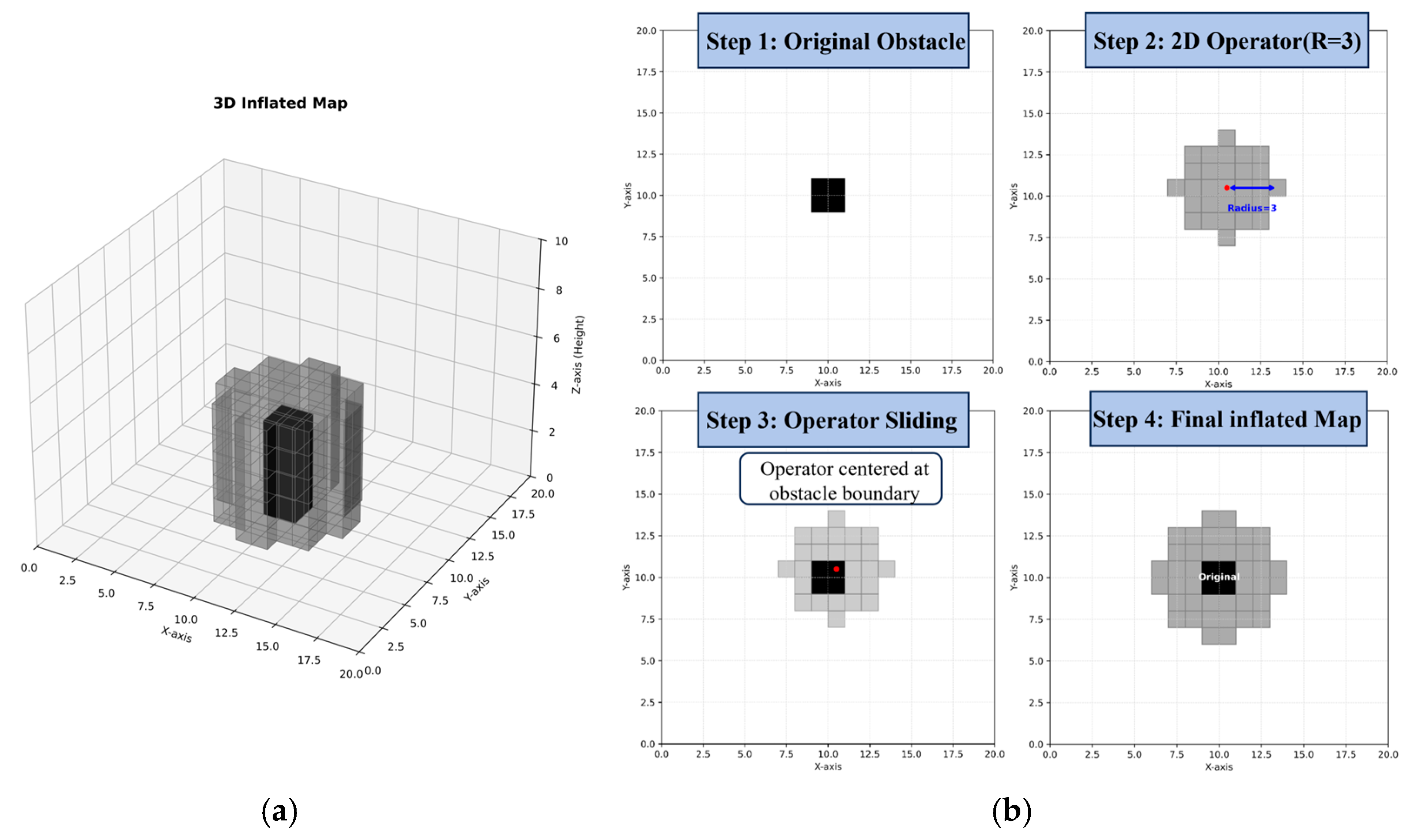
The procedure begins with spatial preprocessing for obstacle inflation. A spatial operator is defined according to the maximum radii of the UGV and UAV. This operator slides over the boundary cells of the original obstacles and marks the covered voxels as occupied, thereby generating M o b s . The inflation process is illustrated in Figure 7.
Based on the inflated map M o b s , the system employs a local bounding box generation algorithm to construct the specific safety corridor constraints. Specifically, centered at the UGV-UAV positional coordinates for each discrete time step k in P i n i t , the algorithm executes an adaptive expansion along the coordinate axes. The expansion logic is implemented as follows: for the UGV, the algorithm probes along four directions Ω u g v = { + x , x , + y , y } , while for the UAV, it performs a six-direction detection Ω u a v = { + x , x , + y , y , + z , z } . During the expansion process, the system monitors the box boundaries in real time to detect any contact with the inflated map. If there is no collision being detected, the expansion in a specific direction will start until a collision is detected or the preset maximum expansion distance L l i m i t is reached. Then, this termination excludes one direction. Adaptive box expansion will stop when all the directions are excluded.
This procedure ultimately generates local box for each waypoint of UGV and UAV, denoted as C k = { Box u g v , k , Box u a v , k } . Ultimately, the final safety corridor is formed by the union of all local boxes generated for each waypoint, denoted as C = { C 0 , , C N } .
Algorithm 3. Safety-Corridor Generation Based on Map Inflation
Input: 3D map M o b s , Unified robot radius r m a x , Initial path P i n i t , Expansion limit L l i m i t
Output: Safety corridors C
1: Step 1: Map Inflation
2: Define Map Element S = { ( i , j , k ) 3 δ i 2 + j 2 + k 2 r m a x }  where  ( i , j , k )  are voxel index offsets relative to any point  p P i n i t  in  M o b s
3: M o b s = max _ filter ( M o b s , S )
4: Step 2: Adaptive Box Expansion and Corridor Generation
5: for each k { 0 , , N }  do
6:    ( x k , y k , z k ) P i n i t
7:   Initialize  Box u g v , k , Box u a v , k ( x k , y k , z k )
8:    For UGV expansion (4 directions):
9:      Ω u g v = { + x , x , + y , y }
10:     while  Ω u g v  do
11:      Expand Box u g v , k along d Ω u g v by Δ s
12:      if  Box u g v , k M o b s  or  dist L l i m i t  then
13:        Ω u g v = Ω u g v \ { d }
14:      end if
15:     end while
16:   For UAV expansion (6 directions):
17:      Ω u a v = { + x , x , + y , y , + z , z }
18:     while  Ω u a v  do
19:       Expand Box u a v , k along d Ω u a v by Δ s
20:       if  Box u a v , k M o b s  or  dist L l i m i t  then
21:        Ω u a v = Ω u a v \ { d }
22:       end if
23:     end while
24:    Construct corridor C k = { Box u g v , k , Box u a v , k }
25: end for
return  C = { C 0 , , C N }

6. Experiments and Results

The proposed hierarchical framework is evaluated in a simulated 3D urban canyon environment constructed from a custom grid map with physical dimensions of 50 m × 50 m and a flight altitude limit of 40 m. The continuous workspace is discretized at a resolution of 0.5 m, resulting in a 100 × 100 × 40 3D grid. Static buildings are represented by a predefined polygonal obstacle dataset. To simplify collision checking and corridor generation, the obstacle map is inflated by an equivalent physical radius of 1.5 m, allowing the UGV and UAV to be treated as point-mass models in the subsequent NLP optimization. The algorithms are implemented in Python 3.10, with the DRL module developed using PyTorch 2.10.0 and the NLP problem solved by CasADi with the IPOPT solver. All simulations are conducted on a laptop equipped with an Intel(R) Core (TM) Ultra 9 275HX @ 2.70 GHz processor, 32 GB RAM, and an NVIDIA GeForce RTX 5070 Laptop GPU. The main simulation and planning parameters are summarized in Table 2.

6.1. Visualization of Planning Results

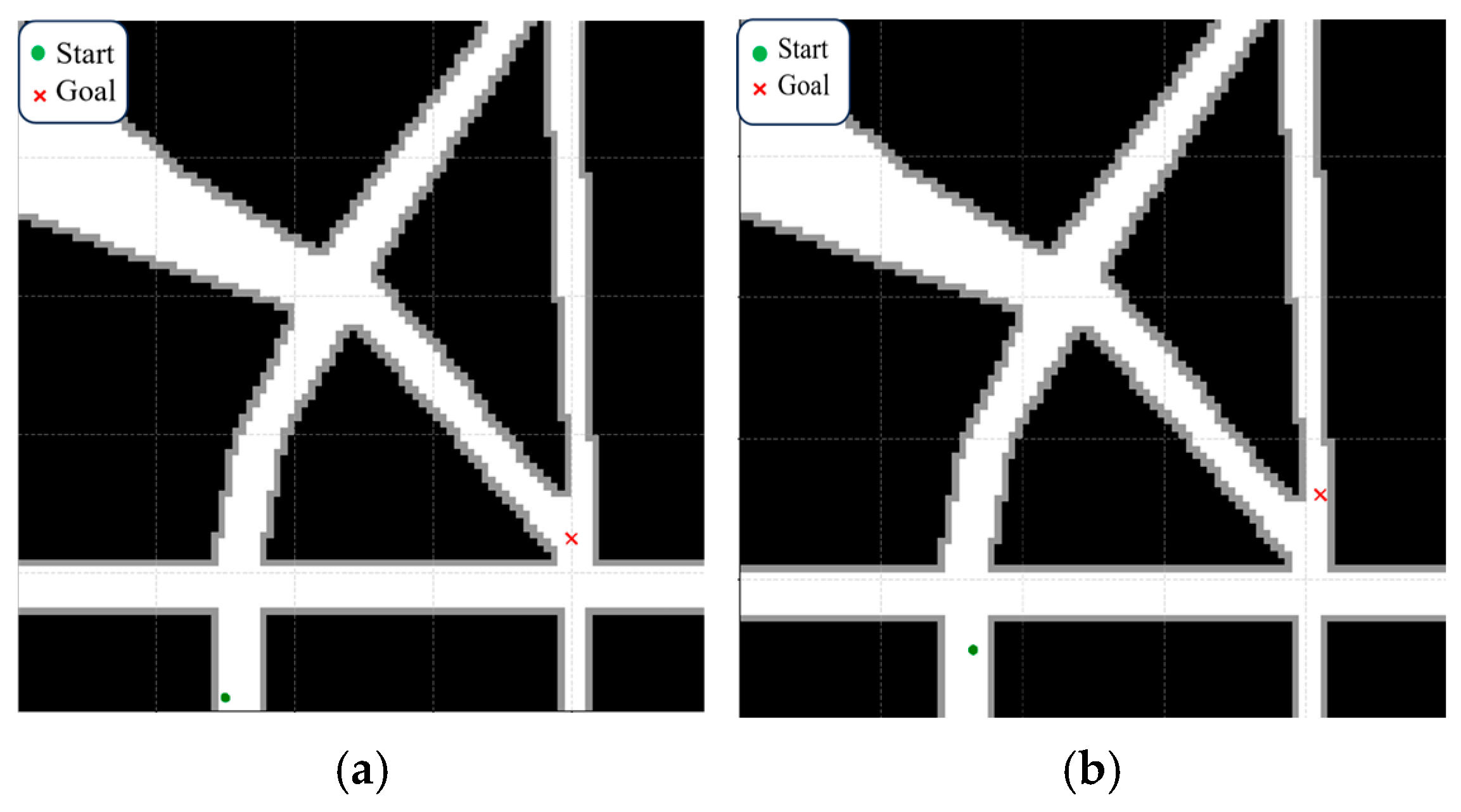
This Section details the operational pipeline of our proposed framework and presents both the final cooperative trajectories and the intermediate results at each stage. Given that 3D visualizations often fail to provide a clear perspective of the results, all figures—with the exception of the final cooperative trajectory plots, which include partial 3D views—are presented as 2D projections of the 3D scene onto the XY plane. Regarding the planning task setup, it is assumed that the UAV has already detached from the UGV at the starting position and is hovering at its minimum safe flight altitude directly above the UGV. Furthermore, the UGV is designated as the primary planning-task executor, while the UAV serves solely for communication support. Consequently, once the UGV reaches the goal, the UAV will hover at a specific distance from the UGV, with the assumption that it can autonomously navigate back to the destination of the UGV upon task completion. To examine planner performance, two distinct sets of start and goal positions are evaluated, as illustrated in Figure 8.
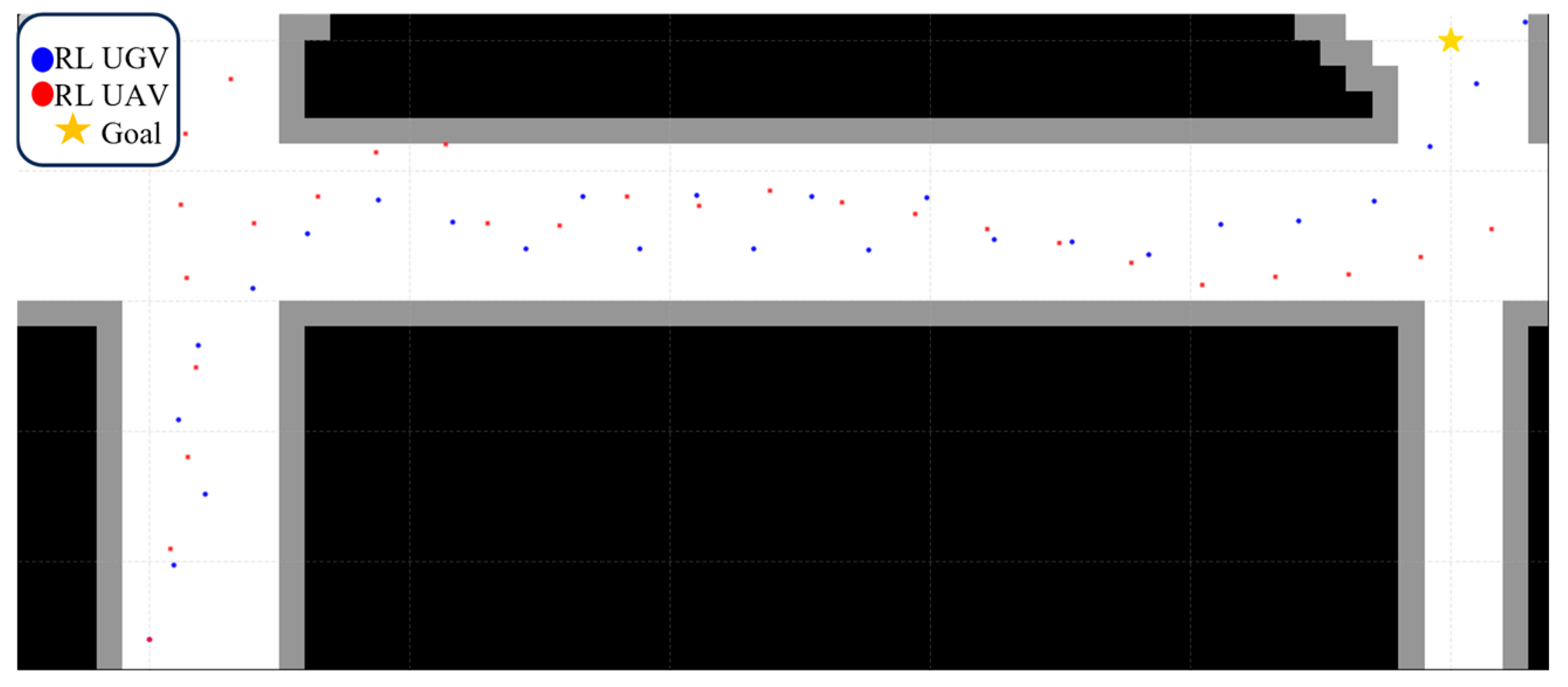
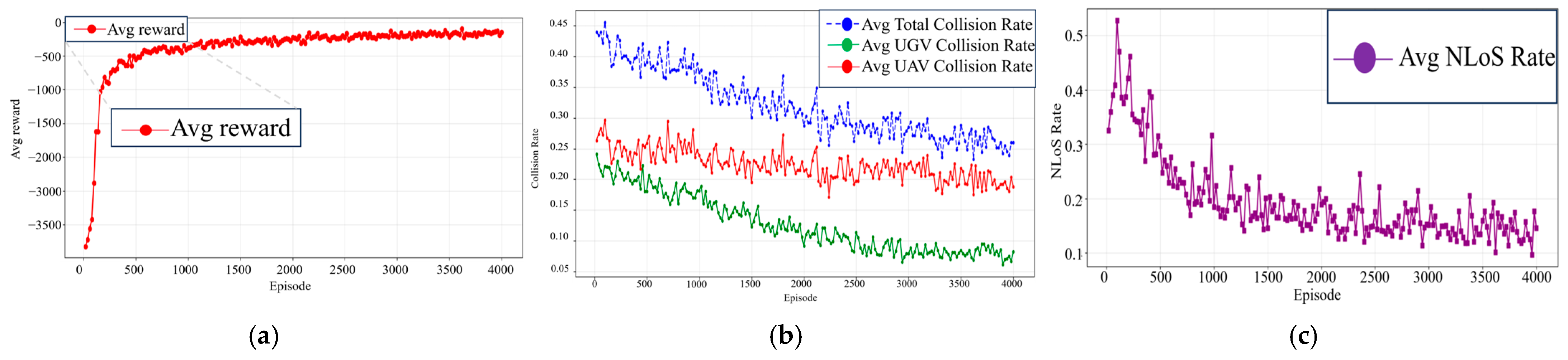
Initially, the start and goal positions illustrated in Figure 8a are fed into the upper-layer planner. Guided by a sampling-based A* path, the RL algorithm derives the initial set of waypoints P i n i t for the UGV-UAV system, as depicted in Figure 9. The DRL agent was trained for 4000 episodes. In our evaluation, the collision rate is defined as the ratio of the total collision occurrences to the aggregate number of steps within a single episode. The training results, as displayed in Figure 10, show a stable convergence trend of the reward function. Specifically, the initial paths generated by the RL agent exhibit an overall collision rate of 11.89%—comprising approximately 5–10% for the UGV and 20% for the UAV—along with an average NLoS communication rate of nearly 15%. To improve reproducibility, the detailed hyperparameters used for PPO training are summarized in Table 3.
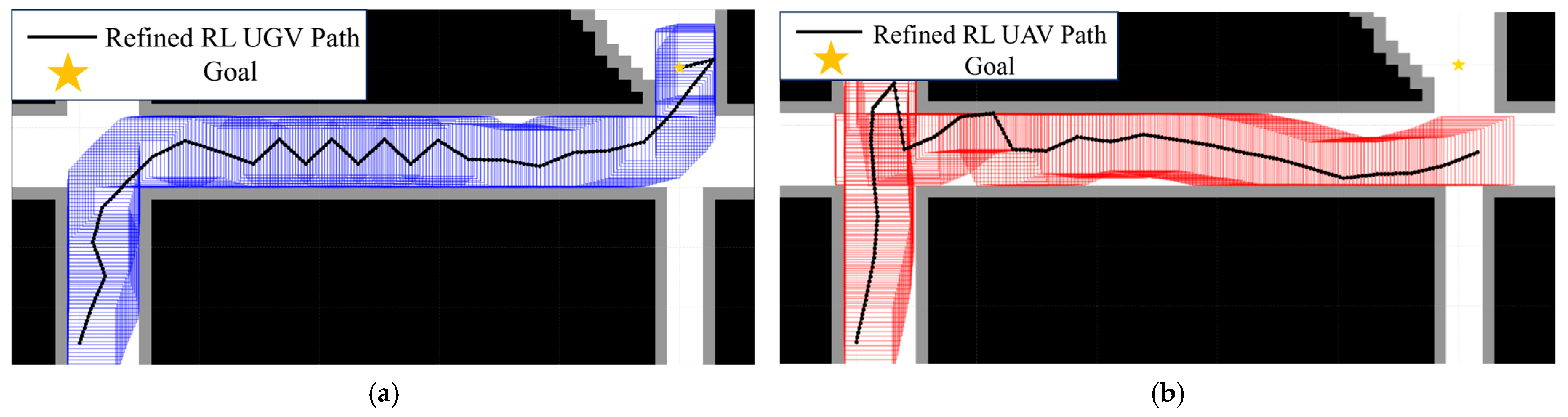
Subsequently, we apply a linear interpolation process integrated with a back-off strategy to the initial waypoints P i n i t produced by the upper-layer planner. By interpolating 10 intermediate points between each pair of adjacent waypoints, we construct the refined initial solution P i n i t , which serves as the input for the lower-layer numerical solver. Then, an obstacle-inflation-based corridor construction algorithm is applied to each initial solution to generate the respective safety corridors for the UGV and the UAV, as illustrated in Figure 11.
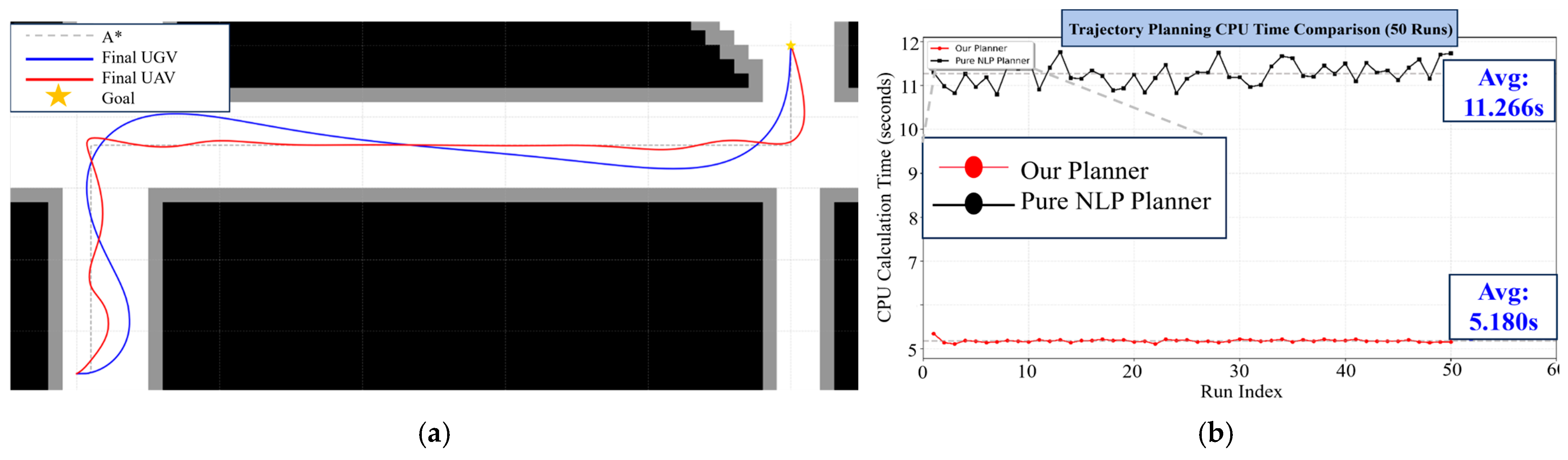
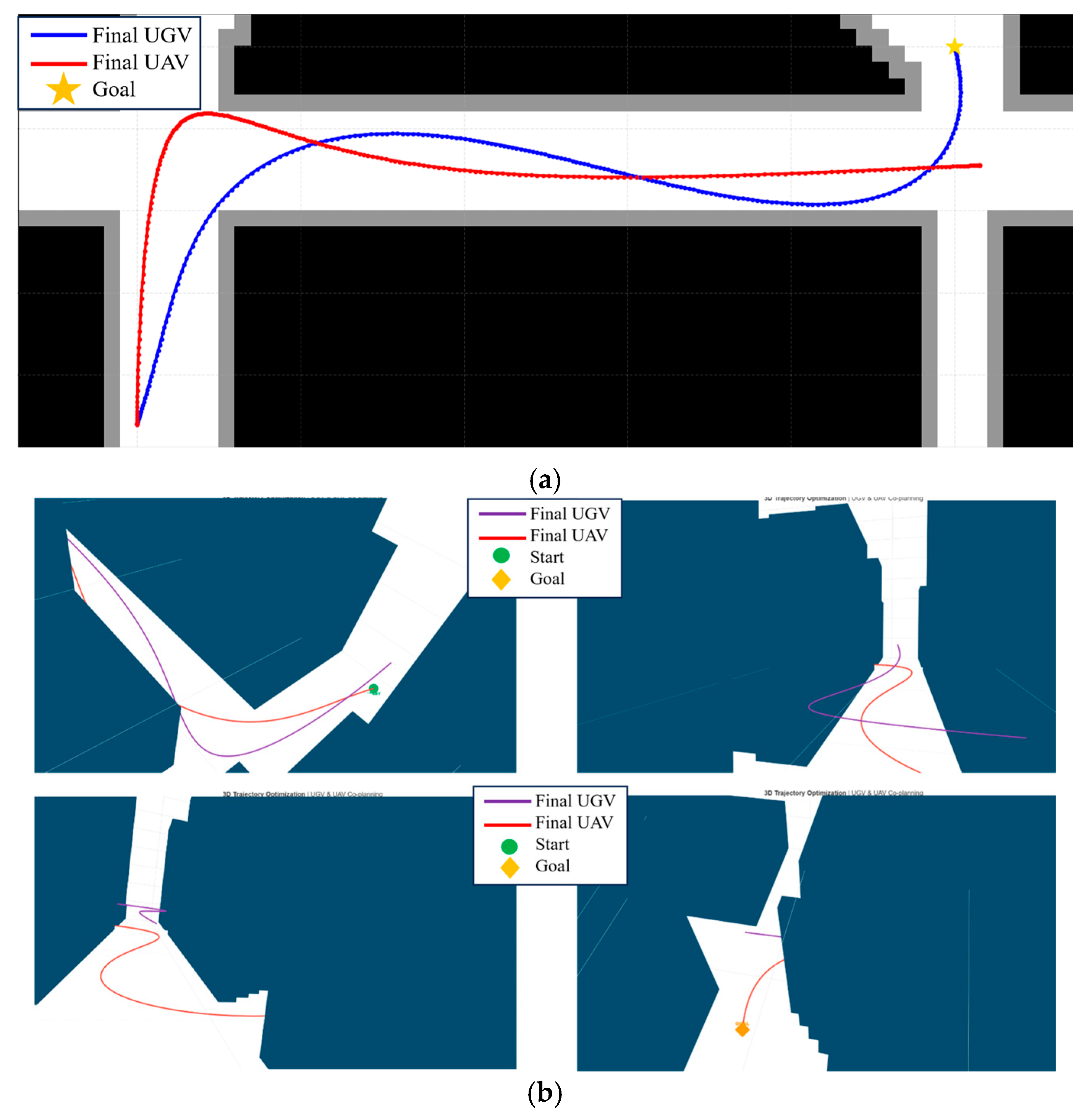
Finally, based on P i n i t , we initialize the remaining state initial sequence X and the control initial sequence U . These sequences, along with the safety corridor constraints, system-level constraints, and the objective function, are fed into the IPOPT solver. This numerical optimization process yields the final cooperative trajectory output, as presented in Figure 12.
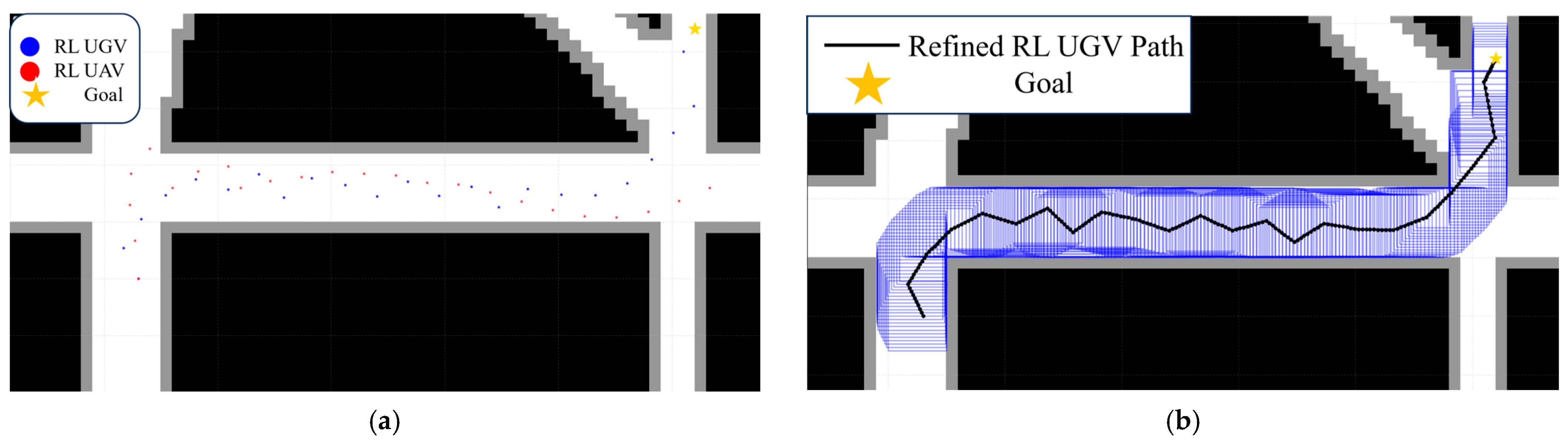
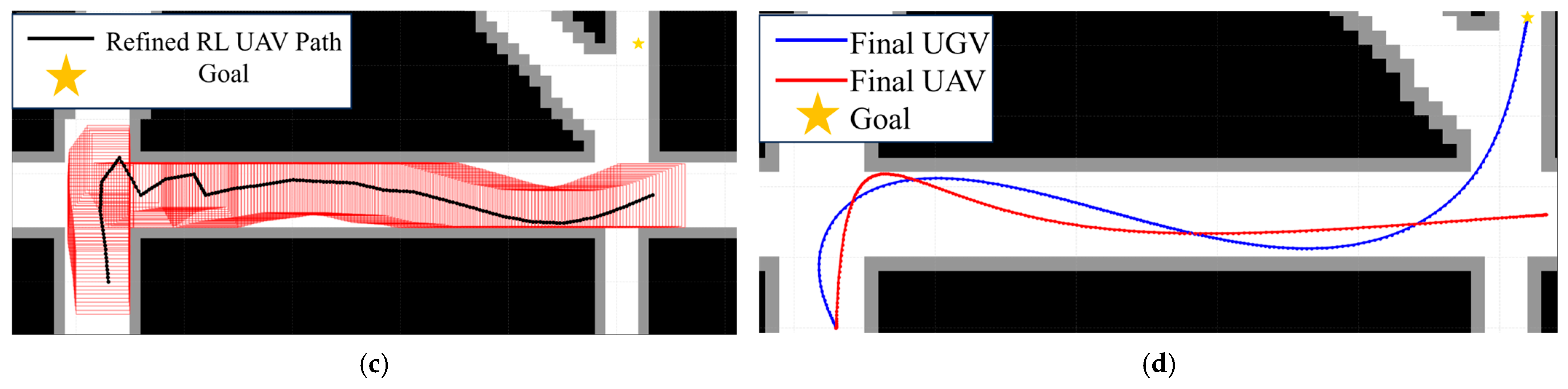
To further examine the planning performance of the proposed hierarchical framework under a different start-goal configuration within the same simulated urban canyon environment, we conducted an additional evaluation based on the scenario shown in Figure 8b. In this test, the initial RL-generated paths exhibit a collision rate of 16.7% and an average NLoS communication rate of 17%. After being processed by the lower-layer optimization module with corridor-based constraints, the final cooperative UGV-UAV trajectories become smooth, collision-free, and communication-aware, as shown in Figure 13. These results indicate that the proposed hierarchical framework can improve the quality and feasibility of initial trajectories in the tested simulated urban canyon scenario.
The above experiments were conducted at the trajectory planning level in simulated urban canyon scenarios. The proposed framework is designed as a scenario-specific deployment approach rather than a map-agnostic reinforcement learning method. In practical deployment, the urban map is assumed to be known in advance, and the obstacle map, communication visibility structure, A*-based guidance paths, and RL state representation are constructed according to the given scenario. If the deployment environment changes, the map construction module needs to rebuild the obstacle and communication maps, and the A*-guided RL module should be retrained offline using the updated environmental information before online trajectory refinement is performed by the lower-layer optimizer. Therefore, the current experiments should be interpreted as planning-level validation in the tested urban canyon scenarios, rather than as evidence of zero-shot generalization across arbitrary unseen maps or full real-world system robustness.

6.2. Ablation and Comparison Experiments

This Section provides a systematic evaluation of the role of the proposed algorithm through multi-dimensional testing. First, ablation studies are conducted to assess the contribution of each module; subsequently, comparative experiments are presented to compare its performance with representative baseline methods. All these experiments are based on the set of start and end points in Figure 8a.

6.2.1. Ablation Experiments

To evaluate the role of the upper-layer RL module, ablation experiment 1 removes RL and directly uses the discrete path generated by the A* algorithm as the initial guess for the NLP solver. To define the cooperative terminal state, the UAV target node is aligned with the UGV destination. The CPU execution time of this A*-guided NLP-only planner is compared with that of the full hierarchical framework over 50 independent trials. As shown in Figure 14, the NLP-only planner can generate feasible cooperative trajectories, but it requires a longer and less stable solving process. The proposed framework achieves an average planning time of 5.180 s, whereas the NLP-only planner requires 11.266 s on average, with larger temporal fluctuations.
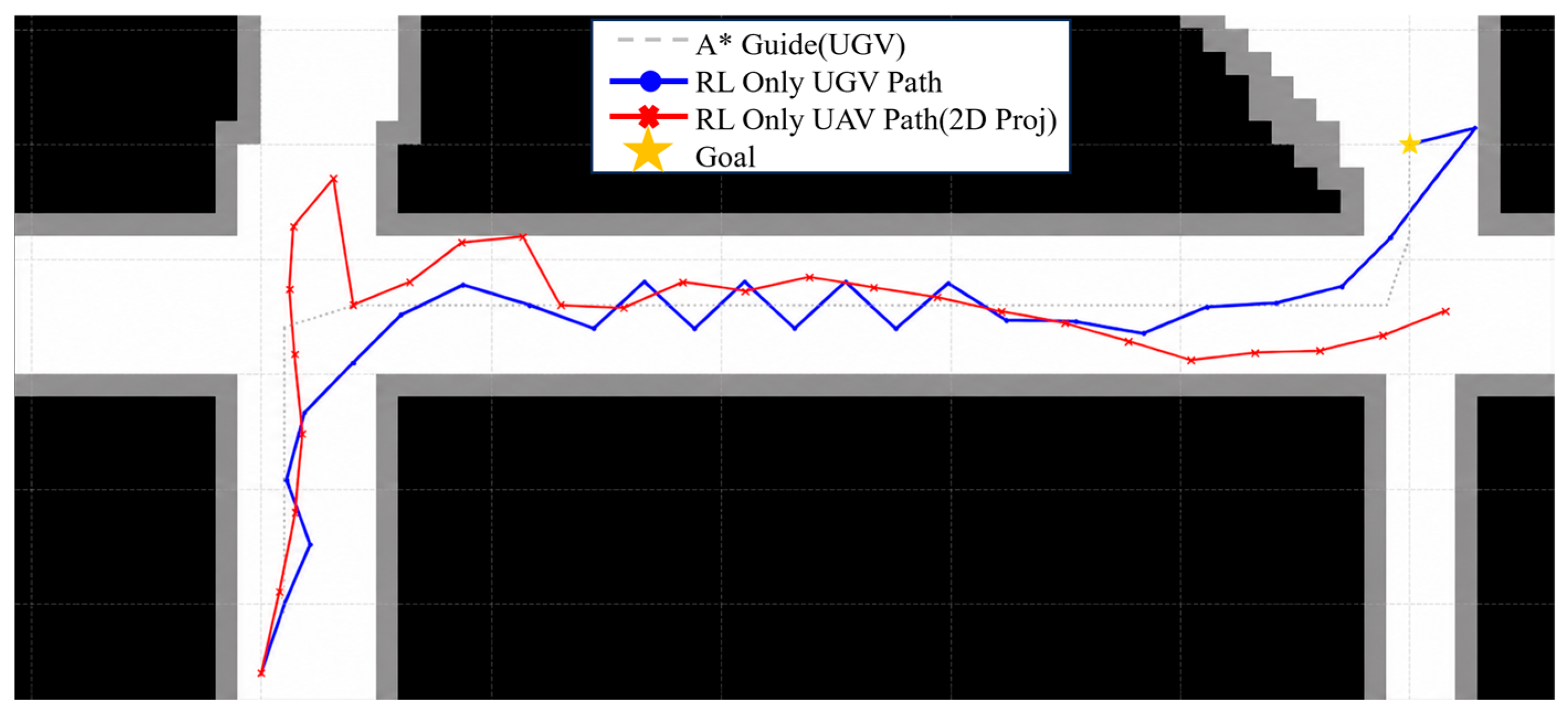
To examine the role of the lower-layer NLP solver, ablation experiment 2 removes the optimization phase and directly uses the DRL output as the cooperative trajectory. As shown in Figure 15, the pure RL planner can guide the UGV-UAV system toward the goal at the topological level, but the resulting trajectories are discrete and less smooth. The UGV and UAV paths exhibit step-like jumps and oscillations due to the sampled action outputs of the neural policy. Quantitatively, the pure RL strategy produces three collisions, including one UGV collision, two UAV collisions, and three NLoS events within a 26-step horizon.
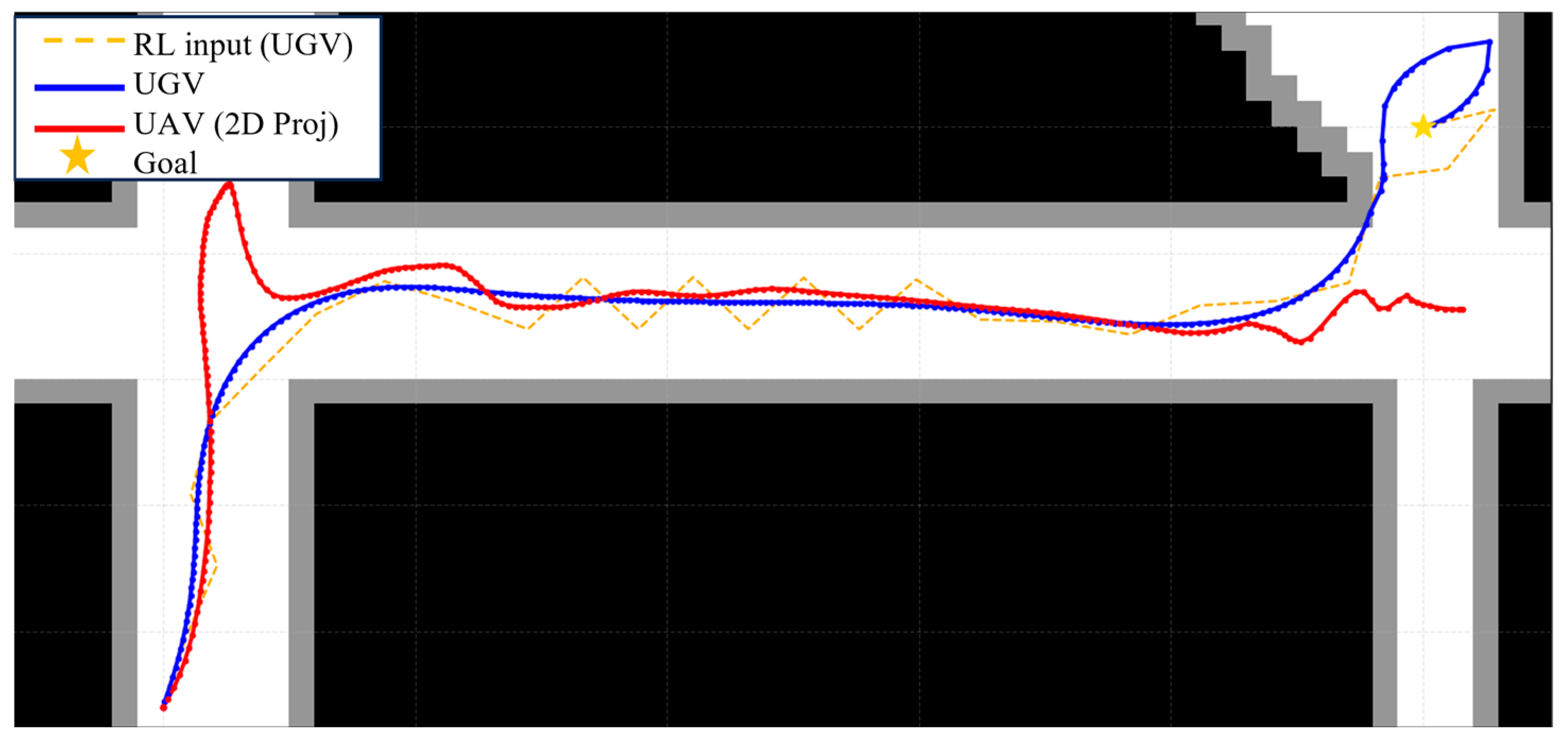
To assess the intermediate waypoint-processing mechanism, ablation experiment 3 removes the KD-tree-based back-off logic and directly feeds the linearly interpolated RL waypoints into the lower-layer NLP solver. The resulting trajectory is shown in Figure 16.
Without the back-off correction, part of the interpolated UGV initial guess penetrates the inflated obstacles. As a result, the local corridor generation process produces infeasible or near-zero-volume safety regions around these invalid waypoints. These infeasible corridor constraints cause conflicts between equality and inequality constraints in the NLP formulation, leading to solver failure and distorted trajectories that intersect the inflated obstacles.
Overall, the ablation results indicate that the three components play complementary roles in the proposed framework. The upper-layer RL module provides a structured and communication-aware initial guess, reducing the computational burden of the NLP solver. The lower-layer NLP solver improves trajectory smoothness and enforces hard kinematic, collision-avoidance, and communication constraints. The intermediate waypoint-processing mechanism further improves the feasibility of the initial guess and supports reliable safety-corridor generation. Together, these modules contribute to the efficiency, feasibility, and robustness of the proposed hierarchical planner.

6.2.2. Comparison Experiment

To further evaluate the proposed hierarchical cooperative planner, we compare the Layered Planner with three representative baselines. The first baseline is sdSCA, which represents population-based meta-heuristic optimization [40]. The second baseline is RB-PPO, adapted from the multi-UAV path-planning method in [41]. The original RB-PPO improves PPO by using a replay buffer and a rollback-based objective for more stable policy updates. In this paper, it is adapted to the UGV-UAV relay task by replacing the original homogeneous multi-UAV state, action, and reward definitions with the proposed air–ground state representation, UGV/UAV displacement actions, and rewards related to goal progress, obstacle avoidance, NLoS penalty, and communication range. The trained policy directly outputs synchronized UGV-UAV trajectories without lower-layer NLP refinement. The third baseline is RRT*-NLP, adapted from the random-sampling and nonlinear-optimization framework in [42]. The original method first uses RRT* to generate a single-vehicle reference path and then applies nonlinear optimization to improve trajectory smoothness and constraint satisfaction. In this paper, RRT* is used to generate the UGV topological route, while the UAV relay waypoints are initialized according to the UGV route and communication constraints. The resulting cooperative initial trajectory is then refined by NLP under the same obstacle, NLoS, communication range, and heterogeneous kinematic constraints.
For stochastic baselines, including sdSCA and RRT*-NLP, 50 independent trials with different random seeds are conducted, and the results are reported as mean ± standard deviation in Table 4. The proposed Layered Planner and RB-PPO are evaluated under a fixed trained policy, map, and start-goal pair, so single-run values are reported. Solver success rate is included to assess numerical robustness; for methods without an explicit NLP solver, it indicates whether a valid trajectory is generated.
The proposed Layered Planner achieves 0.0% UGV collision rate, 0.0% UAV collision rate, 0.0% NLoS rate, and the lowest UGV/UAV smoothness values of 0.0157 and 0.0165, respectively. Its total runtime is 6.172 s, including map and communication-visibility construction/update, 0.32 s; A*-based guidance path generation, 0.41 s; upper-layer RL inference, 0.48 s; waypoint interpolation and safe-corridor generation, 0.74 s; NLP transcription and CasADi model construction, 0.56 s; and IPOPT numerical optimization, 3.66 s.
This shows that NLP optimization is the main computational component, while the upper-layer guidance reduces the NLP search burden by providing a structured warm start. Compared with the proposed method, sdSCA has much higher UGV collision and NLoS rates, 24.8 ± 15.5% and 48.0 ± 10.1%, respectively, and a longer runtime of 220.471 ± 75.693 s. RB-PPO is the fastest method, requiring only 0.594 s, but it still produces UGV and UAV collision rates of 3.8% and 7.7%, indicating that learning-based planning alone may not strictly enforce hard feasibility constraints. RRT*-NLP achieves low collision and NLoS rates, but its smoothness, runtime, and solver success rate are still inferior to those of the proposed Layered Planner.
Statistical significance is further assessed by comparing each stochastic baseline with the proposed Layered Planner. A one-sample Wilcoxon signed-rank test with Holm–Bonferroni correction is used, and the significance levels are denoted as * for p < 0.05, ** for p < 0.01, and *** for p < 0.001. As shown in Table 5, the proposed method significantly outperforms sdSCA in UGV collision rate, NLoS rate, UGV/UAV smoothness, and computational time. Compared with RRT*-NLP, it shows significant improvements in NLoS rate, UGV/UAV smoothness, and computational time. These results indicate that the Layered Planner achieves a better balance among topological guidance, constraint satisfaction, trajectory smoothness, computational efficiency, and solver robustness.

7. Discussion

The proposed hierarchical framework is useful, as supported by our ablation studies. First, when the RL-guided upper layer is removed, the NLP solver can still generate feasible trajectories in some cases, but it becomes more computationally expensive and more sensitive to local minima, indicating that a structured initial solution is important for handling the highly non-convex cooperative planning problem. Second, when the lower-layer NLP refinement is removed, the raw RL output remains discrete, less smooth, and does not by itself strictly guarantee kinematic feasibility, collision avoidance, and communication satisfaction. Third, removing the intermediate waypoint-processing mechanism can lead to infeasible initial guesses and less reliable corridor generation, which may further affect solver convergence.
Nevertheless, the current study still has several limitations. Several open research questions and future directions arise from the current study. First, the communication model is based on a binary NLoS indicator. However, this simplified representation does not capture more realistic physical-layer effects, such as distance-dependent path loss, multipath fading, interference, or dynamic blockage. Future work will therefore investigate how to integrate more realistic physical-layer communication models into trajectory optimization. Second, experimental validation is currently restricted to simulated urban canyon scenarios. More specifically, the present evaluation still relies entirely on simplified grid-based simulations, without higher-fidelity simulation environments or real-world validation. Although these simulations provide useful insights into planning-level performance, high-fidelity simulations and real-world UGV-UAV experiments are still needed to further assess practical deployment performance and validate the robustness of the proposed framework.

8. Conclusions

This paper proposed a hierarchical cooperative trajectory planning framework for UGV-UAV systems in communication-constrained urban canyon environments. The framework uses A*-guided RL to generate structured cooperative waypoints and employs corridor-constrained NLP to refine them into feasible and smooth trajectories.
Simulation results show that the proposed framework can generate collision-free, communication-aware, and smooth cooperative trajectories in the tested urban canyon scenarios. Ablation and comparison experiments further indicate its advantages in trajectory feasibility, communication reliability, computational efficiency, and solver success rate over representative baseline methods.

Author Contributions

Conceptualization and writing—review and editing, F.B.; investigation, methodology, validation and writing—original draft preparation, D.G.; resources and funding acquisition, Y.Z.; data curation and visualization, H.N. All authors have read and agreed to the published version of the manuscript.

Funding

This research was funded by the 2024 Beijing Natural Science Foundation–Xiaomi Joint Innovation Fund, grant number L243024. The APC was funded by the Beijing Natural Science Foundation-Xiaomi Joint Innovation Fund and the authors.

Data Availability Statement

The original contributions presented in this study are included in the article. Further inquiries can be directed to the corresponding author.

Acknowledgments

During the revision and preparation of this manuscript, the authors used generative AI tools, including ChatGPT5.5, to assist with language polishing, grammatical correction, structural refinement, and improvement of clarity in the literature review, discussion, and response-to-reviewer materials. Generative AI tools were not used to generate original research ideas, mathematical models, simulation data, experimental results, figures, or references. The authors carefully reviewed and edited all AI-assisted outputs and take full responsibility for the content, accuracy, originality, and integrity of the final manuscript.

Conflicts of Interest

The authors declare no conflicts of interest.

References

  1. Nie, L.; Zhang, T.; Zhao, Y.; Li, Y.; Li, H.; Yang, J. Distributed Multi-Vehicle Cooperative Trajectory Planning and Control for Ramp Merging and Diverging Based on Deep Neural Networks and MPC. Machines 2026, 14, 262. [Google Scholar] [CrossRef]
  2. Balaska, V.; Tsiakas, K.; Giakoumis, D.; Kostavelis, I.; Folinas, D.; Gasteratos, A.; Tzovaras, D. A Viewpoint on the Challenges and Solutions for Driverless Last-Mile Delivery. Machines 2022, 10, 1059. [Google Scholar] [CrossRef]
  3. Quero, C.O.; Martinez-Carranza, J. Unmanned aerial systems in search and rescue: A global perspective on current challenges and future applications. Int. J. Disaster Risk Reduct. 2025, 118, 105199. [Google Scholar] [CrossRef]
  4. Wandelt, S.; Wang, S.; Zheng, C.; Sun, X. AERIAL: A Meta Review and Discussion of Challenges Toward Unmanned Aerial Vehicle Operations in Logistics, Mobility, and Monitoring. IEEE Trans. Intell. Transp. Syst. 2024, 25, 6276–6289. [Google Scholar] [CrossRef]
  5. Franceschetti, G.; Iodice, A.; Riccio, D. Radio Propagation in the Urban Scenario; Artech House: Norwood, MA, USA, 2023. [Google Scholar]
  6. Browning, J.W.; Cotton, S.L.; Sofotasios, P.C.; Morales-Jimenez, D.; Yacoub, M.D. A Unification of LoS, Non-LoS, and Quasi-LoS Signal Propagation in Wireless Channels. IEEE Trans. Antennas Propag. 2023, 71, 2682–2696. [Google Scholar] [CrossRef]
  7. Rappaport, T.S. Wireless Communications: Principles and Practice, 2nd ed.; Cambridge University Press: Cambridge, UK, 2024. [Google Scholar] [CrossRef]
  8. Meng, X.; Zhang, Z.; Zhu, X.; Zhao, J.; Wu, X.; Zhang, X.; Yang, J. Obstacle Avoidance Path Planning for Unmanned Aerial Vehicle in Workshops Based on Parameter-Optimized Artificial Potential Field A* Algorithm. Machines 2025, 13, 967. [Google Scholar] [CrossRef]
  9. Qiao, L.; Luo, X.; Luo, Q. Control of Trajectory Tracking for Mobile Manipulator Robot with Kinematic Limitations and Self-Collision Avoidance. Machines 2022, 10, 1232. [Google Scholar] [CrossRef]
  10. Bao, Z.; Zhang, Z.; Xie, C. Landmark selection and path planning for unmanned vehicles with position error corrections. Transp. Res. Part C Emerg. Technol. 2023, 153, 104186. [Google Scholar] [CrossRef]
  11. Chen, X.; Qin, G.; Sun, J. Coordinated routing policy for connected vehicles to monitor city-wide traffic. Transp. Res. Part C Emerg. Technol. 2025, 176, 105147. [Google Scholar] [CrossRef]
  12. Wu, Y.; Low, K.H.; Hu, X. Trajectory-based flight scheduling for AirMetro in urban environments by conflict resolution. Transp. Res. Part C Emerg. Technol. 2021, 131, 103355. [Google Scholar] [CrossRef]
  13. Ayalew, M.; Zhou, S.; Memon, I.; Heyat, M.B.B.; Akhtar, F.; Zhang, X. View-Invariant Spatiotemporal Attentive Motion Planning and Control Network for Autonomous Vehicles. Machines 2022, 10, 1193. [Google Scholar] [CrossRef]
  14. Du, W.; Guo, T.; Chen, J.; Li, B.; Zhu, G.; Cao, X. Cooperative pursuit of unauthorized UAVs in urban airspace via Multi-agent reinforcement learning. Transp. Res. Part C Emerg. Technol. 2021, 128, 103122. [Google Scholar] [CrossRef]
  15. Xia, H.; Zhang, M.; Ma, Z.; Cui, M.; Yan, C. Optimization of Urban Emergency Multimodal Transportation Scheduling with UAV-Ground Traffic Coordination. IEEE Trans. Intell. Transp. Syst. 2026, 27, 692–708. [Google Scholar] [CrossRef]
  16. Wang, C.; Wang, J.; Ma, Z.; Xu, M.; Qi, K.; Ji, Z.; Wei, C. Integrated Learning-Based Framework for Autonomous Quadrotor UAV Landing on a Collaborative Moving UGV. IEEE Trans. Veh. Technol. 2024, 73, 16092–16107. [Google Scholar] [CrossRef]
  17. Zeng, F.; Chen, Z.; Clarke, J.-P.; Goldsman, D. Nested vehicle routing problem: Optimizing drone-truck surveillance operations. Transp. Res. Part C Emerg. Technol. 2022, 139, 103645. [Google Scholar] [CrossRef]
  18. Park, J.; Choi, S.; Kim, T.; Lee, C.; Lee, S. Public Bus-Assisted Task Offloading for UAVs. IEEE Trans. Intell. Transp. Syst. 2024, 25, 20561–20573. [Google Scholar] [CrossRef]
  19. Qin, P.; Wang, Y.; Zhang, J.; Li, P.; Fu, Y. Multi-Type Disaster Scenario Task Offloading in Air–Ground Integrated Search and Rescue Networks: A Blockchain-Assisted MFL Approach. IEEE Trans. Veh. Technol. 2025, 74, 19583–19597. [Google Scholar] [CrossRef]
  20. Xie, R.; Meng, Z.; Wang, L.; Li, H.; Wang, K.; Wu, Z. Unmanned Aerial Vehicle Path Planning Algorithm Based on Deep Reinforcement Learning in Large-Scale and Dynamic Environments. IEEE Access 2021, 9, 24884–24900. [Google Scholar] [CrossRef]
  21. Oubbati, O.S.; Alotaibi, J.; Alromithy, F.; Atiquzzaman, M.; Altimania, M.R. A UAV-UGV Cooperative System: Patrolling and Energy Management for Urban Monitoring. IEEE Trans. Veh. Technol. 2025, 74, 13521–13536. [Google Scholar] [CrossRef]
  22. Sun, L.; Wan, L.; Wang, J.; Lin, L.; Gen, M. Joint Resource Scheduling for UAV-Enabled Mobile Edge Computing System in Internet of Vehicles. IEEE Trans. Intell. Transp. Syst. 2023, 24, 15624–15632. [Google Scholar] [CrossRef]
  23. Jang, G.; Lee, K. Joint Optimization of Path Planning and Cooperative Strategy for UAV–UGV Delivery. IEEE Trans. Intell. Transp. Syst. 2025, 26, 20176–20186. [Google Scholar] [CrossRef]
  24. Li, K.; Cui, H.; Meng, Q.; Zhang, X. Dynamic truck-drone collaborative transportation during hurricanes. Transp. Res. Part C Emerg. Technol. 2025, 180, 105322. [Google Scholar] [CrossRef]
  25. Yoon, S.; Lee, K. Optimal Load Balancing of Cooperative UAV-UGV Parcel Pickup to Minimize Completion Time. IEEE Trans. Intell. Transp. Syst. 2025, 26, 12712–12718. [Google Scholar] [CrossRef]
  26. Li, Y.; Wang, S.; Sun, H.; Zhou, S. Collaborative vessel–unmanned aerial vehicle routing for time-window-constrained offshore parcel delivery. Transp. Res. Part C Emerg. Technol. 2025, 178, 105189. [Google Scholar] [CrossRef]
  27. Ma, Z.; Xiong, J.; Gong, H.; Wang, X. Adaptive Depth Graph Neural Network-Based Dynamic Task Allocation for UAV-UGVs Under Complex Environments. IEEE Trans. Intell. Veh. 2025, 10, 3573–3586. [Google Scholar] [CrossRef]
  28. Zhu, B.; Zheng, Y.; Wang, M.; Ge, Q.; Huang, Y. IMM-AIS-UKF: A GAN-Enhanced Dynamics-Constrained Trajectory Predictor with DDPG Method for UAV-USV Interaction. IEEE Trans. Intell. Transp. Syst. 2025. [Google Scholar] [CrossRef]
  29. Tian, L.; Wang, X.; Chen, H. Heterogeneous Formation Tracking for Fixed-Wing UAVs and Nonholonomic UGVs with Different Asymmetric Constraints. IEEE Trans. Veh. Technol. 2025, 74, 13350–13360. [Google Scholar] [CrossRef]
  30. Yan, Y.; Liang, H.; Cheng, Y.; Li, T. Robust Distributed Formation Control for Heterogeneous UAVs–UGVs Systems: An Adaptive Asymptotic Funnel Control Approach. IEEE Trans. Veh. Technol. 2025, 74, 15619–15630. [Google Scholar] [CrossRef]
  31. Liang, H.; Yang, S.; Li, T.; Zhang, H. Distributed Adaptive Cooperative Control for Human-in-the-Loop Heterogeneous UAV-UGV Systems with Prescribed Performance. IEEE Trans. Intell. Veh. 2024, 9, 6912–6925. [Google Scholar] [CrossRef]
  32. Cosenza, C.; Malfi, P.; Melluso, F.; Nicolella, A.; Niola, V.; Savino, S.; Spirto, M.; Tordela, C. A Virtual Sensor for Wheel Angular Speed Estimation: Application on a Differential Drive Wheeled Robot. J. Intell. Robot. Syst. 2025, 111, 117. [Google Scholar] [CrossRef]
  33. Zhao, X.; Tang, P.; Song, Q.; Jiang, T.; Wang, Y.; Tian, L.; Li, W.; Zhang, J. Experimental Analysis of Multipath Effects on GNSS Positioning in Urban Canyon. In Proceedings of the 2021 IEEE 4th International Conference on Electronic Information and Communication Technology (ICEICT), Xi’an, China, 14–16 May 2021; pp. 557–562. [Google Scholar] [CrossRef]
  34. Liu, X.; Wen, W.W.; Huang, F.; Gao, H.; Wang, Y.; Hsu, L. 3-D LiDAR-Aided GNSS NLOS Mitigation for Reliable GNSS-RTK Positioning in Urban Canyons. IEEE Trans. Instrum. Meas. 2025, 74, 1–15. [Google Scholar] [CrossRef]
  35. Zhong, Y.; Wen, W.; Hsu, L.-T. Trajectory Smoothing Using GNSS/PDR Integration via Factor Graph Optimization in Urban Canyons. IEEE Internet Things J. 2024, 11, 25425–25439. [Google Scholar] [CrossRef]
  36. Ni, H.; Chen, P.; Yu, G.; Chen, Z. Collaborative trajectory planning for CAVs at unstructured intersections considering departure time windows and terrain features. IEEE Trans. Veh. Technol. 2026. [Google Scholar] [CrossRef]
  37. Liao, Y.; Yu, G.; Chen, P.; Zhou, B.; Li, H. Integration of Decision-Making and Motion Planning for Autonomous Driving Based on Double-Layer Reinforcement Learning Framework. IEEE Trans. Veh. Technol. 2024, 73, 3142–3158. [Google Scholar] [CrossRef]
  38. Huang, L.; Chai, R.; Chen, K.; Zhang, J.; Chai, S.; Xia, Y. Navigating Partially Unknown Environments: A Weakly Supervised Learning Approach to Path Planning. IEEE Trans. Intell. Veh. 2024, 9, 7084–7096. [Google Scholar] [CrossRef]
  39. Biegler, L.T. Nonlinear Programming: Concepts, Algorithms, and Applications to Chemical Processes; Society for Industrial and Applied Mathematics: Philadelphia, PA, USA, 2010; pp. 287–324. [Google Scholar] [CrossRef]
  40. Akay, R.; Yildirim, M.Y. Multi-strategy and self-adaptive differential sine–cosine algorithm for multi-robot path planning. Expert Syst. Appl. 2023, 232, 120849. [Google Scholar] [CrossRef]
  41. Zhu, W.; Fang, W.; Su, Y. Path Planning for Multi-UAV Based on Improved Proximal Policy Optimization Algorithm. In Proceedings of the 2024 39th Youth Academic Annual Conference of Chinese Association of Automation (YAC), Dalian, China, 7–9 June 2024; pp. 1890–1894. [Google Scholar] [CrossRef]
  42. Wang, J.; Li, J.; Yang, J.; Meng, X.; Fu, T. Automatic Parking Trajectory Planning Based on Random Sampling and Nonlinear Optimization. J. Frankl. Inst. 2023, 360, 9579–9601. [Google Scholar] [CrossRef]
Figure 1. Communication-constrained UGV-UAV relay scenario in an urban canyon. The UAV restores connectivity when high-rise buildings block the direct LoS link between the UGV and external infrastructure.
Machines 14 00594 g001
Figure 2. Kinematic model for UGV and UAV: (a) the UGV is described by a kinematic bicycle model; (b) the UAV is described by a quadrotor kinematic model for position and attitude propagation.
Machines 14 00594 g002
Figure 3. Hierarchical cooperative trajectory planning framework. The upper layer generates an A*-guided RL initial trajectory, and the lower layer refines it through corridor-constrained NLP optimization.
Machines 14 00594 g003
Figure 4. Upper-layer planner of a hierarchical cooperative trajectory planning framework for the UGV-UAV system.
Machines 14 00594 g004
Figure 5. Lower-layer optimization planner. The upper-layer waypoints are transformed into a warm-start solution and refined by IPOPT under kinematic, communication, and safe-corridor constraints.
Machines 14 00594 g005
Figure 6. Collision-aware fallback logic for interpolated RL waypoints. When an interpolated segment intersects inflated obstacles, the nearest A*-guided safe reference point is selected to improve the feasibility of subsequent corridor generation and NLP optimization.
Machines 14 00594 g006
Figure 7. This figure provides a schematic illustration of the obstacle inflation process, which consists of two figures: (a) the resulting 3D inflated map; (b) the planar workflow of the spatial operator as it executes the sliding window operation, demonstrated by projecting the original 3D obstacle onto the XY plane. The sliding-window procedure along the Z-axis follows an analogous mechanism.
Machines 14 00594 g007
Figure 8. Urban canyon simulation scenarios: (a) illustrates the first scenario of start and end; (b) illustrates the second scenario of start and end we used.
Machines 14 00594 g008
Figure 9. Initial set of waypoints P i n i t derived by the RL algorithm.
Machines 14 00594 g009
Figure 10. RL training results in every 20 episodes: (a) displays the convergence line of the average reward; (b) displays the convergence line of the average collision rate of the UGV, UAV and UGV-UAV system; (c) displays the convergence line of the average NLoS rate.
Machines 14 00594 g010
Figure 11. This figure displays the safe corridors of UGV and UAV: (a) illustrates safety corridors for the UGV; (b) illustrates safety corridors for the UAV.
Machines 14 00594 g011
Figure 12. (a) Displays the final cooperative trajectory of UGV-UAV in 2D; (b) displays the final cooperative trajectory of UGV-UAV in 3D.
Machines 14 00594 g012
Figure 13. This figure presents the simulation results based on Figure 8b: (a) presents the RL initial trajectory of UGV-UAV; (b,c) are the safety corridors of UGV and UAV respectively; (d) displays the final trajectory of UGV-UAV.
Machines 14 00594 g013aMachines 14 00594 g013b
Figure 14. (a) illustrates the trajectory of UGV-UAV planned by pure NLP; (b) is the CPU execution time of the pure NLP planner and our planner.
Machines 14 00594 g014
Figure 15. Ablation study without lower-layer NLP refinement. Pure RL planning produces discontinuous trajectories with collision and NLoS risks, illustrating the importance of optimization-based refinement.
Machines 14 00594 g015
Figure 16. Failure case without fallback correction. Direct interpolation of sparse RL waypoints may penetrate obstacles, leading to infeasible safe-corridor generation.
Machines 14 00594 g016
Table 1. A notation table that illustrates all the state and control variables that we use in Section 3.
SymbolDescription
p g = [ p g x , p g y ] T Position of the UGV
ψ g Heading angle of the UGV
v g Velocity of the UGV
x g = [ p g x , p g y , ψ g , v g ] T UGV state vector
u g = [ a g , δ g ] T UGV control vector
p a = [ p a x , p a y , p a z ] T Position of the UAV
ϕ a , θ a , ψ a UAV roll, pitch, and yaw angle
x a = [ p a x , p a y , p a z , ϕ a , θ a , ψ a ] T Complete UAV state vector
v a = [ v a x , v a y , v a z ] T Velocity of the UAV
ω a = [ ω a x , ω a y , ω a z ] T Body-frame angular velocity of the UAV
u a = [ v a x , v a y , v a z , ω a x , ω a y , ω a z ] T Complete UAV control vector
X = x g , x a Joint state vector of the UGV-UAV system
U = u g , u a Joint control vector of the UGV-UAV system
T a k Transformation matrix from the body-frame angular velocities to the Euler angle rates
Table 2. Main parameters in our simulation scenario.
ParameterDescription and UnitValue
Map DimensionLength/Height of simulated urban canyon environment (m) 50 × 50 × 40
ResolutionResolution of the map 0.5
Goal ToleranceThreshold to determine a successful arrival at the goal 0.5
Obstacle Inflation RadiusInflation radius to raw map (m) 1.5
Maximum Communication RangeMaximum stable communication link distance between UGV and UAV (m) 15.0
WheelbaseDistance between the front and rear axles of UGV (m) 2.5
RL Step Range of UGV/UAVUGV/UAV displacement per step under the RL policy (m) [ 1.0 ,   3.0 ] / [ 1.5 ,   4.0 ]
UGV/UAV Velocity RangeVelocity range for UGV/UAV in the lower-layer planner (m/s) [ 0.0 ,   3.0 ] / [ 2.0 ,   8.0 ]
UGV Acceleration RangeAcceleration range of the UGV in the lower-layer planner (m/s2) [ 0.0 ,   3.0 ]
Maximum Steering Angle/Maximum Inclination AngleMaximum of the UGV’s front-wheel steering angle (rad)/Maximum of UAV’s roll and pitch angles (rad) 0.6 / 0.5
Maximum Angular VelocityRoll/Pitch/Yaw velocity of the UAV (rad/s) 3.0
Communication penalty constantUnit penalty for each NLoS communication occurrence1.0
Table 3. RL training hyperparameters for the upper-layer planner.
Reward Function Parameters
ParameterSymbolValueDescription
UGV progress reward weight w p , g 2Weight for UGV progress reward
UAV progress reward weight w p , a 4Weight for UAV progress reward
Collision penalty weight w c o l l i s i o n 20Penalty for obstacle collision
Communication blockage penalty weight w c o m m 2Penalty for NLoS communication
Neural Actor Network Parameters
LayersNumberSizeActivation Function
Input180 × 100 × 100 + 5-
Hidden632, 64, 256, 64, 64, 128ReLU
Output15Tanh
Neural Critic Network Parameters
LayersNumberSizeActivation Function
Input180 × 100 × 100 + 5-
Hidden632, 64, 256, 64, 64, 128ReLU
Output11-
PPO Training Parameters
ParameterSymbolValueDescription
Actor learning rate α π 2 × 10⁻⁴Learning rate of the Actor network
Critic learning rate α V 1 × 10⁻³Learning rate of the Critic network
Discount factor γ 0.99Discount factor for cumulative reward
PPO clipping threshold ε 0.2Clipping threshold in PPO objective
Entropy coefficient c e n t 0.01Entropy regularization coefficient
Replay buffer size N b u f f e r 2048Size of experience replay buffer
Batch size N b a t c h 32Mini-batch size for PPO update
Number of PPO epochs K 10Update epochs per iteration
Maximum steps per episode T max 200Maximum time steps in each episode
Total number of episodes N e p s 4000Total number of training episodes
Table 4. Quantitative comparison among the proposed Layered Planner, sdSCA, RB-PPO and RRT*-NLP.
AlgorithmUGV Collision RateUAV Collision RateNLoS RateUGV SmoothnessUAV SmoothnessComputational Times (s)Solver Success Rate
Layered Planner0.0%0.0%0.0%0.01570.01656.172100% (only once)
sdSCA24.8 ± 15.5%0.0 ± 0.0%48.0 ± 10.1%0.1842 ± 0.15000.7151 ± 0.0977220.471 ± 75.69360.9%
RB-PPO3.8%7.7%3.7%0.77850.4430.594100% (only once)
RRT*-NLP0.1 ± 0.6%0.0 ± 0.3%0.5 ± 1.2%0.2202 ± 0.08130.3097 ± 0.133116.679 ± 4.98182%
Note: sdSCA and RRT*-NLP are evaluated over 50 trials, while the Layered Planner and RB-PPO are run once because their outputs are deterministic under the fixed policy, map, and start-goal pair.
Table 5. Statistical significance of comparative baselines against the proposed Layered Planner.
ComparisonUGV Collision
Rate
UAV Collision
Rate
NLoS
Rate
UGV
Smoothness
UAV
Smoothness
Computational
Times (s)
sdSCA vs. Layered Planner1.78 × 10−7
***
1.000
ns
5.27 × 10⁻⁹
***
2.13 × 10⁻¹⁴
***
2.13 × 10⁻¹⁴
***
2.13 × 10⁻¹⁴
***
Cooperative RRT*-NLP vs. Layered Planner0.204
ns
0.635
ns
0.020
*
2.13 × 10−14
***
2.13 × 10⁻¹⁴
***
5.86 × 10⁻⁸
***
RB-PPO vs. Layered Plannern/an/an/an/an/an/a
Note: “ns” denotes no statistically significant difference, and “n/a” denotes that the statistical test is not applicable because the corresponding method is reported as a deterministic single-run result. * and *** indicate p < 0.05 and p < 0.001, respectively.
Disclaimer/Publisher’s Note: The statements, opinions and data contained in all publications are solely those of the individual author(s) and contributor(s) and not of MDPI and/or the editor(s). MDPI and/or the editor(s) disclaim responsibility for any injury to people or property resulting from any ideas, methods, instructions or products referred to in the content.