


Abstract
Pneumatic actuators are widely used components for industrial automation, primarily due to their high power-to-volume ratio, high speed, simplicity of use, and the ease with which they can satisfy applications’ motion requirements. The accurate evaluation of the energy consumption in pneumatic systems is a topic of increasing importance due to contemporary attention to sustainability. Actuators of the same size have different pneumatic energy needs depending on the specific function they must accomplish, in terms of displacement, force, operational speed, and motion time. The dedicated literature focuses either on the best practices for the configuration of the circuit or on the pneumatic energy consumption in specific sections of the system; when electrical energy consumption is treated, only steady-state conditions are considered. Starting from this state of the art, this paper proposes a new general procedure for the assessment of the electrical energy required to perform specific functions in industrial machinery that relies on pneumatic actuators. The procedure is based on the evaluation of the air mass consumption of the actuator considering its actual application requirements, either through experimental measurements performed on the machinery or through a numerical simulation of the system. Regarding the numerical approach, an experimentally validated dynamic multi-domain model of the pneumatic system is proposed to also properly analyse the relevant transient behaviour. Starting from the evaluation of the air mass consumption, the procedure outlines how to calculate the corresponding electrical energy requirements, considering the application requirements and the operating point of the compressor. To this end, the procedure also includes a method to tailor the ISO 1217 standard to the actual working conditions of the compressor. The procedure, which enables the accurate mapping of the requirements placed by the application on the pneumatic actuator to the ultimately required electrical energy inputs, is validated through several simulations of real cyclic application cases. The results in terms of electrical energy consumption are compared to those obtained with the traditional method based on the steady-state behaviour of the system; the comparison shows that the proposed procedure evaluates the energy consumption with greater accuracy in applications characterized by highly dynamic work cycles.
1. Introduction
Pneumatic actuators are widely used in automation thanks to their high power-to-volume ratio, high speed, simplicity of use, and the ease with which they can satisfy the motion requirements of a wide range of applications. The choice of the actuator type and size is highly dependent on its specific intended use and on the technological process that the application implements; it is thus driven by the force and actuation times that need to be achieved. All the pneumatic components connected to the actuator, such as pipes and valves, must be sized and regulated accordingly. To perform its function, a pneumatic actuator uses pneumatic energy stored as compressed air, which is generated by an air compressor unit and properly treated to bring humidity and impurities down to acceptable levels. The air compressor and the associated air-treatment equipment are mostly powered by electrical energy; therefore, the pneumatic energy needed by the actuator leads to electrical energy consumption. Similarly to hydraulics [1,2,3], pneumatic systems display low efficiencies, due to three main dissipation mechanisms: distributed and localized pressure drops in the piping systems, unintended air leakages, and pressurized air deliberately discharged from the actuators to enable their motion; while the former two issues can be mitigated with proper plant design, realization, and maintenance, the latter is unavoidably tied to the working principle of the actuators. At the same time, pneumatic systems are cheap, rugged, and highly modular [4], making them attractive in industrial applications that do not require precise motion control. Beyond industrial applications, pneumatics also lend themselves to the implementation of soft actuators, leading to niche applications such as haptic [5,6,7,8], medical [9], and rehabilitative [10] devices, and also to bio-inspired systems [11]. Due to this mix of strengths and weaknesses, the analysis and reduction of pneumatic energy consumption are topics that have attracted robust and decades-long scientific interest, as evidenced by the numerous papers published in the literature; contemporary relevance is further heightened by the increasing attention devoted specifically to efficiency and sustainability. Many papers in the literature deal with methods for the efficient generation and use of pneumatic energy; for example, ref. [12] summarizes and compares several different circuit configurations aimed at the improvement of energy efficiency and energy saving in pneumatic systems. The authors of [13] propose a new type of pneumatic circuit where an actuator is directly driven by a small speed-controlled compressor, while ref. [14] suggests a new configuration based on the use of additional valves to set different pressures in the actuator chambers. In [15], a configuration composed of a bridge pneumatic circuit controlled by four switch valves is presented; the authors then propose a new optimized mode for the control of the valves. Also, in [16] a bridge configuration is considered and two energy saving methods are presented for the control of the valves. The work presented in [17] deals with energy savings achieved with a circuit solution that implements the air supply cut-off, while ref. [18] proposes the use of an accumulator for the recovery of the exhaust air of a primary actuator that subsequently powers a secondary one. A recent review paper [19] analyses different methods for energy saving, energy recovery, and reduction of leakage, based on specific circuit solutions or on the implementation of specific control methods. Other papers are more focused on control solutions; for example, in [20] the actuator supply pressure is regulated according to the load requirements by means of a real-time adaptive control system. In [21], a new control strategy based on throttle valves connected to the actuator is presented. Other papers [22,23] present a strategy that integrates a model-based approach and a hybrid machine learning model for the online monitoring and configuration of an actuator, aiming at the optimization of its operating conditions. In [24], it is demonstrated that an effective control system for pneumatic actuators leads to a more significant improvement than that obtainable with specific circuit configurations. Other recent works concerning control solutions include [25,26]. Ref. [25] describes an innovative control strategy for pneumatic servo-actuators: an observer-based sliding mode controller is shown to improve tracking performance and to reduce energy consumption. In [26], a hybrid adaptive sine–cosine algorithm to optimize the control of a pneumatic actuator is presented, while in [27] the authors focus on how the pneumatic energy is transferred to the actuator, proposing a method to assess pneumatic power consumption. In [28], the authors use the concept of an air power meter for the measurement of the pneumatic energy flowing through a generic section of the circuit, with the goal of highlighting the pneumatic energy transformation efficiency. Similarly, ref. [29] uses the air power to quantify the pneumatic energy flowing in pneumatic systems and to identify energy waste due to improper settings and operation, as well as air leakages and inappropriate equipment. The study in [30] shows some methods to determine the energy losses and efficiencies of typical pneumatic equipment and devices, with the goal of enabling the comparison of different approaches or configurations for energy saving. In [31], the authors use an air power meter to measure the pneumatic energy consumption associated with the air flow in a pneumatic actuator that lifts a mass in the vertical plane from an initial to a final position. The authors of [32] use a compressed air consumption calculation, air power analysis, and exergy analysis to investigate variations in the pneumatic energy transformation efficiency in a pneumatic system. The paper shows equations representing a static calculation that compares the initial thermodynamic state within the filling volumes with the state achieved once the motion of the piston is completed. In [33], the authors present an exergy analysis on a simulated pneumatic system, highlighting the pneumatic energy conversion in a pneumatic actuator. The authors of [34] introduce methods to evaluate and measure the power consumed by pneumatic systems and their application, bounding the efficiencies of the single components and of the overall plant, but do not consider the specific work cycles implemented by the pneumatic equipment. The analysis of the current state of the art reveals that some of the papers are more focused on single parts of the pneumatic system, whose configuration is proposed to be replaced with more efficient ones; others deal with the correction of improper settings and operation of the system, as well as air leakage and inappropriate equipment, with the aim of improving the efficiency of the pneumatic circuit; others treat the evaluation of pneumatic energy consumption just in one specific section of the circuit. In all these cases there is no comprehensive perspective of the complete system, starting from the application requirements to the electrical energy actually absorbed by the power supply system. Moreover, the reviewed papers, even though frequently concerning actuators, do not relate the electrical energy consumption to the specific function of the actuator itself, expressed in terms of operational speed, motion time, and exerted force. In addition, the dynamics of the system, from both the mechanical and the pneumatic point of view, and the cyclic motion typical of industrial automatic machines are not considered. As a matter of fact, the papers in the literature consider only the actuator stroke and not the relevant actuation time, focusing only on the steady-state behaviour and neglecting the transient dynamics of the system.
Motivated by these gaps, and focusing mostly on industrial pneumatics, this paper proposes a novel general procedure for the assessment of the electrical energy that is consumed in the execution of specific actions by individual pneumatic actuators within complex automatic machines. The procedure is based on two pillars: the analysis of the dynamic behaviour of the actuator, which allows the accurate evaluation of the air mass consumption, and the quantification of the electrical energy required at the compressor to restore the lost air mass. The adopted perspective allows a high level of granularity, as the various contributions to the overall electrical energy consumption are pinpointed to each specific actuator in the plant. The scope is not limited to the usual steady-state analyses, as the transient dynamics that occur in each work cycle of the actuators are explicitly taken into account. Moreover, the energy consumption considers the specific configuration of the actuation units, which typically work under different operating conditions depending on the varying requirements of flexible production systems.
The procedure starts therefore from the analysis and evaluation of the application functions, which are characterised by the stroke, operational speed, force, and motion time required from the actuator. The knowledge of the implemented functionalities also includes the number of cycles needed by the application, such as those occurring, e.g., in automatic machinery for assembly or pick and place performed according to a repeated work cycle. This analysis then allows the evaluation of the actual air mass consumed for the execution of the specific work cycle. The actual operating point of the air compressor unit is also defined, along with the corresponding electrical energy needed to restore the air mass depleted by the actuators. To this end, within the proposed procedure the paper outlines a method to adapt the ISO 1217 standard [35,36] to the evaluation of the compressor performance in its actual working conditions. The air mass consumption can be evaluated either with a numerical approach or experimentally, relying on direct measurements of the mass flow rate. Within the present paper, the authors have adopted the first approach, calculating the air mass consumption by means of a lumped-parameter numerical model, which, after validation against experimental data, was used to perform extensive simulations of different typical industrial application cases. The results obtained with the proposed procedure are compared with the traditional method based on a steady-state analysis of the system; notable differences emerge for highly dynamic work cycles. In summary, the main contributions of the paper are as follows:
- An overall procedure for the evaluation of the air mass consumption of pneumatic actuators under specific configurations and operating conditions.
- An experimentally validated dynamic model of the actuator that enables the numerical calculation of the air mass use, considering also its usually neglected transient behaviour.
- A comparative analysis that highlights the effects of the different actuator configurations and of the work cycle on the overall electrical energy consumption.
- An estimation of the operating ranges within which the usual steady-state energy consumption calculations deviate significantly from the results provided by the proposed procedure due to non-negligible transient behaviours of the system.
The proposed procedure focuses on the electrical energy consumption associated with the operation of each actuator; other energy loss mechanisms can be quantified separately, since they are independent from the discussed assessment method, and remain outside its scope; despite this separation of concerns, the results of the different energy consumption analyses can be integrated with each other to yield a global energy characterization of the pneumatic system. The rest of the paper is structured as follows: in Section 2 the materials and methods are described, with particular focus on the pneumatic system under analysis, on its modelling, and on the experimental validation of the model itself; moreover, the proposed procedure for the assessment of electrical energy consumption in pneumatically actuated machinery is outlined in detail. Section 3 reports the obtained numerical results, which are then discussed in Section 4. Finally, Section 5 draws the main conclusions.
2. Materials and Methods
2.1. Pneumatic System Description
A pneumatic system is composed of a pneumatic energy generation and distribution unit that generally supplies multiple different automatic machines. The top part of Figure 1 depicts the typical components of a generation system, where the air is distributed to the different machines at a distribution pressure through a piping system; the configuration of the latter depends on the actual number and position of the connected equipment. Regardless of the particular configuration of the system, some notable plant sections can be highlighted in general terms:
- Section A, the inlet port of the compressor.
- Section B, the outlet port of the vessel, i.e., the inlet port of the distribution piping system.
- Sections to , the inlet ports of each automatic machine.
Figure 1.
Overall plant scheme, highlighting the compressed air supply unit, the distribution systems, and the automatic machines, with their inner structure.
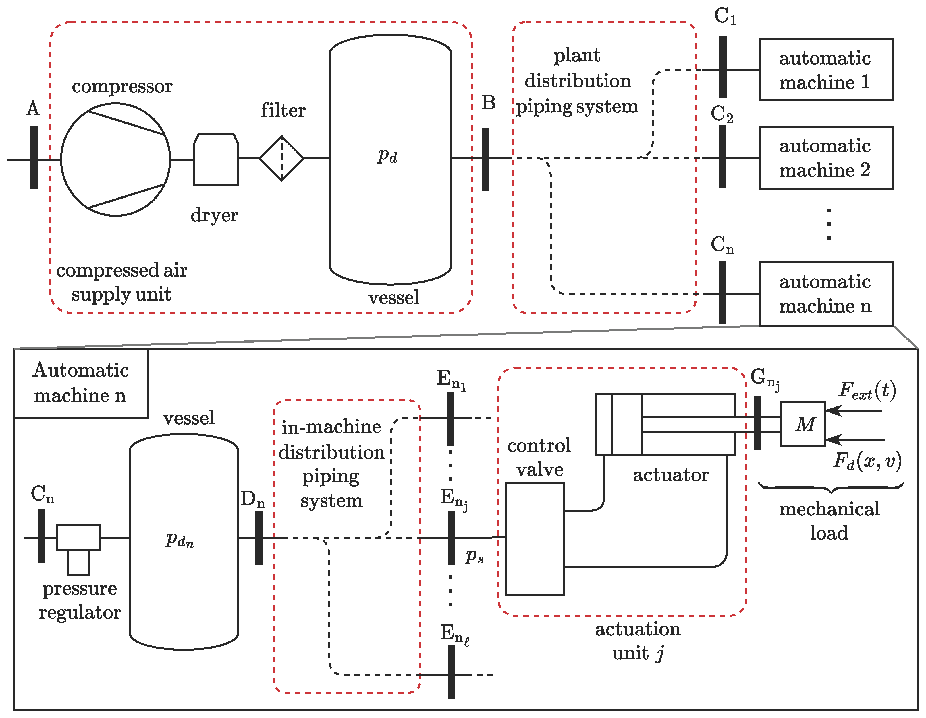
As highlighted in the exploded view in Figure 1, some important sections and components should also be singled out within the generic automatic machine . The latter has, first of all, its own pressure regulator that, starting from the plant-level distribution pressure , sets a machine-specific distribution pressure . The supply pressures powering each actuation unit will then depend not only on , but also on the losses and pressure dynamics that may occur in the in-machine distribution piping system. These losses and variations may be negligible depending on the quality of the design of the in-machine distribution piping system. Finally, the several different actuation units will be suitably controlled and regulated in order to execute the overall machine work cycle. The relevant in-machine sections can be enumerated as follows:
- Section is the outlet port of the vessel, i.e., the inlet port of the distribution piping system.
- Sections to are the inlet ports of the different pneumatic actuation units, each comprising an actuator together with the related valves.
- Section is the mechanical interface of actuator j, representing the link to the mechanical load. The latter is generically represented as a mass M; an applied force , that is a function of time t; and a dissipative force , dependent on position x and speed v.
It should be noted that, among the different highlighted sections, the compressor inlet and the pneumatic actuator mechanical interfaces are the most significant. These indeed represent the input and output power sections of the system that transforms the electrical energy input into useful mechanical work. In pneumatic systems, this transformation necessarily requires the consumption of compressed air. Accurately relating the air mass consumed by the actuator to the electrical energy input to the compressor is the main goal of this work; accordingly, a suitable model of the pneumatic actuator is needed.
2.2. Multi-Physics Dynamic Model of the Actuator
The overall dynamic behaviour of a pneumatic actuator spans three distinct physical domains, namely, the mechanical, gas, and thermal ones, as shown in Figure 2a. The figure depicts all the main components of the pneumatic actuation unit required in a typical application: the pneumatic cylinder; the piston; the associated piping; and the main control and regulation devices, specifically the directional valve and the two throttle valves. The directional valve routes the supply pressure to one cylinder chamber or the other based on a logical command u. Thanks to the internal structure of each throttle valve, the inflow impedance is minimized, while the outflow orifice can be regulated to achieve a suitable back-pressure that leads to the desired piston motion characteristics.
Figure 2.
Actuator domains and control volumes. (a) Actuation unit scheme and physical domains: mechanical (green), gas (dark yellow), and thermal (red). (b) Control volumes, state variables, and mass and thermal flows of the generic side z of the actuation unit.
The mechanical domain allows the description of the motion dynamics of the actuator as a function of the connected masses and of the forces acting on the piston. The pressure inside the actuator chambers and the air mass flow through the actuator control valves are analysed in the gas domain. The heat transfer between the air within the cylinder chambers (and within the associated pipes) and the external environment should be treated in the thermal domain.
2.2.1. Modelling in the Mechanical Domain
The mechanical domain is represented in green in Figure 2a; it consists of the piston, the payload, and the applied forces. The load is represented by the general external force and by the dissipative force . Moreover, inertia actions due to the total mass M and the forces generated by the air pressure in the two chambers are also applied to the piston. Hence, the dynamics of the piston can be described by the following equilibrium equation:
where and are forces due to the air pressure acting, respectively, on faces and of the piston, while is the force due to the ambient pressure on the cross-section of the piston rod.
2.2.2. Modelling in the Gas Domain
For modelling purposes, a linear pneumatic actuation unit can be decomposed into two parts, labelled and , governed by formally identical equations. As represented in Figure 2b, the generic side z is composed of a cylinder chamber, the associated pipe, the throttle valve, and a 3/2 valve representing one half of the overall 5/2 directional valve.
The figure also highlights that there is a fixed control volume for the pipe and a deformable one for the chamber, the associated state variables, and the mass and thermal flows.
The modelling in the gas domain was performed under the assumptions of perfect gas behaviour, neglecting both leakages and the air’s kinetic and potential energies. The Reynolds transport theorem [37,38], applied to mass and enthalpy in the two control volumes depicted in Figure 2b (in which the state variables are assumed to be spatially homogeneous) yields the following equations:
In the equations above, p indicates pressure, V volume, and T temperature, while , , and are the associated time derivatives. The mass of the fluid in the control volume is denoted as m, while q represents the mass flow rate. The symbol R identifies the specific gas constant, is the isochoric specific heat capacity, and is the specific heat ratio; finally, denotes the heat flow rate. The subscripts and stand for “chamber z” and “pipe z”, respectively. Furthermore, the subscripts and indicate quantities related to the flows through the throttle and the directional valves on side z of the actuation unit. In particular, refers to the temperature of the fluid passing through the throttle valve, corresponding either to or to depending on the direction of the flow. Similarly, refers to the temperature of the fluid passing through the directional valve, that corresponds either to or to the supply fluid temperature depending on the direction of the flow. Equations (6)–(9) must be completed with additional relationships that express the valve way flows and as a function of the state variables , , , and . With reference to the ISO 6358-1:2023/Amd.1:2020 standard [39], a valve way behaves similarly to a nozzle, in that the air mass flow rate through the valve ports depends on the valve characteristics, on the duct upstream pressure , and on the downstream pressure . The standard, neglecting any air leakage, defines four valve characteristic coefficients: the sonic conductance C, the critical back-pressure ratio b, the subsonic index m, and the cracking pressure . For industrial pneumatic components, the subsonic index is approximately ; the cracking pressure is usually zero, except for devices that, by design, open only after a certain pressure differential threshold, such as pressure regulators and check valves. The two remaining parameters for the definition of the valve mass flow rate can be obtained experimentally, as discussed in [40], or from the component data sheet.
The mass flow rate in the active valve way, positive when flowing from the port at a higher pressure () to the one at a lower pressure (), is given by
Defining the pressure ratio , the function is written as follows:
The no-flow condition corresponds to , whereas corresponds to a choked sonic flow; in between, for , the flow is subsonic.
Concerning the throttle valve, the mass flow rate is considered positive if entering the actuator chamber. Accordingly, it may be expressed as
This formulation accounts for the asymmetric behaviour of this pneumatic component through the introduction of distinct conductance, critical back-pressure ratio, and cracking pressure parameters: the in-built check valve is characterized by the parameters , , and , while the behaviour of the throttling orifice requires separate and parameters, and a null cracking pressure.
The mass flow rate through the 3/2 directional valve of Figure 2b on the other hand is
where and represent the pressure and temperature of the flow that supplies the directional valve. In general, therefore, , even though the ambient pressure and temperature and can be assumed to be constants in the typical measurement or simulation interval; and can also often be considered constant, provided that the supply system is properly designed.
Most commonly, all the ways of the 5/2 valve display the same behaviour; hence, one conductance and a single critical back-pressure ratio are sufficient to characterize the entire device.
2.2.3. Modelling in the Thermal Domain
In a pneumatic actuation unit, the thermal exchange mainly occurs between the environment and both the cylinder chambers and pipes [33,41,42]. Accordingly, the thermal domain is marked in red in Figure 2b, highlighting the thermal energy transfers and . Heat exchange between air flowing in a pipe or chamber and the environment can be modelled via the following:
- Internal convection, dependent on the local flow and thermodynamic state;
- Wall conduction;
- External natural convection and radiation, both driven by the temperature differential between the outer wall surface and its surroundings.
For a given pipe or chamber, the heat rate can then be expressed under the proposed modelling approach as a function of the internal state, the internal flow, and the ambient temperature, with geometry and material properties treated as fixed parameters. In general terms, the following functional dependencies may be written:
The specific heat transfer regime occurring between the control volumes and the external environment is bounded by two limiting conditions: the adiabatic one, with null heat flux occurring between the two; and the isothermal, characterized by a constant fluid temperature enforced through suitable values assigned to the heat exchange terms. In the subsequent discussion, emphasis is not placed on the detailed thermal modelling of the system, but rather on the analysis of these two envelope cases.
2.2.4. Complete Multi-Domain Model
The complete dynamic model may be obtained by assembling the equations of the different domains, leading to a system of ten first-order differential equations. The state vector is defined as follows:
Then, , , , and can also be straightforwardly expressed as functions of the state variables x and v. Considering together the mechanical equilibrium at the piston and the models in the gas and thermal domains for chambers and pipes and , the complete multi-domain model of the pneumatic actuator is obtained in the form:
or more compactly as
2.3. Experimental Validation of the Multi-Domain Model
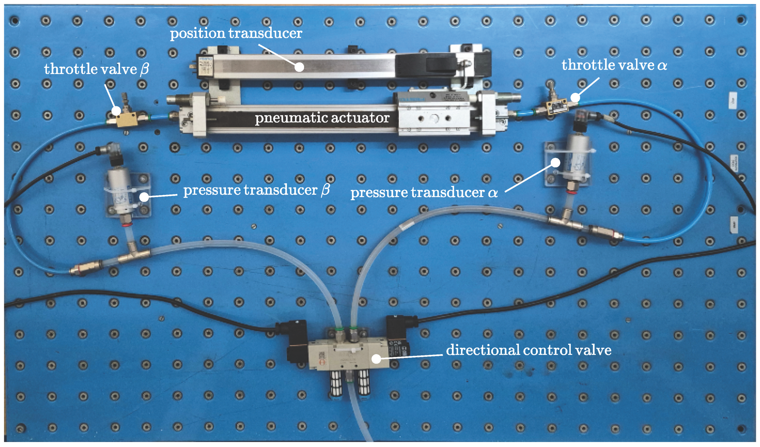
In this paper, the authors evaluate the air mass consumed by the actuator, relying primarily on a simulation approach based on the multi-physics dynamic model described in Section 2.2. The present section deals therefore with its validation, which was achieved through several experimental activities performed on a suitably configured test rig, as shown in Figure 3. The experimental apparatus was equipped with a FESTO (Festo AG & Co. KG, Esslingen am Neckar, Germany) DGPL pneumatic linear drive, a Metal Work (Metal Work S.p.A., Concesio, Italy) series 70 directional valve, a position transducer to measure the position of the actuator piston, and two pressure transducers to measure the pressure in both the actuator chambers. A third pressure gauge was used to monitor the supply pressure. The details concerning the test rig components are summarized in the following list:
- Pneumatic actuator: FESTO DGPL-25-300-PPV-A-B-KF-GK-SH-D2, with a maximum stroke of 300 , and a bore diameter of 25 .
- Directional control valve: Metal Work SOV 35 SOB 00, 5/2 configuration; conductance equal to Nm3Pa−1s−1; critical pressure ratio equal to .
- Position transducer: FESTO MLO-POT-300-TLF (potentiometer with a resolution).
- Pressure transducers: FESTO SDE-10-10V/20mA, with a measuring range of 0 bar to 10 bar.
- Throttle valves: PNEUMAX (Pneumax S.p.A., Lurano, Italy ) 6.01.18N.
Figure 3.
Test rig.
During the course of the experimental tests, care was taken to record the chamber and the directional valve supply pressures , , and , along with the piston stroke x. Then, the experimentally recorded was applied as a time-varying boundary condition to the numerical model, enabling a fair comparison between the measured and simulated time histories of , , and x; both limiting heat exchange conditions, the adiabatic and isothermal ones, were considered in the simulations. The measured and simulated pressures in chambers and are reported in Figure 4a, while Figure 4b compares the numerical and experimental position responses; from these figures it can be ascertained that the different modelling assumptions concerning heat transfer have a minimal impact, as the simulated results issuing from both adequately match the experimental data.
Figure 4.
(a) Pressures in chambers and . (b) Piston position.
Table 1 reports a quantification of the following modelling errors, calculated according to the experimental observations on the one hand, and to the results provided by the isothermal and adiabatic dynamic models on the other: the time-to-end-stop error , the position error , and the pressure errors and . The position and pressure errors are computed in RMS terms, and expressed as a percentage, respectively, of the total stroke and of the full range of pressure variation. Finally, the time-to-end-stop error is computed as , where and indicate, respectively, the simulated and experimental results.
Table 1.
Time -to-end-stop, position, and pressure modelling errors.
This validation step confirms that the multi-physics dynamic model of the valve–actuator system described in Section 2.2 is appropriate for the further discussion; moreover, the choice of the thermal condition in which the system is simulated appears to be of minor importance.
2.4. Procedure for the Evaluation of Electrical Energy Consumption
This work proposes a procedure to evaluate the actuator’s energy consumption considering the air mass expended during its cyclic operation. The procedure considers that such an operation is not uniquely defined, since the actuator can be reconfigured to achieve application-dependent piston motion characteristics, which are as follows:
- The stroke, set as acting on the position of the mechanical end-stops.
- The forward and backward motion times, determined with the regulation of the two throttle valves.
- The dwell and stop times, dictated by the switching instants of the directional valve logical command.
These regulations are leveraged in practice to obtain a suitable degree of production flexibility, with the same machine often being reconfigured to adapt to new manufacturing requirements. All these factors, plus the working forces developed during the work cycle, affect the air mass and energy consumption.
As represented in Figure 5, the procedure can be applied either numerically, using the multi-physics model of the pneumatic machinery, or experimentally, directly measuring the air mass expended by the actuator. The simulation approach is the only option during the initial design stage of the machine; a measurement campaign may serve as a definitive confirmation or as a full alternative whenever the equipment is accessible. In either case, the work cycle and the operating conditions must be defined or configured. In particular, if the numerical route is selected, the parameters of the proposed numerical model should first be determined from a careful analysis of the system and of its operating configuration; steps 1a, 2a and 3a address this issue, and can be described as follows.
Figure 5.
Procedure flow chart.
- Analysis of the components of the pneumatic system.
- Definition of the periodically repeated work cycle and of the regulations needed to achieve it; the cycle in particular can be decomposed into sequences of elementary strokes intertwined with dwell and stop times.
- Calculation, using a multi-physics dynamic model, of the air mass consumed by the actuator during the work cycle.
If a fully experimental approach is selected, steps 1b, 2b, and 3b should be taken instead:
- Setup of the work cycle, through suitable configuration of all the adjustable parameters of the actuation unit.
- Definition of the measurement instrumentation and measurement sections: there are several techniques that allow direct or indirect mass flow rate measurements. As will be shown in the following sections, the transient conditions should be properly captured; therefore, care must be taken to select measurement instruments with an appropriate frequency bandwidth. The mass flow measurement instrumentation should be inserted at sections of Figure 1, which correspond to the supply line leading to the 5/2 direction valve. This choice enables the quantification of the air flow towards the actuator using a single measurement instrument.
- Air mass consumption measurement during the configured work cycle.
The experimental approach is more direct, but it requires access to the plant and the installation of suitable measurement equipment, potentially disrupting normal production activities. The numerical approach, on the other hand, does not require any intervention on the system. The equations proposed in Section 2.2 provide a useful starting point for the implementation of a numerical model; nevertheless, as will be discussed in Section 4.2, more detailed treatments are possible, and may be warranted under certain conditions. It may be noted that the proposed assessment procedure is agnostic with respect to the adopted computational tool, provided that the air mass consumption can be evaluated with sufficient accuracy. Accordingly, commercial software packages that already implement sophisticated models of pneumatic systems may also be used effectively.
After determining the air mass expended per cycle, with either method, the corresponding electrical energy consumed by the compressed air supply unit can be evaluated. The calculation is based on the ISO 1217:2009 standard [35], which defines the specific power requirement of the supply unit, that dimensionally corresponds to a power per unit of volumetric air flow or, equivalently, to an energy per unit of volume. This quantity accounts for the effect of all the devices included in the compressed air supply unit at rated supply conditions. In particular, the specific power is evaluated with respect to the thermodynamic process by which the air is brought from its original state at the compressor inlet to the condition at the compressor outlet. Such a process is defined by its delivery pressure and intake volume flow rate.
The specific power requirement depends on the efficiency of the compressed air supply unit as a whole, being affected not only by the design of the device, but also by its actual operating conditions. If is given for a nominal process characterized by a volume flow rate and delivery pressure that do not match the operating ones, the power input of the compressed air supply unit can be obtained by means of proper measurements made on the compressor; these are described and exemplified in the following section.
2.4.1. Experimental Evaluation of the Specific Power Requirement
The specific power requirement of the compressor is often declared by the manufacturer only for a nominal condition, which might not match the field operating point. The experimental evaluation of at the correct operating condition might therefore be required to properly apply the proposed procedure. This evaluation is based on the measurement of the electric power absorbed by the compressor during a tank filling, and of the relevant delivery pressure. Such measurement can be easily made on any compressor installation, usually using the tank placed downstream of the compressor unit. It should be noted that the measurements should be acquired with the compressor in a steady-state condition, with a constant flow rate at the specific supply pressure.
Figure 6a shows the results of a measurement made on a Shamal K25/200 compressor during the filling of a tank up to a 1.1 MPa delivery pressure; specifically, it depicts the behaviour of the compressor’s electric power consumption and of the relevant delivery pressure as a function of time.
Figure 6.
Results of the experimental activities on the compressor unit. (a) Measured compressor power consumption and delivery pressure. (b) Specific power requirement as a function of the compressor delivery pressure.
According to standard [36], the specific power requirement is expressed as
where is the actual electric power consumption of the compressor, known from the measurements. As regards the volumetric flow rate , it can be calculated from the delivery pressure measurement. Using i as the index of a generic measurement point, the mass within the tank at instant can be calculated as
where is the instantaneous compressed air mass density and V is the tank volume. Assuming that the temperature of the compressed air in the tank is constant and equal to the ambient temperature (), the density can be easily calculated using the absolute tank pressure from the ideal gas law as
By evaluating the mass at instant , the mass flow rate at instant , using the condition i, can be estimated using the forward finite difference:
Finally, the volumetric flow rate at the compressor inlet evaluated at each instant is
where is the air mass density at the compressor inlet conditions. Figure 6b shows the relationship between the estimated specific power requirement and the compressor delivery pressure.
Recalling that the specific power requirement can be equivalently interpreted as a power per unit of intake volumetric flow or as an energy per unit of intake volume, the energy per unit of mass can be simply be obtained as
Therefore, the energy required by the compressed air supply unit to restore the air mass consumed in a cycle is
Equation (31) is applicable if the compressor and the associated tank are properly sized, such that the former operates in steady-state conditions while the latter undergoes negligible pressure variations.
3. Results
In this section, the proposed energy consumption assessment procedure is applied to several case studies that were obtained by configuring different working conditions for the same pneumatic actuation unit. The pneumatic elements considered in the simulations are those already used for the experimental activities. The core of the energy consumption assessment procedure, namely, the evaluation of the air mass processed by each actuator during its actual work cycle, is thus exemplified; extensions to a multi-actuator machine or plant are straightforward. Without precluding the possibility of more detailed thermal modelling, the analysed pneumatic system is provisionally supposed to operate under isothermal heat transfer. As will be shown, this condition can be generally expected to result in a slight overestimation of the energy requirements.
Concerning the applied forces, the simulations of the single pneumatic actuator consider three different cases:
- Case A: Pick-and-place operation occurring in a horizontal plane, mainly subject to inertial forces.
- Case B: Pick-and-place operation occurring in a vertical plane; unlike case A, there is a constant weight force acting along the piston’s direction of motion.
- Case C: Execution of a mechanical operation where a constant resistant force acts in the piston motion direction for a portion of the forward stroke.
These cases are representative of typical industrial uses of pneumatic actuators deployed in automatic machines for pick and place and for the execution of assembly or manufacturing operations. For all the cases, a payload has been considered; for case C, the resistant force has been set to 100 , with its action during the forward motion starting at of the piston stroke.
For each case, different work cycles, constituted by four phases—forward motion, dwell, backward motion, and stop—were considered. The stop time is set for all cases and all work cycles at 0.1 s; the regulation of the backward motion throttle valve is constant within each case study. However, each work cycle is characterized by a distinct setup in terms of the following:
- Forward motion end-stop position, expressed as a percentage using the actually configured stroke s, and , the maximal achievable stroke: .
- Regulation of the forward motion throttle valve that results in different maximum forward velocities and thus allows the achievement of the desired actuation time.
- Dwell time , i.e., the waiting time before the start of the return motion.
As already noted, these three parameters, and the corresponding regulations, define the work cycle of a typical pneumatic linear actuator, and have relevant effects on the air mass and energy consumption. In particular, physical intuition suggests that the following causal mechanisms are at play:
- (i)
- Longer dwell phases provide additional time for the emptying of the actuator chamber.
- (ii)
- Higher velocities are obtained, increasing the conductance of the throttle valve, leading to faster air expulsion from the emptying chamber.
- (iii)
- Larger end-stop positions imply a larger final volume of the emptying actuator chamber, which in turn leads to slower air mass discharge into the environment.
All of the above will be confirmed by the numerical experiments presented in the following subsections, which are obtained from the multi-domain model of Section 2.2.
Effect (i) is self evident; in addition to numerical evidence, effects (ii) and (iii) can be highlighted analytically using a simplified model of the pressure dynamics that occur in the emptying actuator chamber once the piston has reached the end-stop. In particular, considering isothermal heat transfer conditions and an always-sonic discharge flow, Equations (2) and (10) lead to
where is the equivalent discharge conductance due to the throttle and directional valves, and is the volume of the chamber at the end-stop. This linear first-order differential equation is characterized by the following time constant:
which directionally confirms that faster air discharge is correlated directly with (effect (ii)) and inversely with (effect (iii)).
Beyond these insights, the time constant will be used in the following subsections to express in non-dimensional form the duration of the dwell phase as the time ratio . Given this definition, the parameter synthetically accounts for the combined effects (i), (ii), and (iii).
For each case, three sets of nine work cycles were considered; for each set, one of the three piston motion characteristics listed above was kept constant, while different combinations of the remaining two were considered. For example, in the first set of simulations, the regulation of the forward motion throttling valve is fixed, while several combinations of end-stop position and dwell time are analysed. To show the influence of the three varying parameters on the overall energy consumption, each simulation focuses on the evaluation of the air mass discharged during the work cycle. The single period reported for each work cycle is the one at which truly periodic operating conditions are established.
For each test case, the results are summarized in pairs of tables (e.g., Table 2 and Table 3), where the energy consumption corresponding to the discharged air mass is reported, along with the ratio . Every simulation is indicated by a capital letter with three subscript indices. The letter refers to the application case, while the indices identify the specific work-cycle configuration: the first (i) refers to the end-stop position, the second (j) refers to the piston velocity, and the third (k) refers to the dwell time. For example, with reference to Table 2, A131 corresponds to the simulation of case A with a work-cycle configuration characterized by end-stop position (i = 1), of 1 m/s (j = 3), and dwell time of s (k = 1).
Table 2.
Value of in [J] for cases ; piston velocity equal to 1 m/s.
Table 3.
Value of for cases ; piston velocity equal to 1 m/s.
3.1. Case A
In case A, the piston moves horizontally, subject only to inertial forces. The simulation results are reported in Table 2, Table 3, Table 4, Table 5, Table 6 and Table 7 and in Figure 7, Figure 8 and Figure 9.
Table 4.
Value of in [J] for cases A3jk; end-stop position equal to 20%.
Table 5.
Value of for cases A3jk; end-stop position equal to 20%.
Table 6.
Value of in [J] for cases Aij1; dwell time equal to 0.1 s.
Table 7.
Value of for cases Aij1; dwell time equal to 0.1 s.
Figure 7.
Case A: position and pressure behaviour for piston velocity = 1 m/s. (a) Position. (b) Pressure.
Figure 8.
Case A: position and pressure behaviour for end-stop position = . (a) Position. (b) Pressure.
Figure 9.
Case A: position and pressure behaviour for waiting time = 0.10 s. (a) Position. (b) Pressure.
Table 2 and Table 3 report the results of the simulations performed at a fixed throttle valve regulation that leads to a maximum forward piston velocity of 1 m s−1. Effect (i) is not visible along the first row of Table 2 due to the fact that, as shown in Figure 7b, in simulations A131, A132, and A133 the pressure in chamber reaches ambient pressure at the end of the dwell phase. This means that the chamber has been completely discharged, and that consequently the air mass consumption is the same. The dwell time effect is however apparent along row two of the table: all the simulations correspond to a end-stop position, but A231 has an energy consumption lower than A232 and A233. In fact, the pressure graph of A231 shows that in this condition the dwell time is not enough to lead to the ambient pressure in chamber ; hence, in this case the air mass consumption is lower than in A232 and A233, where reaches the ambient value. Also, for A331, A332, and A333 similar considerations apply. Effect (iii) is clear along all the columns of Table 2.
Figure 7a represents the time history of the piston position for all simulations summarized in Table 2 and Table 3. The forward motion speed is the same, while the piston end positions change according to the different end-stop configurations. The backward motion starts at different instants due to the combination of different end-stop positions and dwell times.
A comparison between Figure 7a,b shows that during the initial portion of the forward stroke, the motion and pressures dynamics all have the same behaviour, since the throttle valve setup is identical for all the simulations. The plots start to deviate from each other only after the piston reaches the end-stop and the dwell phase starts; at that instant, the pressure starts decreasing due to the ongoing discharge of the residual air mass. Once the directional valve switches to start the backward motion, the pressure quickly rebounds to the supply pressure value. During the backward stroke the pressure then decreases slightly due to the chamber expansion; it stabilizes once again after the end-stop is reached, and remains constant at the supply pressure value until the end of the cycle.
Table 4 and Table 5 report the results obtained when keeping the end-stop position constant and equal to . As seen in the piston motions in Figure 8a, forward speed and dwell times vary.
The simulations displaying the same velocity (e.g., A311, A312, A313) show an energy consumption increase for longer dwell phases (effect (i)). This is confirmed by the pressure dynamics depicted in Figure 8b, which show that the residual pressure decreases from A311 to A313. The same happens along the other rows of Table 4, where, by increasing the dwell time, the pressures ultimately reach the ambient value. With constant dwell time, on the other hand, energy consumption is positively correlated with , i.e., with the higher conductance settings of the throttle valve (effect (ii)). As shown in Figure 8b, this leads to faster air mass discharge and progressively decreasing residual pressures in, e.g., cases A311, A321, and A331.
A comparison between Figure 8a,b shows that during the backward stroke, the motion and pressure dynamics are similar to those of the previous set of simulations. By contrast, during the forward motion, the graphs display different behaviours due to the varying throttle valve regulation.
Table 6 and Table 7 report the results obtained when keeping the dwell time constant, equal to . Figure 9a shows that the differences concern the forward motion velocity and the piston final position. For these configurations, similarly to the previous set of simulations, energy consumption is correlated directly with the velocity, (effect (ii)) and inversely with end-stop positions (effect (iii)). Again, this result is confirmed by the graphs of the pressure in Figure 9b.
3.2. Case B
In this application case, the actuator piston moves vertically, and is subjected to inertial and gravitational forces due to the piston and payload masses; in particular, gravity opposes the forward motion and aids the backward one. The simulation results are reported in Table 8, Table 9, Table 10, Table 11, Table 12 and Table 13, and in Figure 10, Figure 11 and Figure 12. The results are very similar to case A, for each set of simulations; this means that the considered weight force does affect significantly the total air mass consumption. The results of the set of simulations collected in Table 8 and Table 9 are in particular very close to those of Table 2 and Table 3 respectively, exception made for simulation B331 where the dynamic behaviour of the system leads, at the end of the cycle, to a slightly higher energy consumption compared to case A331. The values of the ratios in Table 9 match those of Table 3, because depends only on the chamber volume and the discharge motion. Figure 10a shows that the forward velocities are equal to each other, and to the velocities of the first simulation set of case A. A difference with respect to case A concerns the reduced maximum velocity of the return motion: in case B, in fact, a controlled payload descent is obtained through a suitable regulation of the backward stroke throttle valve.
Table 8.
Value of in [J] for cases Bi3k; piston velocity equal to 1 m/s.
Table 9.
Value of for cases Bi3k; piston velocity equal to 1 m/s.
Table 10.
Value of in [J] for cases B3jk; end-stop position equal to 20%.
Table 11.
Value of for cases B3jk; end-stop position equal to 20%.
Table 12.
Value of in [J] for cases Bij1; dwell time equal to 0.1 s.
Table 13.
Value of for cases Bij1; dwell time equal to 0.1 s.
Figure 10.
Case B: position and pressure behaviour for piston velocity = 1 m/s. (a) Position. (b) Pressure.
Figure 11.
Case B: position and pressure behaviour for end-stop position = . (a) Position. (b) Pressure.
Figure 12.
Case B: position and pressure behaviour for waiting time = 0.10 s. (a) Position. (b) Pressure.
The energy consumption varies in response to the different work-cycle parameters, similarly to case A. For example, in simulations B131–B133 the energy consumption does not change, since the residual reaches the ambient pressure. By contrast, in simulations B231 and B331 the energy consumption does not reach the maximum possible value because the dwell phase stops before the complete discharge of the chamber. Finally, effect (iii) clearly appears along the columns of Table 8. In Figure 10a it can be seen that the backward motions start at distinct instants due to the different combinations of end-stop positions and dwell times. Also, observing Figure 10b it appears that during the forward motion, the pressure graphs initially display the same behaviour, as the throttle valve regulation is shared by all the simulated configurations. The differences occur when each piston reaches the end-stop and the dwell phase starts; the pressure first decreases, then rebounds to the supply pressure value once the backward motion starts; in case B, no further significative variation occurs during the return motion.
Due to the low influence of the vertical configuration of the actuator, the data reported in Table 4 and Table 10 are also similar; those in Table 5 and Table 11 are identical due to the definition of . Effects (i) and (ii) can be seen, respectively, along the rows and columns of Table 10. This can be confirmed by analysing the residual pressure values at the end of the dwell phases in Figure 11b.
Examination of Figure 11a,b shows that during the forward motion, the different throttle valve regulations lead to distinct motion and pressure dynamics; after the pressure increase due to the switching of the directional valve, the return motion is then uneventful.
Table 12 and Table 13, reporting the results of the simulations for a constant dwell time equal to , are, respectively, very similar and identical to Table 6 and Table 7, supporting already familiar considerations concerning effects (ii) (along the columns) and (iii) (along the rows). Together, Figure 12a,b show that the different pressure dynamics during the forward motion correspond to different velocities and throttle valve regulations; on the other hand, the pressure during the return motion is practically constant and equal to the supply pressure.
3.3. Case C
In case C the piston moves horizontally, and is subject to a constant force that opposes a portion of the forward motion. While cases A and B are similar to each other in terms of energy consumption, Table 14, Table 15, Table 16, Table 17, Table 18 and Table 19 and Figure 13, Figure 14 and Figure 15 show that case C is noticeably different.
Table 14.
Value of in [J] for cases Ci3k; piston velocity equal to 0.2 m/s.
Table 15.
Value of for cases Ci3k; piston velocity equal to 0.2 m/s.
Table 16.
Value of in [J] for cases C3jk; end-stop position equal to 20%.
Table 17.
Value of for cases C3jk; end-stop position equal to 20%.
Table 18.
Value of in [J] for cases Cij1; dwell time equal to 0.1 s.
Table 19.
Value of for cases Cij1; dwell time equal to 0.1 s.
Figure 13.
Case C: position and pressure behaviour for piston velocity = 0.2 m/s. (a) Position. (b) Pressure.
Figure 14.
Case C: position and pressure behaviour for end-stop position = . (a) Position. (b) Pressure.
Figure 15.
Case C: position and pressure behaviour for waiting time = 0.10 s. (a) Position. (b) Pressure.
These differences are mainly due to the lower velocities (and higher throttling) that characterize case C, as reported in Table 16 and Table 18. Table 14 and Table 15 report the results at equal to /. Case C deviates from cases A and B in terms of values due to the lower discharge conductance, which implies a higher time constant .
The dependence of the energy consumption on the work-cycle parameters follows the same trends stated for the previous cases: as the end-stop position increases at constant dwell time, the energy consumption decreases, whereas it increases for longer dwell phases at a constant end-stop position.
As before, the value of the residual pressure at the end of the dwell phase reveals whether chamber is completed discharged. For example, it is clear in Figure 13b that the only configuration in which the chamber completely empties is C133, for which the residual pressure reaches the ambient value. The energy consumption is therefore equal to that of configuration A133. As observed in Figure 13a,b, the main differences with respect to cases A and B concern the temporary change in velocity and the pressure drop during the forward motion. Both are due to the sudden action of the resistant force, whose action starts at a fixed fraction of the configured piston stroke. The pressure transient is evident in Figure 13b, where decreases approximately from to . Then, similarly to cases A and B, the pressure switches to the supply pressure value as the backward motion starts; in case C, no pressure drop is subsequently observed.
Table 16 and Table 17 report the results for a constant end-stop position equal to ; they support the same considerations already discussed in the corresponding sets of simulations of cases A and B. The main difference with respect to the results reported in Table 14 and Table 15 is that the value of the residual pressure never reaches the ambient pressure, meaning that the air mass in chamber does not completely discharge.
Similarly to the immediately preceding set of simulations, Figure 14a,b display transient ranges associated with the onset of the resistant force, with the timing being affected by the different velocities. During the forward motion, the pressure dynamics are unique to each simulation due to the different throttling regulations; during the backward stroke, on the other hand, they follow a shared pattern.
Table 18 and Table 19 report the results of the last set of simulations, performed at a constant dwell time equal to . In this set, no configuration achieves the complete discharge of chamber . This is highlighted by the plots of in Figure 15b, which all remain always above the ambient pressure.
The remarks already made for the analogous sets of simulations of cases A and B (Table 6, Table 7, Table 12 and Table 13) are also applicable here: effect (ii) is apparent along the rows of Table 18, while (iii) is evident along the columns.
Similarly to the other simulation sets in case C, the resistive force induces motion and pressure transients (as seen in Figure 15a,b), starting at the same fraction of the forward stroke. The pressure dynamics are not uniform across the different simulations during the forward motion due to the effect of the different throttling regulation, corresponding to different velocities; on the contrary, the behaviour during the backward stroke is similar.
4. Discussion
Concerning effects (i), (ii), and (iii) described in Section 3, they are ultimately linked to the transient dynamics of the system: if enough time—for given conductance and residual volume values—is provided for the achievement of steady-state conditions, the air and energy consumption is maximized. On the contrary, if the emptying chamber is not allowed to reach an equilibrium with the environment, the residual air mass does not need to be restored by the compressor unit and can be used for the return stroke.
The graphical representation in Figure 16 summarizes all the simulations performed to analyse case A. The figure depicts in particular the behaviour of the energy consumption as a function of the non-dimensional ratio . Also the energy consumption is expressed in a non-dimensional form, using a suitably defined energy ratio , in which the numerator is the energy consumption and the denominator corresponds to the energy consumed when the chambers are in turn completely discharged during a work cycle. This latter value corresponds to the air mass consumption calculated according to more traditional approaches that consider just the geometry of the actuator chambers, neglecting the work-cycle parameters.
Figure 16.
Synthetic representation of the simulation results concerning case A.
The data represented in Figure 16 are grouped according to the end-stop position. Analysis of the relevant graphs leads to interesting considerations: first of all, the plot highlights that the energy consumption depends on the dynamic behaviour of the system; secondly, there is a value of beyond which the energy ratio becomes unitary for any end-stop position value. This means that if is greater than a particular value (approximately equal to 2, for this set of configurations), the air mass consumption can be calculated with the commonly used steady-state method that considers just the geometry of the actuator. On the contrary, if , the actual air mass consumption is lower than that calculated with the usual method, which would lead to an overestimation of the energy consumption. The maximum overestimation would be approximately equal to of the value obtained with the proposed method.
Figure 17 depicts a synthetic representation of the data obtained from all simulations concerning case B. The graph of Figure 17 is very similar to the graph of Figure 16. Hence, in this case it is also possible to highlight that after a specific value of the non-dimensional time ratio , the energy ratio is 1 for any end-stop position configuration, confirming that if , the energy consumption can be evaluated according to the traditional methodology; on the contrary, if , the usual approach leads to an overestimation of the energy consumption that, also in this case, has a maximum value of approximately of the value obtained with the proposed method.
Figure 17.
Synthetic representation of the simulation results concerning case B.
Finally, Figure 18 summarizes the data gathered when analysing case C, grouped according to the end-stop positions. As for case A and case B, the energy consumption is represented in non-dimensional form as a function of the non-dimensional variable . Mainly due to the difference in the values of , this plot differs slightly from those of case A and case B. However, a similar consideration can be drawn: as the value of increases, the energy ratio ultimately reaches the unit value. In particular, it also appears from Figure 18 that the value of beyond which the energy ratio is equal to 1 is again approximately equal to 2. In this case, the maximum overestimation is slightly lower than .
Figure 18.
Synthetic representation of the simulation results concerning case C.
The specific threshold remains an empirical observation; however, the overall trend of increasing with is a robust and repeatable finding grounded in both theoretical and numerical evidence.
4.1. Model Sensitivity to Heat Transfer Conditions
As already highlighted in Section 2.2.3, two limiting heat transfer conditions, namely, the isothermal and the adiabatic ones, may be considered to bound the numerical evaluation of the overall electrical energy consumed during a work cycle. While any other heat transfer condition can be modelled within the overall methodology proposed by the authors, the experimental data presented in Section 2.3 suggest that the simulation results are quite insensitive to the assumed heat transfer regime. To supplement this evidence, a few selected cases have been re-analysed considering both isothermal and adiabatic conditions. The results of these simulations are visualized in Figure 19.
Figure 19.
Comparison between the compressor energy consumption assuming either isothermal or adiabatic thermal exchange. The comparison is made for three of the configurations described in Section 3.
The bar graph shows that for any configuration (A331, B111, C231), the energy consumption of the compressor unit is, as expected, highest in the case of isothermal condition and lowest in the adiabatic simulations; however, the gap between the two is narrow. In general, it can be concluded that, from an engineering point of view, it is appropriate to consider the isothermal heat exchange; this, on the one hand, constitutes a precautionary assumption, but at the same time does not deviate significantly from any realistically occurring heat transfer condition.
4.2. Augmented Modelling Approach for Non-Ideal Supply Systems
As discussed in Section 2.3, the results of the experimental activities allowed the validation of the model of the actuation unit from the directional control valve to the load, i.e., of a model that accounts for the directional control valve, the throttle valves, and the actuator (DTVA model in short). Even though the lumped-parameter model was shown to be quite accurate, its behaviour is affected by the boundary condition that defines the pressure at the inlet of the directional valve. In a carefully sized system, such a pressure may be well approximated with a constant value; the simulations presented in Section 3 were performed under this modelling assumption. In cases where this hypothesis is not verified, the boundaries of the computational model must be extended to include the additional pneumatic components needed to properly model the pressure dynamics at the directional valve inlet.
Hence, the DTVA model has been extended, as represented in Figure 20, to include three additional components: a pressure regulator, a vessel, and the in-machine distribution pipes. This additional equipment can be modelled and simulated relying on models and algorithms available in the current literature: see [43,44,45,46] for the modelling of the pressure regulator, and [47,48,49,50] for the pneumatic transmission lines. In the extended model, each pipe is not modelled using a single control volume, but rather discretized using the MacCormack finite difference method.
Figure 20.
Components considered in the extended model.
The overall extended model was adapted to the test rig configuration described in Section 2.3, which, in addition to the already described components, features the following:
- A L vessel;
- An 8 -long pipe with a 25 diameter that connects the pressure regulator and the vessel;
- A -long pipe with an 8 diameter that connects the vessel to the directional valve;
- A -long pipe with a 6 diameter that connects the directional valve to chamber of the actuator;
- A -long pipe with a 6 diameter that connects the directional valve to chamber of the actuator.
The grid spacing used to discretize the piping is equal to 10 , while the time step of was selected in order to satisfy the Courant–Friedrichs–Lewy condition and thus ensure stability. Figure 21, Figure 22, Figure 23 and Figure 24 show the results obtained simulating the behaviour of the system when the extended model is used.
Figure 21.
Pressure in chamber : comparison between experimental and extended simulation results.
Figure 22.
Position and pressure behaviour for end-stop position = : comparison between DTVA and extended model simulations. (a) Position. (b) Pressure.
Figure 23.
Position and pressure behaviour for end-stop position = : comparison between DTVA and extended model simulations. (a) Position. (b) Pressure.
Figure 24.
Position and pressure behaviour for end-stop position = : comparison between DTVA and extended model simulations. (a) Position. (b) Pressure.
In particular, Figure 21 depicts the comparison between the experimental behaviour of the pressure in actuator chamber , already discussed in Section 2.3, and the corresponding extended model simulation result. The figure shows that the model approximates the experimental results well, being able to reproduce pressure dynamics that exhibit an initial increase until around MPa, a following decrease at about MPa, and a final slow increase until the nominal supply pressure value. The air mass and energy consumption is affected by the dynamics of the entire machine, inclusive of the pressure regulator and air distribution system. Other simulations were therefore performed using the model extension in conditions where these additional dynamics cannot be neglected.
In particular, cases A131, A231, and A331, whose characteristics are highlighted in Table 2 and Table 3, are again simulated; the results are then compared to those obtained using the DTVA model. Figure 22, Figure 23 and Figure 24 report the comparison between the results of the extended and DTVA model simulations for two cycles of motion. In particular, the behaviour of the actuator position and of pressure are depicted; for all the three simulations, it is clearly shown that the behaviour of the actuator changes both in terms of position and in terms of pressure. As regards Figure 22a–Figure 24a, the graphs of the position show that DTVA model exhibits a behaviour very similar to extended one, but with a significant delay. Such a delay can be imputed to the pressures in the actuator chambers; in fact, with reference to Figure 22b–Figure 24b, the pressures concerning the extended model are rather different from the corresponding pressures obtained from the DTVA model. Moreover, the pressure differences between the DTVA and extended models lead to a different, and lower, evaluation of the air mass consumption. Therefore, it can be concluded that even when the supply pressure displays significant dynamics, the extended model still allows an accurate evaluation of the energy consumption. Considering the work cycles arising from the considered set of actuation unit regulations together with the pressure dynamics as evaluated with the extended model, it can be seen that the energy consumption overestimation obtained from the traditional steady-state evaluation is as follows:
- 36.96% for case ;
- 37.77% for case ;
- 41.38% for case .
The results presented in Figure 16, Figure 17 and Figure 18 are representative of a situation where the only relevant dynamics are introduced by the actuation unit; the time ratio was therefore defined using a time constant that reflects the actuator chamber characteristics. For the more complex cases analysed in this section, a different reference time constant should be defined, considering all the components that determine the overall dynamic behaviours.
5. Conclusions
This paper presents a new procedure for the assessment of the electrical energy needed to perform specific functions in industrial machines by means of pneumatic actuators. Differently from other approaches available in the literature, the proposed procedure is based on the dynamic behaviour of the system, both from the mechanical and the pneumatic points of view. The procedure can be broadly applied to any pneumatically actuated automatic machine, regardless of the related work-cycle complexity; moreover, the procedure allows the user to choose the approach considered most suitable for the evaluation of the air mass consumption, whether numerical or experimental.
The results obtained from the analysis of different application cases show an overestimation of the air mass and of the electrical energy consumption if the traditional method that considers the steady-state behaviour of the system is adopted. Hence, the proposed procedure allows a more accurate assessment of the consumption related to each specific application for which the actuators are used, considering the transient dynamics of the system and the cyclic behaviour typical of the automatic machines. Furthermore, the procedure enables a precise evaluation of the electrical energy needed to restore the consumed air mass in the operating conditions by tailoring the ISO 1217 standard for the evaluation of the compressor performance to its actual working conditions. Future work will address the application of the procedure to more complex systems where many actuators are simultaneously used, as occurs in an automatic machine for assembly or pick-and-place operations. As a further activity, the authors are planning to use the proposed procedure to make an energy comparison between machines performing similar operations with different driving technologies.
Author Contributions
Conceptualization, P.R. and R.S.; methodology, P.R., R.S. and F.C.; software, R.S.; validation, P.R., R.S. and F.C.; investigation, P.R. and R.S.; writing—original draft preparation, P.R., R.S. and F.C.; writing—review and editing, F.C.; supervision, P.R. All authors have read and agreed to the published version of the manuscript.
Funding
The research was funded by the University of Bergamo; fund code: 60RIGH24.
Institutional Review Board Statement
Not applicable.
Informed Consent Statement
Not applicable.
Data Availability Statement
Data is contained within the article.
Conflicts of Interest
The authors declare no conflicts of interest.
Nomenclature
| State-dependent system matrix of the assembled multi-domain model | |
| Gas-domain submatrix for generic side z ( or ) | |
| Mechanical coupling submatrix for generic side z ( or ) | |
| Kinematic submatrix | |
| Effective cross-sectional area of generic chamber z ( or ) | |
| b | ISO 6358 critical back-pressure ratio |
| Critical back-pressure ratio of check valve z | |
| Critical back-pressure ratio of directional valve z | |
| Critical back-pressure ratio of throttle orifice z | |
| Additive state-dependent term in the assembled multi-domain model | |
| Mechanical additive term in the multi-domain model | |
| Gas/thermal additive term for generic side z ( or ) in the multi-domain model | |
| C | ISO 6358 sonic conductance |
| Sonic conductance of check valve z | |
| Sonic conductance of directional valve z | |
| Equivalent sonic conductance between chamber z and the environment | |
| Sonic conductance of throttle orifice z | |
| Specific isochoric heat capacity | |
| Electrical energy consumption per work cycle | |
| Electrical energy per unit of compressed air mass | |
| Energy ratio | |
| Dissipative force acting on the piston | |
| External mechanical load acting on the piston | |
| Heat capacity ratio | |
| Mass flow function for directional valve z | |
| ISO 6358 mass flow function | |
| Specific enthalpy of the flow through the directional valve on side z of the actuation unit | |
| Specific enthalpy of the flow through the throttle valve on side z of the actuation unit | |
| Air mass consumed per work cycle | |
| Air mass in generic chamber z | |
| Air mass inside the compressor tank at time | |
| M | Moving mass in the mechanical domain |
| Air mass in the pipe on generic side z | |
| m | ISO 6358 subsonic index |
| Ambient pressure | |
| Pressure in generic actuator chamber z | |
| Plant distribution pressure | |
| Distribution pressure of automatic machine | |
| Downstream pressure in the ISO 6358 valve way model | |
| RMS pressure modelling error in generic actuator chamber z | |
| Compressor tank pressure at time | |
| Pressure in the pipe on generic actuation unit side z | |
| Measured electric power absorbed by compressor unit | |
| Directional valve inlet/supply pressure | |
| Specific power requirement | |
| Upstream pressure in the ISO 6358 valve way model | |
| ISO 6358 non-dimensional flow function | |
| Mass flow rate through the directional valve on generic side z | |
| Estimated tank mass flow rate at sample i from pressure ramp data | |
| Mass flow rate through the throttle valve on generic side z | |
| Volumetric flow rate at compressor inlet conditions | |
| Volumetric flow rate at compressor inlet conditions, evaluated at sample i | |
| Heat transfer rate between the air in generic chamber z and the environment | |
| Heat transfer rate between the air in pipe on generic side z and environment | |
| R | Specific gas constant for air |
| r | ISO 6358 pressure ratio |
| ISO 6358 reference air density | |
| Air density at compressor inlet conditions | |
| Air density in the compressor tank at sample time | |
| End-stop position | |
| s | Configured actuator stroke |
| Maximum actuator stroke | |
| t | Time |
| Time-to-end-stop error | |
| Experimentally measured time to end-stop | |
| Simulated time to end-stop | |
| Dwell time | |
| Sampling time instant associated with measurements | |
| Time ratio | |
| Reference time constant | |
| ISO 6358 reference temperature | |
| Ambient temperature | |
| Temperature in generic chamber z | |
| Temperature of directional valve flow on generic side z | |
| Temperature in pipe on generic side z | |
| Supply air temperature for the directional valve model | |
| Temperature of throttle valve flow on generic side z | |
| ISO 6358 upstream temperature | |
| u | Directional valve command signal |
| v | Piston velocity |
| Maximum piston velocity occurring along the stroke | |
| V | Volume of the compressor vessel |
| Control volume of generic chamber z | |
| Minimum volume of chamber z obtained when the piston is at the end-stop | |
| Control volume of pipe on generic side z | |
| x | Piston position |
| RMS position modelling error | |
| State vector |
References
- Righettini, P.; Strada, R.; Tiboni, M.; Cortinovis, F.; Santinelli, J. A systematic management and control methodology for high energy saving in applications equipped with hydraulic servo-axes. Control Eng. Pract. 2024, 145, 105847. [Google Scholar] [CrossRef] [Scilit]
- Righettini, P.; Strada, R.; Cortinovis, F.; Santinelli, J. New Management Strategy for a Significant Reduction of the Impact on CO2 Footprint of Hydraulic Actuators. In Proceedings of the I4SDG Workshop 2025—IFToMM for Sustainable Development Goals; Carbone, G., Quaglia, G., Eds.; Springer: Cham, Switzerland, 2025; pp. 505–512. [Google Scholar] [CrossRef] [Scilit]
- Righettini, P.; Strada, R.; Cortinovis, F. Application of a New Management and Control Methodology for High Energy Saving in Hydraulic Bending Presses. In Proceedings of the 2024 International Congress on Human-Computer Interaction, Optimization and Robotic Applications (HORA), Istanbul, Turkey, 23–25 May 2024; pp. 1–5. [Google Scholar] [CrossRef] [Scilit]
- Righettini, P.; Strada, R.; Cortinovis, F. Load Simulator Design for the Experimental Validation of a High Energy Saving Methodology in the Automation System of Hydraulic Presses. In Proceedings of the 2024 International Congress on Human-Computer Interaction, Optimization and Robotic Applications (HORA), Istanbul, Turkey, 23–25 May 2024; pp. 1–9. [Google Scholar] [CrossRef] [Scilit]
- Wu, Y.C.; Chen, F.W.; Liao, T.T.; Chen, C.T. Force reflection in a pneumatic artificial muscle actuated haptic system. Mechatronics 2019, 61, 37–48. [Google Scholar] [CrossRef] [Scilit]
- Peng, Y.; Sakai, Y.; Funabora, Y.; Yokoe, K.; Aoyama, T.; Doki, S. Funabot-Sleeve: A Wearable Device Employing McKibben Artificial Muscles for Haptic Sensation in the Forearm. IEEE Robot. Autom. Lett. 2025, 10, 1944–1951. [Google Scholar] [CrossRef] [Scilit]
- Franco, W.; Maffiodo, D.; De Benedictis, C.; Ferraresi, C. Use of McKibben Muscle in a Haptic Interface. Robotics 2019, 8, 13. [Google Scholar] [CrossRef] [Scilit]
- Qi, J.; Gao, F.; Sun, G.; Yeo, J.C.; Lim, C.T. HaptGlove—Untethered Pneumatic Glove for Multimode Haptic Feedback in Reality–Virtuality Continuum. Adv. Sci. 2023, 10, 2301044. [Google Scholar] [CrossRef] [Scilit]
- Lolli, V.; Rovai, A.; Trotta, N.; Bourguignon, M.; Goldman, S.; Sadeghi, N.; Jousmäki, V.; De Tiège, X. MRI-compatible pneumatic stimulator for sensorimotor mapping. J. Neurosci. Methods 2019, 313, 29–36. [Google Scholar] [CrossRef] [Scilit]
- Tiboni, M.; Loda, D. Monolithic PneuNets Soft Actuators for Robotic Rehabilitation: Methodologies for Design, Production and Characterization. Actuators 2023, 12, 299. [Google Scholar] [CrossRef] [Scilit]
- Fan, J.Z.; Zhang, W.; Kong, P.C.; Cai, H.G.; Liu, G.F. Design and Dynamic Model of a Frog-inspired Swimming Robot Powered by Pneumatic Muscles. Chin. J. Mech. Eng. 2017, 30, 1123–1132. [Google Scholar] [CrossRef] [Scilit]
- Harris, P.; O’Donnell, G.E.; Whelan, T. Energy Efficiency in Pneumatic Production Systems: State of the Art and Future Directions. In Proceedings of the Leveraging Technology for a Sustainable World; Dornfeld, D.A., Linke, B.S., Eds.; Springer: Berlin/Heidelberg, Germany, 2012; pp. 363–368. [Google Scholar] [CrossRef] [Scilit]
- Du, H.; Xiong, W.; Xu, C.; Jiangr, Z. Research on the controllability and energy saving of the pneumatic direct drive system. Int. J. Heat. Technol. 2017, 35, 997–1004. [Google Scholar] [CrossRef] [Scilit]
- Krytikov, G.; Strizhak, M.; Strizhak, V. The synthesis of structure and parameters of energy efficient pneumatic actuator. East.-Eur. J. Enterp. Technol. 2017, 1, 38–44. [Google Scholar] [CrossRef] [Scilit]
- Du, H.; Xiong, W.; Liu, W. A Nonlinear Dynamic Optimization Algorithm of a Novel Energy Efficient Pneumatic Drive System. Int. J. Control. Autom. Syst. 2022, 20, 1593–1604. [Google Scholar] [CrossRef] [Scilit]
- Jiang, Z.; Xiong, W.; Du, H.; Wang, Z.; Wang, L. Energy-saving methods in pneumatic actuator stroke using compressed air. J. Eng. 2021, 2021, 241–251. [Google Scholar] [CrossRef] [Scilit]
- Boyko, V.; Weber, J. Energy Efficiency of Pneumatic Actuating Systems with Pressure-Based Air Supply Cut-Off. Actuators 2024, 13, 44. [Google Scholar] [CrossRef] [Scilit]
- Du, H.; Liu, W.; Bian, X.; Xiong, W. Energy-Saving for Industrial Pneumatic Actuation Systems by Exhausted Air Reuse Based on a Constant Pressure Elastic Accumulator. Sustainability 2022, 14, 3535. [Google Scholar] [CrossRef] [Scilit]
- Lu, L.; Kou, J.; Gu, X.; Xu, S.; Wang, Y.; Wu, K.; Shi, Y. Literature Review: Energy Saving of Pneumatic System. In Proceedings of the 2023 9th International Conference on Fluid Power and Mechatronics (FPM), Lanzhou, China, 18–21 August 2023; pp. 1–8. [Google Scholar] [CrossRef] [Scilit]
- Dudić, S.; Reljić, V.; Šešlija, D.; Dakić, N.; Blagojević, V. Improving Energy Efficiency of Flexible Pneumatic Systems. Energies 2021, 14, 1819. [Google Scholar] [CrossRef] [Scilit]
- Jimenez, C.R.; Reinertz, O.; Schmitz, K. A Comprehensive Study of Energy-Saving Strategies Through Combined Throttling. Int. J. Fluid Power 2024, 25, 1–26. [Google Scholar] [CrossRef] [Scilit]
- Vigolo, V.; Boyko, V.; Weber, J.; Valdiero, A.C.; De Negri, V.J. Online Monitoring of Pneumatic Actuation System for Energy Efficiency and Dynamic Performance. In Proceedings of the ASME/BATH 2023 Symposium on Fluid Power and Motion Control, Sarasota, FL, USA, 16–18 October 2023; p. V001T01A054. [Google Scholar] [CrossRef] [Scilit]
- Vigolo, V.; Boyko, V.; Weber, J.; De Negri, V.J. A Model-Based Approach for Online Optimization of Pneumatic Drives. IEEE/ASME Trans. Mechatron. 2025, 30, 4503–4513. [Google Scholar] [CrossRef] [Scilit]
- Boyko, V.; Nazarov, F.; Gauchel, W.; Neumann, R.; Doll, M.; Weber, J. Comprehensive Application-Based Analysis of Energy-Saving Measures in Pneumatics. Int. J. Fluid Power 2024, 25, 27–58. [Google Scholar] [CrossRef] [Scilit]
- Lee, L.W.; Yang, J.Y.; Li, I.H. Enhancing trajectory tracking and energy efficiency in Pneumatic Servo Translational Parallel Manipulator with Frac-SMC-RFESO Control. Control Eng. Pract. 2025, 162, 106372. [Google Scholar] [CrossRef] [Scilit]
- Irawan, A.; Suid, M.H.; Ismail, R.R.; Jusof, M.F.M.; Azahar, M.I.P.; Nasir, A.N.K. Hybrid adaptive Sine Cosine Algorithm with Finite-Time Prescribed Performance PID Control for pneumatic servo systems. IFAC J. Syst. Control 2025, 32, 100310. [Google Scholar] [CrossRef] [Scilit]
- Cai, M.; Fujita, T.; Kagawa, T. Energy Consumption and Assessment of Pneumatic Actuating Systems. J-STAGE 2001, 32, 118–123. [Google Scholar] [CrossRef]
- Cai, M.; Kagawa, T. Design and application of air power meter in compressed air systems. In Proceedings of the Second International Symposium on Environmentally Conscious Design and Inverse Manufacturing, Tokyo, Japan, 11–15 December 2001; pp. 208–212. [Google Scholar] [CrossRef] [Scilit]
- Cai, M.; Kawashima, K.; Kagawa, T. Power Assessment of Flowing Compressed Air. J. Fluids Eng. 2005, 128, 402–405. [Google Scholar] [CrossRef] [Scilit]
- Kagawa, T.; Cai, M.; Kameya, H. Overall Efficiency Consideration of Pneumatic Systems Including Compressor, Dryer, Pipe and Actuator. Proc. JFPS Int. Symp. Fluid Power 2002, 2002, 383–388. [Google Scholar] [CrossRef] [Scilit]
- Chen, S.; Youn, C.; Kagawa, T.; Cai, M. Transmission and Consumption of Air Power in Pneumatic System. Energy Power Eng. 2014, 6, 487–495. [Google Scholar] [CrossRef]
- Rakova, E.; Hepke, J.; Weber, J. Comparison of Methods for the Investigation on the Energetic Behaviour of Pneumatic Drives. In Proceedings of the 9th International Fluid Power Conference, Aachen, Germany, 24–26 March 2014. [Google Scholar]
- Rakova, E.; Weber, J. Process Simulation of Energy Behaviour of Pneumatic Drives. Procedia Eng. 2015, 106, 149–157. [Google Scholar] [CrossRef] [Scilit]
- Shi, Y.; Cai, M.; Xu, W.; Wang, Y. Methods to Evaluate and Measure Power of Pneumatic System and Their Applications. Chin. J. Mech. Eng. 2019, 32, 42. [Google Scholar] [CrossRef] [Scilit]
- ISO 1217:2006; Displacement Compressors—Acceptance Tests. International Organization for Standardization: Geneva, Switzerland, 2006.
- ISO 1217:2009/Amd 1:2016; Displacement Compressors—Acceptance Tests—Amendment 1: Calculation of Isentropic Efficiency and Relationship with Specific Energy. International Organization for Standardization: Geneva, Switzerland, 2016.
- Lai, W.M.; Rubin, D.; Krempl, E. Chapter 7—The Reynolds Transport Theorem and Applications. In Introduction to Continuum Mechanics, 4th ed.; Butterworth-Heinemann: Boston, MA, USA, 2010; pp. 411–441. [Google Scholar] [CrossRef] [Scilit]
- Cizmas, P.G.A. Reynolds’ Transport Theorem. In Aerothermodynamics and Jet Propulsion; Cambridge University Press: Cambridge, UK, 2021; pp. 459–460. [Google Scholar] [CrossRef] [Scilit]
- ISO 6358-1:2013/Amd.1:2020; Pneumatic Fluid Power—Determination of Flow-Rate Characteristics of Components Using Compressible Fluids—Part 1: General Rules and Test Methods for Steady-State Flow—Amendment 1: Effective Conductance. International Organization for Standardization: Geneva, Switzerland, 2020.
- Righettini, P.; Giberti, H.; Strada, R. A Novel in Field Method for Determining the Flow Rate Characteristics of Pneumatic Servo Axes. J. Dyn. Syst. Meas. Control 2013, 135, 041013. [Google Scholar] [CrossRef] [Scilit]
- Sorli, M.; Gastaldi, L. Thermic Influence on the Dynamics of Pneumatic Servosystems. J. Dyn. Syst. Meas. Control 2009, 131, 024501. [Google Scholar] [CrossRef] [Scilit]
- Yu, Q.; Zhai, J.; Wang, Q.; Zhang, X.; Tan, X. Experimental Study of a New Pneumatic Actuating System Using Exhaust Recycling. Sustainability 2021, 13, 1645. [Google Scholar] [CrossRef] [Scilit]
- Wang, X.S.; Cheng, Y.H.; Peng, G.Z. Modeling and self-tuning pressure regulator design for pneumatic-pressure–load systems. Control Eng. Pract. 2007, 15, 1161–1168. [Google Scholar] [CrossRef] [Scilit]
- Tan, J.; Jiang, Y.; Wang, Z. Instability characters and suppression method of a pressure regulator. J. Braz. Soc. Mech. Sci. Eng. 2013, 35, 1–10. [Google Scholar] [CrossRef] [Scilit]
- Shi, Y.; Xu, S.; Sun, Z.; Nie, Y.; Wang, Y. Research on the Pressure Regulator Effect on a Pneumatic Vibration Isolation System. Chin. J. Mech. Eng. 2022, 35, 128. [Google Scholar] [CrossRef] [Scilit]
- Manimaran, A.; Hiremath, S.S. Mathematical modeling of a pneumatic pressure regulator for aerospace application. Adv. Mater. Process. Technol. 2018, 4, 39–60. [Google Scholar] [CrossRef] [Scilit]
- Krichel, S.V.; Sawodny, O. Dynamic modeling of pneumatic transmission lines in Matlab/Simulink. In Proceedings of the 2011 International Conference on Fluid Power and Mechatronics, Beijing, China, 17–20 August 2011; pp. 24–29. [Google Scholar] [CrossRef] [Scilit]
- Krichel, S.V.; Sawodny, O. Non-linear friction modelling and simulation of long pneumatic transmission lines. Math. Comput. Model. Dyn. Syst. 2014, 20, 23–44. [Google Scholar] [CrossRef] [Scilit]
- Kern, R. Physical modelling of a long pneumatic transmission line: Models of successively decreasing complexity and their experimental validation. Math. Comput. Model. Dyn. Syst. 2017, 23, 536–553. [Google Scholar] [CrossRef] [Scilit]
- Turkseven, M.; Ueda, J. Model-Based Force Control of Pneumatic Actuators With Long Transmission Lines. IEEE/ASME Trans. Mechatron. 2018, 23, 1292–1302. [Google Scholar] [CrossRef] [Scilit]
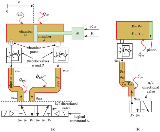
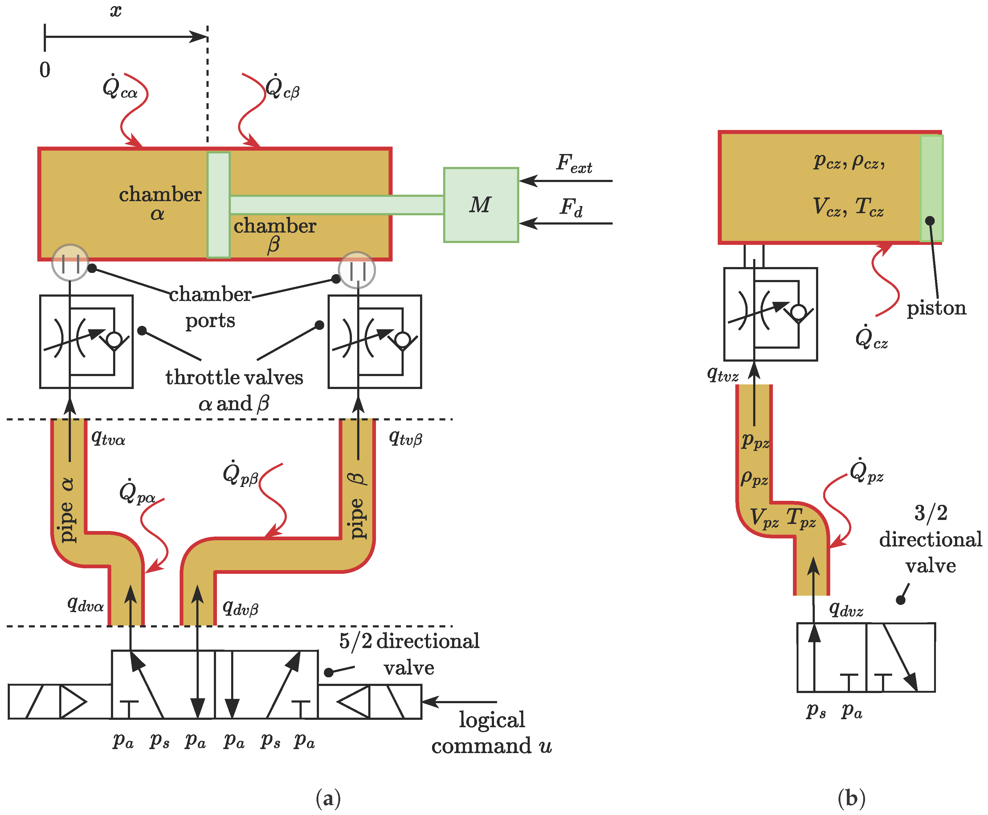
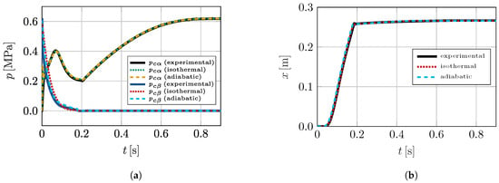
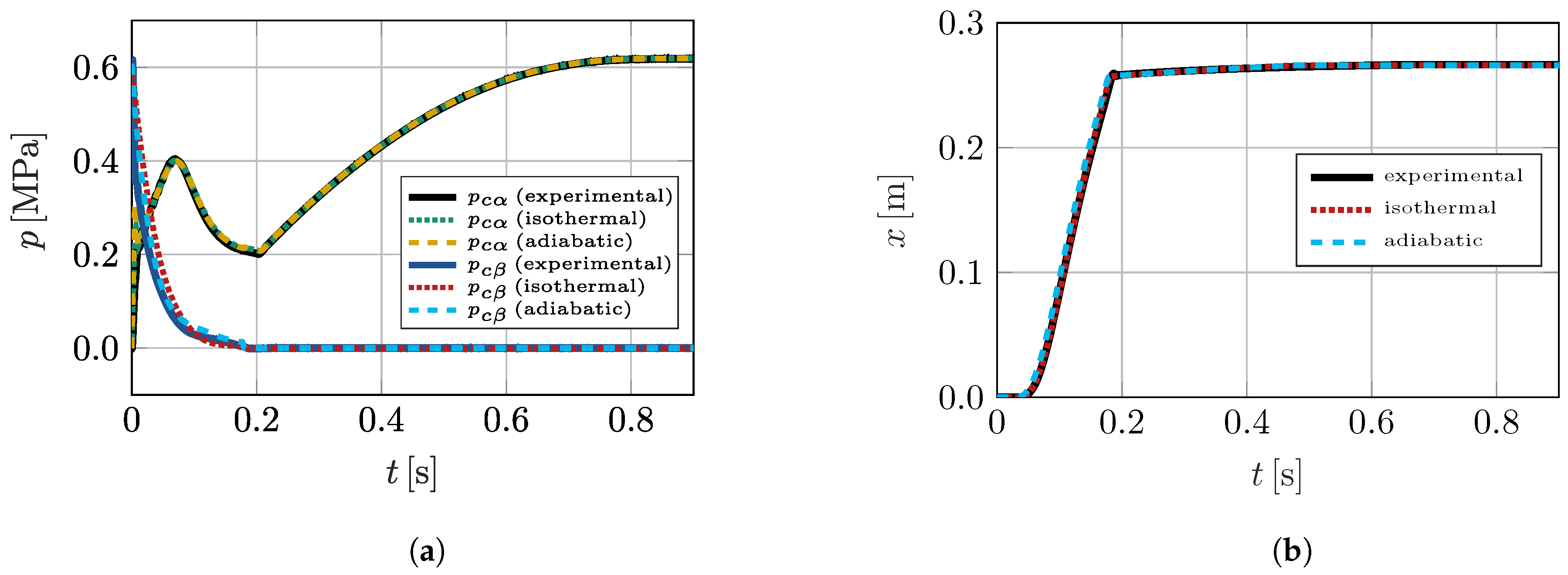
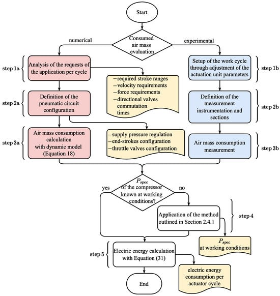
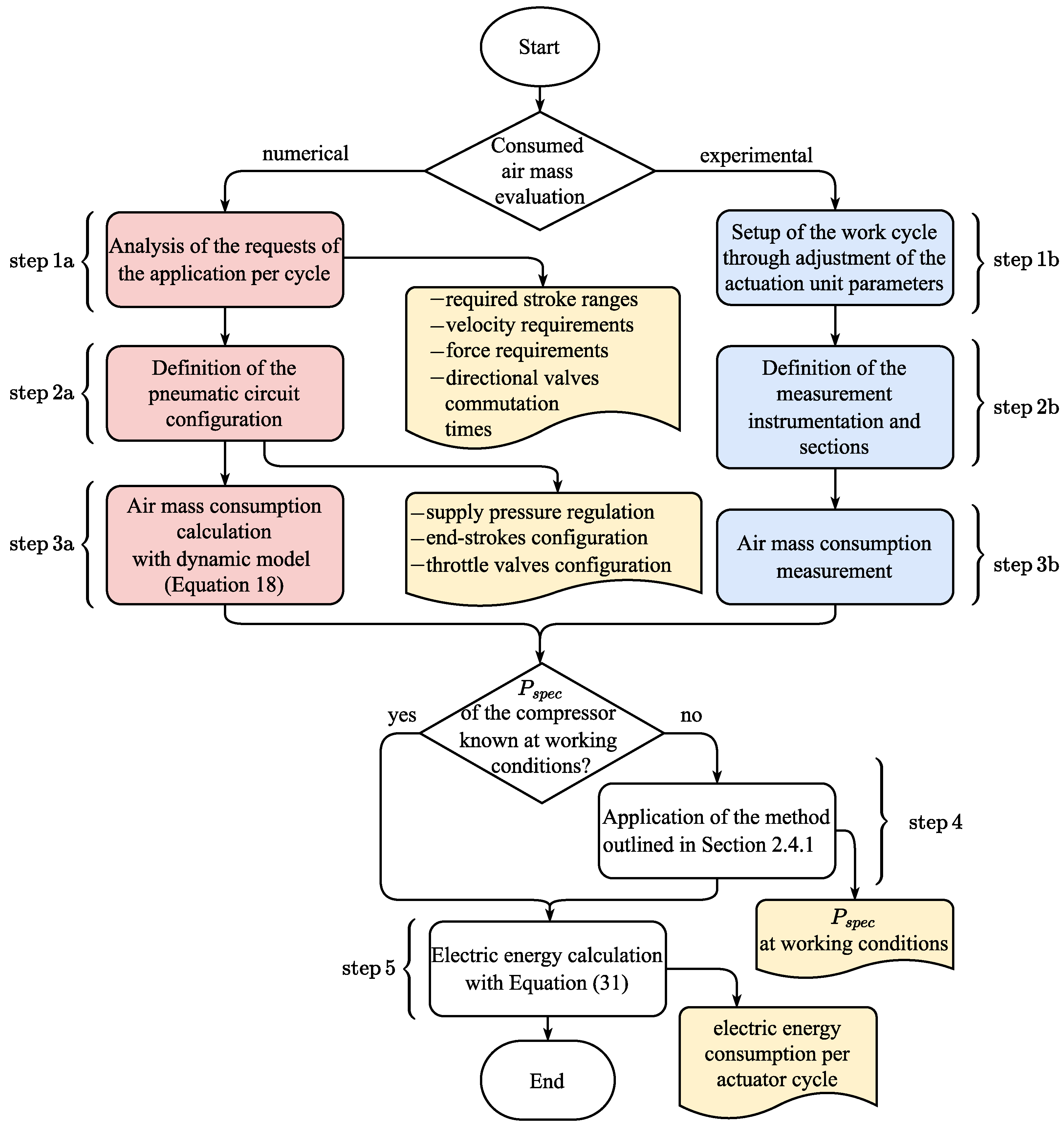
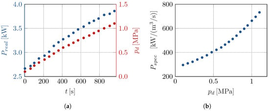
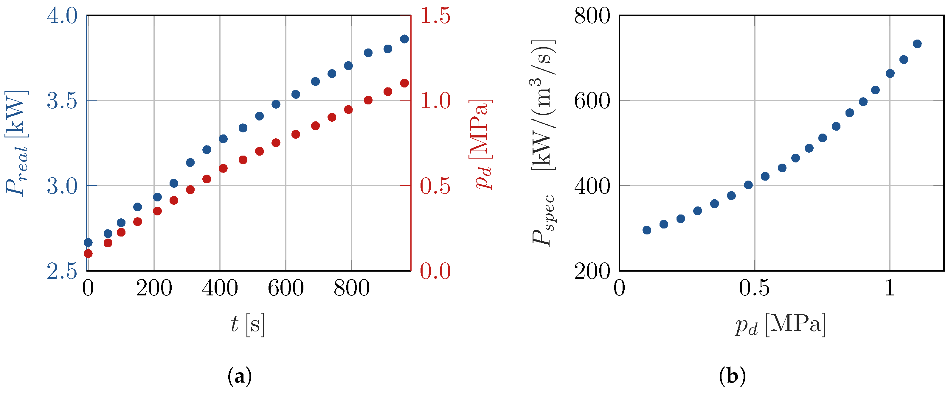
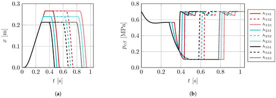
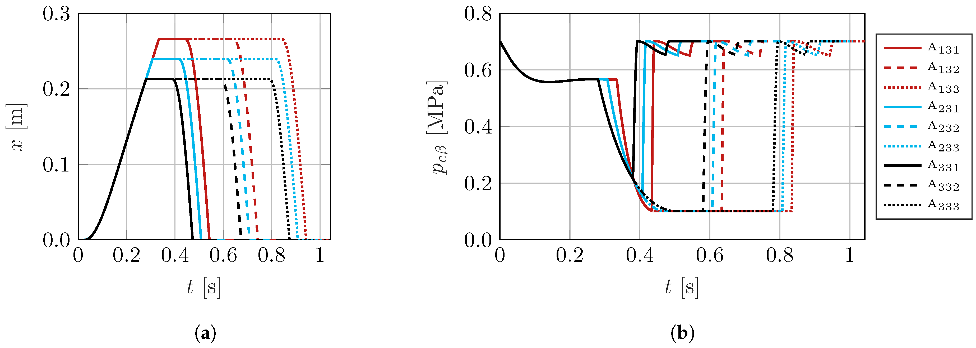
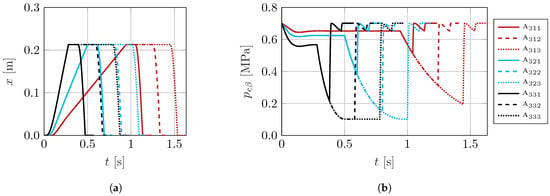
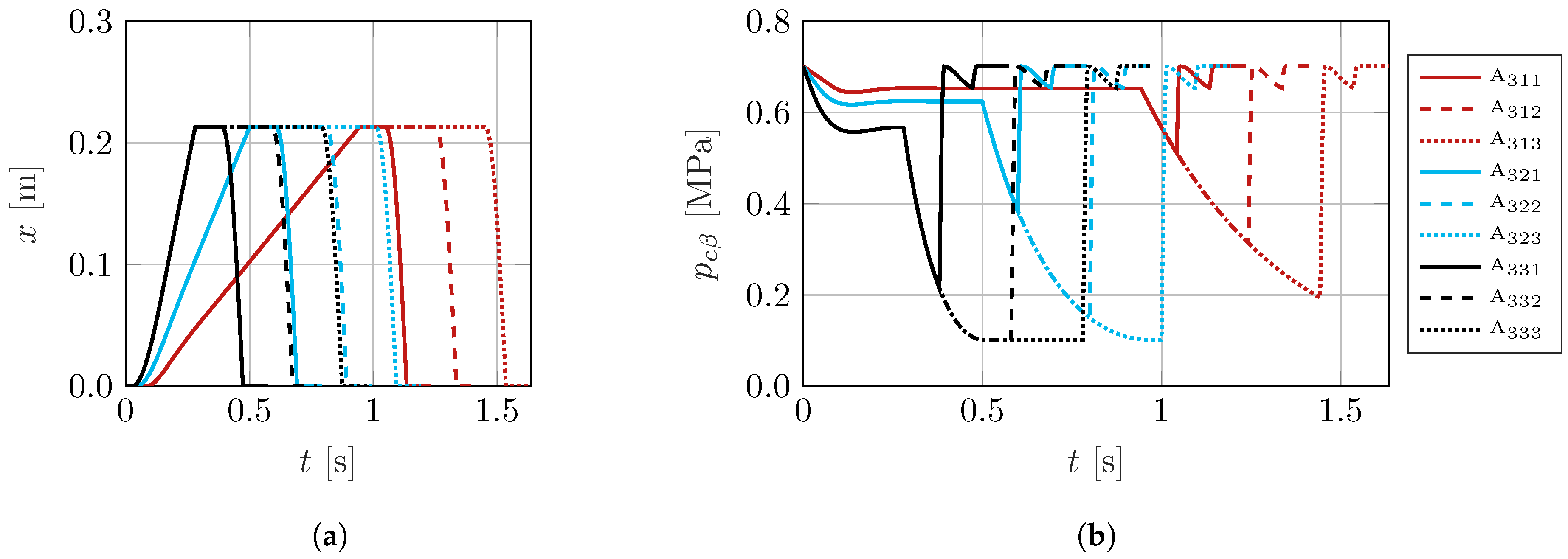
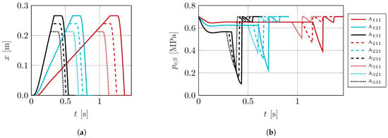
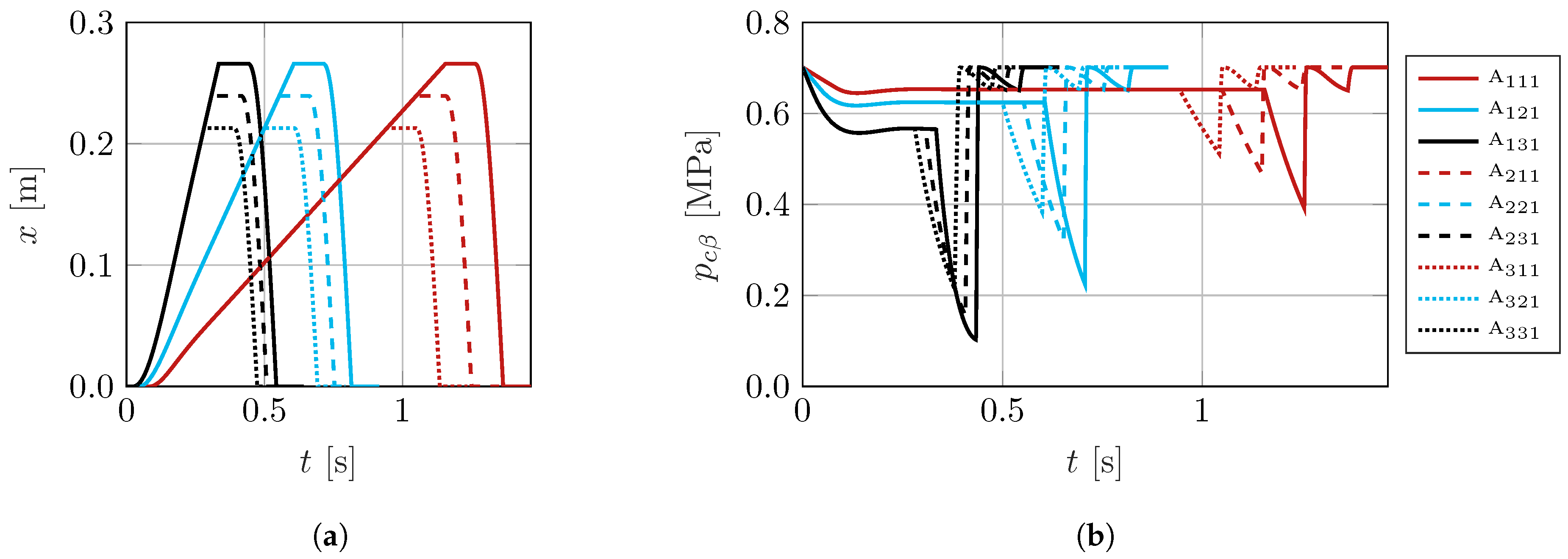
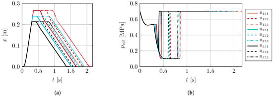
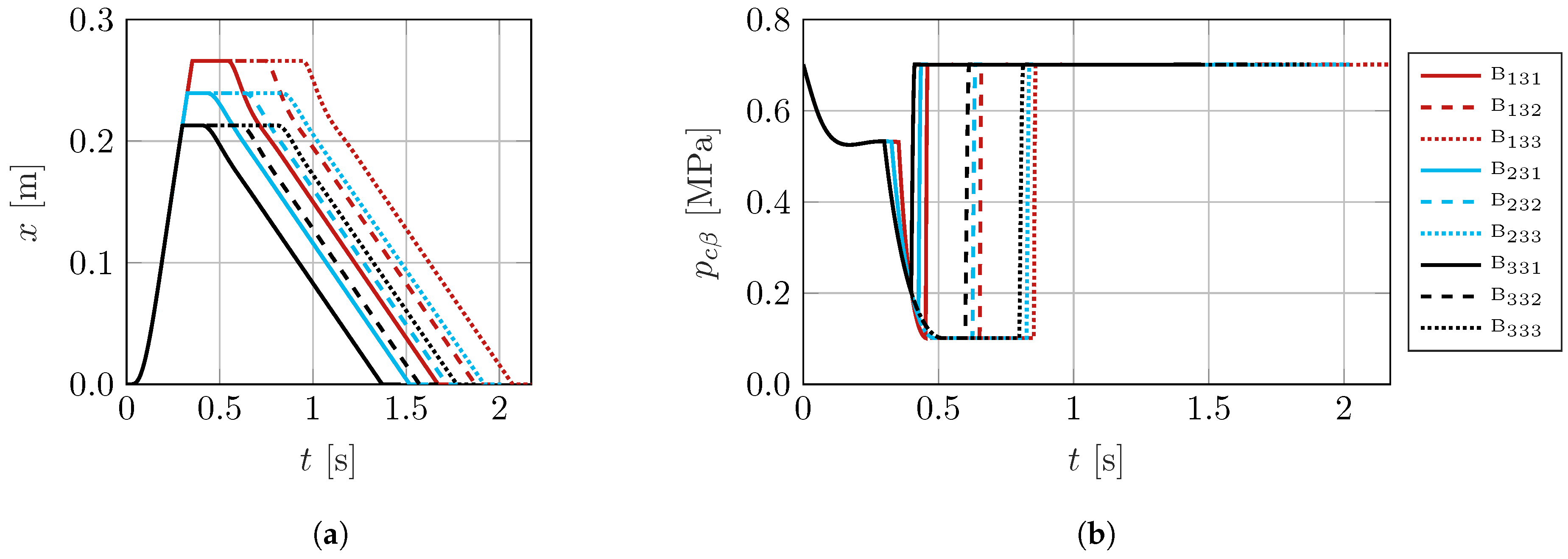
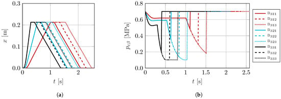
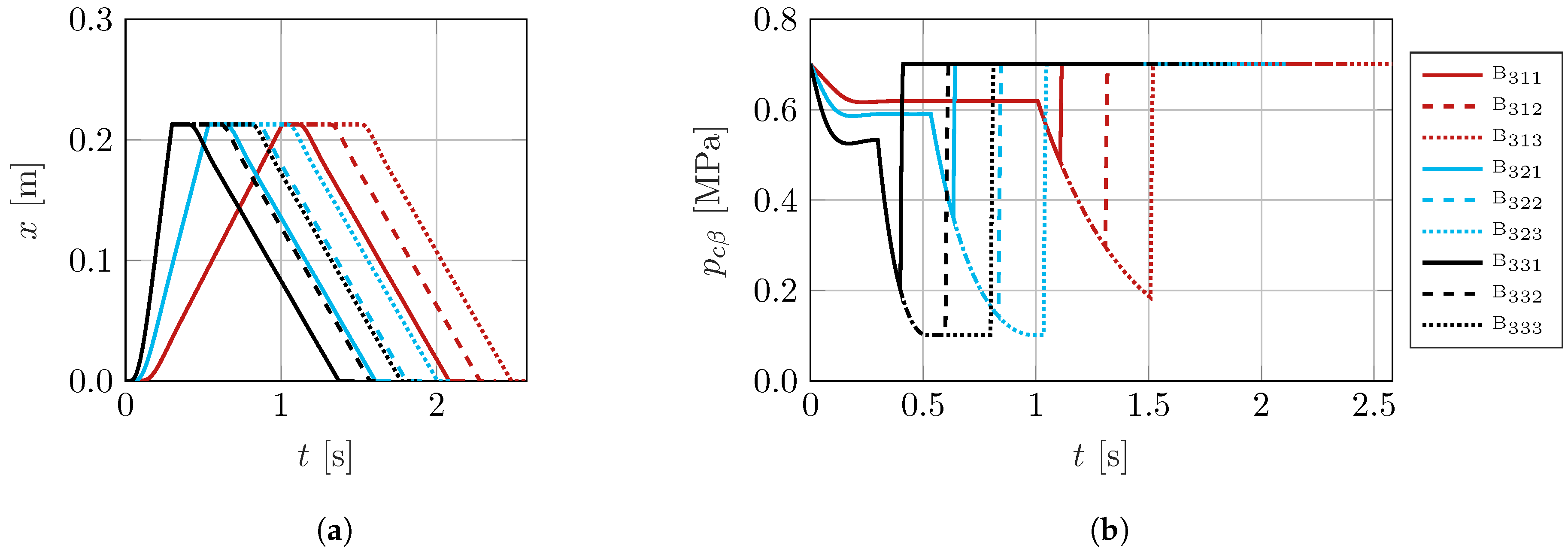
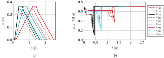
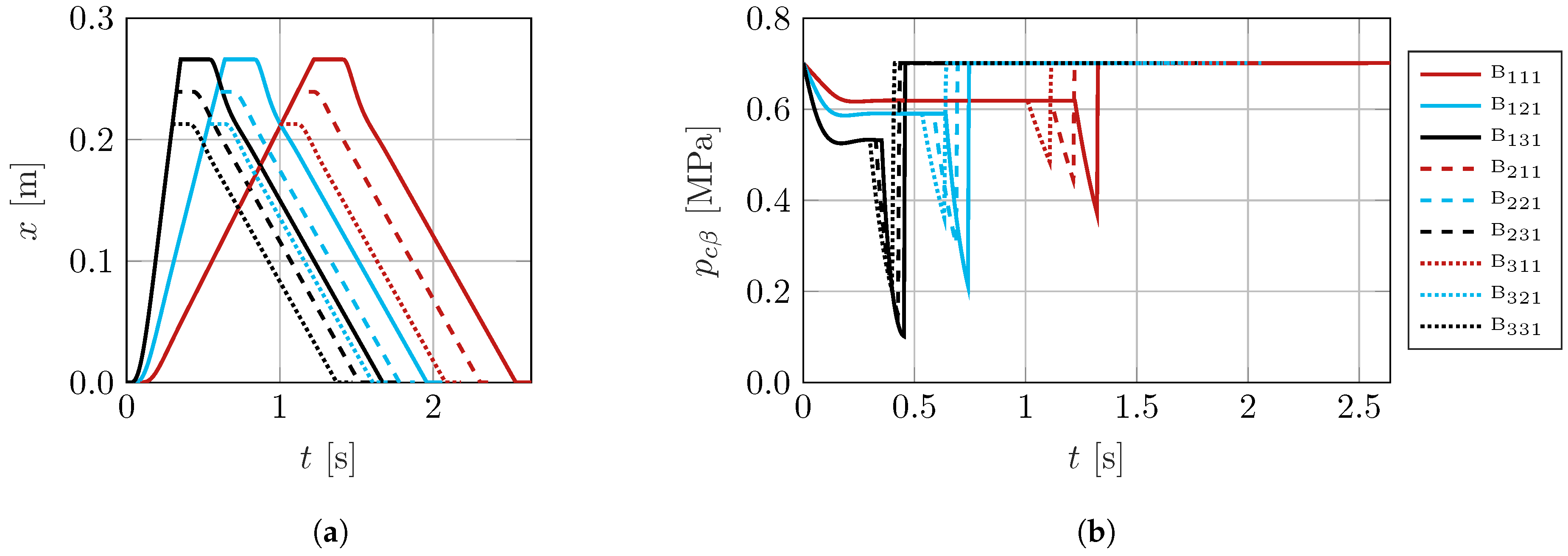
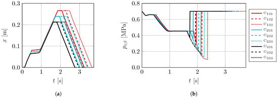
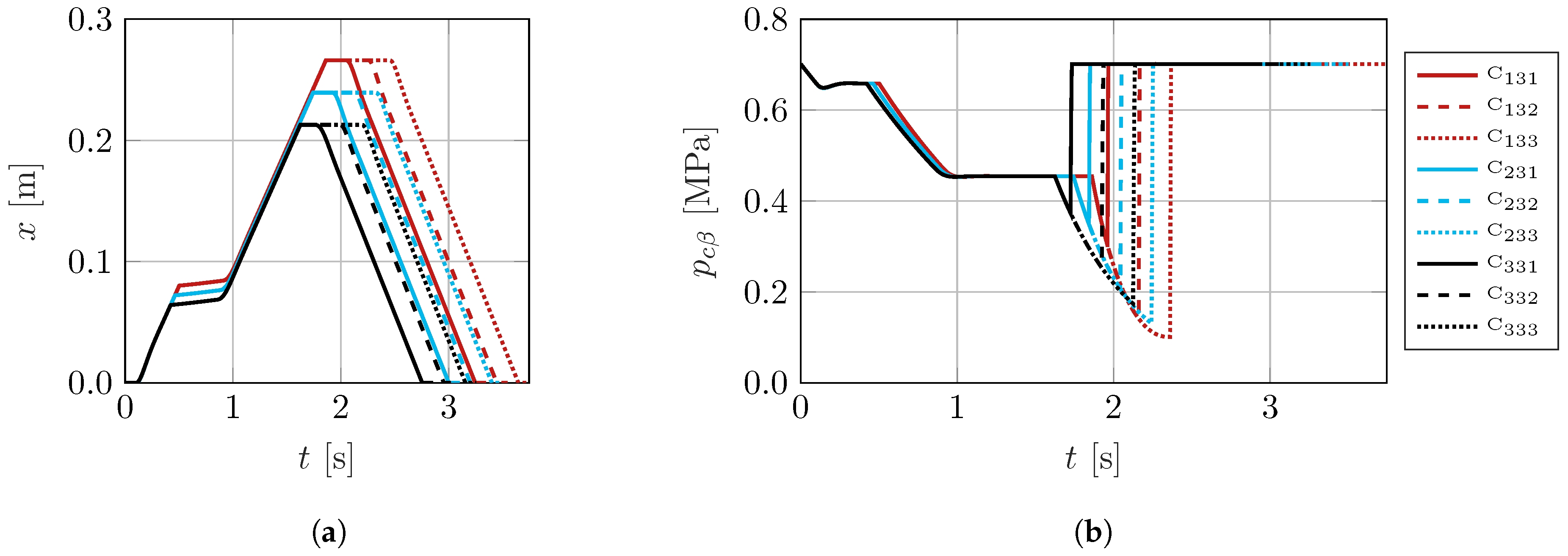
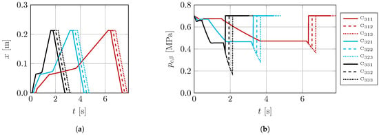
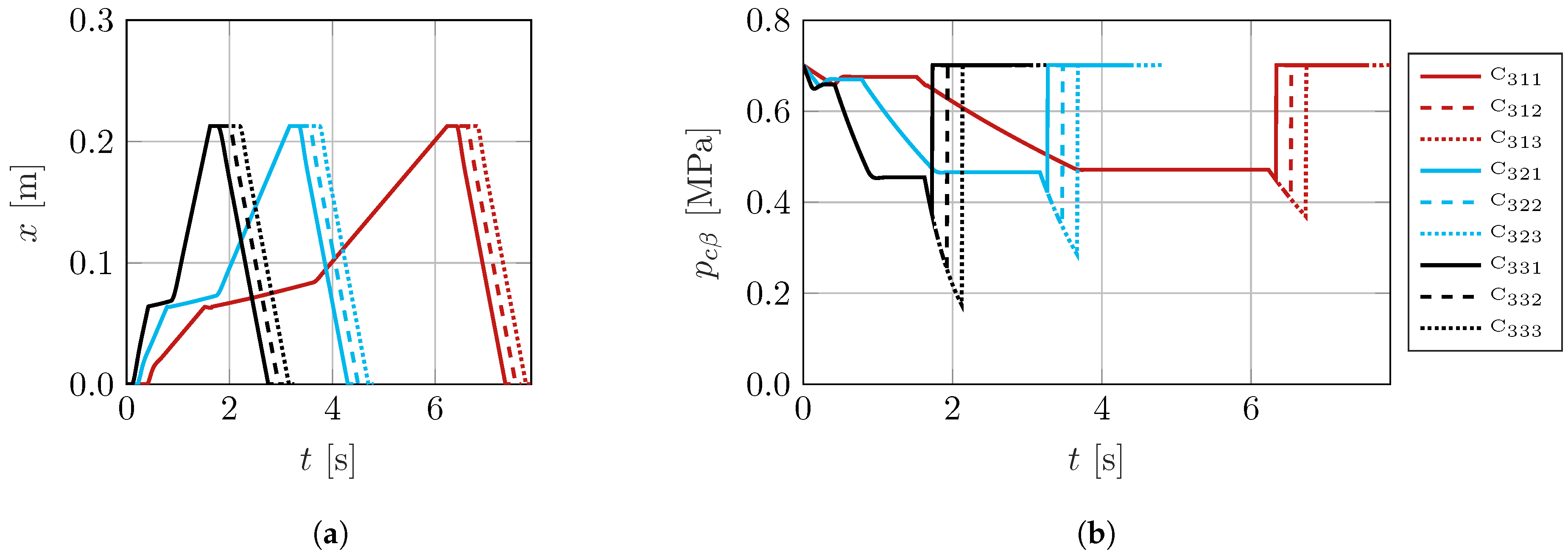
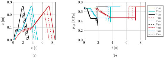
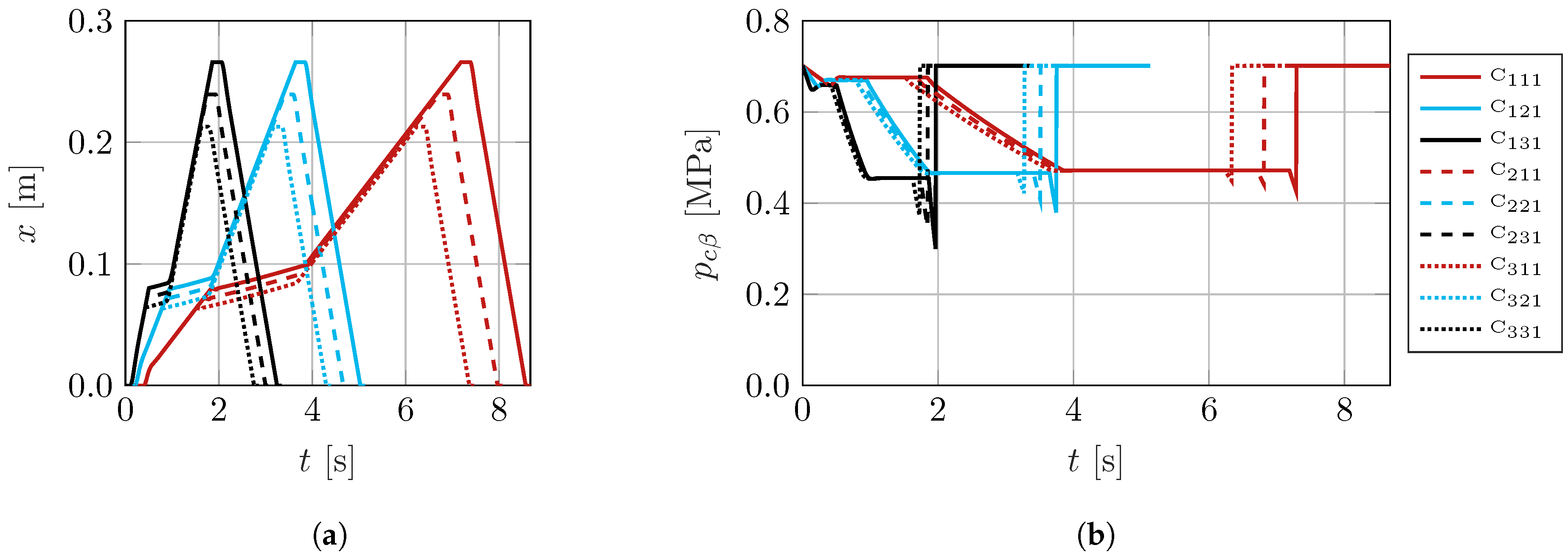
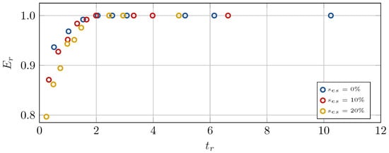
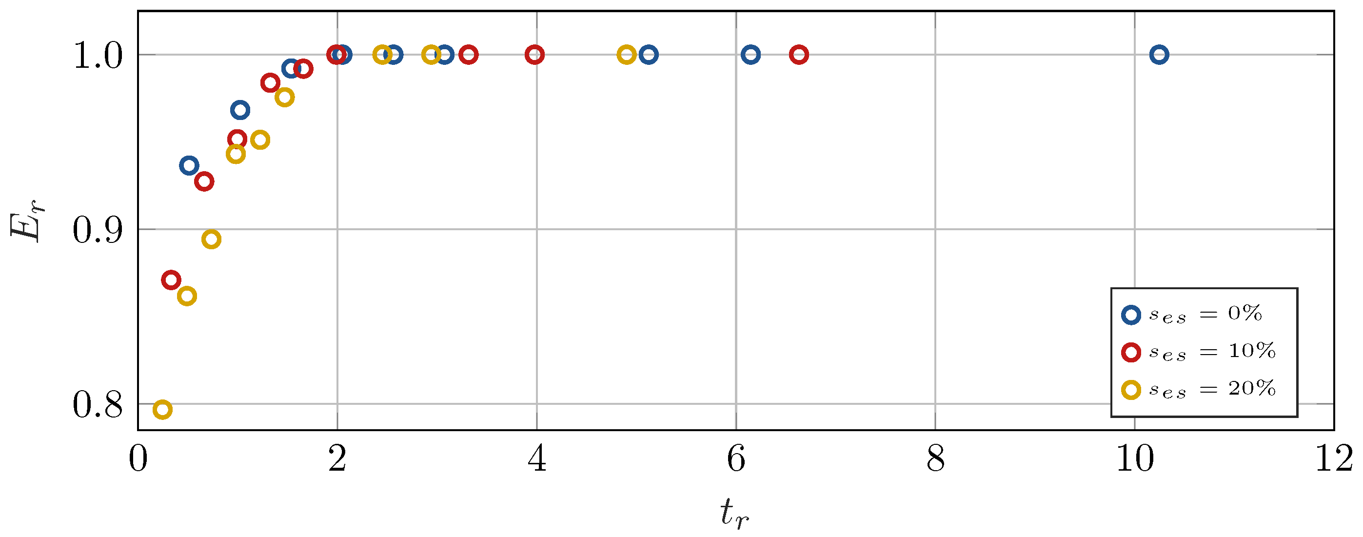
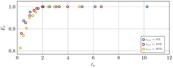
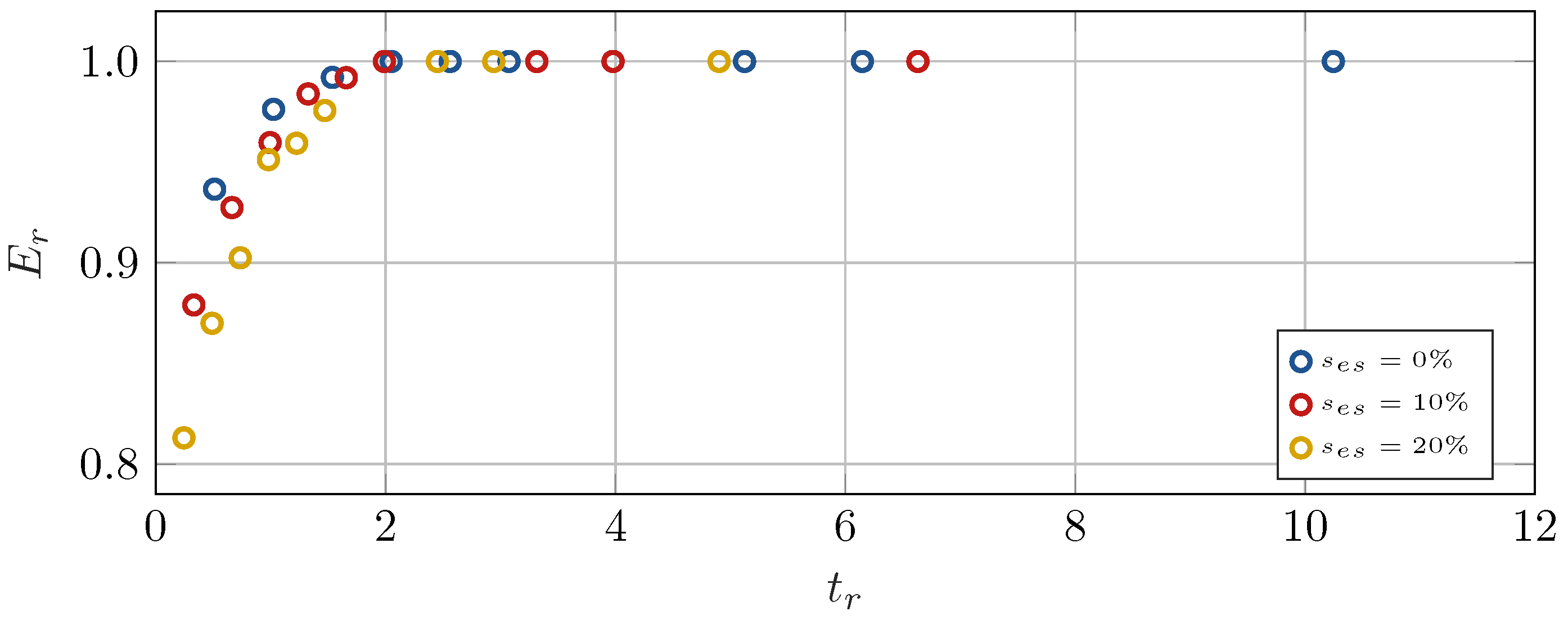
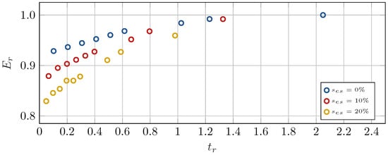
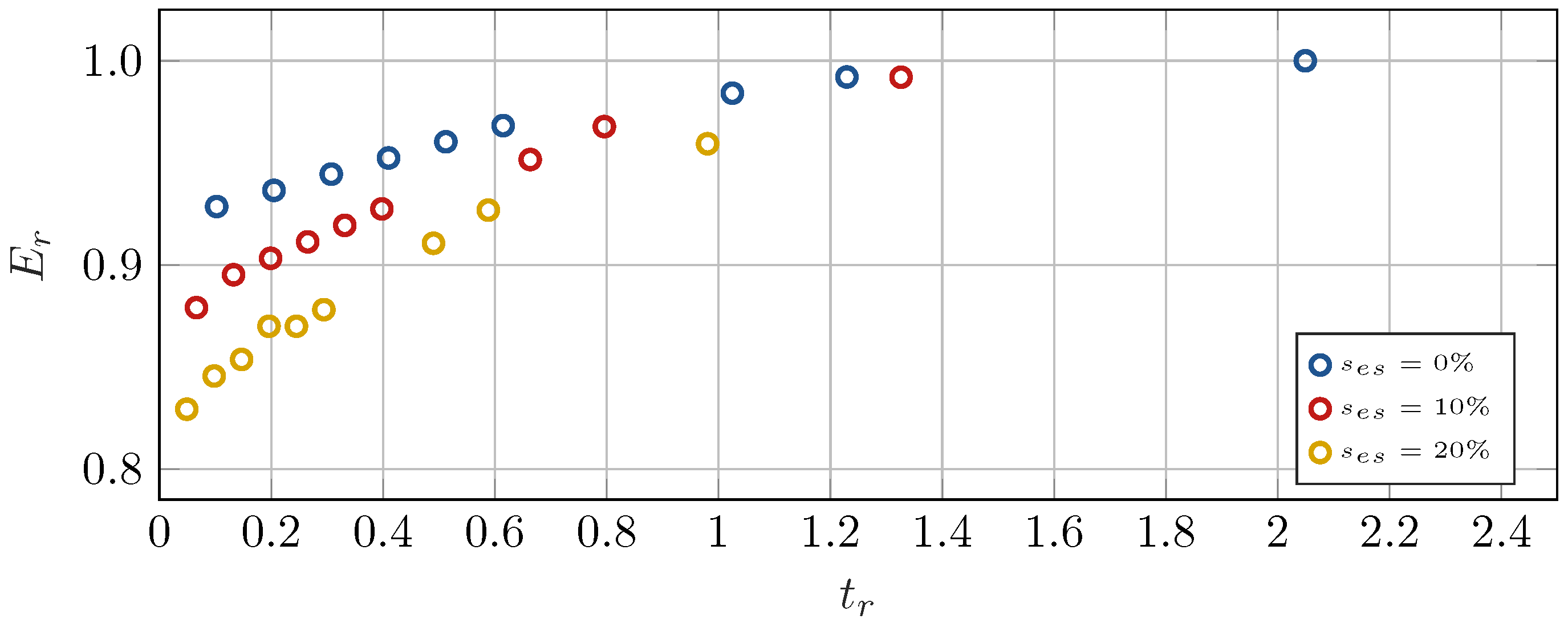
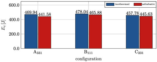
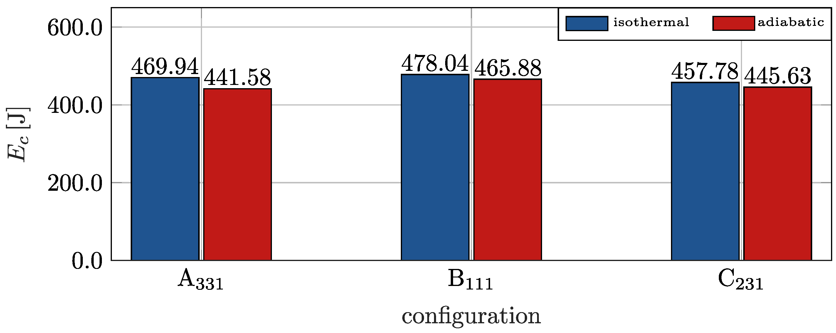
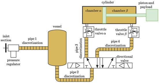
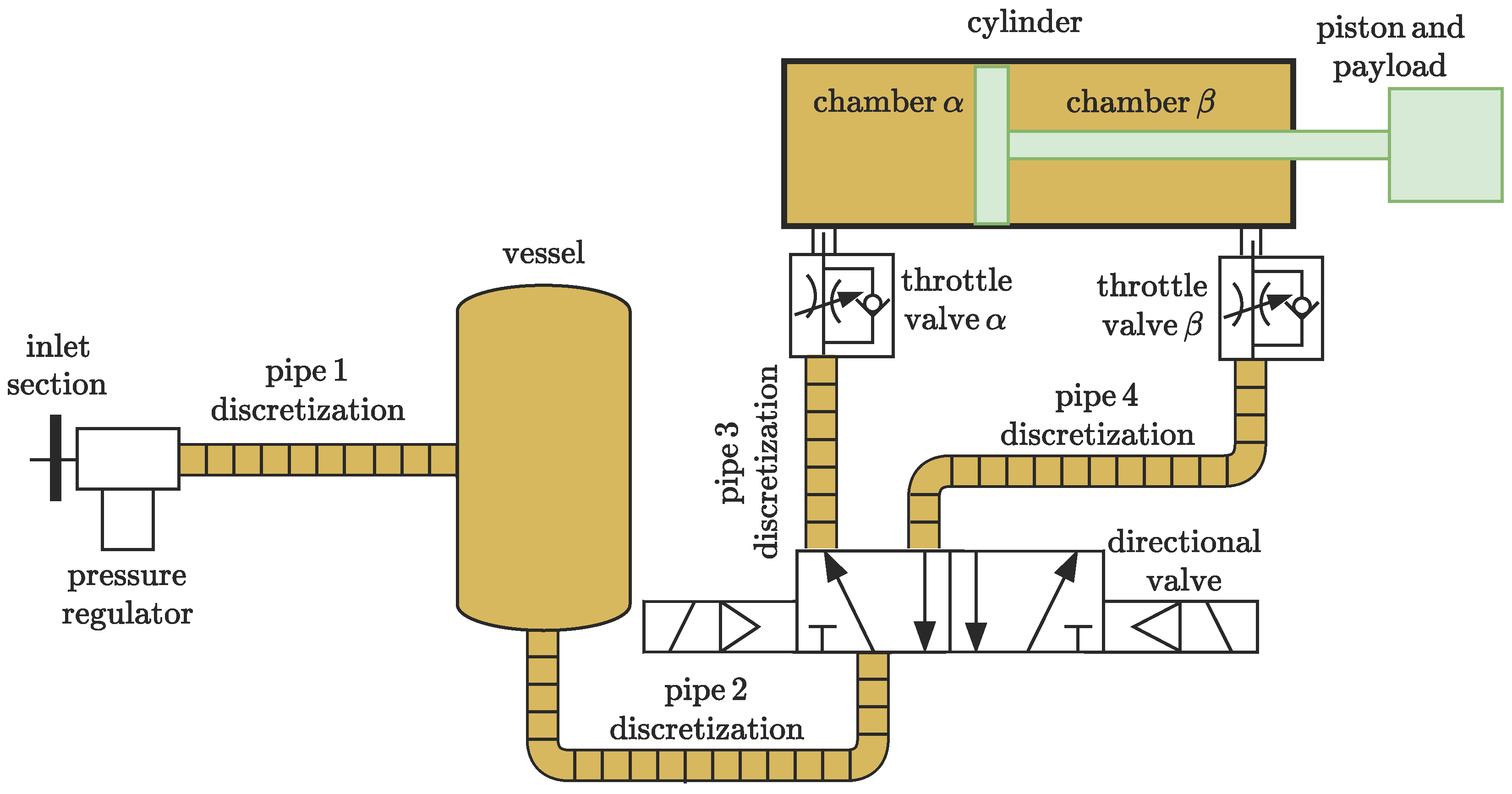
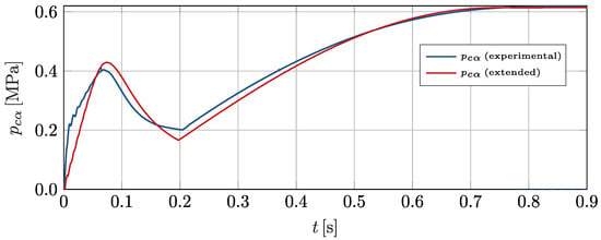
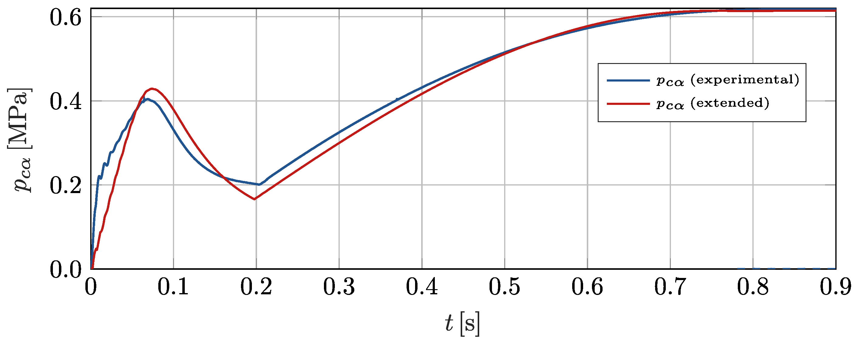
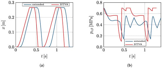
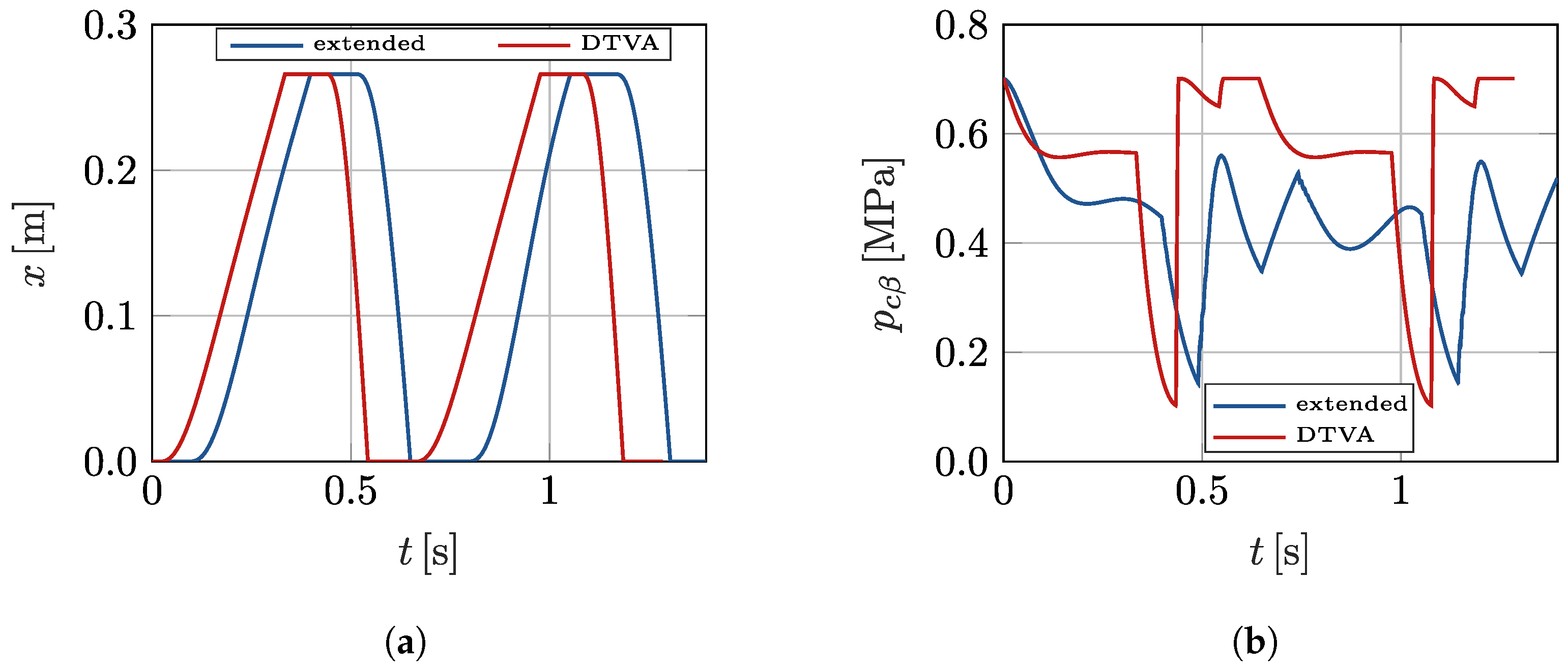
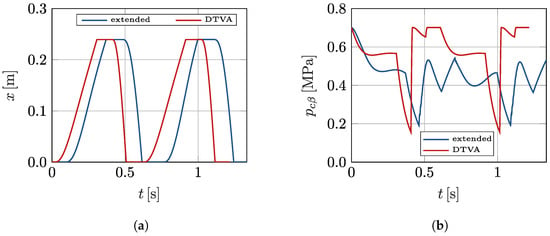
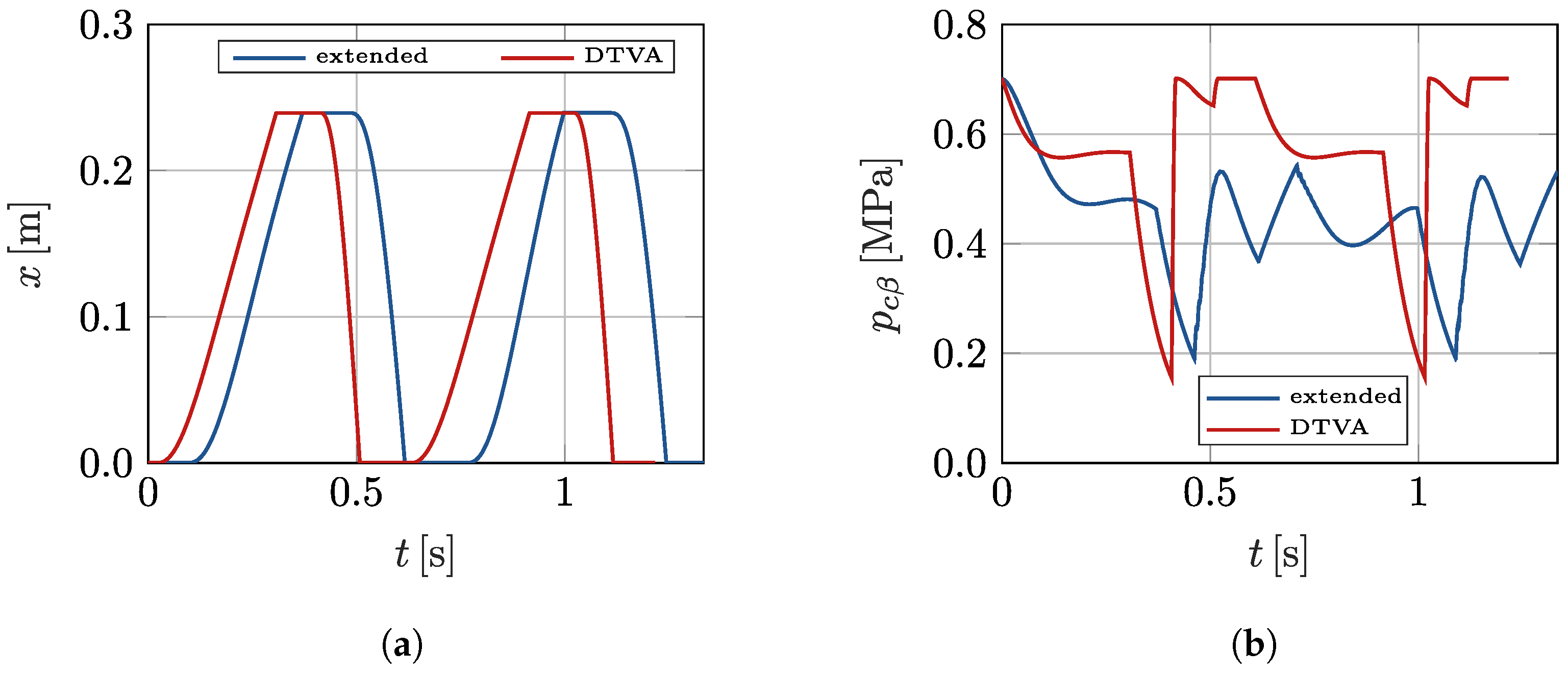
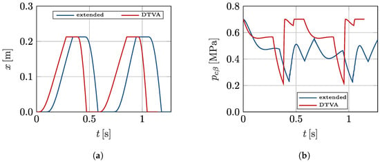
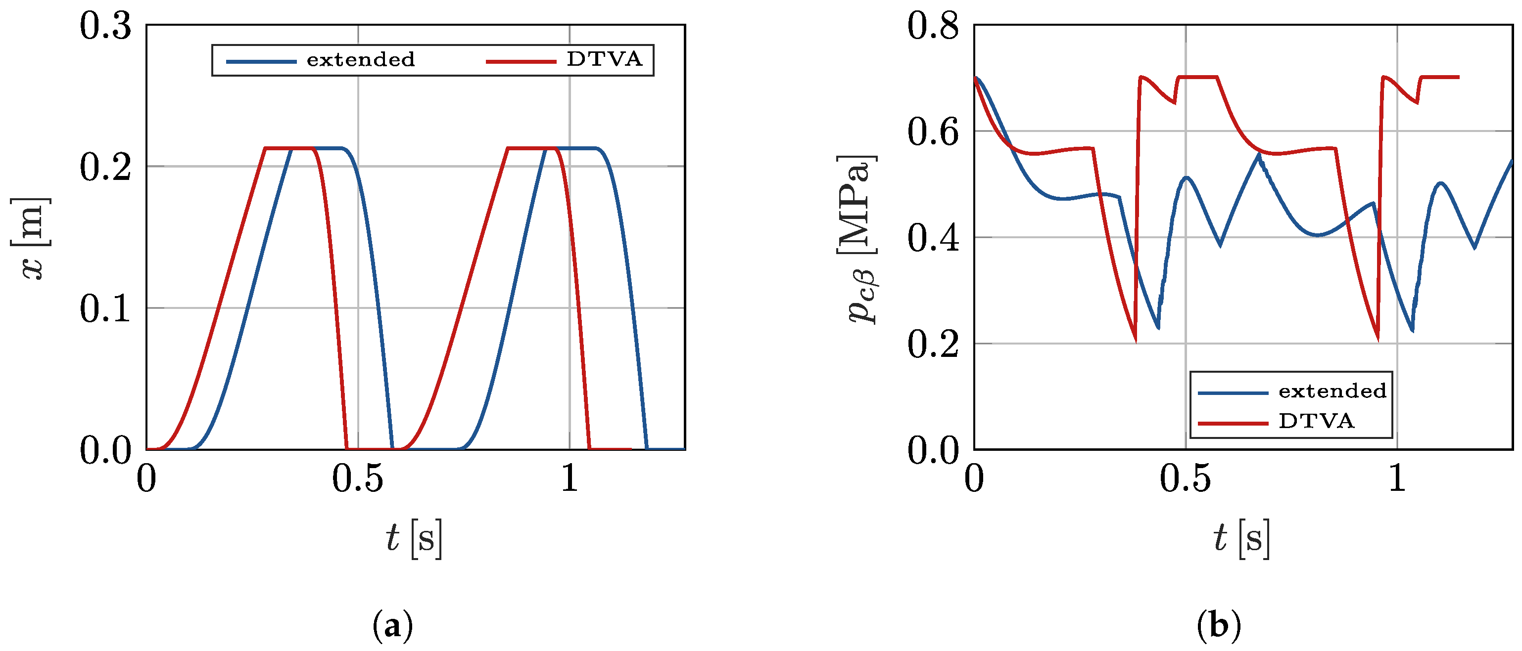

Disclaimer/Publisher’s Note: The statements, opinions and data contained in all publications are solely those of the individual author(s) and contributor(s) and not of MDPI and/or the editor(s). MDPI and/or the editor(s) disclaim responsibility for any injury to people or property resulting from any ideas, methods, instructions or products referred to in the content. |
© 2026 by the authors. Licensee MDPI, Basel, Switzerland. This article is an open access article distributed under the terms and conditions of the Creative Commons Attribution (CC BY) license.