Autonomous Vehicle Front Steering Control Computation Saving

Abstract

In autonomous vehicle trajectory tracking, lane-keeping control often relies on high-order robust controllers designed with multiple performance requirements encoded via weighting functions. Such designs typically entail a significant computational cost that can overload processors already devoted to demanding tasks, such as computer vision. This work introduces an interlacing strategy for the implementation of a given robust state-space controller, with the aim of reducing its computational burden while preserving acceptable closed-loop behavior. The approach operates directly on a state-space realization and is extendable to high-order MIMO controllers, considering both diagonal (modal) and balanced realizations combined with different input–output update schemes. The method is illustrated through simulations under conditions representative of an automotive test-track circuit, indicating that substantial computational savings can be achieved at the expense of a moderate deterioration of the closed-loop response.

1. Introduction

The lateral guidance of autonomous vehicles critically relies on the precise regulation of the yaw angle, which is achieved by suitably actuating the steering system. The dynamic relationships between these variables are highly coupled, and the associated model parameters exhibit a marked dependence on operating conditions, in particular on the longitudinal velocity of the vehicle. Therefore, the resulting models are characterized by a high level of parametric uncertainty, which motivates the use of robust control methodologies. Such methodologies typically yield high-order controllers whose poles are associated with dynamics evolving on clearly separated time scales, which poses significant challenges for their implementation in computationally constrained embedded platforms.

In this context, planar single-track vehicle models have been extensively employed for lateral control design, as they provide a convenient compromise between fidelity and complexity. Zhang et al. [1] proposed an active front-steering controller based on such a model within a Quantitative Feedback Theory (QFT) framework and further developed this approach in [2]. Rajamani [3] systematically developed planar vehicle dynamics models for lane-keeping and yaw-stability control applications. Other relevant contributions include the combined linear active disturbance rejection control and QFT strategy proposed by Chu et al. [4], the LPV/H∞ path-tracking design by Hang et al. [5], and the comparative evaluation of lateral control methods by Artuñedo et al. [6]. Application-specific system identification approaches for model-based control in self-driving cars have also been explored by Salt Ducaju et al. [7]. These formulations provide the main references for the vehicle model adopted in the present work.

The primary objective of this work is to propose an implementation strategy for the high-order robust controllers that naturally arise in this setting, achieving a significant reduction in computational burden. Two classical approaches can be considered for this purpose: reducing the controller order or increasing the sampling period. Order reduction is based on discarding the least influential dynamics, whereas an increase in the sampling period degrades the closed-loop response; in both cases, performance inevitably deteriorates.

In this regard, Bhattacharya and Balas [8] established a framework for the implementation of LTI controllers in computationally constrained environments by combining model reduction techniques with anytime control strategies, whereby controllers of different complexity are scheduled according to the computation time available. An alternative intermediate solution is provided by controllers implemented using interlacing techniques, as discussed by Salt [9], Wu and Tomizuka [10], and Salt and Tomizuka [11]. These approaches distribute the computation of the control action over several slow periods, phase-shifted with respect to each fast-sampling period, without discarding any of the controller dynamics. In this way, the complete structure of the controller is preserved while the computational load required at each fast period is substantially reduced. Previous contributions have addressed this problem mainly in transfer-function form for SISO controllers.

While this approach has proved effective in several applications, its direct extension to higher-order robust controllers and MIMO systems is not straightforward, particularly when multiple or complex-conjugate poles are present. In parallel, recent works on trajectory- and path-tracking control for autonomous vehicles by Al-Saedi and Al-Bawi [12], Lin et al. [13], Lee and Jeong [14], Lelkó et al. [15], and Park et al. [16] further motivate the need for implementation strategies that reduce the computational burden of high-performance controllers without significantly degrading their closed-loop behavior.

The present work revisits this idea in the context of autonomous vehicle lateral control and extends it to high-order robust controllers represented in state space. Rather than introducing a new multirate control theory, the focus is on a practical implementation/decomposition strategy for a given μ-synthesis controller, aiming to balance computational efficiency and closed-loop behavior. The interlacing procedure is formulated directly on a state-space realization of the controller, which enables its extension to MIMO systems of arbitrary dimension and allows the systematic study of different structural configurations and update schemes.

The main contributions of this work are as follows:

• An interlacing-based implementation strategy is proposed, formulated directly on a state space representation of a given high-order robust controller and enabling its application to MIMO systems of arbitrary dimension.
• Alternative interlacing structures are systematically analyzed, combining diagonal (modal) and balanced realizations with different input–output update schemes, and their impact on closed loop behavior and implementation complexity is discussed.
• It is illustrated how suitable choices of the interlacing order and subsystem allocation can provide substantial reductions in computational load at the expense of a moderate deterioration of the closed-loop response under conditions representative of an automotive test track circuit.

The remainder of the paper is organized as follows. Section 2 presents the lateral vehicle model and the μ-synthesis controller that serves as the starting point for the study. Section 3 analyzes the controller in its diagonal modal form to identify suitable groupings of dynamics for subsequent partitioning. Section 4 addresses the implementation of the interlacing controller, considering different structural configurations and criteria for allocating the controller dynamics among fast and slow components. Section 5 presents a comparative assessment of the resulting closed-loop behaviors. Finally, Section 6 summarizes the main conclusions and outlines potential directions for future research.

2. Vehicle Model and Controller Design

In this section, the dynamic vehicle model employed for the design of the lateral guidance controller is presented, together with the reference framework associated with the road model. Based on this model, a high-order robust controller is designed, which will serve as the starting point for the subsequent application of the interlacing techniques.

2.1. Lateral Vehicle Model

The dynamic vehicle model used in this work is based on the classical planar vehicle formulation developed for advanced lateral guidance and stability control applications. Under the usual assumptions of small vertical accelerations and negligible roll and pitch angles, the vehicle dynamics in the horizontal plane are represented by a single-track model (bicycle or single-track model), in which the two front tires are grouped into an equivalent wheel and the same applies to the rear tires [1,3]. Other dynamic models suitable for autonomous vehicle control, including application-specific system identification approaches for self-driving cars that account for varying road and driving conditions, can also be found in [7].

In this model, the lateral motion is described in terms of the longitudinal velocity of the center of gravity, the lateral velocity, the yaw rate and, when lane-keeping is required, the lateral position and orientation errors with respect to the reference trajectory. The lateral forces on the front and rear axles are modeled in the linear operating region of the tire, relating each force to its corresponding slip angle through the total cornering stiffnesses of the front and rear axles. This leads to a low-order state-space representation suitable for the design of robust controllers.

This formulation is consistent with the lateral dynamics models employed by Rajamani [3] in the context of lane-keeping and yaw stability control, and with the simplified planar model used by Zhang et al. for the design of QFT controllers for active front-axle steering [1]. In both cases, the single-track model provides an adequate compromise between simplicity and the ability to capture the essential effects of lateral vehicle dynamics, allowing explicit consideration of the influence of longitudinal velocity, mass distribution and lateral tire stiffness characteristics on the guidance behavior.

The equilibrium of forces and moments in the horizontal plane, neglecting roll and pitch motions, yields the following equations of motion:

$$\{\begin{array}{c}m{a}_y=F_{y,f}\cos \delta +F_{y,r}\\ I_z\dot{\gamma }=a{F}_{y,f}\cos \delta -b{F}_{y,r}\end{array}$$

where $m$ is the vehicle mass, $a_y$ is the lateral acceleration, $F_{y,f}$ and $F_{y,r}$ are the lateral forces on the front and rear axles, $\delta$ is the steering angle of the front wheels, $I_z$ is the yaw moment of inertia, $\gamma$ is the yaw rate, and $a$ and $b$ are the distances from the center of gravity to the front and rear axles, respectively.

In the linear operating region of the tire, the lateral forces are related to the slip angles by:

$$F_{y,f}=C_{\alpha ,f}{\alpha }_f$$

$$F_{y,r}=C_{\alpha ,r}{\alpha }_r$$

where $C_{\alpha ,f}$ and $C_{\alpha ,r}$ are the total cornering stiffnesses of the front and rear axles, and ${\alpha }_f$ and ${\alpha }_r$ are the corresponding slip angles. Under the small-angle approximation, the slip angles can be expressed as functions of the center-of-gravity velocities and the yaw rate:

$${\alpha }_f=\delta -{\displaystyle \frac{u_y+a\gamma }{u_x}}$$

$${\alpha }_r=-{\displaystyle \frac{u_y-b\gamma }{u_x}}$$

where $u_x$ and $u_y$ denote the longitudinal and lateral components of the center-of-gravity velocity.

Assuming a practically constant longitudinal velocity ($u_x\approx V_x$) and defining the sideslip angle of the center of gravity as $\beta =\mathrm{a}\mathrm{r}\mathrm{c}\mathrm{t}\mathrm{a}\mathrm{n} (u_y/u_x)\approx u_y/V_x$, the model can be written in state-space form as:

$$\left[\begin{array}{c}\dot{\beta }\\ \dot{\gamma }\end{array}\right]=\left[\begin{array}{cc}-{\displaystyle \frac{C_{\alpha ,f}+C_{\alpha ,r}}{m{V}_x}}& -1-{\displaystyle \frac{C_{\alpha ,r}·b-C_{\alpha ,f}·a}{m·V_x^2}}\\ -{\displaystyle \frac{C_{\alpha ,r}·b-C_{\alpha ,f}·a}{I_z}}& -{\displaystyle \frac{C_{\alpha ,f}·a^2+C_{\alpha ,r}·b^2}{I_z·V_x}}\end{array}\right]· \left[\begin{array}{c}\beta \\ \gamma \end{array}\right]+\left[\begin{array}{c}{\displaystyle \frac{C_{\alpha ,f}}{m·V_x}}\\ {\displaystyle \frac{C_{\alpha ,f}·a}{I_z}}\end{array}\right]·\delta$$

For trajectory-tracking control, the previous model is extended by including the lateral position error ($e_y$) and the orientation error (${\psi }_e$) with respect to the reference trajectory defined by the road. The dynamics of these errors are given by:

$${\dot{e}}_y=V_x·\sin {\psi }_e+u_y·\cos {\psi }_e\approx V_x·{\psi }_e+u_y$$

$${\dot{\psi }}_e=\gamma -{\gamma }_{des}$$

where ${\gamma }_{des}$ is the desired yaw rate, computed from the curvature of the reference trajectory as ${\gamma }_{des}=V_x/R$, with $R$ denoting the lane curvature radius.

The complete state-space model for lateral guidance control can then be written as:

$$\dot{x}=A·x+B_1·\delta +B_2·{\gamma }_{des}$$

with the state vector $x=[e_y,{\psi }_e,\beta ,\gamma {]}^T$, where the matrices $A$, $B_1$ and $B_2$ incorporate the vehicle parameters mentioned above.

The parameter values used in this work, representative of a compact passenger car under urban driving conditions, are as follows: mass $m=995 \mathrm{k}\mathrm{g}$, yaw moment of inertia $I_z=1760 \mathrm{k}\mathrm{g}·{\mathrm{m}}^2$, distances $a=1.233 \mathrm{m}$ and $b=1.327 \mathrm{m}$ (wheelbase $l=2.56 \mathrm{m}$), and cornering stiffnesses $C_{\alpha ,f}=\mathrm{41,000} \mathrm{N}/\mathrm{r}\mathrm{a}\mathrm{d}$ and $C_{\alpha ,r}=\mathrm{47,000} \mathrm{N}/\mathrm{r}\mathrm{a}\mathrm{d}$.

For robust controller design, the steering angle $\delta$ is taken as the control input and the yaw rate $\gamma$ as the output, since the latter is the most relevant variable from the viewpoint of lateral stability control. The transfer function of the continuous-time process relating yaw rate to steering angle is obtained directly from the lateral model, yielding an expression of the form

$${\displaystyle \frac{\gamma \left(s\right)}{\delta \left(s\right)}}={\displaystyle \frac{m{V}_{x}a{C}_{\alpha ,f}s+l{C}_{\alpha ,f}{C}_{\alpha ,r}}{m{V}_x{I}_z{s}^2+\left[I_z(C_{\alpha ,f}+C_{\alpha ,r})+m(a^2{C}_{\alpha ,f}+b^2{C}_{\alpha ,r})\right]s+C_{\alpha ,f}{C}_{\alpha ,r}{l}^2\left[1+\frac{m{V}_x(b{C}_{\alpha ,r}-a{C}_{\alpha ,f})}{C_{\alpha ,f}^2{l}^2}\right]}}$$

where $l=a+b$ denotes the wheelbase. This transfer function depends strongly on the longitudinal velocity $V_x$, which in urban operation typically varies in the range from 4 to 20 m/s. To explicitly account for this parametric uncertainty in the controller design, $V_x$ is modeled as an uncertain parameter with nominal value 10 m/s and variation range $V_x\in [4,20]$ m/s. This leads to the following nominal plant:

$${\displaystyle \frac{\gamma \left(s\right)}{\delta \left(s\right)}}={\displaystyle \frac{28.72s+281.7}{s^2+17.09s+72.88}}$$

2.2. Robust Controller Design

Authors such as Artuñedo et al. [6], Rajamani [3], Zhang et al. [2], and Hang et al. [5] have addressed lateral vehicle control from different perspectives: QFT, H∞, and μ-synthesis. The use of these techniques yields high-order controllers. Based on the nominal model described above and considering the presence of uncertainties in the longitudinal velocity of the vehicle, a robust controller is designed by means of μ-synthesis techniques. The design imposes specifications on the tracking of the reference yaw rate and on robustness against parametric variations within the considered velocity range, which results in a controller of relatively high order.

The μ-synthesis controller designed for this application is a 13th-order system and has been tuned to guarantee the required stability and tracking specifications for variations of $V_x$ in the interval from 4 to 20 m/s. The controller can be expressed in pole–zero form as:

$$\begin{array}{c}{G}_R\left(s\right)={\displaystyle \frac{110.68\left(s+13.17\right)\left(s+8.985\right)\left(s+8.032\right)\left(s+6\right)\left(s+3.161\right)\left(s+2.145\right)}{\left(s+230\right)\left(s+9.905\right)\left(s+3.494\right)\left(s+2.811\right)\left(s+0.003\right)\left(s^2+3.148s+12.78\right)}}\\ ·{\displaystyle \frac{\left(s^2+ 7.487s+24.04\right)\left(s^2+41.14s+574\right)\left(s^2+76.68s+1902\right)}{\left(s^2+20.23s+117.8\right)\left(s^2+42.53s+640.3\right)\left(s^2+77.02s+1943\right)}}\end{array}$$

This controller is subsequently discretized with a sampling period $T=10 \mathrm{m}\mathrm{s}$, yielding a state-space realization that will serve as the basis for the modal analysis and the subsequent interlacing decomposition developed in the following sections. To validate the interlaced controllers, a unit-step reference is considered.

3. Controller Analysis

Several authors, including Salt [9], Wu and Tomizuka [10], and Salt and Tomizuka [11], have addressed the implementation of interlaced controllers expressed in transfer-function form, whose dynamics can be separated by means of partial-fraction expansion. For the case of real poles, the controller can be written as:

$$u\left(z\right)=G_{Reg}\left(z\right)·e\left(z\right)=\left(\sum _{i=1}^n{\displaystyle \frac{r_i}{z-p_i}}+d\right)·e(z)$$

where $p_i$ and $r_i$ denote the poles and residues of the controller, respectively, and $d$ represents the direct feedthrough term.

When multiple poles or complex-conjugate poles are present, they must be grouped, which entails additional computations, and the resulting groups of dynamics are then assigned to the different interlaced controllers. The same idea can be applied to the modal state-space form of the controller, with the additional advantage that multiple and complex-conjugate poles do not need to be explicitly grouped, since they naturally appear as Jordan blocks in the modal representation. Moreover, performing the analysis directly on the state-space controller allows the approach to be extended to the separation of dynamics in MIMO controllers.

This analysis can be carried out either for the controller designed in continuous time or for its discretized version with sampling period $T$, or even for a controller designed directly in discrete time. In any case, once the controller has been analysed, the number of parts into which its dynamics will be split must be decided. If the separation is performed in continuous time, each part must then be discretized with its corresponding sampling period, namely $T$ for the fast part and $N·T$ for the slow parts. If, instead, the separation is performed in discrete time, the fast part is kept at period $T$, whereas the slow parts must be resampled from the fast period $T$ to the slow period $N·T$.

In the application considered here, the starting point is a 13th-order controller designed using μ-synthesis techniques for a plant with parametric uncertainty. This controller is discretized with a sampling period $T=10 \mathrm{m}\mathrm{s}$. In its diagonal modal state-space form, given by:

$$\{\begin{array}{c} x_{Reg}\left(k+1\right)=\left[\begin{array}{cccc}{A}_1& 0& \cdots & 0\\ 0& A_2& 0& ⋮\\ ⋮& ⋮& \ddots & 0\\ 0& \cdots & 0& A_9\end{array}\right]·x_{Reg}\left(k\right)+\left[\begin{array}{c}{B}_1\\ B_2\\ ⋮\\ B_9\end{array}\right]·u_{Reg}(k)\\ y_{Reg}\left(k\right)=\left[\begin{array}{cccc}{C}_1& C_2& \cdots & C_9\end{array}\right]·x_{Reg}\left(k\right)+D_{Reg}·u_{Reg}\left(k\right)\end{array}$$

nine distinct dynamical modes are identified, each associated with a block $A_i$.

In this representation, each matrix $A_i$ corresponds to one of the controller dynamics, which may be associated with a real pole, a multiple pole, or a pair of complex-conjugate poles. Multiple poles and complex-conjugate poles cannot be separated into independent scalar modes. When the dynamic is simple, $A_i$ is a $1\times 1$ matrix, whereas for a double pole or a complex-conjugate pair, $A_i$ is a $2\times 2$ block.

Table 1. Speed ($\left|p\right|$), gain and gramian of the controller poles.

Pole	$\left|\mathit{p}\right|$	Gain	Gramian
$0.1002$	0.1002	$4.64\times {10}^{-1}$	$4.46\times {10}^2$
$0.6648\pm 0.1448i$	$0.6804$	$-7.20\times {10}^{-3}$	$5.68\times {10}^{-1}$
$0.8009\pm 0.1105i$	$0.8084$	$-2.83\times {10}^{-2}$	$1.93\times {10}^{-1}$
$0.9031\pm 0.0356i$	$0.9038$	$5.40\times {10}^{-3}$	$2.50\times {10}^{-3}$
$0.9057$	$0.9057$	$4.10\times {10}^{-3}$	$1.14\times {10}^{-4}$
$0.9657$	$0.9657$	$2.59\times {10}^{-2}$	$7.89\times {10}^{-10}$
$0.9723$	$0.9723$	$3.65\times {10}^{-2}$	$3.24\times {10}^{-7}$
$0.9839\pm 0.0316i$	$0.9844$	$6.06\times {10}^{-1}$	$3.26\times {10}^{-6}$
$1.0000$	$1.0000$	$8.92\times {10}^2$	$1.11\times {10}^{-4}$

lists the nine dynamical modes of the controller, ordered from fastest to slowest according to the magnitude of their associated poles. For each mode, the table reports the static gain and a controllability–observability Gramian-based measure, which can be used to assess its relative influence on the steady-state response and its relevance from a control-theoretic perspective. In this case, these criteria are not used to define controller design objectives, but rather to guide the allocation of the different modes between the fast subcontroller and the $N$ slow subcontrollers. Alternative orderings may also be considered by prioritizing static gain, Gramian values, or suitable combinations of both criteria, depending on the chosen partitioning strategy.

Depending on the criterion adopted, different orderings of the poles may be obtained. Combined criteria can also be considered to determine the most appropriate ordering for the construction of the interlaced controller. The most common choice is to rank the dynamics according to speed, assigning the fastest modes and the direct feedthrough term $D_{Reg}$ to the fast part of the controller (sampling period $T$), while the remaining dynamics are distributed among the slow parts (sampling period $NT$), which are applied in a staggered fashion over consecutive fast period.

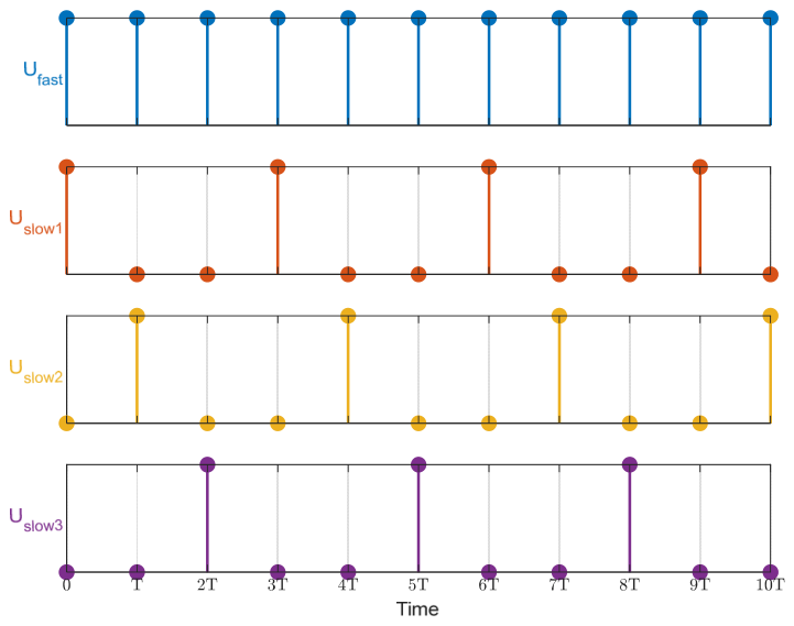
In the modal form, the controller is therefore decomposed into nine independent subsystems that must be allocated to different sampling periods. The first design step is to select the interlacing order $N$. For instance, for $N=3$, the controller must be split into four subspaces, denoted $R_{fast}$, $R_{slow1}$, $R_{slow2}$ and, $R_{slow3}$. 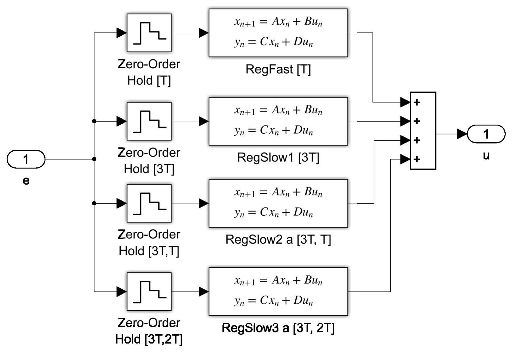The fast part is updated at every fast period $T$, whereas each slow part is updated every $N·T$ seconds, and their updates are phase-shifting such that, at each fast period $T$, the fast subsystem is evaluated together with exactly one slow subsystem. as illustrated in Figure 1 This results in a time-interlaced implementation of the overall control law.

Table 2. Separation of dynamics for $N=4$.

Mode	Poles
Fast	$0.1002,0.6648\pm 0.1448i$
Slow 1	$0.8009\pm 0.1105i$
Slow 2	$0.9031\pm 0.0356i,0.9057$
Slow 3	$0.9657,0.9723$
Slow 4	$0.9839\pm 0.0316i,1.0000$

illustrates a representative partition of the modal dynamics for an interlacing order $N=4$. The modes are grouped into one fast subsystem and four slow subsystems to obtain comparable orders across all fast periods (order 3 for the fast part and orders 2–3 for each slow part). This partition preserves all controller dynamics while effectively reducing the order that must be evaluated at each fast-sampling instant, thereby achieving a significant computational saving.

Since the controller comprises nine distinct dynamical modes, the maximum practical interlacing order with a fast part is $N=8$, obtained by assigning the fastest mode to the fast subsystem and each of the remaining eight modes to a different slow subsystem. In this case, the original 13th–order controller is implemented as a collection of interlaced controllers of order 2–3 evaluated at each fast-sampling instant, providing substantial computational savings while retaining all controller dynamics. A further alternative would be to consider $N=9$ without a dedicated fast part, assigning each mode to a subsystem operating at period $9T$ and updated consecutively, although this configuration generally entails a more pronounced degradation of closed–loop performance and is therefore of mainly theoretical interest.

4. Interlacing Controller

In this section, several strategies are presented to decompose the controller into interlaced components. Two main approaches are considered: a decomposition based on the diagonal (modal) form and another based on the balanced realization. In both cases, the objective is to separate the control action into one fast component and $N$ slow components, which can be expressed as follows:

$$u\left(k\right)=u_{Fast}\left(k\right)+\sum _{i=1}^N{u}_{Slowi}\left(k\right)$$

The fast part of the controller is updated with the fast-sampling period $T$, while the slow parts are updated with a slower period $N·T$; moreover, the latter are not updated simultaneously, but in a staggered fashion at consecutive fast sampling instants ($0, T, 2T, \dots , \left(N-1\right)T$).

The interlacing implementation admits several input–output sampling strategies, whose nomenclature follows the convention introduced in [9]. Regarding the input, strategy I-1 (Fast Input) feeds each slow block with the current fast-rate sample at the switching instant, whereas strategy I-2 (Slow Input) uses the same slow-rate sample for all slow blocks within the metaperiod. As for the output, strategy O-1 (Fast Change) holds the output of each slow block and updates it every time the block is activated, while strategy O-2 (Slow Change) accumulates the outputs of all slow blocks and injects their sum at the end of the metaperiod. In this work, two combinations are considered. In the first configuration (I1O2, fast input with slow output change), all slow controllers are evaluated at the same slow instant using the error available at that time, and their outputs are subsequently applied, one per fast period, in a phase-shifted fashion. In the second configuration (I2O2, slow input with slow output change), each slow controller is both computed and applied at the particular fast instant in which its output is used. From a computational standpoint, the I2O2 configuration is more efficient, since it reduces the amount of data that must be stored and propagated between sampling instants and provides control actions that are more up to date.

The decomposition is performed on the discrete-time controller with sampling period $T$, for both the diagonal and balanced representations. Once the controller has been partitioned, the slow parts are resampled to operate at period $N·T$. In multirate control systems, a similar change in sampling period to a meta-period $N·T$ is commonly used—known as lifting—to obtain an equivalent multirate representation [9,17,18,19]. In the interlacing scheme considered here, however, the period change is applied individually to each subsystem, and no global equivalent single-rate controller is required. In practice, this resampling operation can be implemented using standard discrete-time model conversion tools.

4.1. Diagonal Form

Starting from the controller discretized at period $T$ and expressed in diagonal modal form, the dynamics are separated into $N+1$ subsystems. One of these subsystems is assigned to the fast part, which remains at sampling period $T$, while the remaining $N$ subsystems constitute the slow parts, which are converted to operate at period $N·T$. In this representation, the controller can be written as:

$$G_{Reg}\left(z\right)=Re{g}_{fast}\left(z\right)+{\displaystyle \sum _{k=1}^N}Re{g}_{slow,k}\left(z\right)\approx Re{g}_{fast}\left(z\right)+{\displaystyle \sum _{k=1}^N}Re{g}_{slow,k}\left(z^N\right)·z^{-\left(k-1\right)}$$

This decomposition is closely related to the partial-fraction expansion of a SISO controller and extends naturally to the MIMO case in modal form. The allocation of each modal block to either the fast or one of the slow subsystems is performed using the ordering criteria discussed in Section 3 (e.g., pole magnitude, static gain, or Gramian-based measures), subject to the requirement of obtaining subsystems of comparable order and balanced dynamical content.

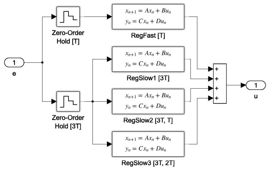
For a given interlacing order N, the overall structure of the I1O2 and I2O2 implementations in diagonal form follows the principles described in Section 3. The fast subsystem is evaluated at every fast-sampling instant $k·T$, whereas exactly one of the slow subsystems is evaluated and applied at each $k·T$ in a cyclic manner, as schematically depicted in Figure 2 (I1O2) and Figure 3 (I2O2). The diagonal realization offers two key advantages: the subsystems are dynamically decoupled from one another, and the original controller dynamics are exactly preserved within each block. This, in turn, leads to relatively simple implementation code and to predictable behavior when modifying the interlacing order or reassigning modes among the fast and slow parts.

4.2. Balanced Form

The balanced realization of a linear system is classically employed for model-order reduction, since it orders the states according to their joint controllability and observability, quantified by the Hankel singular values. Truncating the least significant states yields a reduced-order model at the expense of discarding part of the dynamics and slightly perturbing the remaining poles. In the present work, the balanced form is instead used to define an alternative interlacing decomposition that preserves all controller dynamics while distributing the balanced states among fast and slow subsystems.

In the balanced realization of the controller, the state vector is partitioned into one fast block and several slow blocks. For an interlacing order $N=3$, the controller can be written as:

$$\{\begin{array}{c} x_{Reg}\left(k+1\right)=\left[\begin{array}{c}{x}_{fast}\left(k+1\right)\\ x_{slow1}\left(k+1\right)\\ x_{slow2}\left(k+1\right)\\ x_{slow3}\left(k+1\right)\end{array}\right]=\left[\begin{array}{cccc}{A}_{11}& A_{12}& A_{13}& A_{14}\\ A_{21}& A_{22}& A_{23}& A_{24}\\ A_{31}& A_{32}& A_{33}& A_{34}\\ A_{41}& A_{42}& A_{43}& A_{44}\end{array}\right]·\left[\begin{array}{c}{x}_{fast}\left(k\right)\\ x_{slow1}\left(k\right)\\ x_{slow2}\left(k\right)\\ x_{slow3}\left(k\right)\end{array}\right]+\left[\begin{array}{c}{B}_1\\ B_2\\ B_3\\ B_4\end{array}\right]·u_{Reg}(k)\\ y_{Reg}\left(k\right)=\left[\begin{array}{cccc}{C}_{1 } & C_{2 }& C_{3 }& C_{4 }\end{array}\right]· x_{Reg}\left(k\right) +D_{Reg}·u_{Reg}\left(k\right)\end{array}$$

where the subscript “fast” denotes the block containing the most influential states according to the Hankel singular values, and “slow,i” denotes the blocks of decreasing importance.

Each block can be interpreted as a subsystem in which the remaining state components act as additional inputs. The fast subsystem is kept at the basic sampling period $T$, whereas the slow subsystems are converted to operate at the slower period $N·T$, and their outputs are applied at different fast sampling instants in an interlaced fashion, as schematically illustrated in Figure 1, according to either the I1O2 or I2O2 configuration. 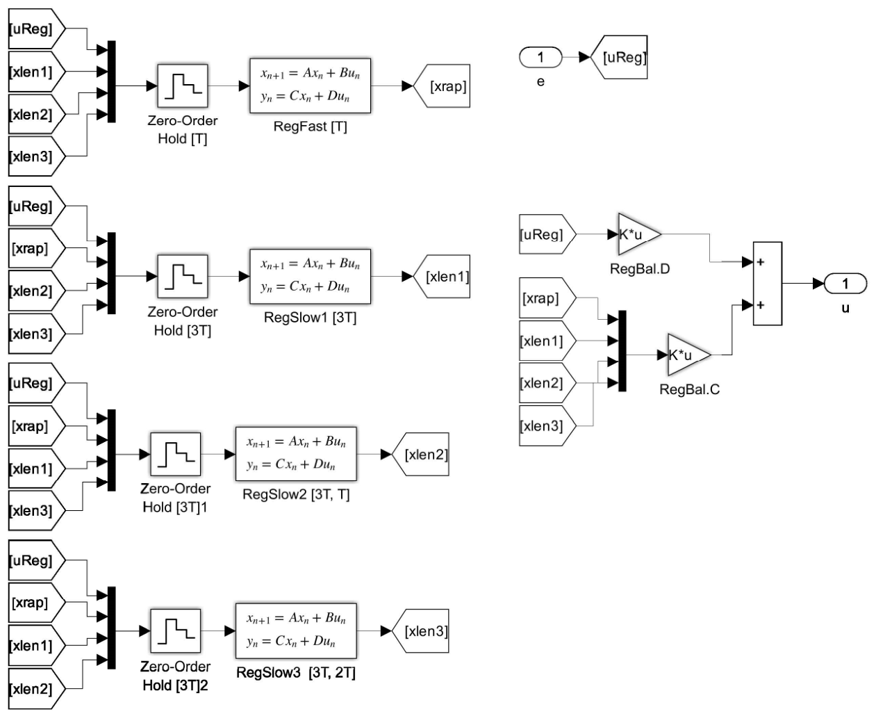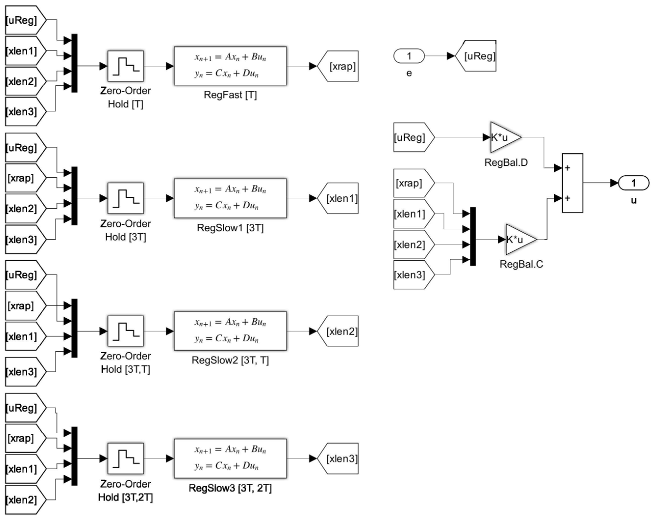In both cases, the output equation is evaluated at every fast period $T$, combining the contributions of the fast and slow parts to form the total control action. The resulting interlaced structures for the balanced-form controller are depicted in Figure 4 (I1O2) and Figure 5 (I2O2).

In the I1O2 configuration (Figure 4), all slow subspaces are evaluated using the controller input sampled at the same slow instant $N·T$, and their outputs are subsequently applied in a staggered manner over the next $N$ fast sampling instants, following the interlaced update pattern described above. In contrast, in the I2O2 configuration (Figure 5), each slow subspace is evaluated at the specific fast instant in which its output is applied, using the error available at that time. As in the diagonal case, the I2O2 implementation provides more up-to-date slow control actions and reduces memory requirements, but now this advantage must be weighed against the additional complexity induced by the state coupling among the balanced blocks.

To clarify the role of the coupling terms and the effect of the interlaced implementation, the balanced realization can be rewritten by explicitly isolating the fast and slow subspaces. This leads to the following state-space equations, where each subsystem is expressed in terms of its own states and the remaining state components are treated as additional inputs:

$$x_{fast}\left(k+1\right)=A_{11}·x_{fast}\left(k\right)+\left[\begin{array}{cccc}{B}_1& A_{12}& A_{13}& A_{14}\end{array}\right]·\left[\begin{array}{c}{u}_{Reg}\left(k\right)\\ x_{slow1}\left(k\right)\\ x_{slow2}\left(k\right)\\ x_{slow3}\left(k\right)\end{array}\right]$$

$$x_{slow1}\left(k+1\right)=A_{22}·x_{slow1}\left(k\right)+\left[\begin{array}{cccc}{B}_2& A_{21}& A_{23}& A_{24}\end{array}\right]·\left[\begin{array}{c}{u}_{Reg}\left(k\right)\\ x_{fast}\left(k\right)\\ x_{slow2}\left(k\right)\\ x_{slow3}\left(k\right)\end{array}\right]$$

$$x_{slow2}\left(k+1\right)=A_{33}·x_{slow2}\left(k\right)+\left[\begin{array}{cccc}{B}_3& A_{31}& A_{32}& A_{34}\end{array}\right]·\left[\begin{array}{c}{u}_{Reg}\left(k\right)\\ x_{fast}\left(k\right)\\ x_{slow1}\left(k\right)\\ x_{slow3}\left(k\right)\end{array}\right]$$

$$x_{slow3}\left(k+1\right)=A_{44}·x_{slow3}\left(k\right)+\left[\begin{array}{cccc}{B}_4& A_{41}& A_{42}& A_{43}\end{array}\right]·\left[\begin{array}{c}{u}_{Reg}\left(k\right)\\ x_{fast}\left(k\right)\\ x_{slow1}\left(k\right)\\ x_{slow2}\left(k\right)\end{array}\right]$$

The fast-state subspace ($x_{fast}$) is updated with period $T$ (at every instant $k$), whereas the slow states ($x_{slow,i}$) are resampled with period $N\cdot T$, with an offset such that the slow subspaces are updated sequentially over successive fast sampling periods $T$. Consequently, at instant $k$, only the fast subspace and one of the slow subspaces (denoted as $slow1$) are updated, while the remaining slow subspaces retain their values from the previous instant (zero-order hold). For example, for $N=3$, if at instant $k+1$ the slow1 subspace is updated, the others maintain their previous values:

$$x_{slow2}\left(k+1\right)=x_{slow2}\left(k\right)$$

$$x_{slow3}\left(k+1\right)=x_{slow3}\left(k\right)$$

At successive fast sampling instants, the remaining slow subspaces are updated, while the others retain their values from the previous instant.

The output equation is updated at the fast period $T$; however, the slow subspaces are updated at the slower period $N\cdot T$ in a staggered manner. Thus, at a given instant $k$, the output is updated together with the fast component and one of the slow components, while the other two slow components were updated at previous instants $k-1$ and $k-2$, respectively.

$$y_{Reg}\left(k\right)=C_1{x}_{fast}\left(k\right)+C_2{x}_{slow1}\left(k\right)+C_3{x}_{slow2}\left(k\right)+C_4{x}_{slow3}\left(k\right)+D_{Reg}{u}_{Reg}\left(k\right)$$

$$y_{Reg}\left(k\right)=C_1{x}_{fast}\left(k\right)+C_2{x}_{slow1}\left(k\right)+C_3{x}_{slow2}\left(k-2\right)+C_4{x}_{slow3}\left(k-1\right)+D_{Reg}{u}_{Reg}\left(k\right)$$

In this last equation, the effective instant at which each component in the output equation is updated is explicitly indicated.

A key difference with respect to the diagonal decomposition is that the dynamics of the separated balanced subspaces do not coincide exactly with the original modal dynamics. The off-diagonal coupling terms $A_{ij}$ give rise to a residualisation effect: the poles associated with each separated subsystem are shifted with respect to their locations in the original controller, and this effect is particularly pronounced in the least significant states.

From an implementation viewpoint, the balanced-form interlacing structure is more involved than the diagonal one, since all subsystems are dynamically coupled, and their states must be stored and updated consistently across sampling instants. This leads to a higher coding effort and increases computational cost, partially offsetting the savings obtained by interlacing. Nevertheless, the balanced-form approach provides a systematic way of assigning the most influential states—according to Hankel singular values—to the fast subsystem, which may be advantageous in applications where state importance is a more suitable design criterion than pole location. In the case study considered, however, the numerical results reported later in the paper indicate that diagonal-form interlacing offers a better trade-off between performance and implementation complexity than the balanced-form counterpart, especially for higher interlacing orders.

In fact, the interlacing decomposition described above can be applied to any state-space realization of the controller and is not restricted to the balanced form. One may work with an arbitrary state-space representation and decide which states are assigned to each part of the controller according to the design objectives. The balanced realization provides a systematic way of ordering the states based on their controllability–observability Gramians, but alternative partitioning criteria could equally be adopted when other performance or implementation aspects are to be prioritized.

5. Results

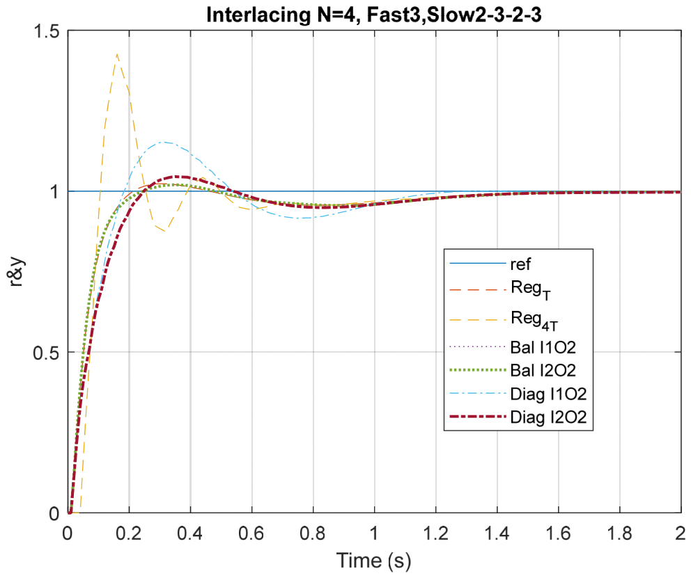
An interlaced implementation with interlacing order $N=4$ has been evaluated in four different configurations, combining the two controller decompositions (diagonal and balanced) with the I1O2 and I2O2 update schemes. Under a unit-step reference in yaw rate, the corresponding closed-loop responses are displayed in Figure 6. All interlaced configurations exhibit a behavior that lies between that of the full controller operating at the fast-sampling period $T$ and that of the same controller operating at the slow period $4T$, thereby confirming that interlacing provides an intermediate trade-off between computational saving and dynamic performance. Among the four cases, the diagonal I1O2 configuration yields the most degraded response, which is consistent with the fact that all slow control actions are computed at the same slow instant and subsequently applied with delay.

These results demonstrate that the interlacing strategy can reduce the computational effort required at each fast-sampling instant without explicitly discarding any of the dynamics of the original controller. In particular, the I2O2 configurations, both for the diagonal and the balanced realizations, provide responses that are significantly closer to that of the complete controller at period $T$. This improvement can be attributed to the use, in each slow subsystem, of the error signal measured at the same instant at which its control action is applied, which yields more up-to-date control inputs and partially compensates for the increased effective sampling period of the slow parts.

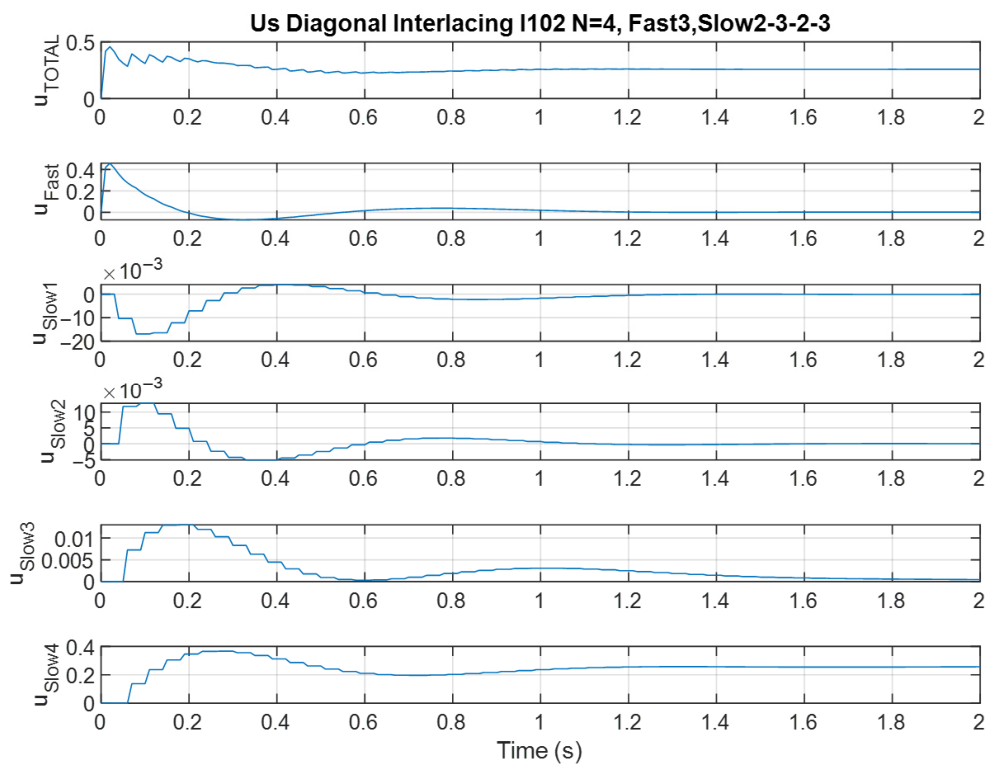
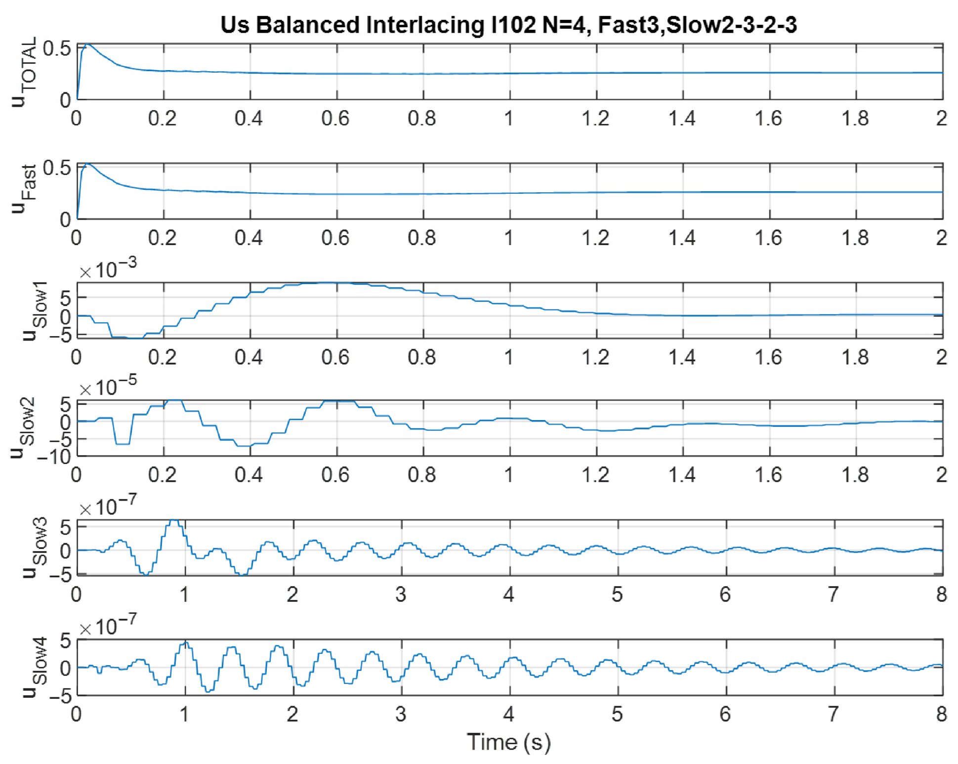
Further insight into the differences between the diagonal and balanced decompositions can be obtained by analyzing the individual contributions of the fast and slow components to the total control action. Figure 7 shows the control signals generated by the balanced-form interlaced controller, whereas Figure 8 depicts the corresponding signals for the diagonal-form interlaced controller. In the balanced case (Figure 7), the most delayed slow components exhibit very limited influence on the total control action, and a small-amplitude oscillation with slow attenuation can be observed in the slowest parts, which is not desirable from a control standpoint. By contrast, in the diagonal case (Figure 8) the contributions of the different subsystems are more evenly distributed, and no such oscillations appear, indicating that the diagonal decomposition achieves a more homogeneous sharing of the control effort while preserving the original controller dynamics.

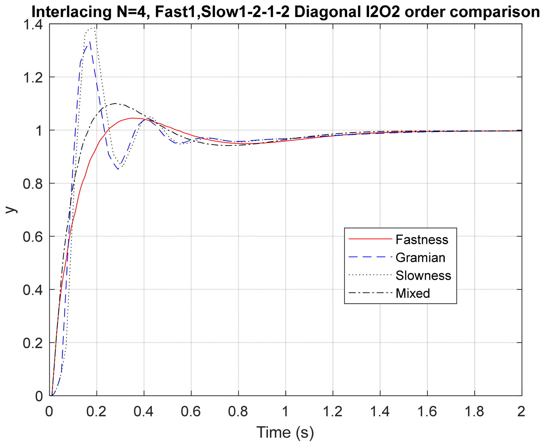
The effect of the ordering of the interlaced subsystems in the diagonal I2O2 configuration has also been investigated. Figure 9 compares several ordering criteria, including sorting the modes by speed (from the fastest to the slowest poles), by Gramian-based importance, and a mixed criterion based on the amplitude of the individual control actions. The ordering based on speed provides the best compromise between settling time and overshoot. The mixed criterion leads to a slightly faster response but at the expense of a higher overshoot, whereas the orderings based on inverse speed or solely on Gramian values yield behaviors more similar to that obtained with the controller operating at the slow sampling period and are therefore less favorable from a performance perspective.

To select an appropriate interlacing order $N$, it is convenient to define a cost index that jointly weights the degradation in control performance induced by increasing $N$ and the corresponding computational savings, with the aim of determining an optimal solution that reduces the computational burden without excessively compromising the closed-loop performance. The specific choice of this index largely depends on the application in which the interlacing strategy is implemented, and in some cases an excessively high value of $N$ may even lead to a complete loss of control. 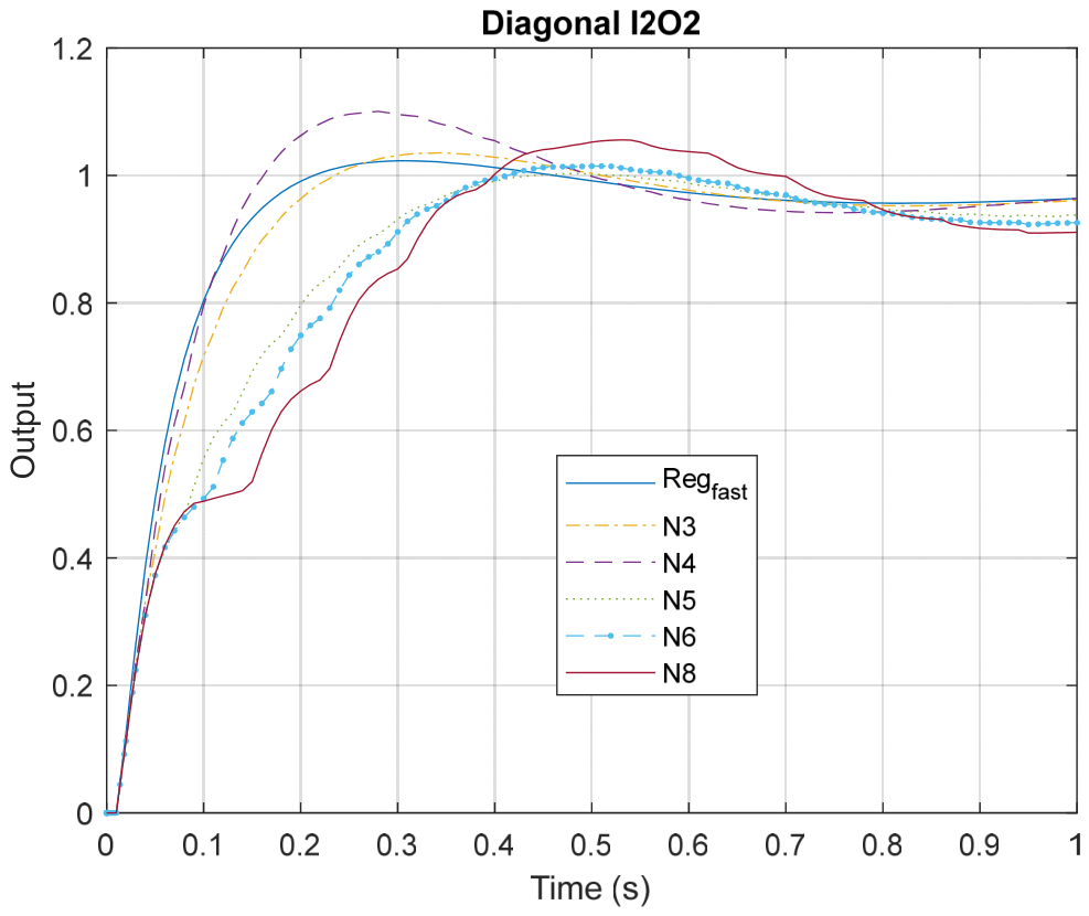Figure 10 provides a detailed illustration of the deterioration of the closed-loop behavior as $N$ increases for a diagonal interlacing I2O2 controller applied to yaw-rate control.

Finally, the impact of increasing the interlacing order has been assessed by implementing a diagonal-form interlaced controller with $N=8$. The corresponding closed-loop responses are presented in Figure 10. As expected, the larger value of $N$ results in a more pronounced degradation of the transient performance, with increased overshoot and slower convergence, despite the additional computational savings associated with the further reduction in the effective order evaluated at each fast-sampling instant. This observation confirms the existence of a trade-off between computational load and control performance and suggests that very high interlacing orders should only be employed when the resulting deterioration remains acceptable for the specific application.

6. Computational Savings

The computational load of a controller over a sampling period $T$ can be approximately estimated from the number of arithmetic operations (multiplications and additions) required by its state equations. In this analysis, the computational cost associated with evaluating the controller output equation is not considered, as it is identical for all configurations under study. For a controller with $n$ states and $p$ inputs, in which all state variables influence each other—as in the balanced realization—the computational cost can be expressed as:

$$C_{op}=n·\left(n+p\right)$$

If the structure of the state equations is simpler, this cost can be significantly reduced. The simplest case corresponds to the diagonal structure, in which each state variable depends only on itself. In this case, a similar computational simplification is performed for robust controllers in active magnetic bearing systems by Sahinkaya and Sawicki in [20]. Thus, for the diagonal state-space structure, the computational cost reduces to:

$${Cd}_{op}=n·\left(1+p\right)$$

Therefore, the use of a diagonal implementation already implies a computational saving, which can be estimated as:

$$Sd=\left(1-{\displaystyle \frac{C{d}_{op}}{C_{op}}}\right)=1-{\displaystyle \frac{1+p}{n+p}}={\displaystyle \frac{n-1}{n+p}}$$

In an interlacing implementation of order $N$, the states are distributed between a fast subcontroller of order $n_f$ and $N$ slower subcontrollers (with average order given by $n_s=\left(n-n_f\right)/N$). In this scheme, at each fast-sampling period only the fast subcontroller and one of the slow subcontrollers are evaluated. As the interlacing order $N$ increases and the order of the fast subcontroller $n_f$ decreases, the computational savings increase. However, this reduction is achieved at the expense of a potential degradation in performance with respect to the non-interlaced controller. The resulting computational cost, for both the balanced and diagonal forms, can be estimated as:

$$C_N=\left(n_f+n_s\right)·(n+p)$$

$${Cd}_N=\left(n_f+n_s\right)·(1+p)$$

The computational savings obtained by applying interlacing, for both structures, can be calculated as:

$$S_N=\left(1-{\displaystyle \frac{C_N}{C_{op}}}\right)=\left(1-{\displaystyle \frac{{Cd}_N}{{Cd}_{op}}}\right)={\displaystyle \frac{n-(n_f+n_s)}{n}}$$

For the considered application, with $n=1$ states and $p=1$ inputs, the computational saving achieved by using the diagonal realization instead of the balanced one is $Sd=87.5\%$. If an interlacing scheme with $N=4$ and a fast subcontroller of order $n_f=7$ is applied to the controller under study, the computational saving due to interlacing is $S_N=40\%$.

Finally, regarding the differences in computational load between the I1O2 and I2O2 configurations, it should be noted that in the I2O2 configuration the computational load is uniformly distributed across all sampling periods. In contrast, in the I1O2 configuration the load is not evenly distributed: all slow control actions are computed within a single period and subsequently applied with a time shift. As a result, the computational load is concentrated in the first fast period $T$ of each metaperiod $N·T$, where no computational savings are achieved, whereas in the subsequent periods a significant reduction is observed.

7. Conclusions

This work has examined the implementation of a high-order robust controller for lateral guidance of an autonomous vehicle by means of an interlacing strategy. The resulting closed-loop behavior has been shown to lie between that of the original controller operating at the fast sampling period ($T$) and that of the same controller operating at a slower period ($N T$), thereby providing an intermediate compromise between computational saving and dynamic performance. In practice, the interlaced realization behaves as an effective lower-order controller evaluated at the fast period while preserving all the dynamics of the original design.

The appropriate choice of the interlacing order $N$, which fixes the slow period as an integer multiple of the fast period, requires a dedicated analysis of the controller dynamics. As $N$ increases, the performance degradation associated with the slower update of the slow subsystems becomes more pronounced, and it is therefore necessary to verify that the resulting closed-loop response remains acceptable for the application at hand. Once $N$ has been selected, the controller modes should be distributed between the fast subsystem and the $N$ slow subsystems so that their orders are as similar as possible, thereby achieving a balanced effective order at each fast-sampling instant.

Regarding the structural configurations, the update schemes in which the slow control actions are computed using the error measured at the same instant at which they are applied (I2O2) have been observed to provide better results than those in which all slow actions are computed at the same slow instant and subsequently applied with delay (I1O2). By yielding more up-to-date control inputs and reducing the amount of information that must be stored between sampling instants, these implementations offer both improved closed-loop behavior and a more efficient use of computational resources. A comparison between the diagonal and balanced realizations has revealed that the best closed-loop behaviors are consistently obtained with the diagonal interlacing, particularly for larger values of the interlacing order ($N$), while also leading to simpler implementation structures.

Although interlaced controllers have already been considered in previous applications, mainly in transfer-function form for SISO systems, the main contribution of the present work lies in formulating the interlacing decomposition directly on a state-space representation of a given robust controller and extending it to MIMO systems of arbitrary dimension. In this sense, the emphasis is placed on a practical implementation and decomposition strategy that clarifies the trade-off between computational load and closed-loop behavior for high-order controllers in an automotive context, rather than on proposing a new multirate control theory. The simulation results obtained under conditions representative of a test-track circuit indicate that substantial reductions in computational effort can be achieved at the expense of a moderate deterioration of the closed-loop response, suggesting that the proposed approach may constitute a useful tool for the real-time implementation of complex robust controllers on embedded platforms.