


Abstract
To address the challenges of constrained grid-like compartments, a motion framework integrating adaptive obstacle avoidance planning and active disturbance rejection control is proposed. First, an Adaptive Rapidly exploring Random Tree Star (Adaptive RRT*) algorithm based on multi-source state feedback is developed. Scaled-down model simulations show that, compared to conventional algorithms, its path length (374.28 mm), planning time (0.30 s), and node count (50.83) are reduced by at least 29.5%, 64.7%, and 28.6%, respectively, achieving a 100% planning success rate. Next, a control scheme based on Extended State Observer–Model Predictive Control (ESO-MPC) is designed. Simulations indicate that under nominal conditions, tracking errors are reduced by 5.78–84.35% compared to traditional MPC. Under a 20% link mass perturbation, the scheme effectively eliminates phase lag. Under complex scenarios involving parameter perturbation and a 0.6 N·m step torque disturbance, the tracking error reduction ranges from 25.27% to 87.59%, exhibiting excellent disturbance rejection robustness. Physical experiments conducted on a scaled-down experimental platform further verify that the maximum tracking errors of the manipulator end-effector along the x, y, and z axes under ESO-MPC are 0.88 mm, 0.85 mm, and 0.89 mm, respectively, significantly outperforming the 2.41 mm, 2.39 mm, and 2.47 mm observed with MPC. Finally, obstacle avoidance and trajectory-tracking simulations of an industrial manipulator in a full-scale ship compartment environment validate the engineering feasibility of the proposed framework.
1. Introduction
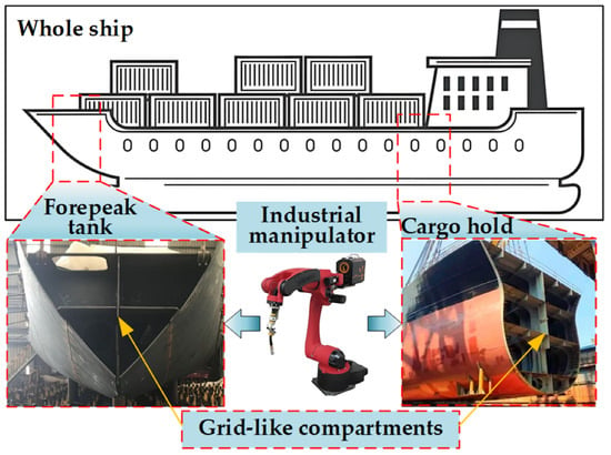
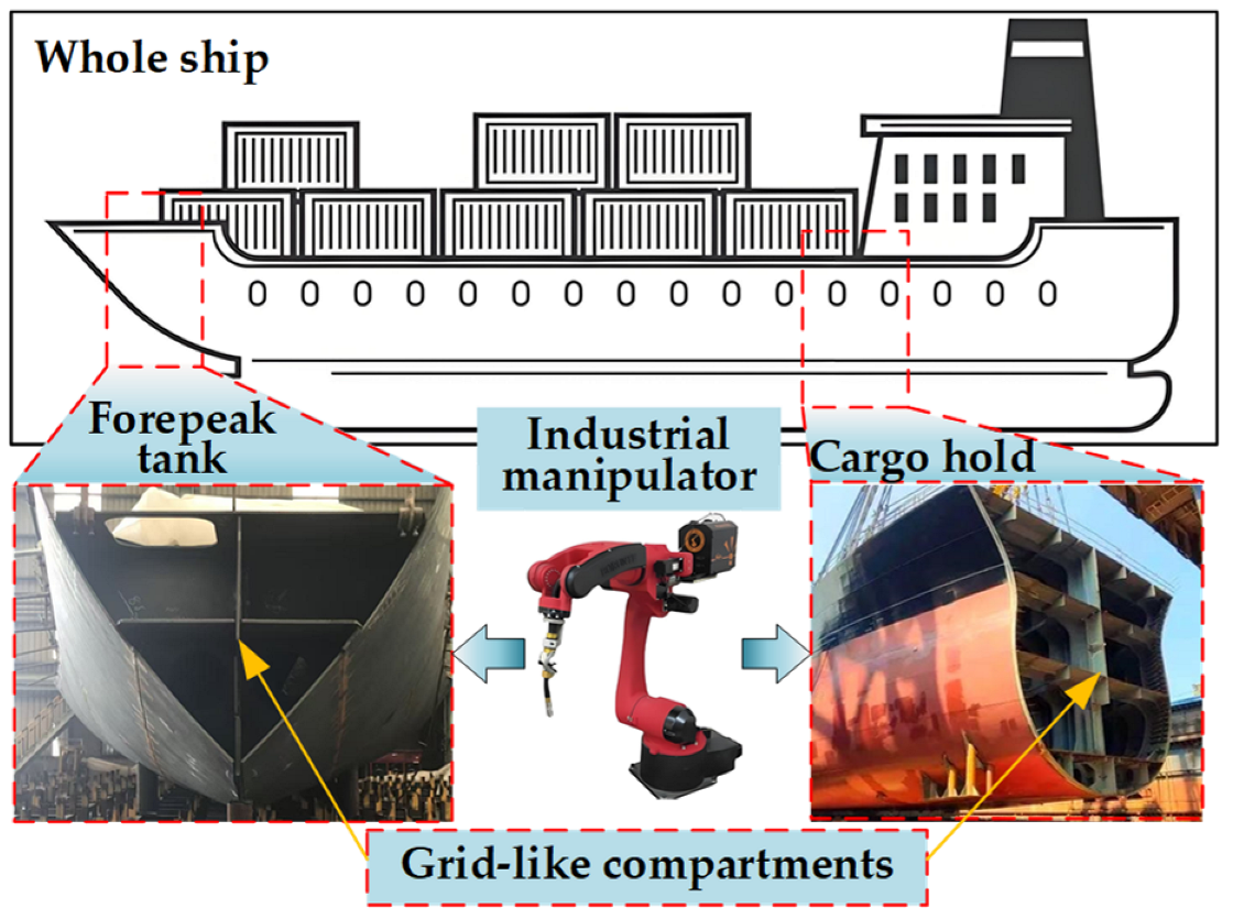
In modern shipbuilding, grid-like compartments are essential hull components, as shown in Figure 1. Due to the dense arrangement of beams and ribs, these compartments form highly constrained and complex narrow spaces [1,2]. Traditional mechanized or manual operations in such environments often face significant challenges regarding operational efficiency and flexibility [3,4]. Industrial manipulators have thus emerged as a vital automation solution for these structures. To ensure the reliable execution of tasks in such environments, efficient collision-free path planning and high-precision trajectory-tracking control remain two fundamental technical challenges [5,6].
Figure 1.
Grid-like structures in a ship.
In the field of robotic path planning, the Artificial Potential Field (APF) method, Swarm Intelligence Optimization (SIO) algorithms, Rapidly exploring Random Tree (RRT) algorithms, and learning-based algorithms have been extensively investigated. Although these classical algorithms perform well in conventional scenarios, they face severe challenges when dealing with complex high-dimensional or highly constrained environments. Specifically, while APF possesses excellent real-time performance, it is highly susceptible to local optima in dense obstacle environments and often suffers from oscillations and reachability issues near the target due to the balance between attractive and repulsive forces [7]. SIO algorithms (such as Particle Swarm Optimization, PSO, and Whale Optimization Algorithm, WOA), though capable of heuristic optimization of path length, exhibit low convergence efficiency in complex constrained spaces. Furthermore, these algorithms are highly sensitive to initial parameters, making it difficult to balance real-time obstacle avoidance with global search capabilities [8]. Learning-based algorithms (such as Deep Deterministic Policy Gradient, DDPG; Twin Delayed Deep Deterministic Policy Gradient, TD3; and Iterative Learning Control, ILC) rely heavily on large-scale offline pre-training of samples, which involves significant computational overhead. Moreover, they exhibit insufficient generalization capabilities when facing random perturbations in unstructured environments, making it difficult to guarantee control robustness under complex operating conditions [9,10,11]. In contrast, RRT algorithms possess probabilistic completeness through random sampling and tree expansion mechanisms, allowing for the rapid exploration of high-dimensional spaces without the need for complex environmental pre-processing. Although such algorithms demonstrate significant potential in handling complex constraints, their original forms still possess inherent limitations, such as a lack of asymptotic optimality, high path redundancy, and unstable convergence speeds [12,13].
To address these issues, researchers have implemented profound improvements to RRT and its variants in recent years. Regarding sampling strategies and search efficiency, Liang et al. [14] proposed the AGP-RRT* algorithm, utilizing adaptive biased sampling and adjustable step-sizes to accelerate search speeds. Zhao et al. [15] introduced the GD-RRT* algorithm based on Gaussian mixture probability distributions; by alternating between Gaussian and target-biased sampling, the planning efficiency of initial paths was substantially improved. Furthermore, Ku et al. [16] integrated dynamic elliptical sampling and APF-guided strategies to enhance exploration in complex spaces through local rewiring. In terms of path quality and adaptability, Jeong et al. [17] introduced the Quick-RRT* algorithm to reduce costs and improve smoothness by expanding the parent vertex set. Qi et al. [18] proposed a multi-objective dynamic RRT* algorithm that ensures high-quality initial paths through refined replanning. Additionally, Qi et al. [19] developed a two-stage optimized RRT using heuristic sampling, which reduced invalid exploration by 62.9% for Six-Degrees-of-Freedom (6-DOF) manipulators. Moreover, Xiong et al. [20] improved tree expansion through a node classification framework to enhance convergence, while Guo et al. [21] utilized adaptive directional bias and path pruning to reduce planning time. Meanwhile, Cheng et al. [22] employed multi-tree parallel expansions to address slow expansion in large-scale spaces.
However, most existing studies focus on open or sparsely obstructed environments, failing to account for the extremely confined spaces and irregular geometric constraints of grid-like structures. Consequently, current algorithms often exhibit excessive randomness and low efficiency in such environments, making it difficult to generate paths that meet the requirements for stable manipulator operations. Therefore, it is of great engineering value to develop an improved planning algorithm for ship grid-like compartments that balances reliability with path quality.
Robotic manipulators, as multivariable coupled systems, face precision challenges from parameter perturbations and external disturbances [6,23,24]. Conventional methods like Proportional–Integral–Derivative (PID), adaptive, and sliding-mode control [25,26,27] often struggle under significant disturbances due to their heavy reliance on accurate dynamic models. To address this, the Extended State Observer (ESO) treats uncertainties as a “lumped disturbance” for real-time compensation, simplifying complex dynamics into nominal models and reducing dependency on high-order parameters.
Building upon these nominal models, Model Predictive Control (MPC) has emerged as a cornerstone for multivariable tracking due to its superior constraint-handling and optimization capabilities [28,29,30]. In terms of theoretical frameworks and foundational algorithms, Dai et al. [31] proposed a tube-based MPC that ensures robust stability in complex environments by tightening nominal system constraints. Chen et al. [32] introduced Quantum Particle Swarm Optimization (QPSO) to enhance MPC solving efficiency and tracking precision for complex tasks, while Li et al. [33] developed a hierarchical multi-loop MPC scheme integrated with feedback linearization and Nonlinear Disturbance Observers (NDOs) to improve robustness. In recent years, MPC has achieved breakthroughs in both theory and application. Regarding robust disturbance rejection, Yang et al. [34] proposed an event-triggered MPC framework combined with disturbance observers to simplify optimization while guaranteeing stability. Deng et al. [35] developed a unified predictive architecture using Lyapunov-based constraints to reduce computational overhead. Concerning intelligent integration, Hong et al. [36] combined Deep Reinforcement Learning (DRL) with MPC to overcome traditional obstacle avoidance limitations, while Wang et al. [37] and Li et al. [38] achieved synergy between path generation and tracking control by improving the Dynamic Window Approach (DWA) or A* algorithms.
However, the extremely confined space within ship grid-like compartments necessitates frequent and sharp maneuvers of the manipulator. This imposes stringent requirements on the controller’s transient response and introduces high-frequency, stochastic dynamic disturbances. Existing standalone MPC or observer-based schemes often struggle to balance high tracking precision with real-time computational efficiency.
To this end, this study proposes an ESO-MPC composite control framework. The framework utilizes the ESO to estimate and compensate for lumped internal and external disturbances in real-time, thereby simplifying complex dynamics into a nominal state-space model to provide accurate state estimation for MPC receding-horizon optimization. Based on this, the MPC handles actuator constraints to achieve precise trajectory tracking. This integrated paradigm of active disturbance rejection and predictive optimization significantly enhances the system’s adaptability to complex, constrained environments and ensures smooth operation with minimal computational latency.
The overall research methodology follows a “planning–control–verification” framework, aiming to address the challenges of obstacle avoidance planning and high-precision tracking for a 6-DOF manipulator in constrained ship compartment environments. At the planning level, an Adaptive RRT* algorithm based on multi-source state feedback is proposed. Through comparative simulations with mainstream RRT series algorithms in scaled-down ship compartments, the performance of the proposed algorithm in enhancing search efficiency and path quality is quantitatively evaluated using path length, computation time, node count, and success rate as metrics. At the control level, an ESO-MPC composite controller is designed. Through three types of simulations, including nominal, parameter perturbation, and external-disturbance scenarios, its performance gain in enhancing tracking accuracy and disturbance rejection robustness is systematically evaluated. On this basis, a scaled-down experimental platform is utilized to verify the actual performance of the control algorithm via the spatial position error of the end-effector. Finally, the engineering feasibility of the framework is confirmed through obstacle avoidance and trajectory-tracking simulations of an industrial manipulator in a full-scale ship compartment environment.
The remainder of this paper is organized as follows: Section 2 establishes and validates the kinematic model of the 6-DOF manipulator. Section 3 presents the Adaptive RRT* algorithm and quintic B-spline interpolation for obstacle avoidance planning. Section 4 designs the ESO-MPC composite controller and conducts both simulation and experimental verification. Finally, the conclusion is given in Section 5.
2. Kinematic Modeling and Verification of the 6-DOF Manipulator
In this section, the forward-kinematics (FK) and inverse-kinematics (IK) models of a customized 6-DOF manipulator are established and verified. The manipulator is a physical prototype developed by scaling down the classic PUMA 560 industrial manipulator at a 1:5 ratio. Utilizing this scaled-down prototype enables safe, cost-effective, and rigorous experimental validation of control strategies prior to their deployment on full-scale industrial equipment. The core technical parameters of the manipulator are detailed in Table 1.
Table 1.
Technical parameters of the 6-DOF manipulator.
2.1. FK Modeling
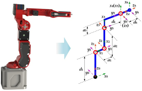
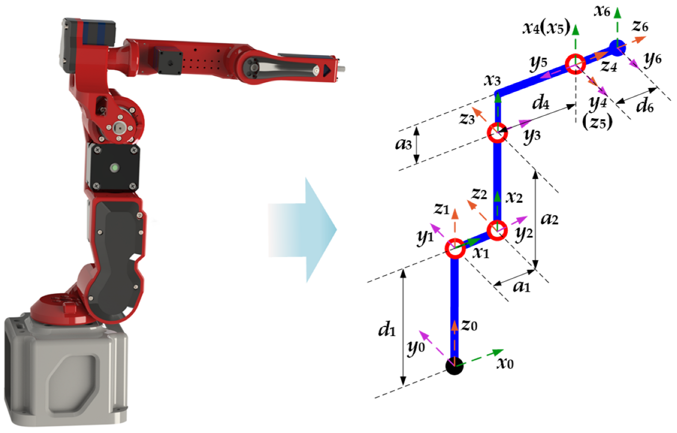
The 3D model of the 6-DOF manipulator and its link coordinate frames established based on the D-H method are shown in Figure 2, and the corresponding D-H parameters are detailed in Table 2.
Figure 2.
3D model and D-H coordinate frames of the 6-DOF manipulator.
Table 2.
D-H parameters of the 6-DOF manipulator.
In Table 2, i denotes the link index, αi−1 is the link twist, ai−1 is the link length, di is the link offset, and θi is the joint angle.
Based on the D-H parameters, the homogeneous transformation matrix between adjacent links can be obtained using the standard transformation formula. Consequently, the forward-kinematics equation of the manipulator, representing the pose of the end-effector relative to the base, can be expressed as a cascade of transformation matrices:
where R3×3 and P3×1 represent the orientation rotation matrix and spatial position vector of the end-effector in the base coordinate frame, respectively.
2.2. IK Modeling
Since the axes of the last three joints (Joints 4, 5, and 6) intersect at a single point (the wrist center), the manipulator satisfies Pieper’s criterion, ensuring the existence of closed-form analytical solutions for the inverse kinematics. The IK calculation is decoupled into two independent processes: position solving and orientation solving. First, the spatial coordinates of the wrist center are extracted from the end-effector pose matrix, and the first three joint angles θ1, θ2, and θ3 are obtained using algebraic and simplified geometric methods. Subsequently, using the calculated first three joint angles and the overall orientation matrix, the wrist joint angles θ4, θ5, and θ6 are analytically derived.
Because multiple analytical solutions exist for IK, a weighted joint delta is introduced to ensure the continuity and smoothness of the manipulator’s motion during trajectory tracking. During the calculation, the solution that minimizes is consistently selected as the optimal inverse solution:
where Δθi is the angle variation of the i-th joint from the previous path point to the current one; ki is the weight factor, set as k1 = k2 = k3 = 1.0, and k4 = k5 = k6 = 0.5.
2.3. Simulation Verification
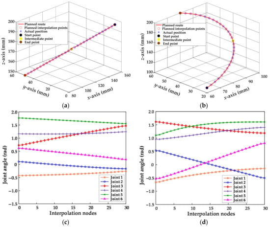
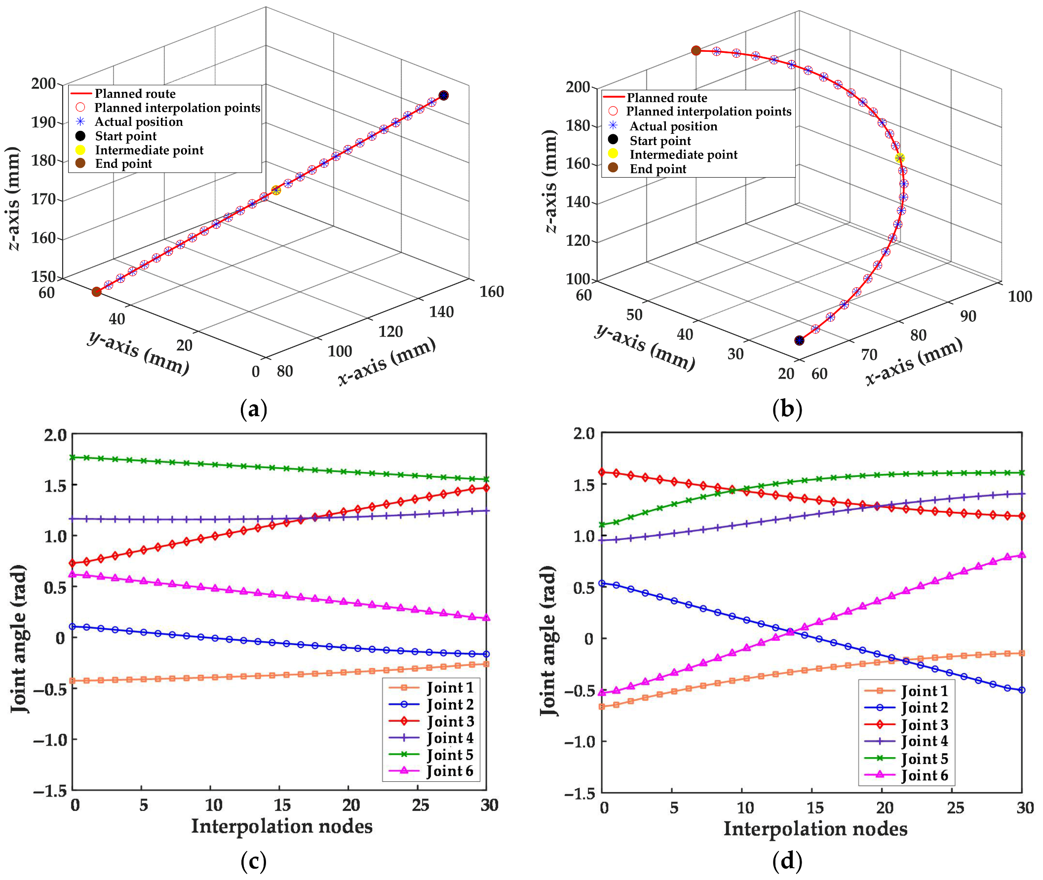
A simulation model of the manipulator is constructed using the Robotics Toolbox in MATLAB 2023a. To verify the accuracy of the kinematic models, linear- and circular-trajectory-tracking simulations are conducted with the end-effector origin as the target. The linear path is planned from [150, 0, 200] to [80, 50, 150], and the circular path passes through the start point [60, 20, 110], mid-point [100, 40, 150], and end point [80, 60, 200]. The IK is solved for the discrete path points to obtain the optimal joint angles, which are then substituted into the FK model to calculate the actual poses. The results are shown in Figure 3.
Figure 3.
Path tracking results and joint angle trajectories: (a) Linear-path tracking; (b) circular-path tracking; (c) joint angle curves for linear motion; (d) joint angle curves for circular motion.
As seen in Figure 3a,b, the actual terminal trajectories perfectly coincide with the theoretically planned paths. Figure 3c,d demonstrate that the joint angle trajectories are smooth, continuous, and free of abrupt changes. The simulation results fully verify the accuracy of the kinematic models and the effectiveness of the optimal inverse solution selection strategy.
3. Obstacle Avoidance Trajectory Planning in Constrained Environments
To address the issue that the traditional RRT* algorithm is prone to falling into local minima and exhibits rigid search behaviors in confined spaces with complex constraints, the Adaptive RRT* is proposed in this section. This algorithm introduces a multi-source state feedback mechanism to dynamically calculate the adaptive goal bias probability Pt and the adaptive greedy extension probability Pm to generate discrete paths. Subsequently, a quintic B-spline interpolation is employed to convert the discrete paths into smooth and continuous trajectories, effectively enhancing the trajectory quality.
3.1. Adaptive RRT* Algorithm for Path Planning
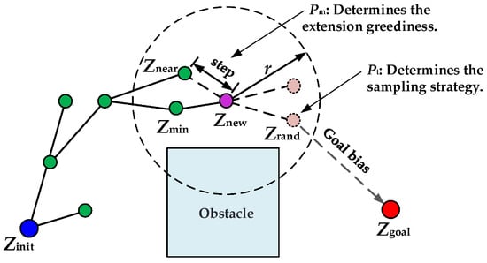
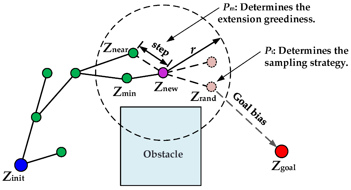
Although the RRT* algorithm performs well in path optimization, fixed parameters often lead to rigid algorithm behaviors when the manipulator operates in confined spaces, faces joint limit constraints, or encounters complex curved obstacles, making it highly susceptible to local minima. To address this limitation, an adaptive parameter adjustment mechanism based on multi-source state feedback (composed of distance convergence and search stagnation) is proposed. This mechanism dynamically calculates Pt and Pm by extracting the growth characteristics of the search tree in real-time. In conventional open areas, this strategy maintains a strong goal bias and a large extension step size to ensure convergence speed; when search stagnation is detected, it dynamically adjusts the probability thresholds to force the algorithm into a large-scale global random search, significantly enhancing the capability to escape local optima. The principle of the Adaptive RRT* algorithm is shown in Figure 4.
Figure 4.
Schematic diagram of the Adaptive RRT* algorithm.
Two key state feedback factors are introduced into the algorithm: the distance convergence degree Rdist and the search stagnation penalty factor Cpenalty. Rdist is used to evaluate the macroscopic progress of the search tree approaching the target, defined as the ratio of the shortest distance to the target in the tree dmin to the initial distance dmax:
As the search progresses, Rdist gradually converges from 1 toward 0. Cpenalty characterizes the complexity of the local space and the degree to which the algorithm is trapped in local minima. If the newly generated node fails to expand multiple times consecutively due to collisions or IK unreachability, the penalty is increased by the continuous failure count Nfail. Cpenalty is directly proportional to Nfail:
where K is the failure tolerance constant (set to K = 25), and Cmax is the maximum penalty limit (set to Cmax = 0.6) to prevent the algorithm from degenerating into a purely blind random search due to excessive penalization.
Pt determines the probability of directly selecting the target point as the sampling point during heuristic sampling. The update rule is formulated as follows:
where the base probability Pt,base is 0.15, and the truncation interval is [0.05, 0.5]. When an increase in Nfail triggers the penalty, Pt decreases rapidly, forcing the algorithm to abandon the local greedy strategy and switch to random sampling in a broader space to escape the local trap.
Pm determines whether the algorithm adopts a conservative fixed single step size or a more aggressive large step size when growing toward the sampling point. The update rule is formulated as follows:
where Pm,base is 0.2, Wdist is the distance weight factor (set to 0.6), and the truncation interval is [0.05, 0.9]. As the search tree approaches the target (Rdist decreases), Pm gradually increases, promoting the rapid closure of the path with large step sizes under collision-free conditions; once a collision occurs, Cpenalty immediately suppresses this aggressive behavior and restores fine exploration with small step sizes.
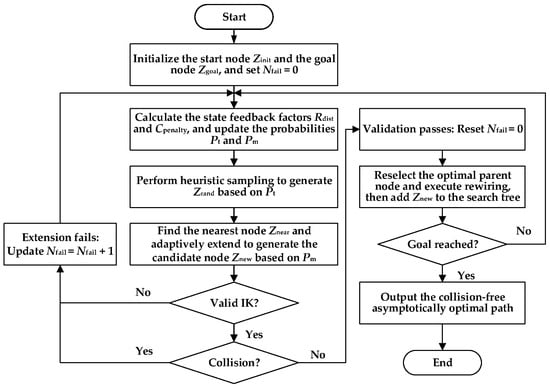
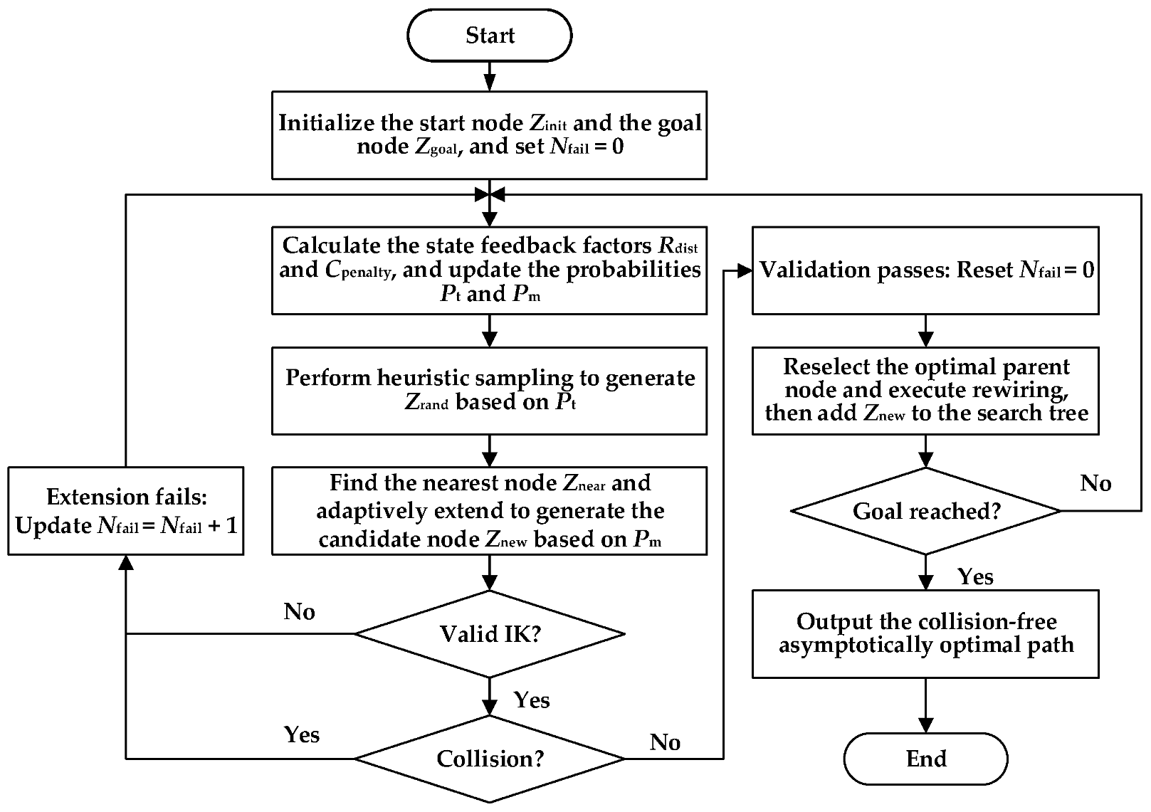
The Adaptive RRT* algorithm is utilized for the obstacle avoidance path planning of the manipulator. The flowchart is shown in Figure 5, and the specific steps are as follows:
Figure 5.
Flowchart of the Adaptive RRT* algorithm for path planning in confined environments.
Step 1: Input the working environment, start position Zinit, and goal position Zgoal. Initialize Nfail = 0, and calculate dmax.
Step 2: Multi-source feedback calculation. Extract dmin from the tree to calculate Rdist. Calculate Cpenalty based on Nfail, and update Pt and Pm in real-time.
Step 3: Heuristic sampling. Generate a random number . If Prand1 < Pt, the sampling point is set as Zrand = Zgoal; otherwise, randomly sample in the state space to obtain Zrand.
Step 4: Nearest-neighbor search and adaptive growth. Find the nearest node Znear to Zrand in the tree. Generate a random number . If Prand2 < Pm, perform a large-step greedy extension toward Zrand to generate a tentative node Znew; otherwise, generate Znew with a fixed short step size.
Step 5: IK constraint verification. Solve the IK for Znew. If no solution exists, discard the node, increment Nfail = Nfail + 1, and return to Step 2.
Step 6: Collision detection constraint verification. Perform collision detection on the local path connecting Znear and Znew. If a collision occurs, discard the node, increment Nfail, and return to Step 2; if no collision occurs, the local path is physically feasible, retain Znew, and clear Nfail to 0.
Step 7: Asymptotically optimal topological reconstruction. Define a neighborhood of radius r around Znew. Using cumulative spatial distance as the path cost, connect Znew to the neighbor providing the minimum-cost, collision-free path. Subsequently, rewire the neighborhood to optimize topological connections under the same collision-free constraint.
Step 8: Loop the above steps until the goal point is connected, and finally output the collision-free, asymptotically optimal path of the manipulator.
3.2. Simulation and Analysis of Trajectory Planning
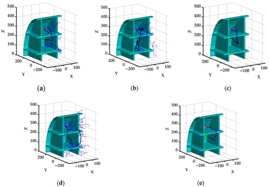
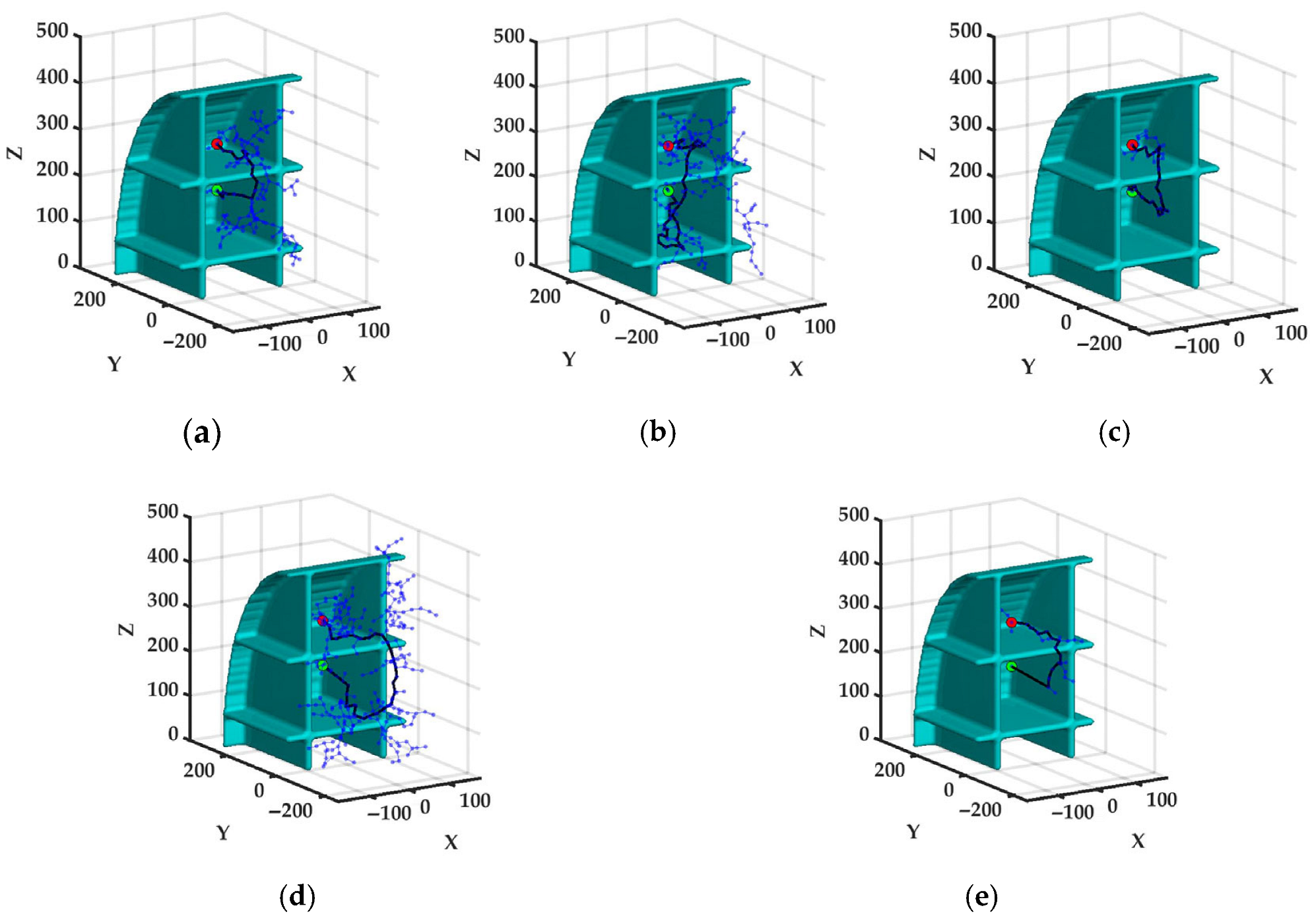
Using a 1:5 scaled ship compartment model, obstacle avoidance path planning for crossing a longitudinal web frame is simulated in MATLAB. The search space is defined as 400 × 500 × 500 mm, with start and goal coordinates at (0, 100, 300) mm and (0, 100, 200) mm, respectively. Five algorithms, including RRT, RRT*, RRT-Connect, Informed RRT*, and Adaptive RRT*, are evaluated over 100 independent trials with a 10,000-iteration limit. Figure 6 compares the resulting paths from a single simulation.
Figure 6.
Comparison of obstacle avoidance paths generated by various algorithms: (a) RRT; (b) RRT*; (c) RRT-Connect; (d) Informed RRT*; (e) Adaptive RRT*.
As shown in the quantitative comparison in Table 3, regarding path length, the average value of Adaptive RRT* is as low as 374.28 mm, a significant 29.5% reduction compared to the suboptimal Informed RRT* (530.80 mm); in terms of search efficiency, its average running time is only 0.30 s, shortened by 64.7% compared to that of the suboptimal RRT-Connect (0.85 s); concerning computational overhead, the suppression of invalid sampling reduces the average number of tree nodes to 50.83, 28.6% fewer than RRT-Connect (71.16). Furthermore, both Adaptive RRT* and RRT-Connect record zero planning failures, exhibiting significantly stronger reliability than the other algorithms. Overall, Adaptive RRT* achieves an excellent balance between short paths, high efficiency, low overhead, and strong reliability in confined environments.
Table 3.
Comparison of simulation data among various algorithms.
To enhance the operational smoothness and control precision of the manipulator, a quintic B-spline curve, characterized by strong local control and high-order continuity, is adopted to time-parameterize the discrete path, thereby obtaining smooth joint trajectories. Given n + 1 control points Pi (i = 0,1,…,n), a k-degree B-spline curve is defined as
where u is the normalized knot variable; Ni,k (u) is the k-degree B-spline basis function, calculated using the Cox–de Boor recursion formula:
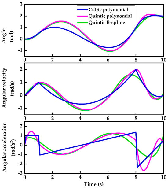
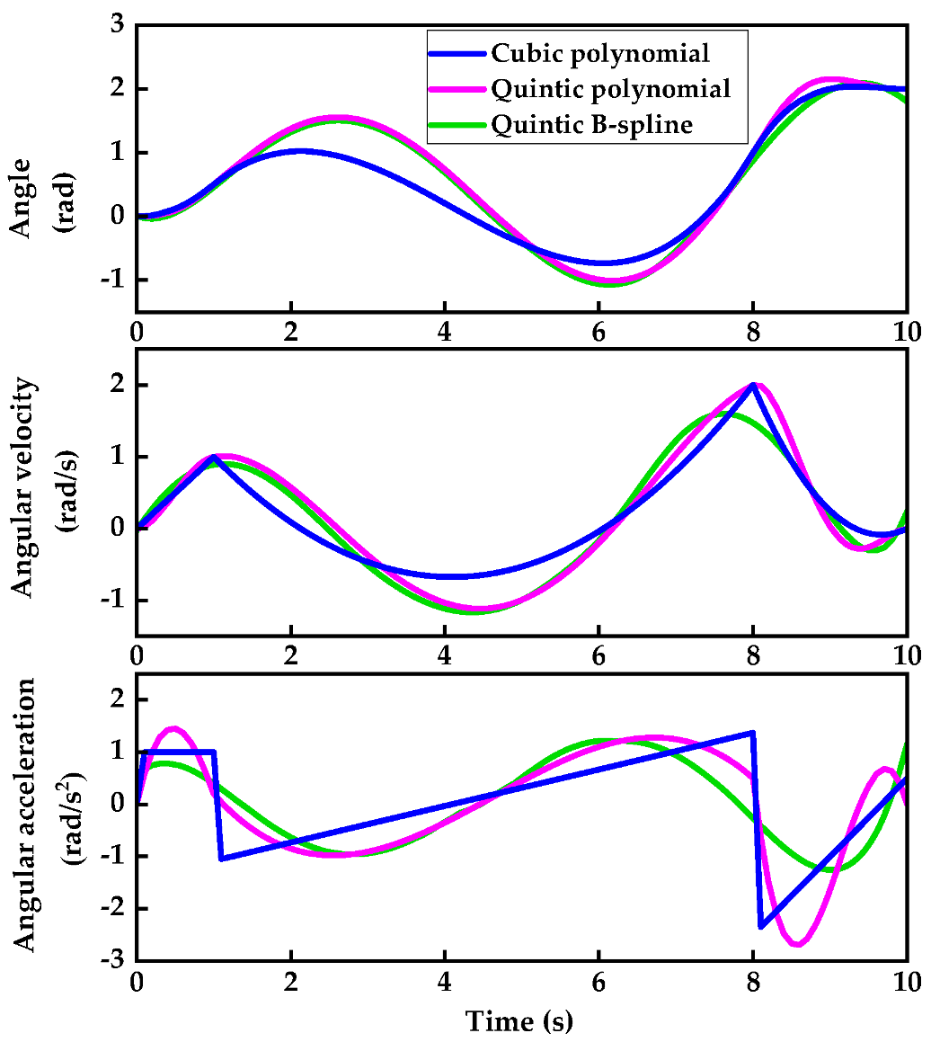
A quintic B-spline (k = 5) is selected in this study. This degree satisfies the boundary constraints for position, velocity, and acceleration at both ends while ensuring C4 continuity at the via-points, thus guaranteeing continuous angular acceleration without abrupt jumps. To verify the algorithmic superiority, the interpolation performances of the cubic polynomial [39], quintic polynomial [40], and quintic B-spline [41] are compared. The overall initial joint vector of the manipulator is set to [π/6, 0, 2π/3, π/3, 0, 0], and the target joint vector is [π/2, π/6, 0, 0, −π/2, π/6]. The initial and terminal velocities and accelerations are constrained to zero, the planning time is set to 10 s, and the sampling period is 0.1 s. Joint 6 is extracted as a representative, and its trajectory comparisons under the three algorithms are shown in Figure 7.
Figure 7.
Comparison of angle, angular velocity, and angular acceleration trajectories for Joint 6 using cubic polynomial, quintic polynomial, and quintic B-spline interpolation algorithms.
Figure 7 shows that the angular acceleration of the cubic polynomial exhibits distinct step jumps at the via-points, which easily induces flexible vibrations in the manipulator. Compared with the quintic polynomial, the quintic B-spline provides the smoothest and most natural transitions for velocity and acceleration at the via-points. Therefore, the quintic B-spline interpolation is the most suitable for the high-precision obstacle avoidance trajectory planning in this study.
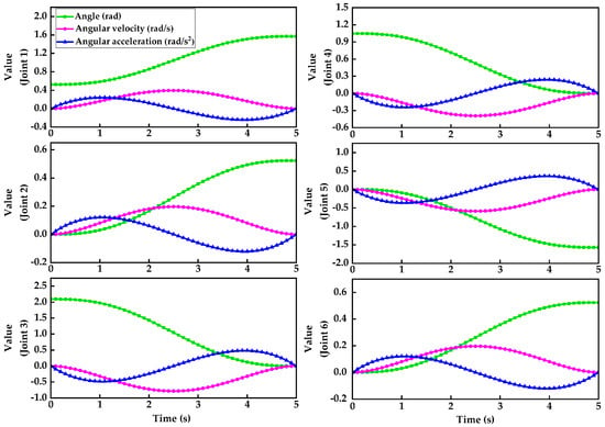
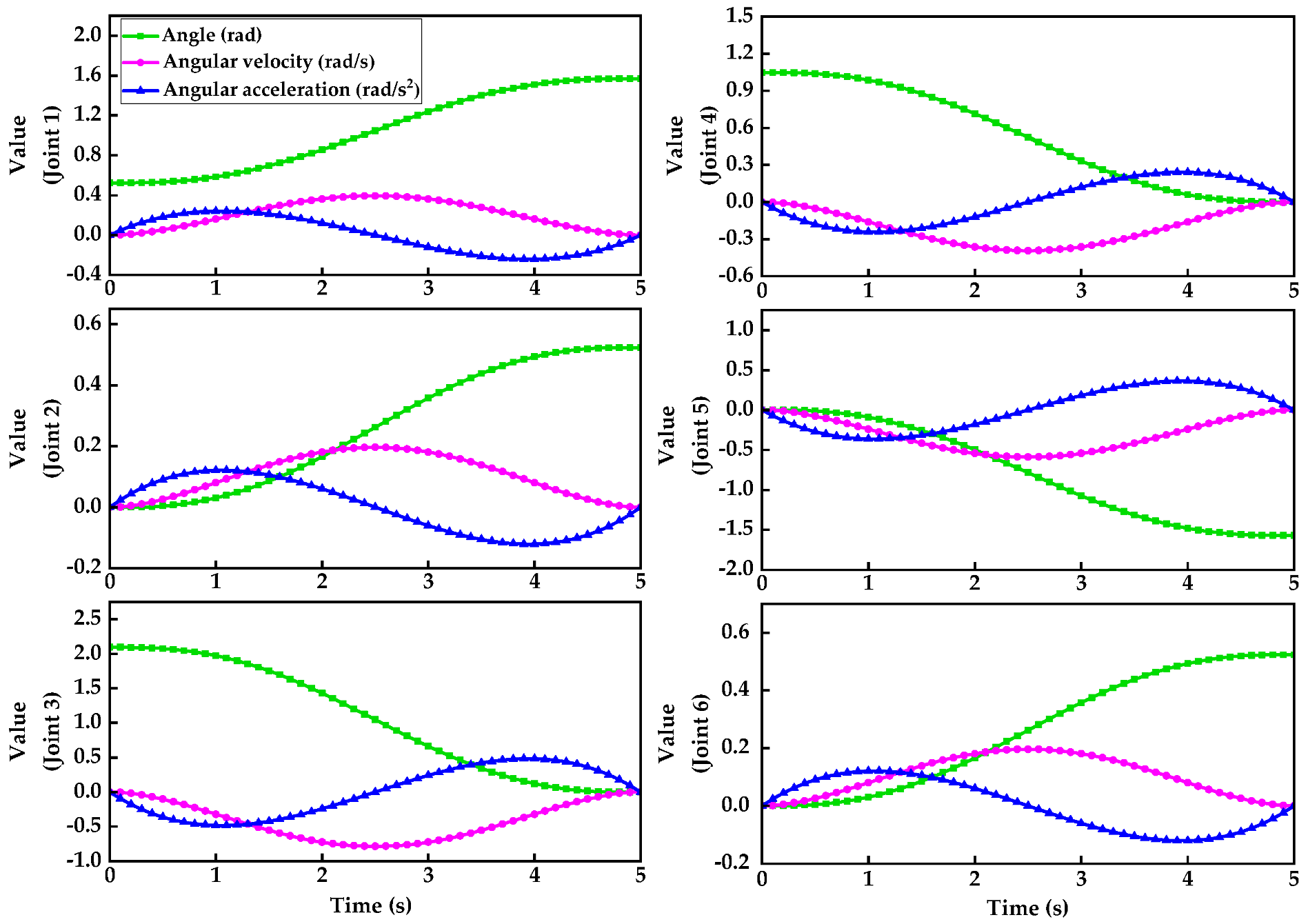
In MATLAB, the end-effector start and target positions are normalized to (130/200, −50/200, −25/200) and (130/200, 50/200, −25/200), respectively. The proposed Adaptive RRT* algorithm is then utilized for obstacle avoidance path planning to obtain collision-free discrete points in Cartesian space. To prevent abrupt joint velocity changes caused by direct workspace interpolation, inverse kinematics is applied to map these points into the joint space. Subsequently, a quintic B-spline interpolation algorithm is employed for time-parameterized trajectory planning. Finally, smooth, continuous trajectory curves for the angles, angular velocities, and angular accelerations of the six joints are generated, as shown in Figure 8.
Figure 8.
Trajectory curves of angle, angular velocity, and angular acceleration for the six joints under the obstacle avoidance path.
As seen in Figure 8, the angle, velocity, and acceleration curves of all six joints are smooth, continuous, and free of abrupt changes, with both velocity and acceleration accurately approaching zero at the initial and terminal moments. This demonstrates that the manipulator exhibits excellent kinematic smoothness during obstacle avoidance operations, effectively guaranteeing its high-precision positioning and efficient execution in confined spaces.
4. ESO-MPC-Based Trajectory-Tracking Control
To improve tracking accuracy under external disturbances and parameter uncertainties, an ESO-MPC-based controller is proposed and validated through both simulations and experiments.
4.1. Design of the ESO-MPC Controller
Based on the Lagrange method, the dynamic equation of the 6-DOF manipulator system can be expressed as
where , , and are the joint angle, angular velocity, and angular acceleration vectors, respectively; is the positive definite symmetric inertia matrix; is the Coriolis and centrifugal force matrix; is the gravity torque vector; and is the joint torque vector.
To better align with the actual physical system, by incorporating the motor dynamics and transmission errors, the system dynamics can be extended to
where , , and are the angle, angular velocity, and angular acceleration vectors of the joint motors, respectively; is the moment of inertia matrix of the joint motors; is the viscous friction coefficient matrix; is the stiffness vector; is the friction torque vector; is the transmission error vector; and N is the reduction ratio of the joint reducers, which is set to N = 100 in this study.
By eliminating the internal coupling terms from Equation (10), the comprehensive dynamic equation of the system can be derived as
Due to measurement errors and environmental factors, uncertainties inevitably exist in the parameters of the manipulator’s dynamic model. Therefore, the actual model parameters are decomposed into nominal terms and error terms:
where , , and are the nominal model parameters, while , , and are the model parameter errors.
The total lumped disturbance term De, caused by parameter perturbations, unmodeled dynamics, and external disturbances, is defined as
According to Equations (11)–(13), the dynamic model of the manipulator can be rewritten as
Based on the design principle of ESO, the system states are defined as x1 = q and , and an extended estimated state x3 is defined to lump the known and unknown disturbances:
Setting the input term h = τm, the state-space equation of the manipulator’s dynamic model can be expressed as
where r(t) is the derivative of the unknown lumped disturbance term, and y is the system output.
Let f1, f2, and f3 be the estimated values of x1, x2, and x3, respectively. The observation error is defined as e1 = f1 − x1. To reduce computational complexity and facilitate practical microcontroller deployment, the ESO is designed as follows:
where λ1, λ2, and λ3 are the observer gain coefficients. Using the bandwidth parameterization method, they are set as λ1 = 3ω0, λ2 = 3ω02, and λ3 = 3ω03, where ω0 is the observer bandwidth.
By substituting the uncertainty term in Equation (16) with the estimated value f3, the system state model can be linearized as
where the state vector is , and the virtual control input vector is . The coefficient matrices are defined as and , where I6×6 and 06×6 denote the 6 × 6 identity matrix and zero matrix, respectively.
At t = k, according to the forward Euler method, the discrete-time state-space model of the manipulator system can be expressed as
where Ag and Bg are the discrete coefficient matrices satisfying Ag = I + ATs and Bg = BTs, with Ts being the system sampling period and I being the 12 × 12 identity matrix.
Assume Np is the prediction horizon and Nc is the control horizon. It is assumed that the control input vector remains constant after Nc steps within the prediction horizon, i.e.,
At time k, given an input sequence and the current state x(k), the multi-step prediction of the system state over a future period based on Equation (19) can be organized into a matrix form:
where the predicted state sequence is ; matrix ; and matrix J is recursively derived from Ag and Bg.
Assuming the desired state sequence of the manipulator at time k is , the state tracking error sequence Ek is
To achieve high-precision trajectory tracking, a quadratic cost function Rc is designed as follows:
where wx is the state tracking error weight matrix, and wu is the control input weight matrix. Substituting Equation (21) into Equation (22), Rc can be expanded as
After expanding and omitting the constant terms that have no effect on the derivative of the optimal control law, the cost function is simplified to
Let the quadratic-term matrix be and the linear-term column vector be . Equation (25) can then be converted into a standard quadratic expression:
Meanwhile, the physical operation of the manipulator system must satisfy the following state and control input constraints:
Combining with Equation (21), the constraints can be expanded as
Synthesizing Equations (26) and (28), the model predictive control problem is rigorously transformed into a quadratic programming (QP) problem with linear constraints:
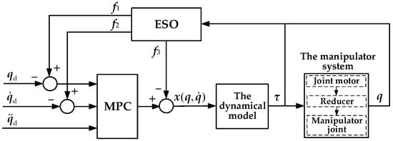
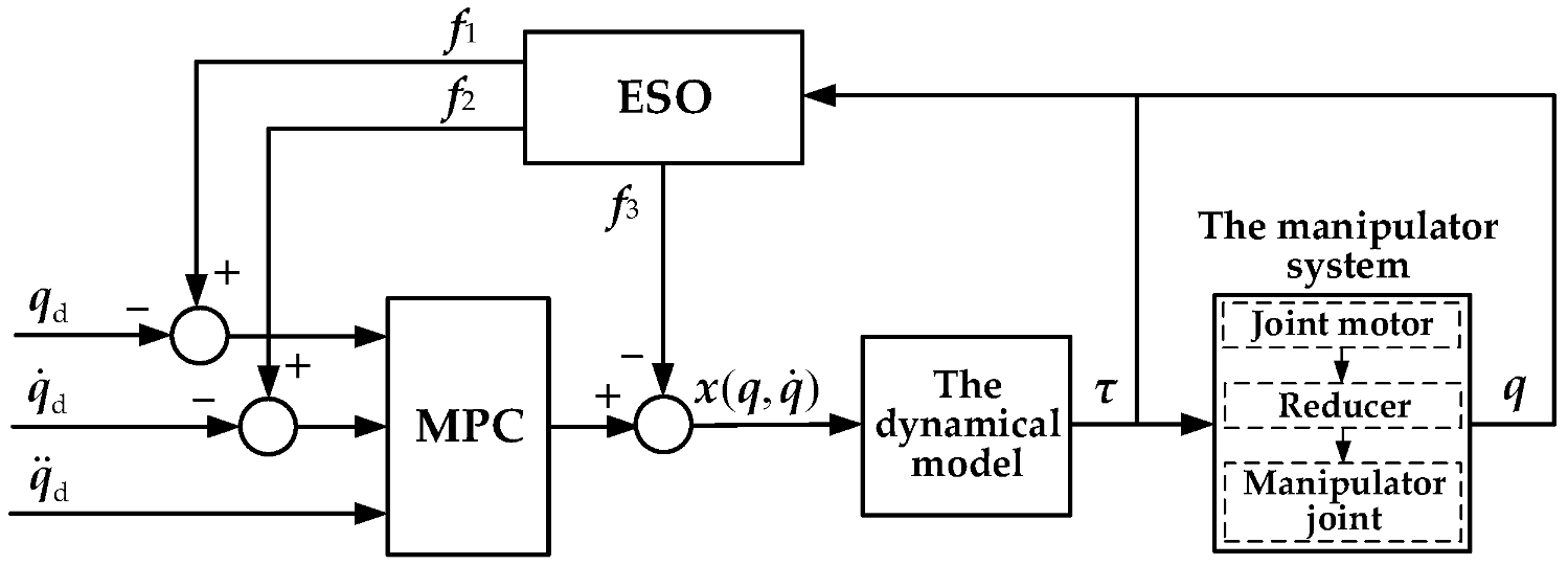
By solving Equation (29) online in each control cycle, the optimal control input vector sequence Uk* can be obtained. The first element of Uk* is taken as the virtual control input u(k), which is then mapped into the actual motor torque acting on the manipulator through the inverse dynamics compensation formula τ = Ma(q)[u(k) − f3], thereby achieving a rolling closed-loop trajectory-tracking control.
Figure 9 illustrates the overall control flowchart of the ESO-MPC controller. In this figure, , , and are the desired joint angle, angular velocity, and angular acceleration vectors, respectively.
Figure 9.
Control flowchart of the ESO-MPC controller.
4.2. Stability Analysis of the ESO-MPC Controller
To establish the overall stability of the proposed controller, the continuous-time ESO subsystem is first analyzed. Based on the system state and observer equations in Section 4.1, the observation error vector is defined as , where ei = fi − xi (i = 1, 2, 3). The dynamic equation of the observation error can be derived as
where A0 is the error coefficient matrix and B0 is the disturbance input vector, with their specific block matrix forms given by
Since ω0 > 0, A0 is strictly a Hurwitz matrix. Constructing a positive-definite quadratic Lyapunov function , for any given positive-definite symmetric matrix Q0, there exists a positive-definite symmetric matrix P0 satisfying the continuous-time Lyapunov equation:
Taking the derivative of V1(t) along the system trajectory yields
Assuming the rate of change in the lumped disturbance in the physical system is bounded, i.e., , and utilizing the matrix norm and inequality scaling, Equation (33) can be transformed into
where λmin(Q0) is the minimum eigenvalue of Q0. From Equation (34), it is evident that when the observation error satisfies , is guaranteed. According to Lyapunov’s theorem, the observation error of the ESO is uniformly ultimately bounded, and the error bound can be exponentially compressed by increasing ω0.
Subsequently, the stability of the discrete-time MPC subsystem is evaluated. Defining the state tracking error at time k as , the optimal cost function value obtained by solving Equation (29) at time k is selected as the Lyapunov candidate function:
Since wx > 0 and wu ≥ 0, it is easy to verify that V2(k) is a positive-definite function, i.e., V2(k) ≥ 0, and the equality holds if and only if e(k) = 0 and Uk* = 0. Under the standard prediction horizon recursive framework, a feasible control sequence at time k + 1 can be constructed by shifting the optimal control sequence at time k one step forward and appending the terminal element. Since the cost of the optimal solution is no greater than that of any feasible sequence, the difference in the Lyapunov function satisfies
Because wx > 0, for any non-zero tracking error sequence, ΔV2(k) < 0 always holds, demonstrating that the closed-loop MPC subsystem possesses global asymptotic stability.
Building upon the stability of both subsystems, the overall closed-loop ESO-MPC system is essentially a continuous–discrete hybrid dynamic system with a sampling period of Ts. Constructing a composite Lyapunov function,
Based on the Separation Principle, within the continuous-time interval , V2(k) remains constant due to the zero-order hold of the control input, whereas V1(t) strictly decays with the continuous state estimation. At the discrete sampling instant t = kTs, V2(k) experiences a strict discrete decay (Equation (36)), and since the ESO state estimation exhibits no discrete jumps, V1(t) remains continuous.
Therefore, V(t,k) strictly decreases monotonically across the global time domain. By properly configuring ω0 to ensure that the ESO converges significantly faster than the MPC, observation error perturbations are prevented from compromising the robustness bound of the MPC. Consequently, the ESO-MPC system achieves global asymptotic stability and high anti-disturbance robustness.
4.3. Trajectory-Tracking Simulation on a Scaled-Down Model
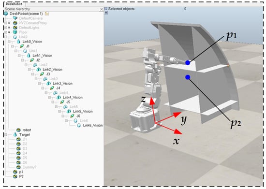
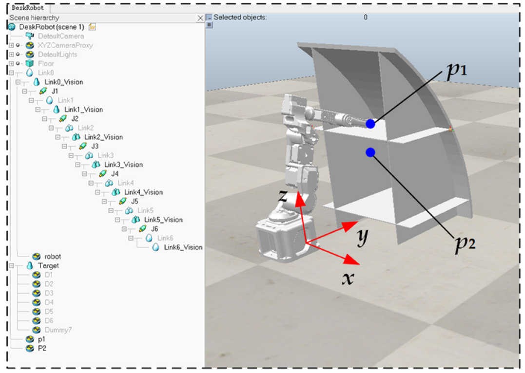
The scaled-down 3D models of the 6-DOF manipulator and the ship compartments were constructed in SolidWorks 2023 and imported into the CoppeliaSim simulation platform, as shown in Figure 10. The workspace was set to 1500 mm × 1500 mm, the vertical distance between the manipulator base and the bottom of the compartments was set to 150 mm, and the global world coordinate system coincided with the manipulator’s base coordinate system. The initial position of the manipulator’s end-effector was set to p1 = (0, 300, 250) mm, and the target position was set to p2 = (−100, 250, 200) mm.
Figure 10.
The manipulator model and ship compartment model in the CoppeliaSim V4.6.0.
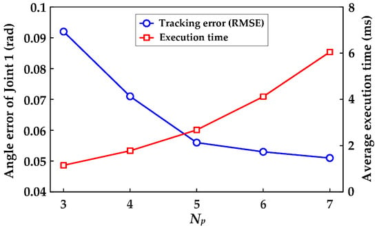
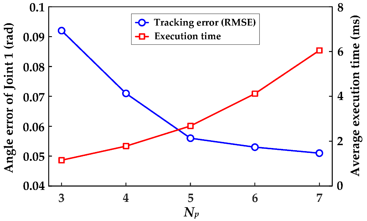
To determine the optimal configuration of the controller, a sensitivity analysis was conducted on Np, and empirical tuning was performed on ω0, Nc, wx, and wu in combination with physical constraints. First, ω0 involves a trade-off between state estimation speed and noise suppression. An excessively small value leads to a lag in disturbance compensation, while an overly large value amplifies high-frequency noise and induces torque chattering. To balance the requirements for rapid estimation and noise immunity, it was set to ω0 = 20 rad/s. Second, Figure 11 illustrates the impact of different Np values on tracking accuracy and single-step execution time. When Np increased from 3 to 5, the Root Mean Square Error (RMSE) significantly decreased to 0.056 rad; when it further increased to 6 or 7, the improvement in accuracy was minimal, whereas the execution time surged linearly. Weighing the control accuracy against the real-time computational limits of the microprocessor, Np = 5 was selected, and Nc was set to 5. Finally, to ensure high-precision tracking and avoid motor saturation, the weight matrices were directly tuned to wx = diag(5, 4.5, 3, 5, 2, 4) and wu = diag(0.01, 0.01, 0.01, 0.01, 0.01, 0.01) based on the physical inertia characteristics of each manipulator joint.
Figure 11.
Sensitivity analysis of Np.
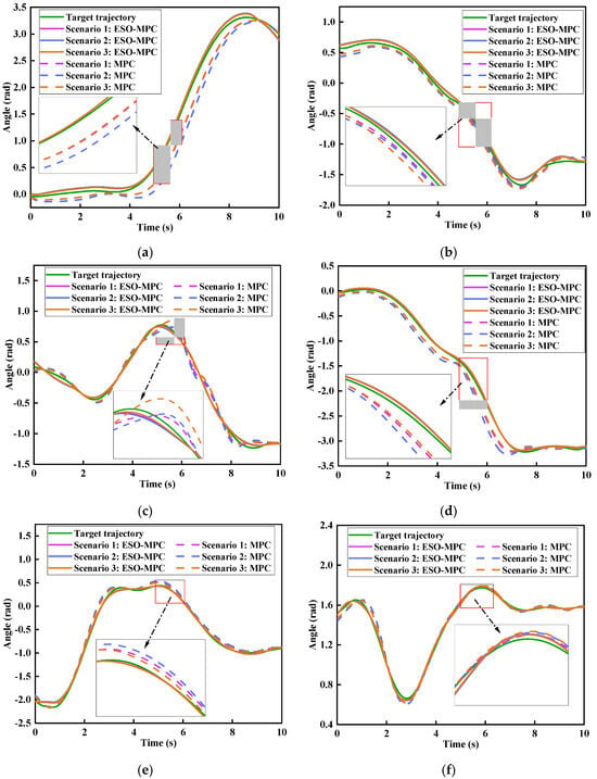
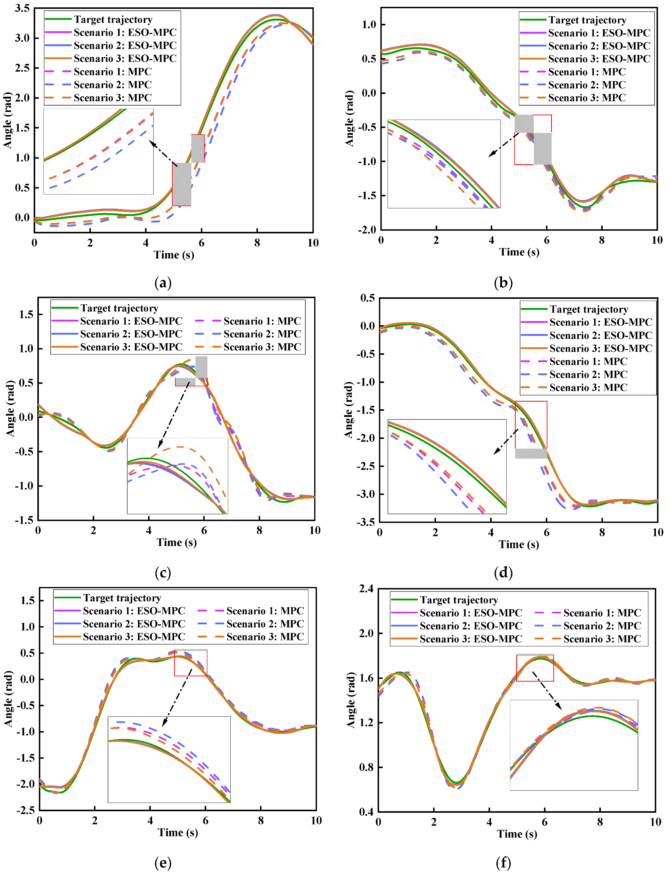
The end-effector path is planned using the Adaptive RRT* algorithm described in Section 3. Target joint trajectories are then generated by solving the inverse kinematics at path points and applying quintic B-spline interpolation. The system sampling time was set to Ts = 0.01 s. To comprehensively evaluate the trajectory-tracking performance and robustness of ESO-MPC and traditional MPC in confined spaces, three typical working scenarios with a total duration of 10 s were designed: Scenario 1 was the nominal condition, where the manipulator executed the trajectory-tracking task under ideal standard physical parameters; Scenario 2 was the parameter uncertainty condition, where the mass of all links was increased by 20% while the controller maintained the nominal model, to simulate modeling errors and sudden payload variations; Scenario 3 was the transient external-disturbance condition, where a step disturbance torque with an amplitude of 0.6 N·m and a duration of 0.2 s was injected into Joint 3 at t = 5.0 s, to test the impact resistance and recovery capabilities. The joint angle tracking results under the aforementioned three scenarios are shown in Figure 12.
Figure 12.
Joint angle tracking trajectories of the manipulator under three scenarios: (a) Joint 1; (b) Joint 2; (c) Joint 3; (d) Joint 4; (e) Joint 5; (f) Joint 6.
As shown in Figure 12, in Scenario 1, each joint effectively tracks the target trajectory under both MPC and ESO-MPC. Notably, the ESO-MPC tracking trajectory exhibits tighter alignment and superior steady-state accuracy. In Scenario 2, the increased link mass introduces dynamic model mismatch. Due to the lack of precise compensation, MPC results in significant phase lag and steady-state deviation; conversely, ESO-MPC effectively estimates and compensates for internal parameter perturbations, maintaining high consistency between actual and target trajectories and demonstrating robustness against parameter variations. In Scenario 3, when facing a sudden step disturbance at t = 5.0 s, Joint 3 under MPC rapidly deviates and recovers slowly. In contrast, ESO-MPC significantly suppresses the deviation amplitude and achieves rapid re-convergence. This indicates that ESO-MPC can proactively compensate for external torques in real-time, providing the system with enhanced impact resistance and dynamic recovery capabilities.
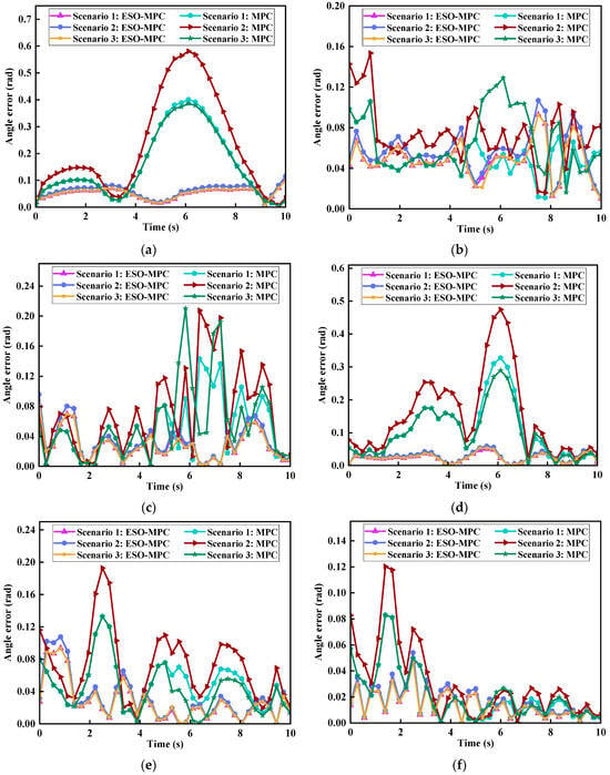
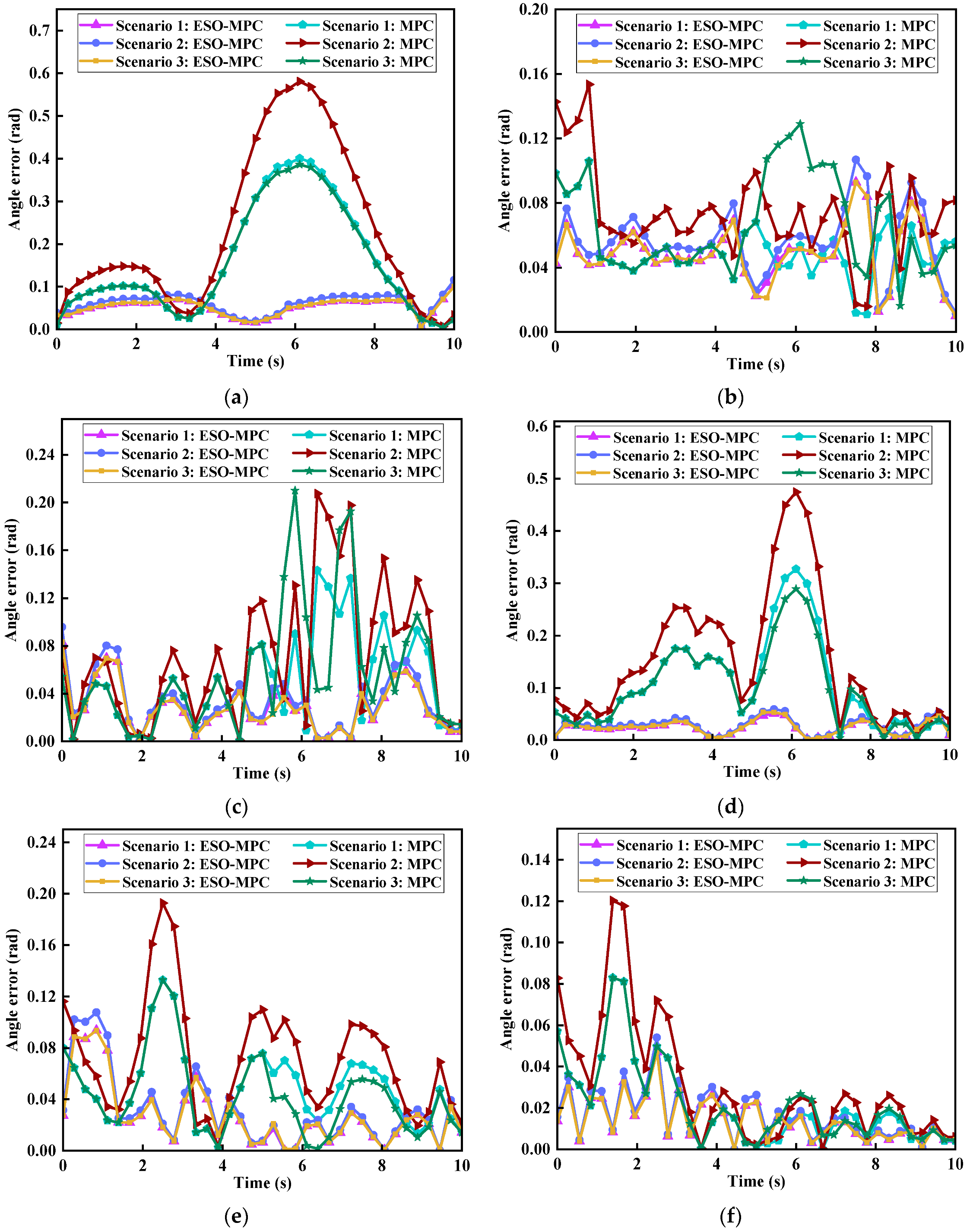
To visually evaluate the trajectory-tracking performance, Figure 13 illustrates the absolute tracking error curves of each joint across the three scenarios.
Figure 13.
Joint angle tracking error curves of the manipulator under ESO-MPC and MPC in three scenarios: (a) Joint 1; (b) Joint 2; (c) Joint 3; (d) Joint 4; (e) Joint 5; (f) Joint 6.
As shown in Figure 13, in Scenario 1, the error amplitude under ESO-MPC is significantly lower than that under MPC. In Scenario 2, in the presence of parameter perturbations, the errors under MPC control exhibit obvious steady-state offsets and divergence; in contrast, relying on real-time disturbance compensation, ESO-MPC suppresses the errors within an extremely narrow band. In Scenario 3, facing transient external disturbances, the error peaks under MPC control surge drastically and exhibit a sluggish regulation process; conversely, the disturbance-induced peaks under ESO-MPC control are substantially attenuated and rapidly recover to a steady state. This demonstrates that the ESO-MPC system features a smaller overshoot and superior dynamic recovery capabilities.
For further quantitative evaluation, Table 4 summarizes the percentage reductions in trajectory-tracking error metrics (Maximum Absolute Error (MaxAE), Mean Error (ME), and RMSE) achieved by ESO-MPC compared to traditional MPC in each scenario. In Scenario 1, the various error metrics under ESO-MPC were reduced by 5.78% to 84.35% compared to MPC, effectively improving the baseline tracking accuracy. In Scenarios 2 and 3, the tracking accuracy under traditional MPC deteriorated significantly; meanwhile, relying on the precise compensation of lumped disturbances, ESO-MPC maintained the reduction percentages of all error metrics between 25.27% and 87.59%. Quantitative data strongly confirm that ESO-MPC not only possesses extremely high steady-state accuracy but also exhibits outstanding anti-disturbance robustness in complex dynamic environments.
Table 4.
Percentage reductions in trajectory-tracking errors achieved by ESO-MPC compared to traditional MPC.
4.4. Experimental Validation on a Scaled-Down Platform
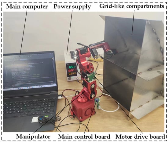
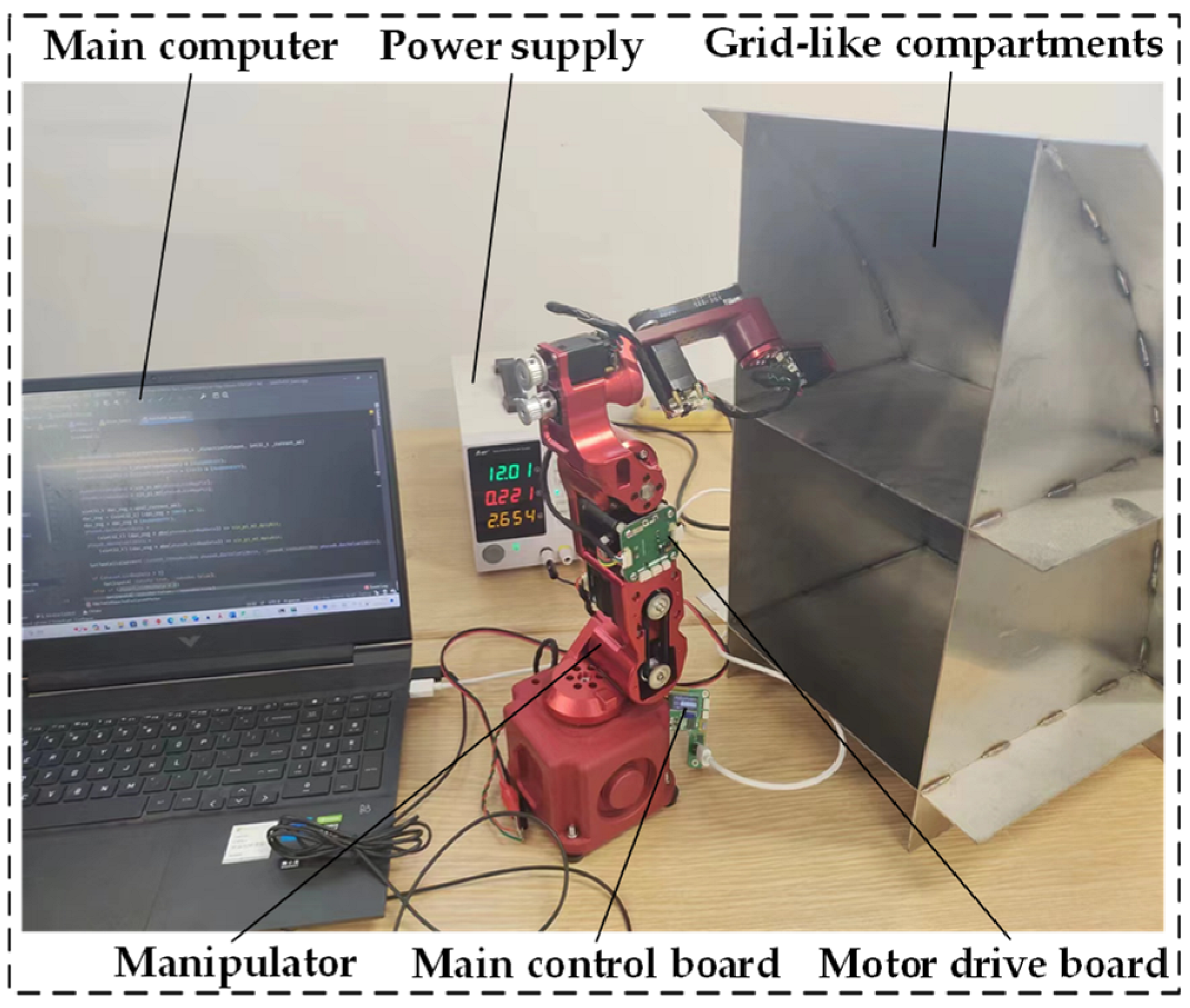
To verify the real-time operational capability and disturbance rejection performance of the proposed ESO-MPC controller in a physical system, a scaled-down experimental platform for 6-DOF manipulator trajectory tracking was constructed, as shown in Figure 14. The control system operates as follows: the core ESO-MPC algorithm is deployed on the upper computer, which in real-time collects data from each joint encoder and solves optimization instructions online at a control cycle of Ts = 10 ms. Subsequently, the instructions are transmitted to the main control board and motor drive boards via a high-speed communication bus to complete the physical closed-loop control.
Figure 14.
A scaled-down experimental platform for trajectory tracking.
Regarding the computational burden of the system, online statistics were conducted over 1000 continuous control cycles. The results indicate that with a prediction horizon of Np = 5, the average time for a single-step state update of the ESO is only 0.05 ms, while the average total computational time for a single control cycle is 2.8 ms. Under the worst-case scenario, the maximum total time does not exceed 3.5 ms, which is well below the control cycle threshold of 10 ms. This fully validates the reliable real-time computational capability of the proposed controller.
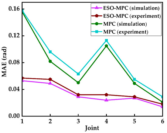
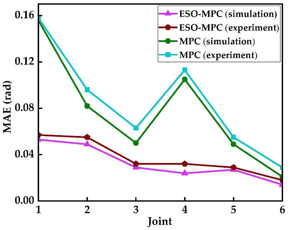
The target trajectory from Section 4.3 is used as the reference for this experiment. Figure 15 compares the tracking performance (measured by Mean Absolute Error, MAE) of each joint under ESO-MPC and traditional MPC across both the simulation environment (Scenario 1) and physical experiments.
Figure 15.
Comparison of MAE values for joint tracking trajectories under ESO-MPC and MPC in simulation and physical experiments.
As illustrated in Figure 15, the MAE under both control strategies is higher in the experiments than in the simulations due to unmodeled disturbances in the physical system. However, when subjected to equivalent disturbances, the tracking error under traditional MPC deteriorated significantly. In contrast, the error under ESO-MPC increased only slightly, and its overall MAE remained far superior to that of the traditional MPC. These results demonstrate that the proposed controller effectively estimates and compensates for disturbances in real-time, exhibiting superior robustness and control precision during trajectory tracking.
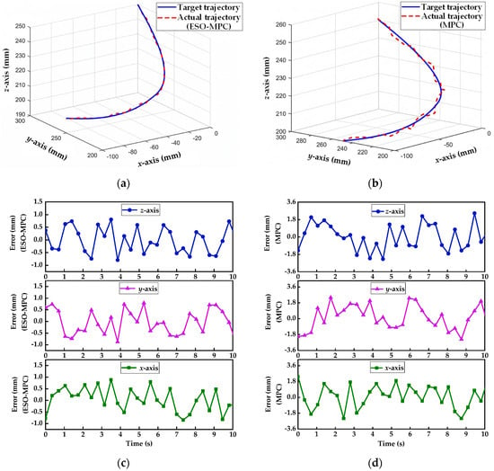
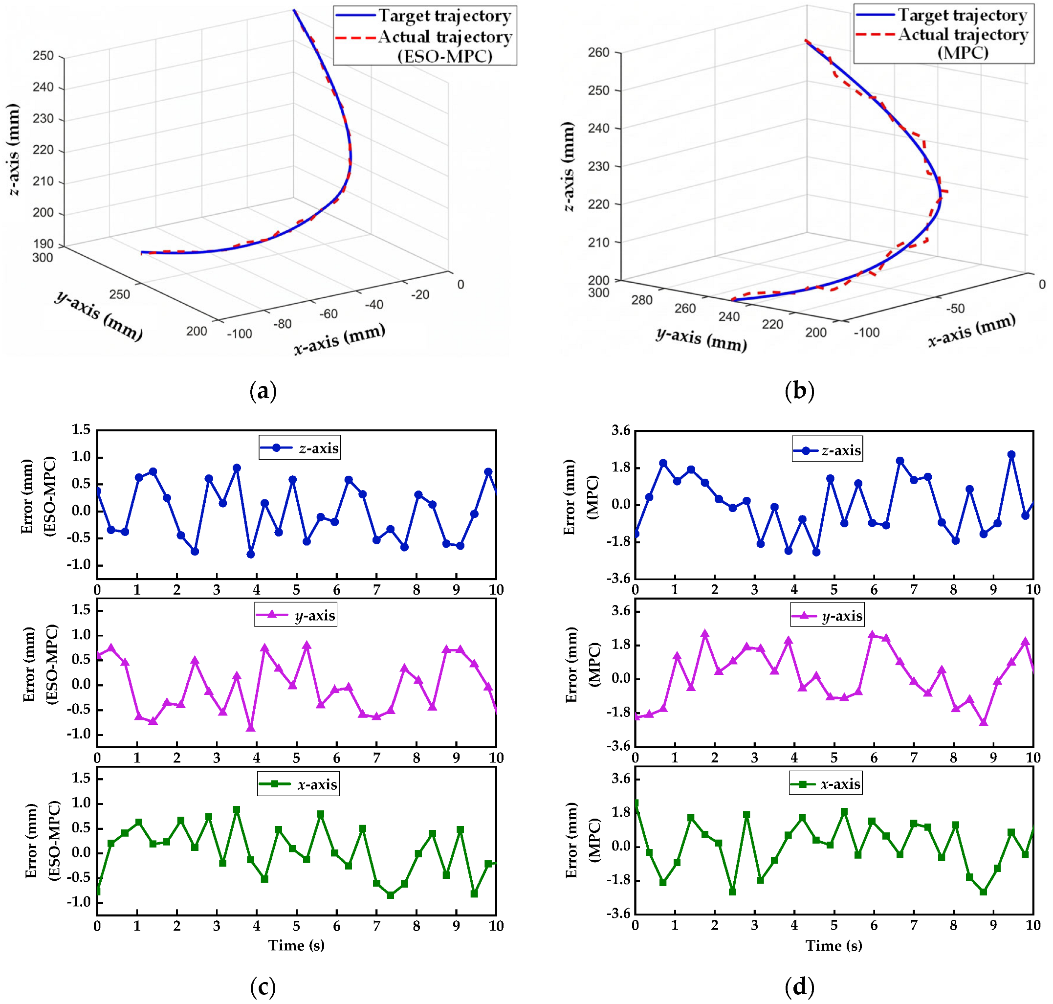
Figure 16 presents the spatial trajectory-tracking curves and error dynamics of the end-effector.
Figure 16.
Comparison of end-effector spatial trajectory-tracking performance: (a) ESO-MPC trajectory; (b) MPC trajectory; (c) ESO-MPC tracking error; (d) MPC tracking error.
From Figure 16a,b, it is observed that the actual trajectory under ESO-MPC fits the target more closely, with no significant lag at the inflection points. Data from Figure 16c,d show that the maximum absolute tracking errors for the end-effector under ESO-MPC along the x, y, and z axes are 0.88 mm, 0.85 mm, and 0.89 mm, respectively, which are substantially smaller than those of the traditional MPC (2.41 mm, 2.39 mm, and 2.47 mm). Consequently, the proposed ESO-MPC controller achieves superior high-precision tracking performance.
4.5. Engineering Feasibility Verification Based on a Full-Scale Model
To validate the applicability of the proposed Adaptive RRT* algorithm and the ESO-MPC controller in realistic industrial scenarios, this section constructs a full-scale, 3D model of ship compartments with physical dimensions of 1500 × 1500 × 2250 mm. A standard industrial manipulator, the ABB IRB 2600-12/1.85, is employed for simulation.
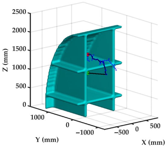
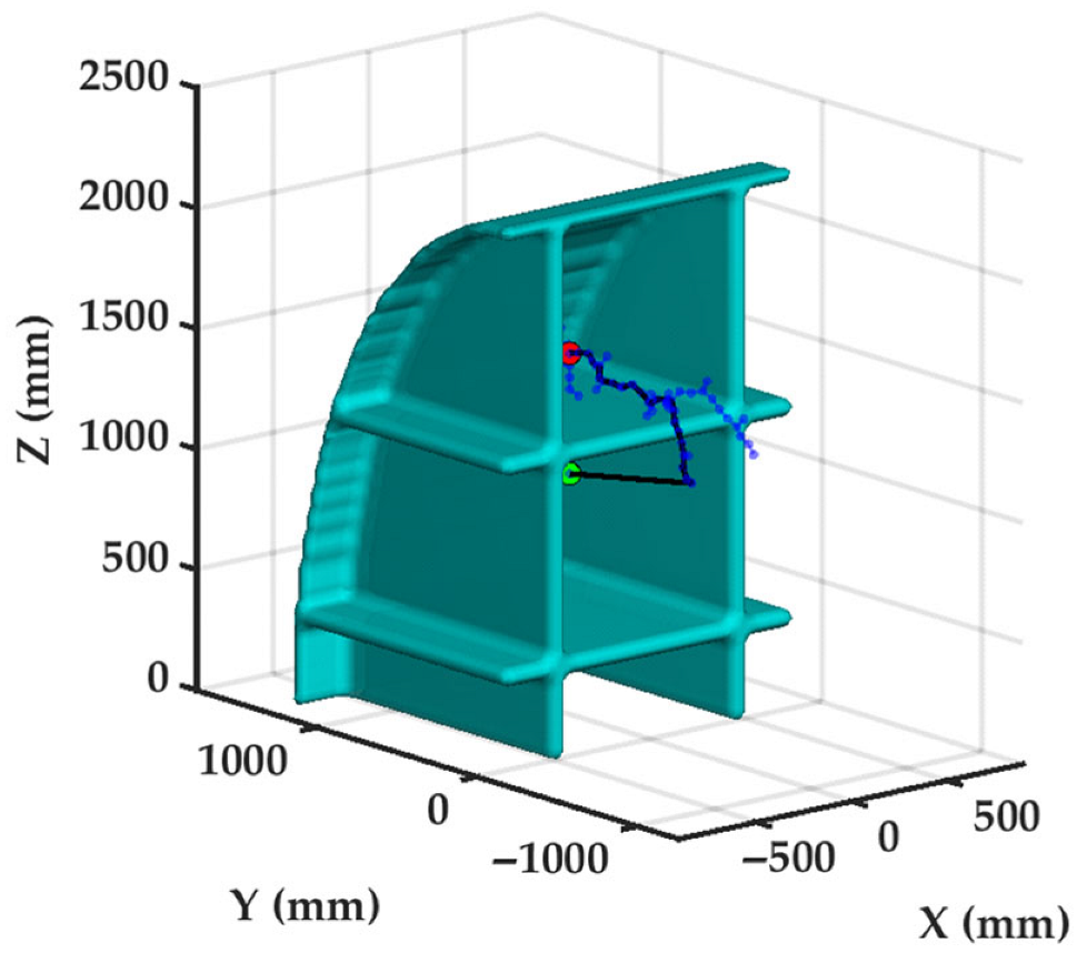
The MATLAB simulation environment and parameter settings are as follows: the continuous search space is set to 2000 × 2500 × 2500 mm; the coordinates for the start and target points of the end-effector are (0, 500, 1500) mm and (0, 500, 1000) mm, respectively; and the maximum number of iterations for the algorithm is limited to 10,000. A total of 100 independent repetitive experiments were conducted using the Adaptive RRT* algorithm, with a representative obstacle avoidance planned path shown in Figure 17.
Figure 17.
Obstacle avoidance path planned by Adaptive RRT* in a full-scale ship compartment environment.
The simulation results demonstrate that in the full-scale scenario, the Adaptive RRT* algorithm achieves an average path length of 1933.39 mm, a mean planning time of 0.53 s, and an average of 63.00 tree nodes, while maintaining a 100% success rate. These results strongly confirm that despite the substantial increase in workspace scale, the algorithm remains capable of efficiently generating collision-free and topologically optimized paths, demonstrating excellent reliability and adaptability suitable for industrial applications in large-scale environments.
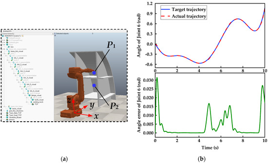
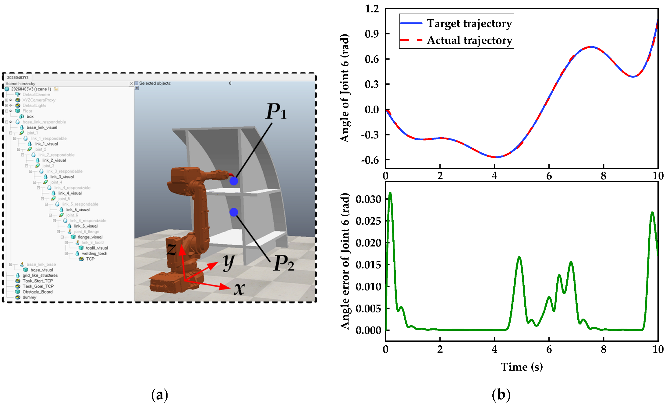
Furthermore, the ABB IRB 2600 manipulator and the full-scale ship compartment model are imported into the CoppeliaSim simulation platform. As shown in Figure 18a, the workspace is set to 5000 × 5000 mm, with the vertical distance between the manipulator base and the bottom of the compartments set to 650 mm. The start and target positions of the end-effector are defined as P1 = (0, 1150, 1500) mm and P2 = (0, 1150, 1000) mm, respectively. The key parameters of the ESO-MPC controller are set as follows: ω0 = 20 rad/s, Np = Nc = 5, wx = diag(5, 4.5, 3, 5, 2, 4), wu = diag(0.01, 0.01, 0.01, 0.01, 0.01, 0.01), and Ts = 0.01 s. The target trajectory for Joint 6 is generated based on the method described in Section 3, and the manipulator is driven to execute the trajectory-tracking task under nominal physical parameters. The results are presented in Figure 18b.
Figure 18.
Trajectory-tracking simulation of Joint 6 in the full-scale scenario: (a) Manipulator and ship compartment model in CoppeliaSim; (b) angle trajectory-tracking results of Joint 6.
As shown in Figure 18b, under the control of the ESO-MPC, the actual trajectory of Joint 6 highly coincides with the target trajectory, with an MAE of only 4.08 × 10⁻³ rad. The simulation results confirm that the proposed planning algorithm and control framework exhibit excellent obstacle avoidance planning capabilities and high-precision trajectory-tracking performance, effectively meeting the operational requirements of actual industrial environments.
5. Conclusions
To address the challenges of obstacle avoidance planning and high-precision tracking for 6-DOF manipulators within constrained ship grid-like compartment environments, this paper proposes a complete planning and control framework. The main conclusions are as follows:
(1) An accurate kinematic model of a scaled-down 6-DOF manipulator was established, providing the mathematical foundation for trajectory planning and tracking control.
(2) An Adaptive RRT* for obstacle avoidance in constrained environments was developed. By introducing a multi-source state feedback mechanism, the algorithm enables dynamic adjustment of target bias and greedy expansion probabilities. Simulations indicate that the average path length (374.28 mm) is reduced by 29.5% compared to Informed RRT* (530.80 mm). The average planning time (0.30 s) is 64.7% shorter than that of RRT-Connect (0.85 s), and the average node count (50.83) decreases by 28.6% compared to RRT-Connect (71.16), with a 100% planning success rate. Furthermore, quintic B-spline interpolation ensures joint trajectory continuity at the position, velocity, and acceleration levels.
(3) An ESO-MPC controller with active disturbance rejection was designed and validated. Simulations show that under nominal conditions, tracking error metrics of ESO-MPC are reduced by 5.78–84.35% compared to MPC. Under a 20% link mass perturbation, the controller eliminates phase lag, achieving an error reduction of 25.27–87.59%. Under a 0.6 N·m step torque disturbance, it maintains the error reduction at 27.14–81.48% through real-time compensation of lumped disturbances, exhibiting excellent robustness and dynamic recovery.
(4) The control scheme was verified on a scaled-down experimental platform. Results show that although experimental errors are slightly higher than simulation values due to unmodeled dynamics and disturbances in the actual system, ESO-MPC exhibits stronger anti-interference capability, with MAE metrics significantly superior to MPC. Under ESO-MPC, the maximum tracking errors of the end-effector along the x, y, and z axes are 0.88 mm, 0.85 mm, and 0.89 mm, respectively, which are markedly lower than the 2.41 mm, 2.39 mm, and 2.47 mm corresponding to MPC. This confirms that the proposed control scheme possesses high tracking precision and reliability.
(5) Engineering feasibility was verified using full-scale models. In simulations, the Adaptive RRT* algorithm achieves a 100% success rate, with an average path length, planning time, and node count of 1933.39 mm, 0.53 s, and 63.00, respectively. Under ESO-MPC, the Joint 6 angular trajectory highly coincides with the target, yielding an MAE of 4.08 × 10⁻³ rad. This demonstrates the framework’s capability for efficient obstacle avoidance and stable tracking at industrial scales.
In summary, the proposed framework demonstrates superior performance across algorithm comparisons, scaled-model simulations and physical experiments, as well as full-scale model verifications. It effectively addresses high-precision obstacle avoidance and trajectory tracking in complex constrained environments, offering significant engineering value.
6. Limitations and Future Work
This study has two primary limitations: physical validation was restricted to a scaled-down educational robot (with industrial-scale performance verified only via simulation), and the research scope is strictly confined to spatial motion planning and tracking control, rather than the technological process of welding itself. To address these constraints, future work will focus on deploying the proposed algorithms on physical, industrial-grade manipulators in real-world confined settings. Additionally, we will integrate a dynamic perception module to enable real-time trajectory adaptation in complex, unstructured environments.
Author Contributions
Conceptualization, Q.H.; methodology, K.Z. and Q.H.; software, L.L.; validation, K.Z. and Z.W.; formal analysis, H.L.; investigation, K.Z.; resources, Q.H.; data curation, Z.W.; writing—original draft preparation, K.Z.; writing—review and editing, Q.H. and K.Z.; visualization, Z.W.; supervision, L.L.; project administration, Q.H.; funding acquisition, Q.H. All authors have read and agreed to the published version of the manuscript.
Funding
The authors gratefully acknowledge the National Natural Science Foundation of China, coded 52305061, the Jiangsu Province Industry-University-Research Cooperation coded BY20240463, and the Science and Technology Project of Jiangsu Provincial Administration for Market Regulation in 2025 coded KJ2025020.
Data Availability Statement
Data are contained within the article.
Conflicts of Interest
The authors declare no conflicts of interest.
Abbreviations
The following abbreviations are used in this manuscript:
| 6-DOF | Six Degrees of Freedom |
| RRT* | Rapidly exploring Random Tree Star |
| ESO | Extended State Observer |
| MPC | Model Predictive Control |
| APF | Artificial Potential Field |
| SIO | Swarm Intelligence Optimization |
| RRT | Rapidly exploring Random Tree |
| PSO | Particle Swarm Optimization |
| WOA | Whale Optimization Algorithm |
| DDPG | Deep Deterministic Policy Gradient |
| TD3 | Twin Delayed Deep Deterministic Policy Gradient |
| ILC | Iterative Learning Control |
| PID | Proportional–Integral–Derivative |
| QPSO | Quantum Particle Swarm Optimization |
| NDO | Nonlinear Disturbance Observer |
| DRL | Deep Reinforcement Learning |
| DWA | Dynamic Window Approach |
| MaxAE | Maximum Absolute Error |
| ME | Mean Error |
| RMSE | Root Mean Square Error |
| MAE | Mean Absolute Error |
References
- Wang, B.C.; Hu, S.J.; Sun, L.; Freiheit, T. Intelligent welding system technologies: State-of-the-art review and perspectives. J. Manuf. Syst. 2020, 56, 373–391. [Google Scholar] [CrossRef] [Scilit]
- Liu, J.F.; Cheng, Y.F.; Jing, X.W.; Liu, X.J.; Chen, Y. Prediction and optimization method for welding quality of components in ship construction. Sci. Rep. 2024, 14, 9353. [Google Scholar] [CrossRef] [Scilit]
- Lee, D.; Ku, N.; Kim, T.W.; Kim, J.; Lee, K.Y.; Son, Y.S. Development and application of an intelligent welding robot system for shipbuilding. Robot. Comput. Integr. Manuf. 2010, 27, 377–388. [Google Scholar] [CrossRef] [Scilit]
- Feng, X.B.; Tian, W.; Wei, R.; Pan, B.W.; Chen, Y.; Chen, S.Y. Application of a wall-climbing, welding robot in ship automatic welding. J. Coast. Res. 2020, 106, 609–613. [Google Scholar] [CrossRef] [Scilit]
- Liu, Y.; Li, X.; Jiang, P.Y.; Du, Z.; Wu, Z.; Sun, B.X.; Huang, X.Y. Evolutionary multi-objective trajectory optimization for a redundant robot in Cartesian space considering obstacle avoidance. Mech. Sci. 2022, 13, 41–53. [Google Scholar] [CrossRef] [Scilit]
- Carvajal, C.P.; Andaluz, V.H.; Roberti, F.; Carelli, R. Path-following control for aerial manipulators robots with priority on energy saving. Control Eng. Pract. 2023, 131, 105401. [Google Scholar] [CrossRef] [Scilit]
- Liu, M.J.; Zhang, H.X.; Yang, J.; Zhang, T.Z.; Zhang, C.H.; Bo, L. A path planning algorithm for three-dimensional collision avoidance based on potential field and B-spline boundary curve. Aerosp. Sci. Technol. 2024, 144, 108763. [Google Scholar] [CrossRef] [Scilit]
- Elgohr, T.A.; Elazab, A.M.; Emam, Z.A.; Mostafa, G.M.; Razgan, A.M.; Kasem, M.H.; Elhadidy, S.M. Particle swarm optimization vs. whale optimization algorithm for robotic arm path planning: A controlled study on the KUKA KR4 R600. Results Eng. 2025, 28, 108299. [Google Scholar] [CrossRef] [Scilit]
- Al Ali, A.; Shi, F.J.; Zhu, H.Z. Path planning of 6-DOF free-floating space robotic manipulators using reinforcement learning. Acta Astronaut. 2024, 224, 367–378. [Google Scholar] [CrossRef] [Scilit]
- Xu, Y.H.; Kong, S.H.; Kong, X.W.; Ying, Z.X. Multi-objective trajectory optimization method for industrial robots based on improved TD3 algorithm. Sci. Rep. 2025, 15, 41970. [Google Scholar] [CrossRef] [Scilit]
- Jo, M.S.; Chung, M.; Kim, M.; Kim, H.Y. Improving path accuracy and vibration character of industrial robot arms with iterative learning control method. Int. J. Precis. Eng. Manuf. 2024, 25, 1851–1863. [Google Scholar] [CrossRef] [Scilit]
- Khan, A.T.; Li, S.; Kadry, S.; Nam, Y. Control framework for trajectory planning of soft manipulator using optimized RRT algorithm. IEEE Access 2020, 8, 171730–171743. [Google Scholar] [CrossRef] [Scilit]
- Fang, Y.; Lu, L.W.; Zhang, B.Q.; Liu, X.T.; Zhang, H.F.; Fan, D.Q.; Yang, H. Motion control of obstacle avoidance for the robot arm via improved path planning algorithm. J. Braz. Soc. Mech. Sci. Eng. 2024, 46, 727. [Google Scholar] [CrossRef] [Scilit]
- Liang, J.L.; Luo, W.G.; Qin, Y.X. Path planning of multi-axis robotic arm based on improved RRT*. Comput. Mater. Contin. 2024, 81, 1009–1027. [Google Scholar] [CrossRef] [Scilit]
- Zhao, X.X.; Wang, K.; Zhang, P.Y.; Kan, J.M. An improved RRT* path planning algorithm combining Gaussian distributed sampling and depth strategy for robotic arm of fruit-picking robot. Comput. Electron. Agric. 2026, 240, 111244. [Google Scholar] [CrossRef] [Scilit]
- Ku, X.C.; Zhu, E.; Li, S. Obstacle avoidance path planning for robotic arms using a multi-strategy collaborative bidirectional RRT* algorithm. Sensors 2026, 26, 1376. [Google Scholar] [CrossRef] [Scilit]
- Jeong, I.B.; Lee, S.J.; Kim, J.H. Quick-RRT*: Triangular inequality-based implementation of RRT* with improved initial solution and convergence rate. Expert Syst. Appl. 2019, 123, 82–90. [Google Scholar] [CrossRef] [Scilit]
- Qi, J.; Yang, H.; Sun, H.X. MOD-RRT*: A sampling-based algorithm for robot path planning in dynamic environment. IEEE Trans. Ind. Electron. 2020, 68, 7244–7251. [Google Scholar] [CrossRef] [Scilit]
- Qi, E.; Zhang, T.L.; Zhao, L.Y.; Han, F.; Ge, J.L.; Qi, Y.B.; Qi, Y.P. Research on robotic arm path planning method based on two-stage RRT* optimization algorithm. Eng. Res. Express 2025, 7, 035416. [Google Scholar] [CrossRef] [Scilit]
- Xiong, Z.H.; Hou, W.B.; Wang, C.S.; Chen, H. Classified-RRT*: Node classification RRT*-based algorithm with improved solution performance and convergence rate. Expert Syst. Appl. 2026, 296, 129118. [Google Scholar] [CrossRef] [Scilit]
- Guo, S.J.; Gong, J.J.; Shen, H.T.; Yuan, L.L.; Wei, W.; Long, Y. DBVSB-P-RRT*: A path planning algorithm for mobile robot with high environmental adaptability and ultra-high speed planning. Expert Syst. Appl. 2025, 266, 126123. [Google Scholar] [CrossRef] [Scilit]
- Cheng, X.; Zhou, J.M.; Zhou, Z.; Zhao, X.M.; Gao, J.J.; Qiao, T. An improved RRT-Connect path planning algorithm of robotic arm for automatic sampling of exhaust emission detection in Industry 4.0. J. Ind. Inf. Integr. 2023, 33, 100436. [Google Scholar] [CrossRef] [Scilit]
- Hu, Q.S.; Li, H.; Li, H.Q.; Wang, G.W.; Li, L. Optimization of control parameters for robot integrated joint modules based on an MA-BPNN model. J. Chin. Soc. Mech. Engineers. 2024, 45, 605–618. [Google Scholar]
- Hu, Q.S.; Liu, Z.F.; Yang, C.B.; Xie, F.G. Research on dynamic transmission error of harmonic drive with uncertain parameters by an interval method. Precis. Eng. 2021, 68, 285–300. [Google Scholar] [CrossRef] [Scilit]
- Azeez, M.I.; Atia, K.R. Modeling of PID controlled 3DOF robotic manipulator using Lyapunov function for enhancing trajectory tracking and robustness exploiting Golden Jackal algorithm. ISA Trans. 2024, 145, 190–204. [Google Scholar] [CrossRef] [Scilit]
- Fareh, R.; Saad, M.; Saad, M.; Bettayeb, M. Tracking trajectory in the workspace of rigid manipulators using distributed adaptive control strategy. Adv. Robot. 2016, 30, 361–373. [Google Scholar] [CrossRef] [Scilit]
- Rsetam, K.; Cao, Z.; Man, Z. Design of robust terminal sliding mode control for underactuated flexible joint robot. IEEE Trans. Syst. Man Cybern. Syst. 2021, 52, 4272–4285. [Google Scholar] [CrossRef] [Scilit]
- Dallal Bashi, I.O.; Jameel, M.S.; Sabry, H.A. Trajectory optimization to minimize fuel usage for positioning guide by a nonlinear model predictive control for underwater robots. Ocean Eng. 2024, 300, 117271. [Google Scholar] [CrossRef] [Scilit]
- Chen, Z.X.; Wu, J.L.; Liao, J.J.; Wang, Y.S.; Zhang, Y.Q. A dual-loop feedback trajectory tracking control for rock drilling hydraulically driven manipulator. Proc. Inst. Mech. Eng. Part C J. Mech. Eng. Sci. 2024, 238, 3657–3677. [Google Scholar] [CrossRef] [Scilit]
- Bankole, T.A.; Mu’azu, B.M.; Igbonoba, C.E.E. Trajectory tracking of a data-based model of a two-link robotic manipulator using model predictive controller. Eng. Proc. 2023, 37, 100. [Google Scholar] [CrossRef] [Scilit]
- Dai, L.; Yu, Y.T.; Zhai, D.H.; Huang, T.; Xia, Y.Q. Robust model predictive tracking control for robot manipulators with disturbances. IEEE Trans. Ind. Electron. 2020, 68, 4288–4297. [Google Scholar] [CrossRef] [Scilit]
- Chen, Q.; Qin, Y.N.; Li, G.L. QPSO-MPC based tracking algorithm for cable-driven continuum robots. Front. Neurorobotics 2022, 16, 1014163. [Google Scholar] [CrossRef] [Scilit]
- Li, X.J.; Gu, J.N.; Huang, Z.D.; Ji, C.; Tang, S.X. Hierarchical multiloop MPC scheme for robot manipulators with nonlinear disturbance observer. Math. Biosci. Eng. MBE 2022, 19, 12601–12616. [Google Scholar] [CrossRef] [Scilit]
- Yang, Y.; Xu, H.Z.; Yao, X.M. Disturbance rejection event-triggered robust model predictive control for tracking of constrained uncertain robotic manipulators. IEEE Trans. Cybern. 2024, 54, 3540–3552. [Google Scholar] [CrossRef] [Scilit] [PubMed]
- Deng, Y.S.; Hao, Y.L.; Shen, C. Autonomous Underwater Vehicle (AUV) Motion Design: Integrated Path Planning and Trajectory Tracking Based on Model Predictive Control (MPC). J. Mar. Sci. Eng. 2024, 12, 1655. [Google Scholar] [CrossRef] [Scilit]
- Hong, X.Z.; Zhang, Q.S.; Yang, Y.X.; Zhao, T.Q.; Xu, Z.Y.; Wang, T.C.; Ji, J. Collision-free robot path planning by integrating DRL with noise layers and MPC. Sensors 2025, 25, 6263. [Google Scholar] [CrossRef] [Scilit]
- Wang, Z.R.; Wang, S.T.; Xie, Y.L.; Xiong, T.F.; Wang, C. Autonomous navigation of mobile robots: A hierarchical planning–control framework with integrated DWA and MPC. Sensors 2025, 25, 2014. [Google Scholar] [CrossRef] [Scilit]
- Li, X.H.; Yu, S.H.; Gao, X.Z.; Yan, Y.; Zhao, Y. Path planning and obstacle avoidance control of UUV based on an enhanced A* algorithm and MPC in dynamic environment. Ocean Eng. 2024, 302, 117584. [Google Scholar] [CrossRef] [Scilit]
- Li, Y.; Wang, J.; Ji, Y.M. Function analysis of industrial robot under cubic polynomial interpolation in animation simulation environment. Int. J. Interact. Multimed. Artif. Intell. 2020, 6, 105–112. [Google Scholar] [CrossRef] [Scilit]
- Xu, J.; Ren, C.F.; Chang, X.N. Robot time-optimal trajectory planning based on quintic polynomial interpolation and improved harris hawks algorithm. Axioms 2023, 12, 245. [Google Scholar] [CrossRef] [Scilit]
- Li, Y.H.; Huang, T.; Chetwynd, D.G. An approach for smooth trajectory planning of high-speed pick-and-place parallel robots using quintic B-splines. Mech. Mach. Theory 2018, 126, 479–490. [Google Scholar] [CrossRef] [Scilit]

Disclaimer/Publisher’s Note: The statements, opinions and data contained in all publications are solely those of the individual author(s) and contributor(s) and not of MDPI and/or the editor(s). MDPI and/or the editor(s) disclaim responsibility for any injury to people or property resulting from any ideas, methods, instructions or products referred to in the content. |
© 2026 by the authors. Licensee MDPI, Basel, Switzerland. This article is an open access article distributed under the terms and conditions of the Creative Commons Attribution (CC BY) license.