Efficient Dual-Stream Network with Soft-Gated Fusion for Bearing Fault Diagnosis Using Acoustic Emission Signals

Abstract

Bearings play crucial roles in industrial machinery. Therefore, the continuous monitoring and effective detection of bearing failures are essential to ensure the safety and reliability of motors. Traditional fault diagnosis methods often require information from both the time and frequency domains; however, converting them into a two-dimensional representation significantly increases computational costs. Conversely, utilizing only time-domain features while ignoring frequency-domain features results in incomplete fault information, reducing accuracy under various operating conditions. This study proposes an efficient dual-stream network with soft-gated fusion for bearing fault diagnosis that simultaneously analyzes acoustic emission signals in the time and frequency domains. Our approach employs two separate feature-learning branches: the time-domain branch directly extracts features from the segmented raw acoustic emission signals, and the frequency-domain branch learns features from one-dimensional spectral vectors obtained using the fast Fourier transform. A gated fusion mechanism adaptively balances the contribution of each domain before classifying fault types. The experimental results show that the proposed method significantly reduces the computational cost compared with that of a two-dimensional-representation-based model and improves accuracy over time-only or frequency-only baselines.

1. Introduction

Rolling bearings, which ensure the safe and effective operation of rotating electromechanical equipment, are critical components in today’s industry. However, rolling bearings inevitably risk degradation and failure under complex operating loads and long-term service conditions. Bearing faults are among the most common causes of severe machinery breakdowns and are reported to account for approximately 50% of such incidents [1]. If these faults are not promptly detected and addressed, they can trigger malfunctions, reduce product quality, cause downtime and economic losses, and even lead to serious accidents. Consequently, real-time bearing fault diagnosis has become a crucial requirement in industry practice.

Modern bearing fault diagnosis in industrial environments increasingly relies on sensor-driven processing that converts signals into reliable health indicators. In contrast, manual methods such as observation, visual inspection, and periodic maintenance are time-consuming, dependent on technician experience, and prone to missing early-stage faults. Data-driven methods have been widely applied over the past decade. Vibration signals have become popular because they can be collected using accelerometer sensors, which are common, compact, and low-cost that are easy to install and integrate [2,3]. These signals are extensively used in conjunction with machine learning (ML) and deep learning (DL) to automatically detect and classify common bearing fault types, such as outer race, inner race, rolling element, and cage faults, under various speeds and loads. Although vibration-based bearing fault diagnosis is effective, it still exhibits several limitations. The measured signals are often nonlinearly modulated, yielding a non-smooth spectrum with sidebands, where the rotational frequency modulates participating resonance bands [4]. The signal-to-noise ratio is often low in the incipient stages, particularly at low speeds or in strongly damped structures, making it difficult to isolate the impact transients. In addition, they are susceptible to cross-interference from other fault mechanisms, such as imbalance, eccentricity, and gearbox defects, and are sensitive to sensor position, installation angle, and preprocessing parameterization, which can vary across machines. Compared with conventional vibration-based inspection, acoustic emission (AE) signals offer greater sensitivity to nascent defects and can serve as an alternative modality. AE signals are recognized for their high sensitivity to incipient defects, capturing the microelastic pulses emitted when microcracks and pitting begin to form [5]. These pulses typically exist in the high-frequency band, making them less susceptible to masking by low-frequency machine oscillations. AE is also effective at low rotational speeds; even when vibration responses diminish under low-speed operation, AE can still detect pulses arising from roller–raceway interactions, thereby enhancing early-stage detectability [6]. Feature descriptors such as event counts, amplitude, energy, duration, and rise time help discriminate among pulse-generation mechanisms and reduce confusion with background noise. Additionally, AE sensors can locate damage sources [7] owing to their compact design, suitability for continuous monitoring, and capability for integration with real-time threshold-based alarms, providing a viable alternative to traditional vibration channels.

In Industry 4.0, the ecosystem of sensors and computing infrastructure generates massive machine data, driving fault diagnosis systems to shift from purely physical models to ML. ML enables models to learn automatically from data by discovering patterns and optimizing parameters in large, complex datasets, tasks that are difficult to perform manually. Its primary goal is generalization, namely, making accurate predictions on unseen data. In these settings, classification is a central task in which a model predicts whether an instance belongs to a predefined class. Classical algorithms widely used in bearing fault classification include support vector machines, decision trees, and naive Bayes, which typically rely on handcrafted features extracted from signals [8]. DL is a branch of ML that has significantly advanced in recent years because of its ability to learn hierarchical representations from noisy, complex data, thereby outperforming traditional pipelines that depend on manual features. Numerous reviews have shown that DL is extremely effective in processing time series and time–frequency spectra, offering significantly expanded capabilities for diagnosing and predicting equipment conditions [9]. Convolutional neural networks (CNNs) are among the most extensively applied architectures, and their enhanced variants are often considered state of the art because of their powerful learning capabilities and high predictive accuracy. Guo et al. applied an interpretable CNN framework for bearing fault diagnosis that applied gradient-based class activation mapping in the time domain and gradient-ascent kernel visualization in the frequency domain, thereby elucidating the working mechanism and high-order features learned by the network [10]. Zhang et al. introduced a variable-pooling multi-scale CNN for AE-based bearing fault identification, where pooling projection components highlight informative features; the results indicated that this approach outperforms prior AE-based methods [11]. Bearing fault diagnosis (BFD) methods based on CNNs mainly exploit signal features in three main domains: the time–frequency domain, the time domain only, and the frequency-domain only. A common approach is to classify faults based on signal representation in the form of time–frequency image (2D spectrogram). To achieve this, techniques such as short-time Fourier transform (STFT), constant-Q transform (CQT), and Hilbert–Huang transform (HHT) are often used to convert signals into an image format, allowing the CNN to perform tasks such as image recognition [12,13,14]. However, in addition to its powerful performance, this method incurs the significant drawback of high computational cost. This cost is heavily dependent on hyperparameters such as window size, overlap level, wavelet, and constant-Q scale, which directly affect the quality of the spectral image. In addition, using the 2D representation increases the data size, which necessitates a large amount of memory and high I/O speed, making deployment on constrained devices difficult [15,16]. To overcome this issue, methods based on the one-dimensional CNN (1D CNN) have been considered owing to their compactness, fast inference speed, and ability to process raw signals directly. In the time domain, signals are used either directly or after preprocessing (normalization and noise filtering). A 1D CNN learns features from time-domain waveforms, such as amplitude, period, slope, peaks, valleys, and abnormal repetitive patterns. Its outstanding advantages are simplicity, the lack of a need for signal transformation, suitability for real-time deployment and edge device applications, and preservation of temporal semantics, thereby effectively recognizing periodic anomalies, short events, phase delays, and autocorrelation structures [17,18]. However, the limitation of this method is its weak exploitation of frequency information, which makes it difficult to distinguish faults that mainly manifest in the spectral domain. In addition, these models are sensitive to noise and baseline drift if proper preprocessing is not applied; these issues can easily lead to learning misleading noisy features. These features strongly depend on temporal context, making generalization difficult when operating conditions change. Finally, the frequency-domain-based approach transforms the time signal into the frequency domain using techniques such as the fast Fourier transform (FFT) or other spectral transforms and then uses the 1D CNN to learn the spectral features [19]. This method is effective in exploiting spectral features as well as easily detecting harmonic components and sidebands. However, one clear limitation is the loss of temporal progression information, as the FFT assumes stationarity over the entire segment, making it difficult to detect short events or local variations. The lack of temporal context reduces the ability to recognize the onset and development of faults [20].

Although the abovementioned approaches have yielded considerable advances, a research gap still exists. Most previous studies selected a single domain or converted the signal into time–frequency images and then applied the 1D or 2D CNN, thus failing to simultaneously leverage the advantages of speed (time domain or frequency domain) and more comprehensive feature representation (time–frequency domain). This approach can also easily cause feature imbalance if only one signal domain is used. BFD, a novel approach that offers many advantages over traditional methods, combines features from both the frequency and time domains and then inputs them into the 1D CNN model to perform fault classification. Liu et al. proposed multi-domain supervised CNN learning, which used raw signals as the time-domain input and time–frequency images as the frequency domain input to diagnose bearing faults [21]. Zhao et al. proposed a method for BFD based on time–frequency information fusion, which used the original time-domain signal, and the WFEE algorithm to extract frequency-domain features [22]. This study emphasized that combining the time and frequency domains yields higher prediction accuracy than using either domain alone; however, it did not provide experimental results to prove this point. In addition to advances in data-driven bearing fault diagnosis, related studies in fault detection, isolation, and fault-tolerant control have emphasized the importance of robustness and reliability under real-world operating uncertainties. For example, neural-network-based reinforcement iterative-learning fault estimation has been studied for nonlinear, uncertain, time-delay systems, showing that effective fault analysis framework should remain reliable even in the presence of delays, disturbances, and uncertain system dynamics [23].

In this paper, we propose an efficient dual-stream network with soft-gated fusion (DSGF-Net) for BFD that jointly analyzes AE signals in both the time and frequency domains as separate representations. In contrast to previous approaches, this study aimed to develop the 1D CNN fusion model that ensures computational efficiency while achieving high accuracy and robust performance across various operating speeds, as well as handling both single and compound sample classification. In the proposed architecture, the time-domain branch directly learns features from raw AE signals to capture the impulsive pulse morphology, whereas the frequency-domain branch extracts features from 1D spectral vectors obtained by applying the FFT to the raw signals. Subsequently, the model employs a gated fusion mechanism [24] to adaptively mix the contributions of the two domains prior to classification, thereby reducing reliance on any single domain and enhancing robustness. The proposed method achieves computational efficiency by using 1D features rather than 2D time–frequency spectrograms, thereby reducing the model complexity, number of parameters, and overall processing time, including both data preprocessing and inference time, compared to the approach based on time–frequency images. Additionally, the model achieves superior diagnostic performance compared to that of the time- and frequency-domain-only methods under the same baseline.

In summary, we compared the proposed method with three baselines: time-domain-only, frequency-domain-only, and time–frequency 2D representation approaches, under varying speeds and deformation conditions. The evaluation metrics include accuracy and computational indicators, such as multiply–accumulate operations (MACs), parameter count, and total latency. The main contributions of this study are as follows:

• We propose the efficient 1D CNN fusion architecture that combines features from the time and frequency domains with the soft-gated fusion mechanism.
• The proposed model significantly reduces computational complexity and processing time compared to the 2D time–frequency image-based method.
• The proposed method achieves high diagnostic performance and demonstrates robustness across various operating conditions.

The remainder of this paper is organized as follows. Section 2 outlines the theoretical foundations, including the signal processing technique and convolutional neural networks. Section 3 presents the preprocessing and the proposed method in detail. Section 4 describes the experimental methods and results. Finally, potential directions for future research are discussed in Section 5.

2. Related Works

Modern BFD workflows typically combine digital signal processing (DSP) techniques and advances in DL. DSP includes numerous methods for transforming signals from the time domain to the frequency domain or to the time–frequency domain. Time–frequency analysis techniques create significant resonance effects, enabling the simultaneous observation of temporal and spectral characteristics, thereby providing a comprehensive view of the signal. As mentioned in the previous section, methods such as the STFT, CQT, and HHT are powerful, but they heavily depend on parameters such as window size, wavelet, or constant-Q scale, which directly affect the quality of the spectrogram image; moreover, they incur high computational cost and substantial processing time. In contrast, single-domain techniques (based on the time domain or frequency domain) are often more computationally efficient, with shorter processing times. Among these, the Fourier transform (FT) is a popular fundamental approach. The discrete Fourier transform (DFT), the discrete form of the FT, is widely used in DSP because of its ability to analyze the frequency components of signals [25]. The FFT is a fast computational version of the DFT; it is known as a powerful analysis tool, used to decompose periodic waveforms into harmonic components such that each harmonic frequency is a multiple of the fundamental frequency. Because signals from rolling-element bearings are inherently nonlinear and non-stationary, their structure contains hidden periodicities and conveys additional information. By employing the divide-and-conquer strategy via the FFT, the computational complexity is reduced while preserving the amplitude and phase information of the signal, thereby decomposing it into sinusoidal oscillations at specific frequencies [26].

Building on these frequency-domain characteristics and transformed signal representations, DL plays an increasingly pivotal role in modern BFD. In particular, many improved approaches using CNNs have demonstrated superior effectiveness in this field. As mentioned, although 2D CNNs are robust owing to their ability to extract features from 2D time–frequency representations, they incur high computational cost and pose challenges for real-time deployment. Conversely, 1D CNNs offer lower computational complexity and facilitate real-time implementation through efficient single-domain processing [27,28]. However, single-domain 1D CNN methods (using either the frequency domain or the time domain) inherently lack the capacity to exploit information from the complementary domain. Consequently, fusion and multi-domain approaches based on 1D CNNs have recently emerged as alternative solutions. These approaches retain the lightweight advantages of 1D CNNs while aggregating information from both the time and frequency domains to improve performance. Kim and Kim [29] proposed a time–frequency multi-domain 1D CNN (TF-MDA) that inserted channel-spatial attention in the frequency branch, in which multi-domain features were concatenated prior to classification under single fault types on the CWRU dataset. In addition to such multi-domain 1D CNN approaches, other lightweight architectures have also been explored to capture both global–local patterns more effectively. Hou et al. [30] proposed a global–local parallel transformer with multi-channel feature-fusion embedding and stacked global–local self-activation units, achieving competitive accuracy under tight compute on public and self-built datasets.

These multi-domain approaches are commonly distinguished by the stage at which information from different domains is fused within the network, namely, early, mid-level, and late fusion. In early fusion, raw signals are concatenated along the channel dimension or time axis before being fed into the deep learning network [31,32]. This approach preserves the original information, but it is also more susceptible to noise, requiring the model to suppress irrelevant variations in the early layers. In late fusion, model outputs are combined using weighted averaging, voting, or an ensemble [33,34]. The advantages of this approach are simplicity and easy scalability to multiple classifiers; however, its disadvantage is that it misses the opportunity to learn inter-domain feature interactions and depends on the quality of each individual model. In contrast, mid-level fusion independently extracts features in each domain or branch and then merges them using operations such as concatenation, elementwise, or gated fusion before classification [22,29]. This approach is flexible and helps reduce noise owing to its ability to aggregate features from different domains, but it also requires designing the fusion point and normalizing feature sizes. Concatenation and gated fusion increase the computational cost, whereas elementwise may fail to retain nonlinear interactions. Despite these advances, certain limitations still hinder the development of efficient, lightweight fault diagnosis models. Therefore, it is necessary to reconsider data preprocessing techniques and fusion mechanisms to overcome these barriers.

3. Proposed Method

3.1. Proposed Architecture Overview

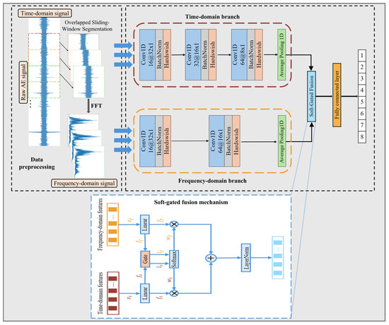
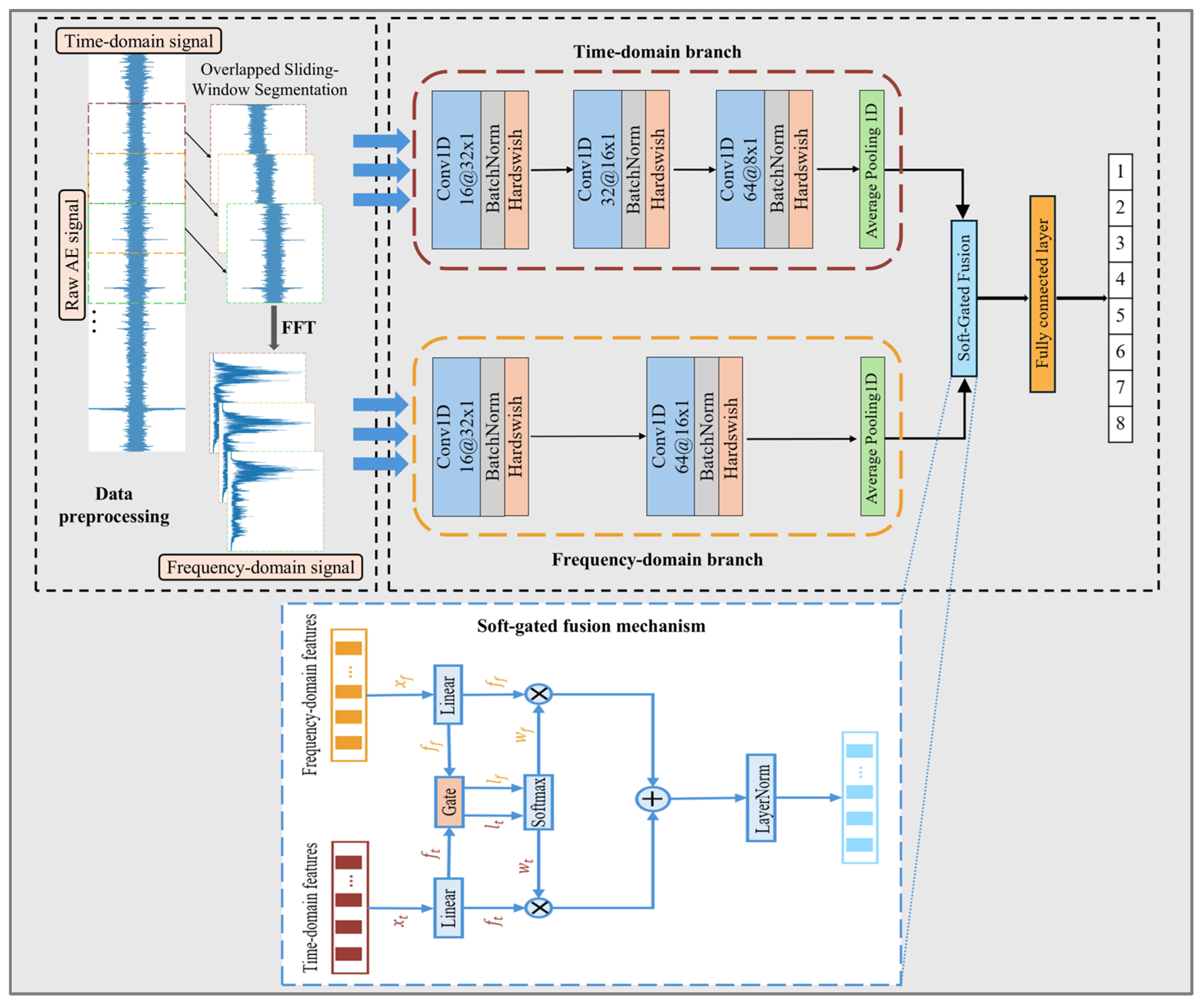
This study introduces the dual-stream network with the soft-gated fusion mechanism, termed DSGF-Net, to realize an efficient bearing fault diagnosis system (as illustrated in Figure 1). The proposed method comprises three primary stages. First, in the data preprocessing stage, raw AE signals are segmented using an overlapping sliding window technique to generate time-domain segments. Subsequently, the FFT is applied to each segment to obtain its corresponding frequency-domain spectral representation. The second stage is the parallel feature extraction stage: two distinct network branches (time- and frequency-domain branches) are optimized to learn domain-specific features. Each branch consists of stacked blocks structured as the 1D convolution—batch normalization—hard Swish activation function. The hard Swish activation function [35] is an optimized variant of the Swish activation function that offers superior computational efficiency and accuracy compared to traditional activation functions, such as the rectified linear unit (ReLU) or the original Swish function. Following the convolutional layers, a 1D average pooling layer is applied to compress the feature maps into compact embedding vectors. Finally, in the adaptive fusion stage, the soft-gated fusion mechanism synthesizes information from these two embedding vectors. A gate module receives features from both branches, computes logits, and applies the softmax function to generate dynamic weights (w_t and w_f). The two feature streams are then fused according to these weights and passed through layer normalization to stabilize the output distribution. The final fused feature vector is fed into a fully connected layer for fault classification. This architecture effectively exploits the complementarity between the time and frequency domains; the soft-gated mechanism automatically balances the contribution of each branch, thereby improving the accuracy of the proposed method while achieving low total latency.

3.2. Data Preprocessing

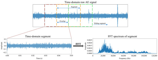
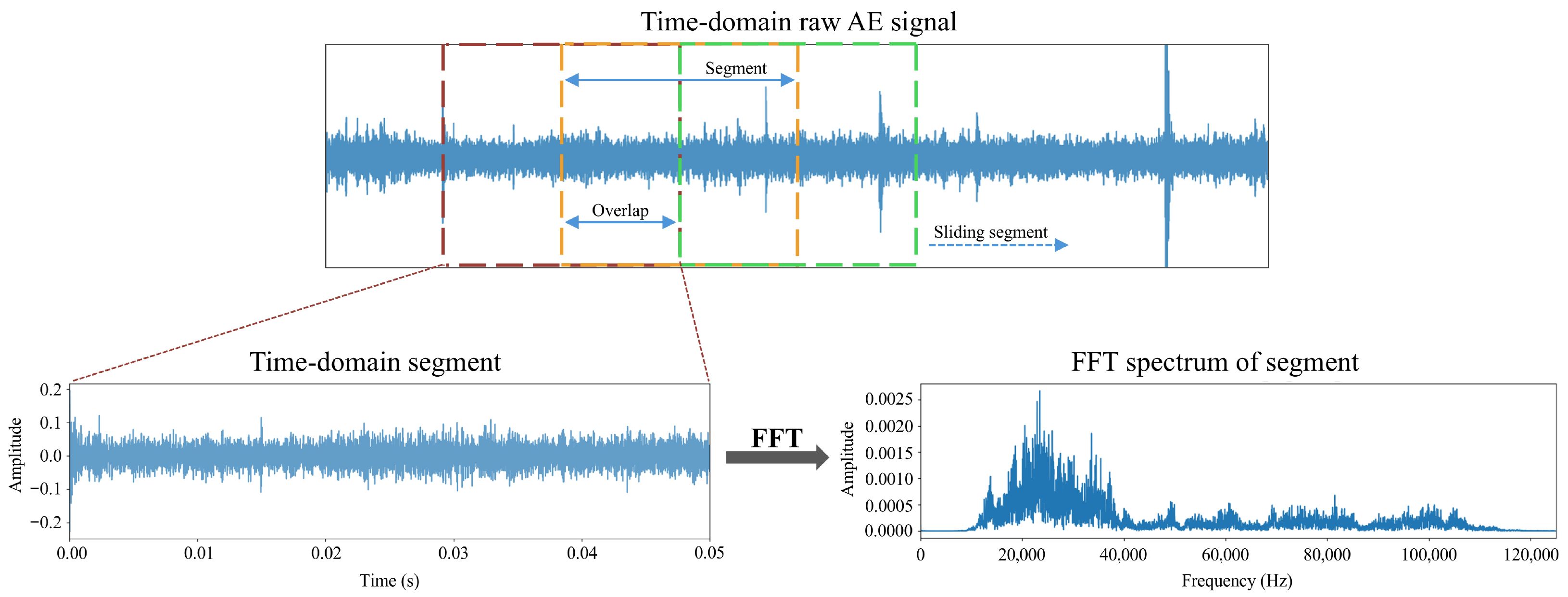
The initial step in the processing pipeline involves segmenting the raw time-domain signals into short overlapping segments, each with a duration of 0.05 s. This procedure not only augments the training dataset but also ensures data continuity (as illustrated in Figure 2). Subsequently, each time-domain segment is transformed into its frequency spectral representation using the FFT.

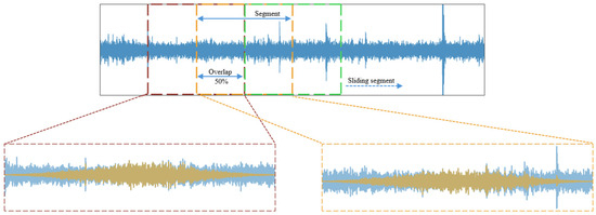
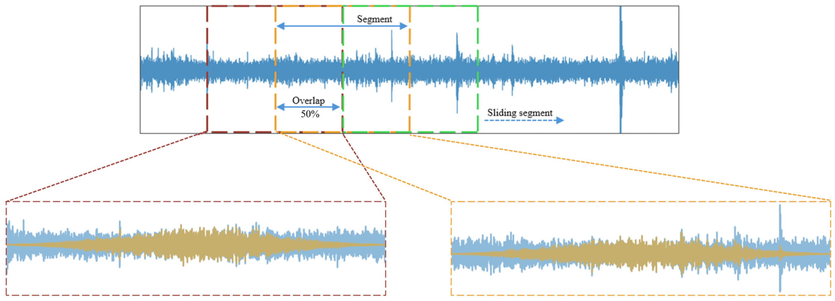
The selection of an appropriate window function is crucial for the FFT process. Although various common window functions exist, such as the Hamming and Blackman functions, this study employs the Hann window. For AE signals, the Hann window offers an optimal balance between maintaining frequency resolution and suppressing spectral leakage. However, local information loss may occur owing to the bell-shaped characteristics of the Hann window, thereby attenuating the signal amplitude to zero at both boundaries. To mitigate this issue, we apply an overlap ratio of 50% (as depicted in Figure 3, where the yellow envelope represents the Hann window application). This overlap ensures that information attenuated at the edges of the preceding segment is recovered by the central region of the subsequent segment, thereby preserving the integrity of the signal features.

Mathematically, the N-point DFT of the time-domain signal x[n] is defined as follows:

$${\mathrm{X}}^{\left(\mathrm{N}\right)}\left(\mathrm{p}\right) =\sum _{\mathrm{n} = 0}^{\mathrm{N}-1}\mathrm{x}\left[\mathrm{n}\right]{\mathrm{e}}^{-\mathrm{i}2\mathsf{\pi }\mathrm{pn}/\mathrm{N}}$$

(1)

where p = 0, 1, 2, …, N − 1; N denotes the number of DFT points and p is the discrete frequency index. In practice, the DFT is efficiently computed using the FFT based on a divide-and-conquer principle. For radix-2 decomposition, the DFT can be separated into even- and odd-indexed components as follows:

$${\mathrm{X}}^{\left(\mathrm{N}\right)}\left(\mathrm{p}\right)= \sum _{\mathrm{g} = 0}^{\mathrm{N}/2-1}\mathrm{x} \left[2\mathrm{g}\right]{\mathrm{e}}^{-\mathrm{i}2\mathsf{\pi }\mathrm{pg}/\mathrm{N}}+ {\mathrm{e}}^{-\mathrm{i}2\mathsf{\pi }\mathrm{p}/\mathrm{N}}\sum _{\mathrm{h} = 0}^{\mathrm{N}/2-1}\mathrm{x} [2\mathrm{h}+1]{\mathrm{e}}^{-\mathrm{i}2\mathsf{\pi }\mathrm{ph}/(\mathrm{N}/2)}$$

(2)

where g, h = 0, 1, 2, …, ${\displaystyle \frac{\mathrm{N}}{2}}$ − 1. From Equation (2), we can write this more compactly as follows:

$${\mathrm{X}}^{\left(\mathrm{N}\right)}\left(\mathrm{p}\right) = {\mathrm{X}}_0^{\left(\mathrm{N}/2\right)}\left(\mathrm{p}\right) + {\mathrm{e}}^{-\mathrm{i}2\mathsf{\pi }\mathrm{p}/\mathrm{N}}{\mathrm{X}}_1^{\left(\mathrm{N}/2\right)}\left(\mathrm{p}\right)$$

(3)

Because the input AE signals are real-valued, the resulting spectrum exhibits conjugate symmetry. Consequently, to optimize memory usage and reduce computational cost, this study utilizes only a single-sided spectrum (positive-frequency components). Specifically, with a sampling rate of 250 kHz, each raw AE signal is divided into 0.05 s segments, yielding 12,500 samples per segment. This duration of each segment provides a frequency resolution of approximately 20 Hz, which helps separate closely spaced fault-related spectral components.

Following the real FFT operation, the resulting frequency-domain feature vector has a length of N/2 = 6250 points, representing the frequency range of 0–125 kHz (as shown in Figure 2). However, feeding such high-resolution input (6250 points) directly into the 1D CNN would impose significant computational cost. Therefore, rather than sacrificing spectral resolution by shortening the time window, we adopt a strategy of resampling the magnitude spectrum to a fixed lower size (e.g., 4096, 2048, or 1024 points) before feeding it into the model. This approach optimally balances diagnostic accuracy and computational efficiency.

3.3. Dual-Stream Feature Extraction Network

3.3.1. Temporal Feature Extraction Branch

The time-domain branch is designed to capture temporal dependencies and impulsive patterns directly from raw segmented AE signals, each having length of 12,500 points. As illustrated in the upper part of Figure 1, this branch is constructed by stacking three consecutive convolutional blocks, followed by an average pooling layer. Each block comprises a 1D convolutional layer, a batch normalization layer to accelerate convergence, and a hard swish activation function to introduce nonlinearity at low computational cost, as shown in Equation (4):

$$\mathrm{Hardswish}\left(\mathrm{x}\right) = \mathrm{x}·{\displaystyle \frac{\mathrm{ReLU}6\left(\mathrm{x} + 3\right)}{6}}$$

(4)

where x is the input value and ReLU6 is the Rectified Linear Unit 6 function, which outputs u if u is between zero and six, zero if u is negative, and six if u is greater than six.

This study adopts a multi-scale kernel strategy, in which the kernel size decreases progressively through the layers (32 × 1 → 16 × 1 → 8 × 1). The large kernel in the first layer provides a wide temporal receptive field, enabling the model to capture long-term temporal components and shape extended pulse patterns, while the smaller kernels in subsequent layers extract more detailed and abstract features. The number of filters increases (16 to 32 to 64) to enrich the temporal feature representation. Finally, the 1D average pooling layer compresses the feature maps along the time axis into a compact embedding vector that serves as the input for the fusion mechanism.

3.3.2. Spectral Feature Extraction Branch

Alongside the time-domain branch, the spectral feature extraction branch processes the input using the spectral magnitude obtained from the FFT stage. Because the frequency-domain input is shorter in length than the time-domain sequence, a shallow network architecture is sufficient to effectively extract classification features while also reducing the model weight and parameter count.

As shown in Figure 1, this branch consists of two convolutional blocks. Similar to the time-domain branch, each block integrates 1D convolution, batch normalization, and the hard swish activation function. The first layer uses the kernel size of 32 × 1 with 16 filters to extract broad spectral patterns, whereas the second layer uses the 16 × 1 kernel with 64 filters to learn fault-specific spectral signatures. By processing data directly in the frequency domain, this branch reduces the sensitivity to temporal shifts of the input signal and easily identifies characteristic fault frequencies, which appear as prominent peaks in the spectrum. The extracted spectral features are also flattened using the average pooling layer before being fed into the fusion stage.

3.4. Soft-Gated Fusion Mechanism

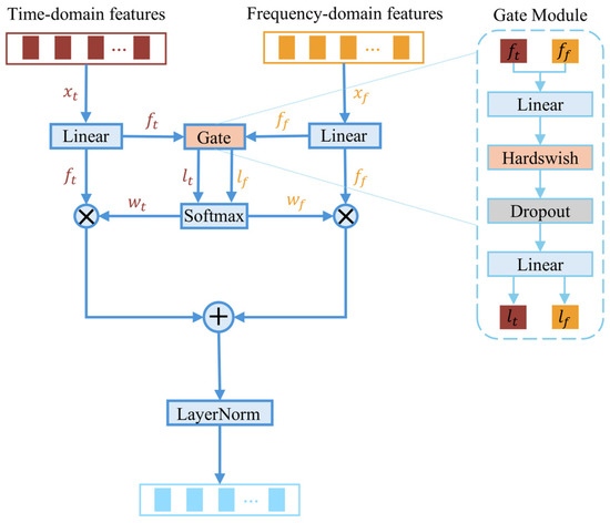
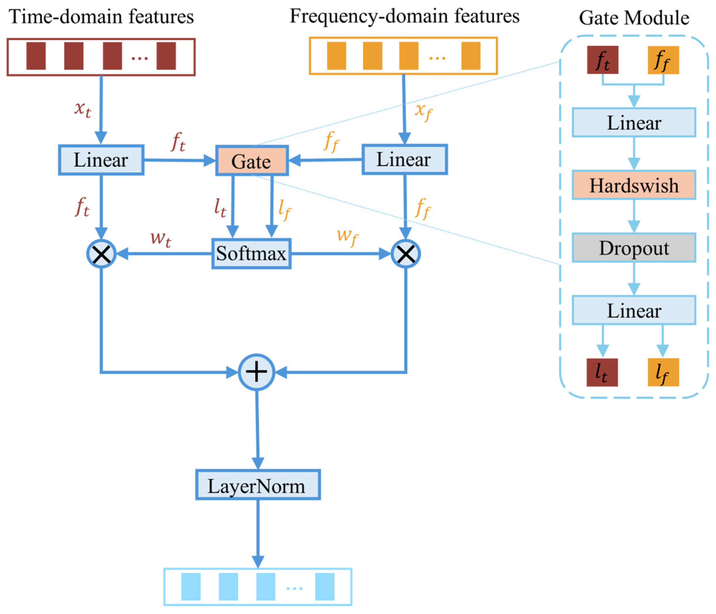
The soft-gated fusion mechanism is an adaptive feature fusion method in which the model learns to allocate the contributions of the time and frequency domains according to the context of each sample, rather than using a fixed mixture (as depicted in Figure 4). This approach improves reliability when one branch is less informative, while maintaining a low computational cost and training stability.

Structurally, each branch provides a feature vector projected onto a common dimension. A lightweight gate module then processes these representations to estimate soft weights using the softmax function, reflecting the relative reliability of each branch, as expressed by Equations (5) and (6):

$${\mathrm{w}}_{\mathrm{t}} = {\displaystyle \frac{{\mathrm{e}}^{{\mathrm{l}}_{\mathrm{t}}}}{{\mathrm{e}}^{{\mathrm{l}}_{\mathrm{t}}}+ {\mathrm{e}}^{{\mathrm{l}}_{\mathrm{f}}}}}, {\mathrm{w}}_{\mathrm{f} }= {\displaystyle \frac{{\mathrm{e}}^{{\mathrm{l}}_{\mathrm{f}}}}{{\mathrm{e}}^{{\mathrm{l}}_{\mathrm{t}}}+ {\mathrm{e}}^{{\mathrm{l}}_{\mathrm{f}}}}}, {\mathrm{w}}_{\mathrm{t}}+ {\mathrm{w}}_{\mathrm{f}} = 1$$

(5)

$${\mathbf{F}}_{\mathrm{fusion}} ={\mathrm{w}}_{\mathrm{t}}{·\mathrm{x}}_{\mathrm{t}} +{\mathrm{w}}_{\mathrm{f}}·{\mathrm{x}}_{\mathrm{f}}$$

(6)

where x_t and x_f are two feature vectors after projection, and l_t and l_f are two logits from the gate module. Subsequently, the module produces a fused feature by emphasizing the more useful branch while attenuating the less informative one (as shown in Equation (6)). Through this soft fusion scheme, the model remains differentiable and stable, while helping to prevent a single branch from dominating. Next, layer normalization after fusion helps smooth the dominant temporal pulse cues when dynamic information is key or preserves characteristic spectral patterns when frequency-domain features are more informative. Moreover, the mechanism is parameter efficient and can be easily integrated into various architectures. Ultimately, it yields a fused representation that is robust, stable, and informative, enhancing system reliability when operating conditions change or when either branch is contaminated by noise.

4. Experiments and Results

4.1. Experimental Methods

4.1.1. Experimental System and Dataset

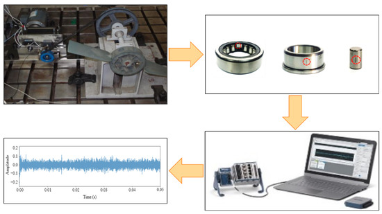
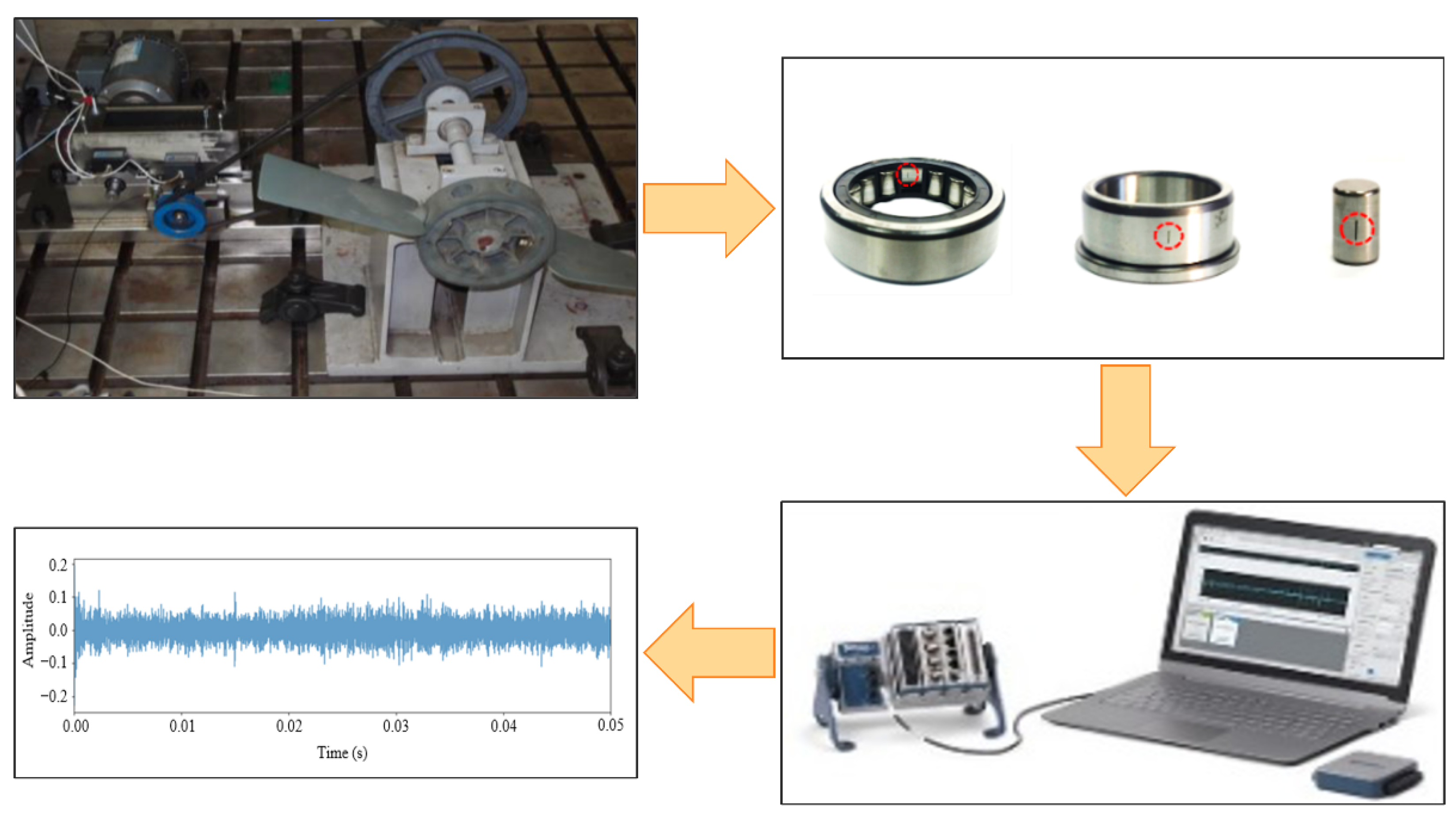
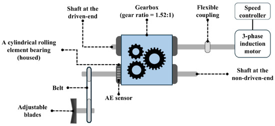
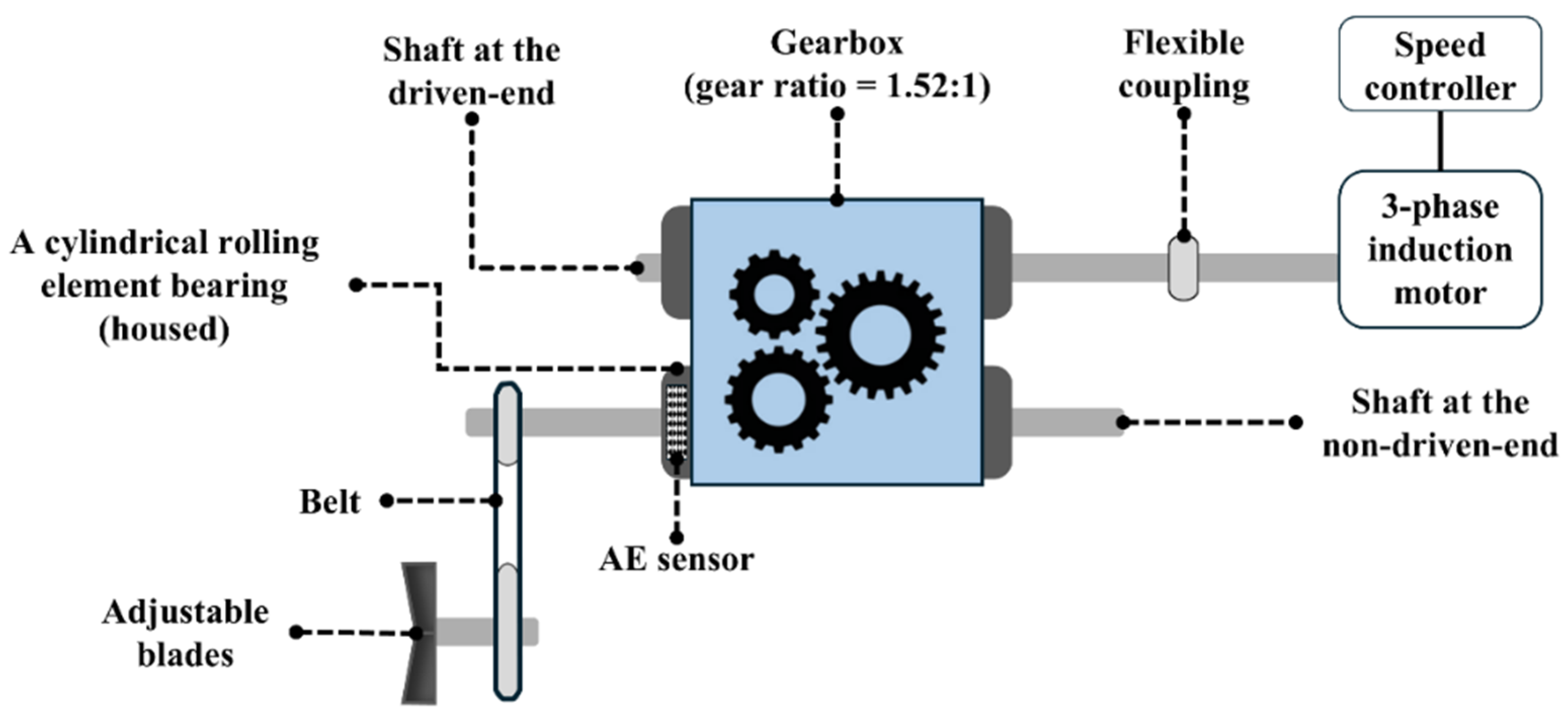
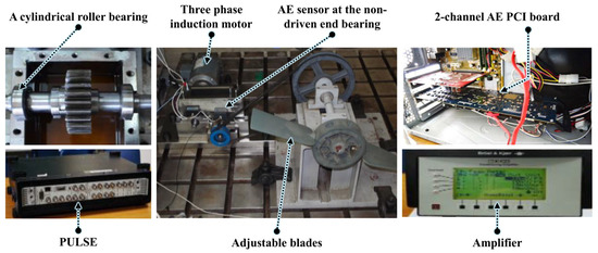
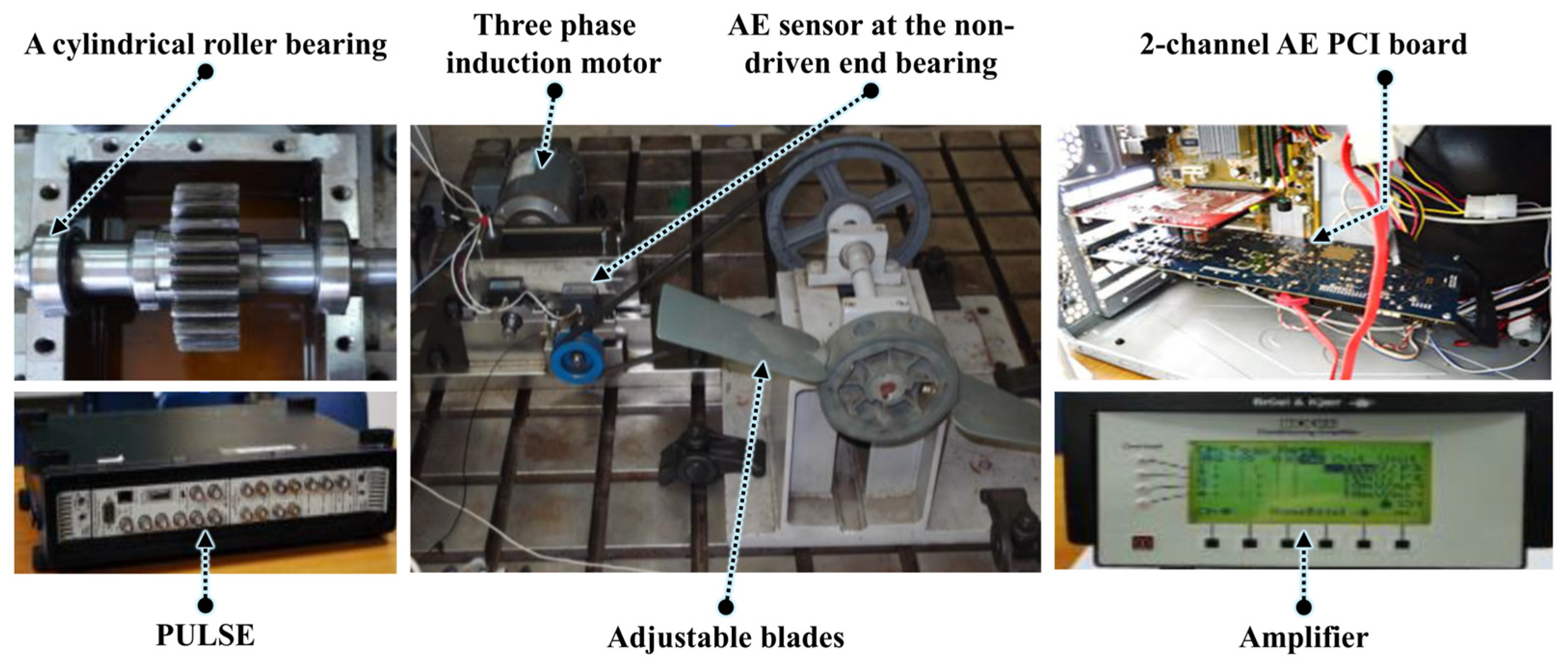
An experimental system used to collect data for BFD has been widely used in previous studies [36,37]. For clarity, Figure 5 provides an overview of the bearing AE acquisition workflow. The AE signals are collected during the experiments and stored as raw time-series recordings. These recordings are stored and transferred to MATLAB (R2024b), where they are arranged and prepared for the subsequent analysis steps. In terms of the mechanical setup, the system includes a 3-phase induction motor that allows speed variation using a speed controller. In addition, the driven-end and non-driven-end shafts are connected through a gearbox with a gear ratio of 1.52:1 (as illustrated in Figure 6 and Figure 7). These shafts are mounted onto a test bench and attached to a cylindrical roller bearing (FAG NJ206-E-TVP2). Figure 6 shows the non-driven-end shaft connected to an adjustable blade via a belt and pulley, serving as a variable load for the system. A flexible coupling connects the motor shaft to the driven-end shaft, thereby helping to prevent shock transmission.

In the data acquisition system, a wideband AE sensor (PAC WSα) is mounted on the bearing housing adjacent to the non-driven-end target bearing to ensure that the acquired signals predominantly reflect the condition of the target bearing rather than the opposite bearing. The effective frequency range of the AE sensor is from 100 to 900 kHz, the range of the frequency response is from 1 kHz to 3 MHz, the peak sensitivity is −62 dB; ±1.5 dB directionally, and the resonant frequency is 650 kHz. In this study, the recorded AE signals were used for classification-model development rather than for broadband ultrasonic characterization of the sensor. AE signals were acquired from the sensor using a PCI-2-based board and analyzed at a decimated sampling rate of 250 kHz. This decimation was performed in MATLAB using the built-in decimate() function with a decimation factor of 4, which applies a low-pass filter to suppress out-of-band components and prevent aliasing. With a decimated sampling rate of 250 kHz, the corresponding Nyquist frequency is 125 kHz, and thus the usable one-sided spectrum of the recorded signal is limited to 0–125 kHz. This acquisition setting has also been adopted in prior bearing fault diagnosis studies using the same experimental system [1,36,37,38], supporting its practical suitability for classification-oriented analysis. The detailed specifications of the experimental bearings and fault characteristics frequencies (FCFs) are listed in

Table 1. Detailed specifications of the experimental setup and fault characteristics frequencies.

Number of rolling elements	13
Contact angle	0°
Pitch diameter	46.5 (mm)
Rolling element diameter	9.0 (mm)
Roller defect frequency	2.487 × 2 × fr
Outer defect frequency	5.241 × fr
Inner defect frequency	7.758 × fr

.

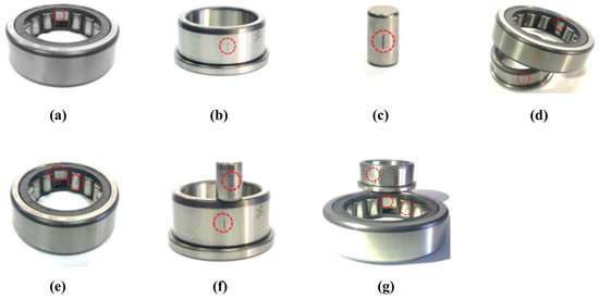
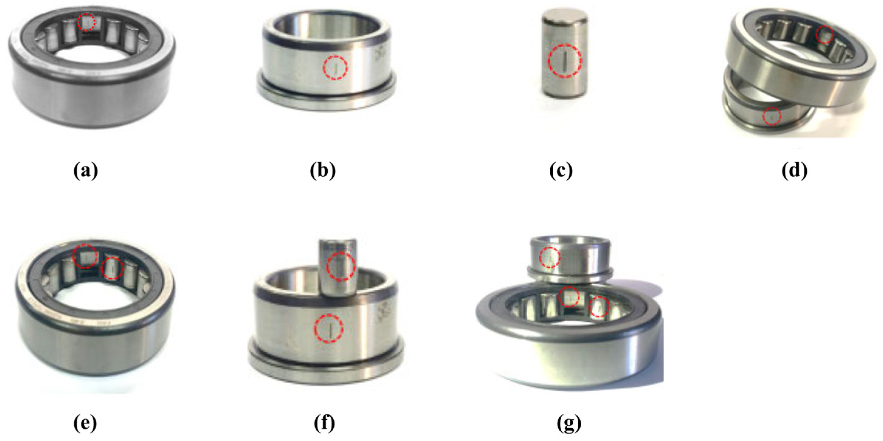
We fabricated various bearing fault types with varying sizes and locations on a single physical bearing specimen using a diamond cutting method at different location on bearing (illustrated in Figure 8). This resulted in a dataset with three crack sizes (3, 6, and 12 mm), seven classes comprising single and compound faults as well as one normal condition. For each condition, the original AE recordings were acquired as 1 s signals and then divided into 0.05 s segments. The segment duration was selected to ensure that each segment contained sufficient fault-relative information while keeping the acquisition time as short as possible. To determine an appropriate segment duration, the FCFs were estimated using empirical formulas based on the bearing geometry and shaft rotational speeds [38]. Because these frequencies are linearly related to the rotational speed, the lowest FCF in the operating speed range was used as the main reference. In this way, the selected segment length was long enough to include representative fault-relative periodic components even under the lowest-speed condition. Based on this analysis and repeated preliminary experiments, 0.05 s was finally adopted as the segment duration.

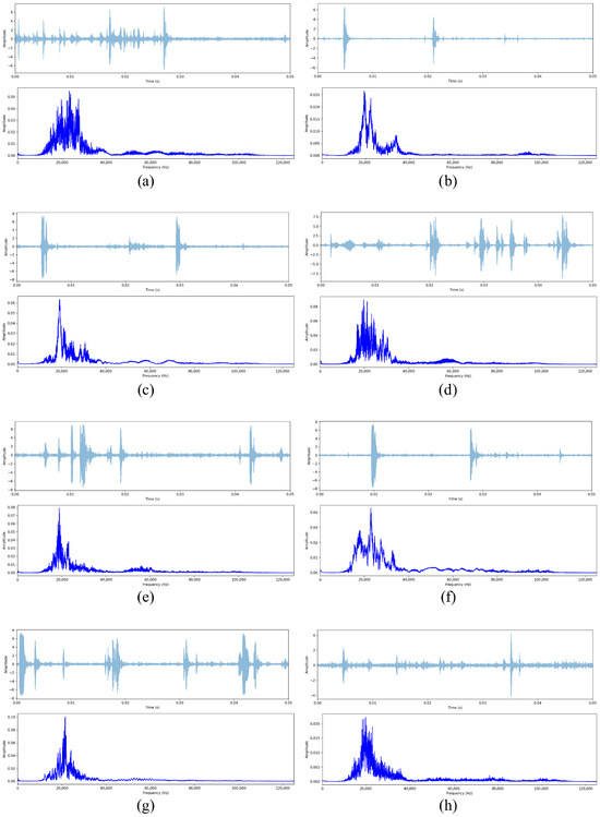
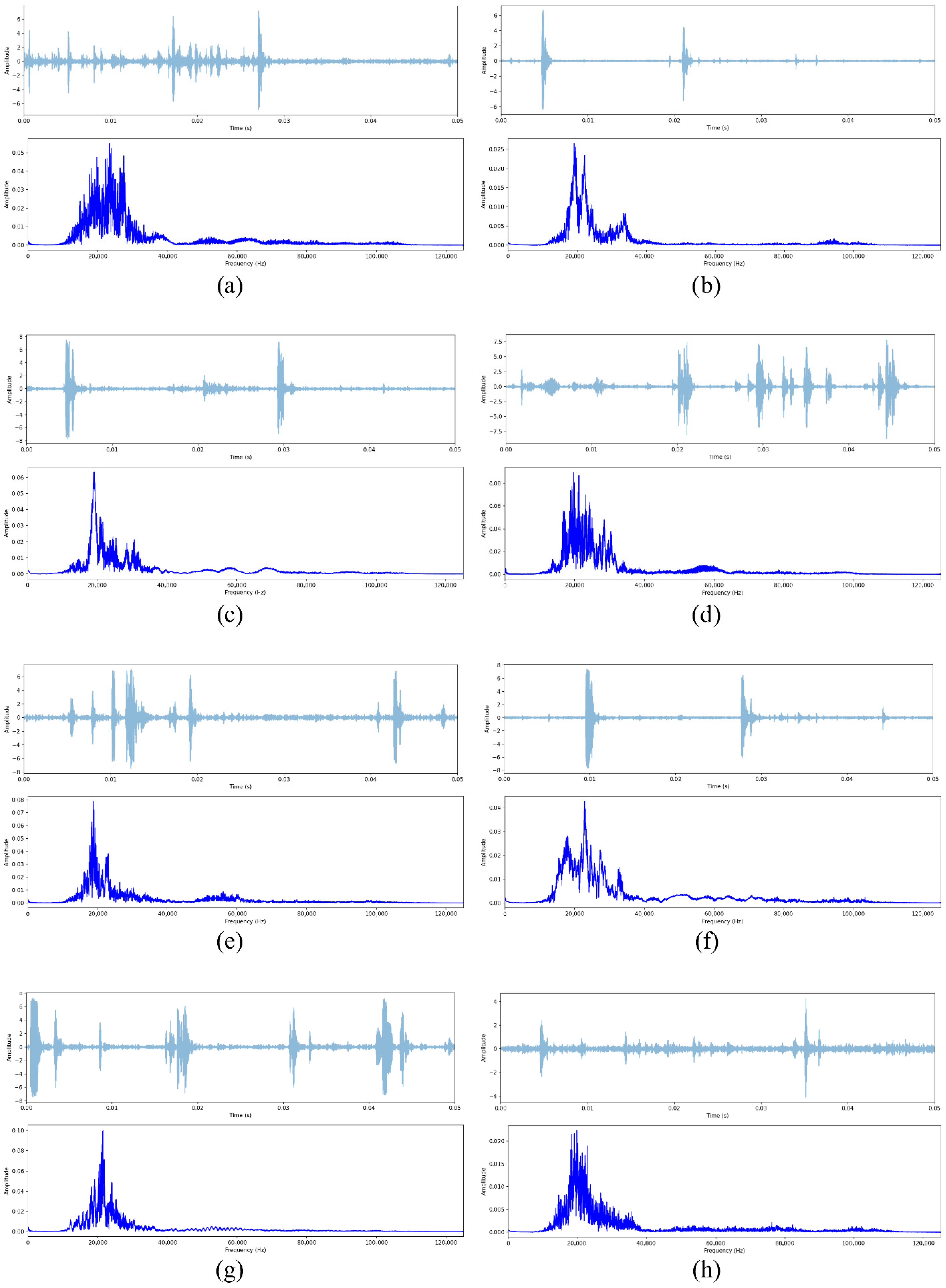
The original datasets were independently separated into training, validation, and testing subsets before segmentation. Specifically, signals collected at 300, 400, and 500 rpm were used for training subset, whereas the validation and testing subsets were derived from signals recorded at 250, 350, and 450 rpm. After partitioning, we confirmed that no duplicated segments were shared among the training, validation, and testing subsets. The partitioning details are presented in

Table 2. Details of the proposed bearing fault diagnosis dataset.

Subset	Crack Size			Speed (RPM)	No. of Classes	Temporal Samples	Spectral Samples
	Length (mm)	Width (mm)	Depth (mm)
Training	3	0.6	0.3	300, 400, 500	8	4800	4800
	6	0.6	0.5
	12	0.6	0.5
Validation	3	0.6	0.3	250, 350, 450	8	1200	1200
	6	0.6	0.5
	12	0.6	0.5
Testing	3	0.6	0.3	250, 350, 450	8	2400	2400
	6	0.6	0.5
	12	0.6	0.5

. During model development, only the training and validation subsets were employed, and the testing subset remained untouched until the final assessment of the proposed method’s overall performance. Figure 9 displays representative time-domain signals and their FFT magnitude spectra for eight bearing health conditions (one healthy and seven faulty). In each subpanel, the upper plot shows the time-domain waveform, while the lower dark-blue curve shows the FFT magnitude spectrum, enabling quick visual comparison across conditions.

4.1.2. Network Parameters

As presented in the previous sections, each convolutional block of both branches follows the order conv1D → batch normalization → hard swish, without using padding, and employs a fixed stride of four; this approach ensures a genuine, layer-by-layer reduction in feature length and mitigates boundary artifacts. After the convolutional sequence, each branch applies 1D adaptive average pooling to aggregate the features into a single position and then compresses them into the compact vector. Finally, a dropout rate of 0.3 is used to reduce overfitting and improve the model’s robustness to noise. The detailed parameters are provided in

Table 3. Description of the proposed architecture.

Frequency-Domain Branch					Time-Domain Branch
Type	In/Out Channel	Kernel Size	Stride	Padding	Type	In/Out Channel	Kernel Size	Stride	Padding
Conv1D	1/16	32	4	0	Conv1D	1/16	32	4	0
Conv1D	16/64	16	4	0	Conv1D	16/32	16	4	0
Adaptive AvgPool1D	64/1	1	-	-	Conv1D	32/64	8	4	0
Dropout	-	-	-	-	Adaptive AvgPool1D	64/1	1	-	-
					Dropout	-	-	-	-
Soft-gated fusion
Type			Input channel			Output channel
Linear (Time feature)			64 × 1			64 × 1
Linear (Frequency feature)			64 × 1			64 × 1
Gate module			128 × 1			2 × 1
Softmax & weighted Sum			2 × 1 & 64 × 1			64 × 1
LayerNorm			64 × 1			64 × 1
Fully connected layer
BatchNorm			64 × 1			64 × 1
Hardswish			-			-
Linear			64 × 1			8 × 1

.

In the fusion stage, the two feature vectors from the branches are projected into the common space (64 × 1), concatenated, and passed through the gating module to produce sample-adaptive soft weights. The fused representation is then formed as a weighted linear combination of the two vectors, followed by layer normalization to stabilize the distribution. The final classifier uses the sequence of batch normalization → hard swish → linear to map the features to the target fault classes. This design yields an architecture that is robust, provides reproducible results, and resists domination by any single branch.

The model was trained using the AdamW optimizer (learning rate 0.001, weight decay 0.0005) and a batch size of 32. To balance fast early processing with stable convergence, we applied a learning-rate scheduler that gradually adjusted the learning rate over time. Cross-entropy was used as the loss function, and the network was trained for 30 epochs. All development and evaluation of the model were conducted using the PyTorch framework (version 2.8.0), utilizing an Intel i7 14700 28-core CPU and an NVIDIA GeForce RTX 5060 16 GB GPU.

4.2. Experimental Results and Discussion

4.2.1. Performance Evaluation of Different FFT Lengths

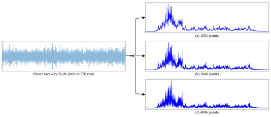
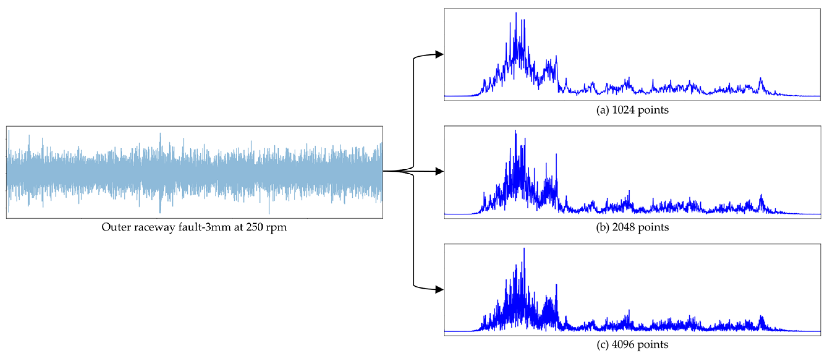
The frequency-spectrum resolution directly affects diagnostic accuracy and can be adjusted by changing the number of FFT points. Selecting an appropriate FFT length (NFFT) is essential to build a lightweight model while maintaining a good diagnostic accuracy. In this study, we standardized and visually compared three numbers of NFFT points: 1024, 2048, and 4096. For real signals such as AE signals, the frequency spectrum after the FFT is symmetric around 0 Hz. Therefore, to reduce the memory footprint, we retained only the positive (one-sided) frequency spectrum. In the input data, 12,500 NFFT points were used, corresponding to 6250 points representing the one-sided frequency spectrum. Figure 10a–c illustrate the frequency spectra of an outer raceway at crack size of 3 mm and rotational speed of 250 rpm after resampling to the three NFFT point counts mentioned above. All plots are displayed on the same frequency axis scale to ensure a fair visual comparison.

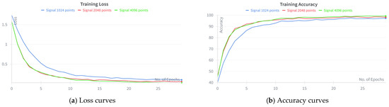
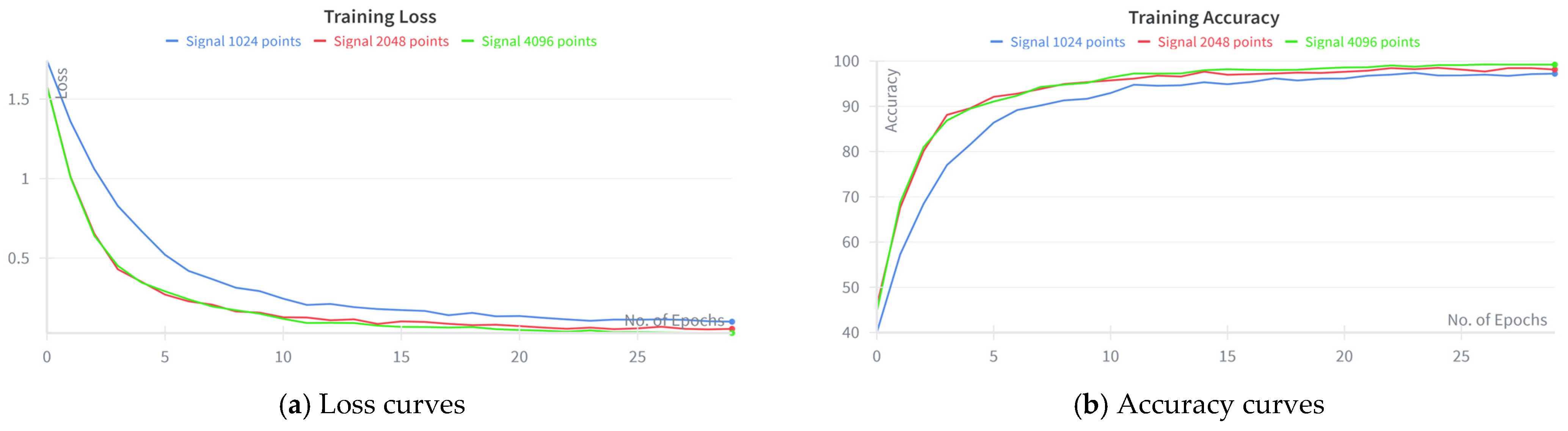
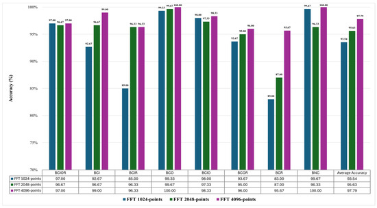
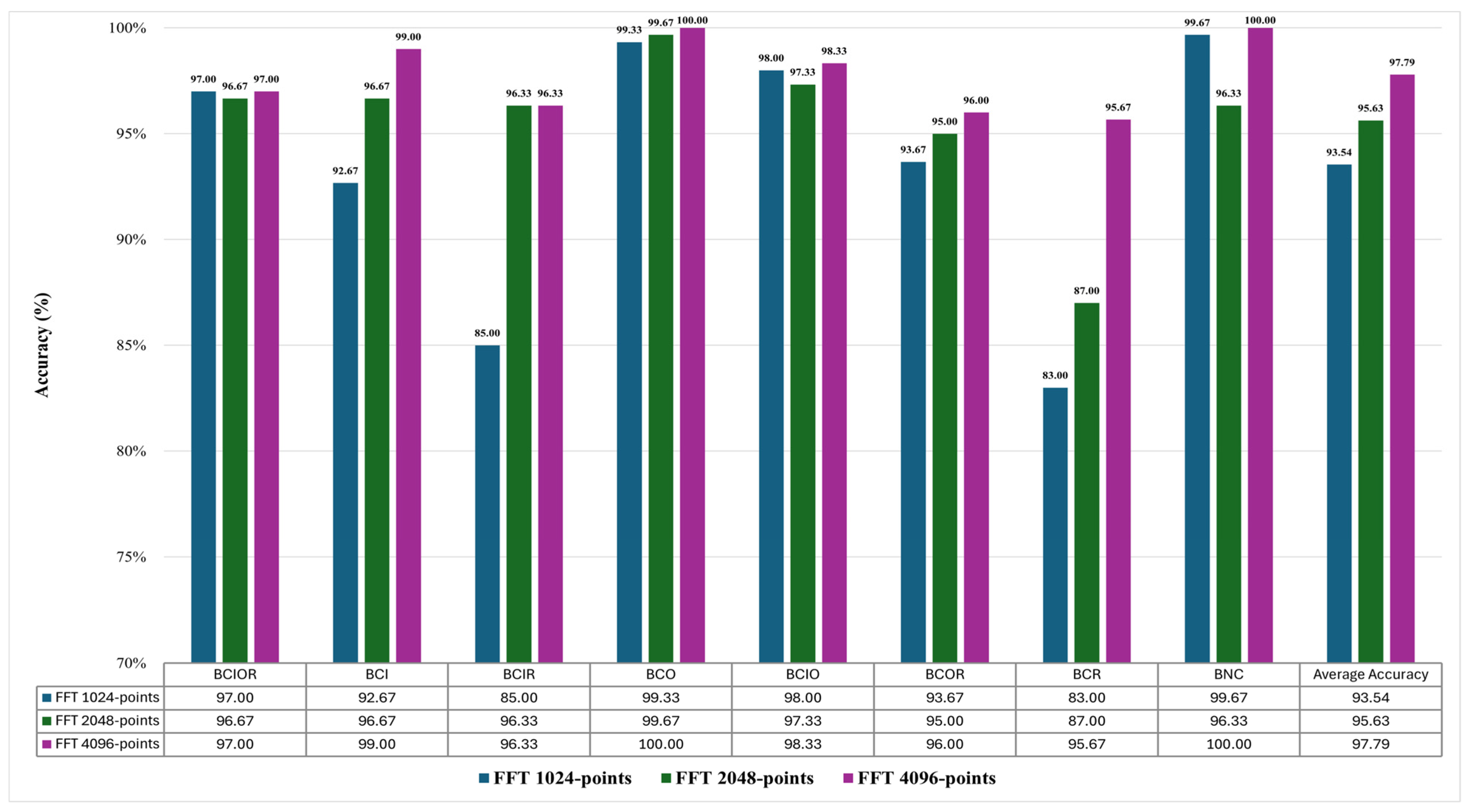
Increasing the number of FFT points enriches the spectral information, enabling the model to learn frequency features more precisely and distinguish adjacent peaks more effectively, thereby improving optimization speed and training accuracy. Figure 11 displays the loss and accuracy curves during the training stage, whereas Figure 12 illustrates the impact of different FFT lengths on diagnosis accuracy across eight fault types (BCIOR, BCI, BCIR, BCO, BCIO, BCOR, BCR, and BNC) and the overall average. The results show that performance generally improves as the number of NFFT points increases from 1024 to 2048 and then to 4096. Therefore, we chose to use 4096 NFFT points, achieving a reduction of roughly 1.5 times compared to the original number of points (6250), while achieving good diagnostic accuracy, reducing the memory footprint, and saving computational resources.

4.2.2. Performance of the Proposed Method

All data in the training, validation, and testing subsets were transformed using the FFT to obtain frequency-spectrum representations. To assess the effectiveness of the signal preprocessing strategy, we measured the processing times of the FFT and STFT. Our objective was to clarify the computational advantages of the proposed method at each stage of the bearing fault diagnosis pipeline compared with approaches that use 2D time–frequency image inputs. Nguyen and Kim [1] showed that for the same AE signal segment, the STFT is computationally more efficient and faster than the CQT and HHT techniques. Therefore, in this study, we compared only the FFT and STFT using the same window function and number of FFT points.

Table 4. Processing time of STFT and FFT techniques measured.

Processing Method	Average Processing Time of One Signal (ms)	Average Processing Time of One Segmented Signal (ms)
STFT	602.162	30.108
FFT	21.995	0.564

shows that the FFT requires only 21.995 ms to process a full-length signal, being nearly 27 times faster than the STFT, and takes only 0.564 ms per segmented signal, which is approximately 53 times faster. These results reinforce the idea that the proposed method is well suited to resource-constrained environments, thereby opening a promising avenue for real-time bearing fault diagnosis.

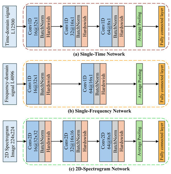
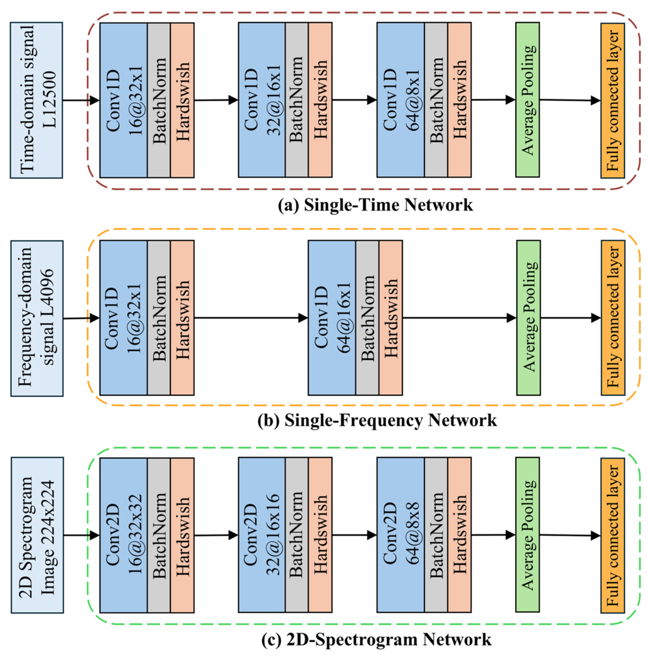
To validate the effectiveness of the proposed method, comparative experiments were conducted using several baseline and reference architectures under a unified training and evaluation protocol, as illustrated in Figure 13. Single-Time Network (ST-Net) is a 1D CNN model that is implemented based on the time-domain branch and uses time-domain signals as the input. Single-Frequency Network (SF-Net) is 1D CNN model based on the frequency-domain branch, with frequency spectrum signals as the input. 2D-Spectrogram Network (2D-SpecNet) is 2D CNN model, which is configured similarly to ST-Net but uses 2D convolutional layers and 2D average pooling, and receives 2D time–frequency images of size 224 × 224 as input. In addition, two fusion-based ablation variants were included: DSGF-Net (Concatenation), in which the time- and frequency-domain features are directly concatenated before classification, and DSGF-Net (Fixed-weight, w_t:w_f = 0.5:0.5), which fuses the two branches using an equal fixed weighting ratio. To further broaden the comparison, the fusion-based model (TD-MDA) in [29] was also re-implemented under the same input setting as the proposed method, while preserving its original architectural design as closely as possible and applying the same general experimental configuration. For all compared models, the final fully connected layer was used for BFD.

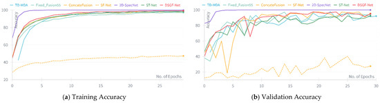
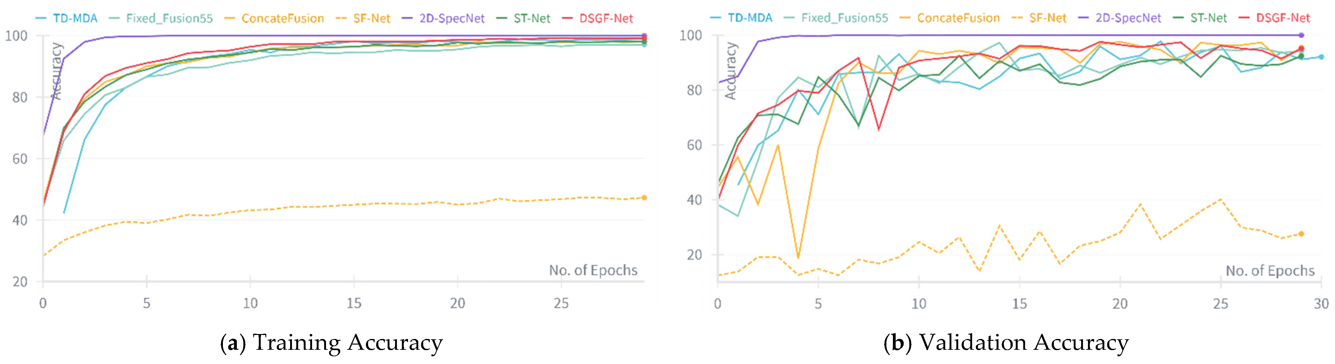
Figure 14a shows the training accuracy curves of the compared methods. DSGF-Net accelerated strongly from the first epochs and quickly reached high accuracy; compared with 2D-SpecNet, DSGF-Net was only slightly slower in initial convergence, but it maintained smooth, stable operation and outperformed other methods, while being considerably superior to SF-Net. Figure 14b shows the validation accuracy curves. On the validation subset, the proposed method sustained high accuracy; although localized fluctuations were observed in the middle epochs, the model recovered quickly in later epochs and closely tracked the nearly saturated curve of 2D-SpecNet. The consistency between the two plots indicates that DSGF-Net achieved an optimal balance among convergence speed, asymptotic accuracy, and stability, while outperforming other methods and significantly surpassing SF-Net throughout both training and validation.

As shown in

Table 5. Comparative best-performing results of different methods with the same architecture. The best value of the proposed model corresponds to highest obtained across repeated experiments.

Model	Data Input	MACs (M)	Params (M)	Inference Latency (ms)	Throughput (Batches/s)	Best Accuracy (%)
DSGF-Net (Soft-Gated Fusion)	Time- and frequency-domain signals	16.2576	0.04540	1.39	716.93	97.79
ST-Net	Time-domain signals	11.4769	0.02607	0.86	1159.83	92.04
SF-Net	Frequency-spectrum signals	4.7793	0.01778	0.65	1527.54	41.21
2D-SpecNet	2D time–frequency images	128.8042	0.31251	0.84	1191.73	99.95
DSGF-Net (Concatenation)	Time- and frequency-domain signals	16.2573	0.04503	1.00	996.00	97.08
DSGF-Net (Fixed-weight wt:wf = 0.5:0.5)	Time- and frequency-domain signals	16.2571	0.04484	1.13	884.86	96.92
TF-MDA [29]	Time- and frequency-domain signals	7.2617	0.03798	1.99	502.27	97.00

, DSGF-Net achieved a balanced trade-off between classification performance and model complexity. Compared with 2D-SpecNet, DSGF-Net markedly reduced the computational cost, using only 16.2576 M MACs and 0.0454 M parameters, corresponding to reductions of 87.4% in MACs and 85.5% in parameter count, whereas its best accuracy was lower by only 2.16 percentage points (97.79% vs. 99.95%). Compared with single-domain baselines ST-Net and SF-Net, DSGF-Net consumed more resources (MACs 41.7% higher than that of ST-Net and 3.4 times higher than that of SF-Net; parameter count 74.6% higher than that of ST-Net and 2.55 times than that of SF-Net). However, it achieved substantially better accuracy, improving by 5.75 percentage points over ST-Net (92.04%) and 56.58 percentage points over SF-Net (41.21%).

Among the fusion-based variants, DSGF-Net with soft-gated fusion mechanism consistently achieved the highest best accuracy. Specifically, it outperformed DSGF-Net with simple concatenation by 0.71 percentage points (97.79% vs. 97.08%) and DSGF-Net with fixed-weight fusion by 0.87 percentage points (97.79% vs. 96.92%). Notably, these three variants had almost identical MACs and parameter counts, indicating that the performance improvement mainly came from the soft-gated fusion mechanism rather than from increased model size or computational cost.

In comparison TF-MDA [29], DSGF-Net also achieved higher best accuracy improvement of 0.79 percentage points (97.79% vs. 97.00%). Although DSGF-Net required more MACs (16.2576 M vs. 7.2617 M) and parameters (0.0454 M vs. 0.03798 M), this result suggests that the proposed method provides a more effective use of dual-stream information for AE-based BFD.

In terms of inference speed, DSGF-Net showed lower throughput and higher latency than the most comparison models. Its throughput was 716.93 batches/s, which was lower than that of 2D-SpecNet (39.9%), ST-Net (38.2%), SF-Net (53.1%), the DSGF-Net variant with concatenation (28.0%), the DSGF-Net variant with fixed-weight fusion (19.0%), but still higher than method [29] (42.7%). Its inference latency was 1.39 ms, which was higher than 2D-SpecNet (0.84 ms), ST-Net (0.86 ms), SF-Net (0.65 ms), the concatenation variant (1.00 ms), and the fixed-weight fusion variant (1.13 ms), but lower than that of method [29] (1.99 ms). Overall, these results indicate that DSGF-Net does not provide the fastest inference, but it offers a reasonable balance between complexity and accuracy, while the soft-gated fusion yields consistent improvement over simpler fusion strategies.

To complement the best-result comparison in Table 5,

Table 6. Statistical comparison of the proposed method and comparison models over five runs.

Method	Accuracy (%) (Mean ± std)	Paired t-Test vs. Proposed Method
DSGF-Net (Soft-Gated Fusion)	97.45 ± 0.327	−
ST-Net	91.57 ± 0.551	8.58 × 10−6
SF-Net	40.62 ± 0.716	1.30 × 10−9
2D-SpecNet	99.89 ± 0.068	7.83 × 10−5
DSGF-Net (Concatenation)	96.17 ± 0.759	0.0181
DSGF-Net (Fixed-weight wt:wf = 0.5:0.5)	95.39 ± 0.881	0.00974
TF-MDA [29]	96.24 ± 0.473	0.001997

reports the statistical comparison results over five runs. The results are presented as mean ± standard deviation, and the last column provides p-values obtained from a two-sided paired t-test against DSGF-Net. Here, the p-value evaluates whether the run-wise performance difference between DSGF-Net and each comparison model is statistically significant rather than caused by random variation. Since all p-values are below 0.05, the results indicate that the performance differences between DSGF-Net and the compared models are statistically significant. These findings support that the advantage of DSGF-Net is not limited to a single best run but remains consistent across repeated experiments.

Considering the end-to-end latency (including signal processing and CNN inference time), DSGF-Net demonstrated computational efficiency superior to that of 2D-SpecNet. Specifically, DSGF-Net attained a total latency of 1.95 ms, representing a 93.7% reduction relative to the 30.95 ms of 2D-SpecNet, while preserving high diagnostic accuracy. Compared with other 1D CNN-based methods, DSGF-Net exhibited a higher total latency than ST-Net (0.86 ms) and SF-Net (1.21 ms); however, it consistently delivered superior diagnostic accuracy. As summarized in

Table 7. Latency comparison between the proposed method and other methods on the Intel Core i7-14700.

Method	Signal Processing Time (ms)	CNN Inference Time (ms)	Total Latency (ms)
DSGF-Net	0.564	1.39	1.954
ST-Net	-	0.86	0.86
SF-Net	0.564	0.65	1.214
2D-SpecNet	30.108	0.84	30.948

, these results confirm that DSGF-Net achieves a favorable balance between computational efficiency, latency, and diagnostic performance.

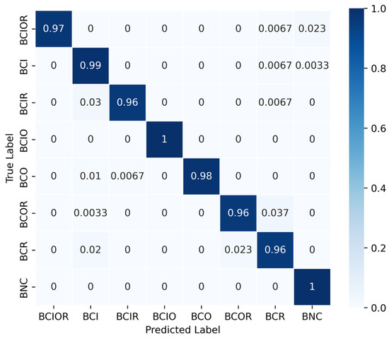
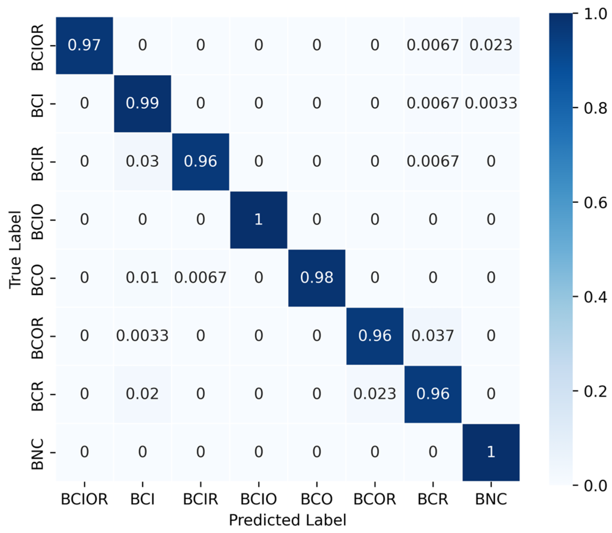
The confusion matrices in Figure 15 illustrate the classification results of the proposed method. Each row denotes a true class and each column represents a predicted class. The dark diagonal cells signify correct predictions, and all values along the diagonal indicate that most faults were identified with high class-wise sensitivity. In particular, BCIO and BNC achieved 100% sensitivity, whereas BCI showed nearly 100% sensitivity. The remaining misclassifications are minor and mainly concentrated within specific fault pairs that share closely related mechanical mechanisms: BCOR-BCR ≈ 3.7%, BCR-BCOR ≈ 2.3%, and BCIR-BCI ≈ 3.0%. This localized confusion arises primarily because these paired conditions share the same dominant fault frequencies (rolling element frequency for roller-related faults and inner race frequency for inner-race faults). Meanwhile, the sidebands associated with the secondary fault components can become blurred or obscured within a short segment (0.05 s) under low rotational speeds or small crack sizes, leading to off-diagonal misclassification rates of approximately 2–4%. Overall, the model achieved high accuracy across classes.

Table 8. Statistical analysis of the learned fusion weights across fault categories on the test set.

Fault Type	Number of Sample	Wt	Wf
BCIOR	300	0.8353 ± 0.0612	0.1647 ± 0.0612
BCI	300	0.9102 ± 0.0105	0.0898 ± 0.0105
BCIR	300	0.8819 ± 0.0501	0.1181 ± 0.0501
BCIO	300	0.9317 ± 0.0712	0.0683 ± 0.0712
BCO	300	0.9728 ± 0.0236	0.0272 ± 0.0236
BCOR	300	0.9236 ± 0.0309	0.0764 ± 0.0309
BCR	300	0.8894 ± 0.0377	0.1106 ± 0.0377
BNC	300	0.6806 ± 0.1268	0.3194 ± 0.1268

presents the class-wise statistical analysis of the learned fusion weights across eight fault types. Overall, the proposed model assigned consistently higher weights to the time-domain branch than to the frequency-domain branch, suggesting that AE-based fault patterns were mainly captured through temporal burst and impulsive characteristics. However, the relative contribution of the frequency-domain branch differed across fault categories. In particular, BNC showed the highest frequency-domain contribution (W_f = 0.3194 ± 0.1268), whereas BCO showed the strongest time-domain preference (W_t = 0.9728 ± 0.0236). This result indicates that the proposed gated fusion module learned class-dependent weighting behavior rather than applying a uniform fusion strategy across all faults.

5. Conclusions

This paper proposes an efficient bearing fault diagnosis approach for AE signals by leveraging a dual-stream network with a soft-gated fusion mechanism. The experimental results indicate that the proposed method outperforms prior approaches while markedly reducing computational cost and preserving high classification accuracy. Specifically, compared to the 2D baseline model, our method significantly reduces MACs and the parameter count by 87.4% and 85.5%, respectively, while maintaining a best accuracy of 97.79%, only 2.16 percentage points lower than that of the baseline. Conversely, when benchmarked against 1D single-stream baselines, our model improves accuracy by 5.75 percentage points over ST-Net and by 56.58 percentage points over SF-Net, indicating the benefit of jointly exploiting time- and frequency-domain information.

In addition, the proposed model consistently outperformed the simpler fusion variants, achieving higher best accuracy than both concatenation fusion (97.08%) and fixed-weight fusion (96.92%). It also showed better performance than the recently published comparison method, achieving both higher best accuracy and higher mean accuracy. The statistical results further support that the advantage of the proposed method is stable rather than incidental. These findings suggest that the proposed soft-gated fusion strategy effectively improves feature integration while preserving a lightweight model structure, making it promising for practical deployment in edge and real-time environments.

Despite these advantages, the proposed method has certain limitations. From a computational perspective, although it achieves better end-to-end latency than the 2D baseline by bypassing complex time–frequency preprocessing, the network itself exhibits the lowest throughput and the highest inference latency among all models due to the overhead of the two-stream architecture and the soft-gated fusion mechanism. Furthermore, the current evaluation is limited by the dataset scale and test scenarios. In future work, we plan to address these limitations by optimizing the model deployment, broadening the evaluation to include more diverse datasets, and conducting real-time validation on edge platforms to further reinforce reliability and practical applicability.

References

- Nguyen, H.A.H.; Kim, C.H. Efficient bearing fault diagnosis for edge computing using grayscale spectrograms and hybrid neural model compression. IEEE Access 2025, 13, 147494–147510. [Google Scholar] [CrossRef] [Scilit]
- Li, D.; Li, M.; Yang, L.; Wang, X.; Zhang, F.; Liang, Y. Rolling bearing fault diagnosis in strong noise background based on vibration signals. Signal Image Video Process. 2024, 18, 1295–1303. [Google Scholar] [CrossRef] [Scilit]
- Wang, Z.; Shi, D.; Xu, Y.; Zhen, D.; Gu, F.; Ball, A.D. Early rolling bearing fault diagnosis in induction motors based on on-rotor sensing vibrations. Measurement 2023, 222, 113614. [Google Scholar] [CrossRef] [Scilit]
- Qian, M.; Yu, Y.; Guo, L.; Gao, H.; Zhang, R.; Li, S. A new health indicator for rolling bearings based on impulsiveness and periodicity of signals. Meas. Sci. Technol. 2022, 33, 105008. [Google Scholar] [CrossRef] [Scilit]
- Chi, H.; Wei, Y.; Li, W.; Yuan, B.; Sun, Q.; Shu, L. An incipient fault diagnosis and detection method for bearings based on feature fusion of acceleration and acoustic emission sensors. Struct. Health Monit. 2025, 21. [Google Scholar] [CrossRef] [Scilit]
- Tang, L.; Wu, X.; Wang, D.; Liu, X. A comparative experimental study of vibration and acoustic emission on fault diagnosis of low-speed bearing. IEEE Trans. Instrum. Meas. 2023, 72, 3529211. [Google Scholar] [CrossRef] [Scilit]
- Hou, D.; Qi, H.; Luo, H.; Wang, C.; Yang, J. Comparative study on the use of acoustic emission and vibration analyses for the bearing fault diagnosis of high-speed trains. Struct. Health Monit. 2021, 21, 1518–1540. [Google Scholar] [CrossRef] [Scilit]
- Alonso-González, M.; Díaz, V.G.; Pérez, B.L.; G-Bustelo, B.C.P.; Anzola, J.P. Bearing fault diagnosis with envelope analysis and machine learning approaches using CWRU dataset. IEEE Access 2023, 11, 57796–57805. [Google Scholar] [CrossRef] [Scilit]
- Zhao, R.; Yan, R.; Chen, Z.; Mao, K.; Wang, P.; Gao, R.X. Deep learning and its applications to machine health monitoring. Mech. Syst. Signal Process. 2019, 115, 213–237. [Google Scholar] [CrossRef] [Scilit]
- Guo, L.; Gu, X.; Yu, Y.; Duan, A.; Gao, H. An analysis method for interpretability of convolutional neural network in bearing fault diagnosis. IEEE Trans. Instrum. Meas. 2024, 73, 3507012. [Google Scholar] [CrossRef] [Scilit]
- Zhang, Y.; Yu, Y.; Yang, Z.; Liu, Q. Rolling bearing fault identification with acoustic emission signal based on variable-pooling multiscale convolutional neural networks. Sci. Rep. 2025, 15, 15644. [Google Scholar] [CrossRef] [Scilit]
- Chandrakala, C.B.; Karumanchi, S.S.; Raghudathesh, G.P.; Madhwesh, N. Ball bearing fault detection using an acoustic based machine learning approach. Sci. Rep. 2025, 16, 3845. [Google Scholar] [CrossRef] [Scilit] [PubMed]
- Yan, J.; Liao, J.; Zhang, W.; Dai, J.; Huang, C.; Li, H.; Yu, H. Graph convolutional network based on CQT spectrogram for bearing fault diagnosis. Machines 2024, 12, 179. [Google Scholar] [CrossRef] [Scilit]
- Zhao, W.; Shi, R.; Tuo, X.-G.; Zheng, H.-L.; Yang, G.; Wang, B.; Liu, M.-Z. Novel radionuclides identification method based on Hilbert–Huang Transform and Convolutional Neural Network with gamma-ray pulse signal. Nucl. Instrum. Methods Phys. Res. Sect. A 2023, 1051, 168232. [Google Scholar] [CrossRef] [Scilit]
- Fang, Z.; Yin, B.; Du, Z.; Huang, X. Fast environmental sound classification based on resource adaptive convolutional neural network. Sci. Rep. 2022, 12, 6599. [Google Scholar] [CrossRef] [Scilit]
- Gragnaniello, M.; Borghese, A.; Marrazzo, V.R.; Maresca, L.; Breglio, G.; Irace, A.; Riccio, M. Real-time myocardial infarction detection approaches with a microcontroller-based edge-AI device. Sensors 2024, 24, 828. [Google Scholar] [CrossRef] [Scilit]
- Guo, H.; Ping, D.; Wang, L.; Zhang, W.; Wu, J.; Ma, X.; Xu, Q.; Lu, Z. Fault diagnosis method of rolling bearing based on 1D multi-channel improved convolutional neural network in noisy environment. Sensors 2025, 25, 2286. [Google Scholar] [CrossRef] [Scilit] [PubMed]
- Cacciari, I.; Ranfagni, A.R. Hands-On fundamentals of 1D convolutional neural networks—A tutorial for beginner users. Appl. Sci. 2024, 14, 8500. [Google Scholar] [CrossRef] [Scilit]
- Hakim, M.; Omran, A.A.B.; Inayat-Hussain, J.I.; Ahmed, A.N.; Abdellatef, H.; Abdellatif, A.; Gheni, H.M. Bearing fault diagnosis using lightweight and robust one-dimensional convolution neural network in the frequency domain. Sensors 2022, 22, 5793. [Google Scholar] [CrossRef] [Scilit]
- Dai, M.; Jo, H.; Kim, M.; Ban, S.W. MSFF-Net: Multi-sensor frequency-domain feature fusion network with Lightweight 1D CNN for bearing fault diagnosis. Sensors 2025, 25, 4348. [Google Scholar] [CrossRef] [Scilit]
- Liu, X.; Sun, W.; Li, H.; Hussain, Z.; Liu, A. The method of rolling bearing fault diagnosis based on multi-domain supervised learning of convolution neural network. Energies 2022, 15, 4614. [Google Scholar] [CrossRef] [Scilit]
- Zhao, X.; Zhang, M.; Liu, J. Convolutional neural network bearing fault diagnosis method based on time frequency domain information fusion. In Proceedings of the 2025 International Conference on Communication Networks and Smart Systems Engineering (ICCNSE), Hangzhou, China, 1–3 August 2025; IEEE: New York, NY, USA, 2025; pp. 150–154. [Google Scholar] [CrossRef] [Scilit]
- Chen, Z.; Zhang, Z.; Yan, J.; Zhong, M.; Lv, L.; Hou, Y. Neural Network–Based Reinforcement Iterative Learning Fault Estimation Scheme for Nonlinear Uncertain Manipulator Systems With Time-Delay. IEEE Trans. Ind. Infor. 2025, 21, 7287–7298. [Google Scholar] [CrossRef] [Scilit]
- Arevalo, J.; Solorio, T.; Montes-y-Gómez, M.; González, F.A. Gated multimodal networks. Neural Comput. Appl. 2020, 32, 10209–10228. [Google Scholar] [CrossRef] [Scilit]
- Hou, Y.; Wang, J.; Chen, Z.; Ma, J.; Li, T. Diagnosisformer: An efficient rolling bearing fault diagnosis method based on improved Transformer. Eng. Appl. Artif. Intell. 2023, 124, 106507. [Google Scholar] [CrossRef] [Scilit]
- Hasan, M.J.; Islam, M.M.M.; Kim, J.-M. Bearing fault diagnosis using multidomain fusion-based vibration imaging and multitask learning. Sensors 2021, 22, 56. [Google Scholar] [CrossRef] [Scilit]
- Biswas, S.; Mamun, A.A.; Islam, M.S.; Bappy, M.M. Interpretable CNN models for computationally efficient bearing fault diagnosis using learnable Gaussian/Sinc filters. Manuf. Lett. 2025, 44, 110–120. [Google Scholar] [CrossRef] [Scilit]
- Pang, P.; Tang, J.; Luo, J.; Chen, M.; Yuan, H.; Jiang, L. An explainable and lightweight improved 1-D CNN model for vibration signals of rotating machinery. IEEE Sens. J. 2024, 24, 6976–6997. [Google Scholar] [CrossRef] [Scilit]
- Kim, Y.; Kim, Y.-K. Time-frequency multi-domain 1D convolutional neural network with channel-spatial attention for noise-robust bearing fault diagnosis. Sensors 2023, 23, 9311. [Google Scholar] [CrossRef] [Scilit]
- Hou, Y.; Li, T.; Wang, J.; Ma, J.; Chen, Z. A lightweight transformer based on feature fusion and global–local parallel stacked self-activation unit for bearing fault diagnosis. Measurement 2024, 236, 115068. [Google Scholar] [CrossRef] [Scilit]
- Chen, X.; Hui, Y.; Gu, Y.; Lin, Y. Rolling bearing fault diagnosis method of acoustic and vibration multi-level fusion with Attention-1DCNN. In Proceedings of the 2024 Global Reliability and Prognostics and Health Management Conference (PHM-Beijing), Beijing, China, 11–13 October 2024; IEEE: New York, NY, USA, 2024; pp. 1–8. [Google Scholar] [CrossRef] [Scilit]
- Chung, C.-C.; Liang, Y.-P.; Jiang, H.-J. CNN hardware accelerator for real-time bearing fault diagnosis. Sensors 2023, 23, 5897. [Google Scholar] [CrossRef] [Scilit]
- Wang, Y.; Wang, H.; Bai, R.; Shi, Y.; Chen, X.; Xu, Q. Enhanced rolling bearing fault diagnosis using multimodal deep learning and singular spectrum analysis. Appl. Sci. 2025, 15, 4828. [Google Scholar] [CrossRef] [Scilit]
- Chen, S.; Zou, S. Enhancing bearing fault diagnosis with deep learning model fusion and semantic web technologies. Int. J. Semant. Web Inf. Syst. 2024, 20, 1–20. [Google Scholar] [CrossRef] [Scilit]
- Howard, A.; Mark, S.; Chen, B.; Wang, W.; Chen, L.-C.; Tan, M. Searching for MobileNetV3. In Proceedings of the 2019 International Conference on Computer Vision (ICCV), Seoul, Republic of Korea, 27 October–2 November 2019; pp. 1314–1324. [Google Scholar] [CrossRef] [Scilit]
- Kang, M.; Kim, J.; Jeong, I.-K.; Kim, J.-M.; Pecht, M. A massively parallel approach to real-time bearing fault detection using sub-band analysis on an FPGA-based multicore system. IEEE Trans. Ind. Electron. 2016, 63, 6325–6335. [Google Scholar] [CrossRef] [Scilit]
- Pham, M.T.; Kim, J.-M.; Kim, C.H. Rolling bearing fault diagnosis based on improved GAN and 2-D representation of acoustic emission signals. IEEE Access 2022, 10, 78056–78069. [Google Scholar] [CrossRef] [Scilit]
- Pham, M.T.; Kim, J.-M.; Kim, C.H. Efficient fault diagnosis of rolling bearings using neural network architecture search and sharing weights. IEEE Access 2021, 10, 98800–98811. [Google Scholar] [CrossRef] [Scilit]
Disclaimer/Publisher’s Note: The statements, opinions and data contained in all publications are solely those of the individual author(s) and contributor(s) and not of MDPI and/or the editor(s). MDPI and/or the editor(s) disclaim responsibility for any injury to people or property resulting from any ideas, methods, instructions or products referred to in the content. |
© 2026 by the authors. Licensee MDPI, Basel, Switzerland. This article is an open access article distributed under the terms and conditions of the Creative Commons Attribution (CC BY) license.