Kinematic Synthesis of Planar Leg Mechanisms Through Large-Scale Dataset Generation, Geometric Filtering, and Optimization

Abstract

Walking is one of many basic human motor functions, yet replicating it in robotic systems remains a complex problem. Historically, the design of walking mechanisms has relied on human intuition and iterative refining. Some well-known mechanisms, like Theo Jansen, have been invented by artists rather than engineers. In this paper, we present a novel, automated pipeline that includes dataset generation, filtering, and an optimization procedure for synthesizing 1-DOF geometrically feasible walking mechanisms. Four million mechanisms were simulated and evaluated for 25 mechanism types, for a total of 100 million mechanisms. Quantitative design criteria for walking motion were identified and applied to retain a total of 23,250 valid, stable walking mechanisms. We then apply a custom optimization process to adjust near-walking mechanisms whose joints run into the ground. A custom function is used to minimize the error related to ground intersection and step uniformity. The computational generation and optimization of walking linkages demonstrated in this work aims to systematically generate a large number of design concepts for walking mechanisms. While the focus of this work is on the synthesis of mechanisms for walking robots, the same methodology could be generalized to identify mechanisms for a wide range of applications beyond walking robots.

1. Introduction

This paper presents a kinematic synthesis pipeline for planar single-degree-of-freedom (1-DOF) geometrically feasible walking mechanisms. Building on simulation-based mechanism synthesis and analysis frameworks [1,2], we introduce a design-criteria-driven workflow that (i) formalizes geometric constraints specific to walking, (ii) performs large-scale simulation and dataset filtering under these constraints, and (iii) refines near-feasible candidates via optimization using a custom design-driven objective. The pipeline produces both a reusable synthesis workflow (generator) and a curated dataset of feasible 1-DOF walking mechanisms. Throughout this paper, the term “walking mechanism” refers to linkages that satisfy geometric criteria for walking feasibility. Evaluation is conducted at the kinematic level, where walking potential is assessed from the resulting foot trajectory geometry; dynamic stability and contact-force effects are beyond the scope of the present study.

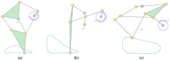
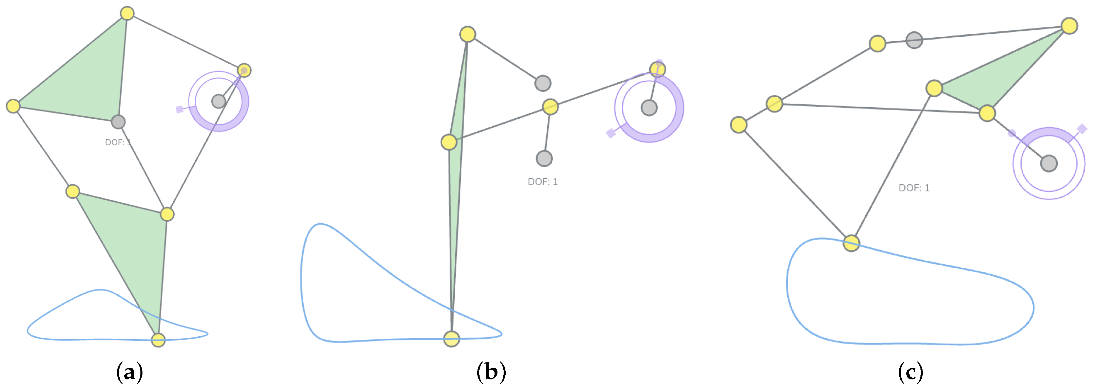
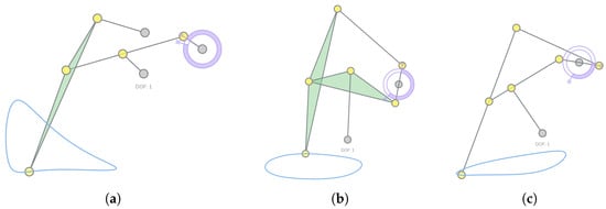
Planar 1-DOF walking linkages have a rich history and continue to attract interest in robotics and mechanism design. Classic examples include Chebyshev-type leg mechanisms, Klann six-bar linkages, and Theo Jansen’s multi-link walkers [3,4,5,6]. Figure 1 shows these three existing walking linkages.

Figure 1. The figure shows three existing walking linkages drawn and simulated in MotionGen [1]: (a) Jansen Linkage, (b) Klann Linkage, (c) Trotbot Linkage.

Historically, many of these designs relied heavily on intuition, manual iteration, and physical prototyping. In contrast, modern robotics and mechanism design increasingly demand computational tools that can systematically explore large design spaces while enforcing task-specific constraints (e.g., ground contact behavior, clearance, and gait-like features). Walking mechanisms provide an especially useful testbed because successful designs must satisfy multiple interacting criteria beyond reproducing a single coupler curve.

Mechanism synthesis aims to determine mechanism topology and dimensional parameters to satisfy prescribed path, motion, or function requirements, as treated extensively in classical synthesis texts [7,8]. Analytic approaches such as kinematic mapping and algebraic fitting provide unified formulations for motion synthesis and have been extended toward simultaneous type-and-dimension synthesis [9]. To make these synthesis techniques practical, interactive tools have been developed, notably MotionGen for real-time four-bar motion generation with pose and geometric constraints [2].

More recently, there has been a growing interest in combining large-scale data generation with machine learning for mechanism design. Prior work proposed learning-based synthesis of defect-free mechanisms and methods to handle uncertain user inputs, including image-based representations of input curves and invariant/normalized representations of coupler curves [10,11,12]. Large datasets have accelerated data-driven design, e.g., the LINKS dataset of 100M planar linkage mechanisms [13] and a curated dataset of nearly 3M single-DOF planar 4-, 6-, and 8-bar mechanisms with open/closed coupler curves [14]. In rehabilitation-oriented motion design, representative pipelines combine data generation, learned representations, and retrieval/selection to produce multiple candidate mechanisms under practical constraints [15]. Beyond Variational Auto Encoder (VAE)-style embeddings and retrieval, other learning paradigms have also been explored, including conditional GANs under constraints [16], reinforcement-learning-based synthesis [17], graph-based generative approaches for linkage graphs [18], sequence-model-based mechanism design automation [19], and conditional generative modeling applied to six-bar synthesis [20].

Frequently, mechanism design problems are reduced to finding suitable combinations of links and joints that generate a given path, such as that of a foot point during average walking motion. However, path-matching alone is often insufficient for broader robotics design tasks requiring satisfying multiple and often conflicting design specifications. First, many applications admit families of functional mechanisms rather than a single best-fitting curve; optimizing only for a target trajectory can overlook alternatives whose coupler curves differ slightly yet still satisfy the task. Second, existing pipelines do not provide a general method to filter or curate large datasets using application-specific geometric criteria, especially when those criteria involve more than curve similarity. Third, practical design problems impose hard feasibility constraints that must be satisfied in addition to producing a plausible path. For walking mechanisms, examples include requiring a closed foot trajectory, enforcing a sufficiently flat stance phase for ground contact and propulsion, ensuring adequate step height and step length, and preventing non-foot joints or links from intersecting the ground during motion. These requirements motivate a synthesis pipeline that treats “walking-ness” as a constrained objective rather than as a byproduct of path similarity.

To overcome these limitations while leveraging the scalability of data-driven approaches, we propose a design-criteria-driven synthesis pipeline that treats “walking-ness” as multi-criteria satisfaction rather than path similarity. Unlike pure learning methods that excel at efficient search but can struggle with hard constraints, our approach combines large-scale simulation with explicit geometric filters, offering complementary advantages: (1) guaranteed geometric feasibility through direct constraint checking, (2) sufficient sampling within the constrained region, (3) explicit criteria formulation allowing transparent tuning for specific applications, and (4) interpretable failure modes when mechanisms are rejected. This approach maintains scalability while introducing application-specific intelligence through targeted filtering criteria and soft optimization of near-feasible designs. As a result, our pipeline provides a verified training dataset with explicit feasibility boundaries that can bootstrap and validate learned models.

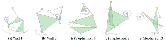
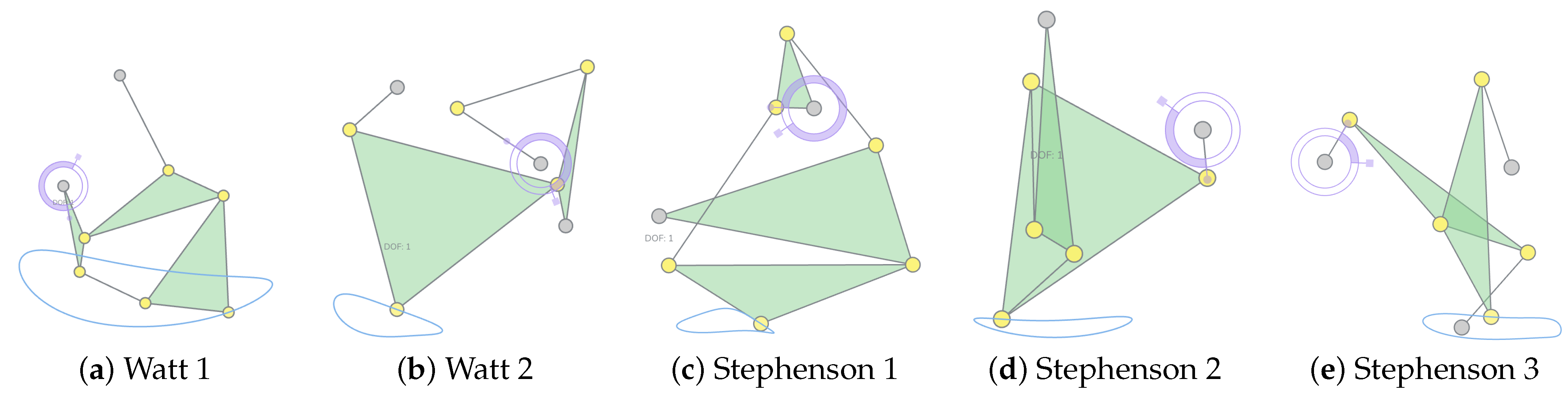
Implementation scope: We demonstrate this pipeline on four types of planar four-bar mechanisms with revolute (R) and prismatic (P) joints—RRRR, RRRP, RRPR, and PRPR—and five six-bar mechanisms, classified into two Watt types and three Stephenson types (Figure 2). Additionally, we include different variants of these five types where coupler points are placed on different links. For details on these kinematic structures, see [21]. The resulting dataset provides not just feasible mechanisms but also the geometric criteria that define their feasibility, enabling both direct application and further learning-based refinement.

Figure 2. Five types of six-bar mechanisms in our work.

Although developed and demonstrated for walking, the methodology is intended to generalize to other robotics mechanism design tasks where feasibility and performance are defined by geometric/kinematic criteria. The main contributions of this paper are:

1.

Geometric constraint formulation for walking mechanisms: We propose a scalable computational pipeline to identify planar walking mechanisms from randomly generated linkages by enforcing five explicit geometric criteria.

2.

Large-scale simulation and dataset filtering: We generate a large-scale dataset by sampling linkage joint coordinates from an explicit distribution (uniform within fixed bounds) and simulating each candidate across 25 structural subtypes. Then, we evaluate approximately ${10}^8$ candidates in total (4 M per subtype) and retain $23,250$ feasible walking mechanisms after filtering. Our implementation runs efficiently on High-Performing Computing resources (e.g., ∼5–6 h per 4 million candidates for a representative subtype on the SeaWulf computing cluster from Stony Brook University (Website for SeaWulf: https://rci.stonybrook.edu/HPC/understanding-SeaWulf (accessed on 21 January 2026)).

3.

Optimization-based refinement of near-feasible designs: We further improve walkability via a derivative-free optimization that adjusts only ground-violating joints. We use Differential Evolution [22] with penalty-based constraint handling to minimize a composite objective that discourages invalid stance detection, ground penetration, and poor trajectory closure, and we terminate after a fixed evaluation budget or when the best objective value stalls.

The remainder of this paper is arranged as follows. Section 2 describes the dataset generation, filtering procedure, and the design-driven objective used for fine-tuning. Section 3 reports filtered dataset statistics and representative walking results, and evaluates the effectiveness of the optimization step. Section 4 concludes with a discussion of limitations and implications for broader robotics mechanism design.

2. Methodology

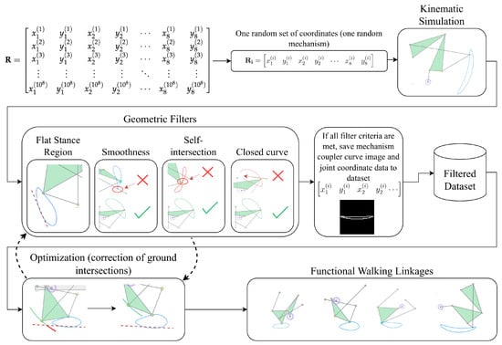
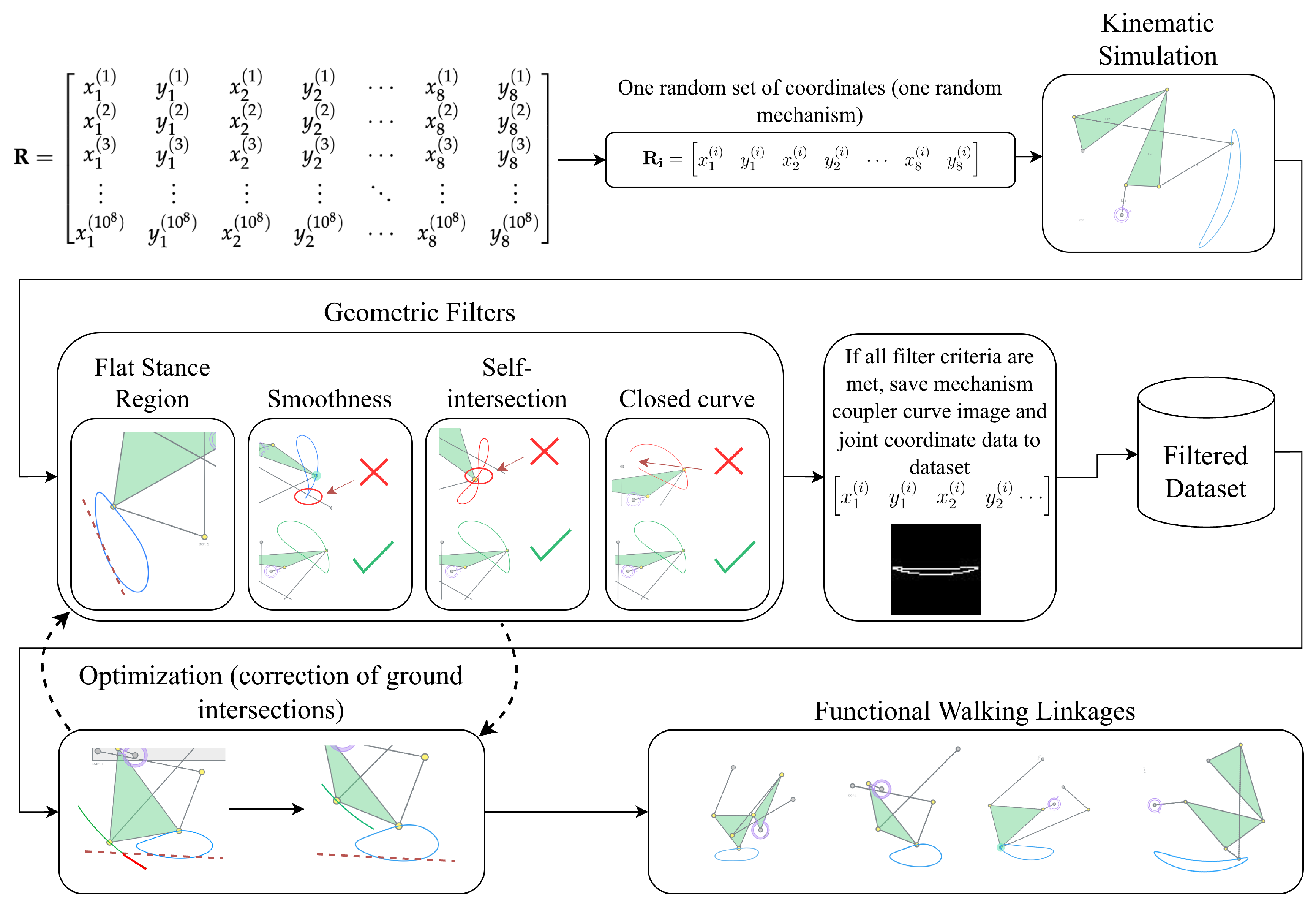
The methodology developed in this work builds upon an existing mechanism simulation framework by Lyu et al. [2]. The overall workflow consists of three stages: simulation (Section 2.1), dataset filtering (Section 2.2), and fine-tuning (Section 2.3) (Figure 3).

Figure 3. Design pipeline for walking mechanism generation, filtering, and optimization. The dashed arrows represent an iterative refinement loop: near-feasible mechanisms from filtering are optimized, with successful candidates evaluated using the filters again.

Neither random sampling nor numerical optimization alone is sufficient. In a design space with at least ten dimensions (RRRR, for example), sampling only produces suboptimal solutions. Meanwhile, nonlinear optimization initialized from random parameters frequently fails to converge, incurring substantial computational cost. We therefore combine the two: sampling provides good initial guesses, and optimization refines them to best-fit mechanisms efficiently.

Therefore, in the simulation stage, we sample large numbers of randomized mechanism parameters and perform kinematic simulation to generate candidate motions for the selected mechanism families. In the filtering stage, we evaluate a set of walking-specific geometric criteria on the simulated motions and retain only candidates that satisfy the feasibility conditions, resulting in a curated dataset of potentially walkable mechanisms. Finally, the fine-tuning stage refines near-feasible candidates by adjusting design parameters to correct geometric violations that prevent walking (e.g., non-foot joints intersecting the ground). This refinement is formulated as an optimization problem with a custom, design-driven objective constructed from the same geometric criteria together with a measure of walking effectiveness. Figure 3 provides an overview of the complete pipeline.

2.1. Simulation

We use the simulator developed by Lyu et al. [2] to generate kinematic trajectories from randomized initial joint configurations. Given initial joint coordinates and a specification of the mechanism type, the simulator outputs the coupler curves (trajectories) of all joints over a full motion cycle.

To support large-scale sampling, we first generate random coordinate values and store them in a matrix $\mathbf{R}\in {\mathbb{R}}^{{10}^8\times 16}$ prior to simulation. These values are between $-10$ to 10, because we standardize the simulation result with respect to the coupler path using the method in [15] so that the curve is invariant to translation, rotation, scaling, and reflection. Additionally, unlike [23], which uses the Fourier Descriptor (FD), the method in this work does not require full rotation or a fixed number of points.

Each row of $\mathbf{R}$ contains 16 scalars, interpreted as 8 planar $(x,y)$ pairs, which is sufficient to provide randomized coordinates for all joints required by the 4-bar and 6-bar families considered in this work (five joints for 4-bar mechanisms, and seven or eight joints for6-bar mechanisms).

$$\mathbf{R}=\left[\begin{array}{ccccccc}{x}_1^{\left(1\right)}& y_1^{\left(1\right)}& x_2^{\left(1\right)}& y_2^{\left(1\right)}& \dots & x_8^{\left(1\right)}& y_8^{\left(1\right)}\\ x_1^{\left(2\right)}& y_1^{\left(2\right)}& x_2^{\left(2\right)}& y_2^{\left(2\right)}& \dots & x_8^{\left(2\right)}& y_8^{\left(2\right)}\\ x_1^{\left(3\right)}& y_1^{\left(3\right)}& x_2^{\left(3\right)}& y_2^{\left(3\right)}& \dots & x_8^{\left(3\right)}& y_8^{\left(3\right)}\\ ⋮& ⋮& ⋮& ⋮& \ddots & ⋮& ⋮\\ x_1^{\left({10}^8\right)}& y_1^{\left({10}^8\right)}& x_2^{\left({10}^8\right)}& y_2^{\left({10}^8\right)}& \dots & x_8^{\left({10}^8\right)}& y_8^{\left({10}^8\right)}\end{array}\right].$$

The kinematic structure of each mechanism type is encoded by three matrices, $\mathbf{B}$, $\mathbf{S}$, and $\mathbf{I}$, following the representation in [2]. These mechanisms are collectively saved with their matrices in a dictionary (See a definition of BSIdict in [21]).

The binary incidence matrix $\mathbf{B}$ specifies link–joint connectivity. Formally, the $\mathbf{B}$ matrix is defined as

$$\mathbf{B}\in {\{0,1\}}^{\ell \times n},$$

where n is the number of joints, ℓ is the number of link-incidence rows (including the ground row), and $b_{ij}$ denotes the element in row i and column j.

The first row in the matrix B is defined as

$${\mathbf{b}}_1=[b_{11},b_{12},\dots ,b_{1n}],b_{1j}=\left\{\begin{array}{cc}1\hfill & \mathrm{if}\mathrm{joint}j\mathrm{is}\mathrm{grounded},\hfill \\ 0\hfill & \mathrm{otherwise}.\hfill \end{array}\right.$$

while the rows 2 through l are defined as For each link row $i=2,\dots ,\ell$,

$${\mathbf{b}}_i=[b_{i1},b_{i2},\dots ,b_{in}],b_{ij}=\left\{\begin{array}{cc}1\hfill & \mathrm{if}\mathrm{joint}j\mathrm{lies}\mathrm{on}\mathrm{link}i,\hfill \\ 0\hfill & \mathrm{otherwise}.\hfill \end{array}\right.$$

For mechanism types that include prismatic joints (i.e., collinearity constraints), the corresponding $\mathbf{S}$ matrix is non-empty. Each row of $\mathbf{S}$ stores a triplet of joint indices that must remain collinear. For example, if joints $\mathbf{P}$, q, and r are constrained to lie on the same line, then the row $[p,q,r]$ appears in $\mathbf{S}$.

The actuator specification is stored in the $\mathbf{I}$ matrix. Similar to $\mathbf{S}$, each row of $\mathbf{I}$ contains three joint indices defining the actuation constraint, together with a fourth entry indicating actuator type. For a rotary actuator that enforces the angle between vectors ${\overrightarrow{v}}_{qp}$ and ${\overrightarrow{v}}_{qr}$ (with joint indices $\mathbf{P}$, q, and r), the corresponding row is $[p,q,r,0]$. For a linear actuator, ${\overrightarrow{v}}_{qr}$ defines the reference direction and ${\overrightarrow{v}}_{qp}$ defines the actuated length, yielding the row $[p,q,r,1]$.

Given a set of random joint coordinates together with the matrices $\mathbf{B}$, $\mathbf{S}$, and $\mathbf{I}$ for a selected mechanism type, the simulator outputs a tensor $\mathbf{P}\in {\mathbb{R}}^{2\times m\times N}$, where m is the number of joints and N is the number of simulated time steps. The first dimension (of size 2) corresponds to $(x,y)$ coordinates. We write

$$\mathbf{P}=\left[{\mathbf{P}}^{\left(0\right)},{\mathbf{P}}^{\left(1\right)},\dots ,{\mathbf{P}}^{(N-1)}\right],$$

where each

$${\mathbf{P}}_i=\left[\begin{array}{ccc}{x}_1^{\left(i\right)}& \dots & x_m^{\left(i\right)}\\ y_1^{\left(i\right)}& \dots & y_m^{\left(i\right)}\end{array}\right]\in {\mathbb{R}}^{2\times m}$$

contains all joint positions at simulation step i. From this tensor, we extract the trajectory of the coupler point and denote it by

$$P=\{P^{\left(0\right)},P^{\left(1\right)},\dots ,P^{\left(n\right)}\},P_i\in {\mathbb{R}}^2,$$

where $P_i$ is the planar position of the coupler at simulation step i, and $n=N-1$.

2.2. Dataset Filtering

After simulating each mechanism from randomized parameters, we evaluate a set of geometric criteria to determine whether the candidate should be retained in the dataset. These criteria are derived from common design considerations for planar 1-DOF walking mechanisms reported in prior design-oriented studies and articles [24,25,26]. Only mechanisms that satisfy all required feasibility conditions are saved to the database for downstream analysis and refinement.

The adopted criteria are:

1.

Closed foot trajectory: the selected coupler curve (foot point) must form a closed, periodic curve over a full actuation cycle (Section 2.2.1).

2.

No self-intersection: the coupler curve must be a simple closed curve (i.e., it must not intersect itself) (Section 2.2.1).

3.

Bounded curvature/smoothness: the trajectory must not contain excessively sharp corners or abrupt direction reversals; equivalently, curvature and/or the turning angle between successive samples must remain below a specified threshold (Section 2.2.2).

4.

Existence of a stance segment: the trajectory must contain a sufficiently long “flat” portion suitable for ground contact during stance (Section 2.2.3).

5.

Stance proportion constraint: depending on the intended robot configuration (e.g., the number of legs operating in parallel), the stance segment must occupy at least a minimum fraction of the full cycle (duty factor) (Section 2.2.3).

6.

Ground clearance for non-foot joints: when the mechanism is oriented such that the stance segment lies on the ground line, no other joint trajectory (and, if applicable, the mechanism geometry) may intersect the ground (Section 2.2.4).

Motivation for geometric criteria: Each filtering criterion corresponds to a physical requirement for walking. Closure ensures a periodic, continuous motion for repeated stepping. Self-intersection avoidance prevents ambiguous foot positions, which could interfere with the stance portion of a step. Smoothness corresponds to foot acceleration profiles; sharp, angled portions in the coupler curve would create uneven acceleration. Flat stance segments enable ground contact and propulsion. Ground clearance prevents mechanical interference. These geometric proxies allow efficient screening before expensive dynamic simulation.

Within these algorithms, many thresholds are used to calculate the different properties of the mechanisms. They are outlined in Appendix A.

2.2.1. Closed Coupler Curve and Self-Intersection Test

  To ensure that the simulated coupler curve defines a valid closed foot trajectory for walking, we perform two preliminary checks: (i) closure and (ii) self-intersection (Algorithm 1). A walking trajectory must be periodic; otherwise, the mechanism cannot sustain continuous stepping over repeated cycles, even if other criteria are satisfied. In addition, we reject self-intersecting trajectories because a self-intersection implies that the curve is not a simple closed path; this can yield ambiguous contact/stance regions and non-unique horizontal positions for the same phase, which is undesirable for stable forward walking.

Algorithm 1: Coupler Curve Closure and Self-Intersection Tests

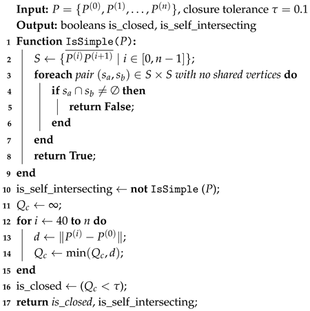For the classic four-bar linkages, analytical criteria such as Grashof’s condition can be used to determine the existence of a continuously rotating crank. However, for six-bar topologies (e.g., Watt and Stephenson types), the Grashof condition is not applicable. Since the objective of this work is to identify mechanisms that generate closed and periodic walking trajectories, closure is verified directly at the trajectory level by simulating one full input cycle and ensuring periodic return to the initial configuration within numerical tolerance. This approach guarantees closed output behavior for all types of kinematic structures.

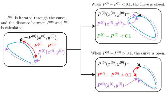
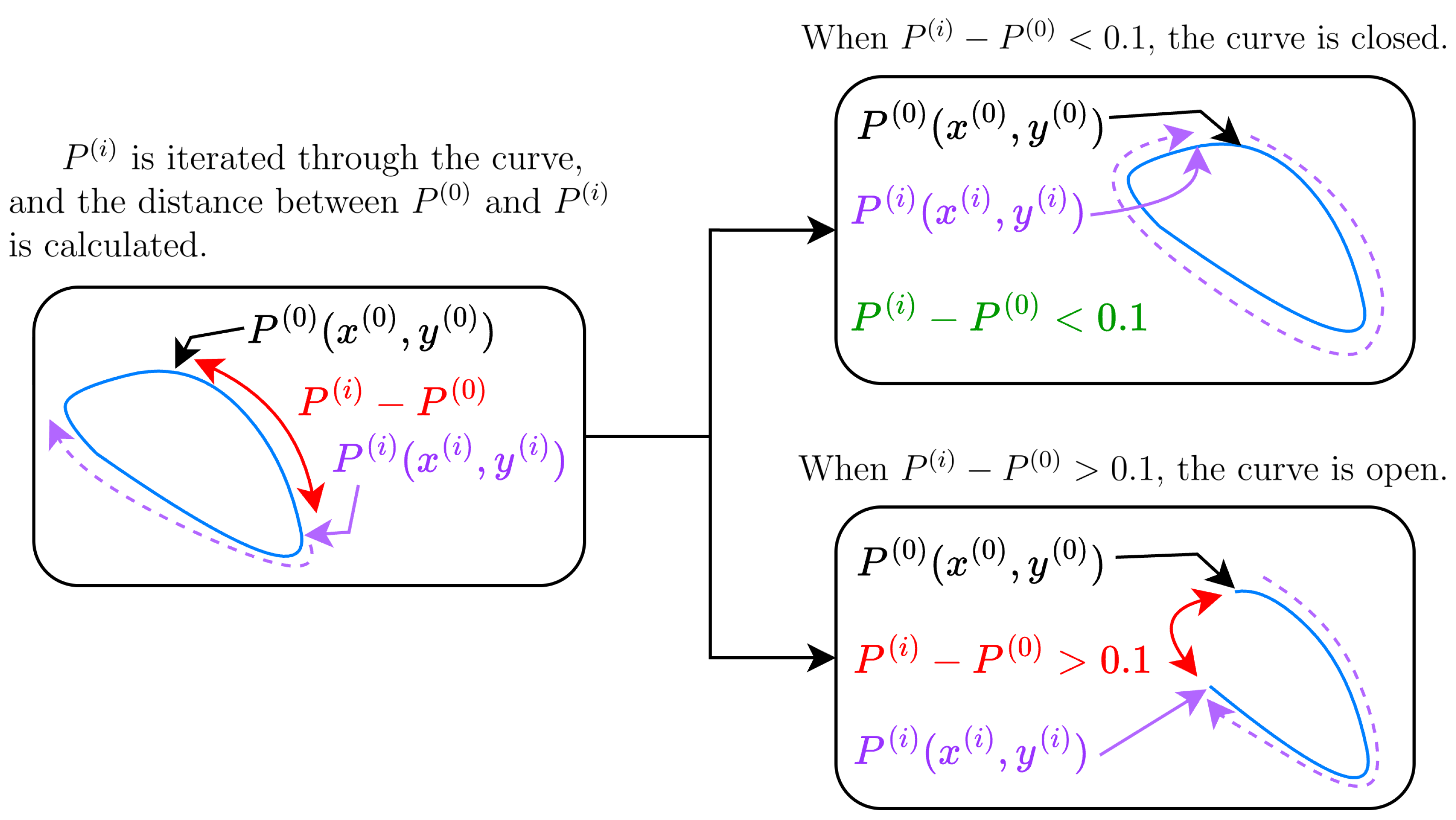
Closure test. Let $P=\{P^{\left(0\right)},P^{\left(1\right)},\dots ,P^{\left(n\right)}\}$ denote the sampled points of the coupler trajectory returned by the simulator. Rather than comparing only the first and last samples, we search for a return-to-start event within the trajectory, since some simulations may contain multiple cycles or partial overlaps, in which case the final sample may not coincide with a true cycle boundary. Specifically, we compute the minimum distance from the start point $P_0$ to later samples $P_i$ while skipping an initial prefix to avoid trivial near-start matches:

$$Q_c=\underset{i\ge i_{min}}{min}{\parallel P^{\left(i\right)}-P^{\left(0\right)}\parallel }_2,$$

where $i_{min}=40$ in our implementation (Figure 4), and $n=512$ is the total number of samples. We declare the trajectory to be closed if $Q_c<\tau$, where $\tau =0.1$ is a tolerance that admits small numerical gaps while still rejecting clearly open curves. Although a self-intersecting trajectory may also yield a small value of $Q_c$, such cases are subsequently rejected by the self-intersection test.

Figure 4. The closure test performed on the coupler curve in Algorithm 1. The blue curve is the coupler curve that we are evaluating, the red line indicates the distance $P^{\left(i\right)}-P^{\left(0\right)}$, and the purple dashed line indicates the iteration through the curve.

Self-intersection test. Let $P=\{P^{\left(0\right)},P^{\left(1\right)},\dots ,P^{\left(n\right)}\}$ denote the sampled planar trajectory, and define the associated polyline segments

$$S=\{\overline{P^{\left(i\right)}{P}^{(i+1)}}\mid i=0,\dots ,n-1\}.$$

The curve is declared self-intersecting if there exist two non-adjacent segments $\overline{P^{\left(i\right)}{P}^{(i+1)}}$, $\overline{P^{\left(j\right)}{P}^{(j+1)}}$$\in S$ with $|i-j|>1$ such that

$$\overline{P^{\left(i\right)}{P}^{(i+1)}}\cap \overline{P^{\left(j\right)}{P}^{(j+1)}}\ne \varnothing .$$

Adjacent segments sharing a common endpoint are excluded from this test. In practice, this amounts to checking all pairs of non-adjacent segments for intersection using standard segment–segment intersection predicates. If any such intersection is found, the boolean flag is_self_intersecting is set to True and the curve is rejected.

2.2.2. Smoothness Test

We assess the smoothness of a coupler curve using its curvature. Large curvature values correspond to sharp turns or abrupt changes in direction, which are generally undesirable for walking trajectories.

To reduce sensitivity to sampling noise, we smooth the sampled $(x,y)$ coordinates using a one-dimensional Gaussian filter. We then compute first- and second-order derivatives via numerical gradients and evaluate the curvature at each sample point as

$$\kappa ={\displaystyle \frac{\left|x^{\prime }{y}^{″}-y^{\prime }{x}^{″}\right|}{{\left(x^{\prime 2}+y^{\prime 2}\right)}^{3/2}}}.$$

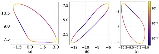
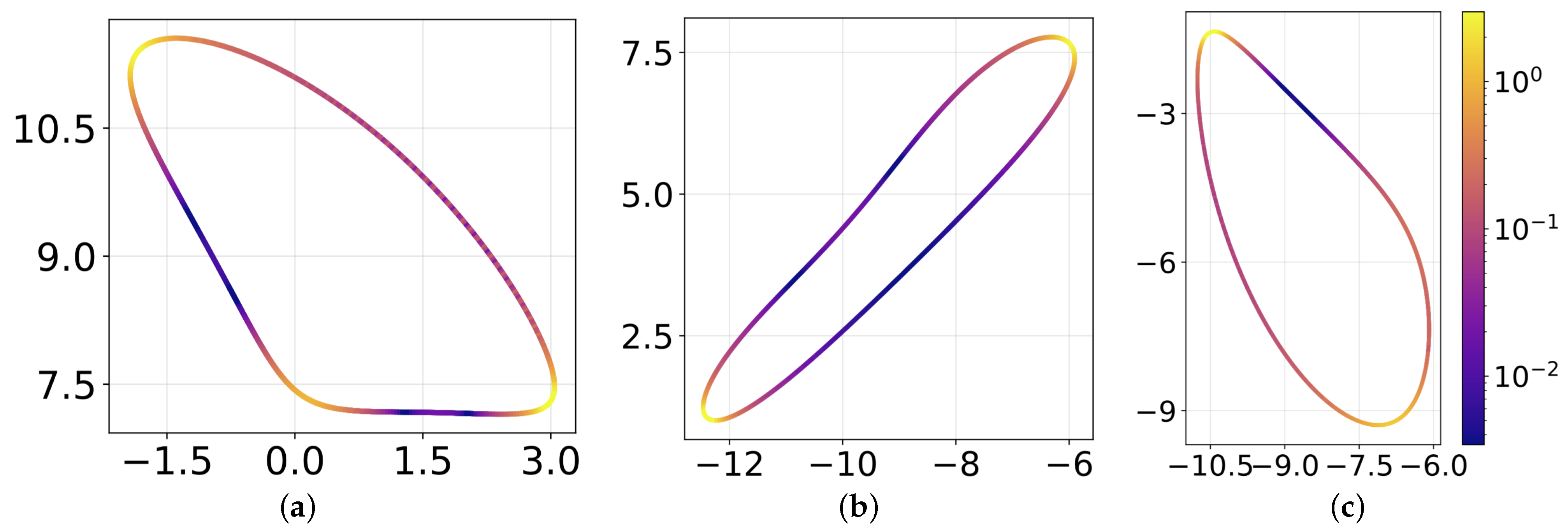
If the maximum curvature along the curve exceeds a threshold $\alpha$, the trajectory is rejected as non-smooth. In our experiments, $\alpha =15$ provided an effective cutoff for eliminating trajectories with excessively sharp features. Algorithm 2 summarizes the procedure, and Figure 5 visualizes three example coupler curves with curvature values shown by color.

Algorithm 2: Smoothness Test via Curvature Thresholding.

Input: Coupler coordinates $P=\left\{(x_i,y_i)\right\}$, smoothness threshold $\alpha$

Output: has_sharp_corners

1 $x,y\leftarrow$ gaussian_filter_1D($\mathbf{P}$, smoothing $\sigma =1$)

2 Compute $x^{\prime }=\nabla x$, $y^{\prime }=\nabla y$, $x^{″}=\nabla x^{\prime }$, $y^{″}=\nabla y^{\prime }$

3 ${\kappa }_i={\displaystyle \frac{|x_i^{\prime }{y}_i^{″}-y_i^{\prime }{x}_i^{″}|}{{(x_i^{\prime 2}+y_i^{\prime 2})}^{3/2}}}$∀i

4 has_sharp_corners ← true_if_any(${\kappa }_i>\alpha$)

5 return has_sharp_corners

Figure 5. The figure shows three example coupler curves with curvature color-mapped along their lengths. A log scale for curvature is used for better visualization. (a) is the first example, (b) is the second example, and (c) is the third example.

2.2.3. Flatness Detection: Stance, Contact, and Ground Model

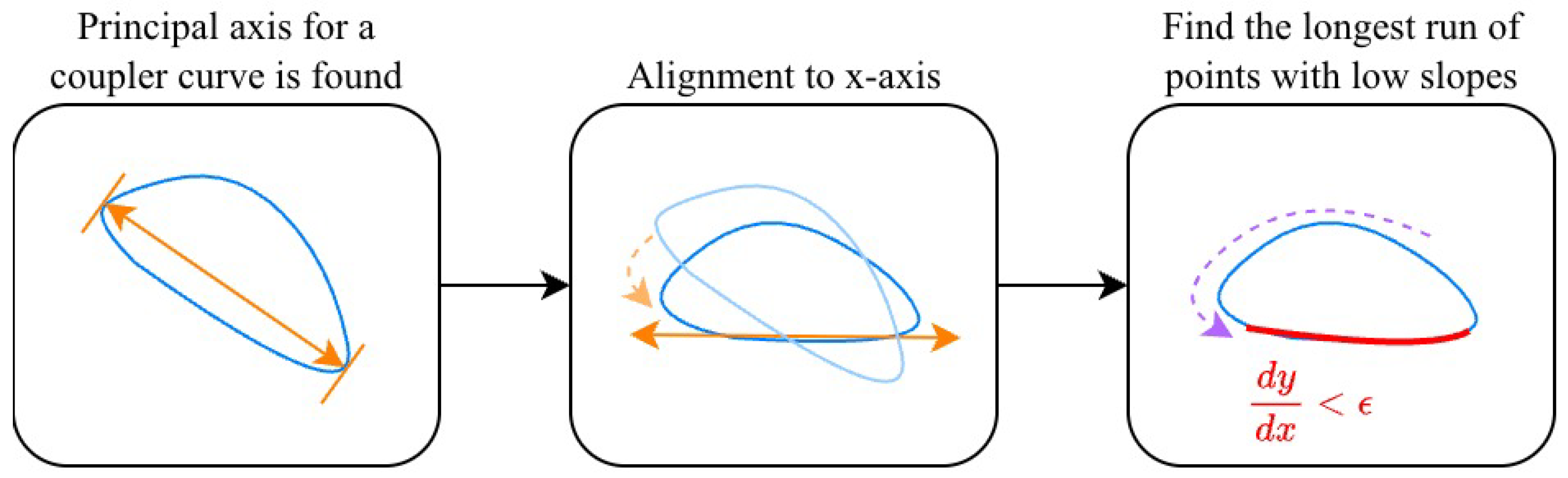
In this work, we define stance and ground contact using a purely geometric approximation based on the shape of the foot trajectory. The selected coupler point is treated as the contact point, and the ground is modeled as a straight line inferred from the flat portion of the trajectory via least-squares fitting. To reason about flatness consistently, we analyze trajectories in a ground-aligned coordinate frame obtained by rotating the curve so that its dominant direction of motion is horizontal. The stance phase is then identified as the longest near-horizontal segment of the trajectory in this aligned frame. This definition provides a practical proxy for foot-ground contact and does not attempt to model contact forces, slip, or dynamics.

The flat portion of the coupler curve corresponds to the stance phase of walking, during which the foot remains approximately in contact with the ground and provides support and propulsion.

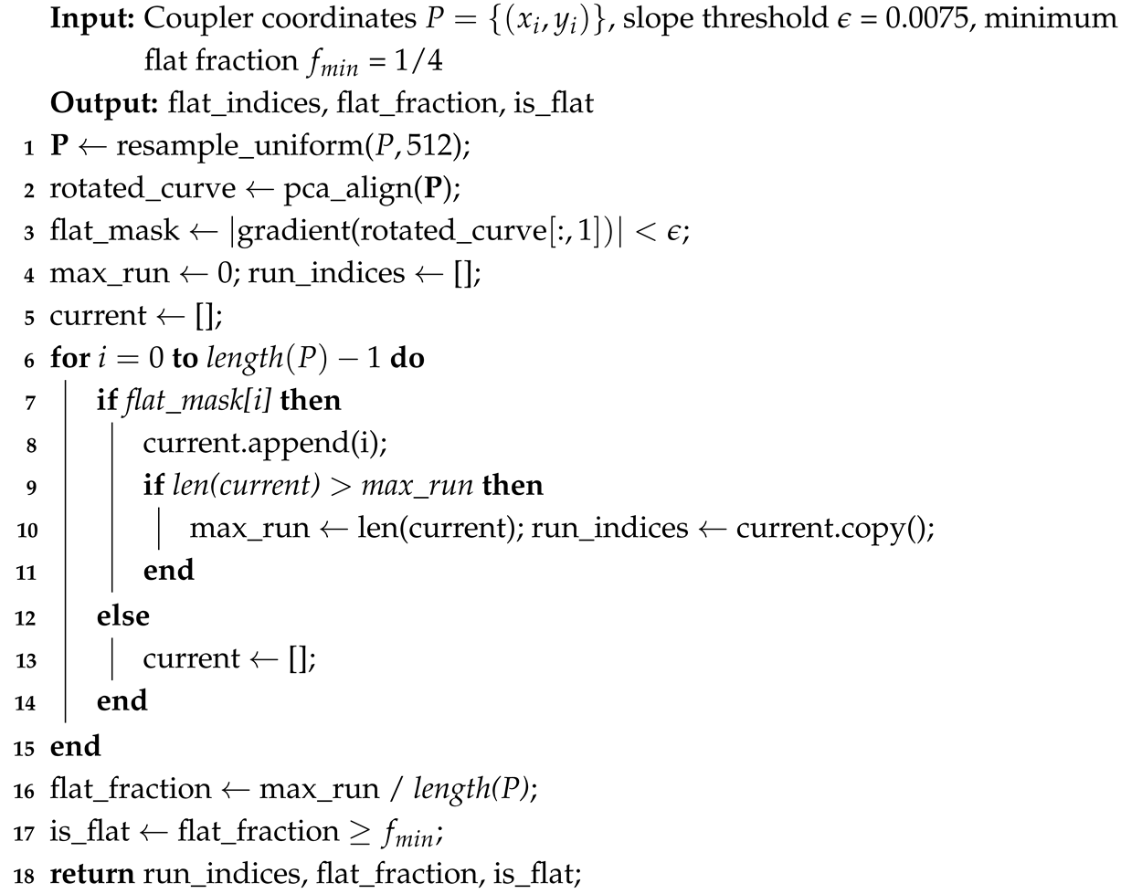
We detect this stance segment by (i) rotating the trajectory so that the dominant direction of variation aligns with the x-axis, and (ii) identifying regions with sufficiently small slope in the rotated frame.

To align the curve, we apply Principal Component Analysis (PCA) to the sampled $(x,y)$ points and rotate the trajectory such that the first principal component (the direction of greatest variance) is aligned with the x-axis. For walking-like trajectories, the stance segment is typically the longest near-linear portion and therefore dominates the variance, making this alignment a practical approximation. After alignment, we compute the slope, and the points with slope magnitude below a threshold are labeled as “flat”; in our implementation, we use $ϵ=0.0075$. See Figure 6 for illustration.

Figure 6. Visualization of the flatness detection by aligning the principal axis and detecting low slope regions. The orange line indicates the principal axis, the dashed purple arrow shows the algorithm iterating over the coupler curve, and the red portion indicates the run of points with low slopes below the slope threshold $ϵ$.

We then identify contiguous runs of flat points and define the flatness fraction as the length of the longest flat run normalized by the total curve length (Algorithm 3). The minimum required flatness fraction depends on the desired duty factor and the number of legs operating in parallel. As a simple guideline, if N identical legs are phase-shifted to provide continuous ground contact, each leg typically requires a stance fraction of at least $1/N$ of the cycle. In this study, we accept a trajectory if at least one quarter of the cycle is classified as flat (flatness fraction $\ge 0.25$), corresponding to a nominal requirement of $N\le 4$ legs for continuous contact under ideal phase scheduling. Additional legs may be needed in practice for stability and balance, which are hardware-level considerations beyond the scope of this work.

Algorithm 3: Flat Region, indices, and flatness fraction detection via PCA Alignment

While vertical deviation constraints could limit absolute displacement along the y-axis, they do not directly suppress local oscillatory behavior within a tolerance band. By monitoring the derivative ${\displaystyle \frac{dy}{dx}}$ during the stance phase, the method enforces directional consistency and limits small oscillations that could otherwise occur while remaining within vertical bounds.

The derivative is computed using sufficiently fine discretization of the trajectory, and numerical stability was verified empirically during implementation.

2.2.4. Ground Intersection Test

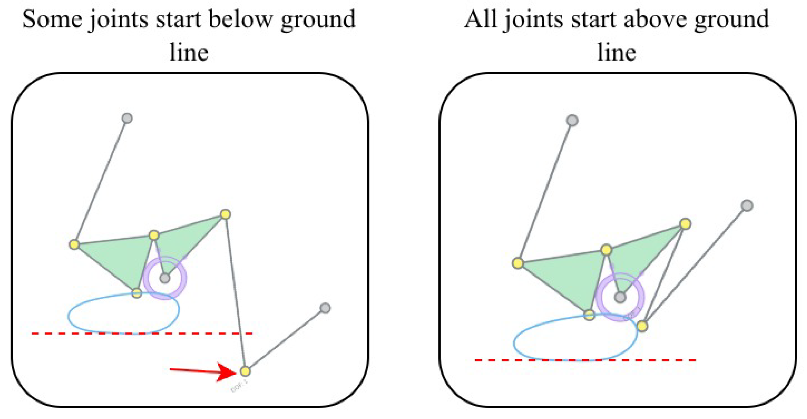
The final test verifies ground clearance: when the mechanism is oriented such that the foot is supported by its flat stance segment, no other joint trajectory should intersect the ground. We approximate the ground by a line ℓ fitted in the least-squares sense to the detected stance-phase foot points. Specifically, ℓ is chosen to minimize the sum of squared orthogonal distances to these points. We then compute the signed distance of every joint position to ℓ, with the sign chosen so that the supporting foot points lie on the zero or negative side. The mechanism passes the test if, for all time steps, every non-foot joint remains strictly on the positive (clearance) side of ℓ. See Algorithm 4 and Figure 7. In this algorithm, m and b are the slope and y-intercept, respectively.

Algorithm 4: Joint-Ground Intersection Test.

Input: Coupler path $P=\left\{(x_i,y_i)\right\}$, joint coordinates $J=\left\{(x_i,y_i)\right\}$, flat indices $I_{\mathrm{flat}}$

Output: isGroundClear

1 $(m,b)\leftarrow$ linear_regression($P_{I_{\mathrm{flat}}}$)

2 $d_{\mathrm{path}}\leftarrow P_y-(m{P}_x+b)$

3 $\mathrm{majoritySign}\leftarrow \mathrm{sign}(\sum d_{\mathrm{path}})$

4 $d_{\mathrm{joints}}\leftarrow J_y-(m{J}_x+b)$

5 isGroundClear ← all(sign($d_{\mathrm{joints}}$) is equal to majoritySign)

6 return isGroundClear

Figure 7. This figure shows an example mechanism that does not pass the ground intersection test (left), and one that passes the test (right).

2.3. Optimization Methodology

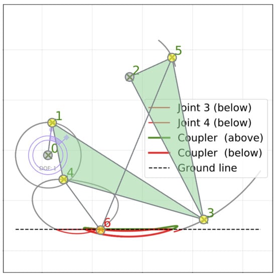
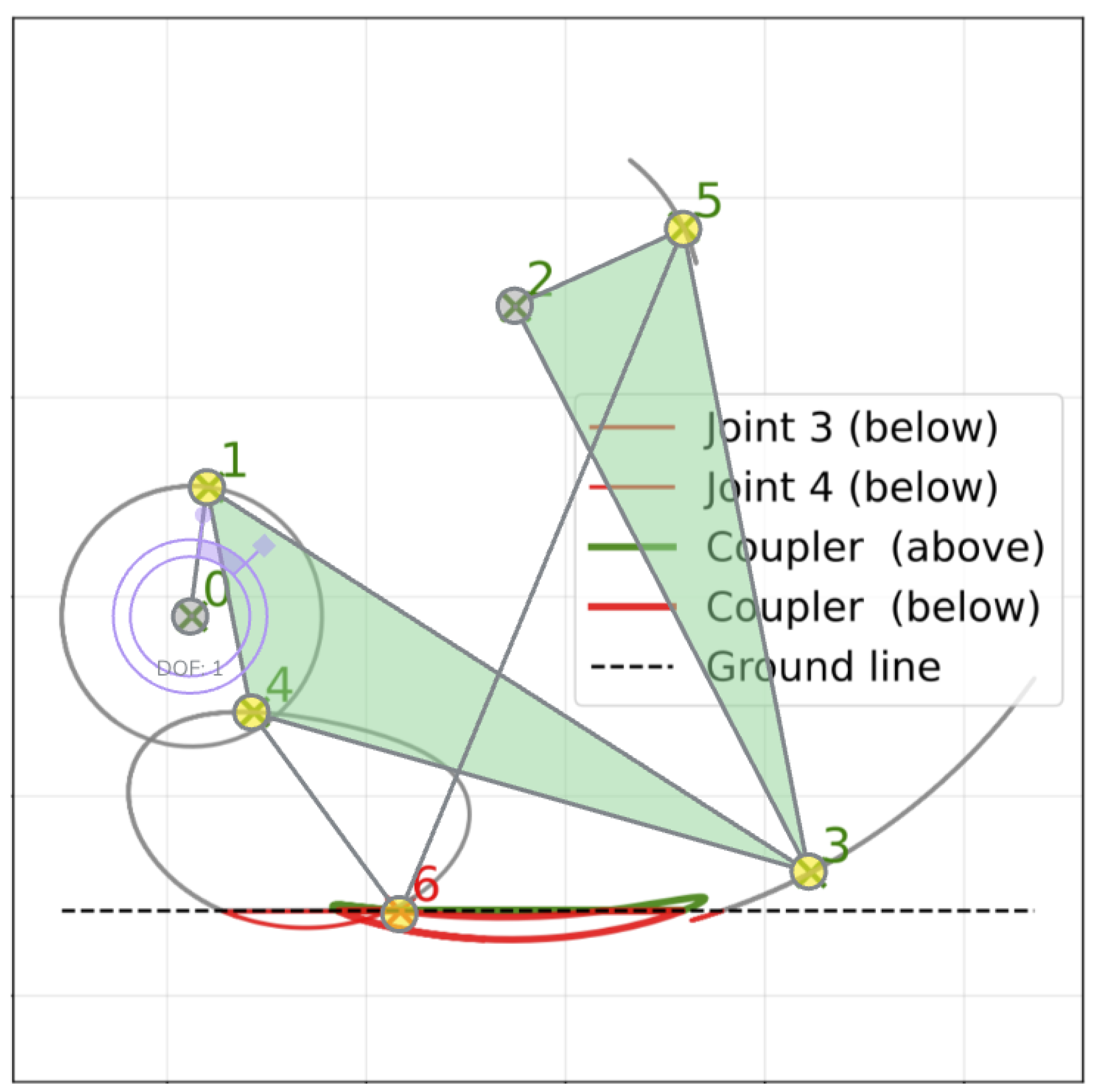
Even after passing the geometric filters, some candidates still fail functionally because one or more non-foot joints intersect the best-fit ground line estimated from the stance segment of the foot trajectory. Physically, this corresponds to linkages whose joints collide with the ground, preventing locomotion (Figure 8).

Figure 8. An example of a near-walking 6-bar mechanism. Initial joint positions are shown as green X’s, and all joint trajectories are shown. In this specific mechanism, joints 0 and 2 are grounded. The coupler curve passes through all criteria; however, joints 3 and 4 pass through the ground line. The offending portion intersecting the ground line is marked in red.

In practice, many of these near-feasible mechanisms require only small geometric adjustments to resolve the collision. Modest perturbations of one or two joint locations can often restore ground clearance while preserving the overall walking-like trajectory. Discarding such candidates would therefore eliminate designs that are close to feasible and potentially valuable.

For this reason, we retain a subset of near-feasible mechanisms that do not strictly satisfy the ground-clearance condition and subsequently refine them through an optimization-based fine-tuning step (Algorithm 5).

Algorithm 5: Optimization of Mechanisms with Ground Intersections

Input: Initial parameters $\theta$, mechanism representation matrices $\mathbf{B}$, $\mathbf{S}$ and $\mathbf{I}$, flatness threshold $ϵ$

Output: Optimized trajectories ${\mathbf{P}}^{*}$, and configuration ${\theta }^{*}$

1 Simulate to obtain all joint trajectories $\mathbf{P}=\mathrm{simulate}(\theta ,\mathbf{B},\mathbf{S},\mathbf{I})$(Section 2.1)

2 Resample $\mathbf{P}$ uniformly along its path.

3 Retrieve coupler curve $CC$ from trajectory.

4 Compute ground line $(m,b,s)=\mathrm{compute}\_\mathrm{Fground}\_\mathrm{line}\_\mathrm{with}\_\mathrm{sign}(CC)$

5 Identify joints intersecting the ground:        ${\mathrm{J}}_{adj}=\mathrm{find}\_\mathrm{joints}\_\mathrm{below}\_\mathrm{ground}(\mathbf{P},m,b,s)$

6 Define optimization variables $\varphi$ (offsets for joints in ${\mathrm{J}}_{adj}$).

7 Set search bounds $\varphi \in {[-5,5]}^{2|{\mathrm{J}}_{adj}|}$.

8 Define error function $E\left(\varphi \right)$:

9      For a given $\varphi$, obtain mechanism initial state ${\theta }^{\prime }=\mathrm{apply}(\theta ,\varphi ,{\mathrm{J}}_{adj})$.

10    Obtain new trajectories ${\mathbf{P}}^{\prime }=\mathrm{simulate}({\theta }^{\prime },\mathbf{B},\mathbf{S},\mathbf{I})$.

11    Compute geometric penalties $(I,W,L,C)$ from ${\mathbf{P}}^{\prime }$ and return total error        $E\left(\varphi \right)=I+W+L+C$.

12 Minimize $E\left(\varphi \right)$ using Differential Evolution until convergence:

13 ${\varphi }^{*}=arg{min}_{\varphi }E\left(\varphi \right)$

14 Apply optimal offsets ${\varphi }^{*}$ to ${\theta }^{*}$ and regenerate optimized trajectories        ${\mathbf{P}}^{*}=\mathrm{simulate}({\theta }^{*},\mathbf{B},\mathbf{S},\mathbf{I})$.

15 return ${\mathbf{P}}^{*}$, ${\theta }^{*}$

Specifically, we identify the set $J_{\mathrm{adj}}$ of joints whose simulated trajectories violate the ground-clearance test. We optimize only these joints by applying planar offsets $\varphi$ to theirinitial coordinates, keeping all other joints fixed. The search domain is $\varphi \in {[-5,5]}^{2|J_{\mathrm{adj}}|}$. We use Differential Evolution (DE), a population-based, derivative-free optimizer suitable for non-smooth objectives [22], which is used in other linkage synthesis works [27]. Other optimization algorithms, like improved artificial bee colony (IABC) [28] and genetic algorithms [29], are also used in linkage mechanism design [30,31,32]. Constraints are handled implicitly by the kinematic simulator (which rejects invalid configurations) and explicitly via penalty terms added to the objective. Unless otherwise stated, we use standard DE hyperparameters (population size, mutation, and recombination) and stop after a fixed maximum number of objective evaluations or when the best objective does not improve for G generations.

To enable this refinement, the ground-intersection filter is implemented as a lightweight feasibility check rather than an exhaustive verification of all joint trajectories, thereby admitting imperfect designs for downstream correction.

We formulate fine-tuning as the minimization of a custom, design-driven objective that penalizes ground violations while encouraging preservation of walking-relevant trajectory features. The objective is intentionally design-driven rather than physically based, reflecting the geometric nature of the filtering criteria used throughout the pipeline.

Specifically, the objective consists of four terms:

1.

Intersection penalty (I): penalizes self-intersection of the foot trajectory.

2.

Walking penalty (W): penalizes degradation of walking features, including insufficient stance flatness and overly sharp turns.

3.

Ground-violation penalty (L): penalizes the extent of non-foot joint trajectories that lie below the estimated ground line.

4.

Closure penalty (C): penalizes loss of periodicity (i.e., trajectories that become effectively open).

The overall objective is defined as

$$E=I+W+L+C.$$

(1)

The following subsections define each term.

Penalty weighting rationale: The penalty weights ($2\times {10}^7$, $1\times {10}^4$, $1\times {10}^2$, $4\times {10}^8$) reflect constraint hierarchy. Self-intersection (I) and closure (C) receive heaviest penalties as they represent fundamental infeasibility. Ground violation (L) uses quadratic scaling to strongly penalize persistent collisions while allowing small violations during optimization. Walking features (W) receive moderate penalties as they degrade performance but don’t preclude functionality. These weights were tuned empirically to balance constraint satisfaction with optimizer convergence.

2.3.1. Intersection and Walking Penalties $(I,W)$

The intersection and walking penalties are auxiliary terms that discourage degeneracies which would invalidate the walking trajectory during optimization. Empirically, large penalty weights were required to reliably suppress self-intersection and to enforce the stance and smoothness constraints.

The intersection penalty is defined as

$$I=\left\{\begin{array}{cc}2\times {10}^7,\hfill & \mathrm{if}\mathrm{the}\mathrm{foot}\mathrm{trajectory}\mathrm{is}\mathrm{self}-\mathrm{intersecting},\hfill \\ 0,\hfill & \mathrm{otherwise}.\hfill \end{array}\right.$$

The walking penalty W discourages (i) loss of stance flatness and (ii) loss of smoothness. We define

$$W=\left\{\begin{array}{cc}1\times {10}^4,\hfill & \mathrm{if}\exists (x_i,y_i)\in P\left[\mathrm{flat}\_\mathrm{indices}\right]\mathrm{such}\mathrm{that}\left|{\displaystyle \frac{dy}{dx}}(x_i,y_i)\right|>ϵ,\hfill \\ 1\times {10}^2,\hfill & \mathrm{if}\exists i\mathrm{such}\mathrm{that}{\kappa }_i>\alpha ,\hfill \\ 0,\hfill & \mathrm{otherwise},\hfill \end{array}\right.$$

where $ϵ$ is the flatness slope threshold, ${\kappa }_i$ is the curvature at the i-th sampled point of the curve, and $\alpha$ is the curvature threshold.

2.3.2. Ground-Violation Penalty L

The ground-violation penalty encourages the optimizer to eliminate collisions between non-foot joints and the ground by reducing the portion of joint trajectories that lie below the estimated ground line.

Let the ground line be given by $y=mx+b$, as estimated from the stance segment of the foot trajectory. For each non-foot joint j, let ${\left\{{\mathbf{p}}_{j,k}\right\}}_{k=1}^T$ denote its sampled planar trajectory. We define the ground-violation measure $\xi$ as the total arc length of trajectory segments whose endpoints lie below the ground line:

$$\xi =\sum _{j\ne \mathrm{foot}}\sum _{\begin{array}{c}k=1\\ {\mathbf{p}}_{j,k},{\mathbf{p}}_{j,k+1}\in \mathcal{B}\end{array}}^{T-1}∥{\mathbf{p}}_{j,k+1}-{\mathbf{p}}_{j,k}∥,$$

where

$$\mathcal{B}=\left\{(x,y)\in {\mathbb{R}}^2|y<mx+b\right\}$$

denotes the region below the ground line. The ground-violation penalty is then defined as

$$L={\left({10}^8\xi \right)}^2.$$

This formulation penalizes both the extent and persistence of ground penetration while allowing small violations to be corrected through optimization.

2.3.3. Closure Penalty C

To encourage periodic walking motion, we penalize trajectories that fail to return sufficiently close to their starting point over one cycle. Let ${\left\{{\mathbf{p}}_k\right\}}_{k=1}^T$ denote the sampled foot (coupler) trajectory. We define the closure quality

$$Q_c=\underset{k\ge k_{min}}{min}\parallel {\mathbf{p}}_k-{\mathbf{p}}_1\parallel ,$$

where $k_{min}$ excludes the initial portion of the trajectory to avoid trivial near-matches (we use $k_{min}=40$). This is the same closure definition used earlier for hard filtering of open trajectories, here reused as a soft penalty during optimization.

The closure penalty is defined as

$$C=\left\{\begin{array}{cc}0,\hfill & Q_c\le \tau ,\hfill \\ 4\times {10}^8{(Q_c-\tau )}^3,\hfill & Q_c>\tau ,\hfill \end{array}\right.$$

where $\tau =0.1$ is the closure tolerance. This formulation penalizes open trajectories while allowing small deviations from perfect closure.

3. Results

3.1. Dataset Generation

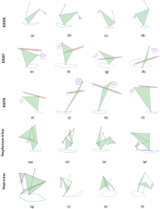
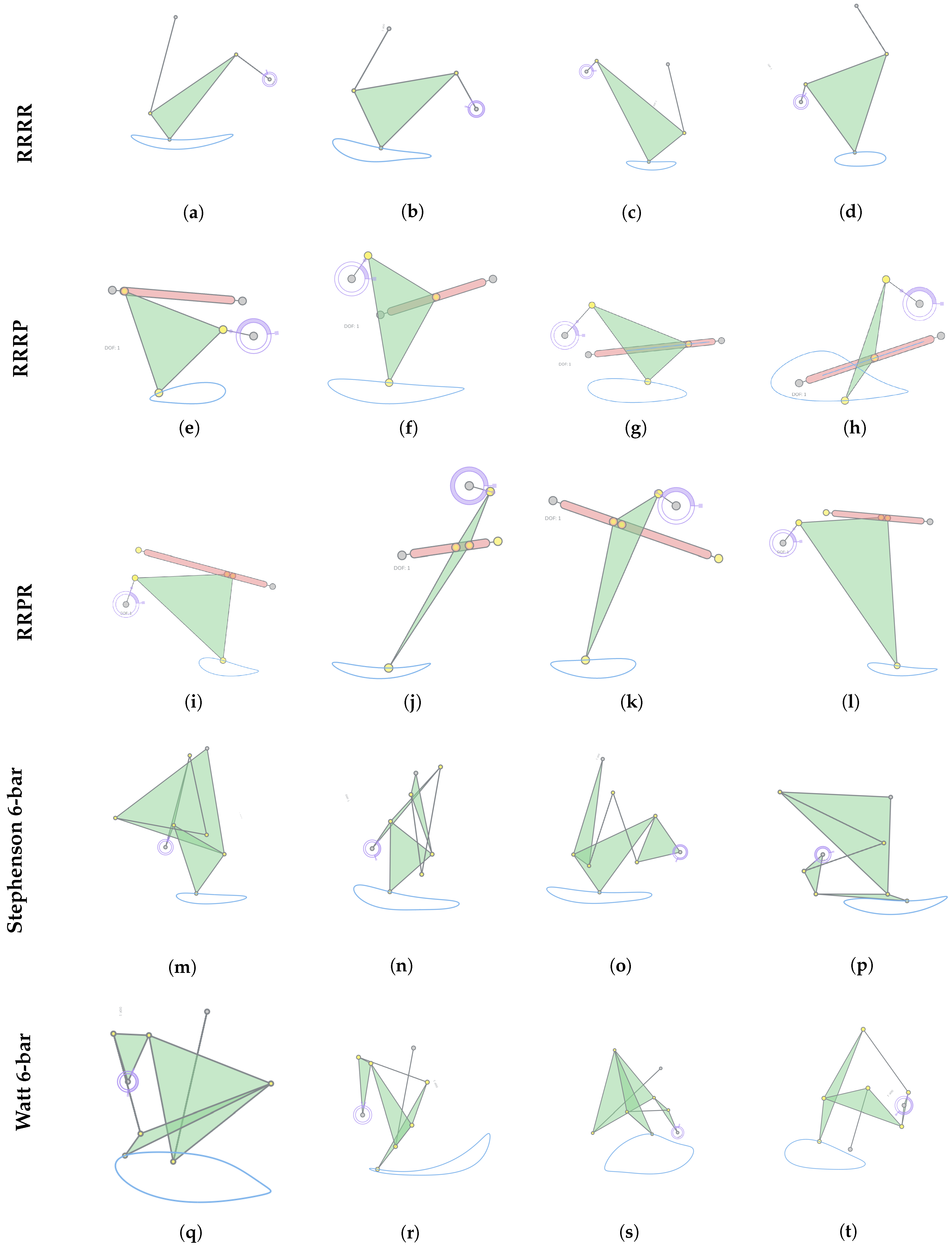
Dataset generation was performed on Stony Brook University’s SeaWulf computing cluster. We simulated approximately $4\times {10}^6$ mechanisms for each of 25 mechanism subtypes (i.e., on the order of ${10}^8$ total candidates). Among all simulated candidates, 23,250 mechanisms satisfied the proposed geometric criteria and were retained in the dataset. Figure 9 shows representative examples from the resulting dataset, and Table 1 shows the number of mechanisms generated per type, and aggregate statistics for each family. (For six-bar families, different variants define the coupler point on different links. The corresponding kinematic structures are publicly provided in the BSIdict at [21]). The filtered dataset of 23,250 mechanisms is publicly available [33] and contains data of mechanism type and initial joint coordinates.

Figure 9. Selected walking mechanisms from the filtered dataset rendered using the MotionGen (2026) software. Subfigures (a–d) are 4-bar RRRR mechanisms, (e–h) are 4-bar RRRP mechanisms, (i–l) are 4-bar RRPR mechanisms, (m–p) are Stephenson 6-bars, and (q–t) are Watt 6-bars.

Table 1. Number of Generated Mechanisms in Filtered Dataset and their Acceptance Rates.

Mechanism Type	Count	Mechanism Acceptance Rate (%)
Total (4-bar + 6-bar)	23,250	0.02325000
4-bar Mechanisms	12,783	0.07989375
RRRR	3926	0.09815000
RRRP	8219	0.20547500
RRPR	621	0.01552500
PRPR	17	0.00042500
6-bar Mechanisms	10,467	0.01246071
Stephenson (all variants)	3781	0.00859318
Watt (all variants)	6686	0.01671500

3.2. Optimization Results

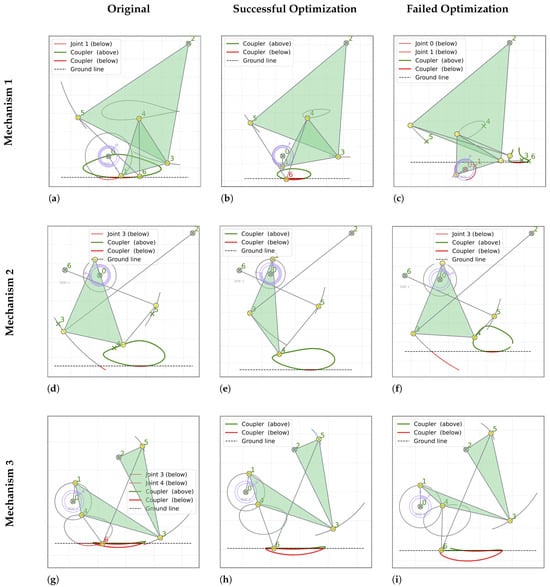
A subset of the retained mechanisms still exhibits geometric violations that prevent physical walking, most commonly due to non-foot joints intersecting the estimated ground line. We therefore evaluate the proposed fine-tuning procedure (Figure 3) for correcting these near-feasible candidates using the custom objective defined in Section 2.3. Three representative near-walking mechanisms are selected, and ten independent optimization trials are performed for each. Table 2 reports the corresponding success rates, and Figure 10 compares the trajectories before and after optimization.

Table 2. Optimization Results for Selected Mechanisms.

Mechanism Type	Success	Fail
Example Mechanism 1	8	2
Example Mechanism 2	6	4
Example Mechanism 3	6	4

Figure 10. Optimization results for three example mechanisms. Each row corresponds to results for one example mechanism. Each column shows a stage of optimization: the original mechanism, asuccessful optimization, and afailed attempt. One representative success and failure are shown per mechanism. (a,d,g) are the original three mechanisms, (b,e,h) are the succesfully optimized mechanism versions, and (c,f,i) are the failed optimization runs. Note the common features in the failed optimization trials shown—most failed runs were because the coupler curvesremain under the ground line (c,f) or because the curve became open (c,f,i).

Across the evaluated cases, optimization success rates ranged from 30–90%. Failures were primarily associated with trajectories becoming effectively open (loss of closure) or with persistent ground intersections of non-foot joint trajectories. Consistent with intuition, candidates that were closer to feasibility at initialization typically required smaller adjustments and achieved higher success rates. Since differential evolution is stochastic, repeated runs can yield different outcomes; we therefore report results over multiple trials for each mechanism (Table 2).

Table 3 shows the detailed error components for the three representative mechanisms for their original, successful and failed optimization runs. Successful optimization eliminates or significantly reduces error components: ground violation penalty L is reduced to zero in successful cases, while failed optimizations show L values one-to-two orders of magnitude higher, indicating persistent ground intersections and the optimizer getting stuck in local minima. Intersection penalty I and closure penalty C remain zero across all cases, confirming these hard constraints were maintained consistently. Walking penalty W is presented in some original mechanisms but is eliminated during successful optimization. The dramatic reduction in total error (up to 17 orders of magnitude for Mechanism 1) demonstrates the effectiveness of the penalty-based optimization approach.

Table 3. Optimization Error Component Analysis for Representative Mechanisms.

Mechanism	State	I	W	L	C	Total Error
Mechanism 1	Original	$2.00\times {10}^8$	$1.00\times {10}^4$	$5.49\times {10}^{16}$	0.0	$5.49\times {10}^{16}$
	Success	0.0	0.0	0.0	0.0	0.0
	Fail	0.0	0.0	$8.88\times {10}^{18}$	0.0	$8.88\times {10}^{18}$
Mechanism 2	Original	0.0	$1.00\times {10}^4$	$3.59\times {10}^{16}$	0.0	$3.59\times {10}^{16}$
	Success	0.0	$1.00\times {10}^4$	0.0	0.0	$1.00\times {10}^4$
	Fail	0.0	0.0	$1.95\times {10}^{18}$	0.0	$1.95\times {10}^{18}$
Mechanism 3	Original	0.0	0.0	$6.05\times {10}^{17}$	0.0	$6.05\times {10}^{17}$
	Success	0.0	0.0	0.0	0.0	0.0
	Fail	0.0	0.0	$1.00\times {10}^{18}$	0.0	$1.00\times {10}^{18}$

Table 4 shows detailed improvement percentages for all error components from Table 3. Analysis of successful versus failed optimization runs reveals a clear trend: mechanisms with lower initial ground-violation penalties (L) exhibit higher convergence rates, whereas candidates with large initial L values are more likely to fail.

Table 4. Optimization Improvement Metrics for All Error Components.

Case	I (Intersection)		W (Walking)		L (Ground)		E (Total)
	Initial	Final	Initial	Final	Initial	Final	Initial	Final
Mech 1 Success	$2.00\times {10}^8$	0.0	$1.00\times {10}^4$	0.0	$5.49\times {10}^{16}$	0.0	$5.49\times {10}^{16}$	0.0
Reduction	100%		100%		100%		100%
Mech 1 Fail	$2.00\times {10}^8$	0.0	$1.00\times {10}^4$	0.0	$5.49\times {10}^{16}$	$8.88\times {10}^{18}$	$5.49\times {10}^{16}$	$8.88\times {10}^{18}$
Reduction	100%		100%		−16,172%		−16,172%
Mech 2 Success	0.0	0.0	$1.00\times {10}^4$	$1.00\times {10}^4$	$3.59\times {10}^{16}$	0.0	$3.59\times {10}^{16}$	$1.00\times {10}^4$
Reduction	—		0%		100%		>99.9999%
Mech 2 Fail	0.0	0.0	$1.00\times {10}^4$	0.0	$3.59\times {10}^{16}$	$1.95\times {10}^{18}$	$3.59\times {10}^{16}$	$1.95\times {10}^{18}$
Reduction	—		100%		$-5331\%$		$-5331\%$
Mech 3 Success	0.0	0.0	0.0	0.0	$6.05\times {10}^{17}$	0.0	$6.05\times {10}^{17}$	0.0
Reduction	—		—		100%		100%
Mech 3 Fail	0.0	0.0	0.0	0.0	$6.05\times {10}^{17}$	$1.00\times {10}^{18}$	$6.05\times {10}^{17}$	$1.00\times {10}^{18}$
Reduction	—		—		$-65\%$		$-65\%$

These observations suggest that the proposed differential evolution framework is effective as a refinement tool for mechanisms that are already close to geometric feasibility. Rather than transforming highly infeasible candidates, the optimizer reliably corrects minor violations while preserving closure and intersection constraints. This behavior aligns with the intended design of the filtering–optimization pipeline.

3.3. Optimization Robustness Evaluation

To evaluate robustness beyond the three illustrative examples in Table 2, the optimization procedure was applied to a total of 10 near-walking mechanisms, including the three representative examples previously presented and seven additional cases randomly selected from the filtered dataset.

The mean final error across all 10 cases was $\mu =8.85\times {10}^{17}$, with standard deviation $\sigma =2.68\times {10}^{18}$. These statistics are summarized in Table 5 Considering only converged cases, the success rate was 50%, increasing to 70% when including partially improved solutions.

Table 5. Statistical summary of optimization performance over 10 additional near-walking mechanisms.

Metric	Value
Mean Initial Total Error	$1.62\times {10}^{18}$
Mean Final Total Error	$8.85\times {10}^{17}$
Standard Deviation (Final Error)	$2.68\times {10}^{18}$
Full Convergence Rate	50%
Improvement Rate (Final < Initial)	70%

Among these 10 cases:

• 5 converged to zero total error,
• 2 achieved substantial reduction in geometric error but retained minor walk penalties,
• 3 did not converge to feasible closed configurations.

Across the ten evaluated mechanisms, five converged to zero total error, while two exhibited substantial error reduction but did not fully eliminate ground violations. Three cases diverged due to loss of trajectory closure. The mean final error therefore reflects a mixture of successful and failed trials, inflating the average despite complete convergence in half of the cases. When considering only successful runs, the final error is identically zero.

3.4. Comparative Analysis with Classic Walking Mechanisms

In this section, we compare a representative mechanism discovered through our geometric filtering pipeline with the classic Klann linkage (Stephenson III configuration). Figure 11 presents a side-by-side comparison of (left) the Klann linkage, (middle) a geometrically feasible Watt I mechanism from our dataset exhibiting similar walking characteristics, and (right) a modified version of the generated mechanism adjusted for manufacturability using straight links.

Figure 11. Comparison of classic and generated walking mechanisms. (a): Klann linkage (Stephenson III). (b): geometrically feasible Watt I mechanism discovered through the proposed filtering pipeline. (c): refined version of the generated mechanism with straight links for manufacturability.

All these three mechanisms produce feasible walking trajectories. However, mechanism in Figure 11b,c require only two ground joints, whereas the Klann linkage in Figure 11a needs three. This reduction may simplify structural support and anchoring requirements in practical implementations.

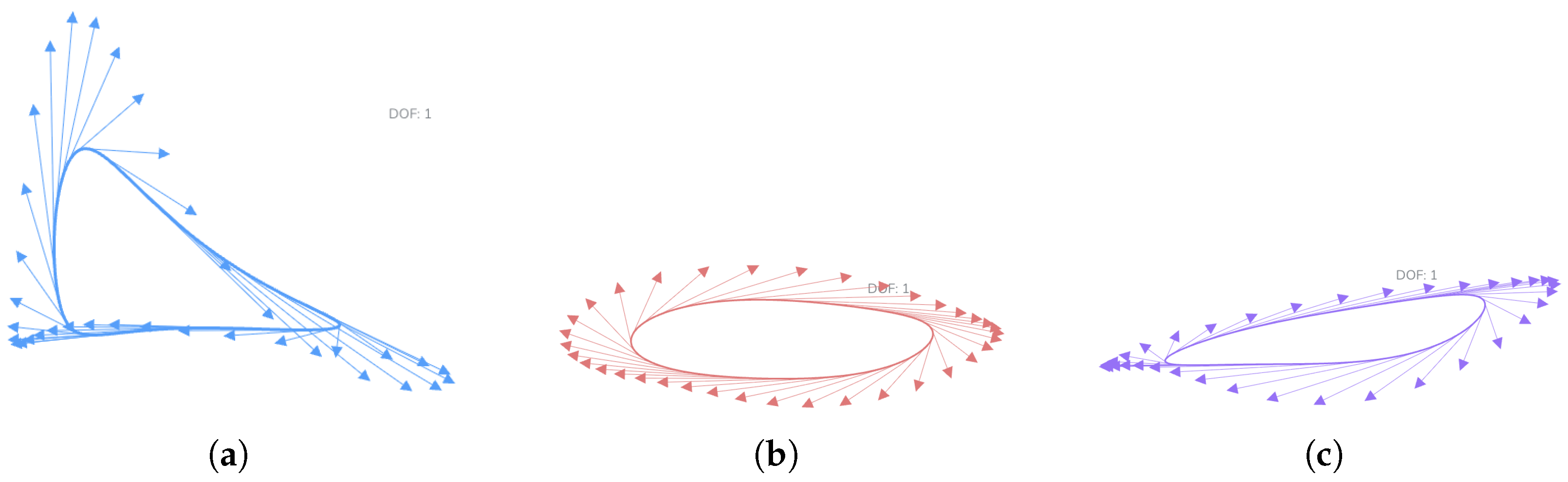
To further examine kinematic behavior, Figure 12 compares the foot trajectories and instantaneous velocity fields of the Klann linkage, the generated mechanism, and the refined generated mechanism. The resulting coupler curves exhibit comparable stride geometries and ground-contact behavior. Additionally, the velocity vectors of the generated mechanism indicate smoother kinematic transitions under the applied geometric constraints. This is especially seen throughout the stance phase, suggesting improved kinematic continuity under the geometric constraints enforced during filtering and optimization.

Figure 12. Foot trajectory and velocity comparison between the three mechanisms. (a): The foot trajectory of the existing Klann Linkage. (b): Foot trajectory of the discovered Watt mechanism. (c): Foot trajectory of the modified Watt mechanism. Comparable stride envelopes are observed in (b,c). The generated mechanism exhibits smoother velocity direction transitions during stance.

The rightmost configuration in Figure 11 illustrates a manually refined variant of the generated mechanism in which triangular links are replaced with straight members to reflect improved manufacturability. This modification was performed to demonstrate that geometrically feasible walking behavior can be preserved under structural simplification. While the present optimization framework does not explicitly enforce manufacturability constraints, this example suggests that additional objective terms or geometric penalties could be incorporated in future work to systematically account for fabrication-oriented design considerations.

While this comparison does not constitute a full dynamic or energetic evaluation, it demonstrates that the proposed geometric synthesis framework is capable of producing structurally distinct walking mechanisms with kinematic behavior comparable to established designs, and that these mechanisms can be further adapted to practical engineering considerations.

4. Conclusions and Future Outlook

This paper presented a design-criteria-driven kinematic synthesis pipeline for planar 1-DOF walking mechanisms within selected 4-bar and 6-bar mechanism families. The proposed workflow combines large-scale simulation, automated geometric filtering, and optimization-based refinement to construct a curated dataset of feasible walking candidates and to improve near-feasible designs.

Using the proposed filters, we evaluated approximately 100,000,000 mechanisms across 25 subtypes and obtained a dataset of 23,250 walking mechanisms. Only approximately 0.024% of the sampled designs satisfied the walking criteria, indicating that feasible walking behavior is rare under naive random sampling and that multi-criterion feasibility constraints significantly restrict the design space. To increase yield beyond filtering alone, we introduced a custom, design-driven objective for refinement of near-feasible candidates. Across the tested cases, the optimization success rate ranged from 30–90% (Table 2), demonstrating that targeted refinement can substantially improve feasibility relative to pure sampling and filtering.

Looking ahead, the central idea of treating application performance as computable geometric/kinematic criteria suggests a general path toward task-specific dataset construction and synthesis in mechanism design. Future work will focus on extending the approach to additional mechanism families and applications, improving sampling strategies to reduce computational cost, and integrating learning-based models to guide search toward high-feasibility regions of the design space while preserving strict feasibility checks via simulation.

Additionally, although the present work focuses on geometric feasibility and large-scale mechanism generation, the resulting database of over 23,000 walking-feasible designs presents an opportunity for future statistical analysis. Pattern extraction techniques could be applied to investigate correlations between link-length ratios, joint distributions, and qualitative walking characteristics. Such analysis may enable the derivation of higher-level structural design principles beyond the geometric criteria imposed in this study.

4.1. Limitations

A primary limitation is computational cost. In this study, only 0.024% of the 100 million evaluated mechanisms passed the filters, implying that brute-force dataset generation can require large-scale computation for narrow or strict criteria. On average, evaluating and filtering 4 million mechanisms for a single subtype required approximately 5–6 h on Stony Brook University’s SeaWulf computing resources. Running the same workload on typical personal hardware would be substantially slower, which may limit practicality for users without access to high-performance computing or for problems with similarly low feasibility rates.

A second limitation is that the filtering criteria are application-dependent. While the pipeline is general, each new robotics task requires the specification of appropriate feasibility and performance criteria (e.g., collision avoidance, workspace constraints, payload clearance, or timing requirements). Designing such criteria may require domain expertise and iterative validation to ensure that the filters reflect the true functional requirements rather than an overly restrictive proxy. Nevertheless, once formulated, these criteria can be evaluated systematically at scale within the same simulation–filter–refine framework.

4.2. Integration with Physical Design

While this work focuses on geometric feasibility, future work could potentially explore physical implementation. Generated mechanisms could be coupled with: (1) dynamic analysis via physics-based linkage simulation to evaluate stability, contact forces, and torque, (2) control synthesis for actuation timing, (3) morphological optimization for leg compliance and energy efficiency, and (4) manufacturing constraints (link thickness, joint clearances). Our filtered dataset provides a high-quality starting point for these downstream design stages. Additionally, transmission angles are not explicitly constrained in the present study. Incorporating transmission-angle bounds represents another important extension for future physically realizable designs.

References

- Purwar, A. MotionGen. 2026. Available online: http://www.motiongen.io (accessed on 21 January 2026).
- Lyu, Z.; Purwar, A.; Liao, W. A Unified Real-Time Motion Generation Algorithm for Approximate Position Analysis of Planar N-Bar Mechanisms. ASME J. Mech. Des. 2023, 146, 063302. [Google Scholar] [CrossRef] [Scilit]
- Garbuz, M.; Klimina, L.; Samsonov, V. Wind driven plantigrade machine capable of moving against the flow. Appl. Math. Model. 2022, 110, 17–27. [Google Scholar] [CrossRef] [Scilit]
- Klann, J.C. Walking Device. US6260862B1, 11 February 1998. [Google Scholar]
- Nansai, S.; Elara, M.R.; Iwase, M. Dynamic Analysis and Modeling of Jansen Mechanism. Procedia Eng. 2013, 64, 1562–1571. [Google Scholar] [CrossRef] [Scilit]
- Nansai, S.; Rojas, N.; Elara, M.R.; Sosa, R.; Iwase, M. On a Jansen leg with multiple gait patterns for reconfigurable walking platforms. Adv. Mech. Eng. 2015, 7, 1687814015573824. [Google Scholar] [CrossRef] [Scilit]
- Norton, R. Design of Machinery: An Introduction To The Synthesis and Analysis of Mechanisms and Machines, 5th ed.; McGraw Hill: Columbus, OH, USA, 2011. [Google Scholar]
- Erdman, A.G.; Sandor, G.N. Mechanism Design: Analysis and Synthesis, 2nd ed.; Prentice-Hall: Englewood Cliffs, NJ, USA, 1991; Volume 1. [Google Scholar]
- Ge, Q.; Purwar, A.; Zhao, P.; Deshpande, S. A Task-Driven Approach to Unified Synthesis of Planar Four-Bar Linkages Using Algebraic Fitting of a Pencil of G-Manifolds. ASME J. Comput. Inf. Sci. Eng. 2017, 17, 031011. [Google Scholar] [CrossRef] [Scilit]
- Galan-Marin, G.; Alonso, F.J.; Del Castillo, J.M. Shape optimization for path synthesis of crank-rocker mechanisms using a wavelet-based neural network. Mech. Mach. Theory 2009, 44, 1132–1143. [Google Scholar] [CrossRef] [Scilit]
- Nurizada, A.; Purwar, A. An Invariant Representation of Coupler Curves Using a Variational AutoEncoder: Application to Path Synthesis of Four-Bar Mechanisms. ASME J. Comput. Inf. Sci. Eng. 2023, 24, 011008. [Google Scholar] [CrossRef] [Scilit]
- Nobari, A.; Srivastava, A.; Gutfreund, D.; Xu, K.; Ahmed, F. LInK: Learning Joint Representations of Design and Performance Spaces through Contrastive Learning for Mechanism Synthesis. arXiv 2024, arXiv:2405.20592. [Google Scholar] [CrossRef] [Scilit]
- Nobari, A.H.; Srivastava, A.; Gutfreund, D.; Ahmed, F. LINKS: A Dataset of a Hundred Million Planar Linkage Mechanisms for Data-Driven Kinematic Design. In Proceedings of the Volume 3A: 48th Design Automation Conference (DAC); American Society of Mechanical Engineers: New York, NY, USA, 2022. [Google Scholar] [CrossRef] [Scilit]
- Nurizada, A.; Dhaipule, R.; Lyu, Z.; Purwar, A. A Dataset of 3M Single-DOF Planar 4-, 6-, and 8-Bar Linkage Mechanisms With Open and Closed Coupler Curves for Machine Learning-Driven Path Synthesis. ASME J. Mech. Des. 2024, 147, 041702. [Google Scholar] [CrossRef] [Scilit]
- Lyu, Z.; Purwar, A. Deep Learning Conceptual Design of Sit-to-Stand Parallel Motion Six-Bar Mechanisms. ASME J. Mech. Des. 2024, 147, 013306. [Google Scholar] [CrossRef] [Scilit]
- Nobari, A.H.; Chen, W.; Ahmed, F. Range-Constrained Generative Adversarial Network: Design Synthesis Under Constraints Using Conditional Generative Adversarial Networks. J. Mech. Des. 2021, 144, 021708. [Google Scholar] [CrossRef] [Scilit]
- Vermeer, K.; Kuppens, R.; Herder, J. Kinematic Synthesis Using Reinforcement Learning. In Proceedings of the Volume 2A: 44th Design Automation Conference; American Society of Mechanical Engineers: New York, NY, USA, 2018. [Google Scholar] [CrossRef] [Scilit]
- Fogelson, M.B.; Tucker, C.; Cagan, J. GCP-HOLO: Generating High-Order Linkage Graphs for Path Synthesis. J. Mech. Des. 2023, 145, 073303. [Google Scholar] [CrossRef] [Scilit]
- Bolanos, D.; Ataei, M.; Jayaraman, P. MechaFormer: Sequence Learning for Kinematic Mechanism Design Automation. arXiv 2025, arXiv:2508.09005. [Google Scholar] [CrossRef] [Scilit]
- Kapsalyamov, A.; Hussain, S.; Brown, N.A.; Goecke, R.; Hayat, M.; Jamwal, P.K. Synthesis of a six-bar mechanism for generating knee and ankle motion trajectories using deep generative neural network. Eng. Appl. Artif. Intell. 2023, 117, 105500. [Google Scholar] [CrossRef] [Scilit]
- Purwar Lab. Four, Six and Eight-Bar Mechanisms With Curves. 2025. Available online: https://www.kaggle.com/datasets/purwarlab/four-six-and-eight-bar-mechanisms-with-curves (accessed on 21 January 2026).
- Storn, R.; Price, K. Differential Evolution—A Simple and Efficient Heuristic for Global Optimization over Continuous Spaces. J. Glob. Optim. 1997, 11, 341–359. [Google Scholar] [CrossRef] [Scilit]
- Chen, C.H. Application of Multiple Deep Neural Networks to Multi-Solution Synthesis of Linkage Mechanisms. Machines 2023, 11, 1018. [Google Scholar] [CrossRef] [Scilit]
- Zhang, Y.; Arakelian, V. Design and Synthesis of Single-Actuator Walking Robots via Coupling of Linkages. Front. Mech. Eng. 2021, 6, 609340. [Google Scholar] [CrossRef] [Scilit]
- Amine, S.; Prasad, B.; Saber, A.; Mokhiamar, O.; Gazo-Hanna, E. Design and Analysis of a Planar Six-Bar Crank-Driven Leg Mechanism for Walking Robots. Appl. Sci. 2024, 14, 8919. [Google Scholar] [CrossRef] [Scilit]
- Shigley, J.E. The Mechanics of Walking Vehicles: A Feasibility Study. Technical Report AD419858, U.S. Army Ordnance Corps/U.S. Army Tank Automotive Command, 1960. Archived by the U.S. Department of Defense Technical Information Center. Available online: https://apps.dtic.mil/sti/tr/pdf/AD0419858.pdf (accessed on 13 January 2026).
- Gogate, G.R.; Matekar, S.B. Optimum synthesis of motion generating four-bar mechanisms using alternate error functions. Mech. Mach. Theory 2012, 54, 41–61. [Google Scholar] [CrossRef] [Scilit]
- Gao, W.; Liu, S. Improved artificial bee colony algorithm for global optimization. Inf. Process. Lett. 2011, 111, 871–882. [Google Scholar] [CrossRef] [Scilit]
- Deb, K. Multi-Objective Optimization Using Evolutionary Algorithms; John Wiley & Sons: Chichester, UK, 2001. [Google Scholar]
- Zhang, R.; Ning, M.; Wang, Y.; Yang, J. Design and Dimension Optimization of Rigid–Soft Hand Function Rehabilitation Robots. Machines 2025, 13, 311. [Google Scholar] [CrossRef] [Scilit]
- Cabrera, J.; Ortiz, A.; Nadal, F.; Castillo, J. An evolutionary algorithm for path synthesis of mechanisms. Mech. Mach. Theory 2011, 46, 127–141. [Google Scholar] [CrossRef] [Scilit]
- Liu, X.; Ding, J.; Wang, C. Design Framework for Motion Generation of Planar Four-Bar Linkage Considering Clearance Joints and Dynamics Performance. Machines 2022, 10, 136. [Google Scholar] [CrossRef] [Scilit]
- Purwar Lab. A Dataset of Planar 1-DOF Walking Linkages. 2025. Available online: https://www.kaggle.com/datasets/purwarlab/walking-mechanisms (accessed on 21 January 2026).
Disclaimer/Publisher’s Note: The statements, opinions and data contained in all publications are solely those of the individual author(s) and contributor(s) and not of MDPI and/or the editor(s). MDPI and/or the editor(s) disclaim responsibility for any injury to people or property resulting from any ideas, methods, instructions or products referred to in the content. |
© 2026 by the authors. Licensee MDPI, Basel, Switzerland. This article is an open access article distributed under the terms and conditions of the Creative Commons Attribution (CC BY) license.