


Abstract
Semiconductor manufacturing equipment such as vacuum pumps, wafer handling mechanisms, etching machines, and deposition systems operates for a long time under high vacuum, high temperature, strong electromagnetic, and high-precision continuous production environments. Its reliability is directly related to the yield and stability of the production line. During equipment operation, the fault signals are often weak, the noise is strong, and the working conditions are variable, so traditional methods are difficult to achieve high-precision recognition. To solve this problem, this paper proposes a fault diagnosis and health monitoring method for semiconductor manufacturing equipment based on deep learning and subspace transfer. Firstly, considering the cyclostationary characteristics of the operating signals of key equipment, the cyclic spectral analysis technology is used to obtain the cyclic spectral coherence map, which effectively reveals the feature differences under different health states. Then, a deep fault diagnosis model based on the convolutional neural network (CNN) is constructed to extract deep feature representations. Furthermore, the subspace transfer learning technology is introduced, and group normalization and correlation alignment unsupervised adaptation layers are designed to achieve automatic alignment and enhancement of the statistical characteristics of deep features between the source domain and the target domain, which effectively improves the generalization and adaptability of the model. Finally, simulation experiments based on the public bearing dataset verify that the proposed method has strong feature representation ability and high classification accuracy under different working conditions and different loads. Because the key components and experimental scenarios of semiconductor manufacturing equipment have similar signal characteristics, this method can be directly transferred to the early fault diagnosis and health monitoring of semiconductor production line equipment, which has important engineering application value.
1. Introduction
The semiconductor industry is the core industry supporting the development of modern electronic information technology, and semiconductor manufacturing equipment, as its fundamental sup-porting link, plays a decisive role in the yield, manufacturing efficiency, and process stability of the production line. Typical semiconductor manufacturing equipment includes vacuum pumps, etchers, chemical vapor deposition equipment, lithography machines, wafer handling robotic arms, etc. These devices generally operate in harsh environments such as high vacuum, high temperature, strong plasma, or high-precision positioning. Any minor failure of key components may cause the shutdown of the entire production line, resulting in huge eco-nomic losses. According to industrial statistics, the loss caused by the shutdown of a high-end wafer production line can reach tens of thousands of US dollars per hour. Therefore, real-time monitoring of equipment operating status and early fault diagnosis are particularly important in the semiconductor industry.
However, due to the complex and variable working conditions of semiconductor equipment and strong noise interference in signals, the fault signals of equipment during operation are often very weak, and the data distribution differences are significant, resulting in the fact that traditional di-agnostic methods based on manual features or fixed models are difficult to achieve stable and accurate results [1,2]. In particular, after long-term service of equipment, factors such as load variation, environ-mental drift, and component aging further intensify the distribution shift between the source domain and the target domain, leading to a significant de-cline in diagnostic accuracy and generalization ability [3,4]. On 18 October 2023, a serious safety accident occurred in a phase I elevator of the Fo Cheng Shang Du Project in Mile City, Honghe Prefecture, Yunnan Province, due to the fatigue failure of the counterweight sheave rolling bearing [5]. Therefore, for the rolling bearing failures that may occur during the operation of semiconductor manufacturing equipment such as lithography machines, carrying out research on equipment condition monitoring and fault diagnosis, detecting, locating, diagnosing, and predicting possible equipment faults to “pre-vent problems before they occur” is of great practical significance for ensuring the safe and stable operation of the equipment, reducing economic losses and operating costs, and avoiding major accidents.
The semiconductor manufacturing equipment fault prognostics and health management (PHM) technology centered on prediction has also received increasing attention and application domestically and abroad in recent years. In particular, the rise in deep neural networks and transfer learning technologies has provided strong technical support for intelligent diagnosis and condition monitoring of equipment rolling bearings. The advantage of deep neural networks lies in “feature extraction,” but their performance usually depends on a large amount of training data, and at the same time, re-quires that the testing and training data satisfy the assumption of independent and identical distribution. Therefore, they are not suitable for fields with small training data, scene changes, or task variations. Transfer learning, as a new machine learning paradigm, can extract knowledge from one or more related domains to help improve learning performance in the target domain. It not only reduces the requirement for data volume but also relaxes the assumption of independent and identical distribution, providing a new solution to the above deficiencies [6].
In the field of fault diagnosis, some scholars have adopted time–frequency domain features and transfer component analysis (TCA) [7], singular value decomposition and TrAdaBoost transfer algorithms [8], and neural network-assisted classifier training [9] to carry out some studies on transfer learning-based intelligent diagnosis methods. In addition, combining deep neural networks and transfer learning technologies to study deep transfer learning methods based on feature representation has achieved preliminary exploration and application in mechanical fault diagnosis under variable speed and variable load conditions [10]. Jia et al. [11] proposed a rolling bearing fault diagnosis method based on deep transfer learning and adaptive weighting, using the idea of transfer learning to design a weighted domain discriminator to increase the domain similarity of shared health state samples between the target and source domains, solving the problem that additional fault state samples in the target domain affect the diagnostic accuracy. Yang et al. [12] proposed a mechanical fault diagnosis method based on multi-source deep transfer learning, which integrates fault feature in-formation from multiple source domains to extract domain-invariant features, avoiding the problem of negative transfer and improving the generalization ability of the model. Shao et al. [13] directly used the Alex Net model pre-trained on ImageNet, fine-tuned the higher layers of the network using time–frequency maps, and improved bearing diagnostic accuracy under small sample conditions. Han [14] proposed a deep adversarial transfer network diagnosis model that effectively trains and con-structs diagnostic networks using the gradient re-versal layer and stochastic gradient descent method, showing good classification accuracy and generalization ability on transfer tasks with different loads. Chen et al. [15] proposed an enhanced transfer convolutional neural network (ETCNN) to improve the diagnostic accuracy and generalization ability of mechanical equipment under variable working conditions, addressing the problem of poor adaptability of training models to real industrial environments. However, under normal working conditions, equipment failures in industrial robots do not occur frequently, and thus the generated fault data are insufficient, leading to a small-sample problem [2,16,17]. In recent years, interpretable sparse time–frequency representation methods have attracted increasing attention in mechanical fault diagnosis, such as the Matching Pursuit Network (MPN) [18].
Although the physical mechanisms of rolling bearing failures, such as fatigue spalling, and the vibration signal generation models characterized by periodic impulsive excitation are generally applicable across rotating machinery, the extreme operating conditions of semiconductor manufacturing equipment pose unique challenges for fault diagnosis. Conventional bearing diagnosis in gearboxes typically deals with vibration signals with relatively clear structural transmission paths and higher signal-to-noise ratios. In contrast, bearing signals in semiconductor equipment, such as vacuum pumps, are severely contaminated by high vacuum environments, elevated temperatures, and strong process-induced noise, resulting in significantly weaker fault signatures, more complex modulation characteristics, and stronger non-stationary behavior. Consequently, diagnostic models trained directly on data from traditional scenarios often fail when applied to such conditions.
To address the difficulty of extracting weak fault signatures under strong noise and variable operating conditions, this study develops a deep learning framework combining cyclostationary spectral analysis and subspace transfer. The proposed method enhances early bearing fault feature extraction and enables robust diagnosis across different operating conditions, thereby satisfying the stringent demands for high reliability and adaptability in monitoring semiconductor manufacturing equipment. In data preprocessing, considering that the vibration response of rotating machinery shows cyclostationary modulated signals when faults occur, the cyclic spectral analysis technique is adopted to obtain the two-dimensional cyclic spectral coherence mapping to reveal the hidden fault modes in vibration signals. In addition, to enhance the feature learning and adaptive capability of convolutional neural net-works, based on the subspace transfer learning strategy, two unsupervised adaptation layers are constructed and embedded into the traditional CNN. The CNN is used to map source and target domain data into a high-dimensional feature subspace. Based on statistical feature transformation, group normalization adaptation layers and correlation alignment adaptation layers are constructed to align the first-order and second-order statistical features between the source and target domains, thereby alleviating the mismatch problem caused by data distribution differences between the source and target domains and improving the generalization performance of the diagnostic network. Finally, the effectiveness of the algorithm is verified using the public MFPT bearing fault dataset. The results show that the proposed CNN (GN-CORAL) method improves CNN’s feature extraction and classification capability under different diagnostic tasks from the perspectives of feature preprocessing and network learning, providing an effective solution for such problems.
2. Convolutional Neural Networks (CNN)
The CNN is a kind of multi-layer deep neural network, which can combine low-level features to form more abstract high-level representations [19]. CNN has four basic characteristics, namely local feature extraction, nonlinear mapping, weight sharing, and feature pooling. Compared with a fully connected network, CNN can significantly reduce the number of trainable parameters without losing expressive power, thus promoting efficient training. A typical CNN structure generally includes convolutional layers, activation functions, pooling layers, and fully connected layers.
2.1. Convolutional Layer
The name of the Convolutional Neural Network originates from the “convolution” operation, which is characterized by linearity and translation invariance. The main purpose of the convolution operation is to extract local features by performing weighted summation on the input data. In performing convolution, multiple convolution kernels are first constructed, and the neurons in each kernel are connected to a small local region of the input feature map to perform convolution operations. Since the weight-sharing strategy is adopted, the same convolution kernel is used to perform convolution operations on different regions of the same image to obtain the features of each region. By constructing multiple convolution filters, multiple different feature outputs can be generated, and the output features are also called feature maps.
For each input and convolution kernel , the output feature is calculated as follows:
where denotes the convolution operation, b is the bias term, k is the convolution matrix, and y is the feature map output.
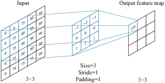
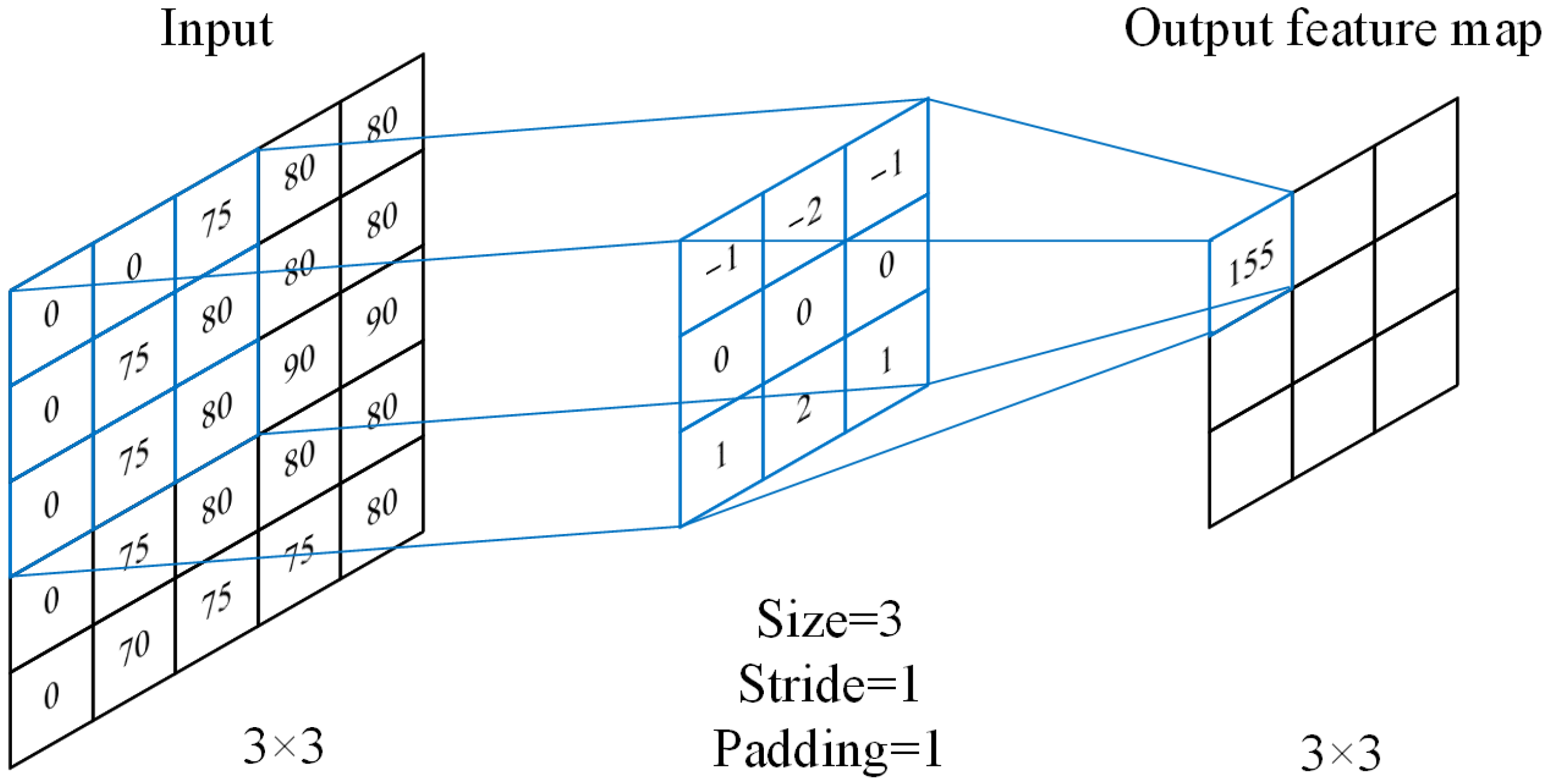
During the convolution operation, several core parameters affect the output of the feature map, including kernel size, stride, and zero padding. As shown in Figure 1, the size of the convolution kernel usually determines the dimension of the output feature and the fineness of feature extraction. In general, the kernel size must be greater than 1 to effectively expand the receptive field. Under the same receptive field, the smaller the kernel size, the fewer parameters and computations are required. When the kernel size is even, symmetric zero pad-ding cannot guarantee that the output feature map size equals the input size, so an odd kernel size is usually used. The stride indicates the number of pixels that the convolution kernel moves on the input image each time. The larger the stride, the smaller the generated feature map. When the stride equals 1, the kernel moves one pixel each time. Zero padding fills the borders of the input matrix with zeros, which can control the size of the feature map and ensure the same dimension as the input.
Figure 1.
Convolution operation on the input image.
2.2. Activation Function
After the convolution operation, the neural network needs to introduce an activation function to perform feature mapping. Usually, nonlinear activation functions are introduced so that the neural network can learn complex function representations. The most widely used activation functions in the early stages were Sigmoid and Tanh functions. The Sigmoid function, also known as the logistic function, maps any input to an output in the range (0, 1). When the function value approaches 0 or 1, the curve becomes very flat, so the gradient in these regions is close to 0. These neurons become saturated neurons. During backpropagation, the gradient of saturated neurons becomes very small, causing their weights to fail to update, and the weights of other neurons connected to them also update slowly. This phenomenon is called the vanishing gradient problem. The Tanh function compresses a real number into the range (−1, 1). Similar to Sigmoid, when the function value approaches −1 or 1, the gradient also approaches 0, so Tanh also suffers from the vanishing gradient problem.
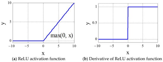
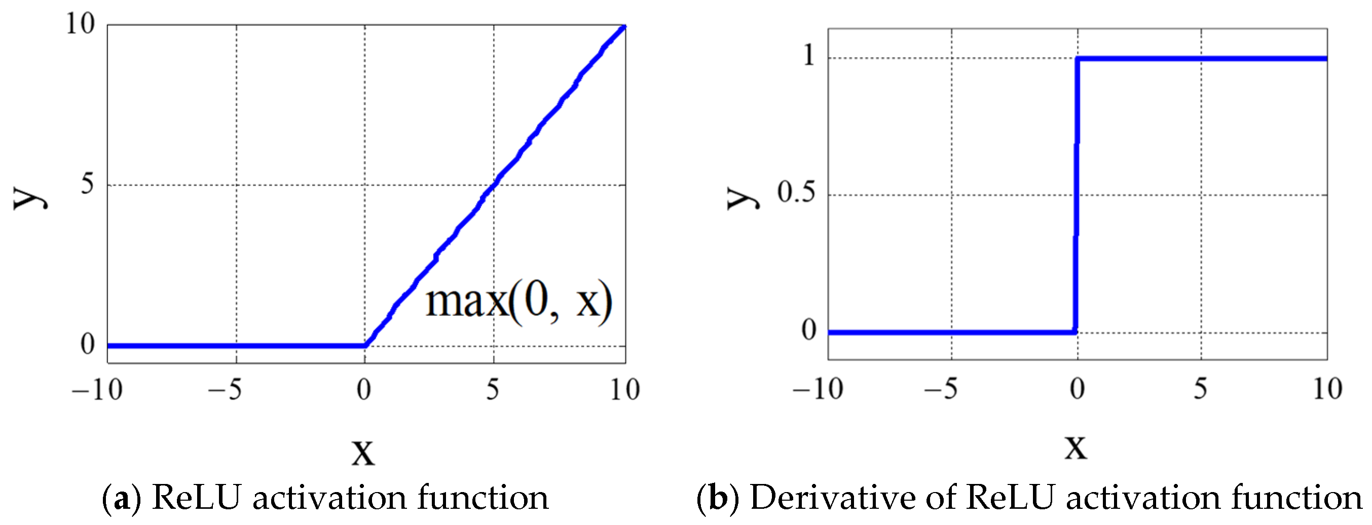
To solve the vanishing gradient problem, the Rectified Linear Unit (ReLU) was proposed to replace Tanh and Sigmoid as the activation function [20]. ReLU not only alleviates the vanishing gradient problem but also accelerates the convergence of the network. The curve of ReLU and its derivative are shown in Figure 2.
Figure 2.
ReLU activation function properties.
The ReLU activation function performs a half-rectified on the input. Its expression and derivative are as follows:
When the input , the output is 0, when x > 0, the output equals x. Since the derivative is nonzero and linear for positive inputs, ReLU does not saturate and can alleviate the vanishing gradient problem. In addition, when training a deep neural model, since the ReLU function maps half of the inputs to zero, the network effectively introduces a sparse regularization, enabling the network to obtain sparse feature representations and thereby improving classification performance.
2.3. Pooling Layer
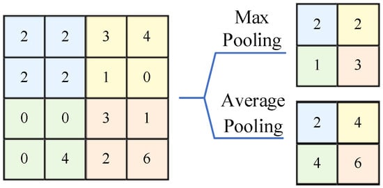
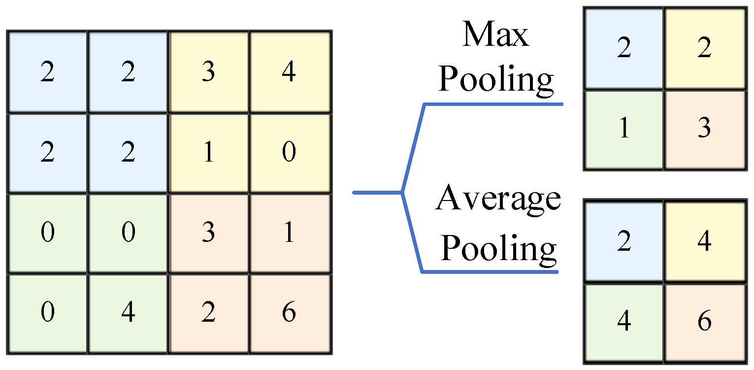
After the convolutional layer, pooling layers are usually added. The pooling operation aggregates nearby features, reduces the dimension of the input, and decreases the redundancy of feature outputs from previous layers, thereby reducing the number of training parameters and computational complexity, while providing some degree of translation in-variance. The typical pooling operations mainly include max pooling and average pooling, as shown in Figure 3. Average pooling calculates the average value within the neighborhood, while max pooling selects the maximum value within the neighbor-hood.
Figure 3.
Pool operation.
In deep neural networks, max pooling is usually adopted because it helps suppress input noise, leads to faster convergence, and improves generalization ability. For an input feature x, after max pooling, the output feature y is:
where r corresponds to the pooling window size. It simply outputs the maximum activation value within the selected region of the input.
2.4. Fully Connected Layer
Each neuron in a fully connected layer is connected to every neuron in the previous layer. The fully connected layer usually acts as the high-level structure of a deep neural network and is finally connected to a Softmax classifier to obtain the probability values of different classes. The Softmax function, also known as the normalized exponential function, outputs the probability that each input sample belongs to each category, and the sum of all category probabilities equals 1. For input xi, softmax classifier predicts the probability of belonging to yj category, and its expression is:
Among them, c corresponds to the specific number of classes, and denotes the probability output that the i-th sample belongs to class c. Similar to the learning process of a feedforward neural network, the CNN can be effectively trained by minimizing the cross-entropy loss function:
where n is the number of training samples. The parameters of the output layer can be updated using Equation (7), and the parameters of the other layers can be adjusted according to the backpropagation algorithm and the rules of stochastic gradient descent.
Moreover, graph-based representation learning has also shown strong potential in mechanical intelligence [21]. Qi et al. proposed an attention-guided graph isomorphism learning framework for simultaneous fault diagnosis and remaining useful life prediction, demonstrating the advantages of structured feature modeling in PHM tasks [22].
3. Cyclic Spectral Coherence
Among non-stationary signals, there is a type of signal whose statistical characteristics change in a single-period or multi-period manner. Such signals are called cyclostationary signal. Different from stationary signals, cyclostationary signals are not periodic signals but are generated by periodic motion mechanisms. Due to their unique periodic stationary characteristics, these signals can be characterized by the second-order statistics of cyclostationarity [23]. Building upon this foundation, Professor Antoni, considering the spectral characteristics of specific components like gears and bearings when faults occur, systematically analyzed and improved issues existing in cyclic spectral analysis algorithms, such as spectral estimation, frequency resolution, and computational speed, significantly promoting the application of cyclic spectral analysis technology in the field of mechanical fault diagnosis [24].
When faults occur in rotating machinery, their vibration signals exhibit cyclostationary characteristics. Cyclic spectral analysis technology can be employed to effectively separate interference signals from fault signals, thereby detecting and identifying their hidden periodic behaviors [25,26]. Cyclic spectral correlation theory generally uses the cyclic autocorrelation function or the cyclic spectral density to describe the cyclostationarity of a signal. For a cyclostationary signal x(t), the second-order moment of cyclostationarity is defined as the instantaneous autocorrelation function with period , which can be described as:
where denotes the complex conjugate of x(t), is the time lag, and represents the statistical average. Since the instantaneous autocorrelation function is periodic with respect to t with period , the cyclic instantaneous autocorrelation function can be obtained by:
where α is defined as the cyclic frequency. From Equation (10), it can be seen that the cyclic instantaneous autocorrelation function is the Fourier coefficient relative to the time-lagged signal x(t + τ/2)x × (t − τ/2)x(t + τ/2)x × (t − τ/2). The second-order statistics of cyclostationarity can be estimated by performing a Fourier transform on the cyclic instantaneous autocorrelation function, which is called the Cyclic Spectral Correlation (CSC):
CSC can be defined as the double Fourier transform of the signal. It is a function of the spectral frequency f and the cyclic frequency α. Unlike classical spectral analysis, it provides an additional frequency dimension, revealing the signal’s carrier and its modulation components. The spectral frequency f is related to the carrier component, while the cyclic frequency α is related to its modulation. When α equals zero, it corresponds to the classical power spectrum of a stationary signal. When α is not equal to zero, it represents the power spectrum for that specific cyclic component.
Furthermore, the Cyclic Spectral Coherence (CSCoh) is used to measure the degree of correlation between two spectral components:
CSCoh can be interpreted as a whitened version of the CSC. It tends to apply weighted averaging to amplitudes in different energy regions, thereby enhancing weak periodic components in cyclostationary signals [27].
4. Subspace Transfer Learning
The core of transfer learning lies in distribution alignment. By reducing the distribution discrepancy between the source domain and the target domain, domain knowledge can be transferred and reused. For the experiments in this study. Source Domain: Refers to bearing vibration data with complete fault labels. This dataset is used to train the model’s initial feature extraction and diagnostic capabilities. Target Domain: Refers to bearing vibration data without fault labels. The data distribution of the target domain diverges from that of the source domain due to a domain shift induced by factors such as varying operating conditions, equipment models, or environmental noise. The model must adapt to this new distribution and perform accurate diagnosis. In the distribution alignment stage, subspace transfer learning does not require label information for the source domain training data or the target domain testing data, and therefore belongs to an unsupervised transfer learning method. It usually assumes that the source domain data and the target domain data have a low-dimensional representation in the transformed feature subspace, and the alignment between the source and target domains is completed in this low-dimensional subspace. The subspace can be obtained through feature extraction, dimensionality reduction, and other feature transformation techniques. According to the form of feature transformation, subspace transfer learning methods can be divided into two types: manifold learning-based methods and statistical feature alignment-based methods.
Manifold learning algorithms are unsupervised dimensionality reduction methods. Their essence is to map high-dimensional data into a low-dimensional manifold space through certain nonlinear mappings. By solving the low-dimensional embedding, the dimensionality of high-dimensional data is reduced while retaining as much information as possible from the high-dimensional space. Common manifold learning methods include Isometric Mapping (ISOMAP), Laplacian Eigenmaps (LE), Local Linear Embedding (LLE), and Neighborhood Preserving Embedding (NPE) [28].
In manifold-based subspace transfer learning, a typical method is the Geodesic Flow Kernel (GFK) [29]. On a Grassmann manifold, it assumes that source domain data and target domain data are points on the manifold subspace. By connecting the geodesic between them and integrating the manifold functions along the geodesic, the geodesic flow can be solved. The source and target domain data are then projected onto the manifold subspace, and the geodesic flow is used to reduce the discrepancy between them, achieving subspace feature alignment. Finally, a KNN classifier is trained to complete the classification task.
Statistical feature alignment-based transfer learning methods compute the statistical features of the source and target domains in the mapped feature subspace based on unlabeled domain information through linear or nonlinear transformations, and further align the feature distributions of the two domains. The aligned data can be used for learning and classification with traditional machine learning methods.
A representative early method is Subspace Alignment (SA) [30]. Its basic idea is as follows:
First, PCA is applied to the source domain data and the target domain data for dimensionality reduction. The first d eigenvectors corresponding to the top d eigenvalues are selected to construct the d-dimensional subspace feature matrices and (,). It is easy to verify that both and are orthogonal matrices (, ). Then, by finding a linear transformation matrix M that maps the source subspace matrix into a new transformed space to minimize the difference between the source and target subspace matrices, the objective function is formulated as:
where denotes the Frobenius norm, i.e., the sum of squares of all elements. The solution of the transformation matrix M is:
Since the source-domain matrix and the target-domain matrix are both composed of d eigenvectors obtained from PCA transformation, and , the following theorem holds:
Thus, Equation (12) can be rewritten as:
The optimal solution of the transformation matrix is therefore . When , the optimal solution M becomes an identity matrix. Under the new transformation matrix, the source subspace matrix becomes , where is defined as the source-domain coordinate system aligned to the target domain. Hence, the basic process of the Subspace Alignment method can be summarized as shown in Algorithm 1.
| Algorithm 1. The SA Algorithm Description: Pseudocode of the SA Algorithm. |
| Step 1: Define source-domain data S, target-domain data T, source-domain labels Ls, and subspace dimension d Step 2: Use PCA for dimensionality reduction in the source domain to compute the source subspace matrix: Step 3: Use PCA for dimensionality reduction in the target domain to compute the target subspace matrix: Step 4: Compute the source-domain coordinate system aligned with the target domain: Step 5: Map the source-domain data S to the new subspace coordinate system: Step 6: Map the original target-domain data to the target-domain coordinate system: Step 7: Train a classifier using the aligned transformed data: Step 8: Use the trained classifier to predict the classes/labels of the target-domain data: Lt |
5. Convolutional Neural Network and Subspace Transfer Based Layer Adaptation Feature Enhancement and Fault Diagnosis Model
Based on the classical LeNet-5 architecture, a CNN fault diagnosis model is constructed, and the cyclic spectral analysis technique is adopted to transform the raw vibration signals, where the transformed cyclic spectral coherence 2D mapping is used as the input of the CNN. In the design of the CNN structure, following the same network construction strategy as LeNet-5, the proposed CNN designs the basic CNN architecture by stacking two convolutional layers, pooling layers, fully connected layers, and a Softmax classifier, which is used to learn and extract high-dimensional features from the 2D CSCoh spectral mappings. Furthermore, in order to effectively enhance the feature learning capability of the CNN and reduce the mismatch between source-domain training data and target-domain testing data, two unsupervised adaptation layers are constructed based on the subspace transfer learning technique from the perspective of statistical feature alignment, aiming to align the feature distributions of the two domains.
5.1. Unsupervised Layer Adaptation Technique Based on Statistical Feature Alignment
Compared with manifold-learning-based transfer learning methods, the statistical feature alignment approach in subspace transfer learning has the advantage that it can directly align the extracted features without requiring the computation of multiple subspace matrices, thereby significantly reducing additional hyperparameter selection and tuning processes and providing a simpler yet more effective solution. In the constructed CNN diagnosis model, the features extracted by the CNN from the original cyclic spectral input signals are used as subspace features. Meanwhile, based on the statistical characteristics of unlabeled data, two unsupervised adaptation layers—group normalization and correlation alignment—are constructed. The group normalization adaptation layer performs mean and variance normalization along the channels for each batch, ensuring that each batch of source-domain training data and target-domain testing data follows a distribution with zero mean and unit variance. The correlation alignment adaptation layer, starting from the covariance matrices of the two domains, further constructs a linear transformation matrix to minimize the difference between the two covariance matrices, thus aligning the second-order statistical features of the source-domain training data and the target-domain testing data. In this way, the adaptive capability of the features learned by the CNN is effectively improved.
- (1)
- Group Normalization Adaptation Layer
Feature normalization in deep neural networks is an unsupervised data processing method. In 2015, Google proposed the Batch Normalization (BN) method, which performs global feature normalization by computing the mean and variance of each batch along the batch dimension to reduce the distribution differences across layers. This method can effectively improve the convergence speed and learning capability of the model, becoming a standard technique in deep learning, and it has been applied in recent deep neural network fault diagnosis frameworks to enhance the network’s feature learning and classification capability [31,32].
The above method employs BN by performing mean and variance normalization along the batch channels for each batch of data, ensuring that each training batch follows a distribution with zero mean and unit variance. However, during the testing phase, the normalization relies on a weighted average of the statistical information from the training data, which cannot guarantee that each testing batch follows a distribution with zero mean and unit variance. Therefore, it cannot effectively align the statistical features of the two domains. Moreover, BN is sensitive to small batch inputs, because small batch sizes tend to produce inaccurate statistical estimates. Such inconsistent estimates may negatively affect training, causing instability in the learned features and degraded diagnostic performance on testing data.
For the adopted cyclic spectral coherence 2D graphical inputs, from the perspective of visual representation, the input channels of each image are not completely independent and exhibit mutual correlations and information redundancy [33,34]. Therefore, for the adopted cyclic spectral coherence 2D mapping inputs, to obtain more effective feature representations, the Group Normalization (GN) technique is introduced as an alternative to BN [35]. On one hand, GN eliminates the influence of BN on the statistical data of small batch samples; on the other hand, GN computes the statistical characteristics directly for each testing sample during the testing phase, ensuring that each testing batch has zero mean and unit variance. As a result, it can effectively achieve the alignment of the statistical features (zero mean and unit variance) between the source-domain training data and the target-domain testing data, thereby enhancing the learning capability of the network.
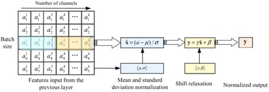
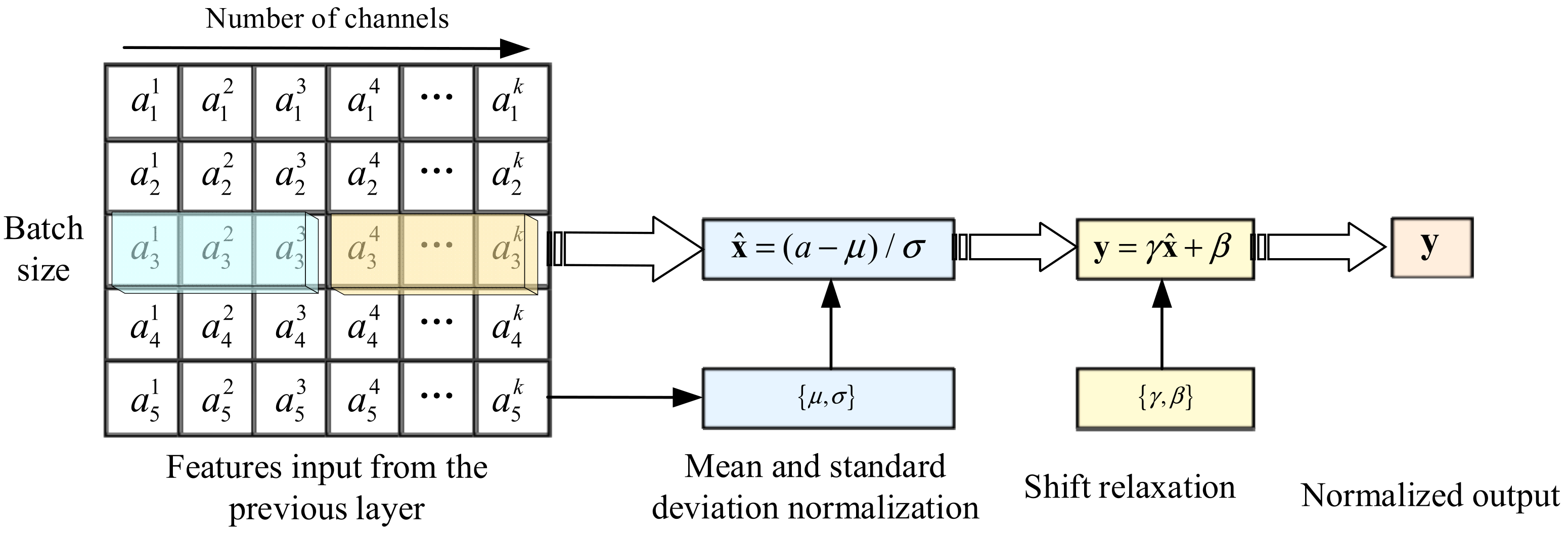
Different from the BN method, GN divides the channels into G groups and computes the mean and variance within each group, normalizing the features along the channel axis for each sample in the G groups, as shown in Figure 4. Therefore, the computation of GN is independent of batch size, enabling the network to achieve statistical feature alignment under different batch sizes and obtain stable outputs.
Figure 4.
Group normalization applied to the input features.
In GN, the input is , , where N denotes the batch size, H and W are the height and width of the input data, respectively, and C is the number of channels. The parameter M is defined as the number of channels per group, M = C/G. G is the number of groups, whose value should not exceed the number of channels. For each group, GN computes the mean and variance of each batch input along the axes:
Then, for the output of the previous layer, normalization is performed by subtracting the mean and dividing by the standard deviation:
where and represent the trainable scaling and shifting parameters, respectively, which are used to maintain the learning capability of the network. During the testing phase, since it does not depend on batch size, GN can directly compute the mean and variance of the testing data and normalize the data, ensuring that the output features of the source-domain training data and target-domain testing data are aligned: , and simultaneously . This guarantees that the network can adaptively adjust the data distribution according to the input, and even when the batch size or distribution differences change significantly, the classification performance remains stable, thereby ensuring good classification and generalization capability [35].
- (2)
- Correlation Alignment Adaptation Layer
For the input source-domain training data , , and the target-domain testing data , , where corresponds to the dimensionality of the input samples, the output features at the last fully connected layer of the constructed CNN after feeding the training and testing data can be denoted as and , respectively. Let and , and , and represent the feature means, feature variances, and feature covariance matrices of the source-domain training data and target-domain testing data after the fully connected layer of the network. In the previous CNN structure, since the GN adaptation layer has already been embedded in the fully connected layer to perform group normalization on the features of the training and testing data, the feature inputs of this layer can easily satisfy and . However, the GN adaptation layer cannot guarantee , meaning that the network cannot further align the second-order covariance statistical features of the training and testing data. This may lead to significant performance degradation of a classifier trained on the training data when applied to new testing data.
Therefore, in order to further enhance the representation capability of deep features, the transfer learning technique of Correlation Alignment (CORAL) [36] is introduced, and a correlation alignment adaptation layer (CORAL Layer) is embedded into the CNN diagnosis model. The CORAL adaptation layer minimizes the second-order statistics (covariance matrices) of the source-domain and target-domain features and utilizes the statistical information of the testing data to adjust the feature distribution of the training data, thereby effectively enhancing the representational capability of the training features and ultimately improving the classification ability of the network. After the source-domain and target-domain data are fed into the CNN and the feature representations are obtained at the fully connected layer, their covariance matrices can be defined as:
where represents the identity matrix, and denotes the mean of each feature dimension. Therefore, to minimize the second-order statistics (covariance matrices) of the two types of features, it is necessary to construct a linear transformation matrix A to map the source-domain features into a new feature space. The new source-domain features are then , and the corresponding new covariance matrix is . Thus, the final optimization function is:
where denotes the Frobenius norm of a matrix. When the rank of is greater than that of , i.e., , the solution of Acan be easily obtained such that . However, in practice, the acquired data usually lie on a low-dimensional manifold with an intrinsic dimensionality much lower than the original feature dimensionality, causing the covariance matrices to be low-rank, and thus the above condition is not easy to satisfy. Therefore, reference [36] performs whitening and coloring transformations on the features. The final algorithmic solution is shown in Algorithm 2.
| Algorithm 2. Description of the Correlation Alignment (CORAL) Algorithm: CORAL Unsupervised Feature Adaptation Layer. |
| Step 1: After passing through the CNN fully connected layer, obtain the training and testing data features and Step 2: Compute the covariance matrices and of the training and testing data features using Equations (20) and (21). Step 3: Perform correlation whitening on the obtained training data features: Step 4: Perform coloring transformation on the whitened source-domain feature data: Step 5: Output the new source-domain feature data after whitening and coloring transformations. |
5.2. CNN Fault Diagnosis with Combined GN and CORAL Adaptation Layers
For the obtained raw vibration signals, preprocessing is performed using cyclic spectral analysis to obtain the CSCoh mapping images, which extract the discriminative fault pattern features of each category and serve as the input to the CNN, thereby effectively reducing the difficulty of CNN feature learning. Then, a CNN diagnosis model using the CSCoh 2D mapping images as input is constructed. Based on the designed GN and CORAL adaptation layers, the GN adaptation layer is introduced into the network to perform group normalization on the deep features of the two domains and align the mean and variance statistical features, while the CORAL adaptation layer is further introduced to align the second-order covariance statistical features of the two domains, thereby effectively enhancing the capability of deep feature learning and generalization.
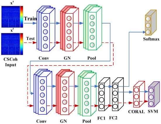
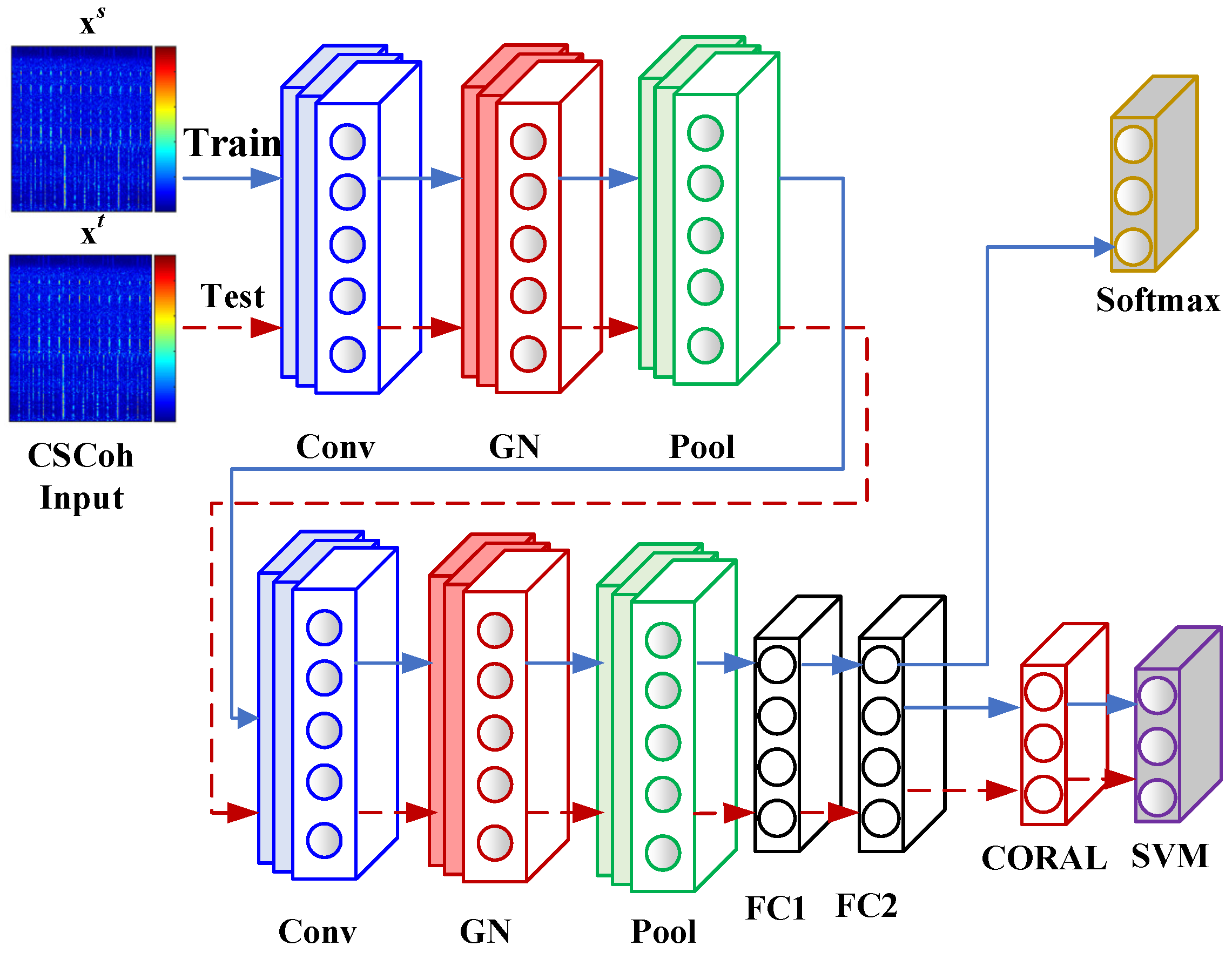
The proposed CNN fault diagnosis framework with combined GN–CORAL adaptation layers is shown in Figure 5. The constructed CNN includes convolution layers (Conv), group normalization adaptation layers (GN), pooling layers (Pool), convolution layers (Conv), group normalization adaptation layers (GN), pooling layers (Pool), two fully connected layers FC1 and FC2, a Softmax branch, and another branch with a CORAL adaptation layer and an SVM classification layer. Therefore, the learning process of the network can be divided into two stages. In the first stage, the branch consisting of Conv–GN–Pool–Conv–GN–Pool–FC1–FC2–Softmax is trained using the training data to obtain a trained CNN diagnosis model with deep feature extraction capability. In the second stage, the Softmax classifier is removed, and at this point, the CNN acts as a feature extractor. A CORAL adaptation layer is further added after the fully connected layer to perform second-order covariance statistical correlation alignment, and an SVM is introduced to train on the transformed training features and perform testing on the test data.
Figure 5.
CNN fault diagnosis framework with combined GN and CORAL adaptation layers.
Therefore, the CNN diagnosis procedure with embedded GN–CORAL adaptation layers based on two-stage training can be summarized as follows:
- (1)
- Collect bearing vibration signals under different working conditions, further segment them, and divide them into training and testing datasets. Then, apply cyclic spectral analysis to each sample to obtain the CSCoh 2D mapping images for each health condition, and scale the images to the size of 112 × 112 considering the input dimensionality and computational cost, obtaining the dimension-reduced features as the input to the CNN.
- (2)
- Design the corresponding convolution and pooling layers, and construct the CNN diagnosis model by stacking multiple convolution layers, pooling layers, and fully connected layer structures. Embed the GN adaptation layer into the CNN diagnosis model to perform group normalization along the channels on the feature outputs, aligning the mean (zero mean) and variance (unit variance) of the training and testing data. Further add the CORAL adaptation layer into the fully connected layer, and use the second-order statistical information of the testing data to align the covariance matrices of the two domains, thereby effectively enhancing the feature representation capability of the deep neural network, and input the enhanced features into the constructed SVM for learning and classification.
- (3)
- Feed the training data into the CNN branch model consisting of Conv–GN–Pool–Conv–GN–Pool–FC1–FC2–Softmax, and minimize the cross-entropy loss function between the output and the ground-truth labels. The backpropagation algorithm is used to compute gradients, and stochastic gradient descent is used to optimize the network parameters of each layer until the CNN branch diagnosis model reaches the required number of iterations or classification accuracy. Training is then stopped, and the trained model is obtained.
- (4)
- Remove the Softmax classifier, and feed the training and testing data into the CNN. At this stage, the CNN functions as a deep feature extractor. The corresponding training and testing features are output after the fully connected layer. Based on the added CORAL adaptation layer, the covariance information of the testing features is used to readjust the obtained training features so that the second-order statistical properties of the training and testing features are aligned. The adapted training features are then used to train an SVM classifier, which subsequently performs classification and diagnosis on the testing data.
6. MFPT Bearing Diagnosis Experiments Under Different Loads
6.1. Dataset
Since many rolling bearings in semiconductor manufacturing equipment are very similar to benchmark rolling bearings. In order to commercial and economic disputes, the benchmark rolling bearing dataset is used to replace the rolling bearings of semiconductor manufacturing equipment to verify the effectiveness of the proposed technique.
The rolling bearing dataset used in this experiment is taken from the publicly available dataset of the Society for Machinery Failure Prevention Technology (MFPT), shared by Dr. Eric Bechhoefer [37]. The MFPT dataset includes three health conditions: normal condition, inner race fault, and outer race fault. The data used in the experiment are described as follows: (1) Normal data (NC). This category contains three files recorded under the same load. Each file contains 6 s of sampling length, with a sampling frequency of 97,656 Hz, an input shaft rotational speed of 25 Hz, and a load of 270 pounds. (2) Inner race fault data (IF). This category contains three files recorded under different loads. Each file is sampled for 3 s at a sampling frequency of 48,828 Hz, with an input shaft rotational speed of 25 Hz. The loads are 0, 50, and 100 pounds, respectively. (3) Outer race fault data (OF). This category contains three files recorded under different loads as well. Each file is sampled for 3 s at a sampling frequency of 48,828 Hz, with loads of 25, 50, and 100 pounds, respectively. For each fault type, 0.5 s samples are extracted, and CSCoh mapping images are obtained using cyclic spectral analysis. For each health condition under each load, a total of 50 samples is obtained. The specific data types and descriptions are shown in Table 1.
Table 1.
Description of the MFPT Rolling Bearing Dataset.
Based on the obtained normal, inner race, and outer race bearing fault data, six different diagnostic tasks are constructed by dividing the data into different load intervals, as shown in Table 2. In Diagnostic Instance 1, Dataset A indicates that the normal, inner race, and outer race data are all taken from their respective first files. Dataset B indicates that the normal, inner race, and outer race data are all taken from their respective second files; Dataset C indicates that the normal, inner race, and outer race data are all taken from their respective third files. Each dataset corresponds to three fault types obtained under a specific load, and the detailed information has been previously listed in Table 1.
Table 2.
MFPT Diagnostic Datasets under Different Loads.
6.2. Cyclic Spectral Coherence Analysis (CSCoh)
In order to visually assess the structure and separability of the learned feature representations from different normalization strategies, we project the high-dimensional features from the final convolutional layer onto a 2D plane using t-Distributed Stochastic Neighbor Embedding (t-SNE). The visualizations were generated using a standard perplexity of 30 and 1000 iterations. It is important to note that these visualizations are for qualitative analysis only; all quantitative performance metrics are calculated using the original high-dimensional feature vectors.
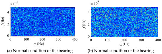
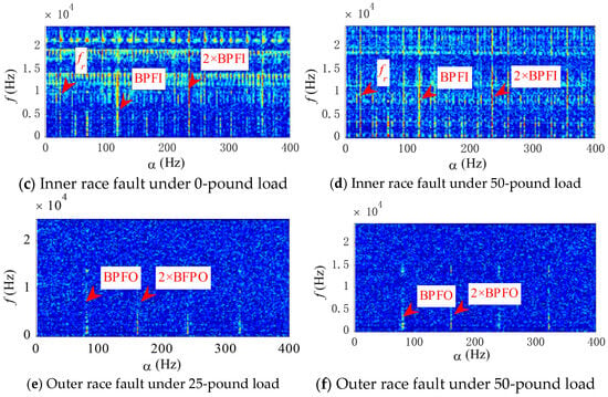
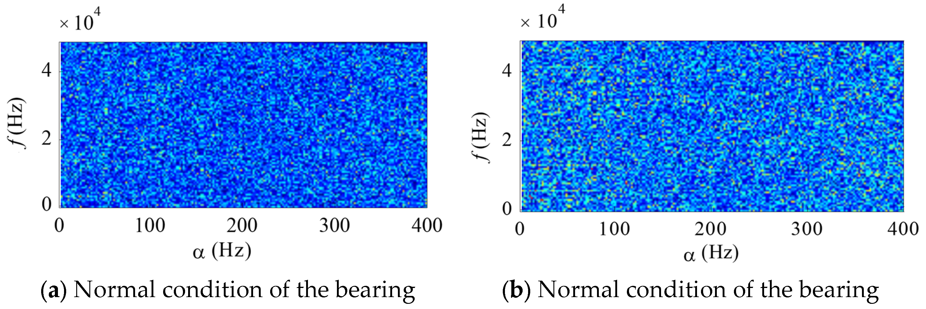
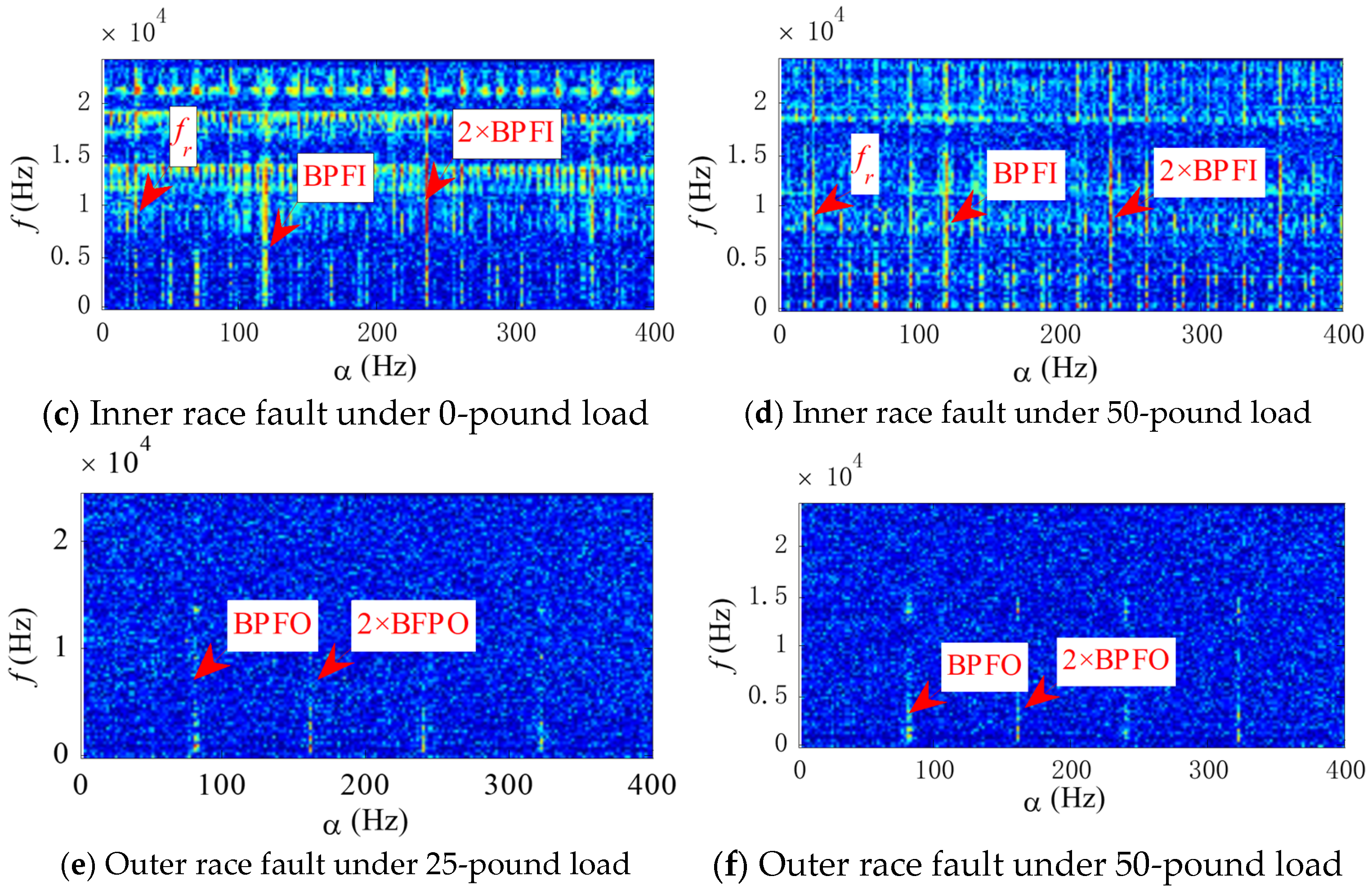
Based on the CSCoh mapping images obtained from the MFPT bearing signals, the fundamental train frequency (FTF), ball pass frequency of the inner race (BPFI), and ball pass frequency of the outer race (BPFO) are analyzed to reveal the feature extraction capability of the cyclic spectral coherence mappings. Figure 6a–f shows the CSCoh mapping images of bearing normal condition, inner race fault, and outer race fault under different loads.
Figure 6.
CSCoh analysis of different bearing health conditions.
In Figure 6a,b, it can be observed that across the entire analysis frequency range, the spectrum exhibits noise-like characteristics without any obvious frequency components representing faults, indicating that the bearing is in normal condition. For the CSCoh mappings of inner race faults under different loads, as shown in Figure 6c,d, since the rotational speed does not change under the two loads, the same frequency positions clearly exhibit the rotational frequency and its harmonics, the characteristic frequency of the inner race and its harmonics, as well as the corresponding modulation components of the inner race, clearly indicating the existence of an inner race fault. In addition, in the CSCoh mappings of outer race faults under two loads, as shown in Figure 6e,f, clear outer race characteristic frequencies and their harmonics can be observed at the same positions, without modulation components, which is consistent with the actual spectral characteristics of outer race faults.
In summary, the proposed CSCoh method presents consistent discriminative information for the same bearing health condition under different loads, and clearly reveals distinct characteristic frequency information for different health conditions. This demonstrates that CSCoh, as a feature extraction method, can provide unique feature representations for different bearing health states.
6.3. Performance Comparison of BN, GN, and GN-CORAL
For the six constructed diagnostic tasks, the CSCoh mappings are fed into the constructed CNN, and the feature learning ability of BN, GN, and GN-CORAL is further compared. In the experiments, similar to the motor bearing case, the network adopts the same CNN structure and optimization parameters for training. Each experiment is repeated ten times, and the results are shown in Table 3. For each task: The model is trained using all labeled data from the source domain. All unlabeled data from the target domain is used for domain adaptation training. To evaluate the model’s generalization performance on the target domain, 50% of the target domain data is held out as the test set. This simulates the real-world scenario of deploying the model on new, unlabeled target data.
Table 3.
Comparison of BN, GN, and GN-CORAL on MFPT Diagnostic Tasks.
From the results, it can be observed that in some diagnostic tasks, such as A→C and B→C, the average classification accuracy of BN is 98.67% (standard deviation 5.36%) and 100% (standard deviation 0), respectively, while that of GN is 97.27% (standard deviation 5.01%) and 100%. GN-CORAL achieves 99.53% (standard deviation 3.33%) and 100% (standard deviation 0). All three methods achieve very high diagnostic accuracy, indicating that the constructed CSCoh features have strong discriminative representation capability, and also demonstrating that CNN possesses powerful feature learning and classification ability. Moreover, considering all six diagnostic instances comprehensively, GN and GN-CORAL generally achieve relatively better diagnostic results with lower standard deviations. In particular, for C→B, BN achieves a classification accuracy of 98.4% with a standard deviation of 3.67%, while CNN models using GN and GN-CORAL both achieve 100% accuracy, demonstrating superior classification performance and indicating that the proposed GN and GN-CORAL schemes have better feature learning capabilities.
6.4. Comparison with Other Methods
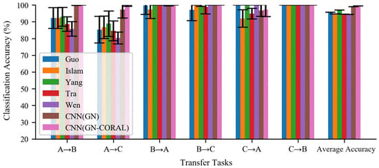
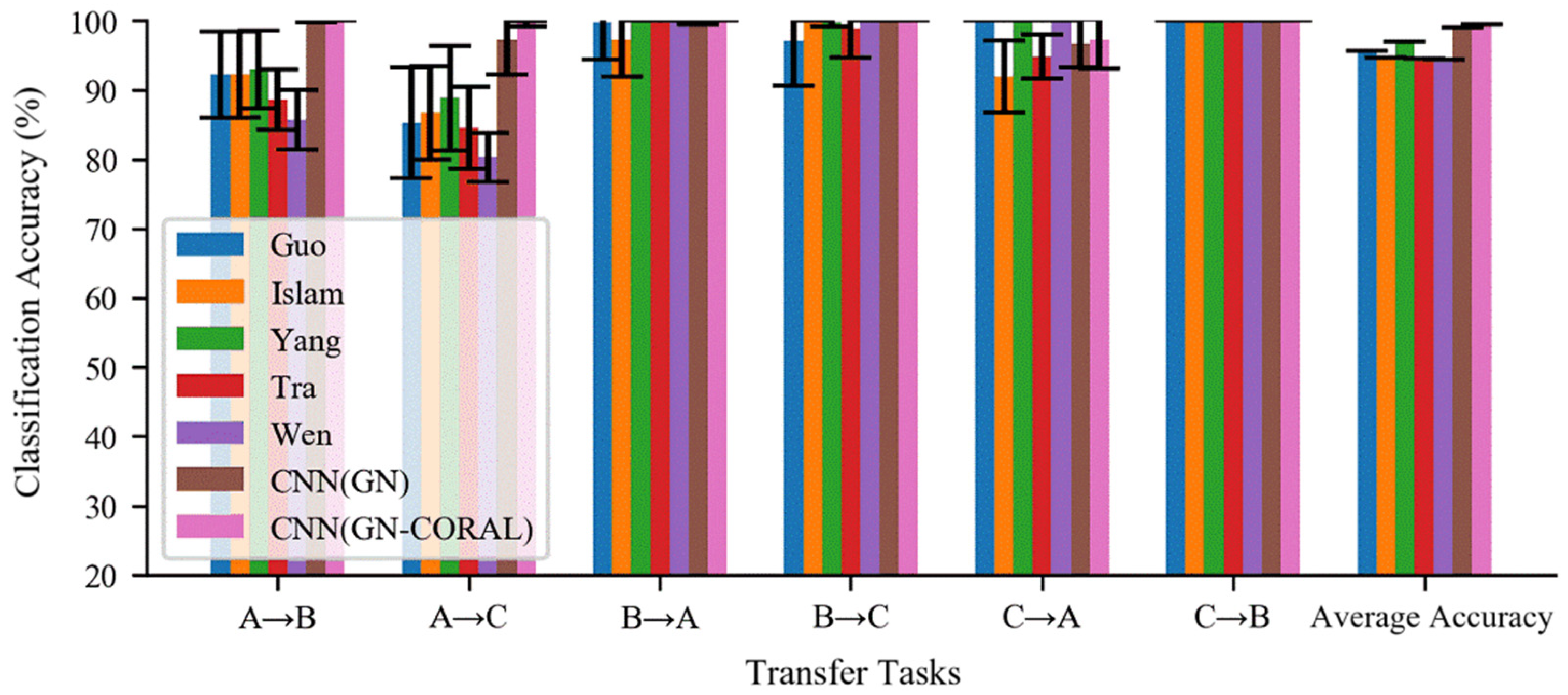
The proposed CNN (GN) and CNN (GN-CORAL) are compared with the previously introduced five CNN diagnostic networks, with network parameters kept consistent with those in the motor bearing case. The average results and standard deviations obtained on the six diagnostic tasks are shown in Figure 7.
Figure 7.
Comparison of different methods on the MFPT dataset.
In some diagnostic instances, such as B→A and B→C, all methods achieve diagnostic accuracies exceeding 90%. For C→B, 100% diagnostic accuracy is obtained, indicating that the networks can learn useful discriminative representations from the dataset, enabling high classification accuracy. However, in other tasks, such as A→B and A→C, several comparison methods exhibit significant degradation in classification performance, along with large standard deviations, indicating high sensitivity to different datasets. Considering the proposed CNN (GN) and CNN (GN-CORAL) schemes, although they do not achieve the best results on C→A, they consistently maintain high classification accuracy on the other diagnostic tasks, with the lowest accuracy being 96%, and they exhibit smaller standard deviations. This further verifies the superiority of the proposed methods.
The superior performance of the proposed CNN (GN) and CNN (GN-CORAL) methods can be attributed to their enhanced capability in handling domain shift and statistical distribution mismatch between training and testing data. While conventional CNNs rely on Batch Normalization (BN), which estimates statistics from training batches and may not generalize well under varying operational conditions, the introduced Group Normalization (GN) operates independently of batch size and aligns feature statistics per sample group. This ensures more stable and consistent normalization under different loads and small-batch scenarios.
Furthermore, the CORAL adaptation layer explicitly minimizes the discrepancy between the covariance matrices of source and target domain features, effectively aligning second-order statistics and enhancing feature invariance across domains. Combined with the discriminative CSCoh input representations that reveal cyclostationary fault characteristics, the proposed framework achieves more robust feature learning and domain adaptation, leading to higher accuracy and lower variance in cross-condition diagnosis tasks compared to baseline and existing transfer learning methods.
7. Conclusions
A semiconductor manufacturing equipment feature enhancement and fault diagnosis method based on deep learning and subspace transfer learning is proposed to improve the classification capability of mechanical equipment under different diagnostic tasks. The algorithm is validated on motor bearing data and MFPT bearing data. The results show that the CSCoh signal preprocessing adopted by the proposed method can effectively utilize the second-order statistical information of vibration signals and reveal fault components hidden within cyclostationary signals. Compared with traditional time–frequency analysis methods, it provides superior feature representation capability for bearing health conditions. In particular, by embedding GN and CORAL adaptation layers into the CNN, the method overcomes the learning instability of traditional CNN diagnostic networks under imbalanced data distributions, varying loads, and small batch-size training. It effectively enhances the deep feature learning capability of CNN and improves the diagnostic accuracy and generalization performance of the network.
In actual semiconductor manufacturing processes, the operational characteristics of key equipment such as vacuum pumps and wafer handling mechanisms are highly similar to the experimental scenarios. The proposed CNN (GN-CORAL) method improves both feature preprocessing and network learning, effectively enhancing the feature extraction and classification capabilities of CNN under different diagnostic tasks. It can be applied to online monitoring and early fault diagnosis of production-line equipment, reducing the risk of unplanned downtime and improving equipment reliability and production yield.
Author Contributions
Conceptualization, Z.W.; methodology, Z.C.; validation, Z.L.; formal analysis, P.C.; data curation, P.C.; writing—review and editing, Y.D.; supervision, Z.C.; review & editing, J.H.; funding acquisition, Z.L. All authors have read and agreed to the published version of the manuscript.
Funding
This research was funded by Characteristic innovation projects of colleges and universities in Guangdong Province (2024KTSCX296); Research platforms and projects in Guangdong Universities (2022KQNCX223); Guangdong Provincial Natural Science Foundation Project (2020JJ4316); National Natural Science Foundation of China (52205101); Start up project of scientific research on newly introduced talents of Guangzhou railway Polytechnic (GTXYR2440) and Science and technology innovation team of Guangzhou railway Polytechnic (GTXYT2402).
Data Availability Statement
The original contributions presented in this study are included in the article. Further inquiries can be directed to the corresponding author.
Conflicts of Interest
The authors declare no conflicts of interest.
Nomenclature
The following abbreviations are used in this manuscript:
| CNN | Convolutional neural network |
| PHM | Prognostics and health management |
| TCA | Transfer component analysis |
| ETCNN | Enhanced transfer convolutional neural network |
| ReLU | Rectified Linear Unit |
| ISOMAP | Isometric mapping |
| LE | Laplacian Eigenmaps |
| LLE | Local Linear Embedding |
| NPE | Neighborhood Preserving Embedding |
| GFK | Geodesic Flow Kernel |
| SA | Subspace Alignment |
| BN | Batch Normalization |
| GN | Group Normalization |
| CORAL | Correlation Alignment |
| t-SNE | t-Distributed Stochastic Neighbor Embedding |
References
- Chen, Z.; Lin, H.; Gao, Y.; He, J.; Li, Z.; Li, W.; Liu, Q. Multiscale Scattering Forests: A Domain-Generalizing Approach for Fault Diagnosis under Data Constraints. Knowl.-Based Syst. 2026, 337, 115389. [Google Scholar] [CrossRef] [Scilit]
- Qi, J.; Karimi, H.R.; Uhlmann, Y.; Chen, Z.; Li, W.; Schullerus, G. Uncertainty-Aware Sensorless Anomaly Detection Using a Reliable Indicator From Position-Guided Multi-Step Deep Decomposition Network. Reliab. Eng. Syst. Saf. 2026, 271, 112258. [Google Scholar] [CrossRef] [Scilit]
- Li, X.; Xiao, S.; Li, Q.; Zhu, L.; Wang, T.; Chu, F. The Bearing Multi-sensor Fault Diagnosis Method Based on a Multi-branch Parallel Perception Network and Feature Fusion Strategy. Reliab. Eng. Syst. Saf. 2025, 261, 111122. [Google Scholar] [CrossRef] [Scilit]
- Ma, S.; Leng, J.; Zheng, P.; Chen, Z.; Li, B.; Li, W.; Liu, Q.; Chen, X. A digital twin-assisted deep transfer learning method towards intelligent thermal error modeling of electric spindles. J. Intell. Manuf. 2025, 36, 1659–1688. [Google Scholar] [CrossRef] [Scilit]
- Netease. Deaths and 16 Injuries Caused by Elevator Falling, Yunnan Released the Accident Investigation Report [EB/OL]. Available online: https://www.163.com/dy/article/J2D6H5TC0512D3VJ.html (accessed on 17 May 2024).
- Pan, S.J.; Yang, Q. A Survey on Transfer Learning. IEEE Trans. Knowl. Data Eng. 2009, 22, 1345–1359. [Google Scholar] [CrossRef] [Scilit]
- Xie, J.; Zhang, L.; Duan, L.; Wang, J. On Cross-Domain Feature Fusion in Gearbox Fault Diagnosis under Various Operating Conditions Based on Transfer Component Analysis. In Proceedings of the International Conference on Prognostics and Health Management, Ottawa, ON, Canada, 20–22 June 2016. [Google Scholar]
- Shen, F.; Chen, C.; Yan, R. Application of SVD and Transfer Learning Strategy on Motor Fault Diagnosis. J. Vib. Eng. 2017, 30, 118–126. [Google Scholar]
- Zhang, R.; Tao, H.; Wu, L.; Guan, Y. Transfer Learning with Neural Networks for Bearing Fault Diagnosis in Changing Working Conditions. IEEE Access 2017, 5, 14347–14357. [Google Scholar] [CrossRef] [Scilit]
- Yan, R.; Shen, F.; Sun, C.; Chen, X. Knowledge Transfer for Rotary Machine Fault Diagnosis. IEEE Sens. J. 2019, 20, 8374–8393. [Google Scholar] [CrossRef] [Scilit]
- Jia, F.; Li, S.; Shen, J.; Ma, J.; Li, N. Fault Diagnosis of Rolling Bearings Using Deep Transfer Learning and Adaptive Weighting. J. Xi’an Jiaotong Univ. 2022, 56, 1–10. [Google Scholar]
- Yang, S.; Kong, X.; Wang, Q.; Cheng, H.; Li, Z. Mechanical Fault Diagnosis Based on Multi-Source Domain Deep Transfer Learning. J. Vib. Shock 2022, 41, 32–40. [Google Scholar]
- Shao, S.; McAleer, S.; Yan, R.; Baldi, P. Highly Accurate Machine Fault Diagnosis Using Deep Transfer Learning. IEEE Trans. Ind. Inform. 2018, 15, 2446–2455. [Google Scholar] [CrossRef] [Scilit]
- Han, T.; Liu, C.; Yang, W.; Jiang, D. A Novel Adversarial Learning Framework in Deep Convolutional Neural Network for Intelligent Diagnosis of Mechanical Faults. Knowl.-Based Syst. 2019, 165, 474–487. [Google Scholar] [CrossRef] [Scilit]
- Lin, H.; Huang, X.; Chen, Z.; He, G.; Xi, C.; Li, W. Matching pursuit network: An interpretable sparse time–frequency representation method toward mechanical fault diagnosis. IEEE Trans. Neural Netw. Learn. Syst. 2024, 36, 12377–12388. [Google Scholar] [CrossRef] [Scilit] [PubMed]
- Li, X.; Wu, X.; Yu, J.; Wang, T.; Shi, C.; Choi, J.-H.; Chu, F. A fault diagnosis data augmentation method integrating multimodal non-Gaussian denoising diffusion generative adversarial network. Adv. Eng. Inform. 2025, 68, 103776. [Google Scholar] [CrossRef] [Scilit]
- Xia, J.; Huang, R.; Li, J.; Chen, Z.; Li, W. Digital twin-assisted fault diagnosis of rotating machinery without measured fault data. IEEE Trans. Instrum. Meas. 2024, 73, 3531210. [Google Scholar] [CrossRef] [Scilit]
- Chen, Z.; Zhong, Q.; Huang, R.; Liao, Y.; Li, J.; Li, W. Intelligent Fault Diagnosis for Machinery Based on Enhanced Transfer Convolutional Neural Network. J. Mech. Eng. 2021, 57, 96–105. [Google Scholar]
- LeCun, Y.; Bottou, L.; Bengio, Y.; Haffner, P. Gradient-Based Learning Applied to Document Recognition. Proc. IEEE 1998, 86, 2278–2324. [Google Scholar] [CrossRef] [Scilit]
- Qi, J.; Chen, Z.; Kong, Y.; Qin, W.; Qin, Y. Attention-guided graph isomorphism learning: A multi-task framework for fault diagnosis and remaining useful life prediction. Reliab. Eng. Syst. Saf. 2025, 263, 111209. [Google Scholar] [CrossRef] [Scilit]
- Qi, J.; Chen, Z.; Uhlmann, Y.; Schullerus, G. Sensorless robust anomaly detection of roller chain systems based on motor driver data and deep weighted KNN. IEEE Trans. Instrum. Meas. 2024, 74, 3502613. [Google Scholar] [CrossRef] [Scilit]
- Antoni, J.; Xin, G.; Hamzaoui, N. Fast computation of the spectral correlation. Mech. Syst. Signal Process. 2017, 92, 248–277. [Google Scholar] [CrossRef] [Scilit]
- Borghesani, P.; Antoni, J. A faster algorithm for the calculation of the fast spectral correlation. Mech. Syst. Signal Process. 2018, 111, 113–118. [Google Scholar] [CrossRef] [Scilit]
- Mauricio, A.; Qi, J.; Smith, W.A.; Sarazin, M.; Randall, R.B.; Janssens, K.; Gryllias, K. Bearing diagnostics under strong electromagnetic interference based on Integrated Spectral Coherence. Mech. Syst. Signal Process. 2020, 140, 106673. [Google Scholar] [CrossRef] [Scilit]
- Gryllias, K.; Mauricio, A.; Qi, J. Advanced cyclostationary-based analysis for condition monitoring of complex systems. In Proceedings of the 2018 26th European Signal Processing Conference (EUSIPCO), Rome, Italy, 3–7 September 2018; pp. 385–389. [Google Scholar]
- Mauricio, A.; Qi, J.; Smith, W.; Randall, R.; Gryllias, K. Vibration Based Condition Monitoring of Planetary Gearboxes Operating Under Speed Varying Operating Conditions Based on Cyclo-non-stationary Analysis. In Proceedings of the International Conference on Rotor Dynamics, Rio de Janeiro, Brazil, 23–27 September 2018; pp. 265–279. [Google Scholar]
- Nair, V.; Hinton, G.E. Rectified Linear Units Improve Restricted Boltzmann Machines. In Proceedings of the 27th International Conference on Machine Learning (ICML-10), Haifa, Israel, 21–24 June 2010; pp. 807–814. [Google Scholar]
- Zhang, S. Research on Mechanical State Recognition Method Based on Manifold Learning. Master’s Thesis, South China University of Technology, Guangzhou, China, 2014. [Google Scholar]
- Gong, B.; Shi, Y.; Sha, F.; Grauman, K. Geodesic Flow Kernel for Unsupervised Domain Adaptation. In Proceedings of the 2012 IEEE Conference on Computer Vision and Pattern Recognition, Providence, RL, USA, 16–21 June 2012; IEEE: New York, NY, USA, 2015. [Google Scholar]
- Fernando, B.; Habrard, A.; Sebban, M.; Tuytelaars, T. Unsupervised Visual Domain Adaptation Using Subspace Alignment. In Proceedings of the IEEE International Conference on Computer Vision, Columbus, OH, USA, 23–28 June 2014; IEEE: New York, NY, USA, 2014. [Google Scholar]
- Xia, J.; Huang, R.; Chen, Z.; He, G.; Li, W. A novel digital twin-driven approach based on physical-virtual data fusion for gearbox fault diagnosis. Reliab. Eng. Syst. Saf. 2023, 240, 109542. [Google Scholar] [CrossRef] [Scilit]
- Zhang, W.; Li, C.; Peng, G.; Chen, Y.; Zhang, Z. A Deep Convolutional Neural Network with New Training Methods for Bearing Fault Diagnosis under Noisy Environment and Different Working Load. Mech. Syst. Signal Process. 2018, 100, 439–453. [Google Scholar] [CrossRef] [Scilit]
- Lowe, D.G. Distinctive Image Features from Scale-Invariant Keypoints. Int. J. Comput. Vis. 2004, 60, 91–110. [Google Scholar] [CrossRef] [Scilit]
- Dalal, N.; Triggs, B. Histograms of Oriented Gradients for Human Detection. In Proceedings of the 2005 IEEE Computer Society Conference on Computer Vision and Pattern Recognition (CVPR’05), San Diego, CA, USA, 20–25 June 2005; Volume 1, pp. 886–893. [Google Scholar]
- Wu, Y.; He, K. Group Normalization. In Proceedings of the European Conference on Computer Vision (ECCV), Munich, Germany, 8–14 September 2018; pp. 3–19. [Google Scholar]
- Sun, B.; Feng, J.; Saenko, K. Return of Frustratingly Easy Domain Adaptation. In Proceedings of the Thirtieth AAAI Conference on Artificial Intelligence, Phoenix, AZ, USA, 12–17 February 2016. [Google Scholar]
- Lee, D.; Siu, V.; Cruz, R.; Yetman, C. Convolutional neural net and bearing fault analysis. In Proceedings of the International Conference on Data Mining (DMIN), Las Vegas, NV, USA, 25–28 July 2016; The Steering Committee of The World Congress in Computer Science, Computer Engineering and Applied Computing (WorldComp): Las Vegas, NV, USA, 2016; p. 194. [Google Scholar]

Disclaimer/Publisher’s Note: The statements, opinions and data contained in all publications are solely those of the individual author(s) and contributor(s) and not of MDPI and/or the editor(s). MDPI and/or the editor(s) disclaim responsibility for any injury to people or property resulting from any ideas, methods, instructions or products referred to in the content. |
© 2026 by the authors. Licensee MDPI, Basel, Switzerland. This article is an open access article distributed under the terms and conditions of the Creative Commons Attribution (CC BY) license.