


Abstract
This study investigates the integration of reinforcement learning (RL) with Model Reference Adaptive Control (MRAC) to improve pitch-axis tracking of an aerial platform operating under nonlinear dynamics and external disturbances. A hybrid RL-MRAC framework is developed by augmenting a conventional linear MRAC controller with a bounded, online reinforcement-learning component based on SARSA-inspired temporal-difference learning. The proposed approach learns corrective control actions without requiring prior offline training or explicit knowledge of the plant’s nonlinear dynamics. A Lyapunov-based stability analysis is presented to characterize the tracking behavior under bounded uncertainties and specified adaptive-parameter assumptions. The proposed controller is evaluated through MATLAB simulations and compared with conventional Linear-MRAC, Nonlinear-MRAC, and radial basis function neural-network MRAC. The evaluation considers multiple reference trajectories, external disturbances, nonlinear parameter variations, measurement noise, and actuator constraints. Simulation results demonstrate that RL-MRAC can improve tracking performance under selected operating conditions. In the representative sinusoidal-disturbance case, the proposed controller achieves reductions of 3.64% in integral absolute error and 6.05% in integral time-weighted absolute error compared with Linear-MRAC. However, repeated simulations reveal that the improvements are dependent on the operating conditions and are accompanied by increased control-input variation. These findings demonstrate the potential of bounded residual reinforcement learning as an adaptive compensation strategy while highlighting the importance of learning design, robustness, and actuator limitations in practical applications.
1. Introduction and Related Work
Attitude control of aerial platforms such as quadrotors is inherently challenging due to unmodeled nonlinear dynamics, parameter uncertainties, and external disturbances that are difficult to capture in simplified mathematical models. Even when nominal state–space representations describe the dominant rigid-body behavior, residual effects such as aerodynamic drag, actuator nonlinearities, and ground interactions remain unaccounted for, often degrading controller performance. These limitations have motivated the development of adaptive and intelligent control strategies that can compensate for unknown dynamics in real time. This work focuses specifically on the pitch-axis attitude channel of a half-drone rotary platform, a canonical single-axis testbed for such strategies.
To highlight those challenges, surveys have documented the advancements and difficulties in quadrotor control. For instance, Emran and Najjaran [1] analyzed quadrotor dynamics and highlighted the platform’s underactuated nature, showing how adaptive and intelligent controllers have been developed to address nonlinearities while advancing modeling, stabilization, and trajectory tracking. Their review sets the foundation for approaches that bridge gaps in handling unmodeled dynamics and external disturbances.
Recent years have seen increasing interest in combining Model Reference Adaptive Control (MRAC) with Artificial Intelligence (AI) techniques such as neural networks, Gaussian processes, reinforcement learning, and fuzzy systems. These approaches have been applied in quadrotors, spacecraft, and other aerospace systems to address uncertainties, disturbances, and nonlinearities that cannot be managed by classical controllers. The following works illustrate the breadth of these contributions.
Glushchenko and Lastochkin [2] evaluated neural uncertainty compensation for quadrotor tracking. Madebo et al. [3] studied feedforward and recurrent neural networks within MRAC for quadrotor tracking in simulation. Zhou et al. [4] used a Lipschitz-constrained network for model reference adaptation and demonstrated the approach in flying inverted-pendulum experiments. Liu et al. [5] incorporated multilateral neural learning into MRAC, presented a Lyapunov stability analysis, and evaluated the controller on an inverted-pendulum system. Emran and Najjaran [6] proposed a global quadrotor tracking strategy based on adaptive dynamic surface control.
Chowdhary et al. [7] used Gaussian processes (GPs) for adaptive control. Cen et al. [8] combined modified GP regression with quaternion-based command-filtered backstepping and evaluated quadrotor tracking under perturbations in simulation. Related sparse online GP estimators were used for incremental backstepping flight control [9] and for nonlinear dynamic inversion under multirotor ground effect [10].
Recent studies have also integrated deep learning explicitly into MRAC. For example, Predictor-based Deep MRAC employed a state predictor and deep neural networks to improve quadrotor trajectory tracking, updating only the output layer online and demonstrating robust performance under time-varying disturbances [11].
Reinforcement learning (RL) has been explored as well. A regression-based RL controller was applied in a rocket landing problem, improving robustness over PID and LQG controllers, especially under wind disturbances [12]. More recently, an online actor-critic RL framework was developed for nonlinear systems with actuator failures, where stability was mathematically ensured and robust tracking achieved without explicit fault detection [13].
Residual reinforcement learning provides a more closely related architecture. Johannink et al. [14] introduced residual RL by superimposing a learned corrective policy on a conventional feedback controller. Staessens et al. [15] subsequently investigated constrained residual RL for mechatronic control, where limiting the learned residual action preserves properties of the baseline controller. Related combinations of adaptive control and RL have also been proposed. Guha and Annaswamy [16] introduced an MRAC-RL framework in which an inner-loop MRAC compensates modeling errors seen by a simulation-trained outer-loop RL policy. Abouheaf et al. [17] developed a data-driven model-reference adaptive approach based on integral reinforcement learning without requiring explicit process or reference-model dynamics in the control strategy.
Other adaptive AI-based controllers have combined multiple techniques. For instance, Wei et al. [18] combined a high-level model path-following contouring controller with an adaptive neural feedback linearization controller to manage gusts and turbulence, while Choi et al. [19] integrated neural and fuzzy controllers within a sliding mode framework, evaluating tracking robustness in simulation.
Bayraktar and Bakirci [20] examine learning-based autonomous airspace coordination under uncertainty, which provides context at the decision-making level. At the sensing level, Zou et al. [21] use onboard inertial measurements to detect multirotor propeller faults. The present study addresses low-level pitch tracking and does not model flexible-body vibration or test vibration suppression.
This study evaluates an online, bounded SARSA-inspired residual within Linear-MRAC. The learner uses a fixed 16-feature action-value approximation, without offline policy training or access to the plant nonlinear regressor. The evaluation combines a learning-based baseline, repeated-seed comparisons and sensitivity tests with a conditional analysis of the applied residual bound.
The main contributions of this work are as follows:
- Online residual learning within an MRAC backbone:A bounded residual learning architecture combines Linear-MRAC with an online, SARSA-inspired TD learner. Its implemented gate, target buffering, and weight-update schedule are specified explicitly. The learner uses no offline training and is not given the plant’s true nonlinear regressor basis .
- Practical tracking characterization:A conditional Lyapunov tracking characterization is derived under the matching condition, bounded effective uncertainty, and explicitly assumed bounded adaptive parameter errors. The scalar residual enters the two-state plant through its input matrix. A common sublevel-set argument gives conservative ultimate tracking bounds without requiring convergence of the SARSA weights. Regressor mismatch is included only when the plant and compensator actually use different regressor signals.
- Structural-knowledge versus residual-learning comparison:The primary study compares RL-MRAC with Linear-MRAC and nonlinear MRAC supplied with the true basis but not its coefficients, retaining complete single-run tracking and learning histories. An additional RBF-NN MRAC baseline, 20-seed comparisons, and sensitivity, noise, disturbance, actuator, and delay studies assess the scope of those observations.
2. Methodology
Capturing the full dynamics of a physical system in real-world applications is not trivial. Uncertainties in parameters, unmodeled dynamics, nonlinear effects, and external disturbances persist even after deriving a state-space model. Since it captures the major rigid-body behavior while intentionally leaving residual effects for the controller to handle, a nominal second-order model of the pitch channel is used as the baseline representation for this investigation. The next step is to create and evaluate adaptive controllers that can make up for these discrepancies. First, a linear MRAC structure is employed to address parametric uncertainty in the traditional manner, after which a standard MRAC that utilizes nonlinear basis functions is constructed to model unmodeled effects.
Lastly, RL-MRAC augments the adaptive baseline with a bounded residual learned online. Its empirical contribution is assessed through repeated-seed comparisons rather than assumed from the architecture.
To ensure that the comparisons emphasize the inherent differences between controllers rather than depending on aggressive tuning, modest adaptation gains are used in all cases, reflecting practical considerations such as noise sensitivity.
2.1. System Model
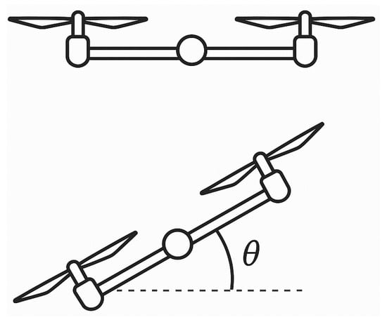
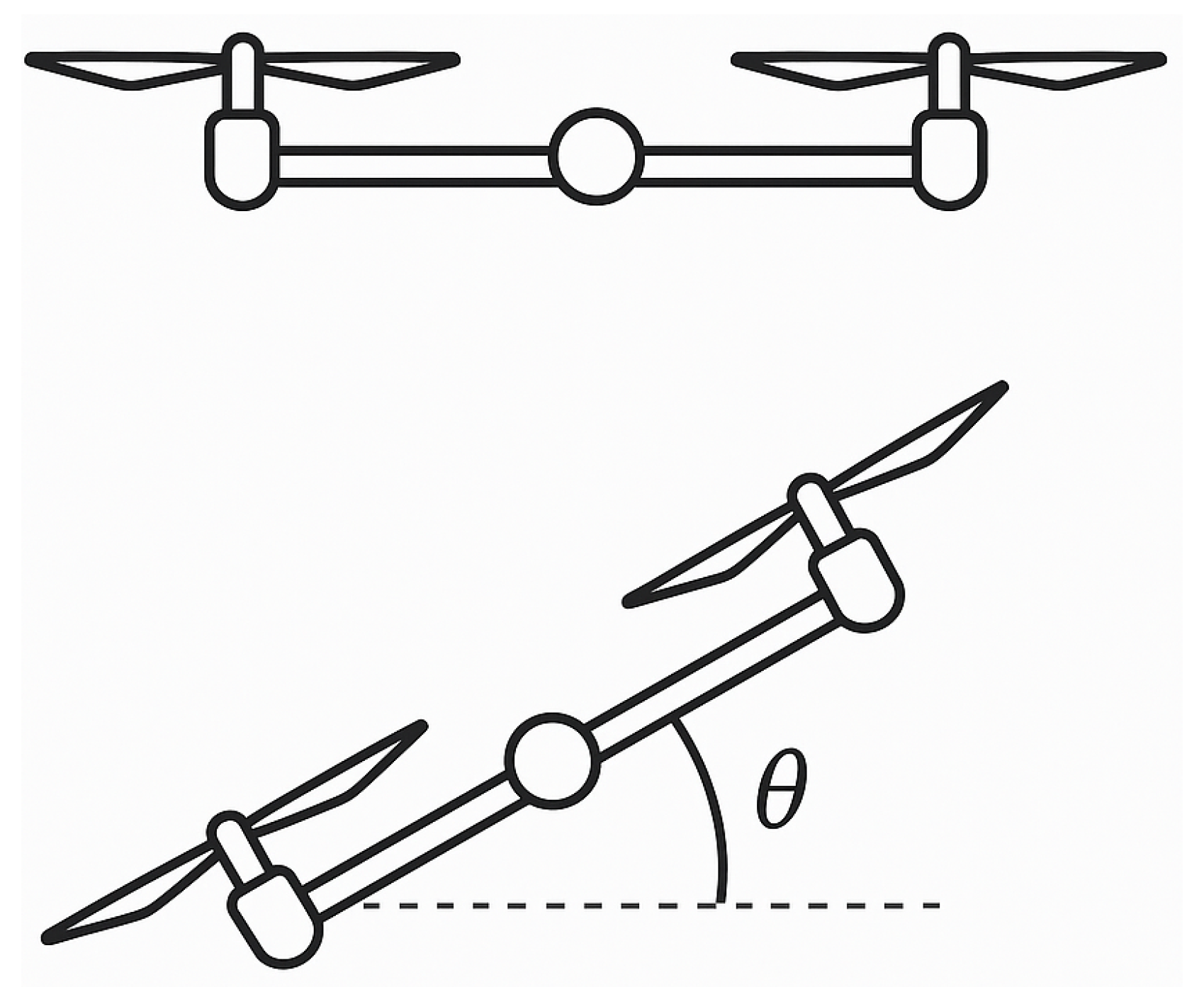
The plant considered in this work is a single-axis rotary setup representing the pitch channel of a half-drone aerial platform (Figure 1). Starting from Newton’s second law for rotational motion, the dynamics can be written as
where J is the rotational inertia, D is the viscous damping coefficient, is the stiffness constant, is the actuator’s torque gain, is the pitch angle, is the input voltage applied to the actuator, and represents external disturbances.
Figure 1.
Half-drone schematic showing the pitch axis and pitch angle relative to the horizontal.
Defining the state vector as
with the pitch angle and the pitch rate, the system can be represented in continuous-time state–space form:
Although the controller is not given the precise parameter values, this model represents the nominal pitch dynamics. Other nonlinear parameters that affect the dynamics are not explicitly known, and inertia, damping, and stiffness are examples of unknown quantities in practice. It is assumed that the controller is simply aware of the state-space equation structure. The numerical constants used in the simulations are provided in the results section. This configuration mimics real-world circumstances in which precise plant models are not available and adaptability is necessary to fill the gap.
2.2. Control-Oriented Nonlinear Plant Model
For controller design and stability analysis, the nominal pitch dynamics are augmented with a matched nonlinear uncertainty term. The resulting control-oriented representation is
where the state vector remains
with the pitch angle and the pitch rate, and u denotes the control input applied to the actuator. The input effectiveness is assumed to be an unknown positive constant; only its sign is assumed known. Accordingly, the adaptive laws use the known input direction , while is accounted for in the Lyapunov analysis. The additional matched nonlinear dynamics are represented by , where is an unknown coefficient vector and is the nonlinear regressor of dimension n. The regressor vector contains terms that model nonlinear effects. The specific coefficients and regressor entries used in simulation are provided in the results section.
Here denotes the regressor actually supplied to the simulated plant, whereas will denote the nonlinear-MRAC compensator regressor. For an instantaneous plant, . If a sampled input is used in the plant, that delayed signal is part of and must also be retained in the analysis. The scalar is expressed in input-equivalent units; multiplication by maps it into the state derivatives. The vector is a separate additive state disturbance.
2.3. Role of the Regressor: Information Available to Each Controller
A natural question is how the predefined regressor differs conceptually from simply incorporating the nonlinear terms into the system model before controller design. The distinction lies in what each controller is permitted to know, which is the central variable of this study:
- In the plant simulation, the pair constitutes the ground-truth unmodeled dynamics. It plays the role that physical effects (drag, friction, saturation) would play on hardware: it exists in the plant whether or not any controller knows about it.
- Nonlinear MRAC is given the basis and does not receive the coefficient vector . Incorporating the nonlinearities directly into the design model would require knowing , which would reduce the problem to exact feedback cancellation and eliminate the need for adaptation altogether. Because is unknown, the controller must still estimate online through the adaptive law; the known basis represents the best case of structural knowledge, not model knowledge.
- Linear-MRAC and RL-MRAC are given neither nor . RL-MRAC must discover a corrective action purely from the reward signal.
This graded information structure—access to the true nonlinear regressor basis for nonlinear MRAC versus no access to that basis for Linear-MRAC and RL-MRAC—allows the study to examine the value of explicit plant-structure information under the tested operating conditions.
2.4. Reference System
A second-order reference model is used to define the desired closed-loop behavior. This model serves as the trajectory that the adaptive controllers are supposed to follow and reflects the desired transient response in terms of rise time, damping, and steady-state gain. The reference system’s dynamics are provided by
where
denotes the reference states (reference pitch angle and reference pitch rate), and r is the external command input. The matrices and are chosen to yield a stable second-order system with a moderately fast response and limited overshoot.
For the stability analysis that follows, it is required that be Hurwitz. In this case, for any symmetric positive-definite matrix , there exists a unique symmetric positive-definite solution to the algebraic Lyapunov equation:
This guarantees the existence of a quadratic Lyapunov function candidate that can be used to analyze the boundedness and convergence of the tracking error dynamics in later sections. The specific numerical choices of , , Q, and P used in the simulations are provided in the results section.
2.5. Linear MRAC
The first adaptive controller considered is the Linear Model Reference Adaptive Controller (Linear-MRAC), a classical formulation widely presented in standard adaptive control literature [22], which handles parametric uncertainty. The design objective is to force the plant states x to track the reference model states .
The control input is defined as a linear adaptive law of the form
where
- are adaptive feedback gains applied to the states, and
- is the adaptive gain applied to the reference input .
The ideal (unknown) parameters would cancel the parametric mismatch between the plant and the reference model. Since these values are not available, the estimates are adjusted online using adaptive update laws.
For clarity, two error quantities are distinguished throughout this work. The model-reference tracking error used in the adaptive laws and Lyapunov analysis is defined as
Separately, the pitch command-tracking error used in the reinforcement-learning reward and in the command-tracking metrics reported for the ensemble is defined as
The adaptive laws update and based on e, ensuring that the closed-loop system drives the error towards zero.
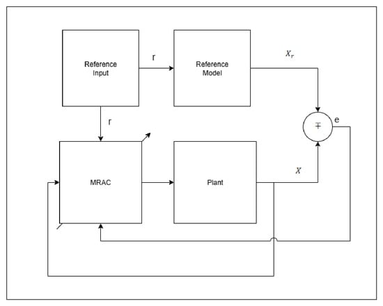
Conceptually, the Linear-MRAC structure consists of the following:
- A reference model block that generates the desired trajectory from the input r,
- An adaptive controller block that computes u from the plant states and the command input using the adaptive gains,
- An update mechanism that adjusts the gains and online in response to the tracking error.
To implement this control law adaptively, the gains are updated online using the following differential equations:
where and are adaptation gains, P is the Lyapunov solution associated with the reference model, and is the input matrix of the plant. These update laws continuously adjust and such that the tracking error is driven toward zero.
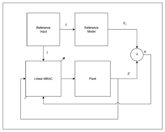
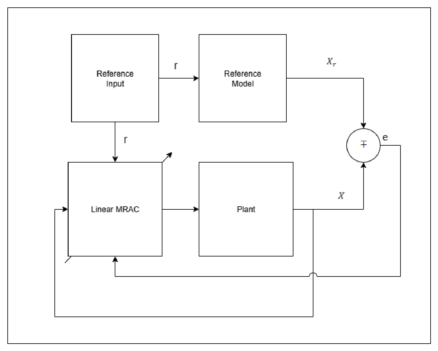
The adaptation process can be visualized in block form, as shown in Figure 2. The diagram illustrates how the tracking error feeds into the update laws, the integrators accumulate the parameter estimates, and the updated gains are applied to the plant states and reference input to generate the control signal.
Figure 2.
Linear MRAC block diagram.
This controller serves as the baseline adaptive approach for comparison with the nonlinear MRAC and the RL-augmented MRAC presented later.
2.6. Nonlinear MRAC Controller
Building on the Linear-MRAC formulation [22], the Nonlinear MRAC extends the control law by incorporating a basis function vector that captures unmodeled nonlinear dynamics. As discussed in Section 2.3, this controller is given the basis but not the coefficients . The control input is defined as
where
- are adaptive gains applied to the states,
- is the adaptive gain applied to the reference input ,
- is a vector of nonlinear basis functions evaluated using the current state and the previous controller-sample input , where , and
- is the adaptive parameter vector estimating the unknown nonlinear coefficients.
As in the linear case, the tracking error (7) measures the deviation between the plant and the reference model. The gains and are updated by (9) and (10), respectively. The nonlinear parameter update is
where is the nonlinear adaptation gain, and P is the Lyapunov solution from the reference model. These update laws allow the controller not only to compensate for parametric mismatch but also to cancel nonlinear residual dynamics.
The nonlinear MRAC structure (Figure 3) adds an adaptation loop driven by . The one-sample evaluation is a numerical implementation choice to avoid an implicit input equation, rather than an intrinsic requirement of nonlinear MRAC. A current-input implementation would require solving that implicit equation or otherwise establishing a causal realization. A delay shared by the plant and compensator does not, by itself, create a regressor mismatch. Consequently, the observed disturbance-rejection ranking cannot be attributed to a controller-only delay without a separate controlled comparison. The present results compare the implemented architectures rather than every possible realization of nonlinear MRAC.
Figure 3.
Nonlinear MRAC block diagram.
2.7. RL-MRAC
The evaluated implementation augments Linear-MRAC with bounded, SARSA-inspired temporal-difference learning with linear function approximation [23]. Its buffered target and solver-output update schedule differ from conventional forward-transition SARSA and are retained explicitly in the numerical comparisons. The adaptive baseline is the Linear-MRAC input (6). At sample k, a raw action is selected by an -greedy policy using
The nominal action set and its bound are
The applied residual includes the implemented signed gate:
and the total input is
The raw action is held between samples, while the gate is evaluated with the evolving reference-model and plant states. Under measurement noise, the measured plant state replaces x in the controller, gate, and learner. This asymmetric gate is an implementation choice, not a stability requirement; a separate ablation compares it with no gate and with an absolute-error gate.
For the square-wave studies, the reward uses command error and penalizes the raw selected action even when the gate suppresses it:
Here , , and weight squared command error, squared selected action, and squared pitch rate, respectively. An angle error of rad and a rate of rad/s each contribute to the penalty; an action of magnitude 4 contributes . These empirical weights express a numerical trade-off between differently scaled quantities, not an optimal or dimensionless physical cost. No reward-weight sensitivity study is claimed.
The actual buffered target at a major sample is
This target results from the original scalar delay acting across a two-element state frame. Its first entry is a previous rate and its second is a current angle; it is not a physical next-state vector in the defined angle–rate ordering. A second -greedy selector supplies at this target, using the current reference. Each learner evaluation computes
The main experiments preserve one major-time evaluation and three additional, lagged solver-output evaluations per fixed integration step. The latter use the evolving stage states, the same selected actions and buffered target, and the successively updated weights. Exploration and learning-rate schedules decay once per major sample:
With the square-wave settings, is about at 60 s and at 120 s; its floor is reached after about 230 s. Continued exploration may contribute to input variation. The learning-rate floor is reached after about 9.55 s. The uniform 1000-point set on excludes zero (minimum magnitude ), unlike the 21-, 101-, and 501-point grids. The gate can still apply zero residual. The major update uses ; the subsequent within-step evaluations use the decayed rate. Consequently, s is the action-selection and schedule-update interval, not the spacing of every weight evaluation. The comparisons characterize this evaluated implementation; they must not be interpreted as validation of a conventional causal SARSA algorithm. The bounded-residual analysis below is independent of that learning recursion and applies only under its stated assumptions.
2.8. Stability Analysis
The following analysis concerns the continuous-time adaptive loop with a bounded residual action generated from held raw actions and the implemented gate. It is conditional: it neither proves boundedness of the gradient adaptive parameters under persistent disturbances nor establishes stability of the SARSA weight recursion. Numerical integration and sampled learning do not, by themselves, inherit an exact continuous-time proof.
Define , where and is Hurwitz. Let solve (5) for a given . Assume the standard matching conditions
with and . Define , , and . The reference is bounded. Along the operating domain considered, assume that solutions exist for all and that
Additionally assume uniform bounds , and, for nonlinear MRAC, . These are hypotheses, not consequences of bounded residual actions or finite-duration simulation plots. Forward completeness and invariance of a prescribed operating domain are not proved here. The implemented gradient laws contain no projection, leakage, or -modification, so persistent disturbances may cause parameter drift. Adding such a modification would require a revised controller and a corresponding analysis.
2.8.1. Stability of Linear-MRAC
Let . Substitution of the linear adaptive law into the plant gives
Choose
The adaptive laws use , so the factor in the parameter terms cancels the cross terms involving . Consequently,
Thus for . This is a derivative-negativity threshold, not by itself an ultimate Euclidean tracking radius. The ultimate bound is derived below using the assumed parameter bounds. In the nominal case , the usual continuous-time MRAC argument gives bounded Lyapunov variables and, under uniform continuity of e, asymptotic tracking. This special case does not establish robustness to persistent uncertainty.
2.8.2. Stability of Nonlinear MRAC
Write the compensator as and define
The assumed mismatch bound is
For example, with . If the plant also uses that same sampled regressor, then . A nonzero mismatch must be established from the actual signal paths, rather than inferred merely from the presence of a unit delay. The error dynamics are
with
the nonlinear adaptive law cancels the parameter-dependent terms, yielding
The derivative-negativity threshold is
If , the ideal continuous-time result reduces to . Otherwise, the conditional ultimate-bound construction below applies. No quantitative contribution of delay to the measured error is inferred from this inequality.
2.8.3. Stability of RL-MRAC
For with
define the scalar input-equivalent uncertainty . The error dynamics are
Here , , and : the residual is never added directly to a two-dimensional state derivative. Using gives
Thus
The result uses only the bound on the applied residual, not convergence of W. It does not guarantee improvement over Linear-MRAC: an arbitrary bounded residual may oppose or reinforce the uncertainty.
2.8.4. Conditional Ultimate Bound and Residual Authority
For write , and define
The assumed parameter bounds imply . Set and . If for any fixed , then
Hence is bounded strictly below zero outside each enlarged sublevel set. Those sets are ultimately reached and are forward invariant, giving the conditional bound
This construction explains why the thresholds alone must not be reported as ultimate tracking radii. The constants involving the true input effectiveness and ideal parameter errors are analytical quantities, not identified numerical certificates.
At fixed uncertainty and parameter bounds, increasing increases the worst-case RL threshold according to
The ultimate bound in (48) is correspondingly nondecreasing. This comparison holds with the other bounding constants fixed; their values may also change with the operating domain in an actual experiment. Improved tracking is possible when the learned correction reduces the effective uncertainty. For the scalar matched term, a sufficient pointwise condition for is
The reward does not enforce this condition, and neither cancellation of an arbitrary vector disturbance d nor superior performance is guaranteed.
2.8.5. On the Persistency-of-Excitation Condition
The objective is tracking rather than recovery of the true parameters. Parameter convergence requires additional excitation conditions; square-wave transitions alone do not establish persistency of excitation of the full nonlinear regressor. The conditional ultimate-bound result uses uniform parameter-error bounds as explicit assumptions and does not derive them from excitation or from the SARSA action bound. Finite parameter trajectories over the reported simulation horizon are empirical observations rather than an infinite-horizon proof.
3. Results and Discussion
Before presenting the simulation results, we summarize the exact numerical setup used in all experiments. These values and structures were introduced in the methodology but are collected here to clearly state the implementation details that the controllers operated under.
3.1. Simulation Setup
3.1.1. Pitch System Parameters
The pitch-axis dynamics were modeled using the nominal second-order system with constants listed in Table 1, obtained from the Quanser Aero datasheet and laboratory guide [24]. These values define the inertia, damping, stiffness, and actuator torque gain of the rotary setup.
Table 1.
Pitch System Parameters used in simulation.
3.1.2. Nonlinear Dynamics
To capture unmodeled effects, the simulation included the nonlinear regressor vector with fixed coefficient vector :
Each entry of corresponds to a specific nonlinear effect:
- models aerodynamic drag proportional to the square of the pitch rate,
- represents a smooth cubic actuator nonlinearity,
- captures discontinuous friction-like behavior,
- introduces coupling between input and angle to mimic geometric nonlinearities,
- represents a bounded saturating actuator-related nonlinearity.
The coefficient vector is synthetic, not experimentally identified. The terms prescribe drag-like, friction-like, actuator-related, and state–input functional shapes, rather than a validated physical decomposition. Their different units and operating ranges prevent interpreting the raw coefficients as relative physical importance. The revised experiments scale all coefficients by and vary each coefficient individually by factors and . Each basis component is clipped to . Thus for the nominal simulated coefficients; this bounds the clipped plant term only and does not establish adaptive-parameter boundedness. In the main cases, both the plant and nonlinear compensator use the previous sampled total input. The coefficient studies evaluate sensitivity within this numerical model and do not identify hardware parameters.
These terms collectively highlight that the plant dynamics are not fully captured by the nominal linear model, thereby leaving residual effects for the adaptive controllers to identify and compensate. As emphasized in Section 2.3, the pair is part of the simulated plant: the nonlinear MRAC receives only the basis , while Linear-MRAC and RL-MRAC receive neither.
3.1.3. Reference Model
The desired closed-loop behavior was defined by the second-order reference system:
The corresponding characteristic polynomial is
which gives a natural frequency of
and a damping ratio of
This choice produces a moderately fast, well-damped response suitable for pitch tracking.
The Lyapunov equation was solved with
emphasizing pitch-rate errors more strongly than angle errors. This P was used in all adaptive update laws. With this choice, , which enters the derivative-negativity threshold in (44).
3.1.4. Reinforcement Learning Features
For a candidate residual action a, define the raw feature vector
The features used in the linear action-value approximation are normalized as
The argument a is the residual action, not the total actuator command. The dictionary provides a small generic approximation space: squared terms represent local curvature in the value function; cross terms represent state–action interactions; linear, reference, and error terms encode operating-point and tracking dependence; trigonometric terms supply additional bounded nonlinear variations and the constant supplies an offset. Trigonometric terms are numerical features of the chosen coordinate scaling rather than identified physical laws. Normalization limits the feature-vector norm but does not prove weight convergence.
These features approximate an action-value function, not the plant’s nonlinear dynamics directly. They are not a minimal dictionary: for example, is algebraically dependent on two existing entries. The selected dictionary is an empirical compromise between expressiveness and the cost of scoring candidate actions. No feature is claimed necessary or optimal without ablation. Changing the dictionary can alter action rankings, approximation error, and learning variability. The plant-side bound requires a bounded applied residual and remains independent of the particular dictionary, subject to the stated operating-domain and adaptive-parameter assumptions.
3.2. Numerical Protocol and Implementation
The revised study uses a standalone MATLAB implementation with fixed-step, third-order Bogacki–Shampine integration (ode3), s, and a 120 s horizon. Continuous states and adaptive gains are integrated at the solver stages. The previously specified gate, input delays, componentwise basis clipping, and solver-output TD evaluations are retained. No projection or leakage is added. Initial plant states, reference-model states, adaptive gains, and nonlinear/neural estimates are zero; initial TD weights are using the listed initialization seed. Exploration uses two separate streams seeded by the initialization seed minus 42. Noise and irregular disturbances use separate streams with offsets 100,000 and 200,000, respectively. Identical measurement-noise and disturbance realizations are supplied to all four controllers in each trial.
The standalone MATLAB implementation reproduces the six original-submission simulations. The largest pitch and control-input discrepancies are approximately and , respectively; selected residual actions have zero mismatches and weight discrepancies are below . These checks establish numerical reproduction of the recorded cases under the evaluated implementation, not hardware validation.
The complete plan contains 653 trials and 2612 controller trajectories. The four principal cases use seeds 42–61 (20 trials per case); sensitivity and stress studies generally use seeds 42–46, and the separate delay study uses 42–44. Other reference tests include step, sine, and ramp inputs. These additional tests are not pooled with the square-wave ensemble. Step-reference tests retain their separate original settings, and reference-model pitch in the reward; square-wave studies use and the command in the reward.
The two principal command sequences are
with dwell times of 5 and 10 s, respectively, and periodic repetition. The four main cases are S1 without disturbance, S1 with a sinusoid, S2 without disturbance, and S2 with periodic pulses.
Table 2 lists the nominal square-wave implementation parameters. The original disturbance routing is preserved as the additive simulation vector
For the sinusoidal case, . The original pulse case has nominal amplitude 1, period 10 s, duration s, and first activation at 10 s, using the original floating-point remainder condition. The major-time signal is nonzero at 16 sampled instants across 12 activation windows, counting the terminal sample at 120 s; the 11 earlier windows occur within the integration horizon. The solver also evaluates the disturbance at its internal stages. This broadcast signal perturbs both state equations; it is not the physical torque disturbance of the nominal rotary model. In disturbed cases, is, therefore, the nominal rate-channel state and . The tests are mathematical disturbance stress tests rather than calibrated wind-torque experiments. A separate pulse grid uses integer sample occupancy, so its waveforms need not coincide exactly with the original remainder-based pulse at the same nominal settings.
Table 2.
Nominal square-wave implementation parameters; selected quantities are varied only in their specified sensitivity studies.
3.3. Error Definitions and Statistical Reporting
Command error and reference-model error are reported separately. The adaptive laws use ; the gate and reference-model metrics use the opposite pitch component, . The primary single-run tables use . Earlier single-run model-error values must not be relabeled as command-error metrics. For either specified scalar error ,
Rectangular sums include the terminal sample, retaining the recorded numerical convention. Additional measures include maximum absolute error, 95th-percentile absolute error, input RMS, peak input, energy, and total variation .
Means and sample standard deviations describe successful finite runs. Planned, successful, and failed counts are retained; a failed trajectory is not assigned zero error. Numerical termination is triggered by nonfinite values or declared limits of for state magnitudes and for adaptive variables. These are numerical failure criteria, not hardware safety limits. Paired differences are RL-MRAC minus each comparator. Percentile bootstrap intervals use 2000 resamples, and exact two-sided sign tests use Holm correction within each metric across the main-case/comparator family. These intervals and tests describe the selected seed ensemble, not uncertainty over all possible plants.
3.4. Square-Wave Tracking with and Without Sinusoidal Disturbance
The illustrative seed-42 run is also the S1 sinusoidal tuning run. The repeated-seed comparison below places these selected-run results in context.
The primary experiments compare Linear-MRAC, nonlinear MRAC, and RL-MRAC for the original 120 s reference trajectories. The following single-run results use initialization seed 42 and the evaluated implementation. They show the complete time-domain behavior of the proposed architecture before the additional baseline, repeated-seed, and sensitivity studies. All scalar metrics in these primary tables use reference-model pitch error ; command-tracking metrics are reported separately in the subsequent ensemble comparison. The primary tables are calculated from the original-submission signals rather than inferred from the plotted command transitions.
3.4.1. Learning-Rate Selection
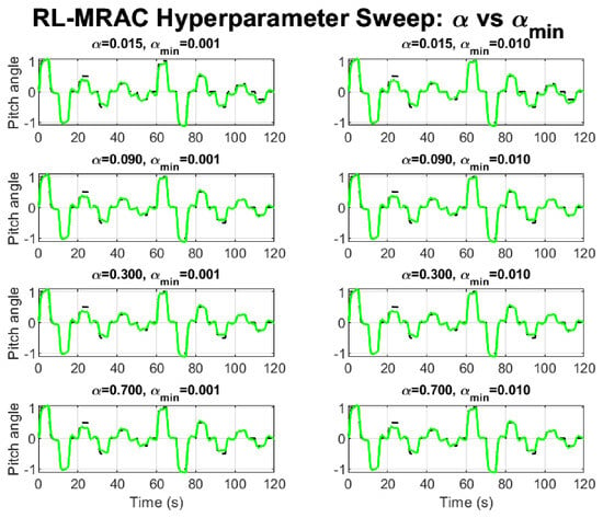
The original learning-rate sweep compared eight pairs of initial and minimum learning rates under S1 with the sinusoidal disturbance. Figure 4 presents the corresponding trajectories, and Table 3 retains the recorded single-run metrics.
Figure 4.
RL-MRAC pitch responses for the eight original learning-rate settings under S1 with sinusoidal disturbance. The green curve shows the RL-MRAC pitch response; the dashed black curve shows the reference-model response.
Table 3.
Original learning-rate sweep: single-run reference-model pitch-error metrics.
The pair , gives the lowest recorded RMSE, P95, IAE, and ITAE among these eight tested settings. It is retained for both square-wave disturbance experiments without pulse-specific retuning. This is a selection within the original single-run sweep, not a claim of globally optimal learning rates or stochastic robustness.
3.4.2. S1 Tracking Without Disturbance
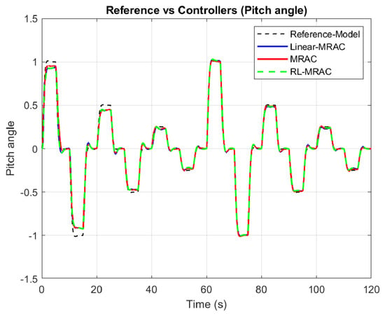
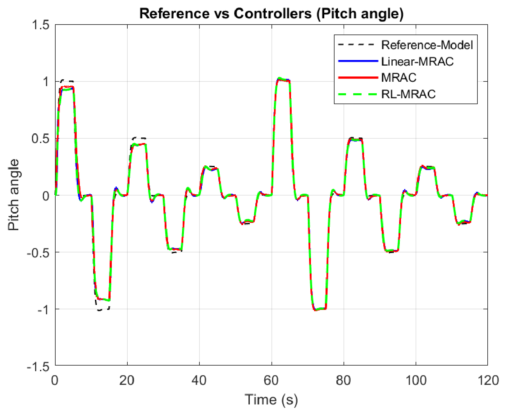
The first S1 case has no additive disturbance. Figure 5 shows the plant responses, reference-model trajectory, and command. The nonlinear MRAC benefits from its supplied regressor basis. The comparison examines the overshoot after switching and the remaining plateau errors.
Figure 5.
Pitch responses of the three primary controllers under S1 without disturbance, seed 42.
Table 4 reports the reference-model pitch-error metrics. Nonlinear MRAC has the lowest reference-model RMSE, IAE, and ITAE in this run. RL-MRAC reduces RMSE from to rad and IAE from to relative to Linear-MRAC, while remaining less accurate than nonlinear MRAC on these measures. Thus, the learned residual provides a modest single-run correction without removing the advantage of structural information in this case.
Table 4.
Single-run reference-model pitch-error metrics, seed 42, S1 without disturbance.
3.4.3. Tracking with Sinusoidal Disturbance
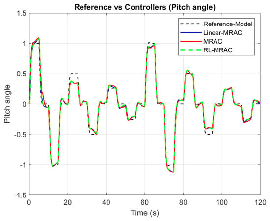
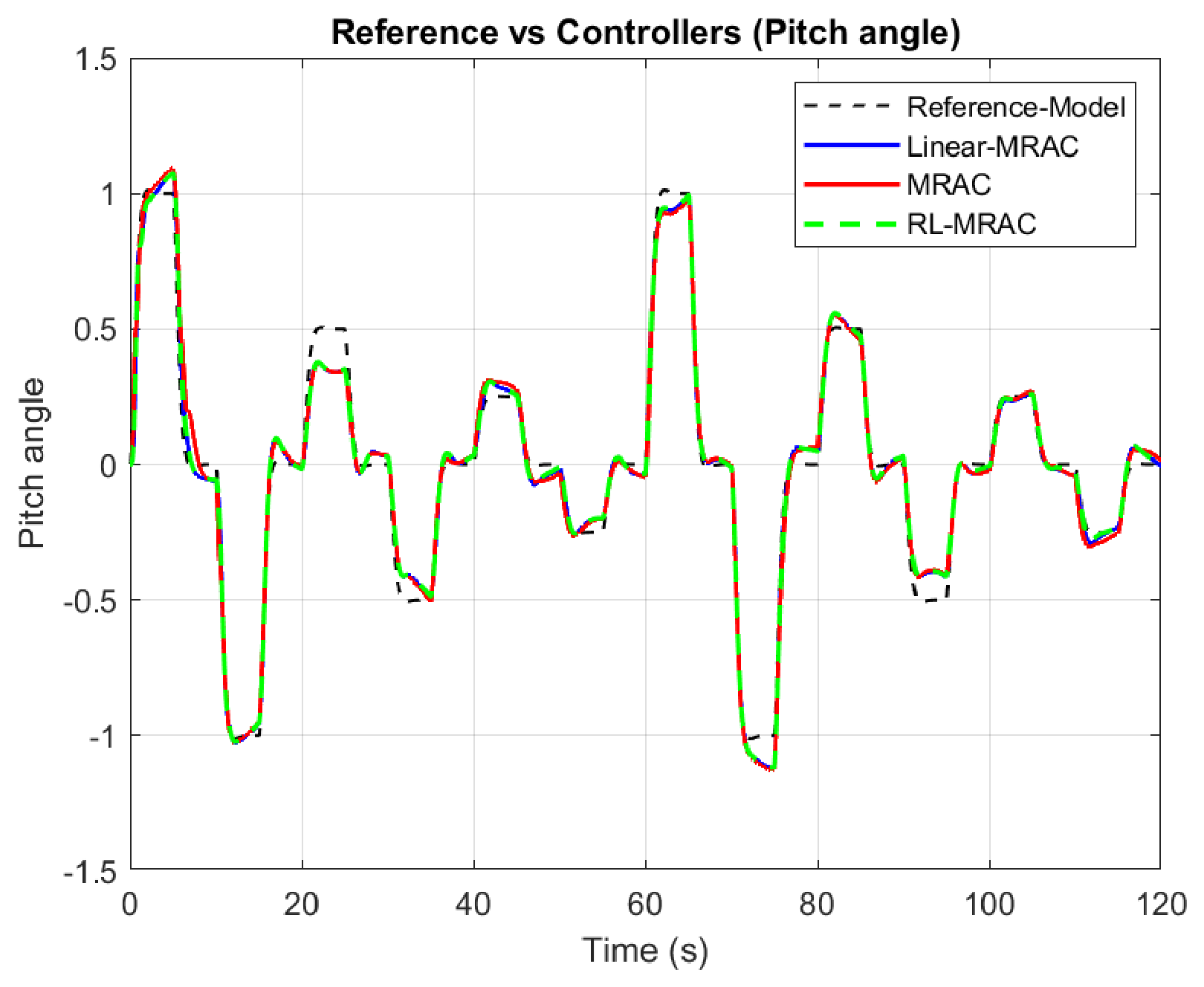
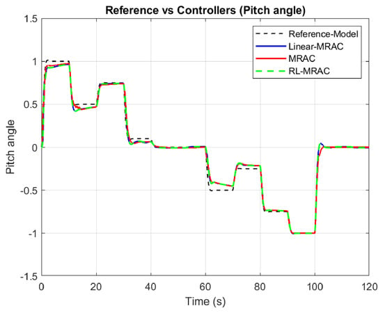
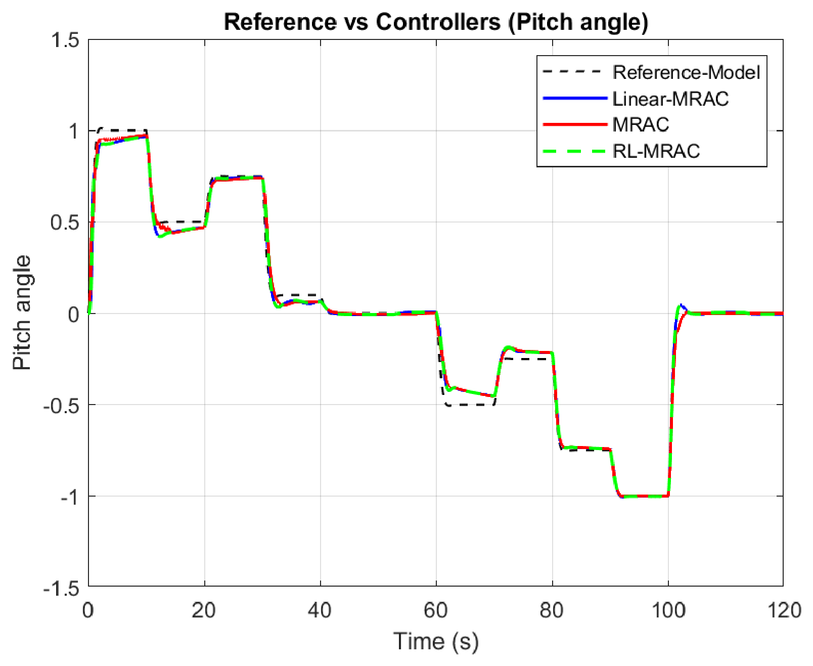
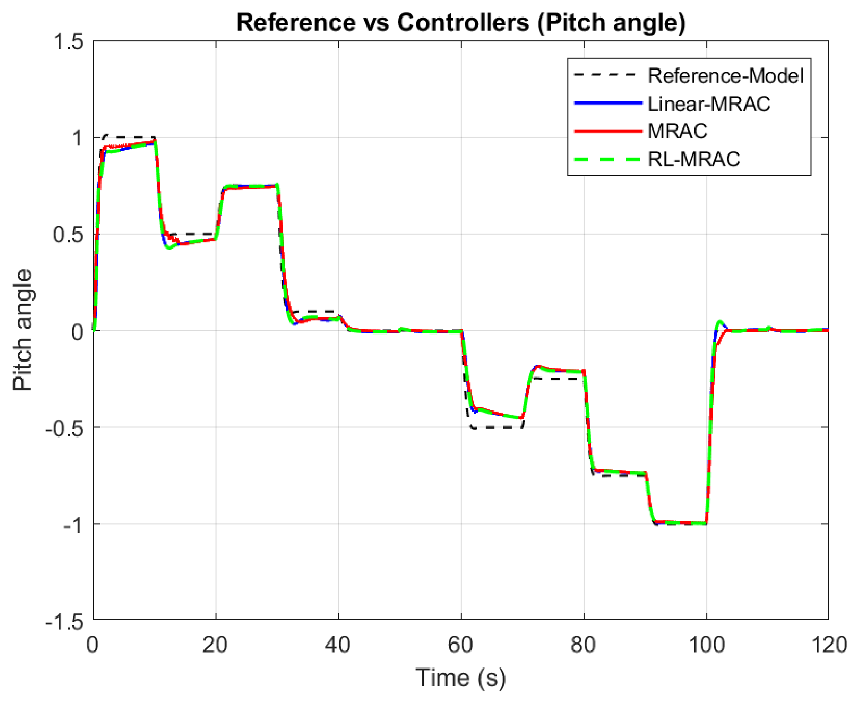
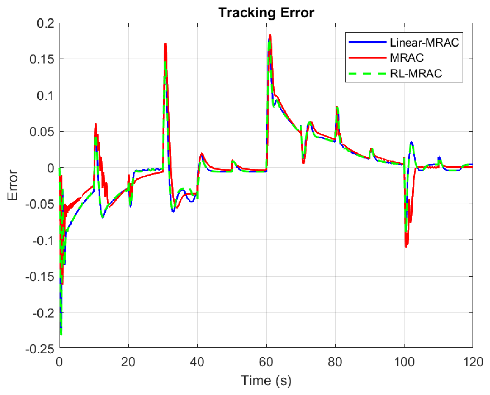
The second S1 case retains the same command and introduces through the numerical disturbance routing specified in Section 3.2. The tracking and error histories are shown in Figure 6 and Figure 7.
Figure 6.
Pitch responses of the three primary controllers under S1 with sinusoidal disturbance, seed 42.
Figure 7.
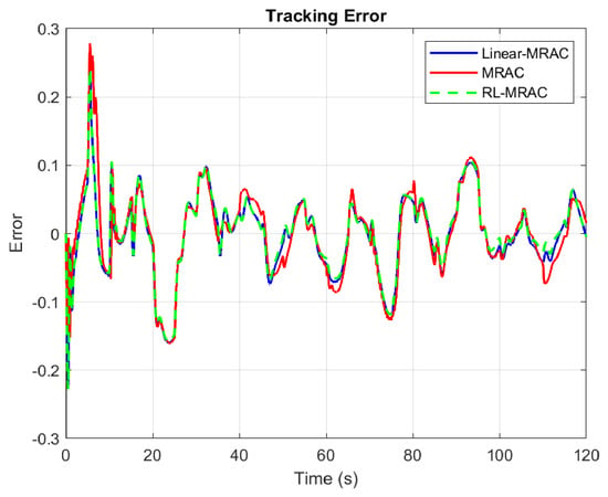
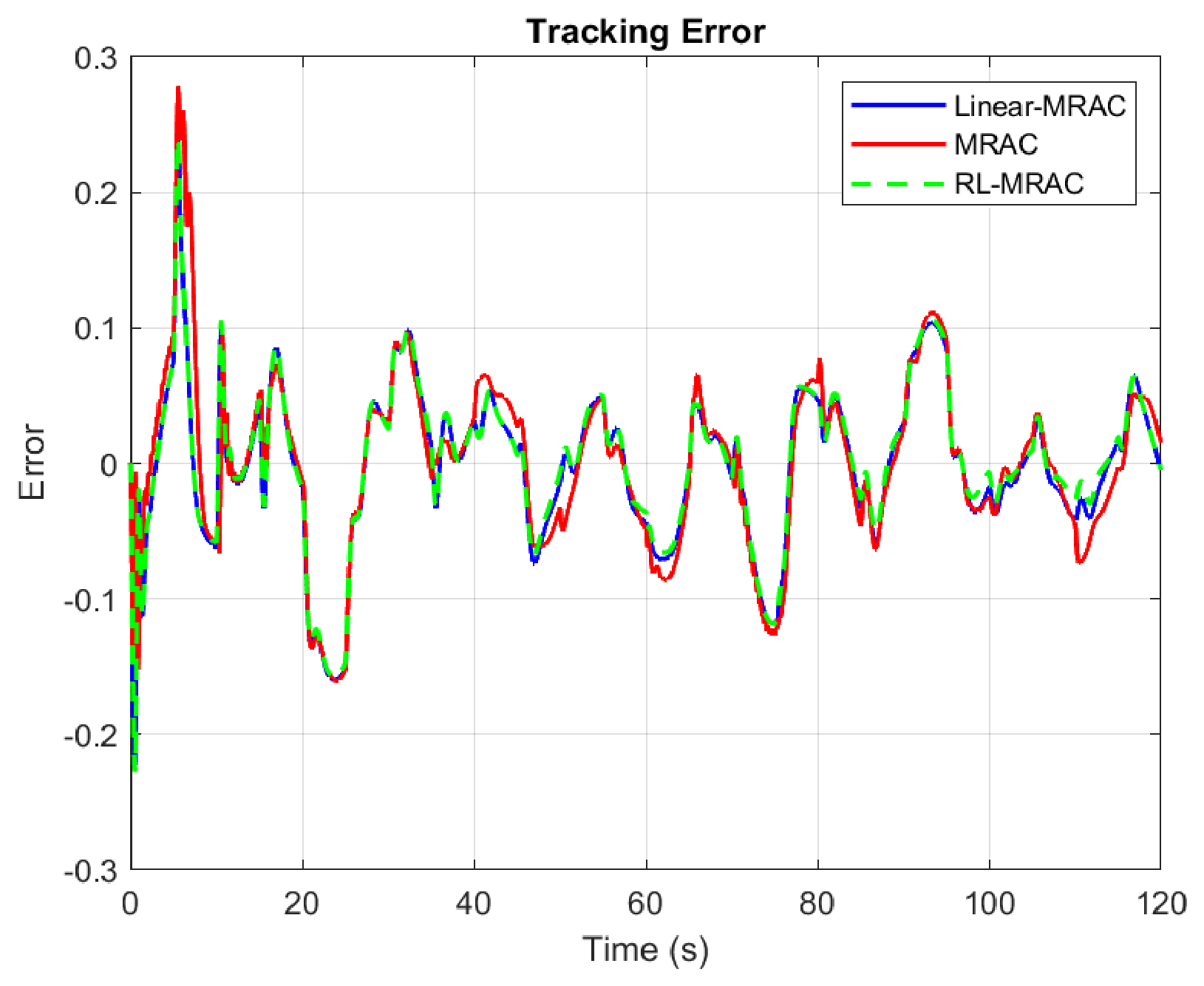
Reference-model pitch errors under S1 with sinusoidal disturbance, seed 42.
In Table 5, RL-MRAC achieves the lowest reference-model error indices among the three primary controllers in this representative run. Its IAE is , compared with for Linear-MRAC and for nonlinear MRAC; ITAE is , compared with and . Relative to Linear-MRAC, these are reductions of approximately and . This preserves the original single-run disturbance-rejection observation. It is not a statement that the same improvement occurs for every initialization or for command RMSE.
Table 5.
Single-run reference-model pitch-error metrics, seed 42, S1 with sinusoidal disturbance.
3.4.4. Nonlinear Compensation and Total Control Input
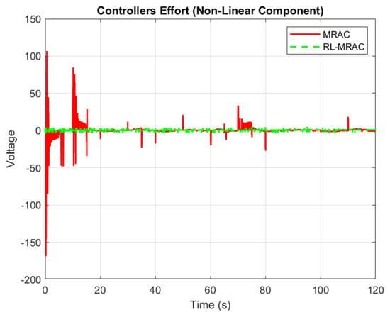
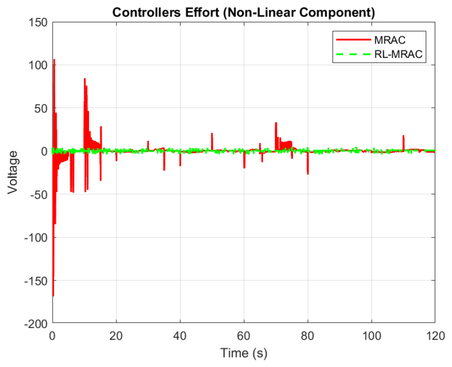
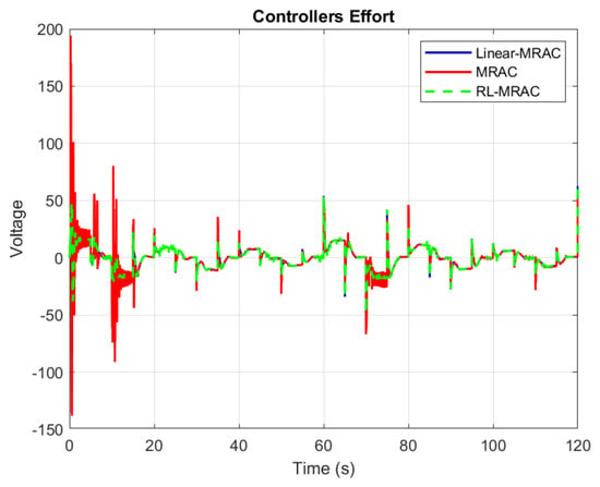
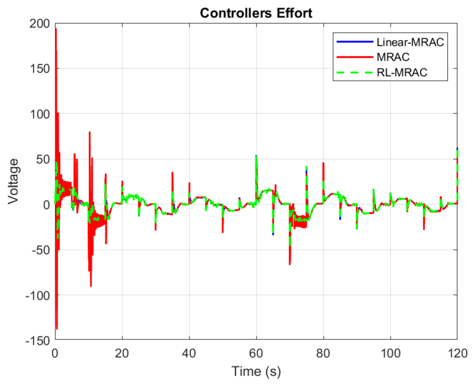
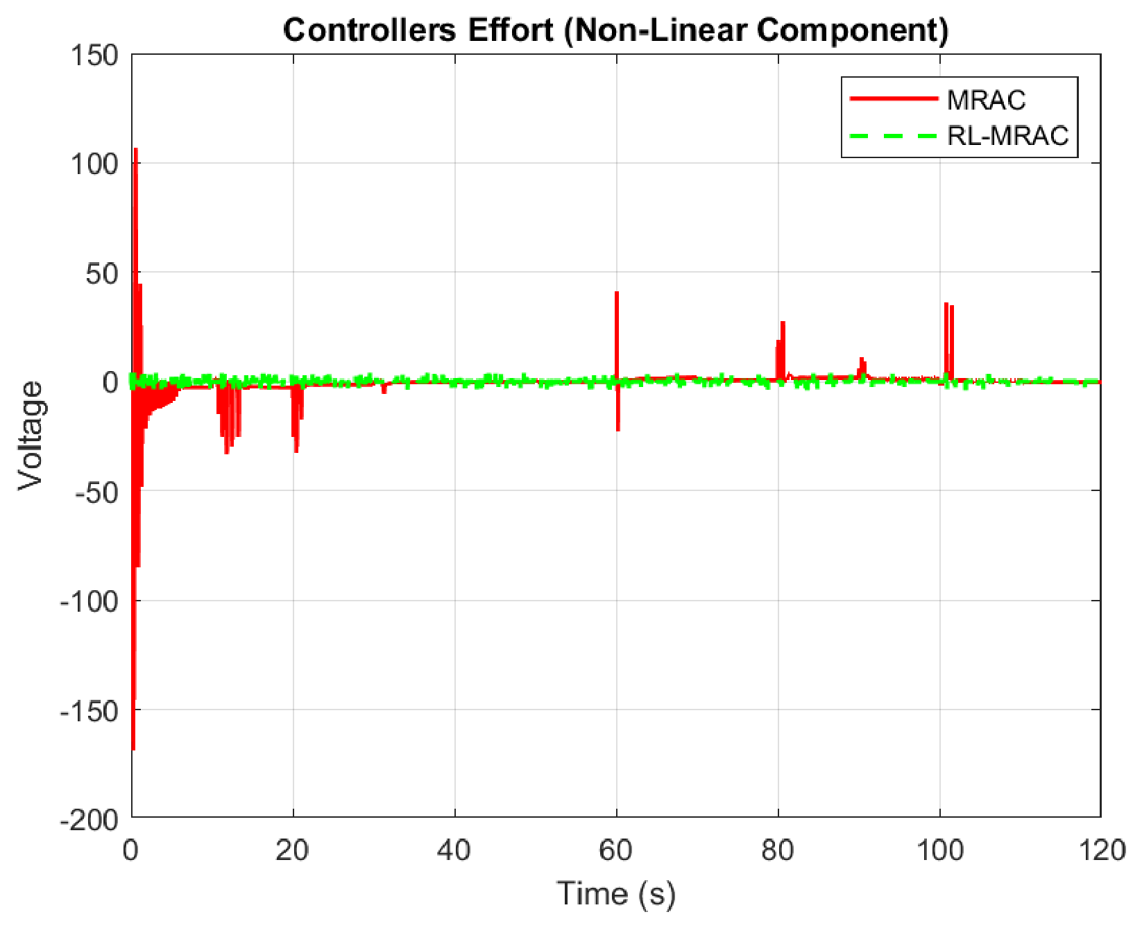
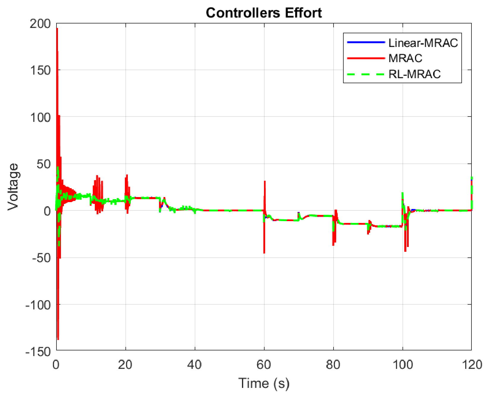
The nonlinear compensation and the RL residual are distinct from the total input. The nonlinear-MRAC term is subtracted from its adaptive baseline; the RL correction is added after the signed gate. Figure 8 shows the original nonlinear-MRAC compensation and selected RL action. The selected action is plotted before the gate; the figure does not separately show the applied residual. The applied residual remains within , but the total inputs in Figure 9 are not constrained by that interval. The histories illustrate when corrections occur; they do not by themselves attribute the tracking difference to regressor delay or establish actuator feasibility.
Figure 8.
Nonlinear-MRAC compensation and selected RL residual under S1 with sinusoidal disturbance.
Figure 9.
Total control inputs of the three primary controllers under S1 with sinusoidal disturbance, seed 42.
3.4.5. Reward and Weight Evolution for S1
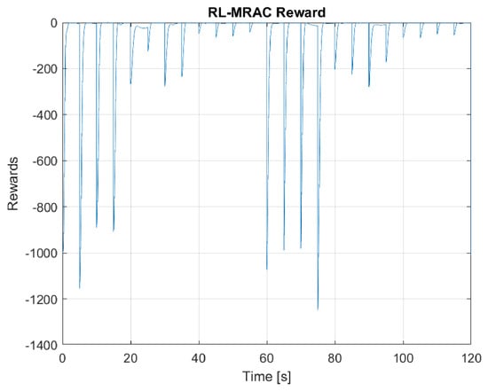
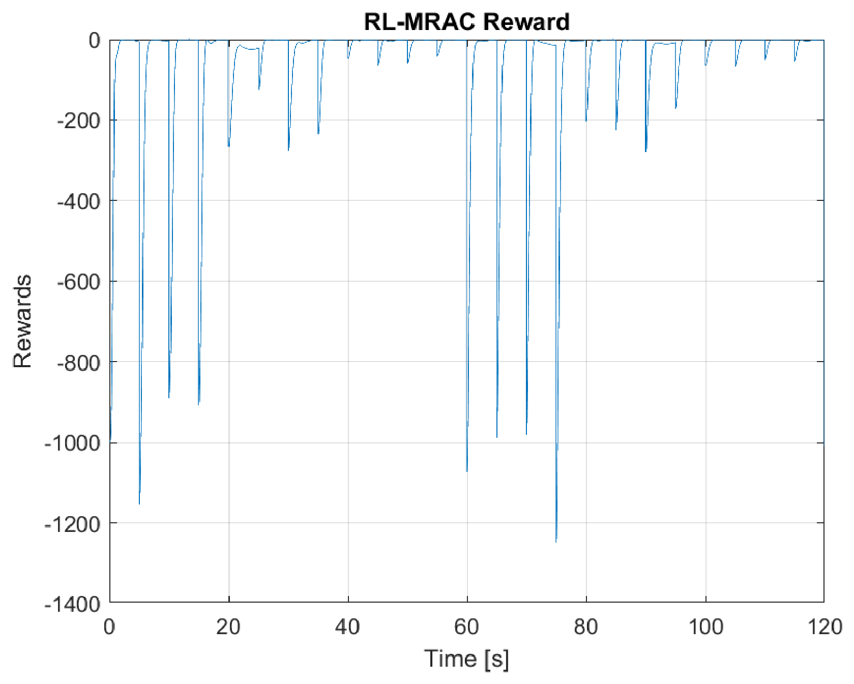
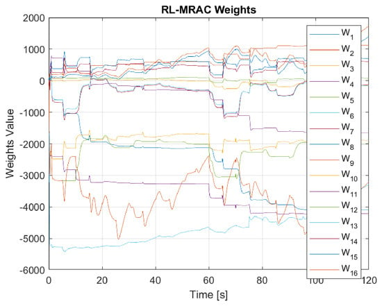
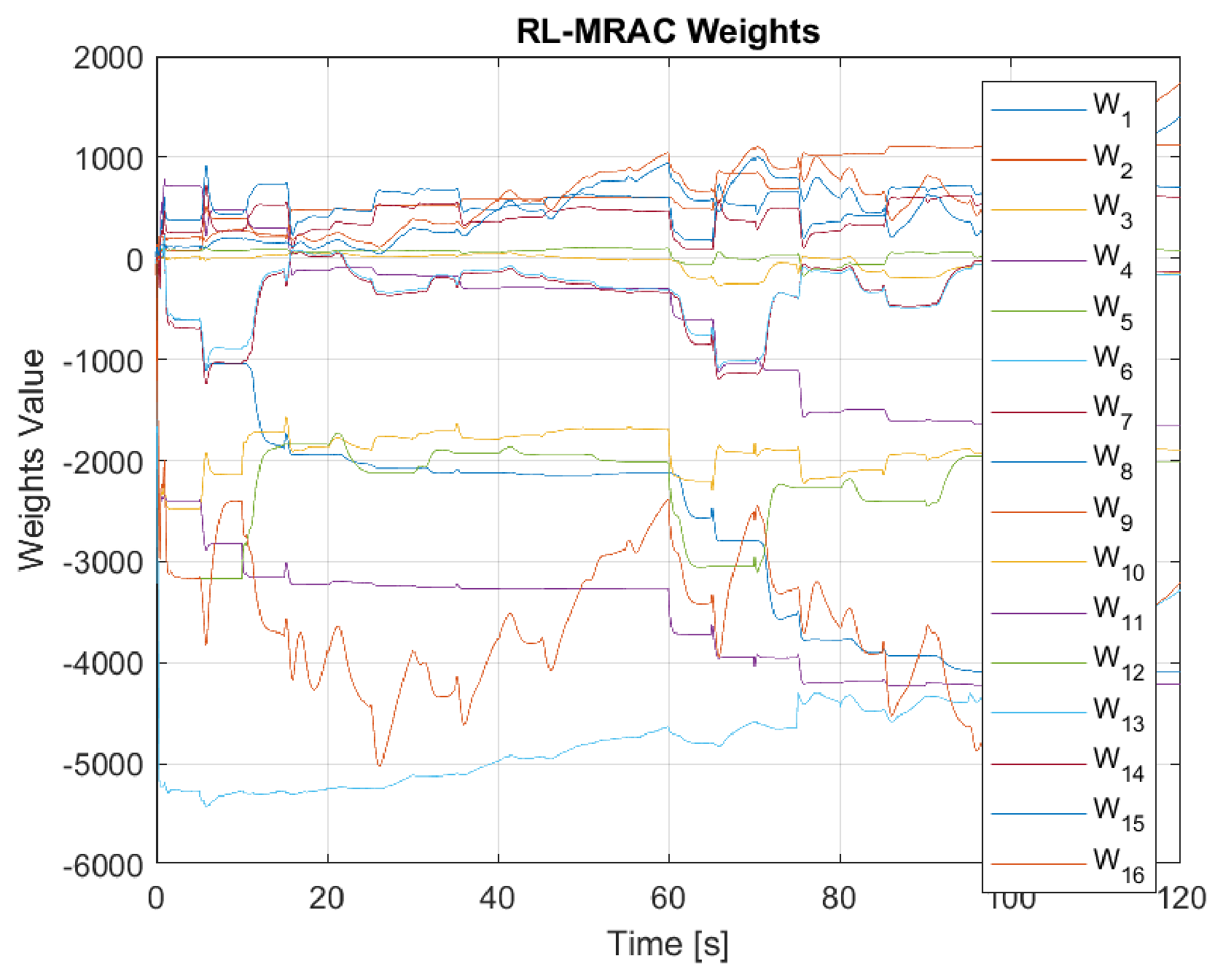
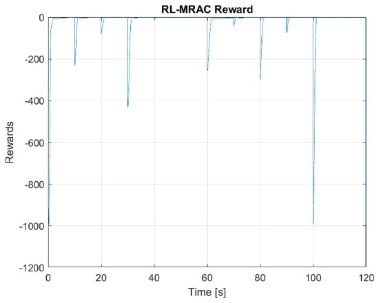
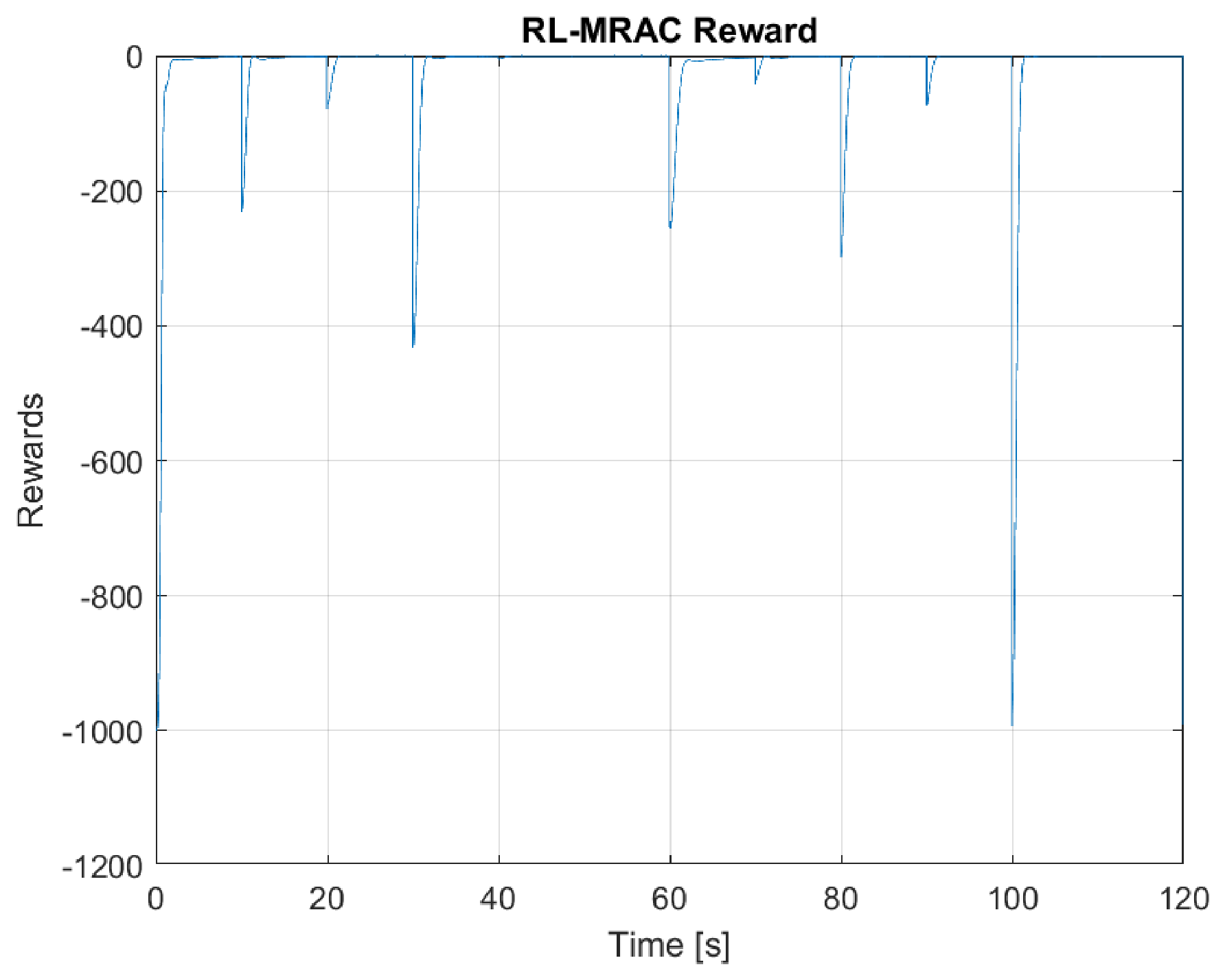
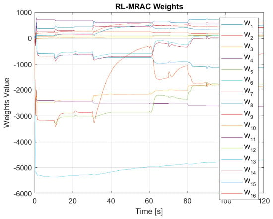
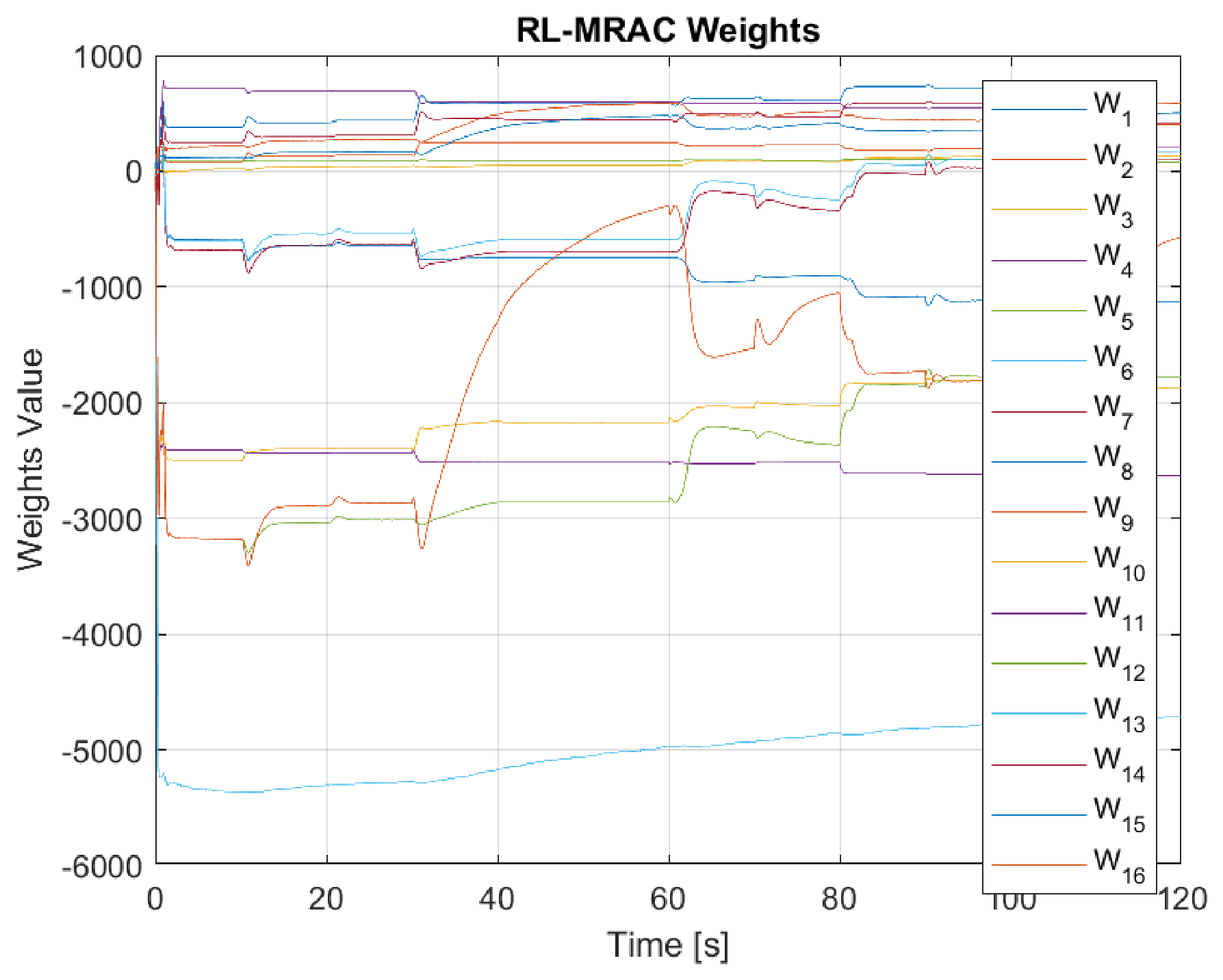
Figure 10 and Figure 11 show the S1 reward and weight histories, respectively. The reward penalizes command error, selected residual magnitude, and the rate-channel state. Its transients reflect repeated command changes and the continuing disturbance. The 16 weights remain finite over the recorded horizon but need not settle to constants. These histories describe the online learning process; they do not prove weight convergence or infinite-horizon adaptive-parameter boundedness. The plant-side tracking analysis uses the applied residual bound and its other stated assumptions.
Figure 10.
RL-MRAC reward history under S1 with sinusoidal disturbance, seed 42.
Figure 11.
Evolution of the 16 TD weights under S1 with sinusoidal disturbance, seed 42.
3.5. Multilevel Square-Wave Tracking with and Without Pulse Disturbance
The second primary experiment uses S2, retaining the same square-wave learning and adaptation settings. It compares a disturbance-free trajectory with the original pulse configuration of amplitude 1, period 10 s, and nominal duration s, beginning at 10 s. For Linear-MRAC, reference-model RMSE is rad with pulses and rad without them. This pulse configuration does not produce a clear RMSE degradation for that baseline.
3.5.1. S2 Tracking Without Disturbance
Figure 12 shows the disturbance-free pitch responses, and Table 6 reports the corresponding reference-model pitch-error metrics. Nonlinear MRAC gives the lowest RMSE and IAE in this run. RL-MRAC gives slightly lower RMSE and IAE than Linear-MRAC and the lowest ITAE of the three. The ITAE ordering differs from the RMSE ordering because later errors receive more weight. A single ordering across every metric is, therefore, not imposed on this case.
Figure 12.
Pitch responses of the three primary controllers under S2 without disturbance, seed 42.
Table 6.
Single-run reference-model pitch-error metrics, seed 42, S2 without disturbance.
3.5.2. Tracking with Periodic Pulses
Figure 13 and Figure 14 show the pulse-case responses and reference-model errors, respectively. In Table 7, RL-MRAC gives the lowest ITAE, , compared with for Linear-MRAC and for nonlinear MRAC. Nonlinear MRAC gives the lowest RMSE and IAE, with RL-MRAC close in RMSE. RL-MRAC improves all four listed model-error indices relative to Linear-MRAC in this run, but it does not dominate nonlinear MRAC across all indices. The pulse experiment demonstrates a transient-performance trade-off for the recorded signal rather than a universal disturbance-rejection ranking.
Figure 13.
Pitch responses of the three primary controllers under S2 with periodic pulses, seed 42.
Figure 14.
Reference-model pitch errors under S2 with periodic pulses, seed 42.
Table 7.
Single-run reference-model pitch-error metrics, seed 42, S2 with periodic pulses.
3.5.3. Compensation and Control Effort
Figure 15 shows the compensation histories, and Figure 16 shows the total control inputs. The compensation histories show different corrective responses around command transitions and pulse events. The RL action bound is respected, whereas total control is governed by the adaptive baseline as well as the residual. Consequently, a bounded learned correction does not establish smoothness or saturation avoidance of the full actuator command. The additional actuator and total-variation studies below examine those questions separately.
Figure 15.
Nonlinear-MRAC compensation and selected RL residual under S2 with pulses.
Figure 16.
Total control inputs of the three primary controllers under S2 with pulses, seed 42.
3.5.4. Reward and Weight Evolution for S2
Figure 17 and Figure 18 show the reward and weight histories, respectively, for the pulse experiment. Weight values remain finite over the 120 s record, but convergence is not claimed. These traces support a finite-horizon implementation assessment; they do not replace the conditional assumptions in Section 2.8 or the repeated-seed evaluation that follows.
Figure 17.
RL-MRAC reward history under S2 with periodic pulses, seed 42.
Figure 18.
Evolution of the 16 TD weights under S2 with periodic pulses, seed 42.
4. Additional Validation and Sensitivity Studies
The primary single-run experiments above remain the central time-domain comparison. This section adds the independent learning-based baseline, seed ensemble, and robustness and sensitivity evidence. The additional tests qualify the scope of the primary observations; they do not replace the representative tracking, control, reward, and weight histories.
4.1. Additional RBF-NN MRAC Baseline
An online radial-basis-function neural MRAC controller is added as a transparent adaptive-learning comparator, not as a claim to cover all state-of-the-art methods. It uses the same Linear-MRAC backbone and subtracts :
The 25 Gaussian centers form a grid over pitch and rate , with widths and 1, respectively. A bias gives 26 features, normalized by their Euclidean norm plus . Neural estimates start at zero and their gain is not retuned by case. This controller receives measured states but no true plant nonlinear basis. It shares all plant, disturbance, and actuator settings in each comparison. The conditional proof for the original three architectures is not asserted to establish a separate theorem for this additional neural baseline.
4.2. Representative Four-Controller Responses
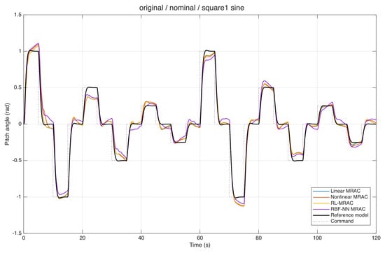
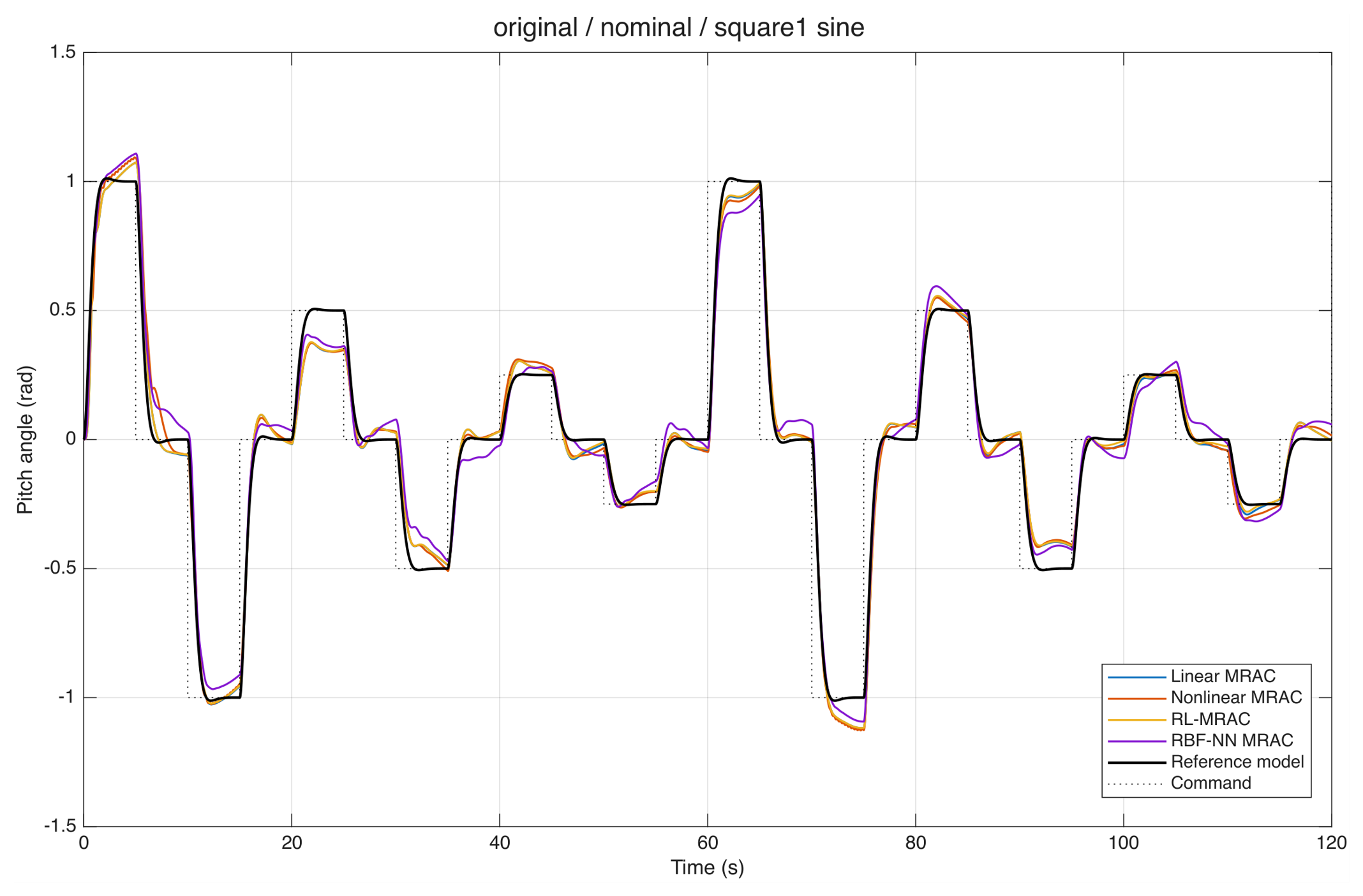
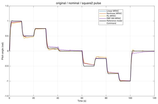
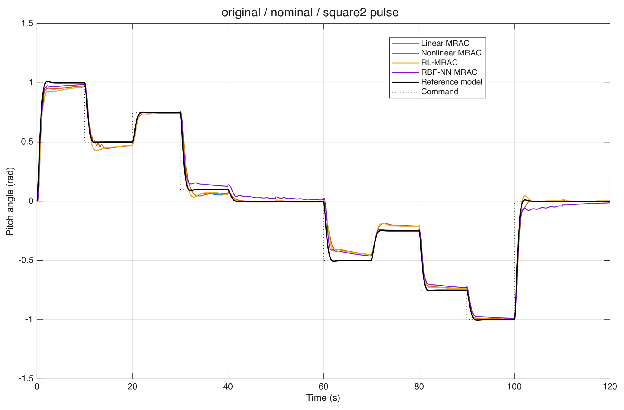
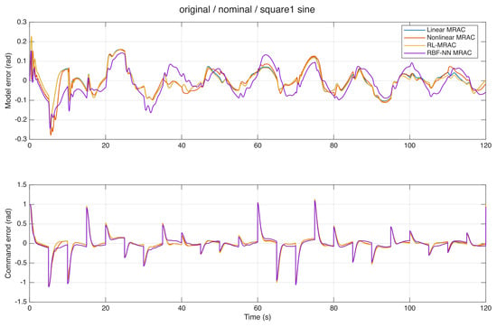
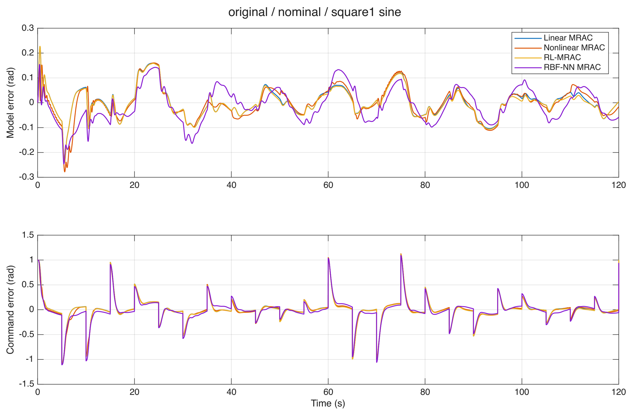
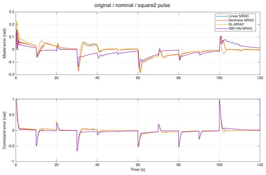
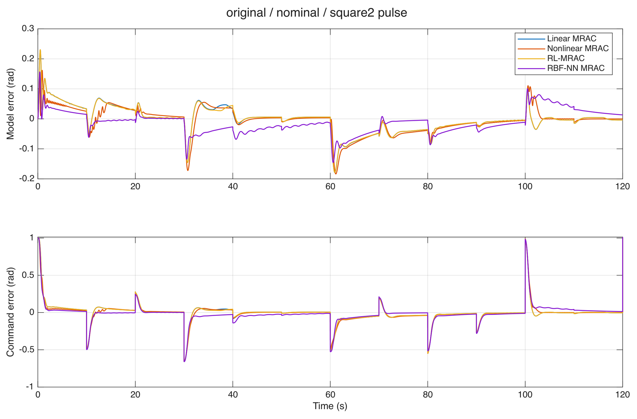
Figure 19 and Figure 20 compare the pitch responses of the three primary controllers and the RBF-NN MRAC baseline for S1 and S2, respectively. Figure 21 and Figure 22 show the corresponding reference-model and command-tracking errors. These additional validation runs are distinct from the original-submission three-controller histories above.
Figure 19.
Pitch responses of the four controllers, command, and reference model under S1 with sinusoidal disturbance (seed 42).
Figure 20.
Pitch responses of the four controllers, command, and reference model under S2 with periodic pulses (seed 42).
Figure 21.
Reference-model and command errors for the four controllers under S1 with sinusoidal disturbance (seed 42).
Figure 22.
Reference-model and command errors for the four controllers under S2 with periodic pulses (seed 42).
4.3. Twenty-Seed Controller Comparison
Seed 42 was also used to select the learning rates in the S1 sinusoidal case and is included in the ensemble; the ensemble is not a held-out tuning validation. Its reference-model RMSE is 1.4–2.6 sample standard deviations below the corresponding RL-MRAC mean in all four principal cases. All 320 controller trajectories in the four principal 20-seed cases completed successfully. Table 8 reports command tracking, and Table 9 reports reference-model tracking. The mean RL-MRAC reference-model RMSE is slightly higher than that of Linear-MRAC in both S2 cases. Deterministic baselines have zero seed variability in these noise-free cases; repeating them provides a matched comparator for each stochastic RL realization, not additional independent baseline evidence.
Table 8.
Command-tracking metrics over 20 seeds. Values are mean ± sample standard deviation; zero variation is omitted. RMSE is in rad, IAE in rad s, and ITAE in rad s2.
Table 9.
Reference-model pitch RMSE (rad) over 20 seeds, separately from command RMSE.
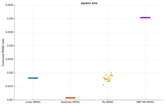
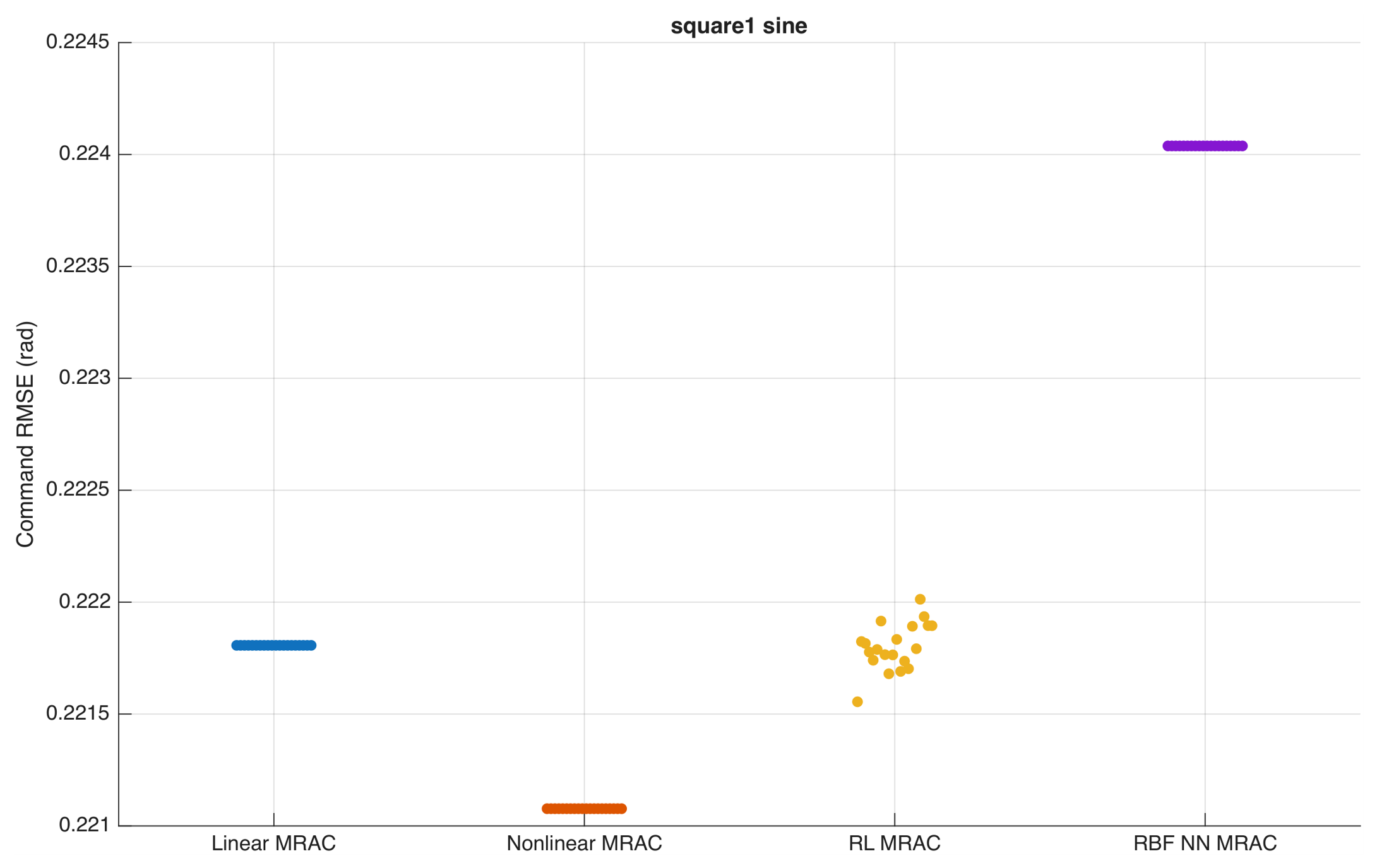
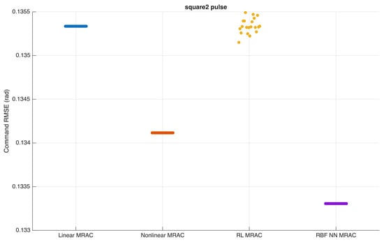
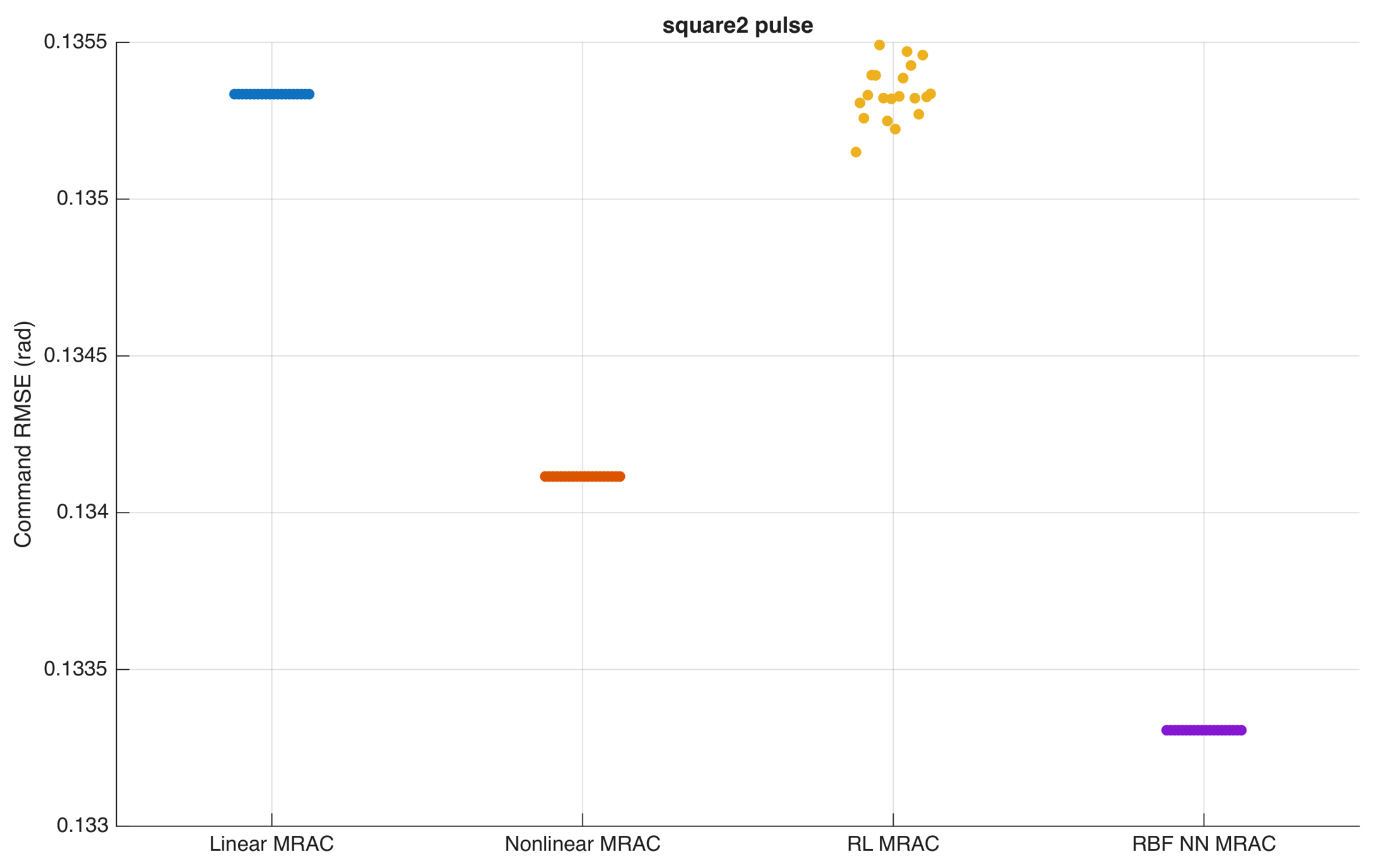
Figure 23 and Figure 24 show the per-seed results for S1 with sinusoidal disturbance and S2 with periodic pulses, respectively. RL-MRAC and Linear-MRAC have nearly identical mean command RMSE. In S1 with the sinusoid, their values are and rad; in S2 with pulses, they are and rad. The paired bootstrap intervals for their command-RMSE differences include zero in all four cases, and the Holm-adjusted sign-test values equal 1. This does not establish equivalence, but it does not support a consistent improvement claim. RL-MRAC also has higher total input variation than Linear-MRAC in every main case.
Figure 23.
Per-seed command RMSE under S1 with sinusoidal disturbance; 20 seeds per controller.
Figure 24.
Per-seed command RMSE under S2 with periodic pulses; 20 seeds per controller.
Rankings depend on the error definition and metric. Under the S1 sinusoid, nonlinear MRAC has lower command RMSE than RL-MRAC, whereas RL-MRAC has lower reference-model RMSE and lower command IAE/ITAE. The RBF-NN baseline has the lowest command RMSE in both S2 cases, while nonlinear MRAC has the lowest in S1 without disturbance and S1 with the sinusoid. Therefore, the earlier claim that RL-MRAC is uniformly best under disturbances is replaced by a metric-specific comparison.
4.4. Coefficient and Learning-Design Sensitivity
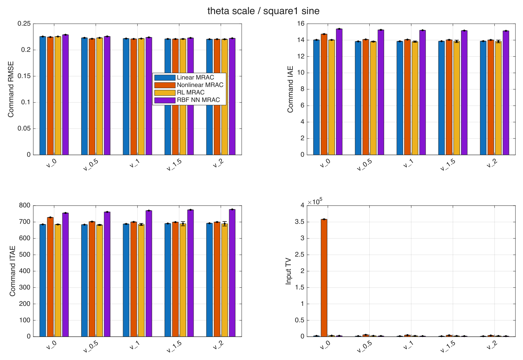
Joint coefficient scaling changes the ranking (Figure 25). For S1 with the sinusoid, at scale 1 the five-seed mean command RMSE is for nonlinear MRAC and for RL-MRAC; at scale 2 it is and , respectively. For S2 with pulses, the RBF-NN baseline improves from at zero nonlinear coefficients to at scale 2. The joint and individual-coefficient sweeps, therefore, do not support a ranking invariant to synthetic nonlinearity magnitude. Table S2 reports the individual-coefficient sweeps. At zero scale, nonlinear MRAC still adapts its compensation and its mean input TV rises to about V. The available results establish the increase, but do not isolate its cause.
Figure 25.
Coefficient-scale sensitivity under S1 with sinusoidal disturbance; five seeds per setting.
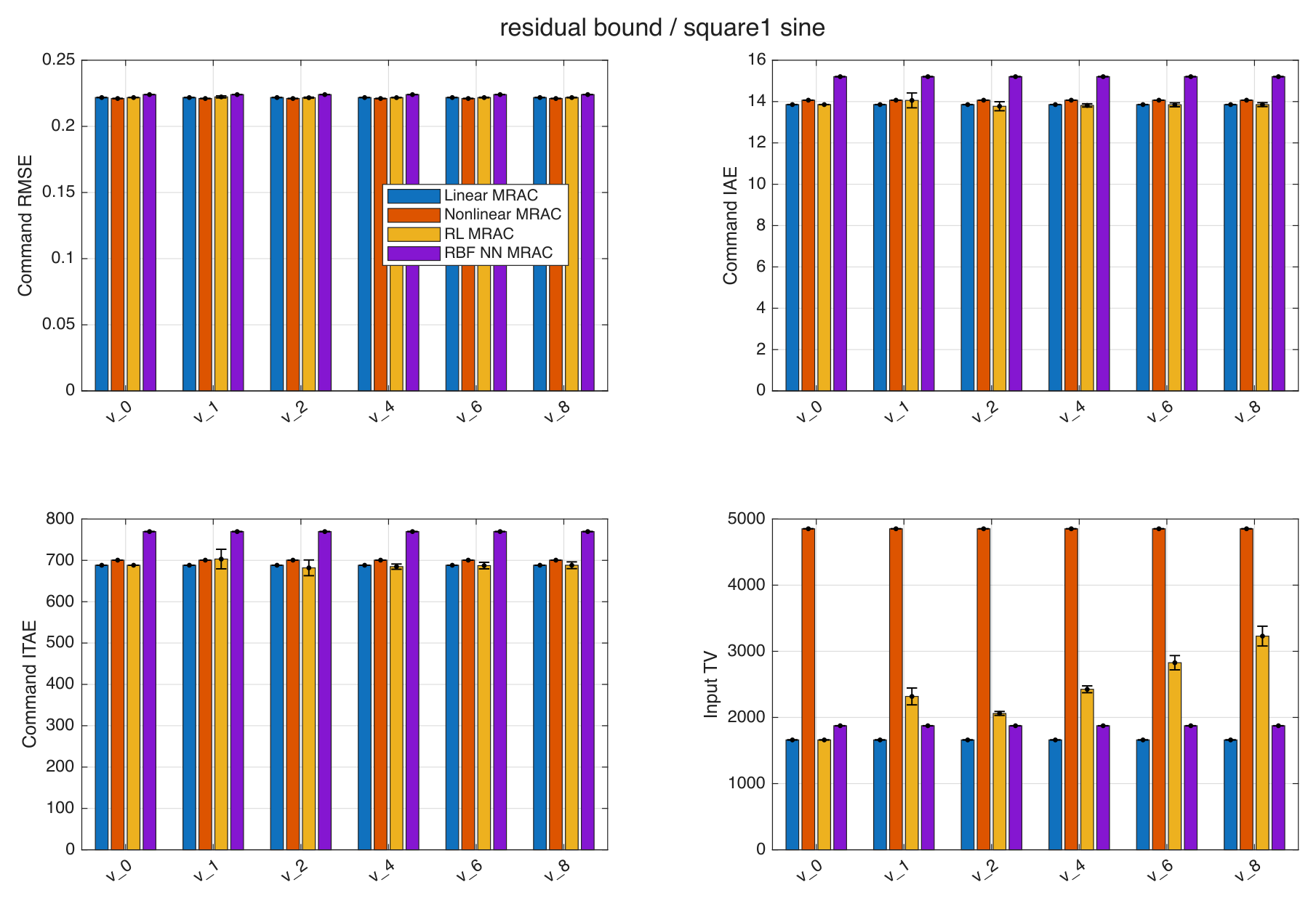
The residual bound is swept over (Figure 26). For a symmetric actuator range , select from available headroom: is a sufficient amplitude check if the baseline demand bound holds over the intended operating envelope. This does not enforce slew limits. With other constants fixed, increasing increases the derivative-negativity threshold at rate ; the ultimate tracking radius follows separately from the Lyapunov level set. Because the measured tracking response is nonmonotonic, choose feasible headroom first and tune within it empirically. A zero bound recovers the Linear-MRAC plant input. Mean command error is not monotonic in the bound: for S1 with the sinusoid, RL-MRAC RMSE is at bound 1, at bound 2, and at bound 4. Thus, 4 remains an empirical nominal choice rather than a demonstrated optimum. Increasing the bound also enlarges the conservative analytical tracking bound when the other bounding constants are fixed, as derived in Section 2.8.
Figure 26.
Residual-bound sensitivity under S1 with sinusoidal disturbance; five seeds per setting.
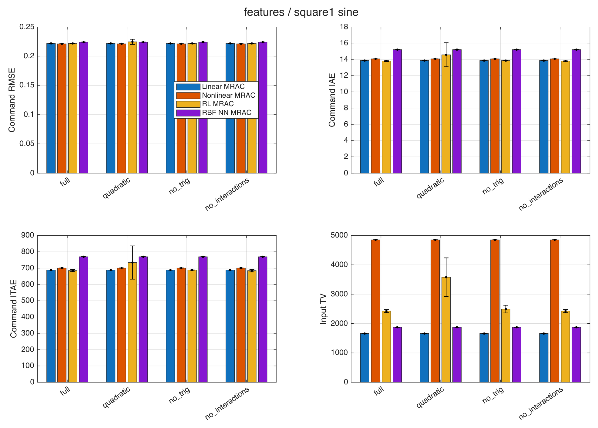
Exploration rates , discount factors , and action counts are evaluated separately. Action-resolution changes produce small mean differences in these cases and do not establish that 1000 actions are necessary. Figure 27 compares the feature dictionaries. Table S2 reports the exploration and action-resolution results, as well as the discount, feature, and gate comparisons. Discount changes can be more consequential: for S2 with pulses, gives mean command RMSE with SD , compared with with SD at .
Figure 27.
Feature-dictionary ablation under S1 with sinusoidal disturbance; five seeds per dictionary.
Feature ablation compares the full dictionary, a quadratic subset, removal of trigonometric features, and removal of state–action interactions. Under S1 with the sinusoid, the quadratic subset gives RMSE , compared with for the full dictionary; removing trigonometric terms gives . Under S2 with pulses, removing trigonometric terms slightly lowers the mean from to . These results support examining dictionary size but do not establish the necessity of every term. Gate ablation likewise tests the preserved signed gate against no gate and an absolute-error gate; it does not convert the evaluated learner into conventional SARSA.
4.5. Noise, Irregular Disturbances, and Actuator Stress
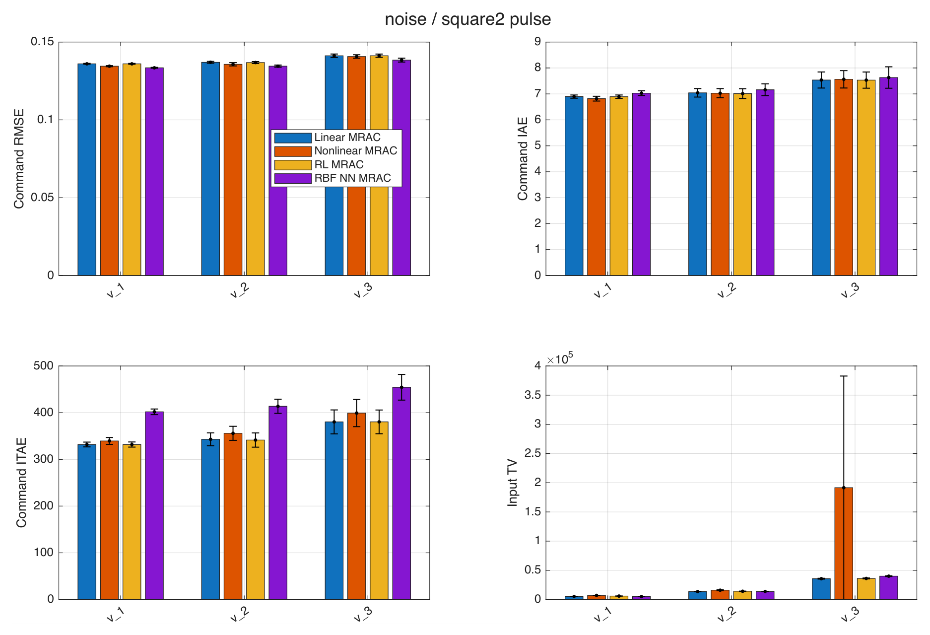
Figure 28 summarizes the S2 measurement-noise tests. Sampled Gaussian measurement noise is shared across controllers, with angle/rate standard-deviation pairs , , and in rad and rad/s. The highest level increases S2-pulse mean command RMSE to , , , and for Linear-MRAC, nonlinear MRAC, RL-MRAC, and RBF-NN MRAC, respectively. This is a measured degradation, not evidence that noise sensitivity is eliminated.
Figure 28.
Measurement-noise sensitivity under S2 with pulses; five seeds per noise level.
Irregular disturbances combine a filtered Gaussian scalar signal with correlation time s and stationary standard deviation , and three localized gust-like pulses. They use the same numerical routing as the main disturbances and are not calibrated wind-speed or aerodynamic-torque models. RL-MRAC and Linear-MRAC again have close mean command errors: versus for S1 and versus for S2. A separate parameter-change test increases all nonlinear coefficients by 50% and inertia by 25% at 60 s. Gaussian inputs have unbounded support, so these finite-run tests do not verify the bounded-disturbance assumptions of the theorem for all time.
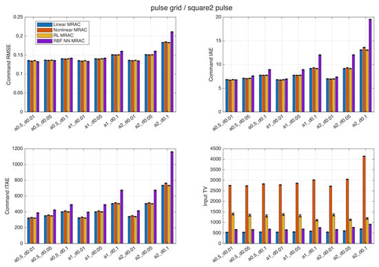
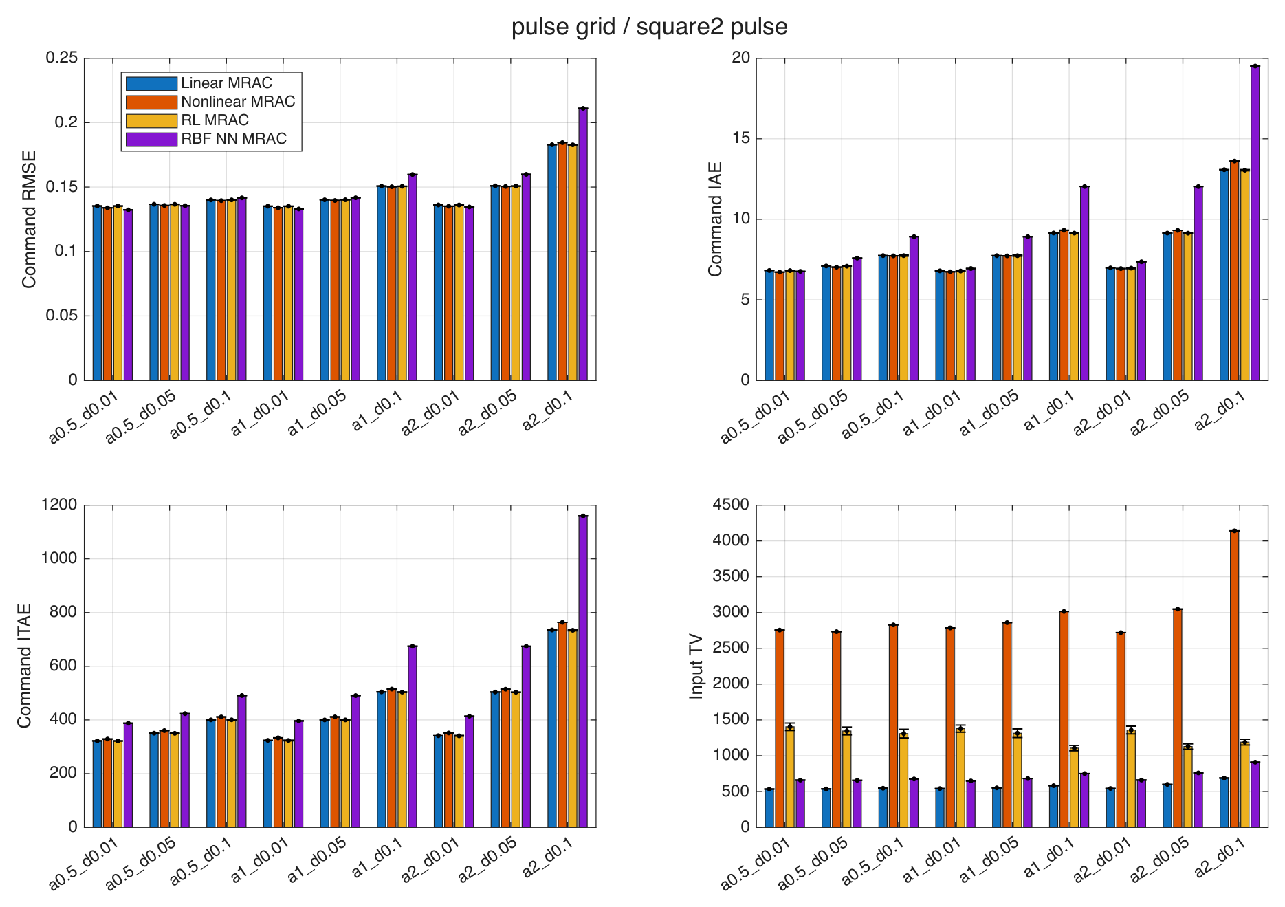
Figure 29 summarizes the pulse grid, which varies amplitude over and duration over s at a fixed 10 s period. For amplitude 2 and duration s, the mean command RMSE is , , , and for the four controllers in the same order. This grid broadens the transient tests but does not characterize pulse-period sensitivity.
Figure 29.
Pulse-amplitude and duration sensitivity under S2; five seeds per setting and a fixed 10 s period.
Actuator uncertainties include gains 0.8 and 1.2, and gain 0.8 with a s first-order lag. In the lagged S1-sinusoid case, nonlinear MRAC meets the numerical termination criterion at s for all five trials; the failure count is retained rather than averaging a truncated response as a completed trajectory. The aggregate study records five failed controller trajectories among 2612 planned trajectories. Table S2 reports the parameter-step and actuator-gain results. At the highest measurement-noise level, nonlinear-MRAC input TV is V on average (sample SD V), indicating substantial variation across the five noise realizations. For nonlinear MRAC the command RMSE is rad at V and rad at V with the same slew limit. The result is nonmonotonic; the tests do not establish whether adaptive gain drift explains it. These numerical failures indicate sensitivity of this implementation, not a general instability theorem for nonlinear MRAC.
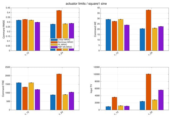
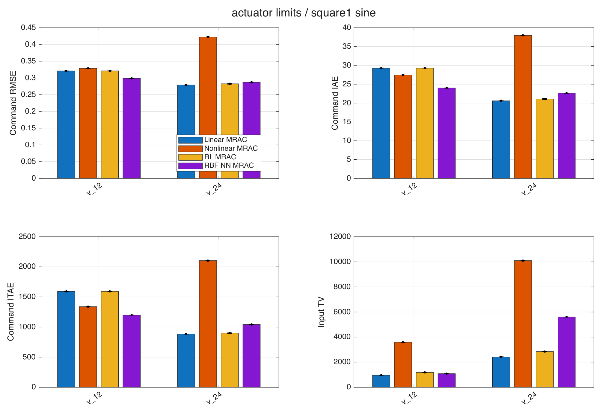
Figure 30 summarizes additional actuator-limit tests that impose hypothetical amplitude bounds of or V and a slew limit of 100 V/s equally on all controllers. At V under S1 with the sinusoid, RL-MRAC mean command RMSE increases to and its amplitude- and slew-limited fractions are and . Linear-MRAC gives , , and . These limiter-activation fractions can overlap. They demonstrate that bounding only the residual does not make the total command actuator-safe.
Figure 30.
Tracking and input-variation metrics with common amplitude and slew limits under S1 with sinusoidal disturbance.
4.6. Separate Nonlinear-Regressor Delay Study
The shared previous-input regressor in the main model does not itself create plant–compensator mismatch. To isolate controller-regressor timing on a common alternative plant, a separate family uses the current applied input in every plant branch and compares nonlinear compensation delays of 0, 1, and 2 samples. The zero-delay controller solves its implicit scalar control equation with a relative residual tolerance of , using the previous input as the initial guess, Newton iterations, and a bracketed fallback. Existence of a numerically accepted root does not establish uniqueness or independence from root selection.
Table 10 reports nonlinear-MRAC command RMSE and the RMS input-equivalent mismatch . No trial in this family fails. Removing the delay does not improve tracking in these tests: the zero-delay RMSE is higher than the one-sample value in both cases. Hence, poorer performance in a selected original-submission comparison cannot be explained simply by asserting a harmful one-sample regressor delay. The results apply to this separate current-input model and the implemented numerical root selection. Implicit root selection and the coupling through the input-dependent nonlinear terms are possible explanations for the observed ranking, but their separate effects were not isolated.
Table 10.
Nonlinear-MRAC delay comparison on the separate current-input plant; three seeds per case. Mismatch is in input-equivalent units.
4.7. Additional Transient and Control Measures
Settling time is measured after each nonzero command transition using a band that must hold for the remaining dwell interval. A transition that never satisfies this requirement is marked nonsettled, not assigned zero settling time. Overshoot is directional excess beyond the new command divided by the transition magnitude. Consequently, persistent disturbances can leave some or all transitions without a finite settling time, and medians conditional on settled segments should be interpreted with the settled/total counts. Table S1 reports these counts alongside settling time, overshoot, peak and P95 command error, and mean input variation. Table S3 reports the step, sine, and ramp reference cases.
For S1 with the sinusoid, RL-MRAC mean input total variation is V, compared with V for Linear-MRAC. For S2 with pulses, the corresponding values are and V. The added learning correction, therefore, increases sample-to-sample control variation despite the similar tracking means. Main-case total input peaks also exceed the additional V stress limit; no hardware voltage constraint is assumed in those unconstrained cases.
A supplementary step-size comparison uses and s. Changing this step also changes action-selection timing, discrete delays, and learning evaluations per unit time, so it is a combined implementation sensitivity test rather than a pure numerical convergence proof at fixed controller timing.
4.8. Computational Requirements
Host measurements use an Apple M4 computer, MATLAB R2025b Update 1 (25.2.0.3042426), MACA64, and Apple Accelerate BLAS (ILP64). Each warmed-up benchmark is repeated 300 times using the terminal state and weights of the nominal S1-sinusoid trial. One greedy search scores normalized 16-feature vectors, giving scoring complexity. An individual semi-gradient update is , excluding action selection.
Table 11 reports results for 1000 actions. The learning-cycle kernel includes two greedy searches and four TD evaluations; it must not be described as the cost of a single weight update. The complete numerical-step kernel additionally integrates the reference model and all four controller/plant branches through the three ode3 stages. These benchmarks use representative-state kernels rather than timing a full acquisition-and-control loop. Mean complete-step time is of the 10 ms interval, and no measured repetition exceeds that interval. Hardware I/O, sensing, logging, and full-trajectory storage are excluded. An observed maximum is not a worst-case execution-time guarantee, and the host measurements do not establish embedded real-time feasibility.
Table 11.
Host computation time (ms), 1000 candidate actions, 16 TD features, 300 repetitions.
4.9. Limitations
The results cover finite-horizon simulation of a single pitch axis with synthetic nonlinear coefficients, a clipped basis, and broadcast disturbance routing. Full-state measurement is assumed. Estimating pitch rate in hardware can introduce estimation error and phase lag that affect the adaptive laws, gate, and learner; noisy full-state simulation does not evaluate an observer. Residual clipping does not constrain total voltage or slew, and the host timing excludes sensing, communication, scheduling, and hardware I/O. Quanser experiments, embedded timing, a causal SARSA redesign and robust adaptive-law modifications remain future work. Coupled six-degree-of-freedom flight requires multi-input learning, control allocation, and a new analysis. The evaluation does not establish superiority over GP-MRAC, sliding-mode adaptive control, or other residual RL methods.
5. Conclusions
This work developed and evaluated a bounded residual learning augmentation of Linear-MRAC for nonlinear single-axis tracking. The primary study retains the complete representative comparisons: tracking responses, reference-model errors, compensation components, total control inputs, rewards, weight evolution, and the original learning-rate sweep. In the S1 sinusoidal single run, RL-MRAC gives lower reference-model MSE, RMSE, IAE, and ITAE than the two primary benchmarks, including IAE and ITAE reductions of approximately and relative to Linear-MRAC. In the S2 pulse run, RL-MRAC has the lowest ITAE, while nonlinear MRAC has lower RMSE and IAE. The disturbance-free cases likewise show the importance of both structural information and the selected error index.
The additional RBF-NN baseline, 20-seed ensemble, and sensitivity studies assess how broadly those single-run observations extend. The ensemble does not establish a consistent command-tracking improvement over Linear-MRAC, and residual learning increases input total variation. These findings qualify the generality of the representative results rather than erase their time-domain behavior. Rankings depend on the reference, disturbance, coefficient setting, and whether command error or reference-model error is measured.
The conditional Lyapunov result maps the scalar residual through the input matrix and characterizes ultimate tracking under matching, bounded effective uncertainty, forward completeness, and assumed bounded adaptive parameter errors. It neither proves boundedness of the unmodified gradient estimates under persistent disturbances nor guarantees improvement from a bounded residual. Feature normalization and finite weight traces likewise do not establish convergence of the TD recursion. The implemented buffered target and solver-output updates are explicitly distinguished from conventional forward-transition SARSA.
The noise, irregular-disturbance, parameter-change, pulse-grid, and actuator studies broaden the finite-horizon evidence, while revealing practical limitations. Residual bounds alone do not limit the total input or slew rate. Actuator constraints degrade tracking, and the gain-plus-lag test produces five nonlinear-MRAC numerical failures. Host computation fits within the chosen interval in the measured repetitions, but sensing, communication, scheduling, and embedded worst-case execution remain unvalidated.
Supplementary Materials
The following supporting information can be downloaded at: https://www.mdpi.com/article/10.3390/machines14111380/s1, Table S1: Transient and control measures across the four 20-seed cases; Table S2: Sensitivity, stress, and implementation studies; Table S3: Original step, sine, and ramp reference tests; Dataset S1: Per_Run_Metrics.csv (per-trajectory metrics and completion status).
Author Contributions
A.A.E. contributed to the conceptualization, methodology, software development, validation, investigation, formal analysis, and original manuscript preparation. B.J.E. contributed to the conceptualization, methodology, formal analysis, manuscript review and editing, and research supervision. All authors have read and agreed to the published version of the manuscript.
Funding
This work was supported in part by the American University of Sharjah (AUS), Faculty Start Up Research Grant (FSU) Program under Grant FSU25-E01.
Institutional Review Board Statement
Not applicable.
Informed Consent Statement
Not applicable.
Data Availability Statement
The article and Supplementary Tables report the numerical results. The accompanying Supplementary File Per_Run_Metrics.csv provides per-trajectory metrics and completion status. Requests for simulation code may be directed to the corresponding author.
Conflicts of Interest
Author Abdelrehim A. Elembaby was employed by the company EdNex Education Aids Trading LLC. The remaining authors declare that the research was conducted in the absence of any commercial or financial relationships that could be construed as a potential conflict of interest.
References
- Emran, B.J.; Najjaran, H. A review of quadrotor: An underactuated mechanical system. Annu. Rev. Control 2018, 46, 165–180. [Google Scholar] [CrossRef] [Scilit]
- Glushchenko, A.; Lastochkin, K. Quadrotor trajectory tracking using model reference adaptive control, neural network-based parameter uncertainty compensator, and different plant parameterizations. Computation 2023, 11, 163. [Google Scholar] [CrossRef] [Scilit]
- Madebo, M.M.; Abdissa, C.M.; Lemma, L.N.; Negash, D.S. Robust tracking control for quadrotor UAV with external disturbances and uncertainties using neural network based MRAC. IEEE Access 2024, 12, 36183–36201. [Google Scholar] [CrossRef] [Scilit]
- Zhou, S.; Pereida, K.; Zhao, W.; Schoellig, A.P. Bridging the model-reality gap with Lipschitz network adaptation. IEEE Robot. Autom. Lett. 2022, 7, 642–649. [Google Scholar] [CrossRef] [Scilit]
- Liu, Q.; Li, J.; Bu, X.; Zhang, J.; Hanajima, N. Model reference neural adaptive controller design with multilateral learning mechanism for uncertain nonlinear systems. Int. J. Control Autom. Syst. 2025, 23, 1092–1104. [Google Scholar] [CrossRef] [Scilit]
- Emran, B.J.; Najjaran, H. Global tracking control of quadrotor based on adaptive dynamic surface control. Int. J. Dyn. Control 2021, 9, 240–256. [Google Scholar] [CrossRef] [Scilit]
- Chowdhary, G.; Kingravi, H.A.; How, J.P.; Vela, P.A. Bayesian nonparametric adaptive control using Gaussian processes. IEEE Trans. Neural Netw. Learn. Syst. 2015, 26, 537–550. [Google Scholar] [CrossRef] [Scilit] [PubMed]
- Cen, R.; Jiang, T.; Tang, P. Modified Gaussian process regression based adaptive control for quadrotors. Aerosp. Sci. Technol. 2021, 110, 106483. [Google Scholar] [CrossRef] [Scilit]
- Ignatyev, D.I.; Shin, H.-S.; Tsourdos, A. Sparse online Gaussian process adaptation for incremental backstepping flight control. Aerosp. Sci. Technol. 2023, 136, 108157. [Google Scholar] [CrossRef] [Scilit]
- Lee, J.D.; Kim, Y.; Kim, L.; Zewge, N.S.; Bang, H. Sparse online Gaussian process regression-based robust nonlinear dynamic inversion for multirotor with forward flight ground effect. Aerosp. Sci. Technol. 2025, 162, 110195. [Google Scholar] [CrossRef] [Scilit]
- Cheng, Z.; Yang, J.; Sun, Y.; Zhao, L.; Zhao, L. State predictor-based deep model reference adaptive control for quadrotor trajectory tracking. Aerosp. Sci. Technol. 2025, 157, 109868. [Google Scholar] [CrossRef] [Scilit]
- Costa, B.A.; Parente, F.L.; Belfo, J.; Somma, N.; Rosa, P.; Igreja, J.M.; Belhadj, J.; Lemos, J.M. A reinforcement learning approach for adaptive tracking control of a reusable rocket model in a landing scenario. Neurocomputing 2024, 577, 127377. [Google Scholar] [CrossRef] [Scilit]
- Wang, D.; Hu, L.; Li, X.; Qiao, J. Online fault-tolerant tracking control with adaptive critic for nonaffine nonlinear systems. IEEE/CAA J. Autom. Sin. 2025, 12, 215–227. [Google Scholar] [CrossRef] [Scilit]
- Johannink, T.; Bahl, S.; Nair, A.; Luo, J.; Kumar, A.; Loskyll, M.; Aparicio Ojea, J.; Solowjow, E.; Levine, S. Residual reinforcement learning for robot control. In Proceedings of the IEEE International Conference on Robotics and Automation (ICRA), Montreal, QC, Canada, 20–24 May 2019; pp. 6023–6029. [Google Scholar] [CrossRef] [Scilit]
- Staessens, T.; Lefebvre, T.; Crevecoeur, G. Adaptive control of a mechatronic system using constrained residual reinforcement learning. IEEE Trans. Ind. Electron. 2022, 69, 10447–10456. [Google Scholar] [CrossRef] [Scilit]
- Guha, A.; Annaswamy, A. MRAC-RL: A framework for on-line policy adaptation under parametric model uncertainty. arXiv 2020, arXiv:2011.10562. [Google Scholar]
- Abouheaf, M.I.; Gueaieb, W.; Spinello, D.; Al-Sharhan, S. A data-driven model-reference adaptive control approach based on reinforcement learning. In Proceedings of the IEEE International Symposium on Robotic and Sensors Environments (ROSE), Virtual, 28–29 October 2021; pp. 1–7. [Google Scholar] [CrossRef] [Scilit]
- Wei, M.; Zheng, L.; Li, H.; Cheng, H. Adaptive neural network-based model path-following contouring control for quadrotor under diversely uncertain disturbances. IEEE Robot. Autom. Lett. 2024, 9, 3751–3758. [Google Scholar] [CrossRef] [Scilit]
- Choi, H.D.; Kim, K.S.; Shi, P.; Ahn, C.K. Adaptive neuro-fuzzy sliding mode tracking for quadrotor UAVs. IEEE Trans. Autom. Sci. Eng. 2025, 22, 16322–16333. [Google Scholar] [CrossRef] [Scilit]
- Bayraktar, I.; Bakirci, M. Decentralized graph-reinforced learning architecture for autonomous airspace coordination under uncertainty. In Proceedings of the 5th International Informatics and Software Engineering Conference (IISEC), Ankara, Turkiye, 5–6 February 2026. [Google Scholar] [CrossRef] [Scilit]
- Zou, Y.; Xia, H.; Yang, X.; Li, P.; Yi, Y. Dynamics model of a multi-rotor UAV propeller and its fault detection. Drones 2025, 9, 176. [Google Scholar] [CrossRef] [Scilit]
- Ioannou, P.A.; Sun, J. Robust Adaptive Control; Prentice Hall: Englewood Cliffs, NJ, USA, 1996. [Google Scholar]
- Sutton, R.S.; Barto, A.G. Reinforcement Learning: An Introduction, 2nd ed.; MIT Press: Cambridge, MA, USA, 2018. [Google Scholar]
- Quanser Inc. Quanser AERO: 2 DOF Laboratory Guide, draft ed.; Quanser Inc.: Markham, ON, Canada, 2016; Available online: https://www.quanser.com/products/quanser-aero/ (accessed on 10 November 2026).

Disclaimer/Publisher’s Note: The statements, opinions and data contained in all publications are solely those of the individual author(s) and contributor(s) and not of MDPI and/or the editor(s). MDPI and/or the editor(s) disclaim responsibility for any injury to people or property resulting from any ideas, methods, instructions or products referred to in the content. |
© 2026 by the authors. Licensee MDPI, Basel, Switzerland. This article is an open access article distributed under the terms and conditions of the Creative Commons Attribution (CC BY) license.