


Abstract
Vibro-acoustic diagnostics of small generating sets are usually reported as a severity figure and a list of identified fault frequencies. This paper reports what happens when the same campaign is also asked what it could not have identified. Three measurement runs on a belt-driven set—a 7.5 kW induction motor driving a 6 kW synchronous generator on a frame that is not fastened to the floor—produced six velocity spectra and three A-weighted noise spectra, from which we build a low-order source–path model in Simulink, calibrate it on a disjoint subset, and use it to inject five named fault mechanisms. Three results follow, two of them about the measurement rather than the machine. First, five velocity spectra exhibit dominant common-mode contamination within 10–25 Hz, supported by approximately 0.2% interchannel agreement in equivalent sensor-output voltage. Empirical disturbance subtraction reduces the affected 10–1000 Hz RMS velocity estimates by 10–25%, corresponding to apparent excesses of 11–33% relative to the corrected values. These estimates remain conditional on the adopted disturbance model. Second, attribution to the generator shaft-order and nominal 50 Hz harmonic families accounts for 73.6–93.2% of the spectral energy in the five vibration spectra retained for mechanical interpretation and 83.4–85.0% of the acoustic spectral energy. Nevertheless, 233 of 597 detected acoustic components (39.0%) remain unattributed. A secondary 9.28 Hz sideband pattern in the transverse run 101 CH4 spectrum comprises 23 frequency-matched components, including 22 exclusive assignments outside the two principal harmonic families, and is excluded from the principal attribution results. The generator shaft-order comb extends to at least order 31, while the available spectral resolution prevents independent extraction of selected conventional fault indicators under the adopted three-line Hanning procedure. Third, four-fold leave-one-spectrum-out recalibration yields a geometric-mean normalized spectral-shape error factor of 2.30, numerically close to the original calibration factor of 1.97, whereas the original fixed-calibration held-out comparison yields 3.77 for run 102 CH4. Absolute-level and cross-machine predictive performance remain unverified, while the exceptional run 103 CH4 response cannot support fault-specific attribution.
1. Introduction
Rotating machinery diagnostics rests on a chain of inferences [1,2]: a spectral line is measured, attributed to a kinematic frequency, and read as evidence about a component. Each link is conditional. The line must be resolved from its neighbours, the kinematic frequency must be known, and the amplitude must be reproducible enough that a change means something. In published case studies, these conditions are usually satisfied implicitly and go unstated, which makes it difficult for a reader with a comparable installation to judge whether the same method would work on their machine. The mechanisms by which a fault modulates a vibration signal [3] and the data-driven methods now applied to the resulting spectra [4] have each been reviewed in their own right; this paper stays with the classical spectral route and asks what it can resolve.
The motivation for the present work is the predictive reliability of synchronous generators in service, and specifically of small generating sets aboard naval vessels, where an unscheduled outage is expensive and access for measurement is restricted [5,6,7]. Such sets are frequently belt-driven, are frequently mounted on frames that are not rigidly grounded, and are frequently monitored with a small number of accelerometer positions occupied one at a time. The dynamics of belt transmission, and its diagnosis from vibration, are established subjects in their own right [8,9,10]. The question this paper addresses is not only what a campaign of that kind identifies, but what it forecloses.
Recent advances in electric-drive control have increasingly addressed the mitigation of dynamic disturbances and rotational-speed fluctuations through nonlinear control strategies and enhanced state-estimation techniques. In this context, composite adaptive super-twisting sliding-mode control incorporating barrier functions has been investigated for permanent-magnet motor drives, enabling adaptive adjustment of the control gain and improved disturbance-rejection performance [11]. Similarly, super-twisting extended-state-observer–based quasi-proportional–resonant control has been proposed to compensate for time-varying disturbances and suppress rotational-speed oscillations in permanent-magnet synchronous motor systems [12]. Although these developments primarily concern closed-loop control performance, they highlight the importance of excitation dynamics and disturbance propagation in electromechanical assemblies. The present study addresses a complementary problem from a diagnostic perspective, namely whether experimentally acquired vibro-acoustic measurements provide sufficient spectral resolution and independent information to distinguish mechanical and electromagnetic excitation components in a belt-driven motor–generator configuration.
The object of study is a laboratory setup: a three-phase induction motor rated 7.5 kW driving a 6 kW/7.5 kVA two-pole synchronous generator through a two-belt drive, both mounted on a fabricated steel frame that stands on the floor without being fastened to it. Three measurements were taken on a single day with a four-channel analyzer, giving six velocity spectra from two accelerometers and three A-weighted noise spectra from a microphone. Combining vibration and acoustic measurements is established practice in induction-motor fault diagnosis [13,14].
Our approach has three stages. First, the archived vibro-acoustic spectral exports acquired during an earlier experimental research project are reprocessed using a consistent numerical procedure. The reconstructed quantities are derived from the available exported spectra and the documented acquisition settings, providing a traceable basis for the subsequent spectral analysis independently of the reporting conventions adopted in the original project documentation. Second, a deliberately low-order source–path model is built in Simulink—named excitation sources feeding second-order modal transfer paths feeding the sensor degrees of freedom—and calibrated against a subset of the spectra while a disjoint subset is held back for validation. The model is phenomenological, not a digital twin: it is small enough to be drawn in one figure, and its purpose is to let a named mechanism be switched on and its spectral consequence observed. Third, five fault mechanisms are injected into the calibrated model, and for each we compute not only the spectral signature but the minimum prescribed perturbation required to exceed the retained cross-acquisition indicator discrepancy, and whether that signature can be told apart from the others.
The third stage is where the paper departs from the usual pattern. A fault-signature table is only useful if its rows are separable and its indicators are readable, and neither property is automatic. We therefore report, alongside each signature, whether the indicators it moves are resolvable in the spectra that were actually taken; how large the fault must be before its response exceeds the scatter the rig itself produced between nominally comparable runs; and how much of the signature survives the uncertainty in the model parameters. The answers are frequently negative, and the negative answers turn out to carry more information than the positive ones. In particular, the findings provide quantitative requirements for spectral resolution and identify the need for spatially consistent, synchronized measurements with retained time histories and independently characterized operating conditions.
A secondary contribution concerns the honesty of model-based diagnostics on small datasets. With nine spectra and a model of sixteen free parameters, it is easy to produce agreement and difficult to produce evidence. We therefore prescribe disjoint calibration and evaluation subsets [15], normalize the calibration objective to avoid imposing unsupported absolute-level agreement, report the held-out prediction error without selective adjustment, and examine the parameter sensitivity of the forward fault-response indicators [16]. The four-fold leave-one-spectrum-out recalibration yields a geometric-mean spectral-shape error factor of 2.30, whereas the original fixed-calibration held-out comparison yields 3.77 for run 102 CH4. Reporting these complementary outcomes is methodologically important because it identifies the limitations of the available calibration and evaluation procedure without relying on retrospective parameter adjustment. The observed discrepancies reflect a combination of imperfect spectral-shape reproduction and unverified absolute-level and cross-machine predictive capability. Given the confounded measurement configuration and the restricted evaluation dataset, the relative contributions of model-form error, parameter-estimation uncertainty, and measurement-chain variability cannot be isolated conclusively.
The principal contributions of this study can be consolidated into three interrelated findings. First, the measurement-chain adequacy assessment identifies a dominant low-frequency common-mode contribution that limits the attribution of the 10–25 Hz spectral content to mechanical vibration. For five of the six velocity spectra, the apparent signal-to-disturbance ratios range from 0.83 to 1.23, indicating insufficient separation between the recorded response and the estimated instrumental floor. The empirical correction produces reductions of approximately 10–25% in the corresponding 10–1000 Hz velocity estimates, equivalent to apparent excesses of approximately 11–33% relative to the corrected values. These results quantify the sensitivity of the reported vibration levels to the assumed disturbance model rather than establishing unbiased mechanical vibration amplitudes. Second, the spectral attribution and observability analysis demonstrates that, despite the substantial proportion of measured spectral energy explained by the identified harmonic families, frequency-resolution constraints prevent the independent estimation of several conventional fault indicators, particularly the first shaft-order amplitude and associated harmonic ratios. Third, the model-based fault discrimination framework establishes the limits of diagnostic inference under incomplete measurement conditions: the pronounced generator vibration increase cannot be uniquely attributed to the investigated fault mechanisms, while the failure of independent model validation exposes the limitations of cross-machine amplitude prediction. From an industrial perspective, these findings support a measurement-first diagnostic strategy in which acquisition bandwidth, spectral resolution, sensor placement, repeatability and model identifiability are verified before vibration severity or fault-specific indicators are used to inform maintenance decisions.
The paper is organized as follows. Section 2 describes the set, the instrumentation, the signal processing, the model and the diagnostic procedure. Section 3 reports the results in the order supported by the available evidence: the reconstructed assessment, the instrument disturbance, the spectral attribution, the calibration outcome, the observability analysis, detectability and separability, the parameter-uncertainty study, the measurement-validity assessment of the exceptional observation, and the bearing analysis. Section 4 discusses what the campaign specifies for future measurement. Section 5 states the limitations explicitly, and Section 6 concludes.
2. Materials and Methods
2.1. The Machine Set and the Instrumentation
Figure 1 shows the set and the measurement layout. The driving machine is a two-pole three-phase induction motor and the driven machine a two-pole synchronous generator with compound regulation and brushes; power is transmitted by two V-belts, guarded by the red cover visible in Figure 1a. The frame is a welded steel structure resting on the laboratory floor on four feet, without anchor bolts. This last detail matters twice over: it makes the support stiffness an unmeasured quantity, and it makes loss of support stiffness a physically plausible fault rather than a hypothetical one.
Figure 1.
The object of study. (a) The set: generator on the left, the two-belt drive under the red guard, motor on the right. (b) The measurement layout, with the control cabinet, the unanchored frame and the microphone.
The manufacturer nameplate characteristics of both machines are summarized in Table 1, and the corresponding photographs are reproduced in Figure 2 to provide direct traceability of the equipment identification and nominal operating specifications. The recorded bearing designations, 6308ZZ for the induction motor and 6203.2Z for the synchronous generator, are subsequently used in the bearing-frequency assessment presented in Section 3.9. The machine masses are retained in Table 1 as descriptive equipment characteristics but are not introduced as independent parameters of the phenomenological source–path model.
Table 1.
Nameplate data for the two machines.
Figure 2.
Manufacturer nameplates of the synchronous generator and induction motor, documenting their nominal electrical and mechanical characteristics and bearing designations.
The generator’s rated speed is 3000 rpm, and the motor’s full-load speed is 2915 rpm, giving a nominal belt ratio of 1.029. The ratio of the nominal machine speeds, approximately 1.029, does not constitute an experimentally established pulley transmission ratio. Section 3.3 identifies the generator rotational frequency from the measured harmonic structure, whereas the motor shaft frequency and the actual belt transmission ratio remain unverified. The electrical operating conditions require distinction between nameplate ratings and run-specific measurements. The driving machine is rated at 7.5 kW and 50 Hz, whereas the synchronous generator is rated at 6.0 kW (7.5 kVA). These quantities define nominal machine capability rather than the electrical power transferred during the three acquisition runs. The available spectral dataset does not contain synchronized measurements of generator terminal voltage, output current, active power, power factor, motor supply frequency, or input current for the respective acquisition intervals. Furthermore, the original measurement documentation available for this reanalysis does not establish the generator loading condition separately for runs 101–103 or independently verify whether the motor was supplied directly from the mains or through a variable-frequency drive. Consequently, the nominal 50 Hz excitation family used in the source–path model is treated as a prescribed frequency reference rather than an independently reconstructed operating electrical excitation. Load-dependent electromagnetic torque, motor slip, and possible electrical–mechanical spectral interactions cannot be quantified retrospectively from the magnitude-only vibration and acoustic exports.
The reported masses and bearing designations were transcribed from the photographed manufacturer nameplates. The bearing designations are used in Section 3.9, while the masses are provided for equipment characterization only.
Instrumentation was a four-channel Sinus Apollo Light analyzer with Samurai 3.0 acquisition software. CH1 carried a PCB Piezotronics 352C04 accelerometer of sensitivity 1.029 mV/(m/s2); CH4 carried an Endevco 752A12 of sensitivity 10.65 mV/(m/s2); CH3 carried a Microtech Gefell M370-SMB microphone of 12.089 mV/Pa placed 1 m from the set at 1.5 m height. Both accelerometer channels used a 10 Hz high-pass filter and −20 dB input gain; the PCB chain was AC-coupled and the Endevco chain DC-coupled. The acoustic measurements consist of A-weighted sound-pressure spectra recorded at a single microphone position [17], 1.0 m from the assembly and 1.5 m above the floor. These measurements characterize the local acoustic response and are not presented as a standardized determination of the total radiated sound power [18].
The factor of 10.35 between the two accelerometer sensitivities is the single most useful accidental property of this campaign, and it is worth stating plainly at the outset. Because the two transducers differ by an order of magnitude in sensitivity, and because they exchange machines between runs, a signal that is common to both channels can be tested for its physical nature: a common mechanical input produces equal acceleration in the two channels, whereas a common electrical disturbance produces equal voltage at the two sensor outputs. Section 3.2 uses this to decide the character of the low-frequency content, and the evidence strongly supports a measurement-chain-related disturbance.
Three runs were recorded, summarized in Table 2. The accelerometer positions differ between runs, which is the normal consequence of moving two transducers around a machine, and it has an important structural consequence for what follows: CH1 sits on the generator in run 101 and on the motor in runs 102 and 103. Any analysis that indexes a transfer path by channel number rather than by the machine the sensor is attached to therefore applies the wrong path in two runs out of three. Throughout this work, paths are indexed by machine.
Table 2.
Recorded acquisition settings and startup conditions for the three experimental runs.
The accelerometer channels were reassigned to different machine locations across the acquisition campaign, as indicated by the measurement configurations. However, the available acquisition metadata do not specify the attachment technique used at each location or provide a complete record of sensor removal, remounting, surface preparation and attachment verification between runs. The nominal repetition of a measurement position must therefore be distinguished from verified reproducibility of its mechanical mounting conditions. In particular, differences in local contact stiffness, sensor alignment or cable restraint may affect the measured vibration response independently of changes in machine excitation. The analysis consequently treats the reported sensor positions as nominal spatial references and does not assume that mounting-related transfer characteristics remained invariant across acquisitions.
The belt transmission consists of two V-belts coupling the motor and generator pulleys. Although the machine nameplates establish the rated rotational speeds, the available experimental documentation does not specify the pulley reference diameters, belt section and reference length, centre distance, installed belt tension or operating slip. The ratio of the nominal machine speeds, approximately 1.029, must therefore not be interpreted as an experimentally verified pulley ratio. Similarly, the assumed belt-related frequency of 42.24 Hz introduced in the phenomenological model does not originate from independently measured belt geometry or kinematics. In an idealized transmission, belt circulation frequency depends on belt speed and reference length, with the belt speed determined by pulley diameter and shaft rotational speed. These quantities would permit a geometry-based consistency assessment, but the actual belt-related excitation frequency and its mechanical origin remain unverified in the present dataset. Accordingly, belt-dependent fault signatures and severity requirements are evaluated conditionally on the prescribed source representation.
The generator right longitudinal position is the only one occupied in more than one run—in runs 101, 102, and 103—which makes it the campaign’s only opportunity to estimate reproducibility. Section 2.5 explains why that opportunity is imperfect, and Section 3.6 quantifies the consequence.
2.2. Signal Processing and the Virtual Analyzer
The acquisition software provided six vibration velocity spectra, each containing 801 frequency lines, and three A-weighted acoustic spectra, each containing 6401 frequency lines. Vibration amplitudes were exported in mm/s after instrument-based acceleration-to-velocity integration, whereas acoustic measurements were exported as A-weighted sound-pressure levels per frequency line. The window is Hanning with amplitude correction [19], the overlap is 75%, and the averaging is exponential with a time constant of 0.16 s for the accelerometer channels and 0.125 s for the microphone. Averaging overlapped, windowed segments is the standard route to a spectral estimate [20].
Throughout this study, the vibration quantities reported in mm/s are interpreted as RMS velocity amplitudes unless explicitly stated otherwise. For a sinusoidal component with peak amplitude , the corresponding RMS amplitude is . Individual spectral-line amplitudes refer to the magnitude convention of the amplitude-corrected Hanning analyzer output, whereas band-limited RMS quantities are obtained by quadratic combination of the corresponding spectral contributions. The distinction between peak amplitude, RMS amplitude and window-dependent spectral normalization is maintained when interpreting harmonic indicators and integrated vibration levels.
Two properties of that configuration govern the interpretation of every figure in this paper and are therefore stated before any result.
First, the exported spectra represent exponentially averaged spectral estimates rather than uniform time averages over the complete acquisition intervals. The vibration-channel averaging time constant of 0.16 s implies a strongly weighted contribution from the most recent spectral estimates, although the effective temporal response also depends on the Fourier-analysis window length, update interval and analyzer implementation. If an export was generated at the end of a run, its spectral amplitudes would therefore be predominantly influenced by the operating conditions prevailing near the end of the acquisition. However, the available documentation does not establish the precise export timestamps relative to the recorded acquisition intervals. Consequently, neither the temporal position of the exported estimates nor the corresponding instantaneous operating conditions can be reconstructed retrospectively. The virtual-analyzer tests confirm the expected short-memory behaviour of the implemented exponential averaging procedure, but they do not verify the actual export timing or acquisition-chain integrity of the original measurements. Differences between exported spectral levels and previously reported run-level quantities must therefore be treated as unresolved discrepancies potentially involving temporal sampling, signal-processing conventions, operating-state variability or measurement-chain effects, rather than as independent evidence of mechanical non-stationarity.
The temporal representativeness of the exported spectra is governed by the exponential averaging procedure rather than by the total acquisition duration. For an idealized exponential estimator, the contribution of previous spectral estimates decreases according to an exponential weighting function characterized by the time constant τ. With the vibration-channel setting of τ = 0.16 s, approximately 95% of the normalized exponential weighting is concentrated within an interval of 3τ = 0.48 s, while approximately 99.3% is contained within 5τ = 0.80 s. These values describe the theoretical memory of the averaging operator and should not be interpreted as the duration of an individual Fourier-analysis segment. The effective temporal response additionally depends on the analyzer implementation and the spectral update interval. Consequently, an exported spectrum obtained from a 36–45 s acquisition cannot be assumed to represent the uniformly averaged spectral characteristics of the complete run. Instead, its amplitude distribution is preferentially influenced by the operating conditions prevailing near the export instant, particularly when the excitation is non-stationary. For run 103, the abrupt-start condition is documented, but the absence of synchronized export timestamps and rotational-speed or vibration time histories prevents determination of whether the exported spectral estimate corresponds to an acceleration transient, a settled operating condition or another unrecorded disturbance. Accordingly, the startup procedure is retained as a known difference between acquisition runs, without being treated as the established cause of the exceptional spectral amplitude.
The statistical reliability of the exported spectral estimates is further constrained by the relationship between Fourier-block duration, segment overlap and exponential averaging. From the specified spectral line spacings, the nominal Fourier-block durations are 0.640 s for run 101 (Δf = 1.5625 Hz) and 0.160 s for runs 102 and 103 (Δf = 6.25 Hz). With 75% overlap, the corresponding nominal spectral-update intervals are 0.160 and 0.040 s, respectively. These intervals are comparable to, or smaller than, the specified exponential-averaging time constant of 0.160 s. Consequently, successive spectral estimates contribute with unequal weights and are statistically dependent because of the overlapping analysis windows. The total acquisition durations of 44.890, 41.075 and 36.415 s therefore cannot be interpreted as equivalent durations of uniformly averaged, statistically independent spectral observations. The effective number of independent averages and the corresponding equivalent degrees of freedom cannot be established from the exported magnitude spectra alone without verification of the analyzer’s averaging implementation and inter-segment covariance. Accordingly, frequency-bin amplitudes, spectral prominence measures and derived diagnostic indicators are not assigned independent sampling-confidence intervals, and their apparent numerical precision should not be interpreted as experimentally established statistical precision.
Second, the interpretation of band-integrated RMS amplitudes depends on the normalization convention applied to the Hanning-window spectra. For a periodic Hann window, the coherent gain is 0.5, and the equivalent noise bandwidth is 1.5 Fourier bins. Consequently, quadratic integration of coherently gain-corrected spectral amplitudes may introduce a factor of √1.5 ≈ 1.225 relative to an energy-normalized estimate. This approximately 22.5% difference is a consequence of the spectral normalization convention rather than an irreducible error of windowed RMS estimation. An appropriate energy or ENBW correction removes this factor under the corresponding normalization assumptions. In the present analysis, the spectral-processing convention is treated consistently between the experimental exports and the virtual-analyzer representation, while absolute vibration-severity interpretation remains dependent on the amplitude and energy calibration of the acquisition chain.
Velocity spectra are never integrated from zero frequency in this work. The exported velocity spectrum of run 101 CH1 carries 13.47 mm/s in the DC line alone, an artifact of the acceleration-to-velocity integration, and any band whose lower edge is at zero is dominated by it. All bands in this paper begin at 10 Hz, which is also the hardware high-pass frequency of every channel.
To compare model output with measurement, the model is not compared to an instrument export directly. Instead, a virtual analyzer reproduces the export chain: the simulated velocity time history is blocked at the run’s own block length, windowed with an amplitude-corrected Hanning window, overlapped by 75%, exponentially averaged with the run’s own time constant, and reduced to 801 lines at the run’s own line spacing. Comparing a raw model spectrum with an instrument export would compare processing rather than physics. The virtual analyzer is checked against the analytical response of a bin-centred sinusoidal component under periodic Hann-window processing. Following coherent-gain amplitude correction, the two immediately adjacent spectral lines each have one-half of the central-line amplitude. Consequently, the three-line quadrature sum is equal to times the RMS amplitude represented by the central line, or equivalently times the corresponding sinusoidal peak amplitude. These factors describe the same windowed spectral response under different amplitude-reference conventions and should be distinguished from energy-normalized band integration. The analytical comparison is used to verify the implemented window response, while the interpretation of broadband RMS quantities follows the normalization considerations described above.
2.3. The Source–Path Model
The model follows a deliberate design constraint: it is phenomenological and low-order, built from plain Simulink blocks with no multi-domain or finite-element component, and small enough to be drawn in a single figure. Figure 3 is that figure, and Figure 4 is the model as it is actually implemented.
Figure 3.
The source–path model. Named sources are summed per machine, coupled through the frame transmissibility T, and passed through three second-order velocity mobilities per machine.
Figure 4.
The same model as implemented in Simulink, built for run 102. Circles are summing junctions; the two triangular gains apply the frame transmissibility T.
The structure is as follows: named excitation sources, summed per machine, feed second-order modal transfer paths, which feed the sensor degrees of freedom. The distinction between excitation sources and structural transmission paths is consistent with the conceptual framework of operational transfer-path analysis [21,22,23]. In the present study, however, the transfer paths are represented by calibrated low-order modal functions rather than experimentally identified frequency-response functions. The adopted formulation therefore serves as a phenomenological source–path representation and is not presented as an implementation or experimental validation of operational transfer-path analysis. The model here is not a transfer-path estimate: its paths are fitted to spectra rather than measured. The comb of shaft orders that dominates the measured spectra originates in the source, not in the paths; the paths supply only the spectral envelope. This is a design decision worth defending, because the alternative–one resonance per observed peak–would fit the data trivially and explain nothing.
Five sources are defined. A shaft-order comb on the identified generator shaft rate, with amplitudes falling as the reciprocal of order raised to a per-run exponent; a mains family on exactly 50 Hz carrying the orders resolved in the finest-resolution run; a belt family at a placeholder frequency; an unsettled source, active only in the abrupt-start run, realized as band-limited random excitation rather than as a decaying transient; and a broadband floor. The run-specific additional excitation is introduced as a phenomenological hypothesis associated with the acquisition identified as having an abrupt startup, rather than as evidence that the machine remained dynamically unsettled at the export instant. It is represented by band-limited stochastic excitation without an imposed temporal decay law because the available magnitude-only spectra do not establish the timing, duration or persistence of any transient response. In particular, instrument-related disturbances and acceleration-to-velocity integration artifacts remain alternative explanations. The additional source must therefore be interpreted as a conditional model component whose contribution is assessed within the prescribed phenomenological modelling framework, not as an experimentally verified startup-induced excitation.
Each source acts at a named machine. The shaft comb acts at the generator, because the comb is on the generator shaft. The nominal 50 Hz harmonic family is assigned to the motor-side source in the phenomenological representation by convention, with reference to the motor’s nominal 50 Hz electrical rating; the actual supply frequency during the acquisition runs was not independently recorded. Nevertheless, this allocation does not establish a uniquely electromagnetic excitation mechanism. The motor rotational frequency was not measured independently and may lie sufficiently close to the nominal supply frequency for mechanical motor orders to overlap the same spectral regions. The generator’s rotational frequency is identified near 51.89 Hz, but the available measurements do not independently separate all possible electrical and mechanical contributions to the observed harmonic components. Consequently, the 50 Hz source designation and its location in the model are treated as modelling assumptions rather than physically verified source identification. The belt acts at the motor by convention, weakly held because no belt order is identified anywhere in the campaign. The floor is unlocated and reaches both machines directly.
What reaches a sensor is its own machine’s excitation plus a fraction T of the other machine’s, transmitted through the frame that the two share, together with the unlocated broadband floor:
In Equation (1), T = 1 recovers the fully coupled source representation, whereas T = 0 suppresses the modelled cross-machine excitation transfer. In the present analysis, T is fixed at unity as a prescribed structural simplification rather than an experimentally identified transmissibility coefficient. Because independent excitation measurements and structural frequency-response functions are unavailable, the scalar coupling parameter cannot be assigned a verified physical interpretation from the recorded spectral magnitudes. Consequently, no conclusions concerning actual inter-machine transmission are inferred from the assumed unity-coupling configuration.
The inter-machine coupling coefficient T is a lumped, frequency-independent parameter introduced to preserve the low-order structure of the source–path representation. It is not an experimentally identified frequency-response function or a direct estimate of the physical transmissibility of the supporting frame. For a welded frame resting on unanchored feet, the actual dynamic coupling may be frequency-dependent, direction-dependent and sensitive to the contact conditions at individual supports. Depending on excitation amplitude and operating conditions, rocking motion, partial loss of foot contact and intermittent support engagement may introduce nonlinear or time-varying transmission characteristics that cannot be represented by a single constant coefficient. Such mechanisms are mechanically plausible but were neither observed directly nor characterized in the available measurements. Accordingly, the scalar coupling representation is retained as a controlled modelling approximation, and conclusions involving inter-machine amplitude ratios are restricted to the assumed model structure rather than interpreted as independently verified properties of the mechanical assembly.
Three modal paths are used per machine, each a velocity mobility
Equation (2) is normalized so that the gain g is exactly the amplification at resonance. The continuous form is mapped to discrete time by the bilinear transform with pre-warping at the resonance, so the resonance lands exactly on the mode frequency at any sample rate; this is the operation a discrete transfer function block performs, which is what keeps the block diagram and the reference implementation in step. Each transfer function block is populated from the coefficients the reference implementation actually used, not from a re-derivation, and we verified that the block diagram reproduces the reference implementation to a relative error of 2 × 10⁻⁵ once the two seeded noise sources–which cannot agree, being drawn from different generators–are silenced.
Mode 1 was originally introduced as a nominal 5 Hz component (prescribed range: 3–7 Hz) to represent low-frequency spectral content subsequently found to be predominantly affected by measurement-chain contamination. Because the calibration range is restricted to 25–1000 Hz and no independently resolved structural resonance is available, its physical interpretation remains unverified. The original three-mode, 16-parameter formulation is retained as the reference configuration to preserve the traceability and comparability of the reported calibration and fault-injection analyses, rather than to improve spectral-fit accuracy. Its numerical contribution is examined through the controlled modal-ablation assessment in Section 3.7, without assuming invariance of the forward-model diagnostic indicators.
2.4. Calibration and Held-Out Validation
Sixteen parameters are estimated: three per-run comb roll-off exponents, the mains and unsettled source amplitudes relative to the comb, the unsettled corner frequency, three modal frequencies, three damping ratios, and four modal gains. Source frequencies are not fitted, having been identified independently to far better precision than this fit could reach. The frame transmissibility is not fitted, for the reason given in Section 3.4. The belt amplitude is not fitted, because no belt order is identified and fitting it would fit noise [24]. The extent to which the available calibration records constrain these parameters is assessed through the reported optimization outcomes and parameter-sensitivity results, without claiming a formal structural-identifiability analysis.
The objective is the sum of squared base-ten logarithmic residuals between modelled and measured band values, over 21 bands per spectrum. Logarithmic because the values span three orders of magnitude and a linear residual would see only the loudest band; bands rather than lines because a half-line frequency error is not a modelling error. The band edges are chosen to satisfy two constraints: they begin at 25 Hz rather than at the 10 Hz band edge, because below 25 Hz the measurement is dominated by the instrument disturbance and fitting there would fit the analyzer; and they isolate each modelled mains order from the neighbouring shaft order, because with conventional third-octave edges five of the first six mains orders share a band with a shaft order and the band reduction destroys the very distinction the identification established.
The level is divided out of the objective. Each band vector is normalized to unit norm before comparison, so what is fitted is the distribution of energy across the band and not its magnitude. Amplitude normalization was adopted to prevent differences in measurement-chain response, sensor placement and unresolved operating conditions from dominating parameter estimation. Consequently, calibration is restricted to the relative spectral distribution, while absolute-level agreement and cross-machine amplitude transfer remain outside the independently verified predictive capability of the model.
The spectral-shape discrepancy is quantified from the measured and modelled amplitude distributions over K = 21 frequency bands. For each spectrum, both band-amplitude vectors are independently normalized to unit Euclidean norm before computing the logarithmic residuals. The resulting dimensionless error factor characterizes multiplicative disagreement in normalized spectral shape rather than absolute vibration-level prediction. An error factor of unity indicates exact agreement, whereas larger values indicate progressively greater discrepancies. Equations (3)–(6) define the spectral-amplitude normalization, logarithmic residual, individual multiplicative spectral-shape error factor, and geometric aggregation across the evaluated spectra, respectively. For comparisons involving multiple spectra, the aggregate factor is calculated as the geometric mean of the individual error factors.
where i denotes the investigated spectrum or measurement case; k is the index of an individual spectral component; q is the summation indeSx; and K is the total number of selected, consistently matched spectral components. The quantity bi,k is the measured spectral amplitude and is its model-predicted counterpart. Their normalized amplitudes are and , respectively. Normalization requires a nonzero Euclidean norm for both amplitude vectors.
where ri,k is the logarithmic residual for component k in case i; is the normalized model-predicted amplitude; and is the corresponding normalized measured amplitude. The logarithmic ratio is defined only when both normalized amplitudes are strictly positive. Zero-valued components therefore require an explicitly documented exclusion rule or a justified treatment before the metric can be evaluated.
where Eshape,i is the multiplicative spectral shape-error factor for case i; ri,k is the logarithmic residual defined in Equation (4); and K = 21 is the number of spectral components used in the present comparison. Squaring the residuals makes the metric insensitive to the direction of mismatch. The value of K must be adjusted if a different number of valid, matched components is used.
where EGM is the aggregate geometric-mean error factor; N is the number of included spectra or evaluation cases; i indexes those cases; Eshape,i is the shape-error factor for case i; and ln and exp denote the natural logarithm and exponential functions, respectively. Since each Eshape,i ≥ 1, the aggregate error factor is also at least one.
Model calibration was performed using the three CH1 vibration spectra. Run 101 CH4 was excluded because its transverse measurement orientation is not represented in the adopted model. Although the longitudinal CH4 spectra from runs 102 and 103 were originally reserved for held-out evaluation, only run 102 CH4 is retained as an admissible mechanical-reference comparison. The mechanical validity of run 103 CH4 remains unresolved, and its corresponding spectral-shape discrepancy is therefore reported separately for traceability without contributing to the retained predictive assessment. The existing calibrated parameters, 21-band spectral representation, and error metric remain unchanged.
Consequently, the retained held-out evaluation comprises a single generator spectrum acquired through a measurement chain different from those used for calibration. Its error quantifies predictive disagreement under this particular data partition but does not establish statistically representative model generalization or validated cross-machine amplitude prediction.
To assess the sensitivity of the source–path model to the composition of the calibration dataset, a leave-one-spectrum-out recalibration procedure was defined using the same 16-parameter model structure described in Section 2.3. The analysis was restricted to four longitudinal vibration spectra (101 CH1, 102 CH1, 102 CH4 and 103 CH1). Run 101 CH4 was excluded because the transverse measurement direction is not represented in the adopted model, whereas run 103 CH4 was excluded because its mechanical measurement validity remains unresolved.
The numerical evaluation distinguishes three calibration-related procedures within the prescribed 16-parameter source–path formulation. First, the original calibration uses the three CH1 longitudinal spectra, with run 102 CH4 retained for the single-spectrum held-out assessment. Second, a four-fold leave-one-spectrum-out procedure evaluates calibration-data sensitivity across the admissible longitudinal measurements, with the model recalibrated independently for each withheld spectrum. Third, a controlled modal-ablation assessment examines the contribution of Mode 1 to the aggregate spectral-shape error. These procedures share the stated spectral-error definition but involve different calibration partitions and parameter configurations; consequently, their aggregate error factors are reported separately and are not interpreted as interchangeable validation statistics.
The leave-one-spectrum-out assessment was conducted over the four longitudinal spectra compatible with the adopted source–path model. Each fold excluded one complete spectrum from parameter estimation, and the remaining three spectra were used for recalibration. The underlying parameter vector retained its 16-component definition; however, parameters associated exclusively with an omitted acquisition were fixed at their prescribed reference values when they could not be estimated from the remaining observations. The number of active optimization variables therefore depended on the training partition.
The recalibration objective comprised the squared logarithmic spectral residuals evaluated over the 21 prescribed frequency bands and a quadratic regularization term with a coefficient of 0.06. Identical initialization rules and parameter bounds were applied to corresponding active variables in all folds. The withheld spectrum was subsequently evaluated without further parameter adjustment. The resulting error factors characterize sensitivity to the composition of the admissible calibration subset.
The spectral-response model is characterized by a parameter vector that combines run-specific harmonic exponents, relative excitation amplitudes, a frequency cut-off, modal frequencies, modal damping ratios, and adjustable modal gains. The parameters are collected as follows to provide a consistent basis for model calibration and subsequent sensitivity analyses:
where denotes the vector of adjustable model parameters (16 scalar components), α101, α102, and α103 are the harmonic spectral-decay exponents associated with Runs 101, 102, and 103, respectively, A50 and Au are the relative excitation amplitudes associated with the 50 Hz-related and unbalance-related excitation components, respectively; their natural logarithms are used as optimization variables, ensuring positive amplitudes after exponentiation, fc is the model cut-off frequency (Hz), f1, f2, and f3 denote the model’s modal frequencies (Hz), ζ1, ζ2, and ζ3 are the dimensionless modal damping ratios corresponding to f1, f2, and f3, gG1 and gG2 are adjustable gains associated with the generator-related modal contributions; gM1 and gM2 are adjustable gains associated with the motor-related modal contributions. Their units depend on the normalization adopted for the corresponding model terms. The logarithmic parameterization of A50 and Au is suitable for positive amplitude quantities; the chosen parameter bounds and modal-gain definitions should remain consistent with the equations used in the numerical implementation. The starting values and admissible optimization ranges of the 16 parameters defining the source–path model are specified in Table 3.
Table 3.
Initial parameter values and prescribed optimization bounds for the 16-parameter source–path model.
To assess parameter stability when an individual measurement record is withheld, the model is recalibrated against the remaining records by minimizing the sum of squared spectral residuals. A quadratic regularization term penalizes deviations from the reference parameter vector and limits excessive changes in the fitted parameters:
where J(−i) denotes the objective evaluated with record i excluded from fitting; is the vector of adjustable model parameters; is the index set of available records; j identifies an included record; i identifies the excluded record; k indexes the 21 spectral components; is the logarithmic spectral residual for record j and component k; is the reference parameter vector; λ is the regularization coefficient; and ∥⋅∥2 denotes the Euclidean norm. The superscript (−i) indicates exclusion from model fitting, not necessarily exclusion from subsequent performance evaluation.
The recalibrated parameter vector is the minimizer of the regularized objective over the admissible parameter domain. In the present formulation, the regularization coefficient is set to λ = 0.06:
where is the fitted parameter vector obtained without record i in the calibration set, while and are the component-wise lower and upper admissible bounds. The value λ = 0.06 is reported as the adopted regularization setting and should be accompanied by its selection rationale in the manuscript.
The source–path representation was implemented within a MATLAB/Simulink R2023a framework using the prescribed 16-component parameter vector. The numerical workflow comprises spectral-shape calibration, held-out evaluation, leave-one-spectrum-out recalibration, controlled modal-ablation assessment, and prescribed fault-response sensitivity analyses. The underlying model structure is retained throughout these procedures, while the calibration subsets, active optimization variables and parameter constraints are specified according to the purpose of each numerical assessment. Experimental spectral reconstruction and harmonic attribution are reported separately from the model-generated fault-response predictions.
2.5. Fault Injection, Indicators and Detectability
Faults are injected as perturbations of named parameters of the calibrated model, never as new sources at free frequencies. The distinction is important: a source family whose frequency is unknown will attribute lines by construction, and a fault mechanism introduced that way cannot be falsified. Table 4 lists the five injectable mechanisms.
Table 4.
The five injectable fault mechanisms.
The conditional severity criterion is evaluated relative to the gradual-start cross-acquisition reference, using the logarithmic discrepancy between runs 101 CH1 and 102 CH4. For each eligible indicator, the prescribed model perturbation must produce a logarithmic response exceeding twice the corresponding empirical discrepancy. The criterion is applied only where equivalent spectral evaluation intervals and the adopted observability requirements are satisfied. Because the reference involves different measurement chains and spectral resolutions, the resulting severities are interpreted as conditional model-response exceedance levels rather than experimentally calibrated detection thresholds. Run 103 CH4 is not used to define this reference.
In the following analysis, severity denotes the dimensionless magnitude of a prescribed fault-model perturbation. For the excitation-amplitude mechanisms, a severity (s) corresponds to multiplication of the selected nominal excitation by (1 + s), whereas support-stiffness loss is represented by a fractional reduction in the corresponding stiffness parameter. Scatter denotes the observed difference between a diagnostic indicator evaluated on two selected experimental spectra, expressed using the logarithmic discrepancy convention adopted for the detectability assessment. It is a pairwise discrepancy measure rather than an independently estimated statistical variance or standard deviation. Accordingly, the minimum detectable severity represents the smallest model-parameter perturbation satisfying the prescribed indicator-discrepancy criterion, not a physically calibrated defect threshold.
Each mechanism moves exactly one named quantity, so that two mechanisms remain distinguishable. Generator rotor unbalance raises the first shaft order and nothing else, a mass eccentricity producing a once-per-revolution force; the admissible residual unbalance is itself the subject of a balancing standard [25]. Belt-drive misalignment raises the second and third orders, the textbook signature being a dominant second order with a third present. Loss of support stiffness scales every modal frequency by the square root of one minus the fractional stiffness loss, which is exact for a single-degree-of-freedom mode and is the only assumption made. Belt degradation raises the belt-order family. Supply asymmetry raises the twice-line-frequency component at 100 Hz, a recognized electrical-fault signature in induction motors [26,27]. Every mechanism is inert at zero severity, which is checked automatically, because every response is measured as a difference against the healthy model at the same parameters.
The severity intervals in Table 4 define the prescribed parameter domain for the fault-injection analysis and should not be interpreted as experimentally established failure thresholds. The severity parameters represent perturbations of selected excitation amplitudes or modal properties within the adopted phenomenological model, rather than directly measured physical fault magnitudes. The additional run-specific stochastic excitation is treated separately as a phenomenological source hypothesis and is not assigned an independently validated physical severity scale. These distinctions are maintained throughout the forward fault-injection, detectability, and sensitivity analyses, whose numerical outputs are interpreted as conditional model responses rather than experimentally verified physical fault severities.
The fault-injection parameters are dimensionless perturbation coordinates within the phenomenological source–path model and must be distinguished from physical defect-severity quantities. For generator unbalance, the prescribed parameter increases the amplitude of the first shaft-order excitation; it does not specify the residual unbalance in mass–radius units or establish a relationship with balancing tolerances defined by ISO 21940-11 [25] Similarly, the misalignment parameter scales selected harmonic excitation amplitudes without representing a measured angular or parallel shaft displacement. The belt-degradation and supply-asymmetry parameters likewise represent changes in prescribed spectral source components rather than experimentally calibrated degradation or electrical-unbalance magnitudes. These simplified perturbations permit controlled comparisons of indicator sensitivity but do not reproduce the complete spectral consequences of developing physical faults, which may include additional harmonics, sideband generation, contact nonlinearities, amplitude-dependent transmission and coupled excitation mechanisms. Consequently, the resulting severity requirements are interpreted as dimensionless model-response thresholds and are not converted into physical maintenance limits or acceptance criteria.
Three further mechanisms are deliberately left out of the library. Each exclusion is a result in its own right rather than a gap in the method, and each is returned to in Section 4:
- motor unbalance. The motor shaft rate is not identified. No spectrum yields a harmonic comb in the investigated 48.3–50.3 Hz motor-speed search interval, subject to the physical upper limit imposed by the synchronous speed of a two-pole induction motor operating in motoring mode on a 50 Hz supply on more than two harmonics, and one best fit lands outside that bound altogether, so there is no frequency at which to place the fault. Injecting it would require inventing the rate, and any indicator built on it would then respond to an assumption rather than to the machine. This is a finding about the campaign, not a gap in the model.
- rolling-element bearing defect. The geometry is available: both nameplates give the designation, 6308ZZ on the motor at both ends and 6203.2Z on the generator, so the defect frequencies are computable and are computed here. The exclusion rests on two reasons that survive that. First, no raw time history exists, so the envelope and demodulation measures on which bearing diagnosis depends cannot be formed at all: the exports are 801-line snapshot spectra carrying 0.16 s of exponential averaging. Second, at the coarse line spacing no defect frequency is attributable, because every generator defect band collides with a shaft-order or a mains-order window and the cage frequency at 20.2 Hz lies inside the instrument-disturbance band; at the fine spacing only the outer-race band clears both combs, and by 0.2 Hz. Although individual peaks not assigned to the two principal harmonic families may coincide with nominal bearing-defect frequency bands, such correspondence does not establish an independently identifiable bearing-fault signature. The exclusion of bearing defects from the diagnostic library therefore follows from the available spectral resolution, kinematic and measurement limitations rather than from a categorical absence of coincident spectral components.
- generator electrical fault. The generator output is at 51.9 Hz, so its electromagnetic forces land at 103.8 Hz, which is shaft order 2 rather than a separable line. A generator electrical fault is therefore indistinguishable from belt-drive misalignment in these spectra, at every resolution the campaign used. It is reported through the separability analysis rather than injected a second time.
Twelve scalar indicators are computed from each spectrum, listed in Table 5, and are applied identically to model output and to measurement. Each carries two attributes that are used throughout the results.
Table 5.
The twelve diagnostic indicators, with their definitions and observability for run 101 CH1.
The first is its kind. An indicator is a level if it carries an absolute magnitude, and a shape indicator if it is a ratio normalized within the spectrum. Because this campaign cannot validate a level prediction, the sensitivity of a level indicator is not defensible across runs or across machines, whereas a shape indicator is what the model may legitimately be held to. The conventional band root-mean-square velocity is included regardless of this, because it is the quantity a standard reports [28,29] and a paper that omitted it would be answering a different question.
The normalized spectral-energy indicators require an additional qualification. Let EB denote the spectral energy assigned to a selected frequency family or diagnostic band, and let ET denote the total energy within the corresponding evaluation interval. The normalized indicator is then . A perturbation of the source spectrum may alter both quantities, so a variation in FB does not necessarily imply a direct increase or decrease in the absolute energy of the selected component. If the energy changes are denoted by dEB and dET, the first-order variation is: . Consequently, excitation changes outside the selected family can modify the indicator through the normalization denominator alone. The energy-fraction indicators are therefore treated as relative measures of spectral redistribution, not as source-specific measurements of fault severity. Their diagnostic usefulness depends on spectral attribution, the observability of the underlying frequency components and the stability of the selected normalization interval.
The second is its observability: whether the number returned can be attributed to the family the indicator is named after. This is not a formality. Two mechanisms decide it, both quantitative, and Section 3.5 shows that between them they disqualify the majority of the classical indicator set for this campaign.
A sensitivity is not a detection threshold. To convert one into the other, a reference scatter is needed, and the choice of reference is the most consequential methodological decision in this part of the work. Our first attempt used the model’s own scatter, obtained by re-seeding its stochastic sources: this made every fault appear detectable at the smallest severity examined, because at the calibrated operating point the model is essentially deterministic, its two seeded sources having been fitted to negligible amplitudes. A median indicator scatter of 0.11% is a statement about the determinism of the model, not about the measurement.
The reference discrepancy used for the exploratory fault-response assessment is derived exclusively from runs 101 CH1 and 102 CH4, acquired at the nominally corresponding generator longitudinal position. Although both measurements belong to the gradual-start acquisitions, they differ in accelerometer type, coupling configuration, spectral resolution and potentially sensor attachment conditions. Their differences therefore cannot be interpreted as an unbiased estimate of stationary measurement variability.
For each admissible diagnostic indicator, the empirical reference discrepancy is defined as the absolute logarithmic difference between its values in the two acquisitions. Comparisons are restricted to indicators that can be consistently evaluated over equivalent physical frequency bands and satisfy the adopted observability requirements. The prescribed decision criterion requires the logarithmic model-response change to exceed twice this reference discrepancy. The resulting severity represents a conditional reference-exceedance requirement within the phenomenological model, not a statistically validated minimum detectable physical defect.
For each admissible diagnostic indicator, the discrepancy between the calibration measurement and the independent reference measurement is quantified using the absolute natural-logarithmic ratio. This dimensionless quantity provides a symmetric measure of multiplicative variation and defines the indicator-specific contrast used to establish the severity-detection threshold:
where denotes the absolute logarithmic contrast for indicator j between the two reference spectra; Ij,101 CH1 and Ij,102 CH4 are the corresponding positive-valued spectral indicators evaluated for Run 101, channel 1, and Run 102, channel 4, respectively; and ln(⋅) is the natural logarithm. The superscript (G) labels the reference-spectrum contrast. This expression assumes that the two indicators use consistent definitions, processing bandwidths, and normalization.
The minimum modelled severity for each fault mechanism, indicator, and measurement configuration is defined as the smallest admissible severity at which the absolute logarithmic change relative to the nominal model exceeds twice the observed reference-spectrum contrast. The factor of two is an explicitly specified discrimination margin, rather than an independently estimated statistical confidence bound:
where is the minimum admissible severity meeting the criterion; m identifies the simulated fault mechanism; j is the diagnostic spectral indicator; and p specifies the measurement configuration. Sm is the admissible severity domain for mechanism m, while s is a candidate severity level. represents the modelled indicator at severity s, and is its nominal (zero-severity) counterpart. The operator inf denotes the infimum of the admissible severities satisfying the inequality. If no severity within Sm meets the criterion, no finite detection threshold is established within the investigated range.
The retained reference discrepancy is calculated exclusively from runs 101 CH1 and 102 CH4. For each admissible indicator, the minimum conditional severity is defined as the smallest prescribed model perturbation producing a logarithmic response greater than twice the corresponding empirical discrepancy. The severity ranges reported in Table 11 were obtained using this gradual-start comparison and are therefore retained without parameter recalibration. The excluded run 103 CH4 spectrum does not contribute to these reference-exceedance calculations. The resulting quantities characterize conditional model sensitivity rather than statistically validated physical fault-detection thresholds.
Run 103 CH4 is excluded entirely from reference-discrepancy estimation because its mechanical measurement validity remains unresolved. No independent distribution of repeated-measurement errors is available to establish false-alarm probabilities, confidence intervals or operational fault-detection thresholds. Consequently, the reported calculations are restricted to exploratory model-sensitivity comparisons under the specified heterogeneous acquisition reference.
Because the calibrated source–path model did not satisfy the held-out validation criterion and two estimated parameters reached their prescribed bounds, the fault-signature, detectability and indicator-selection results are evaluated through a parameter-uncertainty analysis. Sixty parameter sets are drawn about the calibrated point: gains and amplitudes log-uniformly over a factor of two either way, frequencies and damping ratios uniformly over plus or minus 30%, the misalignment third-order convention over the same range, and–because a continuous perturbation cannot test whether a conclusion requires a mode to exist–mode 1 is removed entirely from a quarter of the draws. The spans are deliberately wider than any confidence interval this fit could support, on the grounds that a fit which failed its held-out test understates its own parameter uncertainty by construction. Section 3.7 reports which conclusions survive.
3. Results
3.1. The Reconstructed Assessment
The reconstructed overall A-weighted acoustic levels are 93.9973, 94.0038 and 94.6256 dB(A) for runs 101, 102 and 103, respectively, corresponding to the rounded values reported in Table 6.
Table 6.
Band-integrated A-weighted sound-pressure levels for runs 101–103 and corresponding acoustic-level differences between runs 103 and 102.
The band-resolved acoustic comparison reveals substantially smaller changes in the overall sound-pressure level than those indicated by the exceptional local generator vibration spectrum. Energetic integration yields an overall increase of 0.622 dB(A) between runs 102 and 103, whereas the corresponding reconstructed 10–1000 Hz generator RMS velocity amplitudes differ by approximately 43.684 dB when expressed as a logarithmic amplitude ratio.
The acoustic changes are frequency dependent. The 100–500 Hz band decreases by 1.429 dB, while the 1000–2000 Hz and 2000–5000 Hz bands increase by 0.809 and 0.898 dB, respectively. Therefore, the relatively small overall acoustic-level difference does not imply identical spectral distributions.
The identical rounded values of 94.00 dB(A) reported for runs 101 and 102 correspond to unrounded reconstructed levels of 93.9973 and 94.0038 dB(A). Additional examination of the 994–1006 Hz region yields substantially lower band levels than the overall measurements, without identifying a dominant 94 dB component at the conventional 1 kHz acoustic-calibrator frequency. Nevertheless, the absence of a complete calibration log prevents independent retrospective verification of the microphone calibration state.
Because the microphone records the combined acoustic response of the assembly at a single position, and the exceptional generator vibration measurement has unresolved metrological validity, the contrast between acoustic and local vibration-level changes cannot be interpreted as an experimentally established vibro-acoustic transfer function or as definitive evidence of either a mechanical fault or an acquisition artifact.
Table 7 gives the band-limited root-mean-square velocity of all six spectra over 10–1000 Hz, and Figure 5 shows the spectra themselves. The values are 0.760, 0.104, 0.735, 0.098, 1.009 and 15.00 mm/s.
Table 7.
The reconstructed assessment: band-limited root-mean-square velocity over 10–1000 Hz.
Figure 5.
Exported velocity spectra obtained from the two accelerometer channels during runs 101–103. The logarithmic vertical-axis limits are adjusted individually to preserve the visibility of spectral components and harmonic structures within each acquisition. Quantitative inter-run comparisons are provided by the reconstructed 10–1000 Hz RMS velocity values in Table 7. The spectra are presented before empirical common-mode disturbance subtraction, which is examined separately in Figure 6. The dashed vertical line indicates the 1000 Hz upper limit of the reported vibration band.
Excluding the exceptional run 103 CH4 observation, the reconstructed 10–1000 Hz RMS velocity levels range from 0.098 to 1.009 mm/s, corresponding to a maximum-to-minimum ratio of approximately 10.30. At the nominally repeated generator right-longitudinal measurement position, the exported levels are 0.098 mm/s in run 102 and 15.000 mm/s in run 103, corresponding to a numerical ratio of approximately 153. Both measurements were acquired through the same Endevco channel, with identical nominal measurement orientation, analysis span and spectral line spacing. Nevertheless, the available records do not establish identical sensor attachment conditions, equivalent acquisition-chain integrity or matched machine operating states at the respective export instants. The documented startup procedures differ, with run 102 identified as gradual-start and run 103 as abrupt-start; however, this distinction does not establish a causal relationship with the recorded amplitude difference. No independently verifiable, time-resolved evidence is available to determine the stabilization time of run 103 or the operational state represented by its exported spectrum. Accordingly, the factor of 153 is retained as a ratio between reconstructed spectral measurements and must not be interpreted as a validated amplification of mechanical vibration. Section 3.8 examines the diagnostic implications and limitations of this exceptional observation.
The exceptionally high velocity level recorded in run 103 CH4 requires a separate measurement-validity assessment before it can be interpreted as a physical change in machine condition. Although runs 102 and 103 used the same accelerometer channel, nominal measurement position, direction and spectral line spacing, these similarities do not establish the absence of instrumental or installation-related artifacts. Potential mechanisms include imperfect transducer attachment, local sensor rocking, cable-induced mechanical or electrical disturbances, input-stage overload and low-frequency drift amplified by the acceleration-to-velocity conversion. The high apparent signal-to-noise ratio of run 103 CH4, as evaluated against the common-mode disturbance model, does not independently exclude these mechanisms. Moreover, the exact numerical value of 15.000 mm/s should be regarded as the value reconstructed from the exported spectral data rather than as evidence of a physically exact vibration amplitude. In the absence of the original acceleration time history, overload indicators, sensor-mounting records and acquisition-chain verification measurements, the mechanical validity of this exceptional response cannot be established conclusively. A further limitation concerns the numerical representation of the exceptional amplitude. The reported value of 15.000 mm/s cannot, on the basis of the available documentation alone, be distinguished from a potentially rounded, truncated or instrument-limited exported value. The exact equality of the displayed uncorrected and disturbance-adjusted levels at the reported precision is not, by itself, evidence that the low-frequency disturbance was absent; its estimated contribution may be negligible relative to the dominant spectral amplitude. Although the reconstructed RMS velocity is reproducible from the archived spectral-line amplitudes, the absence of original acceleration time histories, instrument-range records and acquisition-status information prevents independent verification of the underlying measurement-chain integrity and possible limiting behaviour. The reported amplitude is therefore retained as a reproducible spectral estimate rather than an independently verified mechanical vibration level.
Two cautions attach to Table 7. First, the band-limited velocity levels reconstructed from the archived spectral exports differ from the run-level quantities reported in the original campaign documentation. These values originate from distinct reporting and processing contexts and are therefore retained separately for traceability rather than used as interchangeable validation targets. The differences cannot be assigned uniquely to temporal averaging, spectral processing or operating-state variability because the corresponding acquisition histories are not available in the present dataset. The discrepancy may reflect differences in temporal representativeness, processing or measurement conditions; its origin cannot be established conclusively. Second, we do not report an evaluation-zone letter. The zone boundaries available to us are transcribed from the standard series rather than read from the standard text, and the evaluation band itself is not confirmed; a severity classification resting on either would be unciteable. The reported result is the band-limited velocity in mm/s with the band stated, which is what the standard’s measurement convention actually defines [28]. Section 3.2 shows that the classification would in any case rest on a band whose lower portion this campaign did not resolve.
The logarithmic vertical-axis limits are adjusted individually to preserve the visibility of the spectral components and harmonic structures within each acquisition. Consequently, inter-run amplitude comparisons should be based on the reconstructed 10–1000 Hz RMS velocity levels reported in Table 7 rather than on the relative graphical heights. The spectra are presented before empirical common-mode disturbance subtraction, which is examined separately in Figure 6.
Figure 6.
Low-frequency common-mode contamination and its influence on band-limited vibration estimates. (a) Comparison of the two accelerometer channels after conversion to equivalent sensor-output voltage, together with the empirically identified common-mode disturbance floor. (b) Comparison of the original 10–1000 Hz RMS velocity levels, the values obtained by excluding spectral content below 25 Hz, and the estimates obtained through quadrature subtraction of the common-mode disturbance. Band truncation and disturbance subtraction are distinct processing operations and need not yield identical reductions. Percentage annotations, where provided, refer exclusively to the disturbance-subtraction results relative to the original band-limited levels. Values are displayed using the reported numerical precision.
3.2. Low-Frequency Common-Mode Contamination and Limitations of Vibration Observability
Every velocity spectrum in this campaign rises steeply towards low frequency, and the rise is large enough to dominate the reported band values. It would be natural to read it as low-frequency structural motion of an unanchored frame. The available evidence indicates that the dominant low-frequency component is consistent with a common-mode disturbance associated with the measurement chain, rather than with a purely mechanical response of the coupled machine assembly. Although the combined sensitivity-normalized and cross-run comparisons provide strong support for this interpretation, the available spectra do not permit the unique localization of the disturbance source.
The attribution is supported by the property introduced in Section 2.1. Two accelerometers of very different sensitivity observe the same low-frequency content. If that content were mechanical and common to both machines, the two channels would report equal acceleration. If it were electrical and common to the two input stages, they would report equal voltage at the sensor output. Referring both channels back through their own sensitivity and gain to volts, run 102 gives 52.241 against 52.341 microvolts per line at 6.25 Hz and 36.477 against 36.545 microvolts at 12.5 Hz–agreement to 0.2%–while the corresponding accelerations differ by a factor of 10.33 against a sensitivity ratio of 10.35.
Further support for a measurement-chain-related disturbance is provided by the reassignment of the accelerometer channels between machines across the acquisition runs. The observed low-frequency amplitude ratios remain closely associated with the transducer-sensitivity ratio despite these changes in sensor position. Three independent corroborations follow. The voltage spectral density implied by the disturbance is constant across the campaign at 19.5 to 21.8 microvolts per root hertz, a spread of about 6%, against a substantially higher value for the exceptional run 103 CH4 spectrum, whose mechanical origin and measurement-chain validity remain unresolved. The per-line amplitude scales as the square root of the line spacing, as a broadband random process must: the measured ratio between the coarse and fine spacings averages 1.97 against a predicted 2.000. And the ratio of the 12.5 Hz to the 6.25 Hz line agrees to 0.15% across two runs and two transducer types, which a structural response would have no reason to do.
We fit the disturbance as a plateau with a power-law roll-off, using only the bins in which the two channels agree, on two of the three runs; held out on the third, it predicts between −9% and +17%, and the pooled residual is 4.6%. Figure 6 shows the fit against the measurements.
The implications for vibration-severity assessment are quantitative but must be interpreted with appropriate statistical caution. For five of the six velocity spectra, the estimated signal-to-noise ratio in the 10–25 Hz region is approximately unity, indicating that mechanical vibration and measurement-chain contamination cannot be reliably separated within this frequency interval. This result does not demonstrate the complete absence of genuine structural vibration. Quadrature subtraction of the empirically estimated disturbance contribution reduces the reported 10–1000 Hz velocity levels by approximately 10–25% relative to the original values. Expressed instead as a percentage of the corrected values, the corresponding apparent excess is approximately 11–33%. These quantities are not interchangeable and are therefore distinguished explicitly. Furthermore, because the disturbance estimate is derived from spectral bins exhibiting interchannel agreement, the resulting signal-to-noise estimates are not statistically independent of the floor-identification procedure. Near-unity signal-to-noise conditions also increase the sensitivity of quadrature subtraction to estimation errors and non-negative clipping. The corrected levels are consequently retained as indicative sensitivity calculations rather than unbiased estimates of the true mechanical vibration severity.
For clarity, the reported percentage reduction is defined as , whereas the apparent excess relative to the corrected estimate is . Using the rounded values in Table 7, these quantities range from 9.62% to 24.63% and from 10.64% to 32.67%, respectively, for the five spectra exhibiting appreciable disturbance-related corrections. Their numerical difference arises solely from the choice of reference amplitude and must not be interpreted as two independent estimates of measurement error. In addition, quadrature subtraction is a nonlinear operation whose outcome becomes particularly sensitive to disturbance-estimation errors when the measured spectral energy approaches the estimated contamination energy. Under such conditions, non-negative clipping and uncertainty in the estimated disturbance floor can introduce systematic bias into the reconstructed residual. Therefore, the disturbance-subtracted velocity values are reported as conditional sensitivity estimates, not as unbiased or uncertainty-bounded estimates of the mechanical response.
The exceptionally high low-frequency signal-to-disturbance ratio reported for run 103 CH4 requires a separate interpretation. This quantity expresses the relationship between the recorded spectral content and the empirically estimated common-mode disturbance within the selected frequency band; it is not a comprehensive signal-integrity or measurement-validity indicator. In particular, a large amplitude arising from sensor rocking, cable motion, electronic overload or low-frequency integration artifacts may also produce a high apparent ratio when evaluated against the estimated common-mode floor. Furthermore, the limited number of detected spectral lines in this record does not provide sufficient independent information to distinguish concentrated mechanical excitation from measurement-chain contamination. Consequently, the reported ratio of 260.83 cannot be used to establish the mechanical authenticity of the 15.000 mm/s observation, and this spectrum is not accepted as a verified mechanical reference for fault-severity assessment.
The attribution of the low-frequency component requires consideration of alternative mechanical and electrical coupling mechanisms. Mechanical transmission through the common supporting frame cannot be categorically excluded as a source of genuine low-frequency vibration, particularly because the assembly is not rigidly anchored to the laboratory floor. Nevertheless, a predominantly mechanical explanation is difficult to reconcile with the observed channel behaviour. After conversion to the corresponding electrical quantities, the two accelerometer channels exhibit nearly identical spectral amplitudes, whereas the acceleration estimates differ approximately in proportion to the transducer sensitivity ratio. Furthermore, this relationship persists despite changes in accelerometer location between acquisition runs. Such behaviour is more consistent with a disturbance shared by the electrical measurement chains than with independent structural responses at the two machine locations.
Electrical ground-loop interference, electromagnetic pickup associated with cable routing or shielding, and intrinsic analyzer input-stage noise represent physically plausible mechanisms for the observed common-mode component. However, these mechanisms cannot be discriminated using the available magnitude-only spectral exports. In particular, the absence of recorded input-referred noise measurements, controlled cable-routing configurations, grounding modifications, disconnected-sensor acquisitions and interchannel cross-spectral information prevents an experimental separation of externally coupled interference from internally generated electronic noise. The different coupling configurations of the two accelerometer channels, namely AC coupling for the PCB chain and DC coupling for the Endevco chain, constitute an additional instrumental characteristic that should be considered when interpreting low-frequency responses.
Consequently, the evidence supports the identification of a predominantly measurement-chain-related common-mode disturbance but does not establish its unique physical origin or precise coupling location. The disturbance model introduced in this study should therefore be interpreted as an empirical representation of the observed low-frequency contamination rather than as a validated model of a specific electrical interference mechanism. Definitive discrimination would require dedicated control measurements, including sensor-disconnected or suitably terminated input tests, grounding and shielding configuration changes, and simultaneous acquisition of the raw channel signals. These additional measurements were not available in the closed experimental campaign.
We regard this as a contribution rather than a caveat. Stated quantitatively–that this measurement chain has a signal-to-noise ratio of order unity over the lowest 15 Hz of the band a standard asks to be evaluated–it is directly actionable for anyone assembling a comparable chain, and more useful than a severity letter would have been.
3.3. Source Attribution
Spectral attribution was performed through three successive operations: identification of prominent local spectral maxima, frequency matching against the prescribed harmonic catalogue, and energetic integration of the attributed components. The nominal detection criterion was a local prominence of at least 6 dB relative to the median-based spectral background, whereas frequency matching required a residual not exceeding one-half of the corresponding FFT-bin spacing. The principal catalogue comprises generator shaft-order harmonics and integer multiples of the nominal 50 Hz reference. The secondary 9.28 Hz sideband pattern is evaluated separately and excluded from the principal attribution inventory. Detected-line occupancy and attributed spectral-energy fractions are reported independently, since these quantities describe different properties of the archived spectra.
The prominence of each candidate spectral peak is quantified relative to the local spectral background. The background is estimated using the median of nearby spectral-line levels, while the bins immediately adjacent to the candidate peak are excluded to reduce contamination from the peak itself.
where Pj is the spectral prominence of candidate peak j (dB); Lj is its logarithmic spectral level (dB); Lk is the spectral level at neighbouring bin k; median(·) denotes the median operator; j identifies the candidate peak; and j denotes its local background-estimation neighbourhood.
The index set used for local-background estimation is defined as follows:
A detected local maximum is retained as an admissible spectral peak only if its prominence meets or exceeds a predefined threshold. Threshold sensitivity is evaluated using three alternative prominence levels.
where Pmin is the minimum required spectral prominence (dB), and {3, 6, 10} dB is the set of threshold values considered in the sensitivity assessment. Pj and Pmin must use consistent logarithmic-level definitions.
A detected spectral peak is associated with a candidate harmonic only when the difference between the observed and predicted frequencies does not exceed half the adopted frequency-spacing tolerance.
where fj is the frequency of the detected spectral peak (Hz); fh,pred is the predicted frequency of the candidate harmonic (Hz); Δf is the frequency interval defining the matching tolerance (Hz); and |·| denotes the absolute value. If Δf represents the FFT-bin spacing, the criterion corresponds to a ±half-bin match.
The spectral resolution and associated frequency-matching tolerances adopted for the vibration and acoustic measurements are summarized in Table 8.
Table 8.
Fourier frequency-bin spacing and prescribed half-bin frequency-matching tolerances for the vibration and acoustic spectra.
Prominence-threshold sensitivity was assessed at 3, 6, and 10 dB using unchanged frequency-matching criteria. The corresponding detected/two-family-attributed peak counts were 440/340, 351/302, and 250/229 for vibration, and 1097/429, 597/364, and 380/290 for acoustics, respectively. Under an illustrative uniform-frequency-bin null model, the two-family matching windows occupy approximately 6.2% of eligible frequency bins for fine-resolution vibration, 23.1% for coarse-resolution vibration, and 6.1% for acoustics. These geometrical occupancy fractions do not represent empirical false-attribution probabilities. The nominal 6 dB results in Table 9 remain unchanged, with the secondary 9.28 Hz pattern excluded from the principal attribution inventory.
Table 9.
Spectral-line detection and attribution to the two principal harmonic families under a uniform 6 dB prominence criterion and half-bin frequency-matching tolerance.
The catalogue contains only families whose frequency is identified. The belt and the motor shaft are deliberately absent: the belt geometry was never measured, and the motor shaft rate is not identifiable from these data, and a family with a free frequency attributes lines by construction. Lines that might belong to either are reported as unexplained rather than claimed.
The spectral inventory was recomputed using a uniform 6 dB local-prominence threshold and a frequency-matching tolerance of one-half of the corresponding FFT-bin spacing. Attribution was restricted to the generator shaft-order harmonics and integer multiples of the nominal 50 Hz reference. Energy fractions were calculated over the union of the three-line windows associated with the attributed peaks, avoiding duplicate integration of overlapping spectral bins. Energy integration was restricted to 25 Hz and above, up to the upper frequency limit of each exported spectrum.
Under these criteria, 302 of 351 detected vibration components and 364 of 597 acoustic components satisfy the two-family attribution conditions. The corresponding energy fractions range from 73.6% to 93.2% for the five vibration spectra retained for mechanical interpretation and from 83.4% to 85.0% for the acoustic spectra. The exceptional run 103 CH4 spectrum remains included in the numerical inventory solely for processing traceability.
The 233 unattributed acoustic components represent 39.0% of the detected acoustic lines. These results quantify the frequency-based organization of the recorded spectra without establishing unique physical excitation mechanisms.
The five spectral components assigned to the nominal 50 Hz family in Figure 7 refer to the detected-line inventory of run 101 CH1. They should not be conflated with the four nominal harmonic orders (1, 2, 3 and 5) used to define the mains-family energy-fraction indicator in Table 5. The former is an observation-dependent count of assigned spectral components, whereas the latter is a prescribed subset used for diagnostic feature construction. Consequently, differences between these counts do not imply an inconsistency in the definition of the underlying frequency family.
Figure 7.
Vibration velocity spectrum of run 101 CH1 at the generator right longitudinal measurement position. Under the 6 dB local-prominence criterion and half-bin frequency-matching tolerance, 30 spectral maxima are identified: 23 associated with generator shaft-order harmonics, 5 with the nominal 50 Hz family, and 2 remaining unattributed. The estimated spectral continuum and low-frequency instrument-related disturbance are shown separately. Frequency-based attribution does not establish unique physical excitation mechanisms.
The running speed is an identified quantity: 51.887 ± 0.0011 Hz, equivalently 3113.2 rpm, obtained from a fourteen-order harmonic comb fitted to the exported spectra rather than by order tracking [30], with five spectra agreeing to within 0.012 Hz. It was fitted on orders 6 to 19 only, which is the only way to keep the exact-50 Hz family out of the estimate: at first order, the two families lie 1.2 lines apart, whereas by the twelfth order, they are 22 Hz apart.
The vibration-derived generator frequency of 51.887 ± 0.0011 Hz is associated with a formal within-fit uncertainty and should not be interpreted as a combined experimental uncertainty encompassing different acquisition runs and spectral estimators. The acoustic harmonic estimates of 51.89008, 51.89311 and 51.88940 Hz differ from this reference by +0.00308, +0.00611 and +0.00240 Hz, respectively. These differences exceed the reported formal uncertainty by factors of 2.80, 5.55 and 2.18, indicating additional variability not represented by the vibration-fit uncertainty alone.
For the induction motor, the investigated harmonic-search interval was 48.3–50.3 Hz. This numerical search domain is distinguished from the conditional operating-speed interval of 48.5833–50.0000 Hz, derived from the nominal 2915 rpm loaded speed and the 3000 rpm synchronous speed at 50 Hz. The latter interval corresponds to a conditional generator-to-motor rotational-frequency ratio of approximately 1.03774–1.06799. Neither interval constitutes an independently measured motor-shaft speed range, and the available spectra do not establish a uniquely identifiable motor rotational harmonic family.
The harmonic family aligned with integer multiples of 50 Hz is identified by frequency correspondence rather than by independent verification of its excitation mechanism. In particular, the available records do not include a synchronous tachometric measurement of the induction-motor shaft speed. Under the nominal 50 Hz motoring assumption, the motor rotational frequency may approach the synchronous frequency, and its rotational orders may overlap the spectral regions assigned to the nominal 50 Hz family, especially at the available frequency resolutions. Electrical excitation and mechanically generated motor orders therefore remain potentially confounded. The assignment of this family to the motor-side excitation in the source–path model is retained as a phenomenological source-location assumption, not as experimentally established evidence of a uniquely electromagnetic origin. Independent rotational-speed and electrical-reference measurements would be required to resolve this ambiguity.
Two additional findings emerge from the spectral inventory: a spectrum-specific sideband pattern and an extended generator shaft-order harmonic structure. Both observations provide information on the organization of the measured response, although neither uniquely establishes its underlying physical excitation mechanism.
A secondary spectral pattern with a frequency separation of approximately 9.28 Hz was examined in the transverse vibration spectrum of run 101 CH4. Under the revised 6 dB prominence criterion, 23 detected components satisfy the prescribed sideband-frequency matching condition, of which 22 are not assigned to either principal harmonic family. The remaining component also satisfies the primary harmonic-attribution criterion and is therefore not counted as an additional exclusive assignment.
The secondary pattern exhibits unequal lower- and upper-sideband occupancy, with 18 lower and five upper components identified in the frequency-matching assessment. For the five harmonic orders containing both sidebands, the median upper-to-lower amplitude ratio is approximately 0.82. These conditional correspondences are reported separately from the principal attribution inventory and do not establish an independently verified modulation or fault mechanism.
Second, the shaft comb extends to at least order 31, and its upper orders carry more energy than the whole reported band. A comb fitted on orders 22 to 31 alone converges within 0.013% of the rate obtained from orders 6 to 19, which is independent corroboration rather than arithmetic. In run 102 CH1, the content in orders 22 to 30 amounts to 0.774 mm/s against 0.735 mm/s for the entire 10–1000 Hz band. A diagnostic scheme confined to the standard band therefore ignores the largest single energy carrier in this campaign, and we return to this in Section 3.7, where an indicator built on those orders proves to be among the most robust.
The persistence of shaft-synchronous components to at least the 31st order is also compatible with a non-sinusoidal excitation containing relatively sharp temporal features. In particular, a periodically repeated impact or contact event occurring once per revolution can generate an extended harmonic comb with substantial high-order energy. Mechanically plausible sources include looseness, intermittent contact at the supporting structure, belt-related impacts, keyway-associated geometric discontinuities and brush–commutator or brush–slip-ring interactions, depending on the actual machine construction and operating conditions. However, the observation of a high-order harmonic sequence alone does not discriminate between impulsive excitation and other periodic non-sinusoidal force distributions. The available magnitude-only spectra do not preserve the time-domain waveform, relative harmonic phases or rotationally synchronized event timing needed to establish an impulsive mechanism. Accordingly, the extended comb is reported as evidence of strongly non-sinusoidal shaft-synchronous spectral content, while its physical excitation mechanism remains unresolved.
3.4. Calibration Results and Leave-One-Spectrum-Out Evaluation
The calibrated source–path model achieves a typical spectral-shape error factor of 1.97 across the calibration subset. The individual held-out discrepancies originally obtained for runs 102 CH4 and 103 CH4 are 3.77 and 3.09, respectively. Their previously reported aggregate factor of approximately 3.41 is not retained as a validation measure because the mechanical integrity of run 103 CH4 cannot be independently established. With this spectrum excluded, the admissible held-out comparison yields an error factor of 3.77 for run 102 CH4 alone. This result indicates limited predictive adequacy under the prescribed channel-based partition, without establishing generalization performance across independent operating conditions. Figure 8 illustrates the correspondence between the measured and simulated spectral responses under calibration and held-out evaluation conditions, while separately documenting the excluded dataset for comparative purposes.
Figure 8.
Comparison between recorded and modelled vibration spectra: (a) run 101 CH1, included in calibration; (b) run 102 CH4, retained for held-out evaluation (shape-error factor 3.77); and (c) run 103 CH4, displayed exclusively as an archival spectral comparison (shape-error factor 3.09) and excluded from validation because its mechanical measurement validity remains unresolved. The comparisons concern normalized spectral shape rather than independently validated absolute vibration levels.
The retained held-out spectral-shape error factor of 3.77 exceeds the typical calibration factor of 1.97, indicating appreciable predictive disagreement under the prescribed channel-based partition. However, this comparison involves only one admissible held-out generator spectrum and does not constitute a statistically representative assessment of model generalization. Furthermore, the calibration and evaluation subsets involve different accelerometer chains and machine locations, preventing independent separation of model-form discrepancies from measurement-chain variability. Accordingly, the model is considered insufficiently validated for absolute-level prediction, inter-machine response estimation and physical fault attribution.
The approximately 112-fold change in the generator-to-motor amplitude ratio must be interpreted as a comparison between two different measurement configurations rather than as an experimentally established change in structural transmissibility. In runs 102 and 103, the generator response was acquired at the nominally identical right-longitudinal position using the same Endevco measurement channel and spectral resolution. By contrast, the corresponding motor responses were measured at the right-longitudinal and left-longitudinal positions, respectively, using the PCB channel. The resulting ratios therefore involve different spatial transfer functions on the motor side, in addition to possible operating-state variations and measurement-chain uncertainties. Moreover, the generator response itself exhibits an unresolved measurement-validity anomaly in run 103 CH4. The amplitude-ratio change consequently characterizes the recorded responses at the selected measurement locations but does not constitute an independently verified inversion of mechanical energy transmission, excitation localization or frame transmissibility. The available configuration does not permit these effects to be isolated without spatially consistent repeated measurements, independently characterized source-to-sensor transfer functions and verified signal integrity.
The scalar inter-machine coupling coefficient cannot be independently identified from the available measurement configuration. Its estimation would require sufficiently informative excitation and response measurements to distinguish source-amplitude variations from structural transmission effects. The present magnitude-only spectra, non-equivalent measurement positions and absence of independently measured frequency-response functions do not provide this information. Therefore, T is retained as a prescribed modelling parameter, without claiming experimental identification or demonstrating formal structural non-identifiability.
Two modelling choices are retained because they improve the interpretability of the spectral representation without introducing additional fitted parameters. Incorporating the empirically estimated common-mode disturbance into the forward representation, rather than subtracting it directly from the measured spectra, avoids the non-negative clipping associated with quadrature subtraction. This modelling choice also permits a conditional consistency assessment below the 25 Hz lower boundary of the principal calibration bands. Nevertheless, because the disturbance representation is derived from the same experimental campaign, the resulting low-frequency agreement does not constitute an independent validation of the mechanical source–path model.
Correcting the band edges so that each modelled mains order is isolated from its neighbouring shaft order reduced the number of parameters lying on bounds from seven of sixteen to one or two. Before the correction, the fit was driving the mains source amplitude to its lower limit and wanting no mains excitation at all, while the line inventory plainly finds mains lines; the band reduction had been destroying the family distinction that the identification established. This is a cautionary result about band-reduced objectives generally: a band vector can be a sufficient statistic for the envelope and simultaneously destroy the information that identifies a source.
At the reported calibration point, two parameters reach prescribed optimization bounds, indicating limited constraint under the adopted objective function and available measurement subset. This boundary convergence does not, by itself, establish structural non-identifiability. The consequences of modal-parameter uncertainty for the calculated diagnostic responses are examined in Section 3.7. We also record a withdrawal: an earlier stage of this work noted that mode 2 settled near the second shaft order and read that as corroboration. With the disturbance modelled and the bands separated, the same parameter runs to its upper bound. Mode 2 must be described as not corroborated, and the project’s one piece of model-measurement agreement is retracted.
The leave-one-spectrum-out recalibration results are summarized in Table 10. Across the four eligible longitudinal spectra, the 16-parameter source–path formulation yields individual withheld spectral-shape error factors between 1.8606 and 3.1033, with an aggregate geometric mean of 2.2974. The largest discrepancy is obtained when run 102 CH4 is withheld, indicating comparatively limited predictive agreement for this generator-side measurement. The aggregate LOSO error is numerically close to the original calibration factor of 1.97; however, these statistics arise from different calibration partitions and must not be interpreted as directly equivalent measures of predictive generalization.
Table 10.
Leave-one-spectrum-out recalibration results for the 16-parameter source–path model, evaluated using four admissible longitudinal vibration spectra.
Repeating the procedure with the first modal contribution omitted yields an aggregate geometric mean of 2.2978. The small difference between these results indicates limited influence of the nominal 5 Hz modal component on the normalized spectral-shape objective over 25–1000 Hz. However, the recalibration results remain conditional on the adopted excitation representation, parameter constraints and eligible measurement subset. They do not establish independent validation of absolute vibration levels or inter-machine dynamic transmission.
The reported factors represent the spectral-shape prediction errors obtained from four successive leave-one-spectrum-out recalibrations of the prescribed 16-parameter formulation. In each fold, the withheld spectrum is excluded from parameter estimation and evaluated using the parameters obtained from the remaining admissible measurements. The geometric mean summarizes the four withheld prediction errors and is distinct from the aggregate calibration error computed when all four spectra are used for parameter fitting.
3.5. Diagnostic Observability Limitations Under the Adopted Spectral-Resolution and Extraction Criteria
The generator shaft-order family is referenced to 51.887 Hz, whereas the second family is aligned with integer multiples of 50.000 Hz. Consequently, the frequency separation between the corresponding components at harmonic order k is δfk = k|fshaft − fref∣ = 1.887k Hz.The observability criterion adopted here concerns independent amplitude extraction from windowed magnitude spectra, rather than the fundamental identifiability of two known-frequency sinusoidal components.
For a general spectral estimator, the normalized frequency separation between two candidate components is given by:
where Δf is the Fourier line spacing. A window- and estimator-dependent operational separability criterion can then be expressed as:
where w denotes the analysis window, E the amplitude-extraction procedure and L the prescribed leakage or interference acceptance criterion. The coefficient C is therefore not universal; it must be specified according to the selected spectral-processing procedure.
In the present study, a Hanning window is combined with magnitude-based harmonic-amplitude extraction over three spectral lines, comprising the nearest line and its immediate neighbours. The adopted non-overlap convention requires the centres of two extraction windows to be separated by at least three spectral intervals. Accordingly, C = 3 is imposed as a sufficient operational condition for independent line-window attribution under this particular implementation. This criterion is deliberately conservative and does not represent a theoretical lower bound on the frequency separation achievable through alternative spectral estimation methods.
For the first harmonic order, the corresponding requirement is . This value is conventionally reported as approximately 0.63 Hz. It specifies the line spacing required by the adopted three-line Hanning extraction rule, not the unique spectral resolution at which the two physical excitation components could be distinguished. Furthermore, spectral separability does not necessarily imply physical fault identifiability, since different excitation mechanisms may generate coincident or closely spaced spectral components and may be transmitted through dynamically coupled structural paths.
Applying Equation (19) with C = 3 gives k ≥ 2.48 for the fine-resolution spectrum (Δf = 1.5625 Hz) and k ≥ 9.94 for the coarse-resolution spectra (Δf = 6.25 Hz). Therefore, the adopted non-overlapping-window criterion is first satisfied at harmonic order k = 3 for run 101 and at k = 10 for runs 102 and 103. At the third order of the fine-resolution spectrum, the frequency separation is 5.661 Hz, corresponding to 3.623 spectral intervals. By contrast, the first-order separation of 1.887 Hz corresponds to only 1.208 and 0.302 spectral intervals for the fine and coarse configurations, respectively. These results establish the limitations of the particular magnitude-based extraction method used in this study, without excluding the possibility of alternative known-frequency estimators.
Alternative estimation strategies may permit separation of the two closely spaced components without satisfying the three-line non-overlap requirement. In particular, a parametric two-tone fit with prescribed frequencies can estimate the complex amplitudes of two sinusoidal contributions from suitably sampled time-domain data, subject to adequate signal-to-noise ratio, frequency stability and numerical conditioning. Similarly, a longer-duration zoom-FFT acquisition or an alternative window with a narrower main lobe may improve the practical separability of neighbouring spectral components, although such choices introduce corresponding trade-offs in leakage suppression, estimator variance and sensitivity to non-stationarity. Zero-padding of an existing finite record, by contrast, interpolates its discrete spectrum without increasing the independent temporal information available for source separation.
The present campaign provides exponentially averaged magnitude-only exports rather than the original time histories or complex Fourier coefficients. Consequently, the relative phases of the overlapping components and the time-domain information required for direct linear two-tone estimation are unavailable. A magnitude-domain parametric reconstruction would require additional assumptions about the excitation phases, spectral stationarity and averaging response, without an independently verified conditioning or uncertainty assessment. The reported 0.63 Hz requirement is therefore retained as a reproducible acquisition-design specification for the adopted non-parametric amplitude-extraction procedure, rather than presented as the only theoretically possible means of separating the two known-frequency components.
Under the adopted three-line Hanning amplitude-extraction procedure, the first shaft-order component cannot be separated from the neighbouring nominal 50 Hz component in any of the nine exported spectra. Consequently, the first-order amplitude and the conventional 2×/1× and 3×/1× indicators cannot be independently evaluated through the implemented non-parametric extraction method. These indicators remain calculable within the phenomenological model, where source contributions are defined separately, but the corresponding quantities are flagged as unobservable in the experimental indicator matrix. This classification is specific to the available spectral estimates and prescribed extraction method; it does not imply that the two harmonic components would be fundamentally inseparable under a different acquisition or estimation strategy. A nominal line spacing of approximately 0.63 Hz or finer would satisfy the adopted three-line non-overlap requirement at the first harmonic order, while alternative parametric or higher-resolution approaches would require their own validation criteria.
A second, independent mechanism restricts the low-frequency indicators, and we found it by testing rather than by inspection. Excluding the main lobe from a low-frequency band is necessary but not sufficient, because the first shaft order is off-bin and a Hanning window spreads it well beyond its own main lobe. With the first-order excitation raised sixfold, the modelled line at 37.5 Hz rose by a factor of 5.6 and the line at 31.25 Hz by 3.0, and a band indicator over 25–43.75 Hz moved by 27% for a fault that deposits no energy in that band whatsoever. A low-frequency band indicator must therefore also clear the first order by four lines, at which separation Hanning sidelobes are below about −45 dB [17]. That leaves 6.2 lines of clearance at the fine spacing and 2.3 at the coarse one, so the low-frequency skirt indicator is readable in the fine-resolution run only–independently reproducing the campaign’s standing conclusion that only that run supports low-frequency diagnostics.
Taken together, 32 of the 72 combinations of indicator and sensor position in this campaign are resolvable. Figure 9 presents the fault signatures with the unreadable rows marked, and the pattern in that figure is the result of this section: the largest modelled responses lie predominantly in rows the measurement cannot read.
Figure 9.
Fault signatures at the calibrated operating point, as the logarithmic sensitivity of each indicator to severity. A cross marks an indicator not resolvable at any position on that machine; a circle marks one resolvable at some positions only. The belt-degradation scenario is retained solely as a hypothetical numerical perturbation based on a prescribed 42.24 Hz excitation frequency.
3.6. Detectability and Separability
The exploratory reference-exceedance assessment is restricted to the empirical indicator discrepancies obtained from runs 101 CH1 and 102 CH4, subject to common-band comparability and spectral observability. The mechanically unverified run 103 CH4 spectrum is not used to establish any numerical detection criterion.
The retained reference characterizes cross-acquisition disagreement rather than stationary repeatability. In particular, the two measurements differ in transducer chain and spectral resolution, while their reconstructed 10–1000 Hz RMS velocity amplitudes exhibit a ratio of approximately 7.76. Accordingly, the reference discrepancy may contain instrumental, spectral-processing and operating-condition contributions that cannot be separated retrospectively.
The resulting severity requirements, where computable, quantify the minimum prescribed model perturbation exceeding this empirical indicator discrepancy. They are not interpreted as measured defect-severity thresholds, statistically calibrated detection limits or operational maintenance criteria.
The six configurations reported in Table 11 represent separately evaluated model-response configurations and must not be interpreted as six independent experimental validation records. The leave-one-spectrum-out assessment in Section 3.4 uses a different, restricted set of four admissible longitudinal spectra. Consequently, the number of model configurations satisfying the conditional reference-exceedance criterion is distinct from the number of spectra included in predictive validation.
Table 11.
Conditional model-perturbation requirements based on the retained gradual-start cross-acquisition indicator discrepancy.
The reported severity intervals are conditional minimum model-parameter perturbations satisfying the prescribed dataset-specific indicator-discrepancy criterion. The excitation-amplitude severities are dimensionless and must not be interpreted as physical defect magnitudes, balancing tolerances or maintenance thresholds. The belt-degradation results are based on an assumed 42.24 Hz excitation family that was not independently identified in the measurements. The reported best indicators are relative spectral-energy measures selected within the implemented normalized-response formulation; they may change through variations in the normalization denominator as well as the attributed spectral numerator. The six evaluated measurement configurations were acquired across three separate runs and do not constitute a simultaneously recorded sensor array. Consequently, the reported thresholds and position counts support conditional model sensitivity comparisons rather than experimentally validated fault-detection performance.
Loss of support stiffness is the most detectable mechanism, at 8–47% of stiffness lost, and it is also the physically live one: the frame is not anchored. Misalignment requires the second-order excitation to rise by 46–640%, and generator unbalance the first-order excitation by 95% to a factor of nearly seventeen depending on the position. For the prescribed belt-degradation perturbation, the nominal model returns severity requirements of 0.252–3.39, corresponding to excitation-amplitude multipliers of 1.252–4.39 relative to the assumed baseline. These results are conditional on the placeholder belt-order frequency of 42.24 Hz, which was not independently identified in the experimental spectra. Accordingly, the calculated thresholds characterize the response of the assumed belt-source representation and should not be interpreted as experimentally supported belt-degradation detection limits. The absence of an identified belt-order family prevents the present campaign from establishing a physically traceable belt-condition indicator. Vibration-based belt-condition monitoring is established [31,32]; what this campaign lacks is an identified belt order to build it on. Under the retained gradual-start reference, the prescribed supply-asymmetry perturbation does not satisfy the adopted reference-exceedance criterion within the investigated severity domain. This result reflects the limited sensitivity of the selected model-response indicators under the specified experimental comparison and does not establish the general undetectability of electrical supply asymmetry. Figure 10 presents the model-derived fault-detection thresholds for the investigated degradation mechanisms, accounting for variations in measurement configuration and parameter uncertainty under the prescribed operating assumptions.
Figure 10.
Conditional minimum model-perturbation severities obtained using the retained gradual-start reference (runs 101 CH1 and 102 CH4). Blue markers and horizontal intervals represent the nominal model-based severity results across the evaluated measurement configurations. Grey horizontal bars indicate the spread arising from the prescribed parameter-uncertainty analysis, subject to the same retained reference. Downward-pointing triangles denote the upper bounds of the investigated severity domains, whereas the right-pointing triangle indicates that the prescribed detection criterion is not satisfied within the admissible severity range. The comparison involving run 103 CH4 is excluded. These results represent conditional model-response thresholds rather than experimentally validated physical fault-detection limits. The belt-degradation scenario is retained solely as a hypothetical numerical perturbation based on a prescribed 42.24 Hz excitation frequency.
The separability analysis distinguishes individual recorded measurement configurations from a pooled feature-space representation (Figure 11). The six vibration spectra correspond to sensor positions occupied across three acquisition runs, rather than to six simultaneous measurement channels under a common operating condition. Accordingly, concatenating the corresponding simulated indicator responses produces a synthetic multi-configuration signature vector, which can be used to examine the discriminatory information potentially available across the investigated positions but does not represent an experimentally realized sensor array. Under this pooled numerical representation, the investigated mechanism-pair signatures exceed the prescribed 15° angular-separation criterion. When each measurement configuration is evaluated independently, however, 8 of the 60 mechanism-pair–position combinations fall below this threshold. Representative ambiguities include generator unbalance versus supply asymmetry, with angles of 2.4° and 2.5° at the two motor positions; generator unbalance versus belt-drive misalignment, at 4.0°; and belt-drive misalignment versus supply asymmetry, at 5.1° and 5.4° at generator measurement positions. These angles quantify nominal similarity between modelled diagnostic-response vectors and must not be interpreted as experimentally validated fault-classification performance. Their interpretation is additionally conditional on the spectral observability and source assumptions used to construct the indicator vectors.
Figure 11.
Pairwise angular separation between the nominal fault-signature vectors obtained from the synthetic pooled six-configuration representation: (a) using only indicators satisfying the adopted observability criteria and (b) using the complete indicator set. Numerical cell annotations indicate the calculated angular separations in degrees. A common colour scale spanning 0–120° is used for both panels. All pooled signature pairs exceed the adopted 15° angular-separation criterion. The pooled representation combines separately acquired measurement configurations and does not correspond to a simultaneously recorded six-sensor array. The individual-configuration separability results are discussed separately in Section 3.6. The belt-degradation scenario is retained solely as a hypothetical numerical perturbation based on a prescribed 42.24 Hz excitation frequency.
3.7. What Survives Parameter Uncertainty
Table 12 reports the parameter-uncertainty study. The headline is unflattering, and we report it as it stands: over sixty draws, the sign of the response survives in 96 of 160 observable combinations, the median magnitude spans a factor of 23.8 between its fifth and ninety-fifth percentiles, and only 4 of 30 recommendations of the form “use this indicator for this mechanism at this position” are stable in at least 90% of draws.
Table 12.
Robustness of the fault signatures over sixty parameter draws about the calibrated operating point.
The original uncertainty assessment comprises 60 parameter realizations, with modal gains varied by up to a factor of two, modal frequencies and damping ratios perturbed within ±30%, and the first modal component omitted in 15 realizations. This ensemble characterizes the sensitivity of the forward-model diagnostic indicators under the prescribed perturbation domain but does not independently isolate the contribution of the first mode to the spectral-shape calibration error. To isolate the numerical contribution of Mode 1, a controlled modal-ablation assessment was conducted within the prescribed 16-parameter source–path framework, with the first modal contribution suppressed and the remaining parameters evaluated both before and after recalibration. Three configurations were evaluated: the complete three-mode model following recalibration, the model with Mode 1 removed while retaining the remaining calibrated parameters, and the reduced two-mode model after recalibration. The same four longitudinal spectra, spectral-band definitions and multiplicative error metric were used throughout. The resulting aggregate shape-error factors are summarized in Table 13.
Table 13.
Controlled assessment of the first modal contribution within the 16-parameter source–path formulation.
The aggregate spectral-shape error factors are evaluated across the four admissible longitudinal spectra. Fixed-parameter modal removal isolates the direct influence of Mode 1, whereas the recalibrated configuration permits adjustment of the remaining active parameters.
The controlled ablation assessment yields aggregate spectral-shape error factors of 2.1237, 2.1236 and 2.1239 for the three-mode reference, fixed-parameter Mode 1 removal and recalibrated two-mode configurations, respectively (Table 13). The relative differences remain below 0.02%, indicating negligible influence of Mode 1 on the adopted 25–1000 Hz spectral-shape error under the evaluated configurations. These findings do not establish the physical absence of a low-frequency structural mode or the invariance of simulated fault-response indicators. The four-spectrum comparison remains distinct from the original calibration and held-out evaluations.
The uncertainty ensemble is a prescribed model-perturbation experiment rather than a probability distribution identified from repeated experimental measurements. The selected perturbation widths—modal gains varying by a factor of two in either direction, modal frequencies and damping ratios varying by ±30%, and omission of the first modal component in 25% of realizations—define the investigated sensitivity domain. Consequently, the resulting sign-persistence statistics, response-magnitude spans, and preferred-indicator frequencies are conditional on these perturbation bounds and the adopted sampling procedure. The finite ensemble of 60 realizations is intended to identify substantial sensitivity to plausible changes in the model representation, not to establish asymptotic convergence or statistically calibrated confidence intervals. In particular, the reported fifth-to-ninety-fifth-percentile magnitude ratios are empirical summaries of the sampled parameter ensemble rather than confidence bounds on physical fault responses. The results therefore support relative assessments of robustness within the prescribed domain, while conclusions about universal indicator stability or operational fault-detection reliability are not inferred from the ensemble.
The parameter-ensemble results in Table 12 characterize the sensitivity of the simulated fault-response indicators to prescribed model-parameter perturbations. They do not quantify the statistical sampling uncertainty of the exported spectral estimates or the repeatability of the experimental measurements. In particular, the ensemble does not reconstruct the effective number of independent spectral averages, the covariance introduced by overlapping Fourier segments or the variability associated with alternative sensor attachments and acquisition chains. Consequently, the reported sign-persistence fractions and parameter-ensemble magnitude spans are conditional robustness descriptors of the numerical model. They must not be interpreted as experimental confidence levels, detection probabilities or statistically validated measures of spectral reproducibility.
The uncertainty analysis indicates that nominal fault-response magnitudes and most indicator-selection recommendations are not sufficiently robust to support unconditional diagnostic conclusions. The results that can be retained with greater confidence concern response direction, relative ranking and the proportion of parameter realizations supporting a given indication.
Within the prescribed parameter ensemble, selected indicator-response directions exhibit comparatively high persistence. These include increases in the shaft-comb energy fraction under the modelled misalignment and generator-unbalance perturbations, a reduction in spectral crest factor under the assumed belt-degradation perturbation, and an increase in the nominal mains-family fraction under supply asymmetry. However, these directional responses must be interpreted together with the limitations of the underlying indicator definitions. Normalized energy fractions may respond through changes in their numerator, denominator or both, while the belt-related result remains conditional on an unverified excitation-frequency assumption. Moreover, sign persistence across the sampled parameter ensemble does not establish the uniqueness of the corresponding physical fault signature. The retained results therefore describe comparatively stable tendencies of the prescribed numerical perturbations, rather than experimentally confirmed diagnostic indicators.
A robust response is not the same as a valid attribution. Generator unbalance robustly raises the simulated mains-family indicator, at every position and in every draw. This is not physics; it is Section 3.5 reappearing. The first shaft order and the first mains order occupy the same three-line window at the coarse spacing and overlap by two of three lines at the fine spacing, so raising the first order raises the measured “mains fraction” because the two are the same lines. The response is robust, and the attribution is worthless, which is the clearest illustration in this work of why an observability column is not optional.
Detectability and identifiability are different properties, and one mechanism separates them. Loss of support stiffness has the lowest detection threshold in Table 11 and simultaneously the least robust signature: only three of its thirty-two combinations keep their sign across the draws, against twenty-two to twenty-four for every other mechanism. The reason is coherent. The mechanism acts by moving modal frequencies, and modal frequencies are precisely the parameters the draws perturb—two of them lie at their bounds at the calibrated point. Although support-stiffness loss satisfies the prescribed numerical reference-exceedance criterion at comparatively low perturbation severities, its diagnostic signature exhibits limited robustness to modal-parameter variations. This result restricts confidence in fault-specific interpretation and should not be equated with experimentally demonstrated ease of detection.
Of the four stable indicator recommendations, two are for the high-order comb fraction, an indicator that exists only because the comb was found to extend to order 31 in Section 3.3 and the model was extended to match. That is a small vindication of pursuing the upper orders rather than confining the analysis to the standard band.
3.8. Measurement-Validity Limitations of the Exceptional Run 103 CH4 Response
The reconstructed 10–1000 Hz RMS velocity of run 103 CH4 reaches 15.000 mm/s, compared with 0.098 mm/s for run 102 CH4 at the nominally corresponding generator position. The resulting ratio of approximately 153 characterizes the archived spectral estimates but cannot be interpreted as a verified increase in mechanical vibration. The absence of independently documented sensor attachment integrity, acquisition-chain status and acceleration time histories prevents discrimination between a genuine dynamic response and measurement-related artifacts. Furthermore, the motor observations were obtained at non-equivalent measurement positions, precluding direct identification of inter-machine transmissibility from their amplitude ratios. Accordingly, run 103 CH4 is excluded from predictive validation, inverse fault-severity estimation and mechanism-ranking conclusions. The exceptional amplitude is retained solely for measurement traceability, without assigning a specific physical fault.
3.9. Bearing Frequencies: Geometry Is Necessary but Not Sufficient
Rolling-element bearing diagnosis is the most common application of spectral condition monitoring, and it is usually excluded from studies like this one on the grounds that the bearing geometry is unknown. In this campaign the geometry is not unknown: both nameplates give the designation, as Figure 2 shows. This section reports what that buys, and the answer is a negative result of a specific and useful kind. Current-signature analysis is an alternative to vibration for diagnosing bearing faults in induction machines [33]; this campaign recorded only vibration and sound.
The characteristic bearing-defect frequencies were calculated using the classical rolling-element bearing kinematic relationships [34] and an explicitly prescribed nominal geometry for the generator bearing 6203.2Z. The adopted configuration comprises eight rolling elements (Z = 8), a rolling-element-to-pitch-diameter ratio of approximately 0.223, and a zero contact angle (θ = 0°), corresponding to a radial-contact kinematic approximation. At the spectrally identified generator shaft frequency of 51.887 Hz, these assumptions yield nominal characteristic frequencies of approximately 20.16 Hz for the fundamental train frequency (FTF), 161.27 Hz for the ball-pass frequency of the outer race (BPFO), 253.83 Hz for the ball-pass frequency of the inner race (BPFI), and 110.65 Hz for the ball-spin frequency (BSF). The corresponding rounded values are reported in Table 14. The internal rolling-element geometry is treated as a prescribed nominal configuration rather than as an independently measured bearing geometry. The reported frequency intervals incorporate the assumed ±5% variation in rolling-element diameter, with the remaining nominal geometric parameters held fixed.
Table 14.
Defect frequency bands of the generator bearing, with the order combs they collide with.
Generator bearing 6203 at a 51.887 Hz shaft rate. The band spans the catalogue tolerance on the ball diameter, which is not a measured quantity. The motor bearing cannot be tabulated this way because its shaft rate is not identified. The characteristic frequencies were calculated for the generator bearing 6203.2Z using eight rolling elements, a nominal rolling-element-to-pitch-diameter ratio of approximately 0.223, a contact angle of 0°, and a shaft rotational frequency of 51.887 Hz. The reported intervals account for the prescribed ±5% variation in rolling-element diameter under the adopted geometric approximation.
Two results follow. Under the revised two-family spectral inventory, 49 detected vibration components remain unattributed. Frequency coincidences between individual unattributed peaks and nominal bearing-defect bands cannot be interpreted as independently verified bearing-fault signatures, particularly given the uncertain motor rotational frequency, assumed rolling-element geometry, limited spectral resolution and absence of demodulated time-domain measurements. Accordingly, the bearing assessment is restricted to the spectral observability and attribution limitations of the available acquisition configuration rather than a categorical absence of bearing-related spectral components.
The second is the more useful, and it is Section 3.5 arriving again from a different direction. Whether a defect line could be attributed at all depends on the line spacing, and the test is whether the defect band is disjoint from the three-line window of every order of both families. Figure 12 shows the answer.
Figure 12.
Generator bearing defect bands against the shaft comb and the mains family, at both line spacings. Bands span the catalogue tolerance on ball diameter; the shaded region at the left is the sub-25 Hz instrument disturbance.
At the fine line spacing, only one of the four defect frequencies is attributable—the outer-race frequency—and it clears the neighbouring shaft order by 0.2 Hz, which is knife-edge rather than comfortable. The ball-spin frequency collides with the second shaft order, the inner-race frequency with the fifth mains order, and the cage frequency at 20.2 Hz lies inside the instrument-disturbance band of Section 3.2. At the coarse spacing, nothing is attributable: all three of the higher defect frequencies collide with both families, and the cage frequency is again inside the disturbance band.
The motor bearing is worse still, and for a reason that compounds. Its shaft rate is not identified but only bounded, so each defect frequency spans that speed range as well as the catalogue tolerance: the ball-spin frequency spans 71.5–82.8 Hz, a range of 16%, and the inner-race frequency spans 248.4–261.6 Hz, which straddles the fifth mains order at 250 Hz and the fifth shaft order at 259.4 Hz and is therefore unattributable by construction at any line spacing.
The general lesson is that knowing the bearing geometry is necessary but not sufficient. The resolution must additionally permit the defect line to be separated from the deterministic orders that surround it, and in a machine whose shaft rate is close to a submultiple of the supply frequency those orders are dense exactly where the defect frequencies fall. We also note the obvious limitation: no time history was recorded, so the envelope and demodulation techniques on which bearing diagnosis normally depends [34] cannot be applied at all, and the presence or absence of a coincident spectral line cannot independently establish bearing condition, whose damage modes, characteristics and causes are themselves the subject of a standard [35]. The observability statement is the durable result here, not the non-detection.
4. Discussion
4.1. Principal Findings and Implications for Industrial Diagnostics
It is worth restating what this campaign produced, in the order the evidence supports it rather than the order a reader might expect.
The principal positive finding is the identification of a concentrated deterministic harmonic structure in the archived vibro-acoustic spectra. Following recalculation under the uniform 6 dB prominence criterion and half-bin frequency-matching tolerance, the two-family catalogue accounts for 73.6–93.2% of the spectral energy in the five vibration spectra retained for mechanical interpretation and 83.4–85.0% of the acoustic spectral energy. Of the 597 detected acoustic components, 233 remain unattributed (39.0%), indicating that substantial energy concentration within the prescribed harmonic catalogue does not imply exhaustive line-by-line attribution.
The additional 9.28 Hz sideband pattern observed in the transverse run 101 CH4 spectrum was evaluated separately and excluded from the principal attribution results. Moreover, the frequency family aligned with nominal 50 Hz harmonics cannot be uniquely assigned to electromagnetic excitation without an independently measured motor rotational reference. These findings therefore establish frequency-based organization within the recorded spectra rather than unique physical identification of the underlying excitation mechanisms.
Two additional findings concern measurement adequacy rather than uniquely identified machinery faults. First, the 10–25 Hz spectral region exhibits a dominant common-mode contribution associated with the measurement chain, with apparent signal-to-disturbance ratios close to unity for five of the six vibration spectra. Although this observation does not exclude genuine mechanical vibration within the same frequency interval, it prevents a reliable separation of the corresponding mechanical and instrumental contributions. Empirical disturbance subtraction produces reductions of approximately 10–25% in the affected band-limited velocity levels, corresponding to apparent excesses of approximately 11–33% relative to the corrected estimates. The second is that the first-order components of the two dominant families cannot be independently resolved under the adopted three-line spectral-extraction criterion at every resolution used, which removes the classical unbalance and misalignment indicators from the available set entirely and prevents independent amplitude attribution under the present three-line Hanning extraction method; a line spacing of approximately 0.63 Hz would satisfy its prescribed non-overlap criterion at first order.
The underlying limitations are relevant beyond this particular installation, although their quantitative manifestation depends on the acquisition configuration, the selected spectral estimator and the relationship between competing excitation frequencies. Any belt-driven set whose driven-machine speed lies within a few per cent of the supply frequency will have the same family collision, and any chain that integrates acceleration to velocity in the instrument will have some version of the low-frequency floor problem. The numbers are specific to this campaign; the failure modes are not.
4.2. What the Campaign Specifies for the Next One
The most useful output of a closed campaign is a specification for its successor. This one yields four requirements, each with a number attached.
- Spectral resolution appropriate to the selected amplitude-extraction method. For the non-parametric three-line Hanning procedure adopted in this study, a line spacing of approximately 0.63 Hz or finer is sufficient to obtain non-overlapping extraction windows for the first generator shaft order and the nominal 50 Hz component. This corresponds to a Fourier-block duration of approximately 1.59 s or longer, compared with 0.64 s and 0.16 s in the present acquisitions. Alternative acquisition and estimation approaches, including longer-duration zoom-FFT analysis, alternative spectral windows and known-frequency parametric fitting, may achieve component separation under different resolution and leakage criteria. Their suitability should be verified with respect to frequency stability, signal-to-noise ratio, estimator conditioning and the intended diagnostic indicators.
- Spatially repeatable, synchronized multi-channel measurements with independently characterized excitation and transmission conditions. The present campaign already employed two simultaneously acquired accelerometer channels, with one sensor assigned to each machine during every run. However, the measurement positions were not fully consistent across runs, and the available magnitude-only spectral exports do not preserve interchannel phase relationships or independently identify the applied mechanical excitation. Consequently, simultaneity alone does not permit reliable separation of machine-local excitation amplitudes from inter-machine structural transmission effects. A subsequent campaign should retain synchronized raw time histories at fixed, clearly documented sensor locations, include controlled repeated operating conditions and, where feasible, incorporate independent shaft-speed, excitation or frequency-response measurements. Additional spatial measurement positions may further improve characterization of the dynamic transmission paths, but their diagnostic value depends on the adopted identification procedure and cannot be guaranteed solely by increasing the sensor count.
- A repeated measurement under nominally identical conditions, so that reproducibility is estimated rather than inferred from two spectra that differ in either resolution or machine state. The exploratory reference-exceedance calculations in Section 3.6 rely on a single heterogeneous cross-acquisition comparison, which does not provide an independent statistical estimate of measurement repeatability.
- A raw time history, or at least a longer and linearly averaged spectrum. The available exports are exponentially averaged magnitude spectra with undocumented export timing and cannot be treated as uniformly averaged representations of the complete acquisition runs. Retaining synchronized time histories would permit time-resolved and envelope-based analyses that cannot be reproduced from the archived magnitude-only data.
From an industrial condition-monitoring perspective, the distinction between short-memory spectral estimates and run-representative measurements is critical for both severity assessment and fault trending. Exponentially averaged spectra may be appropriate for monitoring rapidly changing operating conditions; however, their interpretation requires knowledge of the acquisition timing and the underlying machine state. Reliable comparisons between measurement campaigns should therefore be based on controlled operating conditions, consistent spectral settings and averaging intervals selected according to the expected stationarity of the response. When transient phenomena are of interest, retaining the raw time histories permits time-resolved analysis of the onset, duration and decay of the associated vibration components. Conversely, condition trending under nominally stationary operation requires statistically representative spectral estimates, preferably obtained through sufficiently long and consistently defined averaging procedures. These considerations are particularly important when variations in exported spectral amplitude are used to infer changes in machine condition or to support maintenance decisions.
Two further recommendations do not have numbers but follow from the analysis. Measuring the low-frequency floor directly–a record with the transducer removed but the chain intact–would separate the instrument disturbance from the structure without the indirect argument of Section 3.2. And recording the direction of each measurement as a modelled dimension rather than a label would allow the campaign’s only transverse spectrum, which carries the 9.28 Hz modulation, to enter the analysis instead of being excluded from it.
A subsequent validation campaign should also characterize the electrical operating point and the mechanical transmission independently of the vibration spectra. The generator should be tested under documented no-load and controlled-load conditions, with synchronized recordings of terminal voltage, current, active power, power factor and motor electrical supply characteristics. Motor and generator rotational speeds should be measured independently to establish the operating slip and pulley transmission ratio. The belt arrangement should be documented through pulley reference diameters, belt type, reference length, centre distance and installed tension, while accelerometer attachment methods and mounting repeatability should be controlled. For structural characterization, an instrumented impact-hammer test could provide experimental frequency-response information for the frame and support system. A subsequent vibro-acoustic acquisition should also retain synchronized raw time histories and apply the spectral-resolution and estimator-selection criteria established in Section 3.5. Together, these measurements would enable more controlled assessment of excitation-source attribution, structural transmission and the repeatability of diagnostic indicators.
4.3. On Reporting a Model That Fails
The four-fold leave-one-spectrum-out recalibration yields a geometric-mean normalized spectral-shape error factor of 2.30 (range: 1.86–3.10), numerically close to the original calibration factor of 1.97. This indicates limited within-campaign spectral-shape predictive consistency, although fold-dependent discrepancies remain. The original fixed-calibration held-out evaluation yields a larger error factor of 3.77 for run 102 CH4; these results involve different calibration partitions and are not directly interchangeable. Run 103 CH4 remains excluded owing to unresolved measurement validity. Furthermore, the absence of independently validated absolute-level and cross-machine predictions, together with two parameters reaching their optimization bounds, precludes reliable fault-specific physical attribution.
Alternative calibration formulations were investigated to examine the sensitivity of the phenomenological model to the prescribed objective and coupling assumptions. However, comparisons originally evaluated using both longitudinal CH4 spectra cannot be retained as admissible held-out validation results because run 103 CH4 lacks independently verified mechanical validity. Consequently, these exploratory comparisons are not used to rank model formulations or establish the identifiability of the inter-machine coupling parameter. The retained predictive assessment is restricted to run 102 CH4 under the original calibrated parameter configuration.
A further limitation emerges from the parameter-uncertainty study. With sign robustness at 96 of 160 and a median magnitude span of a factor of 23.8, a signature table quoting magnitudes from the calibrated point alone would have been indefensible. We report directions, ranks, and the fraction of draws that supports each. A study that reports which of its own conclusions fail is more useful to a reader with a comparable rig than a table of numbers from a single parameter set, because the reader can see which parts would transfer.
4.4. Comparison with the Standard Framing
Assessed conventionally [36,37,38], this set would be reported as a small machine on a flexible support with band-limited velocities between 0.098 and 15.00 mm/s, and the abrupt-start run would be flagged. That report would be correct, and it would omit everything in Section 3.5, Section 3.6, Section 3.7, Section 3.8 and Section 3.9.
Specifically, it would omit that the lower part of the evaluation band is unresolved, so the empirical disturbance correction produces approximately 10–25% reductions in the affected velocity estimates, without establishing unbiased mechanical vibration levels; that the classical indicators for the two most common faults are unavailable at the resolution used; that a supply asymmetry could not have been detected at any severity; that several modelled fault–signature pairs exhibit insufficient angular separation when individual measurement configurations are considered, with 8 of 60 pair–position combinations falling below the adopted 15° criterion; and that the exceptional generator observation cannot be assigned a verified mechanical origin. A severity number and a fault-frequency table can be produced from data that cannot support either, and nothing in the conventional reporting format reveals when that has happened.
This is the argument for reporting observability alongside severity as a matter of routine. The cost is modest—the resolution criterion of Section 3.5 is arithmetic on the line spacing and two known frequencies—and the benefit is that a reader can tell whether the diagnosis was possible.
4.5. Generalization of Spectral Observability to Other Electromechanical Configurations
The spectral observability assessment developed in this study can be extended to other rotating-machinery configurations by considering the relationships between characteristic excitation frequencies, the effective spectral resolution and the information provided by the measurement arrangement. For a system containing multiple excitation sources, the candidate frequency set may include shaft rotational orders, gear-meshing components, belt-related frequencies, electromagnetic force harmonics and modulation sidebands. The normalized frequency separation between two potentially interfering components can then be evaluated using the ratio between their absolute frequency difference and the spectral line spacing. Under a prescribed amplitude-extraction procedure, spectral attribution is considered feasible when this separation exceeds the corresponding window-dependent threshold. This formulation allows the adequacy of the selected frequency resolution to be assessed before interpreting fault-specific spectral indicators.
For transfer to other machinery configurations, the spectral-separation criterion should be parameterized by the analysis window, amplitude-estimation procedure and prescribed leakage or interference tolerance, as expressed in Equation (18). The coefficient C represents a method-dependent operational requirement rather than a universal frequency-resolution constant. Thus, the value C = 3 employed in the present study is applicable to the specified three-line Hanning magnitude-extraction convention, whereas alternative windows or parametric estimators require separately justified thresholds or numerical-conditioning criteria. This distinction prevents the extrapolation of a processing-specific non-overlap rule into a general physical identifiability limit.
Nevertheless, frequency resolution represents only one component of diagnostic observability. In mechanically coupled assemblies, the measured vibration response depends on both the excitation mechanisms and the structural transmission paths connecting the excitation locations to the sensors. Different source distributions may therefore produce similar spectral responses at a limited number of measurement positions, even when their characteristic frequencies are individually resolvable. A more general representation of this relationship is provided by the frequency-domain expression:
where y(f) denotes the measured response vector, u(f) the excitation vector, H(f) the frequency-dependent source-to-sensor transfer matrix and n(f) the measurement-noise contribution. For a known transfer matrix, unique reconstruction of the excitation contributions requires sufficient independence between its columns, together with adequate numerical conditioning and signal-to-noise ratio.
The practical generalization of the proposed approach therefore involves two complementary assessments. The first evaluates whether the measurement bandwidth and spectral resolution allow the characteristic excitation components to be distinguished. The second examines whether the number, orientation and spatial distribution of the sensors provide sufficient independent information to distinguish competing excitation mechanisms. Simultaneous multi-position measurements, rotational-speed references and experimentally determined frequency-response functions may improve this capability, depending on the investigated system and the intended diagnostic objective. In the present campaign, the available magnitude-only spectra and the absence of measured transfer functions prevent a complete experimental assessment of source-to-sensor matrix rank and conditioning. Consequently, the generalized formulation is proposed as a measurement-design framework rather than as an experimentally validated identification procedure for other machine configurations.
These considerations extend the practical relevance of the observability analysis beyond the investigated belt-driven motor–generator assembly. By evaluating spectral separability and measurement-system identifiability before fault attribution, the proposed framework may support the development of more defensible condition-monitoring procedures for coupled rotating machinery operating under restricted instrumentation and limited measurement accessibility.
5. Limitations
The limitations of this work are numerous, specific, and in several cases the point of the paper. We list them plainly.
- The present analysis is restricted to the archived measurement campaign and does not include subsequent geometric inspection, controlled electrical-loading tests, structural excitation measurements or repeated high-resolution vibration acquisition. This restriction concerns the evidential basis of the current study rather than the feasibility of further investigation of the physical installation. Accordingly, hypotheses concerning the 9.28 Hz sideband pattern, the exceptional run 103 generator response, support-frame dynamics and belt-related excitation remain open to independent experimental verification. The acquisition recommendations developed in Section 4.2 identify measurements specifically capable of addressing these unresolved mechanisms.
- The archived spectral exports are exponentially averaged estimates whose exact export timing within each acquisition run is not documented. The present study is restricted to the archived magnitude-only spectral exports and their documented acquisition configurations, rather than continuous vibration time histories or uniformly averaged run-level records. Consequently, the reconstructed band-limited velocity levels characterize the available spectral estimates and should not be interpreted as independently verified time-averaged vibration levels over the complete acquisition durations. The exceptional run 103 CH4 measurement cannot be retrospectively subjected to a complete instrumental-validity assessment. The available records do not include the original acceleration time history, synchronized export timestamps, input-range or overload indicators, documented sensor attachment conditions or control measurements of the acquisition chain. Consequently, sensor rocking, cable-induced disturbances, input-stage nonlinearities and integration-related low-frequency artifacts remain unresolved alternatives to a mechanical interpretation. Although the nominal generator measurement location and acquisition configuration were repeated in runs 102 and 103, their operational and metrological equivalence cannot be demonstrated. Similarly, the cross-machine response ratios are affected by different motor measurement locations and cannot serve as independently validated estimates of structural transmissibility. These unresolved metrological limitations preclude the use of run 103 CH4 as a verified mechanical reference. Accordingly, this spectrum is excluded from the retained held-out validation assessment and from any fault-specific inverse estimation, while its reconstructed amplitude is preserved solely for archival traceability and measurement-adequacy discussion. The acoustic reanalysis reproduces the archived overall levels through energetic integration of the exported spectral lines and demonstrates that the two reported values of 94.00 dB(A) arise from rounding distinct numerical results. The absence of a dominant 1 kHz component at the nominal calibration level reduces support for interpreting the archived spectra as simple calibration-tone records. However, no complete acoustic calibration log or independently verified instrument-status record is available, and the absolute calibration integrity of the microphone acquisition chain cannot be certified retrospectively. The acoustic-to-vibration comparison is therefore retained as descriptive cross-modal evidence rather than a calibrated mechanical-to-acoustic transfer assessment.
- No evaluation-zone classification is reported. The zone boundaries available to us are transcribed rather than read from the standard text; the evaluation band is unconfirmed, and the classification scheme depends on support flexibility as well as machine size while the frame is unanchored. Any one of the three would move a borderline verdict.
- Geometry is estimated. The mechanical geometry is incompletely characterized in the archived dataset. Although the machine masses and bearing designations are recoverable from the photographed nameplates, the pulley reference diameters, belt length, centre distance, installed tension, exact accelerometer attachment conditions and frame-support contact properties are not established by the available records. These quantities are potentially measurable through subsequent inspection or dedicated tests, but cannot be reconstructed uniquely from the exported spectral magnitudes. Consequently, the geometric and transmission-path assumptions of the source–path model remain phenomenological, and their sensitivity is explored within the prescribed parameter-perturbation framework rather than treated as experimentally identified machine properties. The fault-injection library represents simplified, single-parameter perturbations of prescribed spectral excitation components and modal properties. Its dimensionless excitation severities are not calibrated to physical defect dimensions or residual unbalance tolerances. The model does not explicitly generate the additional sidebands, higher-order interactions or nonlinear contact phenomena that may accompany real mechanical degradation. Furthermore, the belt-degradation scenario relies on a nominal 42.24 Hz excitation frequency that was not identified from the measurements. Normalized energy-fraction indicators are sensitive to relative changes elsewhere in the spectrum, while the pooled six-position representation does not correspond to simultaneous experimental acquisition. The 60-member parameter ensemble explores robustness within prescribed perturbation ranges rather than representing an experimentally identified uncertainty distribution. These restrictions confine the detectability and separability results to conditional numerical sensitivity assessments and prevent their direct interpretation as validated physical fault-diagnosis thresholds.
- The model is phenomenological. Its modes are fitted rather than measured; mode 1 is a candidate that no spectrum corroborates, and mode 2 runs to a bound. It is a device for attributing spectral content to named sources, not a predictive representation of the structure.
- Two parameters reach the prescribed optimization bounds, indicating limited constraint under the adopted calibration objective and measurement subset. This observation does not constitute a formal structural-identifiability assessment. Accordingly, the model-derived response magnitudes remain conditional numerical predictions rather than independently validated estimates of physical fault severity.
- The empirical reference used in the exploratory detectability analysis is restricted to the comparison between runs 101 CH1 and 102 CH4. This comparison involves different accelerometer chains, coupling configurations and spectral resolutions, and therefore cannot establish stationary measurement repeatability. Indicator comparisons are further constrained by unequal exported frequency spans and the adopted spectral observability requirements. The exceptional run 103 CH4 observation is excluded from reference-discrepancy estimation. Consequently, the derived severity requirements are interpreted solely as conditional model-based reference-exceedance quantities, without experimentally established false-alarm probabilities, confidence bounds or operational detection limits.
- Band-integrated RMS estimates depend on the spectral-amplitude and energy-normalization conventions. For coherently gain-corrected Hann spectra, direct quadratic integration may differ from an energy-normalized estimate by a factor of approximately √1.5. This difference can be corrected under the corresponding normalization assumptions and should not be interpreted as an irreducible measurement bias. Absolute vibration-severity comparisons additionally require verified acquisition-chain calibration.
- The available calibration and evaluation records do not establish reliable absolute-level or cross-machine predictive performance. The retained single-spectrum held-out assessment quantifies spectral-shape disagreement but cannot distinguish uniquely between model-form limitations, measurement-chain variability and differences in operating or spatial conditions. Consequently, the relative contributions of these factors remain unresolved.
- Direction is not a dimension of the model. The campaign’s only transverse measurement is therefore excluded from both calibration and validation, and the 9.28 Hz modulation it carries cannot be modelled.
- Original synchronized acceleration time histories are not available for the present reanalysis. Consequently, time-domain impulsive indicators and envelope-based bearing diagnostics cannot be retrospectively evaluated from the archived magnitude-only spectra.
The source–path model also assumes a frequency-independent scalar coupling coefficient between the two machines, whereas the physical frame rests on unanchored supports and may exhibit direction-dependent, frequency-dependent or nonlinear transmission behaviour. Rocking motion, intermittent foot contact and excitation-dependent support stiffness constitute plausible but unverified mechanisms that may alter the recorded response distribution. Although two accelerometer channels were acquired simultaneously, the absence of retained phase-resolved time histories, independently measured frequency-response functions, and spatially consistent repeated observations prevents reliable separation of source-excitation variations from changes in structural transmission.
The original source–path model retains a single admissible held-out generator spectrum, run 102 CH4, with a spectral-shape error factor of 3.77. This evaluation is constrained by the channel-dependent calibration partition and does not establish statistically representative predictive performance.
The leave-one-spectrum-out assessment was restricted to four longitudinal measurement spectra compatible with the adopted 16-parameter source–path formulation. The transverse run 101 CH4 observation was not included because its measurement direction is not represented in the model, while run 103 CH4 was excluded owing to its unresolved mechanical measurement validity. In individual recalibration folds, parameters specific to an excluded acquisition could become unidentifiable and were therefore held at predefined reference values.
The resulting spectral-shape discrepancies characterize sensitivity to calibration-data selection under the prescribed model assumptions. They do not establish statistically representative generalization performance, independently validated modal parameters, or reliable absolute-level prediction. The limited number of admissible spectra also prevents a comprehensive assessment of uncertainty associated with measurement-chain variability and changing operating conditions.
6. Conclusions
This investigation establishes three principal findings concerning the reliability of spectral diagnostics in a belt-driven motor–generator assembly. The first concerns measurement adequacy, demonstrating that low-frequency common-mode contamination can materially bias integrated vibration-severity estimates. The second concerns spectral observability, showing that the identification of dominant excitation families does not necessarily imply that their individual fault-related components can be resolved. The third concerns model-based diagnostic identifiability, revealing that a substantial change in vibration amplitude may remain causally indeterminate when the acquisition configuration does not provide sufficient independent information to distinguish excitation variations from structural transmission effects. Together, these results demonstrate that diagnostic confidence depends not only on the presence of measurable spectral signatures but also on the ability of the measurement system to support their unique and reproducible interpretation.
On attribution. The revised spectral inventory identifies two principal harmonic families referenced to the generator shaft frequency of 51.887 Hz and to integer multiples of the nominal 50 Hz reference. Under the uniform 6 dB prominence criterion and half-bin frequency-matching tolerance, 302 of 351 detected vibration components and 364 of 597 acoustic components satisfy the prescribed two-family attribution conditions. The corresponding attributed-energy fractions range from 73.6% to 93.2% for the five vibration spectra retained for mechanical interpretation and from 83.4% to 85.0% for the acoustic spectra. In total, 49 vibration components and 233 acoustic components remain unattributed, the latter representing 39.0% of the detected acoustic lines. The exceptional run 103 CH4 spectrum is included only for archival processing traceability and is excluded from mechanical validation. The secondary 9.28 Hz sideband pattern comprises 23 frequency-matched components, including 22 exclusive assignments, but is excluded from the principal two-family attribution inventory and cannot be assigned a verified physical origin. The generator shaft-order comb extends to at least order 31, although its excitation mechanism remains unresolved. Furthermore, the nominal 50 Hz harmonic family cannot be uniquely separated from possible motor rotational orders without an independent motor-speed reference. These results demonstrate that substantial spectral-energy attribution does not imply complete line attribution, unique excitation-source identification or experimentally validated fault diagnosis.
On the measurement chain. The analysis identifies a dominant low-frequency common-mode contribution within the 10–25 Hz portions of the exported velocity spectra, supported by approximately 0.2% interchannel agreement after conversion to equivalent electrical output voltages and by the correspondence between the acceleration-amplitude and transducer-sensitivity ratios. These observations strongly support a measurement-chain-related disturbance but do not establish that the underlying mechanical vibration is absent or uniquely identify the disturbance coupling mechanism. For five of the six velocity spectra, the apparent signal-to-disturbance ratios range from 0.83 to 1.23, indicating insufficient separation between the estimated instrumental contribution and the recorded low-frequency response. Quadrature subtraction of the empirical disturbance floor reduces the corresponding 10–1000 Hz velocity estimates by approximately 10–25% relative to their original values, equivalent to apparent excesses of approximately 11–33% when referenced to the corrected estimates. Because the disturbance floor is data-derived and the subtraction is sensitive to estimation error under near-unity signal-to-disturbance conditions, the corrected values are interpreted as conditional sensitivity estimates rather than unbiased measurements of mechanical vibration severity.
On observability. The generator shaft-order and nominal 50 Hz families differ by 1.887 kHz at harmonic order k. Under the adopted three-line Hanning amplitude-extraction criterion, independent frequency-window attribution requires a normalized separation of at least three spectral intervals. This condition is first satisfied at harmonic order 3 for the fine-resolution acquisition and order 10 for the coarse-resolution acquisitions. The first-order components remain unresolved by the implemented extraction method, preventing independent evaluation of the conventional 1× amplitude and associated harmonic-ratio indicators from the exported magnitude spectra. A line spacing of approximately 0.63 Hz or finer would satisfy the specified non-overlap requirement at the first order, but does not constitute a universal resolution limit. Alternative known-frequency parametric estimators, longer-duration spectral acquisition and different windowing strategies may offer other separation mechanisms, subject to independent verification of their conditioning, leakage and uncertainty characteristics. Under the present implementation, 32 of the 72 indicator-position combinations satisfy the adopted observability criteria; this result describes the measurement and processing configuration rather than the fundamental identifiability of the underlying physical sources.
On detectability. Within the prescribed phenomenological fault-injection framework, the smallest conditional severity requirements are obtained for loss of support stiffness, with fractional stiffness reductions of 0.080–0.473 across the separately evaluated measurement configurations. Generator unbalance and belt-drive misalignment require dimensionless excitation-amplitude perturbations of 0.954–16.8 and 0.459–6.4, respectively, whereas supply asymmetry does not satisfy the adopted detection criterion within its investigated parameter range. The belt-degradation scenario was retained exclusively as a hypothetical model-perturbation case, based on a prescribed excitation frequency of 42.24 Hz that was not independently established from the belt geometry or operating kinematics. Its numerical response is therefore reported for exploratory comparison only and is excluded from experimentally supported belt-condition diagnostic conclusions. Moreover, the preferred normalized spectral-energy indicators characterize relative spectral redistribution and may respond to changes outside their nominally attributed frequency families. The reported detectability results are consequently restricted to dataset-specific model sensitivity rankings rather than physical fault-severity thresholds or operational alarm criteria. Similarly, the pooled six-position separability assessment represents a synthetic multi-configuration comparison, while the individually evaluated configurations exhibit 8 of 60 mechanism-pair–position combinations below the adopted 15° discrimination criterion.
On robustness. Over sixty parameter draws, the sign of a signature survives in 96 of 160 observable combinations, while the median magnitude spans a factor of 23.8, and only 4 of 30 indicator recommendations are stable. The parameter-ensemble results do not support unconditional physical interpretation of the nominal fault-response magnitudes. The reported severity requirements remain conditional numerical outputs of the prescribed model and are not uncertainty-bounded estimates of physical fault magnitude.
On the central observation. The reconstructed generator velocity levels of runs 102 CH4 and 103 CH4 differ by a factor of approximately 153. However, the available acquisition records do not establish that this difference represents a genuine change in mechanical vibration. Unverified sensor attachment conditions, acquisition-chain integrity and temporal operating-state equivalence prevent a conclusive physical interpretation. Consequently, run 103 CH4 is retained as an archival measurement anomaly but excluded from predictive validation and fault-specific inverse modelling. No mechanical fault mechanism is inferred from this observation.
On method. Four-fold leave-one-spectrum-out recalibration yields a geometric-mean spectral-shape error factor of 2.30 (range: 1.86–3.10), compared with the original calibration factor of 1.97. The original fixed-calibration held-out factor of 3.77 for run 102 CH4 reflects a different evaluation partition. Run 103 CH4 remains excluded owing to unresolved measurement validity. These findings indicate constrained within-campaign spectral-shape predictive consistency but do not establish statistically representative generalization, reliable absolute-level prediction, or independently verified cross-machine transmission. The inter-machine coupling coefficient remains prescribed rather than experimentally identified. Further validation requires spatially consistent measurements, controlled operating conditions, verified sensor attachment, and synchronized raw time histories.
Future research will investigate uncertainty-aware source–path identification and sensor-placement optimization using the archived spectral dataset as a reference, complemented by additional synchronized measurements and frequency-dependent transmission modelling.
Author Contributions
Conceptualization, F.D., C.P., and T.P.; methodology, F.D., P.P., and I.C.; software, F.D., C.P., A.B., and G.A.; validation, F.D., P.P., and G.S.; formal analysis, C.P., T.P., and A.B.; investigation, I.C., T.P., and G.A.; data curation, P.P., I.C.; writing—original draft preparation, F.D. and C.P.; writing—review and editing, F.D., C.P., and G.S.; visualization, P.P., T.P., and A.B.; supervision, F.D.; project administration, F.D. All authors have read and agreed to the published version of the manuscript.
Funding
This research received no external funding.
Data Availability Statement
The data presented in this research are contained within the published article. Should further details be required, please reach out to the corresponding author.
Conflicts of Interest
The authors declare no conflicts of interest.
References
- Tiboni, M.; Remino, C.; Bussola, R.; Amici, C. A Review on Vibration-Based Condition Monitoring of Rotating Machinery. Appl. Sci. 2022, 12, 972. [Google Scholar] [CrossRef] [Scilit]
- Bagri, I.; Tahiry, K.; Hraiba, A.; Touil, A.; Mousrij, A. Vibration Signal Analysis for Intelligent Rotating Machinery Diagnosis and Prognosis: A Comprehensive Systematic Literature Review. Vibration 2024, 7, 1013–1062. [Google Scholar] [CrossRef] [Scilit]
- Zhou, P.; Chen, S.; He, Q.; Wang, D.; Peng, Z. Rotating Machinery Fault-Induced Vibration Signal Modulation Effects: A Review with Mechanisms, Extraction Methods and Applications for Diagnosis. Mech. Syst. Signal Process. 2023, 200, 110489. [Google Scholar] [CrossRef] [Scilit]
- Matania, O.; Dattner, I.; Bortman, J.; Kenett, R.S.; Parmet, Y. A Systematic Literature Review of Deep Learning for Vibration-Based Fault Diagnosis of Critical Rotating Machinery: Limitations and Challenges. J. Sound Vib. 2024, 590, 118562. [Google Scholar] [CrossRef] [Scilit]
- Kalafatelis, A.S.; Nomikos, N.; Giannopoulos, A.; Alexandridis, G.; Karditsa, A.; Trakadas, P. Towards Predictive Maintenance in the Maritime Industry: A Component-Based Overview. J. Mar. Sci. Eng. 2025, 13, 425. [Google Scholar] [CrossRef] [Scilit]
- Liang, Q.; Knutsen, K.E.; Vanem, E.; Æsøy, V.; Zhang, H. A Review of Maritime Equipment Prognostics and Health Management from a Classification Society Perspective. Ocean Eng. 2024, 301, 117619. [Google Scholar] [CrossRef] [Scilit]
- Zhang, P.; Gao, Z.; Cao, L.; Dong, F.; Zou, Y.; Wang, K.; Zhang, Y.; Sun, P. Marine Systems and Equipment Prognostics and Health Management: A Systematic Review from Health Condition Monitoring to Maintenance Strategy. Machines 2022, 10, 72. [Google Scholar] [CrossRef] [Scilit]
- Zhu, H.; Zhu, W.; Fan, W. Dynamic Modeling, Simulation and Experiment of Power Transmission Belt Drives: A Systematic Review. J. Sound Vib. 2021, 491, 115759. [Google Scholar] [CrossRef] [Scilit]
- Hyun, D.; Kang, T.-J.; Kim, J. Fault Diagnosis of Belt Driving Power Transfer Facility Using Vibration Analysis. J. Electr. Eng. Technol. 2021, 16, 2257–2264. [Google Scholar] [CrossRef] [Scilit]
- Khalifa, R.M.; Yacout, S.; Bassetto, S.; Shaban, Y. Experimental Vibration Data Collected for a Belt Drive System under Different Operating Conditions. Data Brief 2023, 48, 109175. [Google Scholar] [CrossRef] [Scilit] [PubMed]
- Hou, Q.; Wang, H.; Lee, C.H.T.; Ding, S. Composite Adaptive Super-Twisting Sliding Mode Control Using Barrier Function for PM Motor Drives Toward Electric Aircraft Applications. IEEE Trans. Power Electron. 2025, 40, 16255–16264. [Google Scholar] [CrossRef] [Scilit]
- Hou, Q.; Wang, H.; Zhao, C.; Xu, S.; Zuo, Y.; Lee, C.H.T.; Ding, S. Super-Twisting Extended State Observer-Based Quasi-Proportional-Resonant Controller for Permanent Magnet Synchronous Motor Drive System. IEEE Trans. Transp. Electrif. 2024, 10, 1596–1604. [Google Scholar] [CrossRef] [Scilit]
- Choudhary, A.; Mishra, R.K.; Fatima, S.; Panigrahi, B.K. Multi-Input CNN-Based Vibro-Acoustic Fusion for Accurate Fault Diagnosis of Induction Motor. Eng. Appl. Artif. Intell. 2023, 120, 105872. [Google Scholar] [CrossRef] [Scilit]
- AlShorman, O.; Alkahtani, F.; Masadeh, M.; Irfan, M.; Glowacz, A.; Althobiani, F.; Kozik, J.; Glowacz, W. Sounds and Acoustic Emission-Based Early Fault Diagnosis of Induction Motor: A Review Study. Adv. Mech. Eng. 2021, 13, 1–19. [Google Scholar] [CrossRef] [Scilit]
- Sargent, R.G. Verification and Validation of Simulation Models. J. Simul. 2013, 7, 12–24. [Google Scholar] [CrossRef] [Scilit]
- Roy, C.J.; Oberkampf, W.L. A Comprehensive Framework for Verification, Validation, and Uncertainty Quantification in Scientific Computing. Comput. Methods Appl. Mech. Eng. 2011, 200, 2131–2144. [Google Scholar] [CrossRef] [Scilit]
- IEC 61672-1:2013; Electroacoustics—Sound Level Meters—Part 1: Specifications. IEC: Geneva, Switzerland, 2013.
- ISO 3744:2025; Acoustics—Determination of Sound Power Levels of Noise Sources Using Sound Pressure—Engineering Methods for an Essentially Free Field over a Reflecting Plane. ISO: Geneva, Switzerland, 2025.
- Harris, F.J. On the Use of Windows for Harmonic Analysis with the Discrete Fourier Transform. Proc. IEEE 1978, 66, 51–83. [Google Scholar] [CrossRef] [Scilit]
- Welch, P.D. The Use of Fast Fourier Transform for the Estimation of Power Spectra: A Method Based on Time Averaging over Short, Modified Periodograms. IEEE Trans. Audio Electroacoust. 1967, 15, 70–73. [Google Scholar] [CrossRef] [Scilit]
- De Sitter, G.; Devriendt, C.; Guillaume, P.; Pruyt, E. Operational Transfer Path Analysis. Mech. Syst. Signal Process. 2010, 24, 416–431. [Google Scholar] [CrossRef] [Scilit]
- De Klerk, D.; Ossipov, A. Operational Transfer Path Analysis: Theory, Guidelines and Tire Noise Application. Mech. Syst. Signal Process. 2010, 24, 1950–1962. [Google Scholar] [CrossRef] [Scilit]
- Van der Seijs, M.V.; de Klerk, D.; Rixen, D.J. General Framework for Transfer Path Analysis: History, Theory and Classification of Techniques. Mech. Syst. Signal Process. 2016, 68–69, 217–244. [Google Scholar] [CrossRef] [Scilit]
- Schoukens, J.; Ljung, L. Nonlinear System Identification: A User-Oriented Road Map. IEEE Control Syst. Mag. 2019, 39, 28–99. [Google Scholar] [CrossRef] [Scilit]
- ISO 21940-11:2016; Mechanical Vibration—Rotor Balancing—Part 11: Procedures and Tolerances for Rotors with Rigid Behaviour. ISO: Geneva, Switzerland, 2016; Amendment 1: ISO 21940-11:2016/Amd 1:2022.
- Gangsar, P.; Tiwari, R. Signal-Based Condition Monitoring Techniques for Fault Detection and Diagnosis of Induction Motors: A State-of-the-Art Review. Mech. Syst. Signal Process. 2020, 144, 106908. [Google Scholar] [CrossRef] [Scilit]
- Nandi, S.; Toliyat, H.A.; Li, X. Condition Monitoring and Fault Diagnosis of Electrical Motors—A Review. IEEE Trans. Energy Convers. 2005, 20, 719–729. [Google Scholar] [CrossRef] [Scilit]
- ISO 20816-1:2016; Mechanical Vibration—Measurement and Evaluation of Machine Vibration—Part 1: General Guidelines. ISO: Geneva, Switzerland, 2016.
- IEC 60034-14:2018; Rotating Electrical Machines—Part 14: Mechanical Vibration of Certain Machines with Shaft Heights 56 mm and Higher—Measurement, Evaluation and Limits of Vibration Severity. IEC: Geneva, Switzerland, 2018.
- Fyfe, K.R.; Munck, E.D.S. Analysis of Computed Order Tracking. Mech. Syst. Signal Process. 1997, 11, 187–205. [Google Scholar] [CrossRef] [Scilit]
- Baqer, I.A.; Jaber, A.A.; Soud, W.A. Prediction of the Belt Drive Contamination Status Based on Vibration Analysis and Artificial Neural Network. J. Intell. Fuzzy Syst. 2023, 45, 6629–6643. [Google Scholar] [CrossRef] [Scilit]
- Khalifa, R.M.; Yacout, S.; Bassetto, S.; Shaban, Y. Condition Monitoring and Warning of a Belt Drive System Based on a Logical Analysis of Data Regression-Based Residual Control Chart. Struct. Health Monit. 2025, 24, 1657–1673. [Google Scholar] [CrossRef] [Scilit]
- Immovilli, F.; Bellini, A.; Rubini, R.; Tassoni, C. Diagnosis of Bearing Faults in Induction Machines by Vibration or Current Signals: A Critical Comparison. IEEE Trans. Ind. Appl. 2010, 46, 1350–1359. [Google Scholar] [CrossRef] [Scilit]
- Randall, R.B.; Antoni, J. Rolling Element Bearing Diagnostics—A Tutorial. Mech. Syst. Signal Process. 2011, 25, 485–520. [Google Scholar] [CrossRef] [Scilit]
- ISO 15243:2017; Rolling Bearings—Damage and Failures—Terms, Characteristics and Causes. ISO: Geneva, Switzerland, 2017.
- ISO 13373-2:2016; Condition Monitoring and Diagnostics of Machines—Vibration Condition Monitoring—Part 2: Processing, Analysis and Presentation of Vibration Data. ISO: Geneva, Switzerland, 2016.
- ISO 13373-3:2015; Condition Monitoring and Diagnostics of Machines—Vibration Condition Monitoring—Part 3: Guidelines for Vibration Diagnosis. ISO: Geneva, Switzerland, 2015.
- ISO 13379-1:2025; Condition Monitoring and Diagnostics of Machine Systems—Data Interpretation and Diagnostics Techniques—Part 1: General Guidelines. ISO: Geneva, Switzerland, 2025.
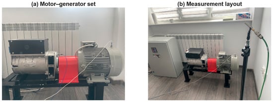
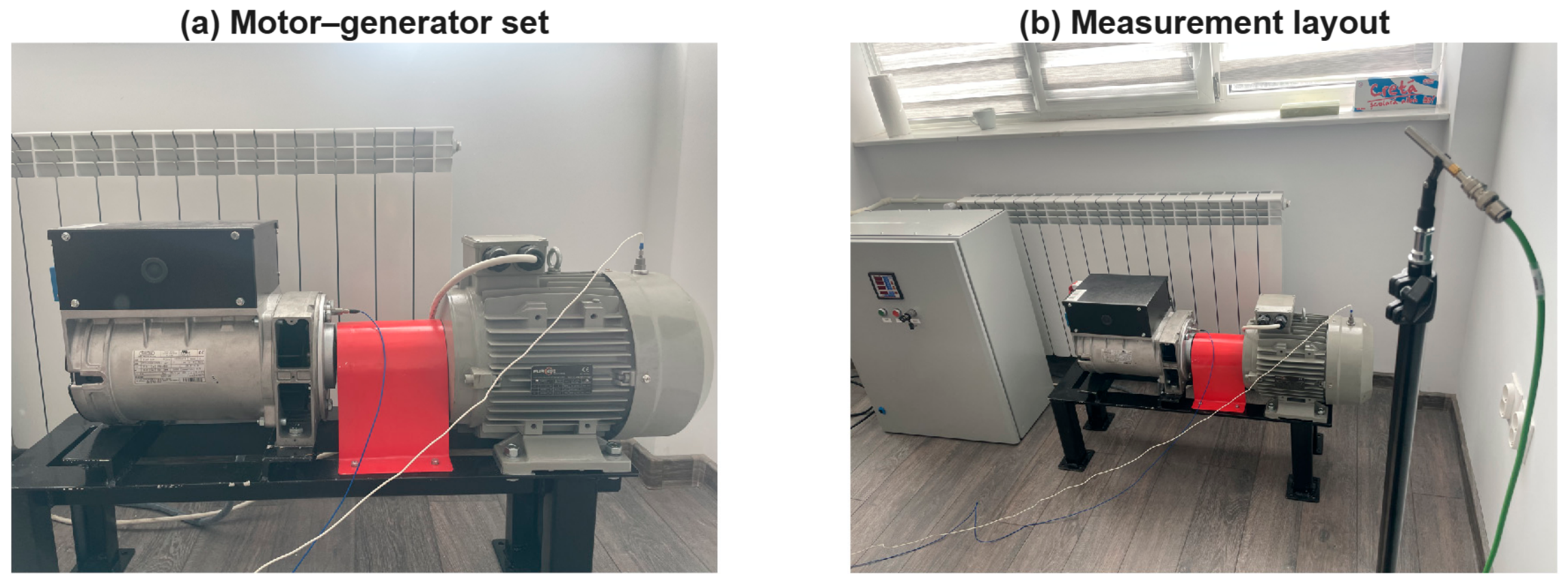
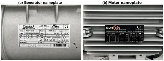
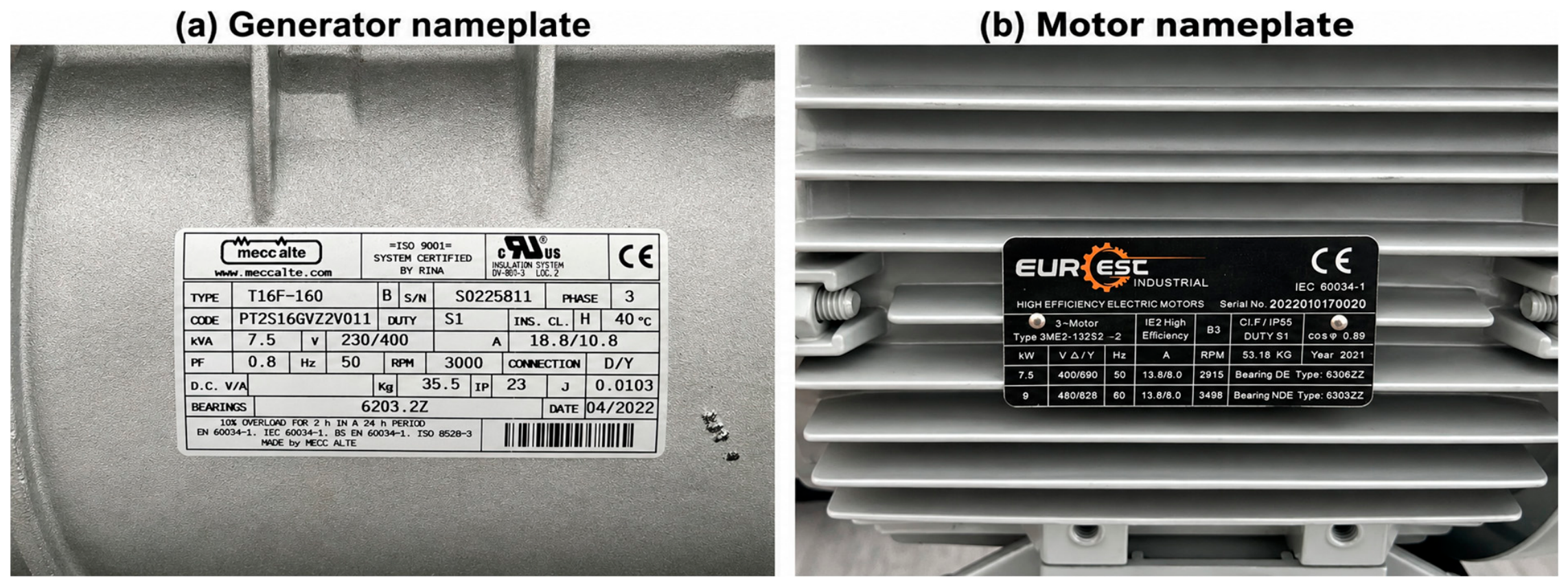
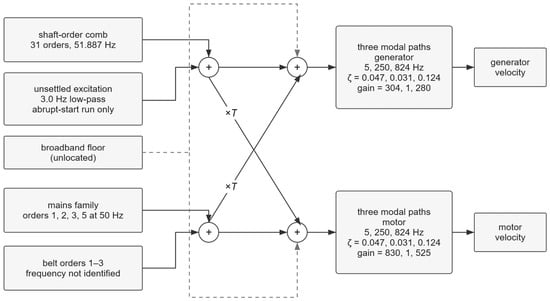
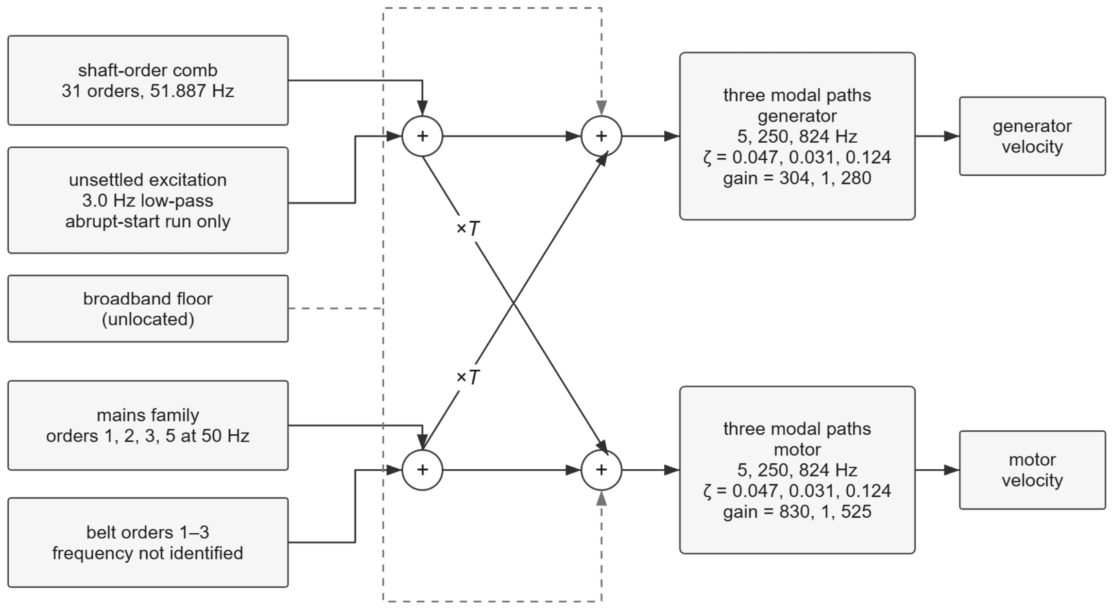
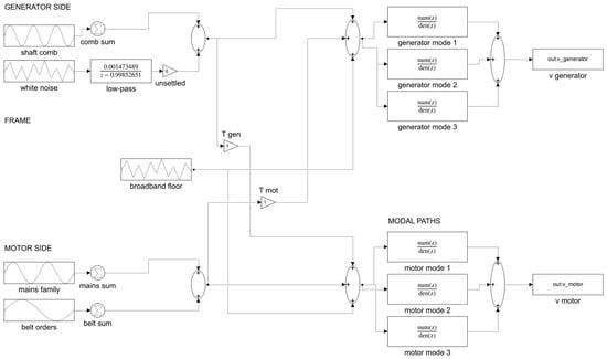
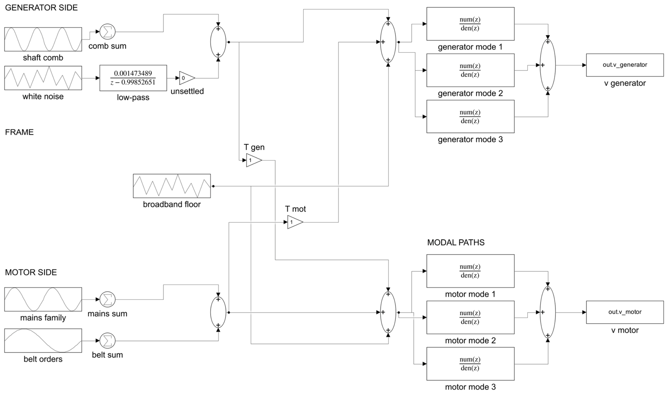
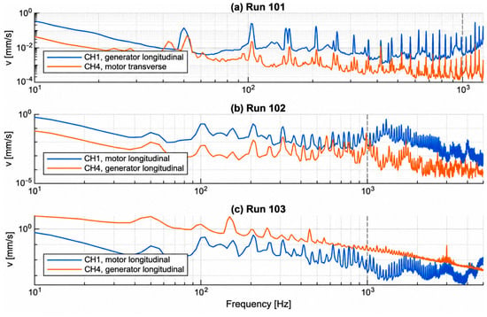
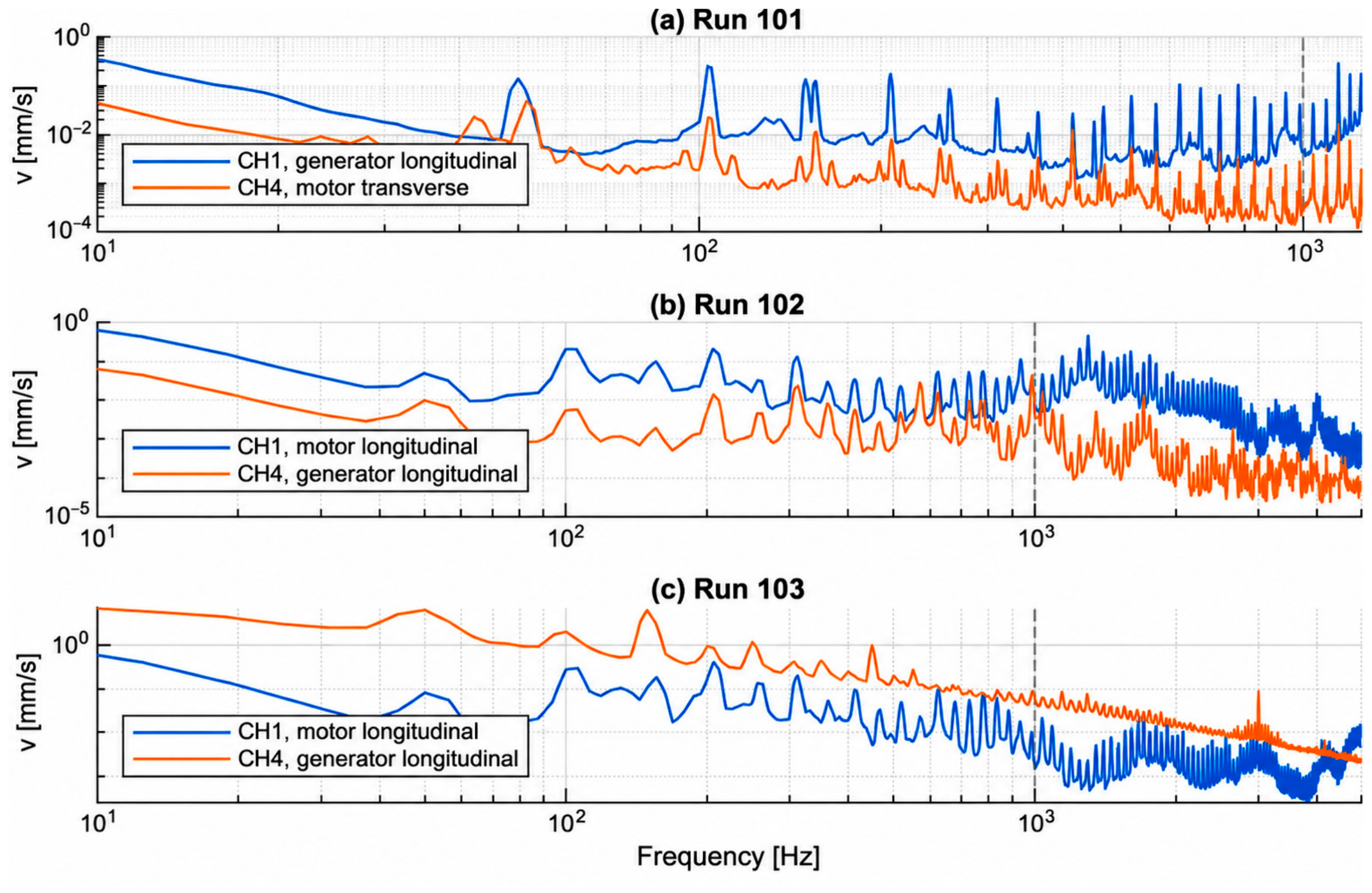
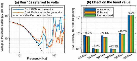
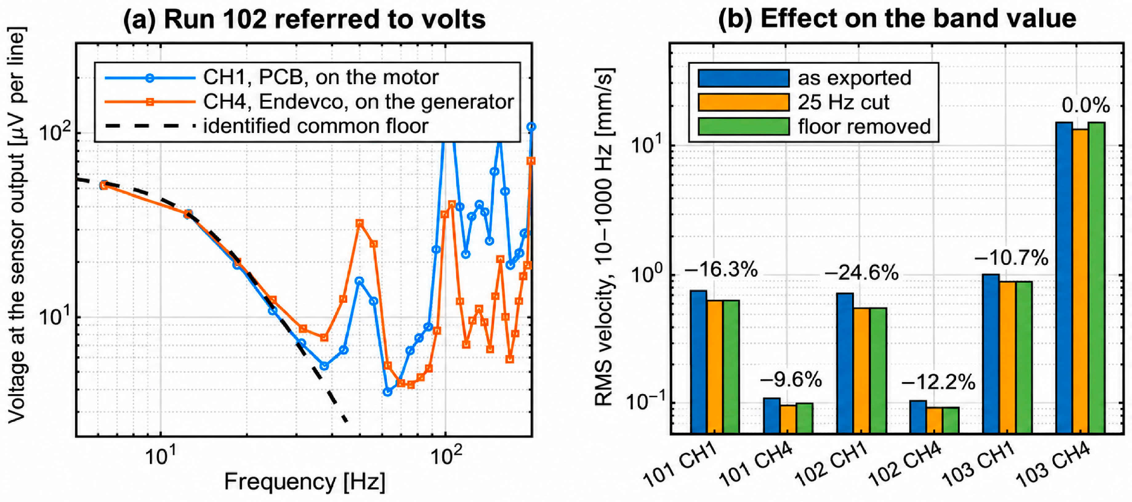
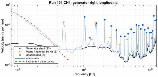
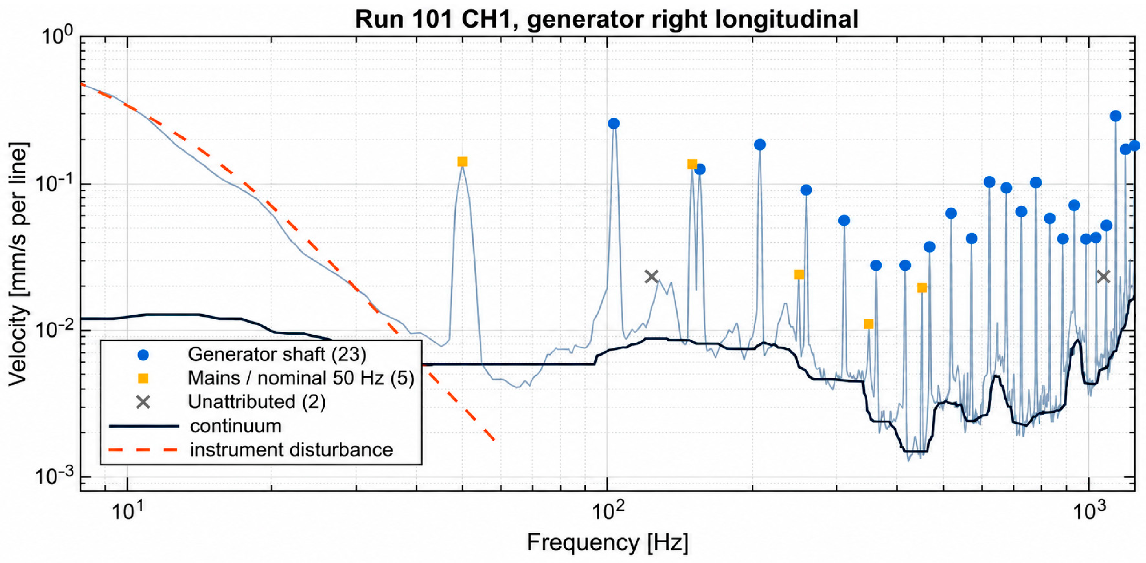
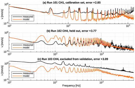
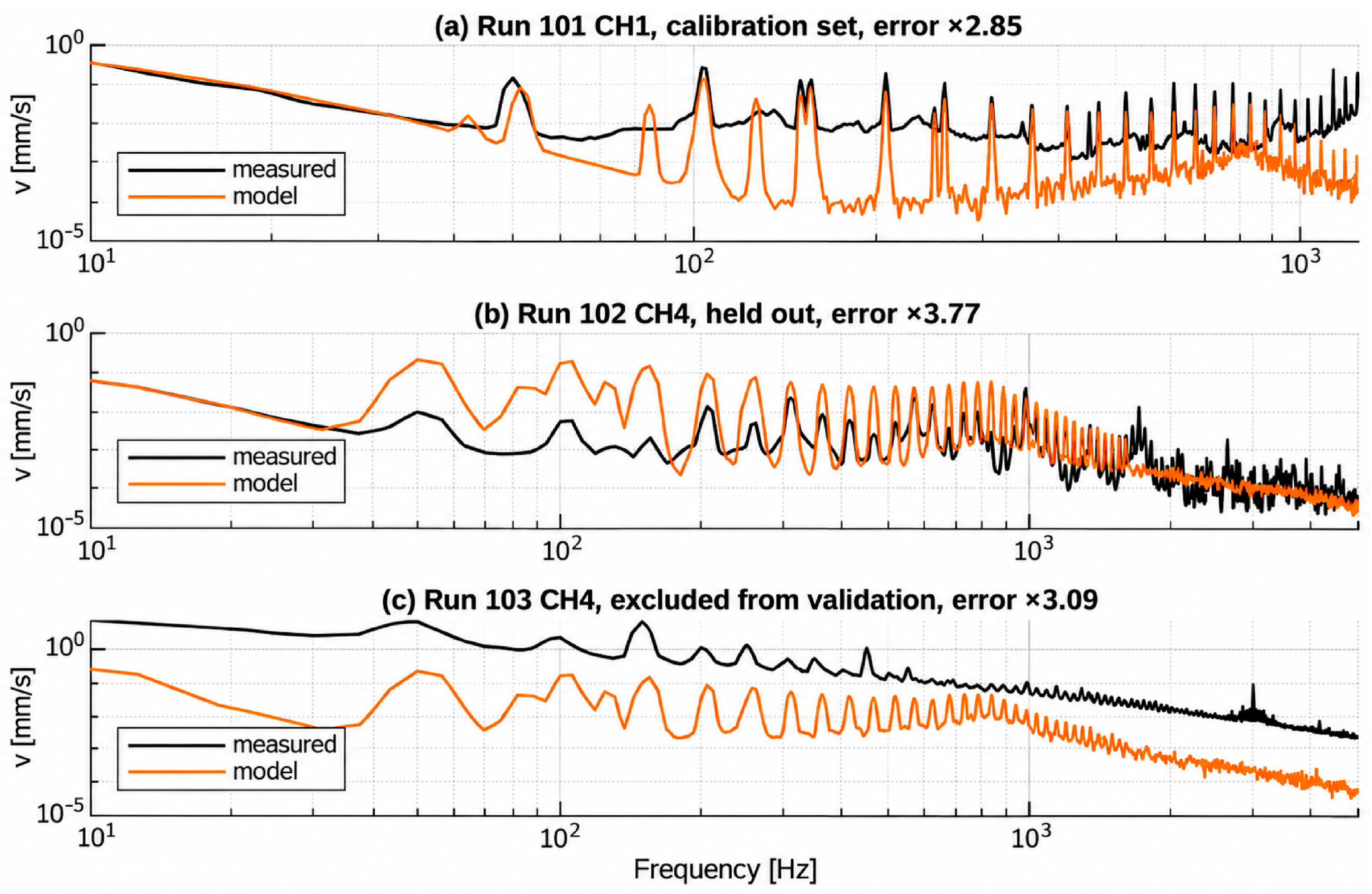
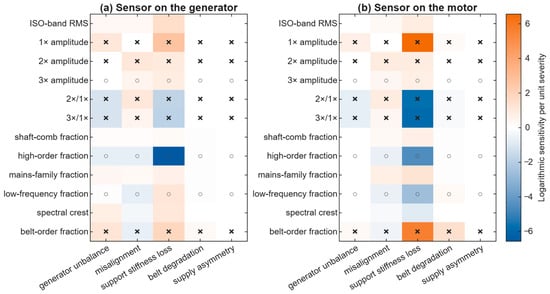
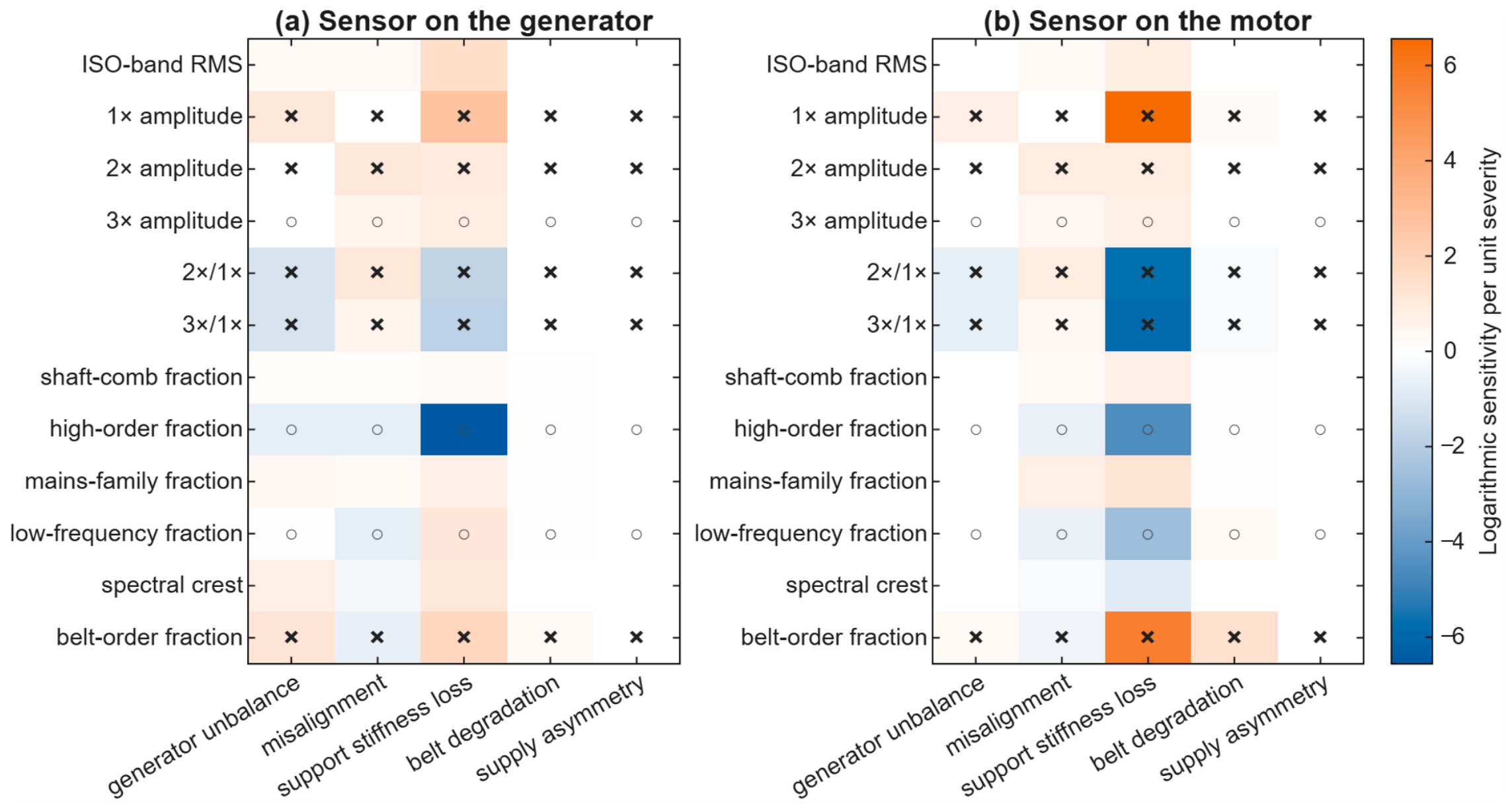
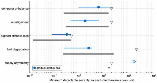
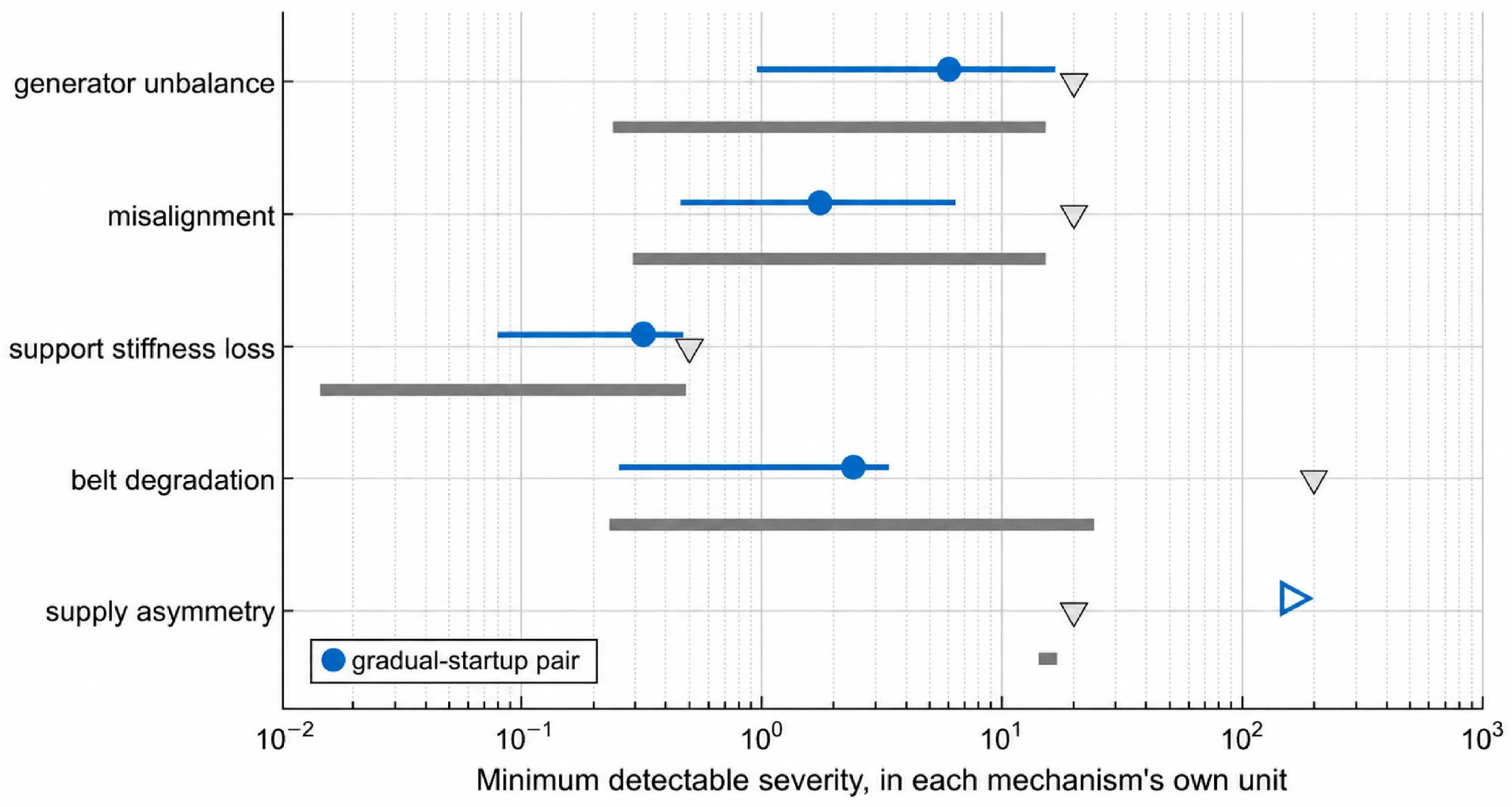
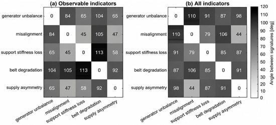
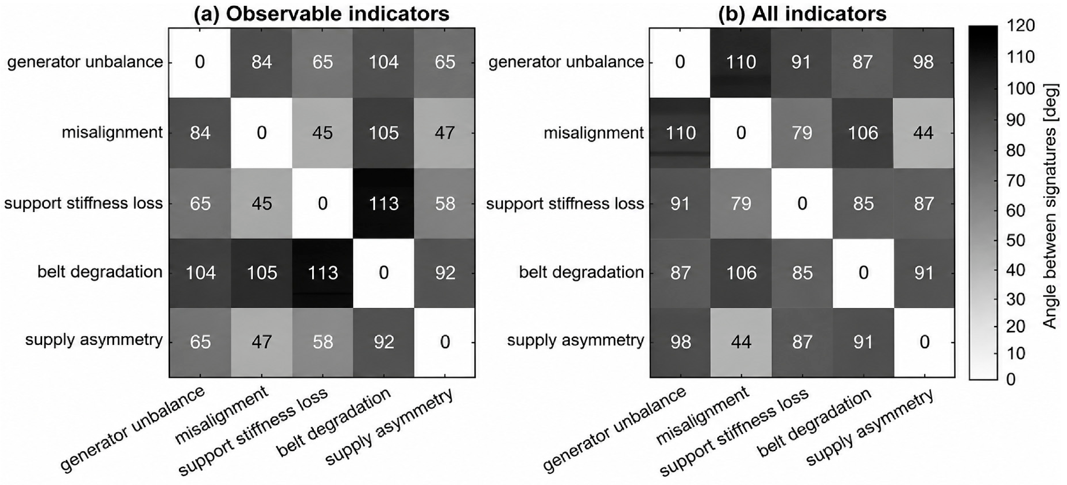
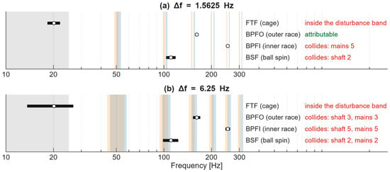
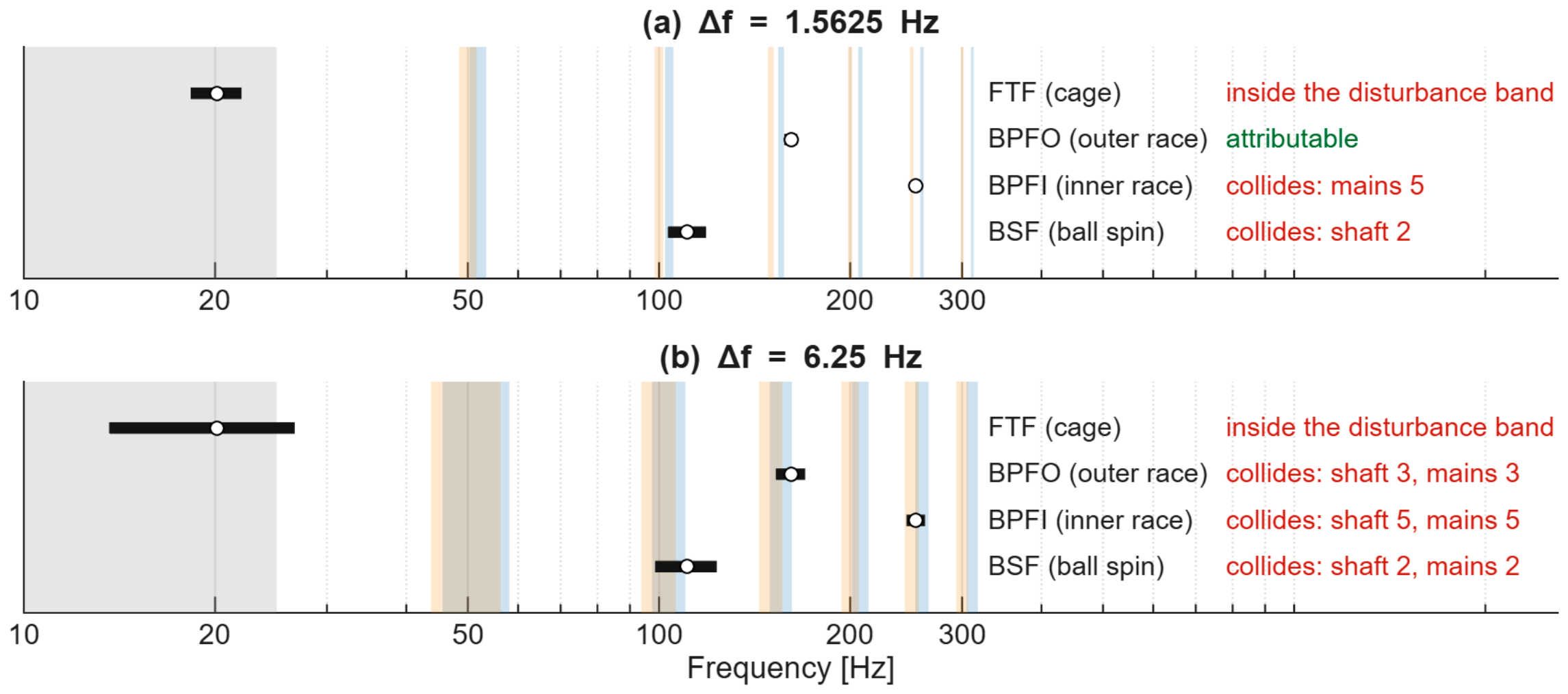

Disclaimer/Publisher’s Note: The statements, opinions and data contained in all publications are solely those of the individual author(s) and contributor(s) and not of MDPI and/or the editor(s). MDPI and/or the editor(s) disclaim responsibility for any injury to people or property resulting from any ideas, methods, instructions or products referred to in the content. |
© 2026 by the authors. Licensee MDPI, Basel, Switzerland. This article is an open access article distributed under the terms and conditions of the Creative Commons Attribution (CC BY) license.