An Exponential Sliding-Mode Observer with a Continuous Boundary Layer for Position-Sensorless IPMSM Drives

Abstract

This study presents an exponential sliding-mode observer with a continuous boundary layer for position-sensorless interior permanent magnet synchronous motor drives. The observer combines linear and fractional-power error feedback with a smooth switching function. The exponential reaching law provides finite-time convergence, while the continuous observer analysis establishes ultimate boundedness and finite-time entry into the prescribed boundary layer under bounded forcing. Compared with a super-twisting sliding-mode observer, the proposed method achieves smaller speed-estimation error, lower current distortion, and reduced calculated torque fluctuations in the reported tests. The speed-reversal experiments further demonstrate accurate rotor-position tracking at commanded speeds of ±500 and ±1000 r/min. Component-ablation results confirm the combined contribution of the linear reaching term and continuous smoothing mechanism to the estimation performance.

1. Introduction

Electric vehicles, industrial robots, and other demanding drive systems increasingly employ permanent magnet synchronous motors (PMSMs) because they offer a favorable power-to-volume ratio and responsive dynamics. High-performance control depends on precise knowledge of the rotor position and rotational speed. Although mechanical sensors provide these quantities directly, they increase hardware cost and occupied space, and their reliability may deteriorate in severe operating environments [1,2,3]. Eliminating these devices while maintaining control performance has therefore made sensorless estimation an important research topic in electrical drives.

Sensorless methods based on high-frequency signal injection exploit motor saliency at low speed [4,5,6,7], whereas fundamental-model methods use voltage, current, and flux or back-EMF information [8,9,10]. Sliding-mode observation is one of the established approaches in this latter group [11,12]. Related developments include extended-state observation with position extraction [13] and model-reference adaptive estimation [14]. Extended Kalman filtering (EKF) has also been investigated with a neural magnetic model for synchronous reluctance drives [15] and with adaptive noise-covariance estimation for PMSM drives [16]. These studies address model representation, implementation, and covariance tuning. Adaptive sliding-mode and back-EMF observation provide further alternatives [17,18]. Discontinuous injection can introduce chattering; filtering the recovered signal can also alter its amplitude and phase. These effects motivate examination of the estimation error and the complete signal-recovery path.

Recent approaches include a high-order terminal sliding-mode observer [19], a barrier-function adaptive super-twisting observer combined with fixed-time control [20], and a state-dependent reaching-law design for PMSM speed regulation with observer-based speed estimation [21]. Fuzzy sliding-mode designs [22] provide another alternative. Building on exponential reaching and continuous saturation concepts, the present study develops an observer structure that combines linear and fractional-power current-error feedback with a saturated piecewise-quadratic boundary layer. The linear and fractional-power terms shape the error-dependent restoring action, while the piecewise-quadratic boundary layer provides a continuous transition near zero. The comparison focuses on estimation accuracy and transient response.

The distinctions from [19,20,21] concern the injection structure and its analysis. Reference [19] uses a high-order terminal observer, whereas Equations(11) and (12) apply the linear and fractional-power terms directly to the current-estimation error, with a continuous piecewise-quadratic transition near zero. Reference [20] adapts super-twisting gains through a barrier function; the present injection instead uses prescribed gains and an explicit boundary-layer width, without an adaptive gain law. Reference [21] develops a state-dependent reaching law for speed regulation and a sliding-mode observer incorporating a back-EMF observer; the present formulation focuses on current-error injection and residual-voltage recovery in an IPMSM model that retains saliency. Its specific analytical contribution is to relate the proposed injection structure to forced-error bounds, sufficient conditions for boundary-layer entry, and residual-voltage recovery. The continuous boundary layer removes the injection discontinuity near the origin, while the linear and fractional-power terms provide complementary error-restoring actions. These characteristics are further evaluated experimentally in Section 4.

The proposed observer retains the label FTESMO to identify the scheme and the corresponding records. In this label, finite time refers to the ideal reaching law analyzed in Section 3.1. The continuous implementation in Section 3.2 is treated as nonlinear error feedback with a boundary layer. The comparison addresses rated-load steady operation, speed reversal, and torque-reference tracking. Section 4.5 compares the complete observer with variants that remove the linear reaching term or replace the smooth switching function by signum injection. This comparison examines the contribution of each component at the adopted parameter setting.

2. Permanent Magnet Synchronous Motor and Sliding-Mode Observer

2.1. Saliency-Aware IPMSM Model

The test motor is an interior permanent magnet synchronous motor (IPMSM) with unequal d- and q-axis inductances. With constant inductances and magnetic saturation, eddy-current loss, and hysteresis neglected, its stationary-frame voltage can be decomposed into a q-axis-inductance current term and a residual-voltage vector. This decomposition retains saliency through the active flux and gives the voltage equation below.

u_αβ = R_si_αβ + L_qi_αβ + e_a

(1)

Here, the stationary-frame voltage and current symbols denote two-component column vectors on the α and β axes. The q-axis inductance is used as the constant inductance in Equation (1). Define the inductance difference as the d-axis inductance minus the q-axis inductance. The active flux is the permanent-magnet flux linkage plus this inductance difference multiplied by the d-axis current. The direct-axis unit vector has cosine and sine components, whereas the quadrature-axis unit vector has negative-sine and cosine components, both evaluated at the electrical rotor angle. Differentiating the active-flux vector gives the residual voltage in Equation (2).

$$e_a={\dot{\psi }}_{a}d({\theta }_e)+{\omega }_e{\psi }_{a}q({\theta }_e),\hspace{1em}\hspace{1em}{\dot{\psi }}_a=\Delta L{\dot{i}}_d$$

(2)

The two contributions in Equation (2) arise from variation in the active-flux magnitude and rotation of its direction, respectively. Consequently, the residual voltage is not generally identical to the permanent-magnet-only back-EMF. The electrical angular velocity is the time derivative of the electrical rotor angle. Rearranging Equation (1) gives the current dynamics in Equation (3). The use of a constant q-axis inductance in this decomposition does not impose equal d- and q-axis inductances: the saliency contribution remains in the active flux and its derivative. The observer design selects L = L_q = 9.75 mH as the nominal inductance in Equation (5), while L_d = 4.25 mH is retained through the inductance difference in the active flux and torque expression. Thus, the use of a single constant inductance in the current dynamics does not discard the motor saliency.

The residual voltage in Equation (2) contains a component parallel to the direct-axis unit vector whenever the active-flux magnitude varies. Its direction is then not exactly in quadrature with the rotor flux. Thus, the constant q-axis-inductance decomposition is compatible with saliency, but the simple arctangent extraction in Section 3.3 additionally requires the active-flux magnitude to vary slowly relative to its rotational contribution. The model decomposition and the position-extraction approximation play different roles: the former retains the IPMSM saliency, whereas the latter is used for rotor-position extraction under the operating conditions considered in this study.

$${\stackrel{.}{i}}_{\mathit{\alpha \beta }}=-{\displaystyle \frac{R_s}{L_q}}{i}_{\mathit{\alpha \beta }}+{\displaystyle \frac{u_{\mathit{\alpha \beta }}-e_a}{L_q}}$$

(3)

For the IPMSM, electromagnetic torque is calculated from the electrical quantities using the following expression, which includes both the permanent-magnet and reluctance torque components.

$$T_e={\displaystyle \frac{3}{2}}{p}_n\left[{\psi }_f{i}_q+(L_d-L_q)i_d{i}_q\right]$$

(4)

In this expression, the pole-pair number and permanent-magnet flux linkage are motor parameters, and the d- and q-axis currents are the current components in the rotor reference frame. The first term gives the permanent-magnet torque, while the second gives the reluctance torque arising from the difference between the d- and q-axis inductances. Both contributions are retained for the interior permanent magnet motor considered here.

2.2. Traditional and Second-Order Sliding-Mode Observers

For each stationary axis, the observer uses the applied voltage and an injection signal to reconstruct current. The observation error is estimated current minus measured current. In Equation (5), L denotes the nominal observer inductance, selected as the q-axis inductance for consistency with Equations (1)–(3), and the scalar back-EMF symbol denotes the corresponding component of the residual voltage in Equation (2). Subtracting the plant dynamics from the observer gives the error equation below. The additive mismatch term collects deviations from the nominal current dynamics and has units of current per unit time.

$$\begin{array}{l}{\dot{\widehat{i}}}_x=-{\displaystyle \frac{R_s}{L}}{\widehat{i}}_x+{\displaystyle \frac{u_x-v_x}{L}},\hspace{1em}\hspace{1em}{s}_x={\widehat{i}}_x-i_x,\hspace{1em}\hspace{1em}x\in \{\alpha ,\beta \}\\ {\dot{s}}_x=-{\displaystyle \frac{R_s}{L}}{s}_x+{\displaystyle \frac{e_x-v_x}{L}}+{\delta }_x\end{array}$$

(5)

A conventional signum injection uses the sign of the current observation error. Its reachability requires an injection magnitude sufficient to dominate the relevant bounded forcing. Discrete switching can introduce chattering, and an additional low-pass filter, when used, changes the amplitude and phase of the recovered signal.

A super-twisting observer introduces an auxiliary injection state and a signum-driven update. Equation (6) gives the comparison structure. Its current-error symbol denotes the same estimated-minus-measured difference as in Equation (5). The gains in this STASMO expression are specific to the comparison observer and are distinct from the gains subsequently used for FTESMO.

$$\left\{\begin{array}{l}v=k_1|\tilde{i}{|}^{1/2}\mathrm{sgn}(\tilde{i})+\eta \hfill \\ \dot{\eta }=k_2\cdot \mathrm{sgn}(\tilde{i})\hfill \end{array}\right.$$

(6)

The super-twisting algorithm provides a continuous injection under its associated regularity and gain conditions. Its experimental performance is compared with the proposed observer under identical control and operating settings in Section 4.

3. Exponential Sliding-Mode Observer with a Continuous Boundary Layer

3.1. Ideal Unforced Exponential Reaching Law

The ideal reaching law combines a linear term with a fractional-power term. Its unforced scalar dynamics are analyzed first, separately from the forced observer error dynamics and from the subsequent boundary-layer implementation.

3.1.1. Reaching-Law Dynamics Analysis

Defining the sliding-mode variable as s, the designed reaching law dynamic equation is

$$\dot{s}=-k_{1}s-k_2|s{|}^{\gamma }\mathrm{sgn}(s)$$

(7)

The gains k₁ and k₂ are positive and the exponent γ lies strictly between zero and one. Their dimensions must be consistent with the units of the sliding variable. The crossover between the two terms depends on both gains and the chosen error units.

For sufficiently large error magnitude, the linear term dominates the fractional-power term and gives exponential decay in the ideal reaching dynamics. There is no universal crossover at an error magnitude of one; the crossover is determined by equality of the two term magnitudes.

Near the origin, the fractional-power term dominates the linear term in the ideal unforced law. Its magnitude nevertheless tends to zero. Its unbounded slope permits finite-time convergence of that ideal law, but does not supply a nonzero injection at zero error capable of balancing a nonzero back-EMF.

3.1.2. Convergence of the Ideal Unforced Reaching Law

For the ideal scalar dynamics in Equation (7), a quadratic Lyapunov candidate gives the derivative below. This calculation does not yet include the back-EMF forcing, parameter mismatch, saliency, or the continuous boundary layer of the implemented observer.

$$\dot{V}=s\dot{s}=-k_1{s}^2-k_2{|s|}^{\gamma +1}=-2k_{1}V-2^{{\displaystyle \frac{\gamma +1}{2}}}{k}_2{V}^{{\displaystyle \frac{\gamma +1}{2}}}\le 0$$

(8)

The derivative is negative for nonzero error in the ideal unforced system. Separating variables gives its reaching time from a specified initial error to the origin.

$${\displaystyle {\int }_0^{T_{\mathrm{conv}}}d}t={\displaystyle {\int }_{s(0)}^0\frac{\mathit{ds}}{-k_{1}s-k_2|s{|}^{\gamma }\mathrm{sgn}(s)}}$$

(9)

Solving the above integral, the analytical expression for the convergence time is obtained

$$T_{\mathrm{conv}}={\displaystyle \frac{1}{k_1(1-\gamma )}}\ln \left({\displaystyle \frac{k_1|s(0){|}^{1-\gamma }+k_2}{k_2}}\right)$$

(10)

Equation (10) gives the finite reaching time of the ideal unforced law as an explicit function of the initial error, observer gains, and exponent. For the continuous observer subject to residual-voltage forcing and model mismatch, the convergence analysis is extended to practical boundary-layer convergence. The following derivation establishes ultimate boundedness and, under condition Equation (21), finite-time entry into the prescribed boundary layer.

3.2. Observer Construction Based on Continuous Smooth Switching Function

The proposed continuous injection replaces the signum function with a continuous boundary-layer function. Accordingly, the near-origin dynamics are described by the forced boundary-layer model developed below. The injection is defined below.

$$v_x=L_s(k_1{\tilde{i}}_x+k_2|{\tilde{i}}_x{|}^{\gamma }Z({\tilde{i}}_x,\sigma ))$$

(11)

The current-error notation in Equations (11) and (12) denotes the same axis error introduced in Equation (5), and the inductance factor denotes the same nominal inductance. It converts the current-rate feedback into a voltage injection. The saturated piecewise-quadratic switching function is given by Equation (12).

$$Z({\tilde{i}}_x,\sigma )=\left\{\begin{array}{ll}\mathrm{sgn}({\tilde{i}}_x),\hfill & \left|{\tilde{i}}_x\right|>\sigma \hfill \\ {\displaystyle \frac{2{\tilde{i}}_x}{\sigma }}-\mathrm{sgn}({\tilde{i}}_x){\left({\displaystyle \frac{{\tilde{i}}_x}{\sigma }}\right)}^2,\hfill & \left|{\tilde{i}}_x\right|\le \sigma \hfill \end{array}\right.$$

(12)

The positive boundary-layer width is expressed in current-error units. Outside this layer, the switching function is the sign of the error; inside it, the injection varies continuously. Near zero, the nonlinear part vanishes faster than the current error, leaving a finite linear feedback gain. The resulting forced-error dynamics must therefore be analyzed separately from the ideal reaching law.

Substitution of the injection Equation (11) into the error dynamics Equation (5), using the common current-error and inductance notation, gives the forced scalar system Equation (13).

$${\dot{s}}_x=-a{s}_x-k_2|s_x{|}^{\gamma }Z(s_x,\sigma )+d_x(t)$$

(13)

The linear decay coefficient and the total forcing are defined in Equation (14). For each stationary axis, assume that the total forcing is measurable and uniformly bounded over the operating domain considered. This is an explicit hypothesis of the following continuous-time analysis. The bound includes the residual voltage itself, divided by the nominal inductance, together with the additive model-mismatch contribution; it is not merely a parameter-uncertainty bound. A sufficient conservative bound is obtained by adding a bound on the absolute residual voltage divided by the nominal inductance to a bound on the absolute mismatch term. For the IPMSM decomposition in Equation (2), bounding the residual voltage requires bounds on electrical speed, active-flux magnitude, and the rate of change in that magnitude. These bounds must cover the specified transients as well as steady operation. Accordingly, the forcing bound is formulated to cover both the specified transients and steady-state operation over the considered operating domain.

$$a={\displaystyle \frac{R_s}{L}}+k_1>0,\hspace{1em}\hspace{1em}{d}_x={\displaystyle \frac{e_x}{L}}+{\delta }_x,\hspace{1em}\hspace{1em}|d_x(t)|\le D_x$$

(14)

To assess boundedness for either stationary axis, select the nonnegative quadratic Lyapunov function in Equation (15).

$$V_x={\displaystyle \frac{1}{2}}{s}_x^2$$

(15)

Differentiating along Equation (13), using the common sign of the switching function and the error, and applying the forcing bound in Equation (14) yields Equation (16). This expression explicitly reveals the competition between the restoring terms and the bounded external forcing and forms the basis for the ultimate-bound analysis.

$${\dot{V}}_x\le -a{s}_x^2-k_2\left|s_x{|}^{\gamma +1}\right|Z(s_x,\sigma )|+D_x|s_x|$$

(16)

For a nonnegative error magnitude r, define the magnitude of the switching function by Equation (17). This expression is continuous, nonnegative, and nondecreasing.

$$z(r)=\left\{\begin{array}{ll}{\displaystyle \frac{2r}{\sigma }}-{\left({\displaystyle \frac{r}{\sigma }}\right)}^2,\hfill & 0\le r\le \sigma ,\hfill \\ 1,\hfill & r>\sigma \hfill \end{array}\right.$$

(17)

Collect the linear and nonlinear restoring terms in the scalar function Equation (18). This function is continuous, strictly increasing, zero at the origin, and unbounded as r increases.

g(r) = ar + k₂r^γz(r)

(18)

Away from zero, the upper right derivative of the error magnitude is bounded by the forcing bound minus this restoring function. The same upper-derivative inequality holds at zero. Hence there is a unique nonnegative balance radius, and the scalar comparison argument gives Equation (19): for every radius larger than that balance radius, the error magnitude has a strictly inward derivative until it enters that radius.

$$g(r_x^{*})=D_x,\hspace{1em}\hspace{1em}\underset{t\to \infty }{\lim \sup }|s_x(t)|\le r_x^{*}$$

(19)

Since the switching-function magnitude equals one at the boundary, the sufficient condition Equation (20) makes the closed boundary layer forward invariant. Under this condition, the balance radius in Equation (19) does not exceed the boundary-layer width. For a prescribed positive layer width and an exponent strictly between zero and one, positive gains can be selected so that the restoring magnitude at the boundary exceeds the forcing bound. If the same gains are used on both stationary axes, this comparison must use the larger of the two axis-specific forcing bounds. Thus, gain selection explicitly accounts for the residual-voltage forcing, rather than assuming that the vanishing nonlinear injection cancels it at zero error.

aσ + k₂σ^γ ≥ D_x

(20)

Finite-time entry from outside the layer requires the strict positive margin defined in Equation (21). Here the subscripted margin symbol is local to this bound and is distinct from the auxiliary STASMO state in Equation (6).

η_x = aσ + k₂σ^γ − D_x > 0

(21)

Outside the layer, monotonicity of the restoring function makes the inward rate at least this margin. Integrating that rate gives the entry-time bound Equation (22); an initial error already inside the layer has zero entry time.

$$T_{\sigma ,x}\le {\displaystyle \frac{\max \left\{\right|s_x(0)|-\sigma ,0\}}{{\eta }_x}}$$

(22)

Equations (19)–(22) establish ultimate boundedness of the forced observer and provide a sufficient condition for finite-time entry into the prescribed boundary layer. Condition Equation (20) guarantees forward invariance of the boundary layer, whereas the strict positive margin in Equation (21) determines the finite entry-time bound in Equation (22). The analysis explicitly incorporates residual-voltage forcing and bounded model mismatch, thereby extending the ideal reaching-law analysis to the practical observer error dynamics.

The resistance contribution is retained in the linear decay coefficient in Equation (14); it has not been removed from the forced-error dynamics. The non-strict boundary inequality Equation (20) establishes forward invariance, whereas the strict inequality Equation (21) supplies the positive margin needed for the finite entry-time bound Equation (22). The ultimate radius in Equation (19) is a limiting bound: finite-time entry is guaranteed into any strictly larger radius, not necessarily into the balance radius itself. These conclusions apply separately to the two stationary-axis errors under their forcing bounds.

The injection output is used as the recovered residual-voltage estimate in Equation (23), and its relationship with the true residual voltage is characterized by the bias relation derived in Equation (24).

$${\widehat{e}}_x:=v_x$$

(23)

Rearranging the error Equation Equation (5) and applying the definition Equation (23) gives the exact nominal-coordinate bias relation Equation (24), with the mismatch term retained.

$${\widehat{e}}_x-e_x=-R_s{s}_x-L{\dot{s}}_x+L{\delta }_x$$

(24)

The triangle inequality then gives the magnitude bound in Equation (25). When the nominal model matches the plant, the mismatch contribution vanishes, while the current-error and error-derivative contributions can remain.

$$|{\widehat{e}}_x-e_x|\le R_s\left|s_x\right|+L\left|{\dot{s}}_x\right|+L\left|{\delta }_x\right|$$

(25)

Equation (25) characterizes the residual-voltage estimation error in terms of the current-estimation error, its derivative, and model mismatch. This relation provides a direct theoretical link between observer error dynamics and residual-voltage recovery accuracy. The position and speed extraction scheme in Section 3.3, together with the waveform comparison in Section 4.4, is used to evaluate the resulting amplitude and phase characteristics.

The influence of operating speed and boundary-layer width is interpreted through the forced observer dynamics. With the active-flux magnitude held fixed, the rotational contribution to the residual voltage increases with electrical speed, while active-flux variation introduces an additional transient component. At fixed error magnitude and observer gains, the boundary-layer width modifies the magnitude of the smoothed nonlinear injection and consequently affects the conservative error bound. Together with the bias relation in Equation (24), these results establish the theoretical relationship among operating condition, boundary-layer width, current-estimation error, and residual-voltage recovery.

The boundary-layer width σ is positive and is expressed in the same units as the current-estimation error. Its selection is considered jointly with the observer gains and the forcing bound through Equations (20) and (21). A smaller σ produces a narrower transition region and stronger nonlinear correction near the boundary, whereas a larger σ enlarges the smooth transition region. Therefore, σ provides a direct tuning mechanism for balancing estimation-error suppression and injection smoothness. The adopted value is selected according to this trade-off.

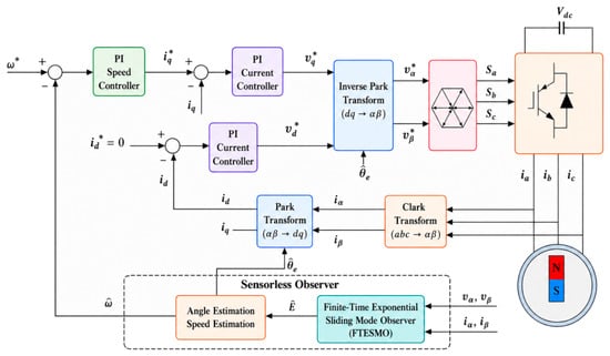
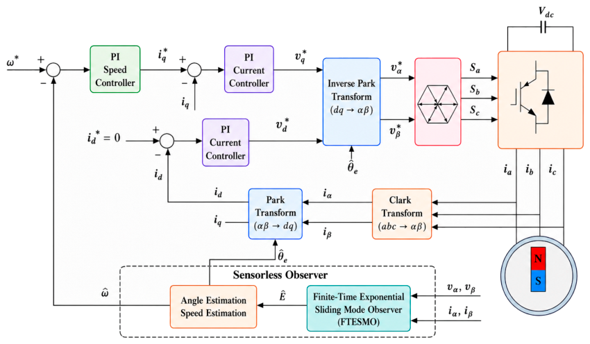
Figure 1 presents the control structure labeled FTESMO.

Figure 1. Overall block diagram of the position-sensorless PMSM control system based on FTESMO.

3.3. Rotor Position and Speed Extraction

In the proposed extraction scheme, the rotor electrical position is obtained using the arctangent method from the two stationary-frame components of the recovered residual-voltage vector. The two-argument arctangent is used to retain quadrant information and avoid explicit division by a component that may approach zero. Under the axis convention adopted in Section 2.1, the negative alpha-axis component and the beta-axis component form the two arctangent inputs. This gives an approximate rotor-position estimate when variation in the active-flux magnitude is negligible relative to its rotational contribution.

$${\widehat{\theta }}_{e,w}(t)={\mathrm{wrap}}_{2\pi }\left[\mathrm{atan}2\left(-{\widehat{e}}_{\alpha }(t),{\widehat{e}}_{\beta }(t)\right)-{\delta }_{\mathrm{dir}}(t)\right]$$

(26)

The mechanical speed is obtained by differentiating the unwrapped, direction-consistent arctangent phase and converting electrical angular velocity to r/min. The following compact relation summarizes the steps detailed in Equations (28)–(30).

$${\widehat{n}}_m(t)={\displaystyle \frac{60}{2\pi p_n}}{\displaystyle \frac{\mathrm{d}}{\mathrm{d}t}}\mathrm{unwrap}\left[\mathrm{atan}2\left(-{\widehat{e}}_{\alpha }(t),{\widehat{e}}_{\beta }(t)\right)-{\delta }_{\mathrm{dir}}(t)\right]$$

(27)

The direction-dependent phase correction in this expression is zero for positive rotation and pi radians for negative rotation, assuming positive active flux. It accounts for reversal of the residual-voltage vector when the rotation direction changes. The extraction relationship assumes that a consistent rotation-direction branch is available; the arctangent ratio alone cannot resolve this ambiguity. The extraction formula requires a sufficiently large residual-voltage magnitude for reliable phase calculation.

Before speed calculation, the estimated electrical angle is unwrapped to obtain a continuous phase sequence. Unwrapping removes artificial jumps at the angle-wrapping boundary while retaining the physical change in rotor position. It does not by itself resolve a direction-dependent pi ambiguity. Phase unwrapping requires successive sampled phase increments to be resolvable without an unknown full-cycle ambiguity.

$${\widehat{\theta }}_{e,u}(t)=\mathrm{unwrap}\left({\widehat{\theta }}_{e,w}(t)\right)$$

(28)

The estimated electrical angular velocity is obtained from the time derivative of the continuous electrical angle. For a sampled realization of this scheme, this derivative is approximated by the difference between consecutive angle samples divided by the sampling period. The electrical angular velocity is then divided by the pole-pair number to obtain mechanical angular velocity and converted to revolutions per minute.

$${\widehat{n}}_m(t)={\displaystyle \frac{60}{2\pi p_n}}{\displaystyle \frac{\mathrm{d}{\widehat{\theta }}_{e,u}(t)}{\mathrm{d}t}}$$

(29)

$${\widehat{n}}_m[k]={\displaystyle \frac{60}{2\pi p_n{T}_s}}\left({\widehat{\theta }}_{e,u}[k]-{\widehat{\theta }}_{e,u}[k-1]\right)$$

(30)

Here, the sampling period is expressed in seconds, the continuous electrical angle in radians, and the pole-pair number is the same motor parameter used in the electromagnetic-torque expression. The resulting speed retains its sign, distinguishing forward and reverse rotation. Angle differentiation can amplify phase noise; therefore, position accuracy and speed accuracy are evaluated separately. Equations (26)–(30) specify the proposed scheme of arctangent extraction followed by angle differentiation and speed conversion. Equations (26)–(30) define the complete rotor-position and speed extraction procedure, including arctangent phase extraction, phase unwrapping, discrete differentiation, pole-pair conversion, and mechanical-speed calculation.

4. Experimental Results and Discussion

The experimental evaluation compares FTESMO with STASMO under identical drive-control settings. The current-loop and speed-loop controllers, their gains, sampling and switching settings, current and voltage limits, motor parameters, and reference commands are kept unchanged, so that the observed differences primarily reflect the observer configuration. The experiments include rated-load steady-state operation, speed reversal among +1000, +500, −500, and −1000 r/min, and torque-reference tracking. These operating conditions provide evaluation of both steady-state estimation accuracy and transient performance during forward and reverse operation.

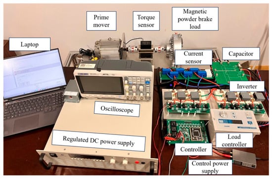
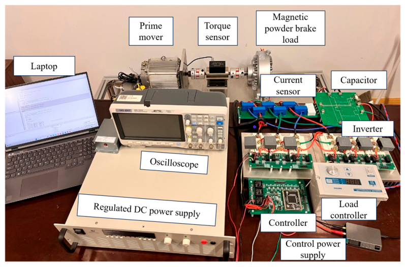
Figure 2 shows the reported validation platform. The comparison uses the available steady-state, speed-reversal, and torque-reference records. The proposed angle and speed extraction scheme is described in Section 3.3, and the electromagnetic torque is calculated from electrical quantities using the expression in Section 2.1. The DC-link voltage is 100 V, and the sampling frequency is 10 kHz, corresponding to a sampling period of 100 microseconds. A resolver provides the reference rotor-position information used to obtain the actual angle and speed traces for comparison with the observer estimates.The motor parameters used in this experiment are listed in Table 1.

Figure 2. Experimental platform used for the PMSM sensorless control verification.

Table 1. Motor parameters.

Parameter	Value
Rated torque Te/(N·m)	8
Permanent magnet flux linkage ψf/Wb	0.1325
Number of pole pairs pn	4
Stator resistance Rs/Ω	0.4156
d-axis stator inductance Ld/mH	4.25
q-axis stator inductance Lq/mH	9.75
Moment of inertia J/(kg·m2)	0.0047

Table 1. Motor parameters.

Parameter	Value
Rated torque Te/(N·m)	8
Permanent magnet flux linkage ψf/Wb	0.1325
Number of pole pairs pn	4
Stator resistance Rs/Ω	0.4156
d-axis stator inductance Ld/mH	4.25
q-axis stator inductance Lq/mH	9.75
Moment of inertia J/(kg·m2)	0.0047

4.1. Rated-Load Steady-State Experiment

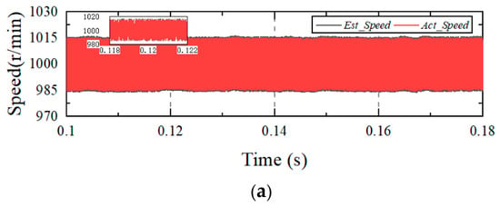
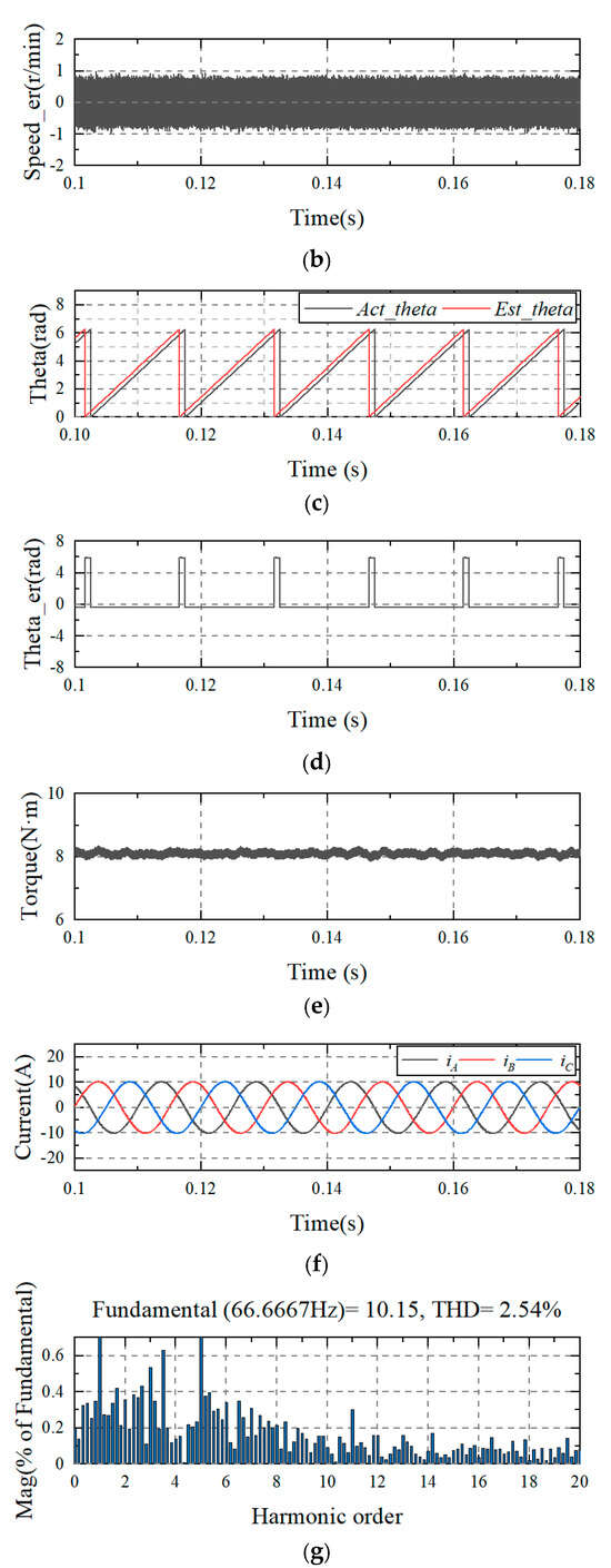
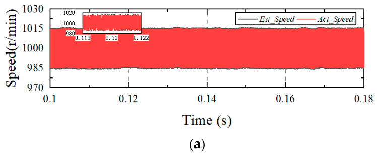
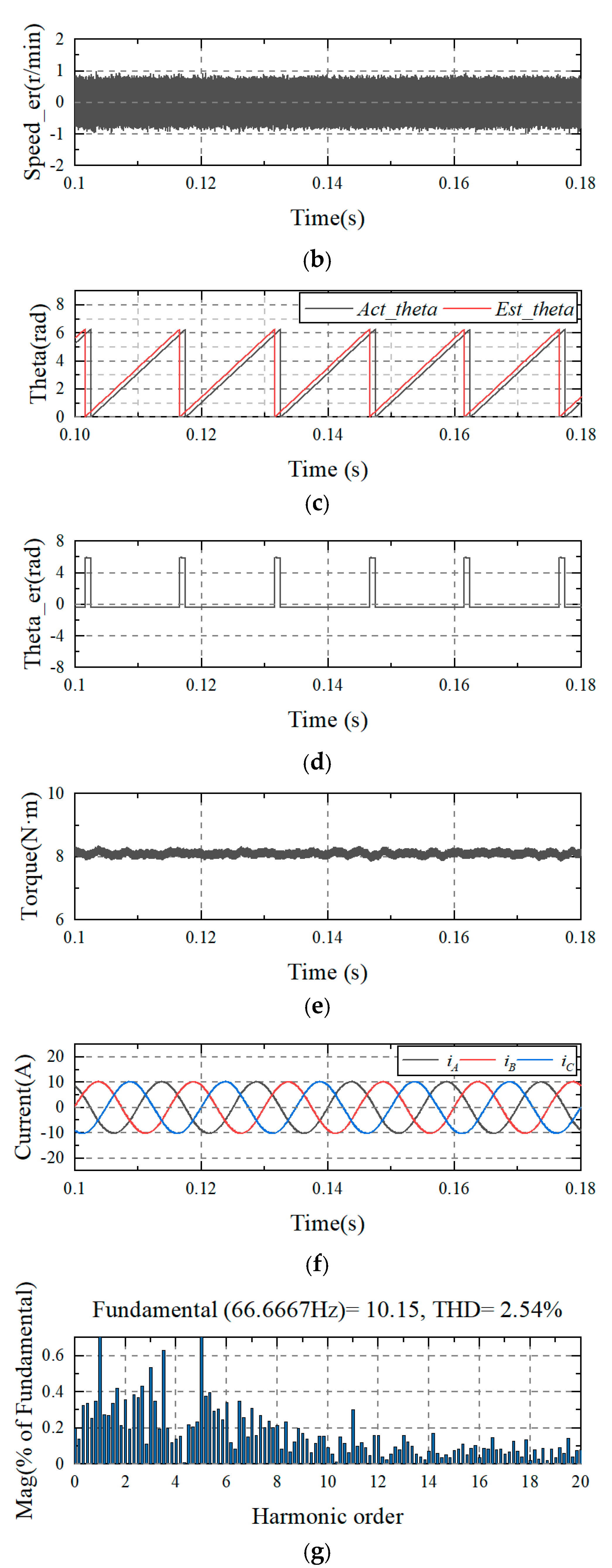
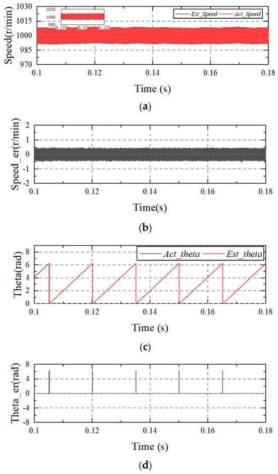
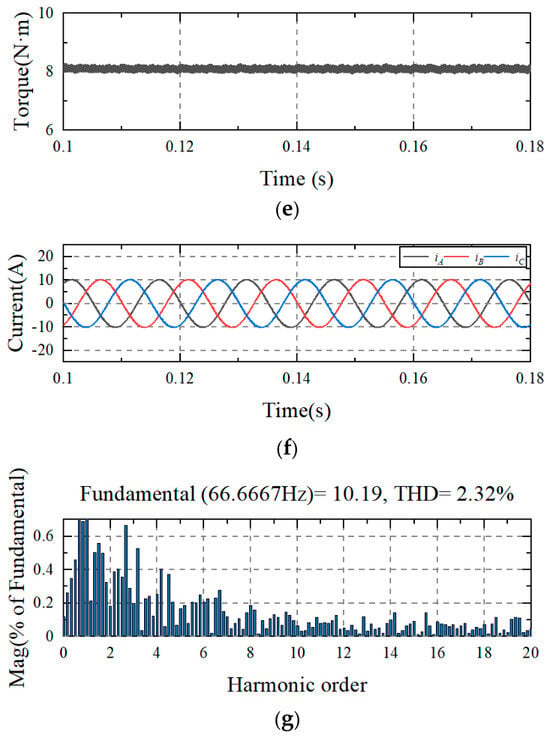
Steady-state performance was examined at the rated load of 8 N·m. After the motor stabilized at 1000 r/min, data from 0.10 s to 0.18 s were selected to compare STASMO and FTESMO in terms of estimation accuracy, chattering suppression capability, and current quality.

Figure 3 reports STASMO at 1000 r/min and rated load. The speed-estimation error is approximately ±0.8 r/min, while the estimated speed follows the actual-speed trajectory closely. The wider excursions in Figure 3a reflect the closed-loop speed ripple. The reported A-phase current THD is 2.54%, providing a quantitative measure of the current waveform quality.

Figure 3. Reported steady-state results of STASMO under rated-load operation at 1000 r/min. (a) Speed; (b) speed error; (c) rotor angle; (d) angle error; (e) torque; (f) phase current; (g) total harmonic distortion (THD) analysis.

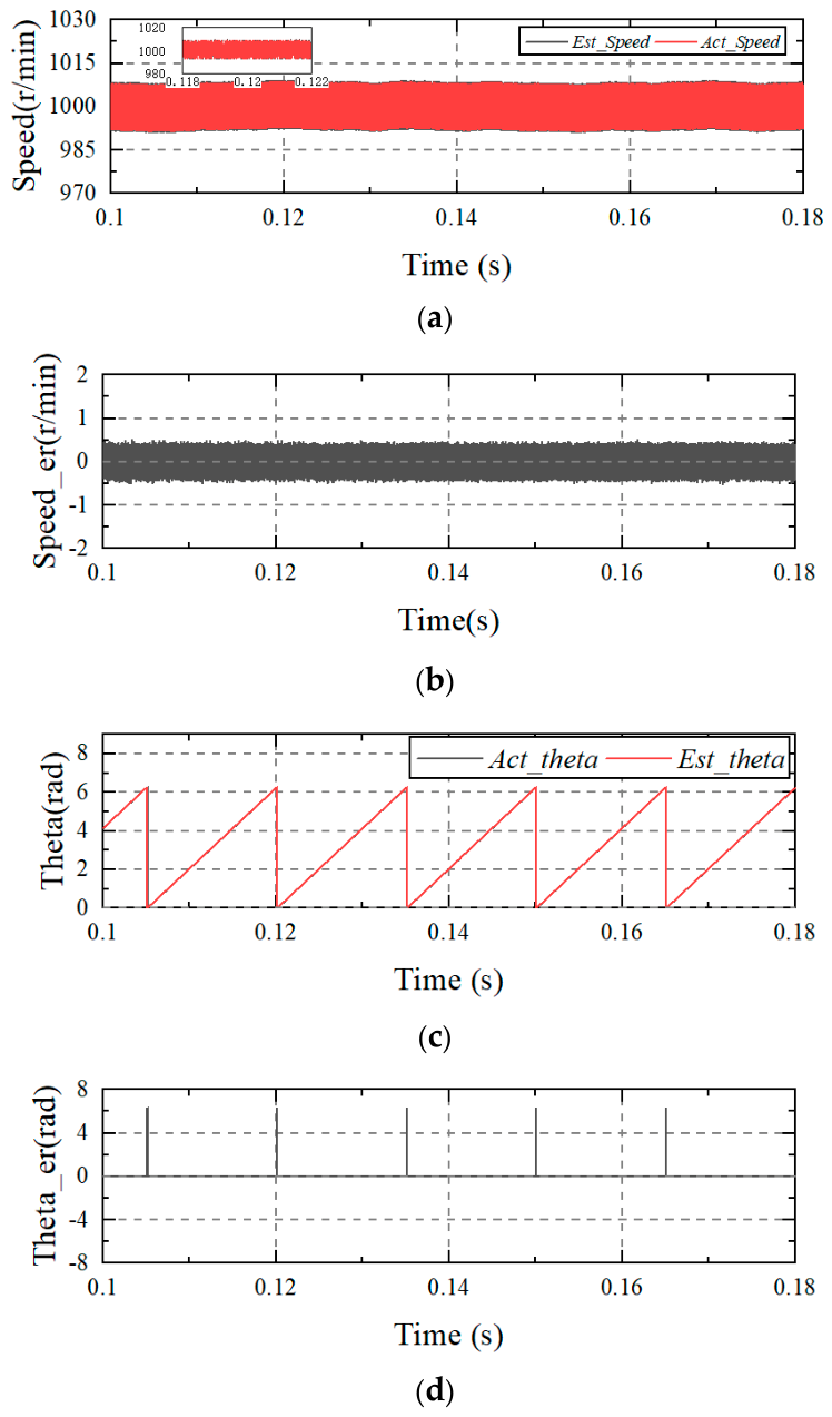
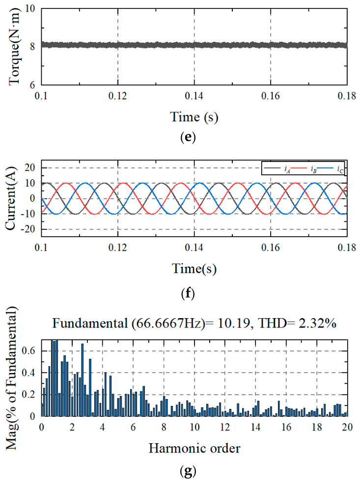
Figure 4 reports a speed-estimation error of approximately ±0.5 r/min and an A-phase current THD of 2.32%, compared with 2.54% for STASMO. Angle accuracy is assessed using the shortest signed circular difference, in electrical degrees, with estimated minus reference as the positive convention. All samples, including angle-wrapping samples, are retained. RMSE is the square root of the mean of the squared circular errors within the stated window; peak error is the maximum absolute circular error in that same window. No reset-spike exclusion or mean-bias removal is used in these definitions. The angle-error panels in Figure 3 and Figure 4 display differences between wrapped angles in radians; the full-cycle jumps in these panels must not be interpreted as the circular-error metrics defined above. For the reported FFT analysis, the A-phase current is evaluated from 0.09 s over six fundamental periods at 66.6667 Hz, corresponding to 0.09–0.18 s. The spectrum is displayed up to the twentieth harmonic, approximately 1333.33 Hz, whereas the Max THD frequency setting is Nyquist frequency. The displayed spectral limit therefore differs from the THD integration limit. The THD percentages describe the supplied records. The reported THD values are calculated using the same FFT window and frequency settings for both observers.

Figure 4. Reported steady-state results of FTESMO under rated-load operation at 1000 r/min. (a) Speed; (b) speed error; (c) rotor angle; (d) angle error; (e) torque; (f) phase current; (g) total harmonic distortion (THD) analysis.

4.2. Dynamic Speed-Reversal Experiment

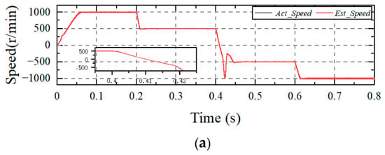
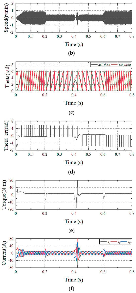
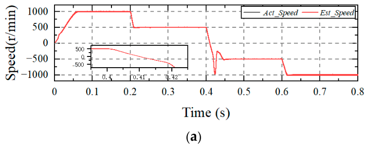
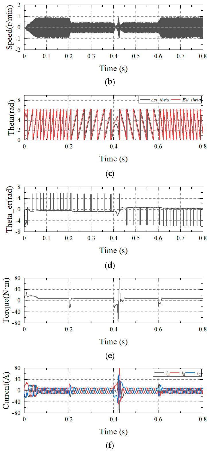
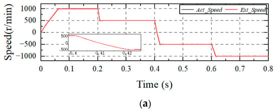
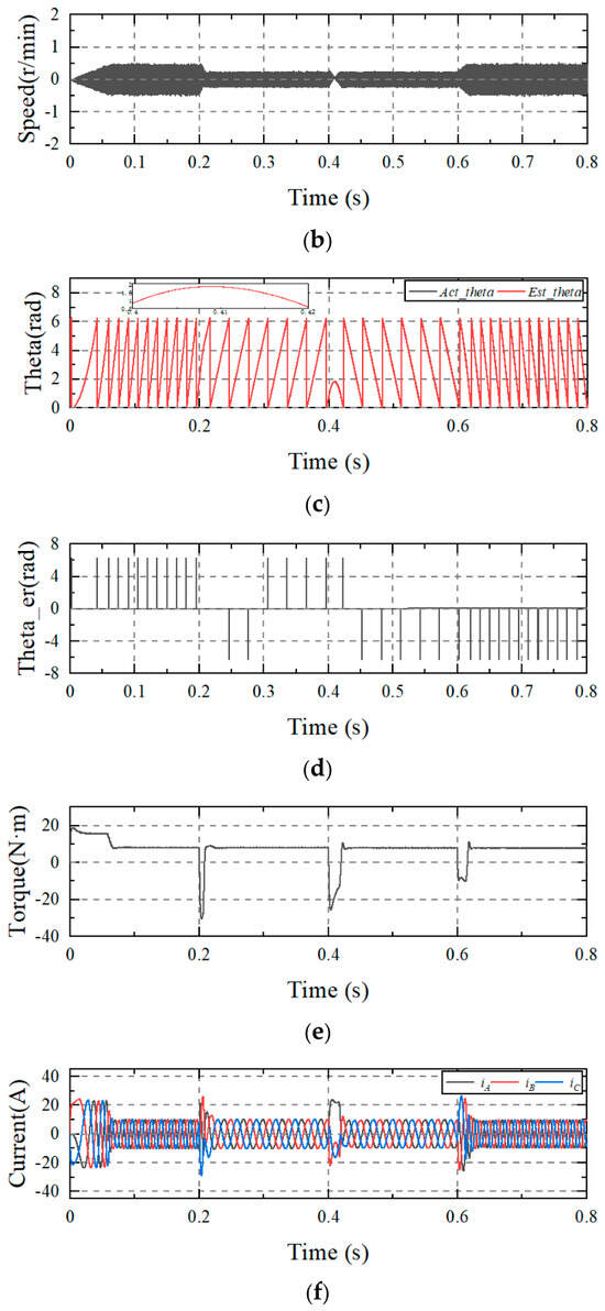
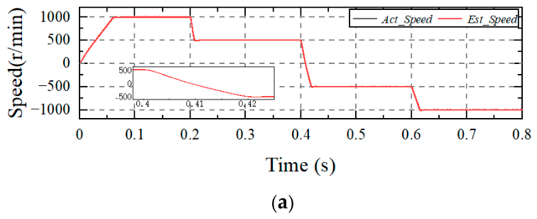
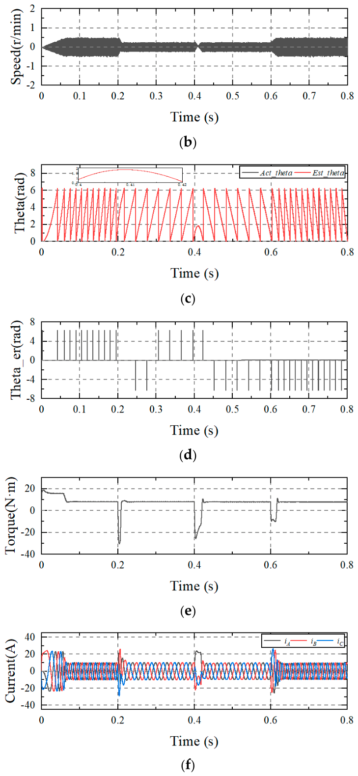
The rated-load speed-reversal records in Figure 5 and Figure 6 are compared over 0.8 s. The reversal transient is evaluated over 0.35–0.50 s, including the change in direction near 0.4 s. The torque traces in Figure 5, Figure 6 and Figure 7 represent calculated electromagnetic-torque obtained from the d- and q-axis current components and the motor parameters using the electromagnetic-torque expression in Section 2.1. The motor has a short-duration torque capability of 150 N·m, which exceeds the calculated electromagnetic torque peaks during speed reversal, while the continuous rated torque is 8 N·m. The circular-angle error is defined as the shortest signed angular difference between the estimated and actual electrical rotor positions, with estimated minus actual taken as positive, and is expressed in electrical degrees between −180° and +180°. This definition avoids artificial full-cycle jumps at the angle-wrapping boundary. Peak errors are the maximum absolute values within the stated interval; current peaks are taken across all three phases.

$$e_{\theta }={\displaystyle \frac{180}{\pi }}\mathrm{atan}2\left[\sin \left({\widehat{\theta }}_e-{\theta }_e\right),\cos \left({\widehat{\theta }}_e-{\theta }_e\right)\right]$$

(31)

Figure 5. Dynamic response of STASMO under rated-load speed-reversal operation. (a) Speed; (b) speed error; (c) rotor angle; (d) wrapped-angle difference in radians; (e) calculated electromagnetic torque; (f) phase current.

Figure 6. Dynamic response of FTESMO under rated-load speed-reversal operation. (a) Actual speed (gray solid) and estimated speed (red dashed); (b) speed-estimation error; (c) actual electrical rotor angle (gray solid) and estimated electrical rotor angle (red dashed); (d) wrapped-angle difference in radians; (e) calculated electromagnetic torque; (f) phase current.

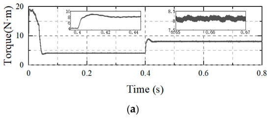
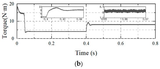
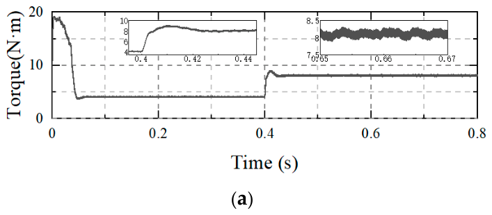
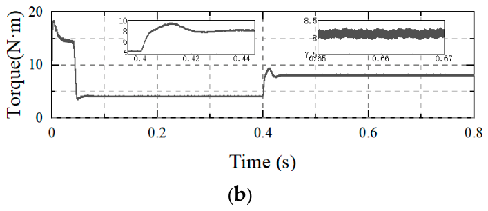
Figure 7. Calculated electromagnetic-torque response to a torque-reference step from 4 N·m to 8 N·m at 0.4 s. (a) STASMO; (b) FTESMO.

For N samples in a specified evaluation window, denote the sampled circular difference in (31) by the indexed angle-error symbol used below. The signed arithmetic mean in (32) measures directional bias within that window.

$${\overline{\epsilon }}_{\theta }={\displaystyle \frac{1}{N}}{\displaystyle \sum _{k=1}^N{\epsilon }_{\theta ,k}}$$

(32)

The root-mean-square angle error in (33) combines the signed bias and the variation about it. All samples, including those at angle wrapping, are retained.

$${\mathrm{RMSE}}_{\theta }=\sqrt{{\displaystyle \frac{1}{N}}{\displaystyle \sum _{k=1}^N{\epsilon }_{\theta ,k}^2}}$$

(33)

The maximum absolute circular-angle error in (34) measures the largest deviation within the same window. All three statistics are expressed in electrical degrees.

ε_θ,pk = max_k|ε_θ,k|

(34)

During the speed-reversal test in Figure 5, STASMO maintains basic tracking during the steady-state intervals but exhibits pronounced transient tracking degradation near the change in direction. Over 0.35–0.50 s, the peak speed-estimation error and circular-angle error are approximately 4.74 r/min and 129.90 electrical degrees, respectively. The calculated torque reaches +127.71 N·m at 0.427183 s and −74.02 N·m at 0.420682 s; the maximum absolute phase current is 93.05 A. The excursions are brief features of the reversal record rather than continuous operation at these levels. The calculated positive peak is below the confirmed short-duration motor torque capability of 150 N·m.

In Figure 6a,c, the actual quantities are shown by gray solid lines and the estimates by red dashed lines. Over 0.35–0.50 s, the actual and estimated speeds coincide to numerical precision, demonstrating close speed-estimation tracking during the reversal transient. Rotor-angle accuracy is evaluated using the shortest signed circular difference, which removes artificial full-cycle jumps caused by angle wrapping while retaining all sampled data. The maximum absolute circular-angle error is 0.98 electrical degrees over 0.35–0.50 s and 3.62 electrical degrees over the complete 0–0.80 s record. During the reversal interval, the calculated torque ranges from −25.58 to +10.83 N·m, and the absolute phase-current peak is 24.13 A. These transient extrema are smaller than those of the STASMO record.

The signed mean errors quantify the rotor-angle offset within the four operating windows, while the RMSE values characterize the combined effects of offset and fluctuation. FTESMO substantially reduces both the mean and RMS angle errors relative to STASMO at the four tested speed levels. Section 4.4 further compares the original FTESMO residual-voltage outputs with the corresponding reference components, providing an additional evaluation of the signal-recovery accuracy.

4.3. Torque-Reference Step Test

Figure 7 evaluates the calculated electromagnetic-torque response to a torque-reference command change from 4 N·m to 8 N·m at 0.4 s, providing an evaluation of torque-reference tracking. This test is distinct from the speed-reversal tests in Figure 5 and Figure 6.

The quantitative comparison in Figure 7 uses the unfiltered torque samples and identical evaluation windows for both observers. The initial and final response levels are defined by the means over 0.30–0.39 s and 0.60–0.80 s, respectively. Rise time is measured between the first crossings of 10% and 90% of the change between those means after the torque-reference step at 0.4 s. The rise times are 2.401 ms for STASMO and 2.954 ms for FTESMO. Their post-step torque peaks are 9.111 and 9.547 N·m, respectively. The corresponding overshoots above the final mean are 1.006 and 1.442 N·m. Normalized by the change between the initial and final means, these overshoots are 25.16% for STASMO and 36.04% for FTESMO.

Steady-state torque ripple is defined as half the peak-to-peak range within a specified window. Before the step, over 0.20–0.35 s, it is 0.181 N·m for STASMO and 0.148 N·m for FTESMO. After the step, over 0.60–0.80 s, the corresponding values are 0.255 and 0.180 N·m, equivalent to peak-to-peak variations of 0.509 and 0.360 N·m. In the latter window, STASMO ranges from 7.843 to 8.352 N·m with a mean of 8.105 N·m, whereas FTESMO ranges from 7.926 to 8.286 N·m with a mean of 8.106 N·m. Based on the unrounded values, FTESMO reduces the post-step torque half-range by 29.24% in the supplied record. These sample-based values replace the earlier approximate ripple levels of ±0.3 and ±0.05 N·m. The supported conclusion is a smaller steady-state torque ripple for FTESMO under the tested torque-reference step condition.

In the torque-reference test, FTESMO reduces the post-step steady-state torque half-range from 0.255 N·m to 0.180 N·m, corresponding to a reduction of 29.24%. Both observers exhibit millisecond-level transient response, while the principal improvement of FTESMO in this experiment is reflected in the reduced steady-state torque fluctuation.

4.4. Back-EMF Waveform Comparison

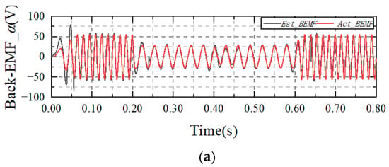
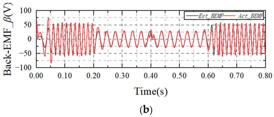
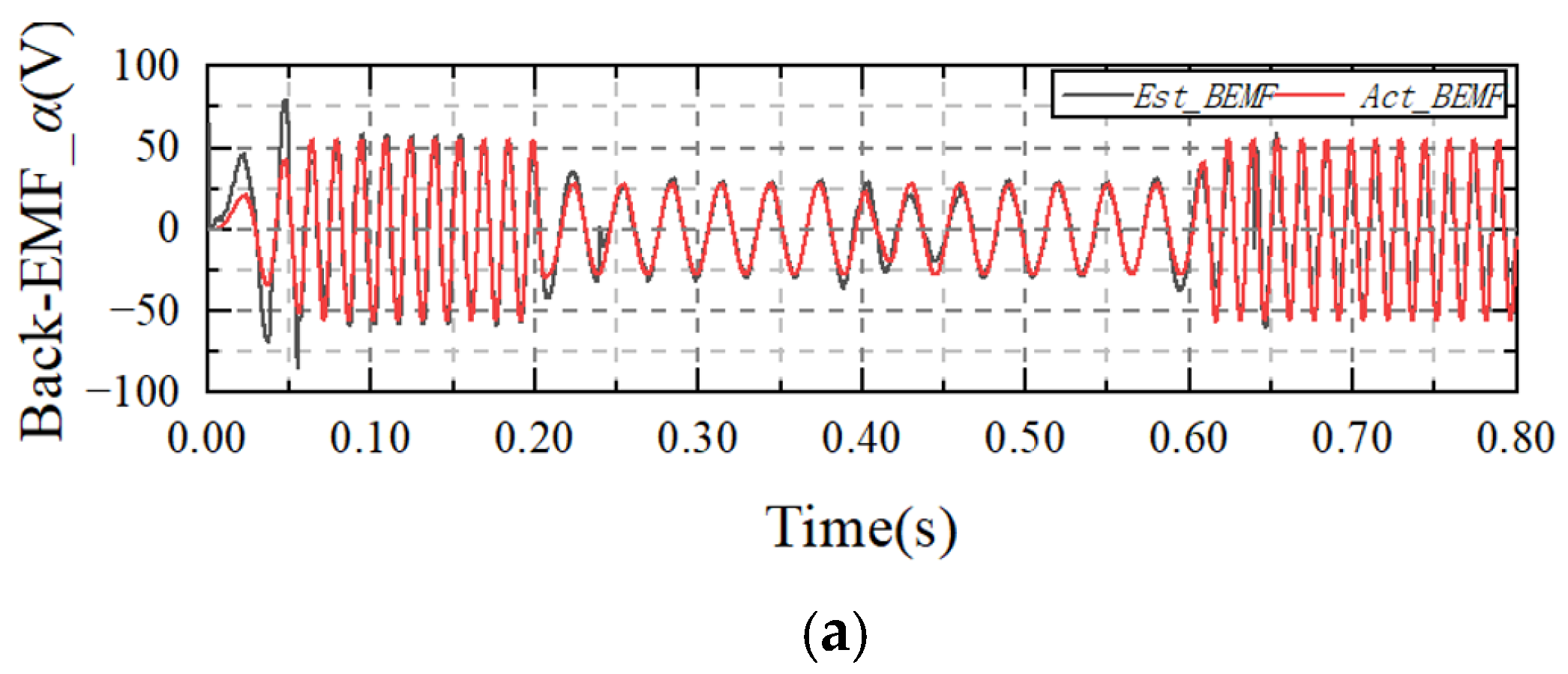
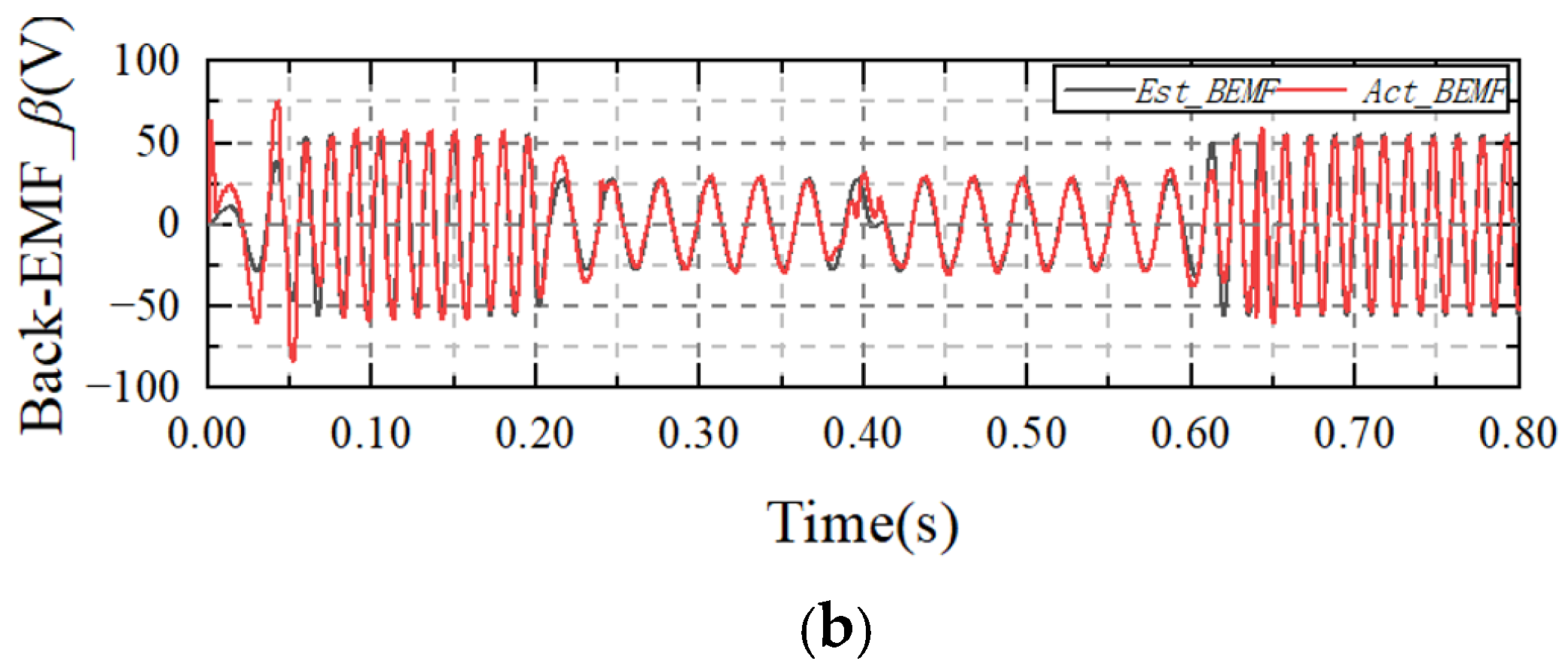
Figure 8 compares the reference back-EMF components with the original FTESMO outputs in the stationary alpha-beta frame over the complete 0–0.8 s record. Figure 8a,b show the alpha- and beta-axis components, respectively. No reference-assisted phase alignment or amplitude correction is applied to the displayed observer outputs. Gray solid lines denote the observer estimates, and red dashed lines denote the reference components.

Figure 8. Comparison of reference back-EMF components and original FTESMO outputs over 0–0.8 s. (a) Alpha-axis component; (b) beta-axis component.

Figure 8 provides a direct comparison between the FTESMO residual-voltage estimates and the corresponding reference components over the complete 0–0.8 s record. The estimated alpha- and beta-axis components reproduce the principal waveform evolution during the tested speed transitions. Together with the circular-angle statistics in Section 4.2, these results demonstrate effective residual-voltage reconstruction and rotor-position estimation under the investigated operating conditions.

4.5. Component-Ablation Comparison

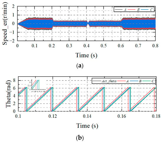
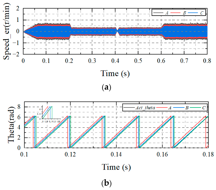
Figure 9 compares three configurations to examine the linear reaching term and the continuous smoothing mechanism separately. Group A removes the linear term k1s while retaining the other observer terms. Group B retains the linear and fractional-power feedback but replaces the smooth switching function by the signum function. Group C is the complete FTESMO. The other parameters and test settings are unchanged across the three groups. Figure 9a shows the speed-estimation error over 0–0.8 s, and Figure 9b compares the electrical rotor angles over 0.10–0.18 s, including a local view near 0.12 s.

Figure 9. Component-ablation comparison. A: linear reaching term removed; B: smooth switching replaced by signum; C: complete FTESMO. (a) Speed-estimation error: A, gray; B, red; C, blue. (b) Electrical rotor angle: reference, gray; A, red; B, blue; C, green.

Figure 9a shows that the complete FTESMO exhibits the narrowest speed-estimation-error envelope, whereas removing the linear reaching term produces the largest error fluctuation and replacing the smooth switching function with signum injection gives an intermediate response. This ordering demonstrates the contribution of the linear reaching term to error convergence and the contribution of the continuous smoothing function to steady-state estimation quality.

Figure 9b further shows differences in rotor-angle tracking among the three configurations. Group A exhibits the largest angular displacement from the reference trajectory, whereas Groups B and C remain closer to the reference. The combined speed-error and rotor-angle comparisons demonstrate that the linear reaching term and continuous smoothing mechanism provide complementary contributions. Their combination in the complete FTESMO yields the best overall estimation performance among the three tested configurations.

5. Conclusions

An exponential sliding-mode observer with a continuous boundary layer has been developed for position-sensorless IPMSM drives. The proposed observer combines a saliency-aware residual-voltage model with linear and fractional-power current-error feedback and a continuous piecewise-quadratic switching function. The theoretical analysis establishes finite-time convergence of the ideal reaching law and further derives ultimate-error bounds, boundary-layer invariance conditions, and a finite entry-time condition for the continuous observer under bounded forcing.

Experimental comparisons demonstrate improved estimation performance relative to STASMO. At rated load and 1000 r/min, the speed-estimation-error range decreases from approximately ±0.8 r/min to ±0.5 r/min, while the A-phase current THD decreases from 2.54% to 2.32%. During speed reversal, FTESMO substantially reduces the rotor-angle estimation errors at the tested speed levels. In the torque-reference experiment, the post-step steady-state torque half-range decreases from 0.255 N·m to 0.180 N·m, corresponding to a reduction of 29.24%. The residual-voltage waveform comparison further verifies effective signal reconstruction during the tested dynamic transitions.

The component-ablation comparison shows that removal of the linear reaching term increases the speed-estimation-error envelope, whereas replacing the continuous smoothing function with signum injection produces an intermediate response. These results demonstrate the complementary contributions of the linear reaching term and continuous smoothing mechanism and confirm the effectiveness of the complete FTESMO for position-sensorless IPMSM operation under the investigated steady-state and dynamic conditions.

References

- Wang, D.; Xu, S.; Li, Y.; Wang, B.; Wang, X.; Nie, J.; Wang, X. Sensorless Control Impact on Electromagnetic Vibrations and Acoustic Noises in Interior Permanent Magnet Synchronous Machines. IEEE Trans. Transp. Electrif. 2025, 11, 416–425. [Google Scholar] [CrossRef] [Scilit]
- Tian, B.; Li, Y.; Hu, J.; Wang, G.; Molinas, M.; Zhang, G.; Wang, K.; Zhang, Z. A Wide Speed Range Sensorless Control for Three-Phase PMSMs Based on a High-Dynamic Back EMF Observer. IEEE Trans. Transp. Electrif. 2025, 11, 4336–4349. [Google Scholar] [CrossRef] [Scilit]
- Chen, Z.; Jing, H.; Wang, X.; Luo, D.; Wang, X.; Fang, G.; Zhao, H.; Xiao, D. Selective Harmonic Elimination and Dynamic Enhancement in Magnetic-Characteristic-Free Sensorless Control of SRM Drives at High Speeds. IEEE Trans. Power Electron. 2024, 39, 5339–5348. [Google Scholar] [CrossRef] [Scilit]
- Bi, G.; Zhang, G.; Wang, Q.; Ding, D.; Li, B.; Wang, G.; Xu, D. High-Frequency Injection Angle Self-Adjustment Based Online Position Error Suppression Method for Sensorless PMSM Drives. IEEE Trans. Power Electron. 2023, 38, 1412–1417. [Google Scholar] [CrossRef] [Scilit]
- Naderian, M.; Markadeh, G.A.; Karimi-Ghartemani, M.; Mojiri, M. Improved Sensorless Control Strategy for IPMSM Using an ePLL Approach with High-Frequency Injection. IEEE Trans. Ind. Electron. 2024, 71, 2231–2241. [Google Scholar] [CrossRef] [Scilit]
- Wang, L.; Miao, H. Novel adaptive extended state observer method of active disturbance rejection control for sensorless IPMSMs based on high-frequency square wave injection. J. Power Electron. 2026, 26, 574–585. [Google Scholar] [CrossRef] [Scilit]
- Liu, P.; Liu, D.; Shen, Y.; Liu, A.; Yang, X.; Zhao, J. Full speed range position-sensorless compound control scheme for PMSMs. J. Power Electron. 2022, 22, 1302–1312. [Google Scholar] [CrossRef] [Scilit]
- Woldegiorgis, A.T.; Ge, X.; Wang, H.; Zuo, Y. An Active Flux Estimation in the Estimated Reference Frame for Sensorless Control of IPMSM. IEEE Trans. Power Electron. 2022, 37, 9047–9060. [Google Scholar] [CrossRef] [Scilit]
- Ge, Y.; Song, W.; Yang, Y.; Wheeler, P. A Polar-Coordinate-Multisignal-Flux-Observer-Based PMSM Non-PLL Sensorless Control. IEEE Trans. Power Electron. 2023, 38, 10579–10583. [Google Scholar] [CrossRef] [Scilit]
- Li, B.; Zou, J.; Xu, Y.; Li, S.; Jin, S. Sensorless Control of DTP-SynRM with Hybrid Flux Observer and Disturbance Observer Considering Magnetic Saturation and Cross-Coupling Effect. IEEE Trans. Power Electron. 2025, 40, 12295–12308. [Google Scholar] [CrossRef] [Scilit]
- Zuo, Y.; Lai, C.; Iyer, K.L.V. A Review of Sliding Mode Observer Based Sensorless Control Methods for PMSM Drive. IEEE Trans. Power Electron. 2023, 38, 11352–11367. [Google Scholar] [CrossRef] [Scilit]
- Yuan, Q.; Ma, Y.; Huang, Y.; Xia, K.; Yu, Y. Adaptable sliding mode observer-based sensorless control with harmonic current compensation for dual three-phase PMSMs. J. Power Electron. 2024, 24, 1889–1898. [Google Scholar] [CrossRef] [Scilit]
- Chen, S.; Ding, W.; Hu, R.; Wu, X.; Shi, S. Sensorless Control of PMSM Drives Using Reduced Order Quasi Resonant-Based ESO and Newton–Raphson Method-Based PLL. IEEE Trans. Power Electron. 2023, 38, 229–244. [Google Scholar] [CrossRef] [Scilit]
- Liu, Z.-H.; Nie, J.; Wei, H.-L.; Chen, L.; Li, X.-H.; Lv, M.-Y. Switched PI Control Based MRAS for Sensorless Control of PMSM Drives Using Fuzzy-Logic-Controller. IEEE Open J. Power Electron. 2022, 3, 368–381. [Google Scholar] [CrossRef] [Scilit]
- Pasqualotto, D.; Rigon, S.; Zigliotto, M. Sensorless Speed Control of Synchronous Reluctance Motor Drives Based on Extended Kalman Filter and Neural Magnetic Model. IEEE Trans. Ind. Electron. 2023, 70, 1321–1330. [Google Scholar] [CrossRef] [Scilit]
- Sang, Y.; Wu, Z.; Fan, Y. An adaptive extended Kalman filter observer-for permanent magnet synchronous motor position sensorless control systems. Sci. Rep. 2025, 15, 11605. [Google Scholar] [CrossRef] [Scilit]
- Kumar, S.; Singh, B. Sensorless Adaptive SMO with Mixed Order Generalized Integrator Based Improved QPLL PMSM Drive for LEV Application. IEEE Trans. Ind. Appl. 2024, 60, 9100–9110. [Google Scholar] [CrossRef] [Scilit]
- Sun, H.; Zhang, X.; Liu, X.; Su, H. Adaptive Robust Sensorless Control for PMSM Based on Improved Back EMF Observer and Extended State Observer. IEEE Trans. Ind. Electron. 2024, 71, 16635–16643. [Google Scholar] [CrossRef] [Scilit]
- Wang, B.; Shao, Y.; Yu, Y.; Dong, Q.; Yun, Z.; Xu, D. High-Order Terminal Sliding-Mode Observer for Chattering Suppression and Finite-Time Convergence in Sensorless SPMSM Drives. IEEE Trans. Power Electron. 2021, 36, 11910–11920. [Google Scholar] [CrossRef] [Scilit]
- Chen, L.; Jin, Z.; Shao, K.; Wang, H.; Wang, G.; Iu, H.H.-C.; Fernando, T. Sensorless Fixed-Time Sliding Mode Control of PMSM Based on Barrier Function Adaptive Super-Twisting Observer. IEEE Trans. Power Electron. 2024, 39, 3037–3051. [Google Scholar] [CrossRef] [Scilit]
- Wang, H.; Jiao, T.; Xing, X.; Yang, Y. Speed Regulation of PMSM Systems Based on a New Sliding Mode Reaching Law. IEEE Access 2024, 12, 24062–24070. [Google Scholar] [CrossRef] [Scilit]
- Zou, X.; Ding, H.; Li, J. Sensorless Control Strategy of Permanent Magnet Synchronous Motor Based on Fuzzy Sliding Mode Controller and Fuzzy Sliding Mode Observer. J. Electr. Eng. Technol. 2022, 18, 2355–2369. [Google Scholar] [CrossRef] [Scilit]
Disclaimer/Publisher’s Note: The statements, opinions and data contained in all publications are solely those of the individual author(s) and contributor(s) and not of MDPI and/or the editor(s). MDPI and/or the editor(s) disclaim responsibility for any injury to people or property resulting from any ideas, methods, instructions or products referred to in the content. |
© 2026 by the authors. Licensee MDPI, Basel, Switzerland. This article is an open access article distributed under the terms and conditions of the Creative Commons Attribution (CC BY) license.