A Cross-Session Assessment of the 2X Response to Dial-Indicator-Verified Motor-Base Displacement: An Assembly-Related Transfer-Path Interpretation

Abstract

The second rotational-frequency component (2X) is commonly used as a misalignment-related vibration feature, but its amplitude stability after reassembly remains uncertain. This exploratory study compares three independent normal-bearing reassembly sessions. Six horizontal motor-base displacement settings were imposed by an adjustment screw, rechecked using a dial indicator, and followed by three waveform acquisitions each. These settings are not direct measurements of shaft-center offset. Horizontal housing vibration was analyzed at twice a vibration-derived rotational-frequency estimate. The session-mean tracked-bin responses differed, but the inferred cross-setting trend showed sensitivity to the harmonic-amplitude estimator. A predefined nonlinear rotor–bearing–foundation model separately tested whether an equivalent support-state change alters transfer gain under controlled 20 Hz forcing. Within its parameter scan it changed gain and response sensitivity, without fitting sessions or reproducing their observed curve shapes. The three-session comparison is descriptive, and missing calibration and uncertainty records limit quantitative transfer. The findings motivate joint documentation of displacement setting, assembly, measurement conditions, and harmonic estimation before using absolute 2X amplitude across sessions.

1. Introduction

Shaft misalignment can alter the fundamental rotational-frequency component and its harmonics. Dynamic bearing misalignment, coupling misalignment, and multi-support rotor models associate 2X and higher components with contact and excitation changes [1,2,3,4]. Bearing tilt and combined misalignment can also change contact-load distribution [5,6]. These observations motivate using 2X as a diagnostic feature. They do not establish that an absolute 2X amplitude gives a transferable measure of geometric misalignment across different assembly realizations.

Controlled single-rig studies are useful for examining response to imposed settings. Lal investigated applied misalignment, orbital response, and repeat statistics on a rotor–bearing rig [7]. Coupling–bearing models examined force and harmonic responses under different configurations [2,5]. Local defects and cage damage introduce further contact-related sources of harmonic variation [8,9]. The relevant question here is narrower than general misalignment diagnosis: how do recorded 2X responses vary among independently reassembled sessions under nominally matched conditions?

A measured housing response combines excitation with transmission through the machine and its measurement chain. Source–path–receiver methods provide a framework for separating these roles [10,11]. Bearing-housing studies show that interfaces and sensor location can affect measured transmissibility [12]. Preload can affect modal properties [13,14]; fit clearance, housing stiffness, and pedestal conditions can affect vibration and stability [15,16,17]. Support and foundation models likewise demonstrate changes in resonant response [18,19,20,21,22]. These studies support candidate mechanisms, not specific claims about what changed during the present reassemblies.

Repeated acquisitions within one session and independently reassembled sessions represent different replication levels. Bearing-quality and condition-monitoring studies discuss refitting, measurement position, and measurement-system variation [23,24]. A separate rail-model study demonstrates sensitivity to accelerometer attachment in non-destructive testing [25]; it is indirect evidence for this rotor rig, not a reassembly experiment on misalignment. Cross-session misalignment diagnosis has also been studied for classifier generalization [26]; that objective differs from examining dimensional response curves. The cross-session stability of the 2X–misalignment relationship remains insufficiently characterized, particularly where nominal settings, within-session repeats, and reassembly are distinguished.

This paper presents an exploratory cross-session case study of three independently reassembled normal-bearing sessions, S4–S6. Each has six horizontal motor-base displacement settings, rechecked with a dial indicator, and three repeated acquisitions at each setting. The primary metric is the horizontal ch2 vibration-spectrum amplitude at twice a record-specific spectral estimate of rotational frequency. A verified motor-base displacement is not a direct measurement of shaft-center offset or residual angle. Missing instrument-calibration and uncertainty records, together with only three sessions, prevent a calibrated shaft-misalignment severity relationship or a population-level reproducibility claim.

The contribution has three bounded parts: a descriptive comparison of the observed session-mean curves; a reproducible check that a predefined support-state proxy changes response sensitivity in a nonlinear model with monotonic equivalent forcing; and an assessment of the limits of linking the two. Existing waveforms are reanalyzed to recover the processing chain, actual frequency range, and a consistently defined local spectral background. The numerical checks distinguish stationary linearization, finite nonlinear response, and rolling-element configuration. Neither the model nor the literature is used to assign S4, S5, or S6 to an identified physical stiffness.

2. Reproducible Reduced-Order Model

2.1. Coordinates, Scope, and Force Balance

The archived script simulation_v6_assembly_scan_FROZEN_20260905.m defines a transverse six-degree-of-freedom model,

$$\mathit{q}={(x_i,y_i,x_o,y_o,x_f,y_f)}^{\mathrm{T}},$$

(1)

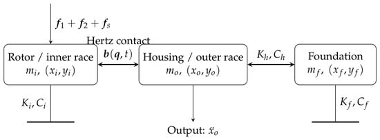
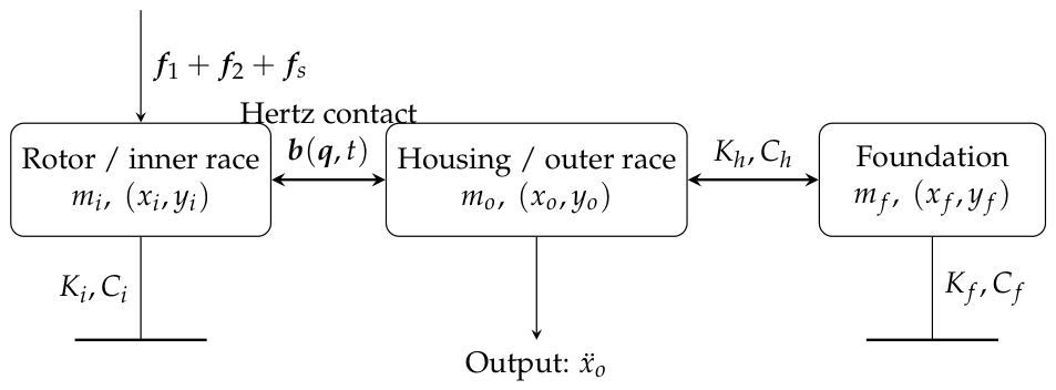
where i, o, and f denote the equivalent rotor/inner race, housing/outer race, and foundation. The model has no explicit second shaft centerline, axial motion, torsion, or continuous housing modes. Figure 1 shows the retained coordinates and connections. Parameters are model assumptions unless explicitly identified otherwise in Supplementary Table S1; they were not identified from S4–S6.

Figure 1. Connections retained by the six-DOF model. Each block has an $x,y$ coordinate pair. Contact acts between rotor and housing; housing and foundation are coupled by $K_h,C_h$. The rotor and foundation have separate grounded stiffness/damping. The illustrated springs and dampers denote equivalent lumped model coefficients rather than literal physical components at the shown locations. Housing x is horizontal, conceptually consistent with experimental ch2, without a calibrated amplitude mapping.

With ${\mathit{u}}_i={(x_i,y_i)}^{\mathrm{T}}$, ${\mathit{u}}_o={(x_o,y_o)}^{\mathrm{T}}$, ${\mathit{u}}_f={(x_f,y_f)}^{\mathrm{T}}$, the implemented equations are

$$\begin{array}{cc}\hfill m_i{\ddot{\mathit{u}}}_i+{\mathit{C}}_i{\dot{\mathit{u}}}_i+{\mathit{K}}_i{\mathit{u}}_i+\mathit{b}& ={\mathit{f}}_1+{\mathit{f}}_2+{\mathit{f}}_s,\hfill \\ \hfill m_o{\ddot{\mathit{u}}}_o+{\mathit{C}}_h({\dot{\mathit{u}}}_o-{\dot{\mathit{u}}}_f)+{\mathit{K}}_h({\mathit{u}}_o-{\mathit{u}}_f)-\mathit{b}& =\mathbf{0},\hfill \\ \hfill m_f{\ddot{\mathit{u}}}_f+{\mathit{C}}_f{\dot{\mathit{u}}}_f+{\mathit{K}}_f{\mathit{u}}_f-{\mathit{C}}_h({\dot{\mathit{u}}}_o-{\dot{\mathit{u}}}_f)-{\mathit{K}}_h({\mathit{u}}_o-{\mathit{u}}_f)& =\mathbf{0}.\hfill \end{array}$$

(2)

All two-dimensional coefficient matrices in Equation (2) are diagonal. Thus,

$$\mathit{M}\ddot{\mathit{q}}+\mathit{C}\dot{\mathit{q}}+\mathit{K}\mathit{q}+{\mathit{F}}_b(\mathit{q},t)={\mathit{F}}_1\left(t\right)+{\mathit{F}}_m({\delta }_m,t)+{\mathit{F}}_s,$$

(3)

with $\mathit{M}=diag(m_i,m_i,m_o,m_o,m_f,m_f)$,

$$\mathit{K}=\left[\begin{array}{ccc}{\mathit{K}}_i& 0& 0\\ 0& {\mathit{K}}_h& -{\mathit{K}}_h\\ 0& -{\mathit{K}}_h& {\mathit{K}}_h+{\mathit{K}}_f\end{array}\right],\mathit{C}=\left[\begin{array}{ccc}{\mathit{C}}_i& 0& 0\\ 0& {\mathit{C}}_h& -{\mathit{C}}_h\\ 0& -{\mathit{C}}_h& {\mathit{C}}_h+{\mathit{C}}_f\end{array}\right],{\mathit{F}}_b=\left[\begin{array}{c}\mathit{b}\\ -\mathit{b}\\ \mathbf{0}\end{array}\right].$$

(4)

The first two entries of ${\mathit{F}}_1$, ${\mathit{F}}_m$, and ${\mathit{F}}_s$ are ${\mathit{f}}_1$, ${\mathit{f}}_2$, and ${\mathit{f}}_s={(0,-180)}^{\mathrm{T}}$ N, respectively; their remaining entries are zero. The constant force represents an assumed vertical preload. The code does not calculate $mg$ or apply separate gravitational loads to all three masses; no gravitational-acceleration parameter is present.

2.2. Rolling Contact and Excitation

For $j=1,\dots ,8$, define

$${\theta }_j\left(t\right)={\displaystyle \frac{2\pi (j-1)}{8}}+{\theta }_0+{\omega }_{c}t,{\mathit{n}}_j={(\cos {\theta }_j,\sin {\theta }_j)}^{\mathrm{T}},d_j={\mathit{n}}_j^{\mathrm{T}}({\mathit{u}}_i-{\mathit{u}}_o)-c_r.$$

(5)

The healthy-bearing contact force is exactly

$$\mathit{b}(\mathit{q},t)={\displaystyle \sum _{j=1}^8}{K}_H{\left[d_j\right]}_{+}^{3/2}{\mathit{n}}_j,{\left[d\right]}_{+}=\max (d,0),$$

(6)

where $K_H={10}^9$ N ${\mathrm{m}}^{-3/2}$ and $c_r=20\mathsf{\mu }$m. The clearance is the direct subtraction in $d_j$, not a separately inferred diametral clearance. The cage rate is prescribed as ${\omega }_c=0.397\Omega$. Bearing-defect depth is disabled in all reported cases. Contact stiffness therefore depends on both relative displacement and cage position. Contact/clearance and housing-boundary effects are physically motivated by prior bearing models [6,8,16,27,28,29,30]; these citations do not identify the numerical parameters of this rig.

The experimental quantity $\delta$ denotes the dial-indicator-verified horizontal motor-base displacement setting and is not implemented as an explicit geometric offset between two modeled shaft centerlines. The reduced-order model instead uses the separate parameter ${\delta }_m$, an equivalent-forcing input parameter that is neither a measured shaft-center offset nor a calibrated mapping from experimental $\delta$. It enters through an equivalent 2X excitation law used to test transfer sensitivity:

$$\eta =\min \left({\displaystyle \frac{|{\delta }_m|}{{\delta }_{m,\max }}},1\right),F_{2\mathrm{X},\mathrm{mis}}=K_{2\mathrm{X}}\eta +K_{2q}{\eta }^2,F_2=F_{2b}+F_{2\mathrm{X},\mathrm{mis}}.$$

(7)

Here, ${\delta }_{m,\max }=0.30$ mm, $K_{2\mathrm{X}}=3$ N, and $K_{2q}=F_{2b}=0$ N. Because $\eta$ is dimensionless, $K_{2\mathrm{X}}$ has units of force; the equivalent coefficient within the scanned interval is 10 N/mm. It is an assumed, non-identified forcing scale, not a measured coupling stiffness or a calibrated mapping from the experimental setting. The model grid is ${\delta }_m=0$, 0.05, 0.10, 0.15, 0.20, and 0.30 mm. The saturation outside $|{\delta }_m|=0.30$ mm is part of the code but is not reached by this scan. With these choices, the imposed 2X amplitude is strictly proportional to $|{\delta }_m|$ over the reported interval and vanishes at ${\delta }_m=0$.

$${\mathit{f}}_1=8\left[\begin{array}{c}\cos \Omega t\\ \sin \Omega t\end{array}\right]\mathrm{N},{\mathit{f}}_2=F_2\left[\begin{array}{c}\cos (2\Omega t+{\varphi }_2)\\ r_y\sin (2\Omega t+{\varphi }_2)\end{array}\right],r_y=0.5,{\varphi }_2={20}^{\circ }.$$

(8)

The background 1X force is independent of ${\delta }_m$. Hence a zero imposed misalignment force does not require a zero response at 20 Hz.

2.3. Support Proxy and Directional FRF

The dimensional foundation stiffness is $k_f=\alpha k_{f0}$ in both axes, with $k_{f0}={10}^5$ N/m and $\alpha \in \{0.55,0.75,1,1.25,1.50\}$. The symbol $\alpha =k_f/k_{f0}$ distinguishes the factor from dimensional stiffness. No experimental session is assigned an $\alpha$. All other physical coefficients remain fixed. The proxy tests one possible transfer mechanism; physical reassembly can also involve contact, fit, preload, damping, and measurement changes [5,13,15,17,18,22,31].

The static residual $\mathit{R}\left(\mathit{q}\right)$ is the right-hand force imbalance of Equation (2) at $t=0$, excluding the 1X and 2X harmonics. At its stationary solution ${\mathit{q}}_0$, ${\mathit{K}}_{\mathrm{eq}}=-\partial \mathit{R}/\partial \mathit{q}$ and ${\mathit{C}}_{\mathrm{eq}}=\mathit{C}$. With ${\mathit{e}}_j$ the jth coordinate basis vector,

$$\begin{array}{cc}\hfill \mathit{Z}\left(\omega \right)& =-{\omega }^2\mathit{M}+\mathrm{i}\omega {\mathit{C}}_{\mathrm{eq}}+{\mathit{K}}_{\mathrm{eq}},\hfill \\ \hfill H_{xx}& =-{\omega }^2{\mathit{e}}_3^{\mathrm{T}}{\mathit{Z}}^{-1}{\mathit{e}}_1,H_{xy}=-{\omega }^2{\mathit{e}}_3^{\mathrm{T}}{\mathit{Z}}^{-1}{\mathit{e}}_2,\hfill \\ \hfill H_a& =H_{xx}-\mathrm{i}{r}_y{H}_{xy},{\widehat{a}}_x=H_a{F}_2\exp \left(\mathrm{i}{\varphi }_2\right).\hfill \end{array}$$

(9)

Thus $H_a$ has units m ${\mathrm{s}}^{-2}$ N⁻¹ and $|{\widehat{a}}_x|$ has units m s⁻². The $-{\omega }^2$ factor converts displacement to acceleration, the force phasor acts on rotor coordinates 1 and 2, and coordinate 3 is housing x. Directional combination concerns the input force, not a combination of output axes. This stationary small-perturbation FRF is not a transfer function of the complete rotating nonlinear contact system.

2.4. Numerical Implementation

The archived calculations used MATLAB R2025b according to the retained execution record. Each case starts at $[{\mathit{q}}_0;\mathbf{0}]$. Static equilibrium minimizes ${\parallel \mathit{R}\parallel }_2^2$ with fminsearch, from six zeros, with TolX ${10}^{-11}$, TolFun ${10}^{-12}$, maximum 3000 iterations and 12,000 evaluations. A non-finite residual or ${\parallel \mathit{R}\parallel }_2>{10}^{-3}$ N triggers failure. Central differences with $h={10}^{-8}$ m form the tangent matrix, which is symmetrized. Dynamic integration uses ode15s, relative tolerance ${10}^{-6}$, scalar absolute tolerance ${10}^{-8}$ for the displacement/velocity state, and maximum step $5\times {10}^{-4}$ s. Dense output is sampled at 4000 Hz over 0–3 s. Housing acceleration is evaluated from the ODE right-hand side, not by differentiating displacement numerically.

The first second and the final endpoint are excluded, leaving 8000 samples over $1\le t<3$ s. The mean is removed and a periodic Hann window $w_n=0.5-0.5\cos (2\pi n/N)$ is applied. The retained positive-frequency amplitudes equal $2|FFT(wa\left)\right|/\sum w$. The code does not halve the DC or Nyquist endpoints; neither endpoint is used here. The primary simulated metric is the nearest bin to 20 Hz (exactly a bin at 0.5 Hz spacing). No additional detrending, digital filtering, interpolation, or band integration is applied. The 18–22 Hz maximum is stored separately. Exceptions are logged as solver failures; a successful return is not itself a convergence proof. The archived convergence routine changes both tolerances and duration, so its weak-background comparison also reflects a changed spectral window.

3. Numerical Investigation

3.1. Archived Scan and Numerical Checks

The reported scan remains the archived 30-case calculation: six input settings and five support factors. All 30 nonlinear cases have successful solver status and finite response metrics, with no logged solver failures. The preceding nine-case sanity matrix also completed. The optional linear_sanity check uses an isotropic bearing spring of $2.5\times {10}^5$ N/m, rather than the Hertz tangent matrix. Its input ratios 1:3:6 produced amplitude ratios 1:2.999942:5.999856, with maximum proportionality error 0.00241%. It verifies the force/FFT path but is distinct from the FRF consistency test below.

The maximum 0.0813% difference belongs to the earlier sanity convergence check. The full-scan file must be interpreted separately: the two tested nonzero-input cases ($\alpha =1$, ${\delta }_m=0.10$ mm; $\alpha =1.5$, ${\delta }_m=0.30$ mm) differ by 0.00438% and 0.00349%, respectively, between the archived settings. At $\alpha =0.55$, ${\delta }_m=0$, the weak 18–22 Hz band maximum changes from 0.00339690 to 0.00375596 m s⁻² (10.57%), while its bin changes from 22 to 21.667 Hz. Because the second setting also extends the retained record from 2 to 3 s, this is not an isolated solver-error estimate. It does not establish convergence of the zero-input band maximum. Fixed 20 Hz amplitudes and band maxima are therefore kept distinct.

3.2. Linear FRF Consistency and the Low-Stiffness Path

At $\alpha =0.55$ and ${\delta }_m=0.30$ mm, the imposed 2X force is 3 N. The archived MATLAB diagnostic, using identical $\mathit{M}$, ${\mathit{C}}_{\mathrm{eq}}$, ${\mathit{K}}_{\mathrm{eq}}$, input directions, phase, frequency, and output coordinate, gave

$$\begin{array}{cc}\hfill A_{2,\mathrm{FRF}}& =4.98771783621\times {10}^{-18}\mathrm{m}{\mathrm{s}}^{-2},\hfill \\ \hfill A_{2,\mathrm{TD}}& =4.98737134562\times {10}^{-18}\mathrm{m}{\mathrm{s}}^{-2}.\hfill \end{array}$$

(10)

The normalized numerical discrepancy with a denominator floor of ${10}^{-12}$ m s⁻² is

$${\epsilon }_{\mathrm{num}}={\displaystyle \frac{|A_{2,\mathrm{FRF}}-A_{2,\mathrm{TD}}|}{\max \left(\right|A_{2,\mathrm{FRF}}|,|A_{2,\mathrm{TD}}|,{10}^{-12}\mathrm{m}{\mathrm{s}}^{-2})}}=3.46491\times {10}^{-10}.$$

(11)

The direct amplitude-normalized difference is

$${\epsilon }_{\mathrm{amp}}={\displaystyle \frac{|A_{2,\mathrm{FRF}}-A_{2,\mathrm{TD}}|}{|A_{2,\mathrm{FRF}}|}}=6.9469\times {10}^{-5}=0.00695\%.$$

(12)

These quantities verify the numerical agreement of the two linear implementations. They do not, by themselves, establish a physical antiresonance. In particular, dividing an FRF in m s⁻² N⁻¹ by a nonlinear acceleration in m s⁻² would not be a dimensionless amplitude comparison.

Inspection of the saved equilibrium and contact tangent supplies a more specific explanation. At $\alpha =0.55$, only the rolling element at ${270}^{\circ }$ is loaded at the reference cage phase. Its normal is vertical, so its ideal infinitesimal horizontal stiffness is zero. The computed $H_{xx}$ is zero and the weighted $H_{xy}$ is at numerical roundoff scale; the directional-combination ratio $|H_{xx}-\mathrm{i}{r}_y{H}_{xy}|/(|H_{xx}|+|r_y{H}_{xy}\left|\right)$ is approximately one, not a cancellation between two finite paths. The near-zero result is thus a locally ineffective horizontal contact path of this static linearization, with floating-point leakage. It should not be described as proof of an isolated 20 Hz antiresonance.

3.3. Matched Linear and Nonlinear Comparison

An independent revision calculation reads the archived equilibrium and matrices without changing them. Cases A and B apply only the same 3 N 20 Hz force of Equation (8), with the same phase and directional ratio. Case A solves Equation (9); Case B integrates the same linearized equations about ${\mathit{q}}_0$ with zero perturbation initial conditions. Case C replaces the linearized contact by the full Hertz law, retains the prescribed cage motion, and starts from the same equilibrium with zero velocity. The 1X force is set to zero in all three cases to isolate the common 2X input. The masses, constant load, damping, grounding stiffness, force, and output are identical.

Table 1 reports these new checks separately from the original MATLAB diagnostic. SciPy 1.17.1 DOP853 is used for this independent implementation; it is not presented as a rerun using MATLAB’s solver. The matched nonlinear amplitude is 0.0940390 m s⁻² with tighter integration settings; its relative change from the initial revision run is 0.000292%. Restoring the frozen 8 N 1X background yields 0.0940692 m s⁻², within 0.000153% of the archived 0.0940693436 m s⁻². With the cage held at its reference phase, nonlinear contact still gives 0.0799748 m s⁻². Thus finite displacement and contact engagement, as well as cage motion, can matter near the locally ineffective linear path. This is consistent with nonlinear contact modifying the effective dynamic response; it is not evidence that a particular experimental contact changed or that a narrow antiresonance was experimentally broken.

Table 1. New independent $\alpha =0.55$ diagnostics, using the saved equilibrium. All amplitudes are housing x acceleration at 20 Hz.

Case	${\mathit{A}}_2$ (m s−2)
A: same linear matrices, frequency domain	$4.98771783621\times {10}^{-18}$
B: same linear matrices, time domain	$4.98771753665\times {10}^{-18}$
C: nonlinear Hertz, rotating cage, 2X only (tight)	0.0940390
D: nonlinear Hertz, rotating cage, frozen 1X + 2X	0.0940692
E: nonlinear Hertz, cage fixed at $0^{\circ }$, 2X only	0.0799748

3.4. FRFs and Rolling-Element Configuration

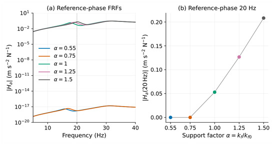
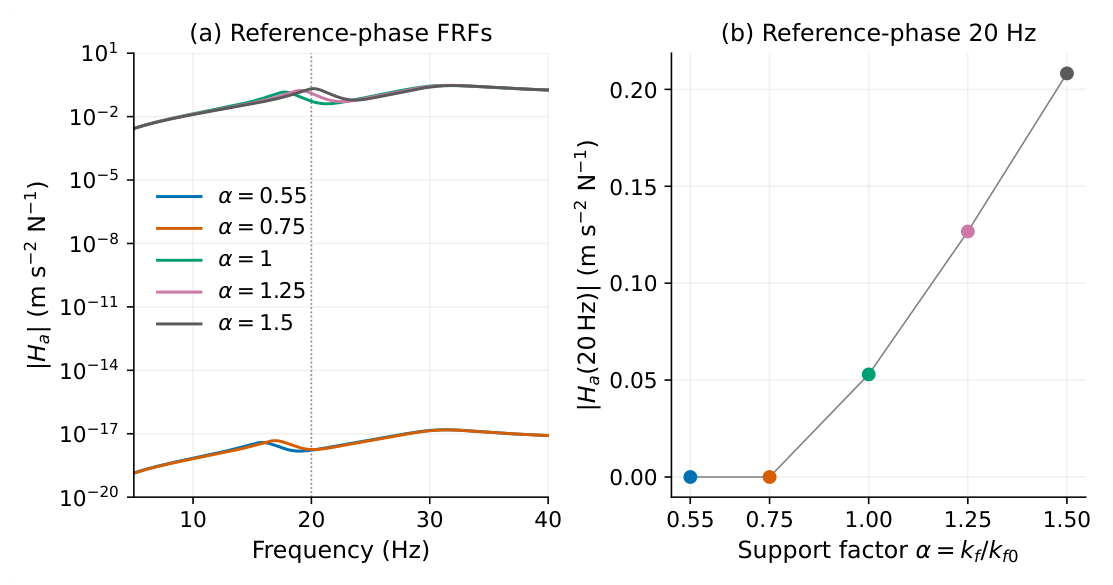
Figure 2 retains the frozen FRF results. The 20 Hz values at $\alpha =0.55$ and 0.75 are approximately $1.66\times {10}^{-18}$ and $1.79\times {10}^{-18}$ m s⁻² N⁻¹. At $\alpha =1$, 1.25, and 1.5 they are 0.05294, 0.12668, and 0.20826 m s⁻² N⁻¹. At the two near-zero paths, automated local-extremum detection operates on roundoff-scale response; the returned peak/trough frequencies are not reported as physical resonances or antiresonances. At the other three factors, the sampled FRF maxima nearest 20 Hz occur at 17.72, 19.08, and 20.18 Hz, with corresponding minima at 21.32, 22.56, and 23.70 Hz. These are forced-response extrema of a stationary tangent model, not independently measured modes.

Figure 2. Archived stationary FRFs and 20 Hz transfer magnitudes. The two roundoff-scale paths do not support a physical interpretation of detected local extrema. New non-equivalent cage-phase checks are listed separately in Table 2.

The earlier phase check used $0^{\circ }$, ${45}^{\circ }$, ${90}^{\circ }$, and ${135}^{\circ }$. For eight identical, equally spaced rolling elements, these phases merely permute the same configuration. Its reported CV of zero therefore cannot establish configuration insensitivity. An additional, separate diagnostic evaluates $0^{\circ }$, ${11.25}^{\circ }$, ${22.55}^{\circ }$, and ${33.75}^{\circ }$ over one ${45}^{\circ }$ period. Equilibrium residuals satisfy the same ${10}^{-3}$ N criterion; a scaled least-squares refinement is explicitly recorded when Nelder–Mead alone fails. Table 2 gives the resulting finite-configuration statistics. At $\alpha =0.55$, the ${22.5}^{\circ }$ value is 0.0328422 m s⁻² N⁻¹, showing that the near-zero path is configuration specific. These four points are a sensitivity check, not a converged phase average or an operating nonlinear FRF.

Table 2. New non-equivalent configuration diagnostic. Mean and sample SD of four stationary transfer magnitudes; units m s⁻² N⁻¹. CV is dimensionless. These are not converged phase averages.

$\mathit{\alpha }$	Mean $|{\mathit{H}}_{\mathit{a}}\left(20\right)|$	Sample SD	CV
0.55	0.024501	0.016335	0.6667
0.75	0.026068	0.017380	0.6667
1.00	0.055756	0.001960	0.0351
1.25	0.125404	0.002262	0.0180
1.50	0.213323	0.004362	0.0205

3.5. Fixed 20 Hz Response and Sensitivity Within the Scan

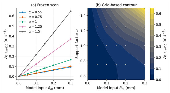
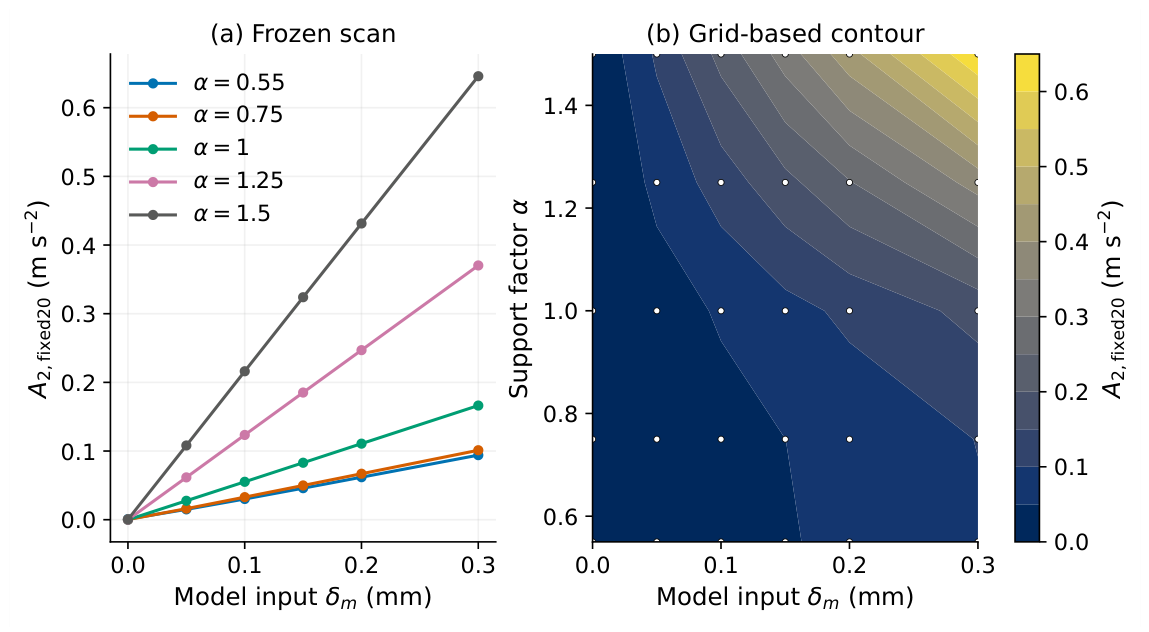
Table 3 gives the unchanged 30-case response matrix. At every fixed $\alpha$, the response increases with the model input setting; Spearman $\rho =1$. All nonzero-input band maxima occur at 20 Hz. The model therefore supplies support-dependent gain and input-setting sensitivity, not the observed experimental non-monotonic morphology. Figure 3 shows the curves and contour.

Table 3. Frozen-model $A_{2\mathrm{X}}\left(20\mathrm{Hz}\right)$ matrix (m s⁻²).

$\mathit{\alpha }={\mathit{k}}_{\mathit{f}}/{\mathit{k}}_{\mathit{f}0}$/${\mathit{\delta }}_{\mathit{m}}$ (mm)	0	0.05	0.10	0.15	0.20	0.30
0.55	0.000976	0.015077	0.030231	0.045949	0.061923	0.094069
0.75	0.000205	0.016168	0.032910	0.049901	0.066987	0.101215
1.00	0.000025	0.027602	0.055258	0.083016	0.110815	0.166299
1.25	0.000107	0.061685	0.123471	0.185248	0.246967	0.370318
1.50	0.000417	0.108140	0.216211	0.324030	0.431464	0.645907

Figure 3. Unchanged frozen-model fixed 20 Hz responses: (a) response to the equivalent-forcing input parameter ${\delta }_m$ at fixed support factor; (b) contour interpolated only between the 30 evaluated grid points.

For comparability of endpoint summaries, define

$$S\left(\alpha \right)={\displaystyle \frac{A_2({\delta }_m=0.30\mathrm{mm},\alpha )-A_2({\delta }_m=0.05\mathrm{mm},\alpha )}{0.25\mathrm{mm}}}.$$

(13)

Within the predefined 20 Hz scan, $S\left(0.55\right)=0.31597$ and $S\left(1.50\right)=2.15107$ m s⁻² mm⁻¹, a factor of 6.81. Relative to $\alpha =1$, these sensitivities are 0.569 and 3.877. Across the five scanned support states at a fixed nonzero input setting, the maximum amplitude ratio is 7.17. These factors apply only to this parameterization and scan interval; they are not material constants or experimental calibrations.

The endpoint sensitivities and reference-phase FRF values are summarized in Table 4.

Table 4. Sensitivity to the model equivalent-forcing input ${\delta }_m$ and reference-phase FRF of the frozen model. $\alpha =k_f/k_{f0}$; units of S are m s⁻² mm⁻¹ and units of $H_a$ are m s⁻² N⁻¹.

$\mathit{\alpha }$	S	$\mathit{S}/\mathit{S}\left(1\right)$	$|{\mathit{H}}_{\mathit{a}}\left(20\mathbf{Hz}\right)|$
0.55	0.31597	0.569	$1.66\times {10}^{-18}$
0.75	0.34019	0.613	$1.79\times {10}^{-18}$
1.00	0.55479	1.000	0.05294
1.25	1.23453	2.225	0.12668
1.50	2.15107	3.877	0.20826

3.6. Interpretation Boundary

The reference-phase $|H_a\left(20\mathrm{Hz}\right)|$ and $S\left(\alpha \right)$ have a descriptive Pearson association of $r=0.988$ over five support states. This association is configuration dependent and is not a proportionality law. The nonlinear results are obtained with rotating, changing contact, whereas the FRF is a local stationary linearization. The newly recovered phase sensitivity reinforces this distinction. At ${\delta }_m=0$ the misalignment force vanishes, but a fixed 20 Hz output and a weak band maximum need not vanish. The three-dimensional scan is shown in Supplementary Figure S1 (bottom panel). None of these calculations maps a physical experimental session to a specific support factor.

4. Experimental Records and Descriptive Cross-Session Results

4.1. Study Sessions and Operating Conditions

S4–S6 are the three independent normal-bearing reassembly sessions analyzed in this paper. Each contains six prescribed motor-base displacement settings, $\delta =0$, 0.05, 0.10, 0.15, 0.20, and 0.30 mm, and three within-session repeated acquisitions at each setting. There are 54 waveforms, not 54 independent reassembly samples. The common recorded labels are N (normal bearing), 600 r/min, 2.79 V load-control command, and ch2. Load voltage is a command label, not a calibrated torque measurement. Each waveform contains 589,824 samples. The median timestamp increment is 50 $\mathsf{\mu }$s, giving approximately 20,000 Hz, a timestamp span of 29.49115 s, and $N/f_s=29.4912$ s. Table 5 summarizes these conditions.

Table 5. Recorded conditions and replication structure. Command labels do not establish metrological accuracy.

Item	Recorded Value or Interpretation
Bearing state	N, normal-bearing label
Speed/load-control command	600 r/min/2.79 V
Motor-base settings $\delta$	0, 0.05, 0.10, 0.15, 0.20, 0.30 mm
Setting/verification	Adjustment screw/dial indicator at base center
Indicator range/graduation/label	0–10 mm/0.01 mm/004288
Displacement direction	Horizontal transverse motor-base displacement
Independent sessions	S4, S5, S6; three total
Acquisitions	Three per setting per session; 54 total
Channels/analysis	ch1 vertical; ch2 horizontal; ch2 analyzed
Acquisition hardware	DC-24 multifunction data acquisition unit
Sensor	VALENIAN 676067 ICP accelerometer
Sensor mounting	Magnetic attachment at bearing-housing positions; quantitative remounting/contact records unavailable
Nominal sensor sensitivity	100 mV/g at 25 ∘C, 160 Hz
Historical DC-24 setting	1.00000 mV/(m s−2), author confirmed for all 54 records
Derived experimental scale factor	$c_s=0.0980665$; not traceable calibration
Anti-aliasing	Internal automatic; not user-configurable
Exported unit	m s−2
Sampling/samples	Approximately 20,000 Hz/589,824
Record duration $N/f_s$	29.4912 s
Direct shaft-offset/angle record	Not found in the available archive
Instrument calibration/uncertainty	Not found in the available archive

S1–S3 were separate bearing experiments, not additional normal-bearing sessions belonging to the present study series. They are not pooled with S4–S6, treated as missing repetitions of the present protocol, or retrospectively designated as pilot sessions. The analysis population here is the three normal-bearing sessions S4–S6.

4.2. Displacement Setting and Measurement Chain

The quantity $\delta$ denotes a dial-indicator-verified motor-base displacement setting. The levels were imposed using the motor-base adjustment screw. At every level, a dial indicator rechecked horizontal transverse displacement at the central region of the motor base before three waveforms were acquired. The sequence was therefore adjustment screw, dial-indicator verification, and three waveform acquisitions. The zero setting denotes the session’s aligned operating reference, not certified zero residual shaft misalignment.

The dial indicator had a measurement range of 0–10 mm, a graduation of 0.01 mm, and equipment/label number 004288. It verified horizontal transverse displacement at the central region of the motor base at every setting before the three vibration records were acquired. The indicator verifies displacement of the motor base, not the offset between two shaft centerlines. No direct shaft-center-offset measurement, residual angular measurement, indicator calibration certificate, or quantified setting-uncertainty record was found in the available archive. Graduation must not be interpreted as measurement accuracy or a complete uncertainty estimate.

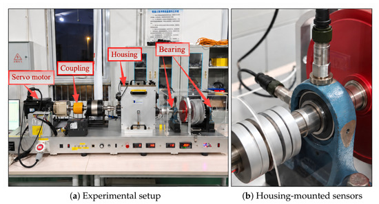
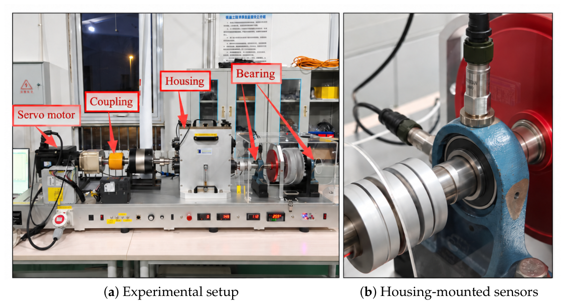
Figure 4 shows the rig and sensors at the test-side bearing housing. Channel ch1 is vertical and ch2 is horizontal; this paper analyzes ch2 only. The VALENIAN 676067 ICP (VALENIAN (Suzhou) Teaching Equipment Co., Ltd., Kunshan, China) piezoelectric accelerometers were magnetically mounted on the bearing housing at the vertical and horizontal measurement positions. The manufacturer specifications recovered by the authors give a nominal sensitivity of 100 mV/g at 25 °C and 160 Hz, a peak range of $\pm 50$ g, frequency responses of $\pm 10\%$ over 1–9000 Hz and $\pm 3$ dB over 0.4–12,000 Hz, and transverse sensitivity no greater than 5%. Exact remounting repeatability, magnetic-base seating consistency, contact condition, and session-specific mounting force or contact quality were not quantitatively recorded. No session-specific calibration certificate or traceable sensitivity calibration record is available.

Figure 4. Archived photographs of the rig and test-side bearing-housing sensors. The accelerometers were magnetically mounted; ch2 measures horizontal vibration and is analyzed here, whereas ch1 is vertical. Acquisition used the DC-24 unit. Exact remounting repeatability, magnetic-base seating consistency, contact condition, and session-specific mounting force or contact quality were not quantitatively recorded. The photograph alone does not establish channel wiring, calibration, or a quantitative transfer mapping.

Acquisition used a DC-24 multifunction data acquisition unit with internal automatic anti-aliasing. Its anti-aliasing parameters are not user-configurable in the acquisition interface. The filter cutoff, type, order, and transition bandwidth were not recovered and are not assumed. Sampling frequency and historical record length are verified from the archived time columns, rather than from later demonstration-screen settings.

The raw-file headers label the selected column 2-2[m s²]. The author confirmed that the historical acquisitions used a $1.00000$ mV/(m s⁻²) sensitivity setting, and no subsequent sensitivity correction was found in the recovered processing scripts. The manufacturer’s nominal SI-equivalent sensitivity is $S_{\mathrm{nom}}=100/9.80665\simeq 10.19716$ mV/(m s⁻²). Accordingly, this revision applies the same nominal-sensitivity correction to all experimental dimensional quantities:

$$a_{\mathrm{nom}}=c_s{a}_{\mathrm{export}},A_{\mathrm{nom}}=c_s{A}_{\mathrm{export}},c_s={\displaystyle \frac{S_{\mathrm{set}}}{S_{\mathrm{nom}}}}=0.0980665.$$

(14)

Here, $a_{\mathrm{export}}=V/S_{\mathrm{set}}$ describes the historical voltage-to-engineering-unit conversion; original voltage records were not recovered. The numerical conversion uses the unrounded ratio $100/9.80665$. Archived exports are preserved unchanged, and corrected outputs are stored separately with a value-by-value audit trail. Experimental amplitudes, means, SDs, slopes, baseline differences, and spectral-background amplitudes below use this nominal-sensitivity-corrected basis unless explicitly labeled as archived/exported. This is not a traceable calibration at 20 Hz: the sensitivity is specified at 160 Hz, the stated frequency-response tolerance remains, and no calibrated absolute acceleration accuracy or complete uncertainty budget is claimed. The correction does not apply to any model amplitude, FRF, force coefficient, or numerical diagnostic.

4.3. Reported Reassembly and Recording Boundary

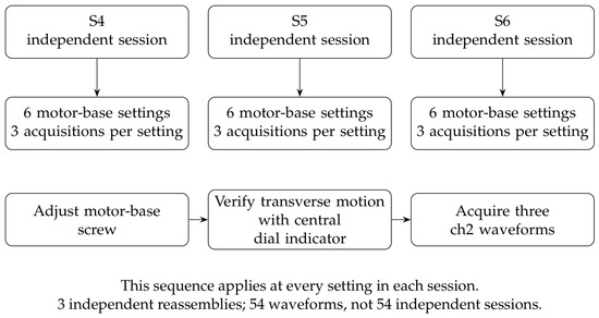
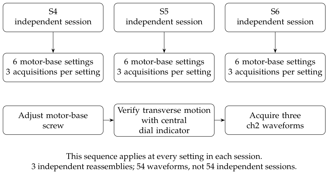
Normal independent reassembly and realignment preceded S4, S5, and S6, without deliberately creating soft or stiff states. The screw-adjustment and dial-indicator recheck sequence was applied at each of the six settings, followed by three acquisitions. Detailed numerical fastening torque, preload, and fit records were not found. The archived S6 setting and run templates have no completed required entries; they do not override the author-confirmed displacement-verification procedure. Magnetic attachment is known, but exact remounting repeatability, magnetic-base seating consistency, contact condition, session-specific mounting force or contact quality, and additional operator events were not quantitatively recorded. Figure 5 summarizes the confirmed sequence and replication structure.

Figure 5. Confirmed procedure and replication structure. Each setting follows screw adjustment, a central motor-base dial-indicator recheck of horizontal transverse displacement, and three acquisitions. Reassembly is the session-level factor; repeated waveforms are not independent reassemblies.

4.4. Recovered Signal-Processing Chain

The S5 and S6 scripts call the same analyze_waveform function defined in the S4 script. The nominally .xls inputs are tab-delimited text, not Excel workbooks. Column 0 contains time; numeric column 2 contains ch2. Every sample is used after checking finite values and increasing timestamps. No segment rejection, resampling, linear/polynomial detrending, or digital filtering is applied by this analysis code. The DC-24 automatic anti-aliasing is distinct from this post-export processing; its filter transfer function remains unavailable. The separate factor in Equation (14) changes the amplitude scale, not the original harmonic estimator.

For nominal-sensitivity-corrected samples $x_n=c_s{a}_{\mathrm{export},n}$, the mean is removed, $y_n=x_n-\overline{x}$, and a symmetric Hann window is applied:

$$w_n={\displaystyle \frac{1}{2}}\left[1-\cos {\displaystyle \frac{2\pi n}{N-1}}\right],X_k={\displaystyle \sum _{n=0}^{N-1}}{w}_n{y}_n\exp \left(-{\displaystyle \frac{2\pi \mathrm{i}kn}{N}}\right),f_k={\displaystyle \frac{k{f}_s}{N}}.$$

(15)

The one-sided amplitude spectrum is

$$A_k={\displaystyle \frac{2|X_k|}{{\sum }_n{w}_n}},1\le k<N/2.$$

(16)

DC and Nyquist are halved relative to this expression. Division by $\sum w_n=N{G}_c$ supplies coherent-gain correction. The reported quantity is a peak-amplitude-scaled spectral-bin amplitude, not RMS amplitude, power spectral density, or integrated band energy. The normalization is exact for a bin-centered sinusoid; off-bin leakage and scalloping remain possible because no interpolation or scalloping correction is applied.

The implemented frequency tracker selects the largest bin in 9.5–10.5 Hz:

$$k_1=\underset{k:9.5\le f_k\le 10.5}{\arg \max }{A}_k,f_{1\mathrm{X},measured}=f_{k_1},f_{2\mathrm{X}}=2f_{k_1},k_2=\underset{k}{\arg \min }|f_k-f_{2\mathrm{X}}|.$$

(17)

The retained code label “measured” denotes a vibration-spectrum estimate, not an independent tachometer measurement. $A_{1\mathrm{X}}=A_{k_1}$, $A_{2\mathrm{X}}=A_{k_2}$, and $R_{21}=A_{2\mathrm{X}}/A_{1\mathrm{X}}$. No frequency interpolation or narrow-band integration is used. An auxiliary peak is the largest amplitude within $2f_{k_1}\pm 0.5$ Hz; it is not substituted for the tracked primary metric. The bin width is approximately 0.0339084 Hz.

Across all 54 records, estimated $f_{1\mathrm{X}}$ ranges from 10.002984 to 10.036892 Hz, with mean 10.019310 Hz and sample SD 0.017102 Hz. The corresponding tracked 2X range is 20.005968–20.073785 Hz, mean 20.038620 Hz, and SD 0.034203 Hz, or 0.005968–0.073785 Hz above nominal 20 Hz. This narrow range motivates 20 Hz as a nominal model operating harmonic at 600 r/min; the record-specific experimental metric is nevertheless retained. Before the nominal-sensitivity correction, re-extraction reproduces all archived primary amplitudes to a maximum absolute difference of $8.33\times {10}^{-17}$ in the exported m s⁻² units. An all-record check verifies that scaling samples before the FFT gives the same spectrum, within floating-point tolerance, as scaling the archived spectral amplitudes afterward.

4.5. Sensitivity to the Harmonic Estimator

The archived auxiliary local peak permits a direct check of estimator dependence without changing the primary metric. In 41 of 54 records (18/18 for S4, 12/18 for S5, and 11/18 for S6), the local peak differs from the tracked target by one FFT bin, approximately 0.0339084 Hz. Peak-to-tracked amplitude ratios range from 1 to 2.08684. Selecting a quantized 1X bin and doubling its frequency does not guarantee selection of the strongest 2X bin; the Hann-window response and frequency quantization can materially affect the resulting amplitude.

Table 6 compares the two estimators’ endpoint slopes after nominal-sensitivity correction. In particular, the S5 slope changes from $+0.033157$ for the tracked bin to $-0.025183$ m s⁻² mm⁻¹ for the local peak. Thus the slope-sign contrast is not estimator independent. The local maximum is not assumed to be the true harmonic amplitude either: it may include nearby components and is a different estimator. Neither metric is substituted for the other or chosen to obtain a preferred shape. The records establish differences in the retained tracked-bin metric, but they do not isolate physical assembly effects from frequency-estimation and amplitude-extraction effects.

Table 6. Nominal-sensitivity-corrected endpoint slopes (m s⁻² mm⁻¹) for the archived estimators. The local peak is auxiliary, not ground truth or a replacement for the tracked primary metric.

Session	Tracked-Bin Slope	Local-Peak Slope	Different Peak Bin
S4	$-0.006291$	−0.013021	18/18
S5	+0.033157	−0.025183	12/18
S6	$-0.011725$	−0.043331	11/18

4.6. Local Spectral Background and 2X-to-Background Ratio

A common revision-stage rule assesses the local spectrum for every record. The eligible bins lie within $f_{2\mathrm{X}}\pm 3$ Hz. Bins within $\pm 0.20$ Hz of each integer order $h{f}_{1\mathrm{X}}$, $h=1,\dots ,5$, are excluded; within this local interval, only the 2X exclusion is active. The guard contains the target and its immediate window leakage neighborhood. No record-specific regions are selected. The estimator is the median amplitude of the remaining bins,

$$A_{\mathrm{bg}}={median}_{k\in \mathcal{B}}{A}_k,{\mathrm{SBR}}_{2\mathrm{X}}=20{\log }_{10}\left({\displaystyle \frac{A_{2\mathrm{X}}}{A_{\mathrm{bg}}}}\right).$$

(18)

This is a local spectral-background ratio, not an integrated broadband SNR or a calibrated instrument noise-floor measurement. Unknown sidebands and deterministic leakage are not silently classified as electronic noise. It cannot recover missing calibration or filter-transfer-function information. The common nominal-sensitivity factor scales both numerator and denominator, leaving this ratio unchanged, as verified record by record.

The minimum, median, and maximum ratios are 40.20, 44.97, and 49.98 dB, respectively. Session and condition summaries, along with uniform 0.10 and 0.30 Hz guard sensitivity checks, are supplied in the reproducibility package. Table 7 reports the session summaries, and Supplementary Figure S2 shows all 54 local spectra. These results indicate separation from the defined local background; they do not establish unbiased harmonic amplitudes or independence of repeats.

Table 7. Local 2X-to-background ratios for all retained records; a common $\pm 3$ Hz window and $\pm 0.20$ Hz order exclusion are used.

Session	Records	Minimum (dB)	Median (dB)	Maximum (dB)
S4	18	41.88	44.41	45.89
S5	18	40.20	45.60	49.98
S6	18	42.32	46.09	49.35

4.7. Statistics and Data Integrity

For each motor-base displacement setting, mean, sample SD ($n-1$ denominator), and CV are computed over three within-session repeated acquisitions. Cross-session CV uses the three session means. There were three independent reassembly sessions. Because only three were available, the cross-session analysis is descriptive and no population-level inference regarding assembly-to-assembly variability is intended. No record is treated as a separate reassembly realization.

The endpoint slope uses Equation (13), applied to each session-mean curve versus nominal setting. Local slopes are adjacent finite differences of those means. Their CV is sample SD divided by the absolute signed mean and can be large or unstable when positive and negative slopes cancel. Spearman and Pearson correlations summarize six means without establishing a calibrated severity law. All 54 records are retained; no non-monotonic point is removed or reassigned. Checks confirm finite samples, readable records, and increasing timestamps. Original integrity rules flag a timestamp increment departure above 10% or non-finite data; amplitude or curve shape alone is not an invalidity rule.

4.8. Within-Session Variation and Observed Mean Curves

Mean repeat CVs are 7.48%, 11.67%, and 13.62% for S4, S5, and S6; their maxima are 14.39%, 19.08%, and 33.84%. The largest is the S6 aligned reference, which remains in the analysis. Precision is not uniform across conditions. With only three acquisitions per setting, neither a low CV nor a visible change in a mean establishes a stable population property.

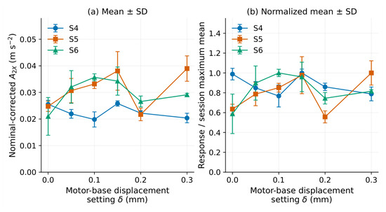
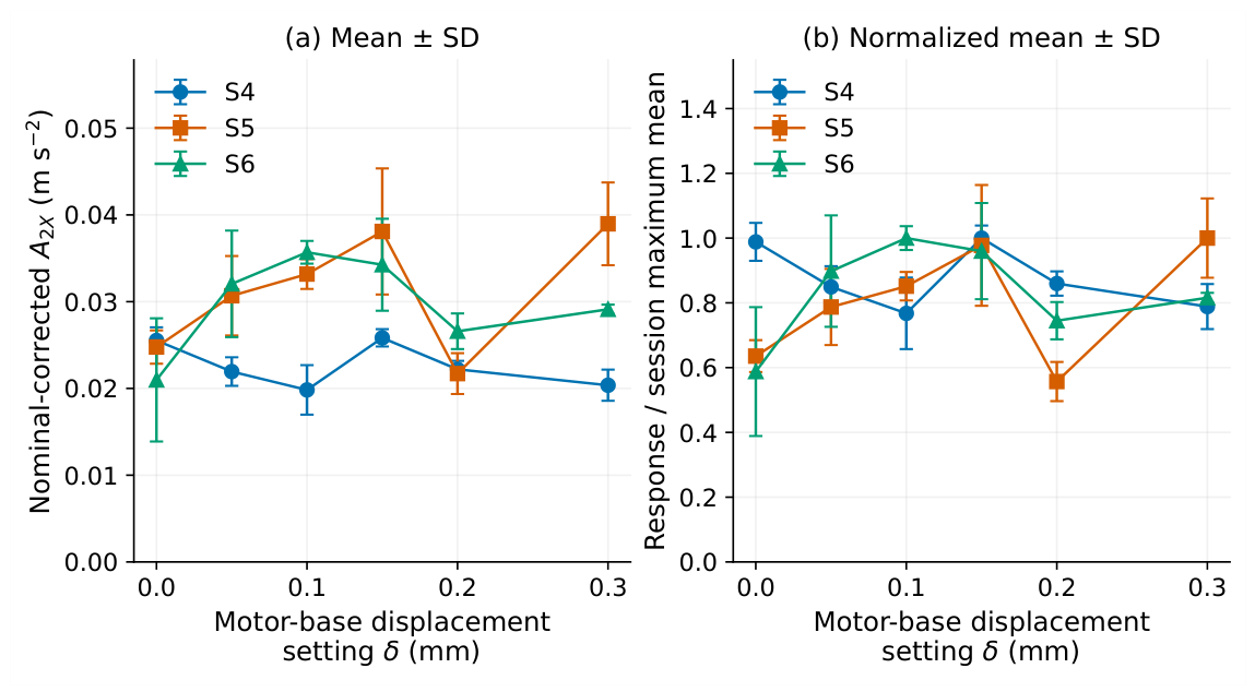
Table 8 and Figure 6 show the nominal-sensitivity-corrected means and sample SD. S4 decreases to 0.019830 m s⁻² at 0.10 mm, rises at 0.15 mm, and ends at 0.020370 m s⁻². S5 rises to 0.15 mm, falls to 0.021708 m s⁻² at 0.20 mm, and rises to 0.038971 m s⁻² at 0.30 mm. S6 reaches 0.035692 m s⁻² at 0.10 mm before decreasing and rising again. All three session-mean curves have observed direction changes.

Table 8. Nominal-sensitivity-corrected tracked $A_{2\mathrm{X}}$ means (m s⁻²). Archived exported values remain unchanged in the source records.

Session/$\mathit{\delta }$ (mm)	0	0.05	0.10	0.15	0.20	0.30
S4	0.025532	0.021943	0.019830	0.025832	0.022208	0.020370
S5	0.024770	0.030682	0.033181	0.038092	0.021708	0.038971
S6	0.020981	0.032052	0.035692	0.034256	0.026588	0.029120

Figure 6. Response versus dial-indicator-verified motor-base displacement setting for the three sessions: (a) nominal-sensitivity-corrected tracked 2X means with sample-SD bars over three acquisitions; (b) the same means and SD divided by each session’s maximum mean. Connecting lines guide the eye; no smoothing or fitted morphology is used.

The endpoint slopes are $-0.006291$, $+0.033157$, and $-0.011725$ m s⁻² mm⁻¹. Spearman coefficients are $-0.200$, $+0.429$, and $+0.0857$. The observed local-slope sign sequences are $-,-,+,-,-$, $+,+,+,-,+$, and $+,+,-,-,+$. These are descriptive properties of six means per session, not established repeatable morphology classes. Table 9 uses the corrected dimensional scale. Recalculation verifies that the common positive factor leaves CVs, cross/within CV ratios, max/min ratios, normalized curves, Spearman/Pearson coefficients, $R_{21}$, local-slope signs, and descriptive monotonicity classifications unchanged within floating-point tolerance.

Table 9. Session-curve statistics. Slopes use nominal-sensitivity-corrected m s⁻² mm⁻¹. All three tracked-bin curves remain descriptively non-monotonic. The last column is mean within-session repeat CV.

Session	$\mathit{\rho }$	r	Overall S	Mean Local S	Local-S CV	Repeat CV
S4	−0.200	−0.428	−0.006291	−0.016969	4.705	7.48%
S5	0.429	0.428	+0.033157	+0.022279	9.000	11.67%
S6	0.0857	0.183	−0.011725	+0.027493	4.998	13.62%

4.9. Fixed-Setting Cross-Session Comparison

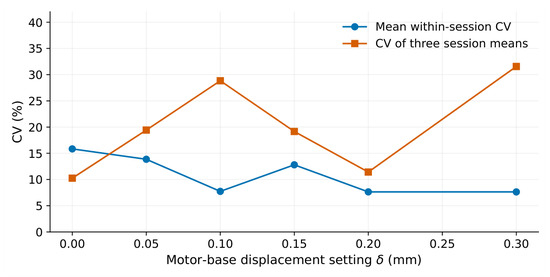
Cross-session CV ranges from 10.26% to 31.56%. At the aligned reference, the nominal-sensitivity-corrected session means are 0.025532, 0.024770, and 0.020981 m s⁻², showing that experimental 2X is not exclusively attributable to the nominally imposed setting. At 0.30 mm, the S5/S4 mean ratio is 1.913, the largest among the six nominal levels. At 0.10 and 0.30 mm, cross-session CV is 28.84% and 31.56%, compared with mean within-session CVs of 7.74% and 7.64%. The corresponding descriptive ratios are 3.72 and 4.13. They are not significance tests or variance-component estimates. At the aligned reference, within-session dispersion is larger, influenced by the S6 baseline. Table 10 summarizes these fixed-setting dispersions.

Table 10. Cross-session dispersion at a fixed motor-base displacement setting and comparison with within-session dispersion.

$\mathit{\delta }$ (mm)	Cross-Session CV	Mean Within-Session CV	Cross/Within	Max/Min	Note
0	10.26%	15.84%	0.65	1.217	Nonzero baseline 2X
0.05	19.43%	13.86%	1.40	1.461
0.10	28.84%	7.74%	3.72	1.800	Key difference
0.15	19.16%	12.81%	1.50	1.475
0.20	11.42%	7.64%	1.49	1.225
0.30	31.56%	7.64%	4.13	1.913	Largest difference

Figure 7 compares the two descriptive CV levels.

Figure 7. Descriptive dispersion: cross-session CV of three means and mean within-session CV of three acquisitions per setting. The two CVs describe different replication levels.

4.10. Normalized Shape, Local Slopes, and Auxiliary Ratio

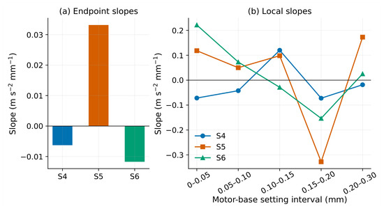
Normalization by a session-wise maximum does not remove the different locations of observed rises and decreases in the tracked-bin metric, including the S5 decline near 0.20 mm. Within this metric and these three sessions, the differences therefore are not represented fully by one constant amplitude scale. This does not establish an estimator-independent physical shape difference, a population-level morphology, or its cause. Figure 8 shows the observed local slopes of the session-mean curves.

Figure 8. Nominal-sensitivity-corrected endpoint and adjacent local slopes of the observed session means versus motor-base displacement setting. Mixed signs are retained, without inferring statistical significance or a stable population morphology.

The auxiliary $R_{21}$ comparison does not consistently reduce cross-session variability in these records (Supplementary Figure S1, top panel). Absolute tracked 2X remains the primary outcome. Subtracting the aligned-reference mean is shown separately in Supplementary Table S4; it does not change any finite-difference slope mathematically and is not independent evidence for slope robustness.

5. Model–Experiment Comparison and Evidence Boundary

The experimental outcome is $A_{2\mathrm{X}}=A\left(2f_{1\mathrm{X},measured}\right)$ at horizontal ch2, whereas the model reports housing x acceleration at fixed 20 Hz. The experimental frequency estimate is record-specific; its range is close to nominal 20 Hz but not identical to it. Both outputs represent a horizontal response direction conceptually. This does not establish a calibrated quantitative equivalence between the physical rig and the reduced model. The model has a directionally combined force input and a single-axis output; no support-independent ratio mapping its amplitude to measured ch2 has been established.

The model output is therefore not interpreted as a quantitative prediction of the measured ch2 amplitude. It is used only to test whether an equivalent support-state change can alter transfer gain and 2X sensitivity under a controlled harmonic input. Its ${\delta }_m$ parameter controls equivalent forcing; the experimental $\delta$ is a dial-indicator-verified horizontal motor-base displacement, not a direct shaft-center offset. The model parameter ${\delta }_m$ is neither a measured shaft-center offset nor a calibrated mapping from experimental $\delta$. The model’s 20 Hz forcing is exactly bin-centered, whereas the experimental tracker is quantized and its endpoint slopes are estimator dependent. These differences preclude pointwise amplitude fitting or attribution of a session to one support factor.

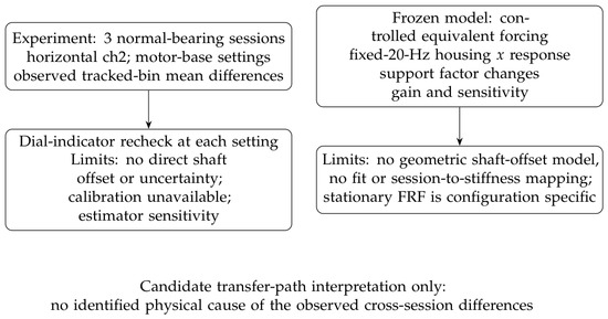
Within the predefined 20 Hz scan, all five response curves increase and their endpoint sensitivities differ. The experimental session-mean curves instead contain direction changes and slopes of different signs. The model establishes a possible gain mechanism within its parameterization, but does not reproduce those observed mean shapes. This mismatch is retained as an evidence boundary rather than removed by changing coefficients. Figure 9 separates observations from the candidate interpretation.

Figure 9. Evidence boundary. Observed session-mean differences and a model-specific support-gain mechanism are complementary findings, not a calibrated causal link. The diagram contains no fitted experimental stiffness or illustrative response curve.

Baseline subtraction supplies a limited additional description. It cannot change endpoint or local finite-difference slopes because it subtracts a session-wise constant. At nominal settings 0.10 and 0.30 mm, the ranges of baseline-subtracted means on the nominal-sensitivity-corrected scale are 0.020412 and 0.019362 m s⁻², respectively. The observed differences are therefore not represented solely by a constant reference offset. This check does not identify their source, remove measurement uncertainty, or replace the absolute response metric.

6. Discussion

6.1. What the Three Sessions Can Establish

The archive documents differences among three session-mean responses under nominally matched conditions. It does not estimate a population distribution of assembly-to-assembly variability. Three acquisitions per setting characterize within-session dispersion only; they do not increase the independent reassembly sample size beyond three. A sign change or peak in a six-point mean curve is consequently an observed feature, not proof of a reproducible morphology class. The retained within-session dispersion, especially the S6 reference CV, further limits strong shape comparisons.

The status of $\delta$ is central to interpretation. Every motor-base displacement setting was rechecked with a dial indicator of known range and graduation, so it would be incorrect to describe the setting procedure as unverified. Nevertheless, that procedure does not directly measure shaft-center offset or residual angle, and its uncertainty cannot be quantified from graduation alone without calibration and reading records. These geometric quantities cannot be separated from changes in structure or measurement conditions using the present records. Horizontal ch2 orientation, the VALENIAN 676067 sensor, magnetic attachment, the DC-24 unit, and its automatic anti-aliasing are known. The nominal-sensitivity correction resolves the confirmed common engineering-unit scale mismatch, not the missing traceable calibration or filter transfer function. The manufacturer’s sensitivity at 160 Hz and its frequency-response tolerance do not certify absolute acceleration accuracy at 20 Hz. Exact remounting repeatability, magnetic-base seating consistency, contact condition, and session-specific mounting force or contact quality were not quantitatively recorded. The S5 slope-sign change under the existing auxiliary local-peak estimator remains an additional substantive limitation: detailed slope signs and mean-curve shapes cannot be treated as estimator-independent physical responses. Strong 2X-to-background separation does not eliminate off-bin amplitude bias. Both archived estimators are retained rather than selecting the one that supports an assembly interpretation.

6.2. Candidate Transfer Mechanism, Not Causal Identification

The source–path–receiver framework is appropriate because a housing acceleration can vary through forcing, transmission, and sensing [10,11,12]. Support, pedestal, foundation, and housing models give mechanistic precedents for transfer changes [19,20,21,29]. Preload, fit, and assembly-related studies identify other possible influences [13,14,15,31]. None of these references documents a particular physical change in S4–S6.

Within the present parameterization, changing the support factor while holding the excitation law fixed is sufficient to change dynamic gain and input-setting sensitivity. The scan-specific factors of 6.81 for endpoint sensitivity and 7.17 for maximum fixed-setting response variation are not universal amplification factors. No model parameter was estimated from the experimental curves, and no experimental session was mapped to $k_f$. The result supports a candidate interpretation, not causal identification of support stiffness as the source of the observed cross-session differences.

6.3. Stationary Linearization and Configuration Dependence

The matched linear implementations agree, but agreement alone cannot identify a physical antiresonance. At the low-stiffness reference state, the contact tangent has essentially no horizontal transmission path. Finite contact motion and changing rolling-element position can produce a finite response in the nonlinear equations. The independent ablation supports this numerical possibility while preserving the frozen results.

The additional non-equivalent cage configurations also show why the original zero-CV phase check was insufficient. A single stationary FRF is local in both displacement and configuration. The four-point diagnostic is not a converged configuration average, a periodically time-varying transfer model, or a measured operating FRF. The descriptive association between reference-phase transfer and sensitivity must be interpreted with these limitations. At roundoff-scale paths, assigning physical resonance or antiresonance frequencies from automated extrema is unwarranted.

6.4. Experimental Non-Monotonicity and Model Boundary

The nonlinear model does not generate the direction changes observed in the three session-mean curves over the frozen grid. This is consistent with why a one-parameter transfer model may not reproduce a physical experiment involving unrecorded geometry, coupling forces, contact conditions, damping, and sensor-remounting variability. It does not demonstrate which omitted mechanism matters. Nonlinear coupling and bearing studies show that multiple mechanisms can affect harmonic response [2,3,4,27]. These possibilities are not fitted retrospectively to the current means. More parameters or a curve fit would not resolve the missing alignment metrology and session metadata.

6.5. Scope, Provenance, and Necessary Future Evidence

S1–S3 were separate bearing experiments and are not additional members or incomplete repetitions of this study’s normal-bearing series. S4–S6 are the three sessions analyzed here. Their 54 retained waveforms are readable and reproduce the archived exported amplitudes before the separately documented nominal-sensitivity correction, but three independent reassemblies remain insufficient for population-level generalization. The confirmed procedure, indicator graduation, sensor specification, and common historical sensitivity setting are distinguished from still-unavailable session-specific calibration, uncertainty and fastening records.

Future validation requires calibrated shaft-center and angular measurements in addition to the motor-base dial-indicator recheck, more independently reassembled sessions, documented fastening/preload and magnetic-sensor-remounting conditions, and measurement-chain calibration records. Local measured FRFs with known force and response axes would be needed to test a quantitative transfer mapping. Such evidence requires new measurements; it cannot be supplied by replotting existing data or tuning the frozen model. The present study is limited to a descriptive assessment and a bounded numerical mechanism test.

7. Conclusions

The three normal-bearing sessions had different mean 2X responses in the tracked spectral bins. Each horizontal motor-base displacement setting was verified with a dial indicator, and horizontal ch2 was acquired using the DC-24 unit. The retained endpoint slopes differed in sign and the six-point means contained local direction changes; however, the S5 slope becomes negative under the archived auxiliary local-peak estimator. These observations do not establish estimator-independent physical morphology, a population-level reproducibility property, or a calibrated relationship with directly measured shaft misalignment.

Within the predefined 20 Hz model scan, the support-state proxy was sufficient to change transfer gain and input-setting sensitivity while the equivalent 2X force remained proportional to the model input parameter ${\delta }_m$. The model curves remained increasing and did not reproduce the experimental mean morphologies. Matched linear frequency- and time-domain calculations agreed; additional contact and configuration checks limited the interpretation of the near-zero stationary FRF to its local linearization, rather than proving an isolated 20 Hz antiresonance.

No experimental session was assigned to a specific stiffness, and no physical assembly variable was causally identified. The confirmed setting verification does not supply direct shaft-offset/angle measurements or quantified uncertainty. A common nominal-sensitivity correction has been applied only to experimental dimensional quantities, preserving the archived exports and all model results. It does not supply a traceable 20 Hz calibration, session-specific certificates, or a complete uncertainty budget; the automatic anti-aliasing transfer function also remains unavailable. Absolute 2X amplitude should therefore not be treated as a transferable quantitative indicator without documenting these remaining conditions and checking harmonic-estimator sensitivity. Calibrated alignment measurements, additional independent reassemblies, quantitatively recorded magnetic-sensor-remounting conditions, fastening/preload records, measured local FRFs, and independent validation are necessary next steps.

References

- Wang, P.; Xu, H.; Ma, H.; Yang, Y.; Han, Q.; Wen, B.; Li, X. Nonlinear response of rotor system with bearing dynamic misalignment. Mech. Based Des. Struct. Mach. 2024, 52, 2532–2553. [Google Scholar] [CrossRef] [Scilit]
- Zhang, C.; Wang, D.; Zhu, R.; Chen, W.; Yu, C. Dynamic modeling and analysis of the rotor-bearing-disc coupling system with misalignment. Int. J. Dyn. Control 2023, 11, 2021–2035. [Google Scholar] [CrossRef] [Scilit]
- Zhang, C.; Cao, P.; Zhu, R.; Chen, W.; Wang, D. Dynamic modeling and analysis of the spline joint-flexible coupling-rotor system with misalignment. J. Sound Vib. 2023, 554, 117696. [Google Scholar] [CrossRef] [Scilit]
- Jiang, Z.; Huang, X.; Sun, L.; Wang, Y.; Jiang, F. Dynamic modeling and spectrum modulation effect of multi-type bearing-supported rotor systems with combined misalignment faults. J. Sound Vib. 2025, 609, 119118. [Google Scholar] [CrossRef] [Scilit]
- Miao, X.; He, J.; Jiang, D.; Zhang, D.; Pennacchi, P.; Fei, Q. Research on nonlinear vibration of a dual-rotor system with combined misalignment of cylindrical roller bearing and coupling. Nonlinear Dyn. 2025, 113, 3147–3170. [Google Scholar] [CrossRef] [Scilit]
- Ma, X.; Li, Z.; Xiang, J.; Sun, X.; Chen, C.; Huang, F. Nonlinear vibration analysis of rotor-bearing system with insufficient interference and bearing tilt. Int. J. Mech. Sci. 2025, 287, 109966. [Google Scholar] [CrossRef] [Scilit]
- Lal, M. Misalignment modeling and characteristic parameters estimation of a misaligned rotor-bearing assembly: An experimental investigation. Proc. Inst. Mech. Eng. Part K J. -Multi-Body Dyn. 2025, 239, 62–77. [Google Scholar] [CrossRef] [Scilit]
- Wang, Z.; Li, G.; Zhou, X.; Zhang, H.; Lin, Z.; Jia, S. Dynamic analysis of deep groove ball bearing with localized defects and misalignment. J. Sound Vib. 2024, 568, 118071. [Google Scholar] [CrossRef] [Scilit]
- Wang, P.; Yang, Y.; Ma, H.; Xu, H.; Li, X.; Luo, Z.; Wen, B. Vibration characteristics of rotor-bearing system with angular misalignment and cage fracture: Simulation and experiment. Mech. Syst. Signal Process. 2023, 182, 109545. [Google Scholar] [CrossRef] [Scilit]
- De Sitter, G.; Devriendt, C.; Guillaume, P.; Pruyt, E. Operational transfer path analysis. Mech. Syst. Signal Process. 2010, 24, 416–431. [Google Scholar] [CrossRef] [Scilit]
- Schünemann, W.; Schelenz, R.; Jacobs, G.; Vocaet, W. Identification of relevant acoustic transfer paths for WT drivetrains with an operational transfer path analysis. Forsch. Im. Ingenieurwesen 2021, 85, 345–351. [Google Scholar] [CrossRef] [Scilit]
- Tu, W.; Yang, J.; Luo, Y.; Jiang, L.; Xu, J.; Yu, W. Vibration Transmission Characteristics and Measuring Points Analysis of Bearing Housing System. Shock Vib. 2022, 2022, 4334398. [Google Scholar] [CrossRef] [Scilit]
- Gunduz, A.; Dreyer, J.T.; Singh, R. Effect of bearing preloads on the modal characteristics of a shaft-bearing assembly: Experiments on double row angular contact ball bearings. Mech. Syst. Signal Process. 2012, 31, 176–195. [Google Scholar] [CrossRef] [Scilit]
- Bal, H.; Ateş, K.; Karaçay, T.; Aktürk, N. Effect of Preload on the Vibrations of EHL Angular Contact Ball Bearings: Theoretical and Experimental Results. Lubricants 2022, 10, 46. [Google Scholar] [CrossRef] [Scilit]
- Wang, F.; Ling, X.; Zhang, Z.; Dai, P.; Yan, S.; Wang, L. The Effect of Fit Clearance between Outer Race and Housing on Vibration Characteristics of a Cylindrical Roller Bearing with Localized Defects. Machines 2022, 10, 415. [Google Scholar] [CrossRef] [Scilit]
- Cao, H.; Shi, F.; Li, Y.; Li, B.; Chen, X. Vibration and stability analysis of rotor-bearing-pedestal system due to clearance fit. Mech. Syst. Signal Process. 2019, 133, 106275. [Google Scholar] [CrossRef] [Scilit]
- Liu, P.; Wang, L.; Ma, F.; Zheng, D.; Wu, J.; Li, Z. Influence of assembly clearance on vibration characteristics of angular contact ball bearings in the thermal environment. Tribol. Int. 2023, 181, 108317. [Google Scholar] [CrossRef] [Scilit]
- Laine, S.; Haikonen, S.; Tiainen, T.; Viitala, R. Rotor resonance avoidance by continuous adjustment of support stiffness. Int. J. Mech. Sci. 2024, 270, 109092. [Google Scholar] [CrossRef] [Scilit]
- Yang, S.; Hu, Y.; Xiao, Z.; Zhang, C.; Tai, X. Rotor Vibration Analysis of Large-scale Centrifugal Compressor under the Flexible Support. J. Mech. Eng. 2019, 55, 121–127. [Google Scholar] [CrossRef] [Scilit][Green Version]
- Liu, J. A stiffness optimization method for a shaft-bearing-pedestal system based on the dynamics. Proc. Inst. Mech. Eng. Part K J.-Multi-Body Dyn. 2021, 235, 235–245. [Google Scholar] [CrossRef] [Scilit]
- Yang, D.Y.; Huang, J.L.; Zhu, W.D. Investigation on vibration characteristics of a rotor system with combined misalignment and eccentric faults under foundation swinging motion: Theoretical and experimental analyses. Mech. Syst. Signal Process. 2025, 240, 113332. [Google Scholar] [CrossRef] [Scilit]
- Guan, H.; Ma, H.; Chen, X.; Mu, Q.; Zeng, Y.; Chen, Y.; Wen, B.; Guo, X. Nonlinear vibration of rotor-bearing system considering base-motion and bearing-misalignment. Mech. Mach. Theory 2025, 206, 105933. [Google Scholar] [CrossRef] [Scilit]
- Zmarzły, P.; Wrzochal, M.; Adamczak, S. Evaluation of the Variability of Vibration Measurement Results in Rolling Bearing Quality Control. Appl. Sci. 2025, 15, 904. [Google Scholar] [CrossRef] [Scilit]
- Chen, H.; Lin, J.; Zhao, W.; Shu, H.; Xu, G. Evaluating Measurement System Capability in Condition Monitoring: Framework and Illustration Using Gage Repeatability and Reproducibility. Struct. Control Health Monit. 2025, 2025, 3441846. [Google Scholar] [CrossRef] [Scilit]
- Juzek, M.; Słowiński, P. The impact of accelerometer mounting on the correctness of the results obtained in NDT-type tests. Transp. Probl. 2024, 19, 97–105. [Google Scholar] [CrossRef] [Scilit]
- Kim, J.M.; Kim, H.H.; Nam, T.K. Leakage-Free, Cross-Speed, and Cross-Session Evaluation of Vibration-Based Propulsion-Shaft Misalignment Diagnosis in Electric Ships: A Real-Time Detect-Then-Grade Cascade. J. Mar. Sci. Eng. 2026, 14, 1464. [Google Scholar] [CrossRef] [Scilit]
- Li, B.; Li, Z.; He, D. Nonlinear dynamic analysis of rolling element bearings with misalignment defects. Int. J. Non-Linear Mech. 2026, 181, 105286. [Google Scholar] [CrossRef] [Scilit]
- Sun, X.; Chocholaty, B.; Liu, Y.; Marburg, S. Nonlinear dynamic behavior of a rotor-bearing system considering time-varying misalignment. Int. J. Mech. Sci. 2024, 284, 109772. [Google Scholar] [CrossRef] [Scilit]
- Cao, L.; Brouwer, M.D.; Sadeghi, F.; Stacke, L.E. Effect of Housing Support on Bearing Dynamics. J. Tribol. 2016, 138, 011105. [Google Scholar] [CrossRef] [Scilit]
- Shafiee, A.; Sadeghi, F.; Wilmer, M.G. An Integrated Finite Element and ADAMS Modeling Approach for Analyzing Rotor-Bearing Housing Systems. J. Tribol. 2025, 147, 014303. [Google Scholar] [CrossRef] [Scilit]
- Guan, H.; Wang, P.; Xiong, Q.; Ma, H.; Zhou, S.; Mu, Q.; Zeng, Y.; Chen, Y. Modeling of misaligned bearing induced by coupling misalignment and assembly errors and vibration analysis in dual-rotor system. Mech. Syst. Signal Process. 2025, 230, 112656. [Google Scholar] [CrossRef] [Scilit]
Disclaimer/Publisher’s Note: The statements, opinions and data contained in all publications are solely those of the individual author(s) and contributor(s) and not of MDPI and/or the editor(s). MDPI and/or the editor(s) disclaim responsibility for any injury to people or property resulting from any ideas, methods, instructions or products referred to in the content. |
© 2026 by the authors. Licensee MDPI, Basel, Switzerland. This article is an open access article distributed under the terms and conditions of the Creative Commons Attribution (CC BY) license.