Multi-Agent Reinforcement Learning for Dynamic Parallel-Machine Scheduling with Human–Robot Collaboration and Worker Fatigue

Abstract

This study investigates a dynamic parallel-machine scheduling problem with human–robot collaboration (DPMS-HRC), where dynamically arriving jobs are assigned to eligible workstations and processed by workers, robots, or human–robot collaboration based on real-time system states. Worker-involving modes improve operational flexibility but may increase actual processing times and cause uneven fatigue distribution due to fatigue accumulation. To coordinate production responsiveness and fatigue management, a weighted objective combining average flow time and the worker fatigue balance index is minimised. A mixed-integer nonlinear programming (MINLP) formulation is developed to model dynamic job arrivals, alternative processing modes, worker–robot allocation, and fatigue-dependent processing times. An action-masked and potential-shaped multi-agent proximal policy optimisation (AMPS-MAPPO) algorithm is then designed. Action masking restricts policy sampling to structurally feasible job-mode-resource combinations, while time-scaled potential shaping provides dense feedback for long-horizon learning. Experiments on dynamic instances of different scales show that AMPS-MAPPO achieves millisecond-level online inference, reduces average flow time by 40.98% relative to the best dispatching-rule benchmark and by 8.17–20.92% relative to deep reinforcement learning baselines, and obtains the lowest overall worker fatigue balance index among the compared deep reinforcement learning algorithms.

1. Introduction

Advances in intelligent manufacturing and the growing demand for personalised products are driving manufacturing systems away from conventional large-scale, rigid production towards small-batch, multi-variety, and flexible production [1]. Compared with mass production, such environments are characterised by heterogeneous order types, variable quantities, uncertain arrival times, and diverse processing requirements. These features give rise to dynamic scheduling problems, which differ fundamentally from their static counterparts. In static scheduling, jobs and resource requirements are usually known in advance, whereas in dynamic shop-floor environments, new jobs arrive during execution and resource states evolve over time. Pre-generated schedules may no longer match the current shop-floor state [2]. Dynamic scheduling requires online adjustment to continuously coordinate jobs and resources in response to real-time changes, while controlling unnecessary waiting and average flow time [3].

Human–robot collaboration (HRC) provides an important means of improving shop-floor flexibility in dynamic production environments [4,5]. Its flexibility comes from the complementarity between workers and robots: workers are suitable for judgement-based and complex operations, whereas robots provide stable performance in repetitive and high-intensity tasks [4,5]. HRC scheduling cannot be reduced to job sequencing, because worker, robot and human–robot collaborative processing modes differ in processing efficiency, resource occupation and coordination requirements [6]. The scheduling system must jointly determine job selection, workstation assignment, processing-mode selection, and worker–robot resource allocation [7].

One important distinction between human workers and robots is that worker fatigue changes with work and rest [8]. Continuous work causes fatigue accumulation, while idle or rest periods allow fatigue to recover [9]. Changes in fatigue make worker availability and processing efficiency state-dependent rather than fixed resource attributes [10]. A worker-involving assignment affects not only the current job but also the worker’s fatigue state, later processing times and subsequent resource assignment [8,9]. Therefore, focusing only on job-flow efficiency may lead to uneven fatigue distribution among workers. Coordinating production responsiveness and fatigue management, measured by average flow time and the worker fatigue balance index, is a key challenge in dynamic HRC scheduling.

The parallel-workstation setting is considered because each single-operation job can be processed on one of several eligible workstations, while workers and robots are shared across workstations and allocated dynamically according to the current system state. Accordingly, the aim of this study is to develop an online scheduling framework for the DPMS-HRC problem that coordinates job-flow efficiency and worker fatigue balance under dynamic job arrivals, fatigue-dependent processing times, and shared human–robot resources. To this end, average flow time and the worker fatigue balance index are combined through a weighted-sum objective, and a mixed-integer nonlinear programming (MINLP) formulation together with an action-masked and potential-shaped multi-agent proximal policy optimisation (AMPS-MAPPO) algorithm is developed.

The study contributes to dynamic HRC scheduling in three respects. It formulates the interaction among dynamic job arrivals, fatigue-dependent processing times, three processing modes, and shared human–robot resources in a parallel-workstation environment. It also develops an event-driven multi-agent scheduling framework in which workstation decisions are coordinated through sequential micro-steps over shared resources. Finally, the computational study examines the scheduling performance of the proposed approach across different problem scales, arrival conditions, resource configurations, and  algorithmic settings.

The remainder of this study is organised as follows. Section 2 reviews the related literature. Section 3 describes the DPMS-HRC problem and presents its MINLP formulation. Section 4 presents the AMPS-MAPPO algorithm for solving the problem. Section 5 reports the numerical experiments and results. Section 6 discusses the main findings, managerial implications, and limitations, while Section 7 concludes the study.

2. Literature Review

The related literature is reviewed along three streams: human–robot collaborative scheduling, human factors in production scheduling, and deep-reinforcement-learning-based scheduling.

2.1. Human–Robot Collaborative Scheduling

For HRC assembly-line balancing and scheduling, Nourmohammadi et al. [11] considered straight and U-shaped layouts and developed a mixed-integer linear programming model to optimise station configuration, cycle time and energy cost. Zheng et al. [12] studied HRC assembly lines with heterogeneous collaborative robots and limited resources. They proposed a constraint programming model and an improved fruit fly optimisation algorithm to optimise cycle time under human–robot parallel operations.

Beyond assembly lines, Inkulu and Bahubalendruni [13] investigated human–robot task allocation and estimated the allocation ratio between human and robotic resources to reduce total idle time. Huang et al. [14] addressed fixed-type multi-robot collaborative scheduling in flexible job shops. They decomposed the problem into flexible job-shop scheduling with controllable processing times and multi-robot task balancing, and proposed a hybrid GA-CP method. Zhang and Fujimura [15] studied HRC assembly lines with shared workstations. They used an enhanced simulated annealing algorithm with a task reassignment heuristic to reduce workload imbalance, cycle time and the number of operators. More recently, Wu et al. [16] studied dynamic HRC flexible job-shop scheduling under safety-proximity disruptions and developed a multi-agent reinforcement learning approach considering carbon emissions and human workload imbalance.

2.2. Human Factors in Production Scheduling

Early studies considered how learning and fatigue affect processing performance in scheduling. Dondeti and Mohanty [17] incorporated learning and fatigue into single-machine scheduling by treating processing time as a workload-dependent variable, while Biskup [18] analysed position-dependent learning effects. Later studies incorporated fatigue and recovery into multi-resource scheduling. Berti et al. [19] considered rest allowance and human energy expenditure in dual-resource job-shop scheduling and designed a task-assignment heuristic to balance production performance and worker well-being. Tan et al. [20] addressed a flexible job-shop scheduling problem and minimised makespan and maximum worker fatigue using an enhanced NSGA-II algorithm. Song et al. [21] considered real-time productivity changes in a distributed hybrid flow shop and used a Q-learning-driven multi-objective evolutionary algorithm to optimise makespan and energy consumption.

Other studies have extended human-factor modelling from fatigue to cognition, emotion, behavioural uncertainty and individual differences. Tropschuh et al. [22] reviewed physiological and psychological factors in employee scheduling. Zhang and Fujimura [23] considered cycle time, cognitive load balance and ergonomic risk in HRC assembly lines. Shi et al. [24] described boredom caused by repetitive tasks through an efficiency degradation function. Djogdom et al. [25] and Bouaziz et al. [26] examined the influence of operator execution deviations and punctuality uncertainty on collaboration fluency and system throughput. Herrmann et al. [27] focused on workers’ task-sequencing autonomy and incorporated individual sequencing preferences into flexible job-shop scheduling through a learning-to-rank method.

Human factors have also been integrated into HRC scheduling [28]. You et al. [29] studied HRC assembly task planning under uncertainty in physical exertion and execution time, and used reinforcement learning to learn adaptive task allocation policies. Park et al. [30] developed a scheduling model for HRC assembly workstations by considering ergonomic fatigue and simultaneous cooperation constraints. Hill and Vossen [31] analysed project scheduling with autonomous learning opportunities and examined how learning opportunities accelerate subsequent activities.

2.3. Deep Reinforcement Learning Scheduling

Studies on state representation and end-to-end decision architectures improve DRL scheduling policies by designing problem-specific representations of operations, machines, jobs and resources. Wang et al. [32] and Zhao et al. [33,34] enhanced feature representation for flexible job-shop scheduling through attention-based networks and heterogeneous disjunctive graph modelling, allowing operation–machine relations, random job arrivals and processing–transportation resource coordination to be captured in the decision process. Kim and Lee [35] combined deep reinforcement learning with a look-ahead search mechanism to improve robotic cell scheduling under uncertain processing times.

For dynamic disruptions, multi-objective optimisation and resource-related scheduling, DRL has been combined with local search, event-driven modelling and problem-specific policy design [36]. Panda et al. [37] formulated dynamic manufacturing resource matching as a sequential decision process and used DRL to learn resource-matching policies. Li et al. [38] and Yang et al. [39] incorporated problem-specific features into DQN-based scheduling methods. Rolim et al. [40] integrated Q-learning with simulated annealing for parallel-batch scheduling with setup times. Duan et al. [41] formulated event-driven predictive-reactive scheduling as a Markov jump decision process and solved it with a multi-objective hybrid deep Q-network. Ding et al. [42] incorporated human feedback into the reinforcement learning reward model to adapt scheduling policies to decision- maker preferences.

Multi-agent reinforcement learning has been used to coordinate decisions among multiple scheduling agents in distributed and collaborative production systems [43]. Zhang et al. [44] and Gu et al. [45] applied multi-agent learning to dynamic manufacturing scheduling. Zhang et al. [44] focused on cooperative job allocation and scheduling in distributed flexible job shops with dynamic disruptions and energy-efficiency requirements. Gu et al. [45] introduced large language models into MAPPO-based hybrid flow shop scheduling to enhance state representation and action selection.

2.4. Summary

Taken together, the literature shows that HRC scheduling has gradually moved from task allocation and assembly-line balancing towards the joint coordination of tasks and human–robot resources. In parallel, human-factor scheduling has incorporated fatigue, recovery, ergonomics, and other worker-related states into processing and assignment decisions, while DRL and multi-agent learning have increasingly been applied to dynamic scheduling with changing system states and coupled decisions. However, the reviewed studies address these aspects largely in separate settings, and their integration in dynamic HRC scheduling remains limited.

Recent studies have begun to extend HRC scheduling towards dynamic environments. Wu et al. [16], for example, considered safety-proximity disruptions in an HRC flexible job shop. However, dynamic job arrivals combined with fatigue-dependent processing times and shared human–robot resources in parallel-workstation environments remain insufficiently investigated. In such an environment, a scheduling decision at one workstation can affect both the immediate availability of shared workers and robots at other workstations and the subsequent processing efficiency of the assigned worker through fatigue evolution. Job selection, processing-mode selection, and human–robot resource allocation are therefore interdependent decisions rather than separate scheduling stages. The problem considered in this study captures these interactions under dynamic job arrivals and parallel-workstation processing.

Accordingly, a MINLP formulation is developed for the DPMS-HRC problem, together with an event-driven multi-agent scheduling framework for online decision-making. Workstations act as decision agents, while sequential micro-steps with temporary reservations of jobs, workers, and robots coordinate simultaneous decisions over shared resources. Action masking is used to maintain structural feasibility, and time-scaled potential shaping provides additional feedback during policy learning. Table 1 summarises the main characteristics of representative studies and the problem considered in this study.

Table 1. Comparison of related studies.

Literature	HRC	Fatigue	Dynamic	Objective	Method
Zheng et al. [12]	√	–	–	Cycle time	CP + FOA
Zhang and Fujimura [15]	√	–	–	Cycle time and operators	Enhanced SA
Dondeti and Mohanty [17]	–	√	–	Tardiness penalties	DP
Berti et al. [19]	–	√	–	Makespan and fatigue	Heuristic
Tan et al. [20]	–	√	–	Makespan and fatigue	Enhanced NSGA-II
Song et al. [21]	–	√	–	Makespan and energy	QMOEA
Park et al. [30]	√	√	–	Assembly makespan	AVNS
Zhao et al. [33]	–	–	√	Total tardiness	PPO-APN
Rolim et al. [40]	–	–	–	Total completion time	SA + Q-learning
Gu et al. [45]	–	–	√	Makespan	LLM-MAPPO
Wu et al. [16]	√	–	√	Makespan, carbon emissions, and human workload imbalance	CA-MADRL
This study	√	√	√	Average flow time and worker fatigue balance index	AMPS-MAPPO

3. Mathematical Formulation for the DPMS-HRC Problem

3.1. Problem Formulation

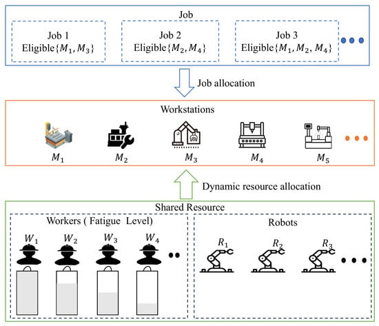
As shown in Figure 1, the studied DPMS-HRC problem is defined on a dynamic shop-floor environment. A set of single-operation jobs, denoted as $I=\{I_1,I_2,\dots ,I_n\}$, arrives dynamically over time. These jobs are processed on a set of parallel workstations, denoted as $M=\{M_1,M_2,\dots ,M_m\}$. Each job $I_i$ can be processed only on a job-specific subset of eligible workstations, denoted by $M_i\subseteq M$. The system is equipped with a shared multi-skilled resource pool consisting of workers $W=\{W_1,W_2,\dots ,W_w\}$ and robots $R=\{R_1,R_2,\dots ,R_r\}$. Both workers and robots can be allocated to different workstations according to the real-time system state. Worker fatigue is also considered, which accumulates during processing and recovers during idle periods. The scheduling horizon ends when all dynamically arriving jobs have been completed, and its end time is denoted by $T={\max }_{i\in I}{C}_i$.

Figure 1. Scheduling environment.

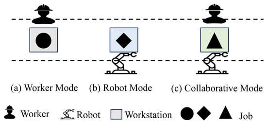
The baseline processing time of each job depends on the assigned workstation, whereas the actual processing time is further affected by the selected processing mode and, when a worker is involved, the worker fatigue state. As illustrated in Figure 2, each job can be processed under one of three processing modes. In the worker mode, one worker independently processes the job. In the robot mode, one robot independently processes the job. In the collaborative mode, one worker and one robot jointly process the job at the same workstation.

Figure 2. Three processing modes in the system.

To focus on the studied DPMS-HRC problem, the following assumptions are made (The assumptions are based on common settings in dynamic scheduling and HRC scheduling studies, including Poisson job arrivals, multi-skilled resources, and collaborative processing modes [46,47,48,49]).

(1)

Jobs arrive dynamically, and their arrival time follows a Poisson process.

(2)

Workers are assumed to be homogeneous in processing capability and share the same fatigue accumulation and recovery parameters, while robots are assumed to have identical processing capabilities.

(3)

Each worker or robot can process at most one job at a time.

(4)

All workers and robots are initially idle at time zero, and inter-workstation transfer times are neglected under the assumed compact shop-floor setting.

(5)

Each workstation can process at most one job at a time.

(6)

Once a job arrives, its eligible workstation set and baseline processing times are known and deterministic.

(7)

Once the processing of a job starts, it is non-preemptive and must continue until completion.

(8)

Each job must be assigned to exactly one eligible workstation and processed under exactly one processing mode.

A sequence-based formulation is adopted for the DPMS-HRC problem. Job assignments and resource conflicts are represented by assignment and sequencing variables, while immediate-successor variables are introduced for workers to link their processing sequences with fatigue recovery.

Table 2 summarises the parameters and decision variables used in the mixed-integer nonlinear programming (MINLP) formulation.

Table 2. Description of DPMS-HRC symbols.

Notation	Description
Sets
I	Set of jobs, indexed by $i,j$
M	Set of parallel workstations, indexed by m
$M_i$	Set of eligible workstations for job $I_i$
W	Set of workers, indexed by w
$W_0$	Extended set of workers, $W_0=W\cup \left\{w_0\right\}$, where $w_0$ is a virtual worker
R	Set of robots, indexed by r
$R_0$	Extended set of robots, $R_0=R\cup \left\{r_0\right\}$, where $r_0$ is a virtual robot
Parameters
$A_i$	Arrival time of job $I_i$
$d_i$	Due date of job $I_i$
$p{t}_{i,m}^{\mathrm{base}}$	Baseline processing time of job $I_i$ on workstation $M_m$
${\eta }_W,{\eta }_R,{\eta }_{\mathrm{Co}}$	Efficiency coefficients for worker, robot, and human–robot collaborative modes
${\lambda }_f$	Fatigue accumulation rate
${\mu }_f$	Fatigue recovery rate
$F^{\max }$	Operational fatigue threshold for new worker assignments
${\beta }_f^W,{\beta }_f^{\mathrm{Co}}$	Fatigue impact coefficients for worker and human–robot collaborative modes
$\omega$	Weight coefficient of the worker fatigue balance index
H	A sufficiently large positive constant
Binary decision variables
$x_{i,m,w,r}$	1 if job $I_i$ is assigned to workstation $M_m$ with worker resource $w\in W_0$ and robot resource $r\in R_0$, and 0 otherwise
${\delta }_{i,j}^m$	1 if job $I_i$ is processed before job $I_j$ on workstation $M_m$, and 0 otherwise, for $i<j$
$y_{w,i}$	1 if worker w is assigned to job $I_i$, and 0 otherwise
$q_w$	1 if worker w is used by at least one job in the schedule, and 0 otherwise
$a_{w,i}$	1 if job $I_i$ is the first job processed by worker w, and 0 otherwise
$b_{w,i}$	1 if job $I_i$ is the last job processed by worker w, and 0 otherwise
${\gamma }_{i,j}^w$	1 if job $I_j$ is processed immediately after job $I_i$ by worker w, and 0 otherwise, for $i\ne j$
${\zeta }_{i,j}^r$	1 if job $I_i$ is processed before job $I_j$ by robot r, and 0 otherwise, for $i<j$
Continuous variables
$S_i$	Start time of job $I_i$
$C_i$	Completion time of job $I_i$
T	End of the scheduling horizon, defined exactly as $T={\max }_{i\in I}{C}_i$
$P{T}_i$	Actual processing time of job $I_i$
$F_{w,i}^S$	Fatigue level of worker w at the start of job $I_i$
$F_{w,i}^C$	Fatigue level of worker w at the completion of job $I_i$
$F_w^{\mathrm{end}}$	Fatigue level of worker w at the end of the scheduling horizon
$\overline{F^{\mathrm{end}}}$	Average final fatigue level of all workers

Based on the above definitions, the optimisation objective is formulated as follows. The objective function in Equation (1) jointly considers production responsiveness and worker fatigue balance. The average flow time in Equation (2) measures the average time that dynamically arriving jobs spend in the system from arrival to completion. The worker fatigue balance index in Equation (3) measures the dispersion of workers’ fatigue levels at the end of the scheduling horizon and is used to evaluate the balance of residual worker fatigue. The two objectives are combined through a weighted-sum scalarisation, where $\omega$ controls the relative emphasis placed on fatigue balance.

$$\min F=f_1+\omega f_2$$

(1)

$$f_1={\displaystyle \frac{1}{\left|I\right|}}\sum _{i\in I}(C_i-A_i)$$

(2)

$$\begin{array}{cc}\hfill f_2& =\sqrt{{\displaystyle \frac{1}{\left|W\right|}}{\sum }_{w\in W}{\left(F_w^{\mathrm{end}}-\overline{F^{\mathrm{end}}}\right)}^2},\hfill \\ \hfill \overline{F^{\mathrm{end}}}& ={\displaystyle \frac{1}{\left|W\right|}}\sum _{w\in W}{F}_w^{\mathrm{end}}.\hfill \end{array}$$

(3)

Because the formulation contains nonlinear fatigue-dependent relationships and the worker fatigue balance objective, the resulting model is treated as a MINLP. In the Gurobi implementation, logarithmic and exponential terms are represented using general function constraints, while the fatigue-recovery product and fatigue-balance relationship are retained as nonconvex bilinear and quadratic constraints. Assignment and sequencing activation relationships are handled using Big-M and indicator constraints; no manual MILP linearisation of these nonlinear relationships is introduced. The constraints of the MINLP formulation are given as follows:

$$\begin{array}{ccccc}\hfill S_i& \ge A_i,\hfill & \hfill C_i& =S_i+P{T}_i,\hfill & \forall i\in I,\hfill \\ \hfill T& =\underset{i\in I}{\max }{C}_i.\hfill & \hfill & & \hfill \end{array}$$

(4)

$$P{T}_i=\sum _{m\in M_i}\sum _{w\in W_0}\sum _{r\in R_0}{x}_{i,m,w,r}{\widetilde{PT}}_{i,m,w,r},\forall i\in I.$$

(5)

$$\begin{array}{cccc}\hfill \sum _{m\in M_i}\sum _{w\in W_0}\sum _{r\in R_0}{x}_{i,m,w,r}& =1,\hfill & \hfill & \forall i\in I,\hfill \\ \hfill \sum _{m\in M_i}{x}_{i,m,w_0,r_0}& =0,\hfill & \hfill & \forall i\in I.\hfill \end{array}$$

(6)

$$\begin{array}{cc}\hfill S_j& \ge C_i-H(1-{\delta }_{i,j}^m)-H\left(2-\sum _{w\in W_0}\sum _{r\in R_0}{x}_{i,m,w,r}-\sum _{w\in W_0}\sum _{r\in R_0}{x}_{j,m,w,r}\right),\hfill \\ \hfill S_i& \ge C_j-H{\delta }_{i,j}^m-H\left(2-\sum _{w\in W_0}\sum _{r\in R_0}{x}_{i,m,w,r}-\sum _{w\in W_0}\sum _{r\in R_0}{x}_{j,m,w,r}\right),\hfill \end{array}\begin{array}{c}\forall i,j\in I,i<j,\\ m\in M_i\cap M_j.\end{array}$$

(7)

$$\begin{array}{cccc}\hfill y_{w,i}& =\sum _{m\in M_i}\sum _{r\in R_0}{x}_{i,m,w,r},\hfill & \hfill & \forall w\in W,i\in I,\hfill \\ \hfill y_{w,i}& \le q_w,\hfill & \hfill & \forall w\in W,i\in I,\hfill \\ \hfill q_w& \le \sum _{i\in I}{y}_{w,i},\hfill & \hfill & \forall w\in W.\hfill \end{array}$$

(8)

$$\begin{array}{cccccc}\hfill \sum _{i\in I}{a}_{w,i}& =q_w,\hfill & \hfill \sum _{i\in I}{b}_{w,i}& =q_w,\hfill & \hfill & \forall w\in W,\hfill \\ \hfill a_{w,i}+\sum _{j\in I:j\ne i}{\gamma }_{j,i}^w& =y_{w,i},\hfill & \hfill b_{w,i}+\sum _{j\in I:j\ne i}{\gamma }_{i,j}^w& =y_{w,i},\hfill & \hfill & \forall w\in W,i\in I.\hfill \end{array}$$

(9)

$$S_j\ge C_i-H(1-{\gamma }_{i,j}^w),\forall w\in W,i,j\in I,i\ne j.$$

(10)

$$\begin{array}{cc}\hfill S_j& \ge C_i-H(1-{\zeta }_{i,j}^r)-H\left(2-\sum _{m\in M_i}\sum _{w\in W_0}{x}_{i,m,w,r}-\sum _{m\in M_j}\sum _{w\in W_0}{x}_{j,m,w,r}\right),\hfill \\ \hfill S_i& \ge C_j-H{\zeta }_{i,j}^r-H\left(2-\sum _{m\in M_i}\sum _{w\in W_0}{x}_{i,m,w,r}-\sum _{m\in M_j}\sum _{w\in W_0}{x}_{j,m,w,r}\right),\hfill \end{array}\forall i,j\in I,i<j,r\in R.$$

(11)

$$\begin{array}{cc}\hfill x_{i,m,w,r},{\delta }_{i,j}^m,{\zeta }_{i,j}^r,y_{w,i},q_w,a_{w,i},b_{w,i},{\gamma }_{i,j}^w& \in \{0,1\},\hfill \\ \hfill S_i,C_i,P{T}_i,T,F_{w,i}^S,F_{w,i}^C,F_w^{\mathrm{end}}& \ge 0,\hfill \end{array}$$

(12)

where the index domains of the variables are those defined in Table 2.

The constraints define the feasible scheduling space of the DPMS-HRC problem. Equation (4) gives the arrival, completion, and scheduling-horizon relationships, while Equation (5) links the actual processing time to the selected workstation, processing mode, and resources. Equation (6) ensures that each job is assigned exactly once to an eligible workstation with a feasible worker–robot combination. Equation (7) prevents workstation overlap. Equations (8)–(10) construct the processing sequence of each worker. Worker participation is first determined from the assignment decisions, after which the first, last, and immediate-successor relationships are identified to establish the corresponding processing order. Equation (11) imposes the corresponding non-overlap requirement for robots, and Equation (12) specifies the variable domains.

3.2. Worker Fatigue Accumulation and Recovery Model

Worker fatigue is a dynamic human factor that affects processing efficiency and subsequent scheduling decisions. In this study, worker fatigue is modelled from two aspects: fatigue accumulation during processing and fatigue recovery during idle periods. The former describes the increase in fatigue caused by continuous work, whereas the latter describes the reduction in fatigue during rest. At the beginning of the scheduling horizon, all workers are assumed to be fully rested, and the initial fatigue level of each worker is set to 0. Under the homogeneous-worker assumption, all workers share the same fatigue accumulation and recovery parameters, while their fatigue states evolve differently according to their individual processing and recovery histories. The resulting fatigue state is used as a scheduling-level indicator of workload-related fatigue rather than as a direct physiological measurement.

During job processing, worker fatigue increases with the processing duration. Linear fatigue accumulation has been adopted in previous fatigue-aware production and scheduling studies to represent the progressive increase in worker fatigue with continuous working time [8]. Accordingly, the fatigue level of worker w after completing job $I_i$ is calculated as follows:

$$F_{w,i}^C=F_{w,i}^S+{\lambda }_{f}P{T}_i{y}_{w,i},\forall i\in I,w\in W.$$

(13)

$F^{\max }$ is used as an operational threshold for new worker assignments. A worker can start a new job only when the pre-processing fatigue level does not exceed this threshold, while fatigue may exceed $F^{\max }$ during the subsequent processing operation. These conditions are written compactly as

$$0\le F_{w,i}^S\le F^{\max }{y}_{w,i},F_{w,i}^S\le H(1-a_{w,i}),\forall w\in W,i\in I.$$

(14)

During idle periods, worker fatigue gradually recovers. Compared with fatigue accumulation during processing, fatigue recovery usually exhibits a diminishing marginal effect; that is, recovery is faster at the beginning of rest and then gradually slows down. This pattern is commonly represented by an exponential recovery function in fatigue and rest-allowance modelling [50]. For two consecutive jobs $I_i$ and $I_j$ processed by worker w, the recovery duration between them is $S_j-C_i$. Using the immediate-successor variable ${\gamma }_{i,j}^w$, the fatigue recovery relationship is written as follows:

$$-H(1-{\gamma }_{i,j}^w)\le F_{w,j}^S-F_{w,i}^C\exp [-{\mu }_f(S_j-C_i)]\le H(1-{\gamma }_{i,j}^w),\forall w\in W,i,j\in I,i\ne j.$$

(15)

The Big-M terms deactivate the recovery relationship when $I_j$ does not immediately follow $I_i$ for worker w. After completing the last assigned job, the worker continues to recover until the end of the scheduling horizon, and the final fatigue level is defined as follows:

$$\begin{array}{cccc}\hfill 0\le F_w^{\mathrm{end}}& \le H{q}_w,\hfill & \hfill & \forall w\in W,\hfill \\ \hfill -H(1-b_{w,i})& \le F_w^{\mathrm{end}}-F_{w,i}^C\exp [-{\mu }_f(T-C_i)]\le H(1-b_{w,i}),\hfill & \hfill & \forall w\in W,i\in I.\hfill \end{array}$$

(16)

3.3. Actual Processing Time Calculation

The mode-dependent processing time ${\widetilde{PT}}_{i,m,w,r}$ in Equation (5) is determined by the selected processing mode and, when a worker is involved, the worker fatigue state:

$$\begin{array}{cc}\hfill {\widetilde{PT}}_{i,m,w,r}& =\left\{\begin{array}{cc}{\displaystyle \frac{p{t}_{i,m}^{\mathrm{base}}}{{\eta }_R}},\hfill & w=w_0,r\ne r_0,\hfill \\ {\displaystyle \frac{p{t}_{i,m}^{\mathrm{base}}}{{\eta }_W}}\left(1+{\beta }_f^W\ln (1+F_{w,i}^S)\right),\hfill & w\ne w_0,r=r_0,\hfill \\ {\displaystyle \frac{p{t}_{i,m}^{\mathrm{base}}}{{\eta }_{\mathrm{Co}}}}\left(1+{\beta }_f^{\mathrm{Co}}\ln (1+F_{w,i}^S)\right),\hfill & w\ne w_0,r\ne r_0.\hfill \end{array}\right.\hfill \end{array}$$

(17)

The first case in Equation (17) corresponds to the robot mode, where no worker is involved, so worker fatigue does not affect the processing time. The second case corresponds to the worker mode, where the processing time increases with the worker’s fatigue level. The third case corresponds to the human–robot collaborative mode, in which the efficiency coefficient ${\eta }_{\mathrm{Co}}$ reflects the improvement brought by human–robot collaboration, while the fatigue-related term captures the impact of worker fatigue on processing efficiency.

3.4. Illustrative Example

A small instance is used to illustrate the DPMS-HRC problem. Two feasible schedules are constructed using the same instance data to show how workstation assignment, processing-mode selection, and worker–robot resource allocation affect the resulting objective values. The arrival times and baseline processing times are given in Table 3.

Table 3. Data for the illustrative example.

Job	Arrival Time	${\mathit{M}}_1$	${\mathit{M}}_2$
$I_1$	0	8	10
$I_2$	0	4	5
$I_3$	0	5	7
$I_4$	2	–	15

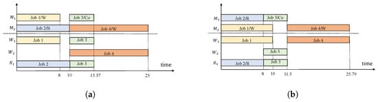
The actual processing time and worker fatigue are calculated according to the processing-time and fatigue-evolution models in Section 3.2 and Section 3.3. The parameters are set as ${\eta }_W=1$, ${\eta }_R=0.5$, ${\eta }_{\mathrm{Co}}=1.43$, ${\lambda }_f=0.03$, ${\mu }_f=0.02$, ${\beta }_f^W=0.2$, and ${\beta }_f^{\mathrm{Co}}=0.1$. Figure 3 presents the two schedules.

Figure 3. Two schedules for the illustrative example: (a) Schedule with better fatigue balance; (b) Schedule with shorter average flow time.

For the schedule in Figure 3a, the completion times of jobs $I_1$–$I_4$ are 8, 10, 13.57, and 25, respectively. The average flow time is calculated as follows:

$$f_1^a={\displaystyle \frac{(8-0)+(10-0)+(13.57-0)+(25-2)}{4}}=13.64.$$

(18)

The final fatigue levels of workers $W_1$ and $W_2$ are 0.3378 and 0.4500, respectively. Thus, the worker fatigue balance index is

$$f_2^a=\sqrt{{\displaystyle \frac{{(0.3378-0.3939)}^2+{(0.4500-0.3939)}^2}{2}}}=0.0561.$$

(19)

For the schedule in Figure 3b, jobs $I_2$ and $I_3$ are completed earlier, but jobs $I_1$ and $I_4$ are both assigned to worker $W_1$, leading to greater fatigue imbalance. The completion times of jobs $I_1$–$I_4$ are 10, 8, 11.5, and 25.79, respectively. The average flow time is

$$f_1^b={\displaystyle \frac{(10-0)+(8-0)+(11.5-0)+(25.79-2)}{4}}=13.32.$$

(20)

The final fatigue levels of workers $W_1$ and $W_2$ are 0.7736 and 0.1050, respectively. Accordingly, the worker fatigue balance index is

$$f_2^b=\sqrt{{\displaystyle \frac{{(0.7736-0.4393)}^2+{(0.1050-0.4393)}^2}{2}}}=0.3343.$$

(21)

To compare the two schedules under the composite objective, the representative intermediate weight $\omega =50$ is used in this example. According to $F=f_1+\omega f_2$, the objective values of the two schedules are 16.45 and 30.04, respectively.

Although the schedule in Figure 3b achieves a smaller average flow time, it concentrates more workload on worker $W_1$ and therefore yields a larger worker fatigue balance index. The reduction in average flow time is outweighed by the increase in fatigue imbalance, so the schedule in Figure 3a obtains a lower composite objective value. This comparison illustrates that scheduling decisions in the DPMS-HRC problem jointly affect production efficiency and fatigue management, and thus workstation assignment, processing-mode selection, and worker–robot resource allocation need to be coordinated.

4. AMPS-MAPPO Algorithm

4.1. AMPS-MAPPO Framework

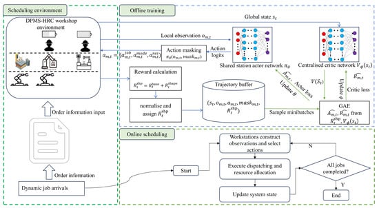
The overall AMPS-MAPPO framework for the DPMS-HRC problem is shown in Figure 4 and consists of the scheduling environment, offline training, and online scheduling. The environment maintains the current job, workstation, worker, robot, and worker-fatigue states and triggers scheduling decisions at job-arrival or job-completion events. Given the current environment state and scheduling actions, the next-state distribution is independent of earlier history, satisfying the Markov property. Since decisions are triggered by job-arrival and job-completion events and the elapsed time between consecutive decision epochs is variable, the scheduling process is formulated as an event-driven semi-Markov decision process (SMDP).

Figure 4. Framework of AMPS-MAPPO for the DPMS-HRC problem.

Each workstation is treated as an agent and makes a decision when it becomes idle with eligible jobs waiting. The shared actor selects a workstation-level scheduling action that jointly determines job selection, processing mode, and resource allocation. Detailed definitions of the local observation, global state, and action space are given in Section 4.2 and Section 4.3.

When multiple workstations become decision-ready at the same event time, their actions are generated through sequential micro-steps. Temporary reservations of selected jobs, workers, and robots are maintained within the decision epoch and update the feasible choices of subsequent workstation agents before the joint action set is committed. This mechanism coordinates workstation-level decisions under shared-resource constraints.

AMPS-MAPPO adopts centralised training and decentralised execution. All workstation agents share the actor network ${\pi }_{\theta }$ for action selection, while the centralised critic $V_{\varphi }$ evaluates the global state during training. After the selected assignments are executed, the environment advances to the next event and stores the resulting transitions for policy updates. During online scheduling, only the trained shared actor is retained for real-time decision-making.

The overall offline training procedure is summarised in Algorithm 1; the subsequent algorithms describe the micro-step decision, event-driven transition, reward assignment, and PPO update procedures.

4.2. Local Observation and Global State

For workstation m at decision time t, the local observation is denoted by $o_{m,t}=(o_1,o_2,\dots ,o_{17})$. It contains workstation status, candidate-job information, resource availability, fatigue-related information, system load, and time-related features, as shown in Table 4. The local observation is used by the shared station actor network for action selection.

Table 4. Local observation of each workstation agent.

Category	Symbol	Description
Workstation	$o_1$	1 if workstation m is idle, and 0 otherwise
	$o_2$	Remaining processing time of the current job on workstation m
Job	$o_3$	Minimum baseline processing time among candidate jobs
	$o_4$	Average baseline processing time among candidate jobs
Resource	$o_5$	Minimum fatigue level among available workers
	$o_6$	Average fatigue level of available workers
	$o_7$	Standard deviation of fatigue levels among all workers
	$o_8$	Range of fatigue levels among all workers
	$o_9$	Number of available workers
	$o_{10}$	Average remaining busy time of all workers
	$o_{11}$	Instantaneous busy ratio of all robots
	$o_{12}$	Average remaining busy time of all robots
	$o_{13}$	Number of available robots
Load	$o_{14}$	Number of global waiting jobs
	$o_{15}$	Number of candidate jobs for workstation m
Time	$o_{16}$	Current simulation time
	$o_{17}$	Time interval since the previous decision epoch

During centralised training, the critic uses an aggregated global-state representation obtained by concatenating the local observations of all workstations:

$$s_t={\left[o_{1,t}^{\top },o_{2,t}^{\top },\dots ,o_{\left|M\right|,t}^{\top }\right]}^{\top }.$$

The actor uses only the local observation $o_{m,t}$ for action selection, whereas the critic uses $s_t$ for state-value estimation during training. Since $s_t$ is obtained by concatenating the local observations of all workstations, its dimension is $17\left|M\right|$ for a system with $\left|M\right|$ workstations. Before being fed into the actor network, each local observation is standardised feature-wise using the running mean and variance estimated from training observations. The resulting values are clipped to $[-10,10]$ to limit extreme inputs. The running statistics are updated during training and kept fixed during evaluation and online scheduling.

Algorithm 1 Training procedure of AMPS-MAPPO

Input:  DPMS-HRC environment $\mathcal{E}$; shared station actor network ${\pi }_{\theta }$ with actor parameters $\theta$; centralised critic network $V_{\varphi }$ with critic parameters $\varphi$; maximum episodes $E_{\max }$; maximum decision steps per episode $T_{\max }$; PPO epochs $K_{\mathrm{PPO}}$; minibatch size $B_{\mathrm{mb}}$; discount factor ${\gamma }_{\mathrm{RL}}$; GAE parameter ${\lambda }_{\mathrm{GAE}}$; policy clip range ${ϵ}_{\mathrm{clip}}$; value loss coefficient $c_v$; entropy coefficient ${\alpha }_{\mathrm{ent}}$; actor learning rate ${\alpha }_{\theta }$; critic learning rate ${\alpha }_{\varphi }$; gradient clipping norm $g_{\max }$. Output:  Trained actor parameters $\theta$ and critic parameters $\varphi$.

1: Initialise ${\pi }_{\theta }$, $V_{\varphi }$, observation normaliser, and reward normaliser.   2: for  $e=1$  to  $E_{\max }$  do   3:     Reset $\mathcal{E}$, obtain the initial global state $s_0$, set $s_t\leftarrow s_0$, and set $done\leftarrow \mathrm{false}$.   4:     Initialise episode trajectory buffer ${\mathcal{D}}_e\leftarrow Ø$ and decision counter $n_{\mathrm{dec}}\leftarrow 0$.   5:     while not $done$ and $n_{\mathrm{dec}}<T_{\max }$ do   6:         Identify the current set of decision workstations $M_t^{\mathrm{dec}}$.   7:         if $M_t^{\mathrm{dec}}=Ø$ then   8:            Execute an empty action dictionary in $\mathcal{E}$ to advance the system and obtain $s_{t+\Delta t}$ and $done$.   9:            Set $s_t\leftarrow s_{t+\Delta t}$; no transition is stored because no workstation action is generated. 10:            continue 11:         end if 12:         Apply Algorithm 2 to obtain conflict-free action dictionary ${\mathcal{A}}_t$ and temporary transition set ${\mathcal{B}}_t$. 13:         Apply Algorithm 3 to commit ${\mathcal{A}}_t$ and obtain $s_{t+\Delta t}$, shaped reward $R_t^{\mathrm{shp}}$, and $done$. 14:         Apply Algorithm 4 to normalise $R_t^{\mathrm{shp}}$, assign it to ${\mathcal{B}}_t$ and update ${\mathcal{D}}_e$. 15:         $s_t\leftarrow s_{t+\Delta t}$ and set $n_{\mathrm{dec}}\leftarrow n_{\mathrm{dec}}+\left|{\mathcal{B}}_t\right|$. 16:     end while 17:     Apply Algorithm 5 to update $\theta$ and $\varphi$ using ${\mathcal{D}}_e$. 18: end for 19: return $\theta ,\varphi$.

4.3. Action Space

4.3.1. Rule-Combination Composite Action Space

After constructing the local observation, each decision workstation selects a scheduling action from a discrete rule-combination action space. The action of workstation m at time t is denoted by $a_{m,t}$. In this study, the production actions are constructed by combining a job selection rule, a processing mode, and a resource allocation rule:

$$a_{m,t}=(a_{m,t}^{\mathrm{job}},a_{m,t}^{\mathrm{mode}},a_{m,t}^{\mathrm{res}}).$$

(22)

In addition to these production actions, an independent IDLE action is included. Thus, the action space consists of $2\times 3\times 2+1=13$ discrete actions. The action components are shown in Table 5.

Table 5. Action space.

Action Component	Rule	Description
Job selection	SPT	Select the job with the shortest processing time
	FIFO	Select the job with the earliest arrival time
Processing mode	W	Worker mode
	R	Robot mode
	Co	human–robot collaborative mode
Resource allocation	ML	Select the lowest-fatigue worker or lowest-workload robot
	EA	Select the earliest available resource
Idle action	IDLE	Keep the workstation idle

4.3.2. Action Masking

In a dynamic scheduling environment, some rule combinations may be structurally infeasible at a given decision epoch. For example, a workstation cannot select a job outside its eligible set, and the collaborative mode cannot be selected when no robot is available. Therefore, an action masking mechanism is used to remove structurally infeasible actions before action sampling, while the IDLE action is retained only when no feasible production action is available.

For workstation m at time t, the environment generates a binary action mask ${mask}_{m,t}\in {\{0,1\}}^{13}$. If the qth action is structurally feasible, ${mask}_{m,t}^{\left(q\right)}=1$; otherwise, ${mask}_{m,t}^{\left(q\right)}=0$. The present study adopts a non-delay scheduling rule; therefore, if at least one structurally feasible production action exists, the IDLE action is masked. The shared station actor is a feed-forward neural network with three fully connected hidden layers, whose detailed configuration is reported in Section 5.1. Given the normalised local observation $o_{m,t}$, the actor outputs $z_{\theta }\left(o_{m,t}\right)\in {\mathbb{R}}^{13}$. Each component of $z_{\theta }\left(o_{m,t}\right)$ is an un-normalised preference score, or logit, associated with one of the 13 discrete actions. The action mask is applied to these logits before softmax normalisation. The masked policy is defined as

$${\pi }_{\theta }(a_{m,t}\mid o_{m,t},{mask}_{m,t})=\mathrm{Softmax}\left(z_{\theta }\left(o_{m,t}\right)+\log {mask}_{m,t}\right),$$

(23)

where $\log 0$ is treated as $-\infty$, so structurally infeasible actions receive zero probability after the softmax operation. When multiple workstations make decisions at the same event time, Algorithm 2 generates their actions sequentially and maintains temporary reservation sets for selected jobs, workers and robots. These reservations update the action masks of subsequent workstations within the same decision epoch, thereby avoiding resource conflicts before the action dictionary is committed.

4.3.3. Illustrative Example of Micro-Step Decision

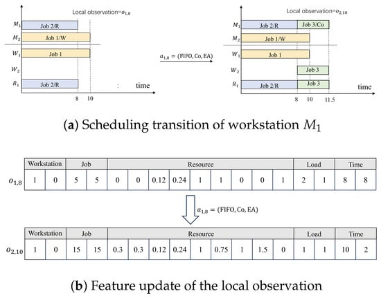
To illustrate the micro-step decision process, the small example in Table 3 is further used. The transition is explained based on Schedule b in Figure 3b. Figure 5 presents a representative decision of workstation $M_1$ and the corresponding update of the local observation.

Figure 5. Illustrative example of the micro-step decision process.

As shown in Figure 5a, when the system time reaches 8, workstation $M_1$ completes job $I_2$ and becomes available, thereby triggering a scheduling decision. Given the local observation $o_{1,8}$, the selected action is $a_{1,8}=(\mathrm{FIFO},\mathrm{Co},\mathrm{EA})$, which means that the next job is selected according to the FIFO rule, the collaborative mode is adopted, and the worker–robot pair is assigned according to the earliest-available rule. Accordingly, job $I_3$ is assigned to workstation $M_1$ and processed in Co mode by worker $W_2$ and robot $R_1$.

Algorithm 2 Micro-step decision with action masking

Input:  Global state $s_t$; current decision workstation set $M_t^{\mathrm{dec}}$; DPMS-HRC environment $\mathcal{E}$; shared station actor network ${\pi }_{\theta }$; centralised critic network $V_{\varphi }$; observation normaliser. Output:  Action dictionary ${\mathcal{A}}_t$; temporary transition set ${\mathcal{B}}_t$.

1: Initialise action dictionary ${\mathcal{A}}_t\leftarrow Ø$, temporary transition set ${\mathcal{B}}_t\leftarrow Ø$, and temporary reservation sets ${\mathcal{U}}_t^I,{\mathcal{U}}_t^W,{\mathcal{U}}_t^R\leftarrow Ø$.   2: Sort $M_t^{\mathrm{dec}}$ by ascending idle time, with ties broken by workstation index.   3: for each workstation $m\in M_t^{\mathrm{dec}}$ do   4:     Construct local observation $o_{m,t}$ for workstation m from $s_t$ and the current temporary reservations.   5:     Normalise $o_{m,t}$ using the observation normaliser.   6:     Generate action mask ${mask}_{m,t}$ by excluding infeasible actions under $s_t$ and the current temporary reservations.   7:     Estimate state value $v_t\leftarrow V_{\varphi }\left(s_t\right)$.   8:     Sample action $a_{m,t}$ from ${\pi }_{\theta }(·\mid o_{m,t},{mask}_{m,t})$ and record its log probability $\log p_{m,t}^{\mathrm{old}}$.   9:     Decode $a_{m,t}$ into a concrete assignment ${\xi }_{m,t}$ under the current temporary reservations. 10:     Add $(m,a_{m,t},{\xi }_{m,t})$ to ${\mathcal{A}}_t$. 11:     Update ${\mathcal{U}}_t^I,{\mathcal{U}}_t^W,{\mathcal{U}}_t^R$ according to ${\xi }_{m,t}$. 12:     Store $(o_{m,t},s_t,a_{m,t},{mask}_{m,t},\log p_{m,t}^{\mathrm{old}},v_t)$ in ${\mathcal{B}}_t$. 13: end for 14: return ${\mathcal{A}}_t,{\mathcal{B}}_t$.

After the selected assignment is committed to the environment, the system state is updated, and the event-driven environment advances to the next event time. In this example, the next event occurs at time 10, when workstation $M_2$ completes job $I_1$ and becomes available. Therefore, the next local observation considered by the actor changes from $o_{1,8}$ to $o_{2,10}$, as shown in Figure 5b. The updated observation reflects changes in workstation status, candidate-job information, resource availability, worker fatigue, system load, and time-related features.

This example illustrates how a local observation, a masked action, and the resulting worker–robot resource allocation are linked within one micro-step decision. It also shows how the event-driven mechanism updates the scheduling environment after the selected assignment is committed.

4.4. Reward Design

4.4.1. Base Reward

For an event-driven time interval $\Delta t$, the base reward considers the unfinished-job proportion $E\left(t\right)$, fatigue dispersion $B\left(t\right)$, fatigue range $G\left(t\right)$, high-fatigue risk $R^{\mathrm{risk}}\left(t\right)$, and delay term $D(t+\Delta t)$. Their detailed definitions are given in Table 6. The base reward is defined as follows:

$$\begin{array}{cc}\hfill R_t^{\mathrm{base}}=& -\left[{\rho }_{E}E\left(t\right)+{\rho }_B{\displaystyle \frac{B\left(t\right)}{F^{\max }}}+{\rho }_{G}G\left(t\right)+{\rho }_R{R}^{\mathrm{risk}}\left(t\right)\right]{\displaystyle \frac{\Delta t}{\tau }}-{\rho }_D\Delta tD(t+\Delta t).\hfill \end{array}$$

(24)

Table 6. Components of the base reward.

Component	Definition	Additional Notation
$E\left(t\right)$	${\displaystyle \frac{|I_t^{\mathrm{unf}}|}{\left|I\right|}}$	$I_t^{\mathrm{unf}}$: set of jobs that have arrived but have not been completed at time t.
$B\left(t\right)$	$\mathrm{Std}\{F_w\left(t\right):w\in W\}$	$F_w\left(t\right)$: fatigue level of worker w.
$G\left(t\right)$	${\displaystyle \frac{F_{\max }\left(t\right)-F_{\min }\left(t\right)}{F^{\max }}}$	$F_{\max }\left(t\right)$, $F_{\min }\left(t\right)$: maximum and minimum worker fatigue levels.
$R^{\mathrm{risk}}\left(t\right)$	${\displaystyle \frac{1}{\left|W\right|}}{\sum }_{w\in W}\mathrm{softplus}\left({\displaystyle \frac{F_w\left(t\right)-F^{\max }}{{\sigma }_{\mathrm{risk}}}}\right)$	${\sigma }_{\mathrm{risk}}$: risk sensitivity parameter.
$D(t+\Delta t)$	${\sum }_{i\in I^{\mathrm{late}}(t+\Delta t)}(t+\Delta t-d_i)$	$I^{\mathrm{late}}(t+\Delta t)$: late unfinished job set.

The base reward is designed to guide policy learning from intermediate scheduling states. Specifically, $E\left(t\right)$ measures the proportion of arrived but unfinished jobs, and its accumulation over event-driven intervals reflects the evolution of job flow time. The fatigue-related terms $B\left(t\right)$ and $G\left(t\right)$ describe the dispersion of worker fatigue during the scheduling process, thereby encouraging more balanced fatigue states. The risk penalty $R^{\mathrm{risk}}\left(t\right)$ penalises high-fatigue states relative to the operational threshold $F^{\max }$. The delay term $D(t+\Delta t)$ is used as an auxiliary signal to reduce excessive waiting and job starvation. These components provide process-level guidance for policy learning.

4.4.2. Time-Scaled Potential Shaping

To provide intermediate feedback for long-horizon scheduling, a potential function $\mathrm{\Phi }\left(s_t\right)$ is defined from the unfinished workload of arrived jobs. Let $p_i^{\min }={\min }_{m\in M_i}p{t}_{i,m}^{\mathrm{base}}$ denote the minimum base processing time of job $I_i$ among its eligible workstations:

$$\mathrm{\Phi }\left(s_t\right)=-{\eta }_p{\displaystyle \frac{{\sum }_{i\in I_t^{\mathrm{unf}}}{p}_i^{\min }}{{\sum }_{i\in I}{p}_i^{\min }}}.$$

(25)

To account for variable durations between event-driven decision epochs, the shaping reward uses the duration-dependent coefficient ${\mathrm{\Gamma }}_t={\gamma }_{\mathrm{RL}}^{\Delta t/\tau }$, where $\Delta t$ is the elapsed simulation time and $\tau$ is the time-scaling parameter:

$$R_t^{\mathrm{shape}}={\mathrm{\Gamma }}_t\mathrm{\Phi }\left(s_{t+\Delta t}\right)-\mathrm{\Phi }\left(s_t\right),{\mathrm{\Gamma }}_t={\gamma }_{\mathrm{RL}}^{\Delta t/\tau }.$$

(26)

This formulation retains the potential-difference structure of potential-based reward shaping, but ${\mathrm{\Gamma }}_t$ is used only in the shaping term, whereas PPO and GAE retain the fixed per-decision discount factor ${\gamma }_{\mathrm{RL}}$. The classical policy-invariance guarantee therefore does not directly apply to the present event-driven SMDP. The term is consequently treated as a time-scaled potential-shaping signal, whose effect is evaluated through the ablation experiments in Section 5.4.

The total shaped reward is

$$R_t^{\mathrm{shp}}=R_t^{\mathrm{base}}+R_t^{\mathrm{shape}}.$$

(27)

The reward parameters are set as ${\rho }_E=12.0$, ${\rho }_B=0.2$, ${\rho }_G=0.2$, ${\rho }_R=1.0$, ${\rho }_D=0.5$, ${\sigma }_{\mathrm{risk}}=0.2$, $\tau =10.0$, ${\eta }_p=0.2$, and ${\gamma }_{\mathrm{RL}}=0.99$, and are fixed across all experiments. Before trajectory storage, $R_t^{\mathrm{shp}}$ is normalised by the running standard deviation of the discounted return and clipped to $[-5,5]$. Algorithms 3 and 4 summarise the resulting reward calculation and assignment procedure.

Algorithm 3 Event-driven time advancement and reward calculation

Input:  DPMS-HRC environment $\mathcal{E}$ with simulation clock t and event queue $\mathcal{Q}$; action dictionary ${\mathcal{A}}_t$. Output:  Advanced global state $s_{t+\Delta t}$; shaped reward $R_t^{\mathrm{shp}}$; terminal flag $done$.

1: Commit the conflict-free assignments in ${\mathcal{A}}_t$ at the current decision time.   2: Lock the selected job, workstation, worker and robot resources in $\mathcal{E}$.   3: Compute the actual processing times and insert the corresponding completion events into $\mathcal{Q}$.   4: Record the potential value $\mathrm{\Phi }\left(s_t\right)$ before event-driven advancement.   5: Advance the simulation clock to the next job-arrival or job-completion event.   6: Process all concurrent events at the new event time and update job, workstation, worker and robot states.   7: Compute the base reward accumulated over the elapsed interval.   8: Obtain the advanced global state $s_{t+\Delta t}$ and compute $\mathrm{\Phi }\left(s_{t+\Delta t}\right)$.   9: Set the duration-dependent shaping coefficient ${\mathrm{\Gamma }}_t\leftarrow {\gamma }_{\mathrm{RL}}^{\Delta t/\tau }$. 10: Compute the shaped reward: $$R_t^{\mathrm{shp}}=R_t^{\mathrm{base}}+{\mathrm{\Gamma }}_t\mathrm{\Phi }\left(s_{t+\Delta t}\right)-\mathrm{\Phi }\left(s_t\right).$$ 11: Determine whether all jobs have been completed and update $done$. 12: return $s_{t+\Delta t},R_t^{\mathrm{shp}},done$.

Algorithm 4 Reward normalisation and trajectory storage

Input:  Temporary transition set ${\mathcal{B}}_t$; shaped reward $R_t^{\mathrm{shp}}$; terminal flag $done$; reward normaliser; episode trajectory buffer ${\mathcal{D}}_e$. Output:  Updated episode trajectory buffer ${\mathcal{D}}_e$.

1: if  ${\mathcal{B}}_t=Ø$  then   2:     return ${\mathcal{D}}_e$.   3: end if   4: Replace $R_t^{\mathrm{shp}}$ with its normalised value.   5: for each transition record $b\in {\mathcal{B}}_t$ do   6:     Retrieve $(o_{m,t},s_t,a_{m,t},{mask}_{m,t},\log p_{m,t}^{\mathrm{old}},v_t)$ from b.   7:     Assign the same normalised shaped reward $R_t^{\mathrm{shp}}$ to b.   8:     Append $(o_{m,t},s_t,a_{m,t},{mask}_{m,t},\log p_{m,t}^{\mathrm{old}},R_t^{\mathrm{shp}},done,v_t)$ to ${\mathcal{D}}_e$.   9: end for 10: return ${\mathcal{D}}_e$.

4.5. Actor and Critic Network Update

Each transition contains the local observation, global state, selected action, action mask, old log probability, normalised shaped reward, terminal flag, and critic value estimate. The advantage estimate ${\widehat{A}}_{m,t}$ and the target return ${\widehat{R}}_{m,t}$ are computed using GAE. The station actor network ${\pi }_{\theta }$ is updated using masked action probabilities, whereas the centralised critic network $V_{\varphi }$ is updated using global state values.

For a transition generated by workstation m at decision time t, the probability ratio is computed using the old log probability stored during trajectory collection:

$$r_{m,t}\left(\theta \right)=\exp \left[\log {\pi }_{\theta }(a_{m,t}\mid o_{m,t},{mask}_{m,t})-\log p_{m,t}^{\mathrm{old}}\right].$$

(28)

The clipped actor objective is defined as follows:

$$L^{\mathrm{clip}}\left(\theta \right)={\widehat{\mathbb{E}}}_{m,t}\left[\min \left(r_{m,t}\left(\theta \right){\widehat{A}}_{m,t},\mathrm{clip}\left(r_{m,t}\left(\theta \right),1-{ϵ}_{\mathrm{clip}},1+{ϵ}_{\mathrm{clip}}\right){\widehat{A}}_{m,t}\right)\right]+{\alpha }_{\mathrm{ent}}\mathcal{H}\left({\pi }_{\theta }\right).$$

(29)

For the centralised critic network, the value-function loss is defined as the mean-squared error between the predicted state value and the GAE target return:

$$L^{\mathrm{vf}}\left(\varphi \right)={\widehat{\mathbb{E}}}_{m,t}\left[{\left(V_{\varphi }\left(s_t\right)-{\widehat{R}}_{m,t}\right)}^2\right].$$

(30)

The GAE-based policy update procedure is summarised in Algorithm 5.

Algorithm 5 GAE-based PPO update

Input:  Episode trajectory buffer ${\mathcal{D}}_e$; shared station actor network ${\pi }_{\theta }$ with actor parameters $\theta$; centralised critic network $V_{\varphi }$ with critic parameters $\varphi$; PPO epochs $K_{\mathrm{PPO}}$; minibatch size $B_{\mathrm{mb}}$; discount factor ${\gamma }_{\mathrm{RL}}$; GAE parameter ${\lambda }_{\mathrm{GAE}}$; policy clip range ${ϵ}_{\mathrm{clip}}$; value loss coefficient $c_v$; entropy coefficient ${\alpha }_{\mathrm{ent}}$; actor learning rate ${\alpha }_{\theta }$; critic learning rate ${\alpha }_{\varphi }$; gradient clipping norm $g_{\max }$. Output:  Updated actor parameters $\theta$ and critic parameters $\varphi$.

1: Compute the advantage estimates and target returns, denoted by ${\widehat{A}}_{m,t}$ and ${\widehat{R}}_{m,t}$, for all transitions in ${\mathcal{D}}_e$ using GAE.   2: Normalise the advantage estimates.   3: for  $k=1$  to  $K_{\mathrm{PPO}}$  do   4:     Shuffle ${\mathcal{D}}_e$ and divide it into minibatches of size $B_{\mathrm{mb}}$.   5:     for each minibatch do   6:         Recompute masked log probabilities $\log {\pi }_{\theta }(a_{m,t}\mid o_{m,t},{mask}_{m,t})$.   7:         Compute the probability ratio: $$r_{m,t}\left(\theta \right)=\exp \left(\log {\pi }_{\theta }(a_{m,t}\mid o_{m,t},{mask}_{m,t})-\log p_{m,t}^{\mathrm{old}}\right).$$   8:         Compute the clipped actor objective using Equation (29).   9:         Compute the critic loss as $c_v{L}^{\mathrm{vf}}\left(\varphi \right)$ using Equation (30). 10:         Update actor parameters $\theta$ using learning rate ${\alpha }_{\theta }$ after gradient clipping by $g_{\max }$. 11:         Update critic parameters $\varphi$ using learning rate ${\alpha }_{\varphi }$ after gradient clipping by $g_{\max }$. 12:     end for 13: end for 14: return $\theta ,\varphi$.

5. Numerical Experiments and Results

All experiments were implemented in Python 3.12 on a Windows 11 computer with an Intel Core i5-12500H CPU at 2.50 GHz and 16 GB RAM. This section reports the convergence, arrival-rate sensitivity, comparative, statistical, and ablation results.

5.1. Experimental Settings and Parameter Configuration

Table 7, Table 8 and Table 9 report the training, environment, and scale settings. The learned policies are evaluated on separately generated test instances with seeds distinct from training; no test-set-specific hyperparameter tuning is performed, and the reported settings remain fixed across test configurations.

Table 7. Training hyperparameters of AMPS-MAPPO.

Parameter	Value	Parameter	Value
Actor hidden layers	256–256–256	Critic hidden layers	256–256–128
Max episodes	10,000	Max decision steps per episode	3000
Policy clip range	$0.2$	PPO epochs	4
Minibatch size	1024	Discount factor	$0.99$
GAE parameter	$0.95$	Value loss coefficient	$0.5$
Entropy coefficient	$0.01$	Gradient clip norm	$0.5$
Actor learning rate	$3\times {10}^{-4}$	Critic learning rate	$5\times {10}^{-4}$
Reward clip range	$5.0$

Table 8. Environment parameters.

Parameter	Value
Base processing time	Discrete uniform $U[10,30]$
Eligible workstations	Discrete uniform $U\left[\max \right(2,\lfloor \left|M\right|/3\rfloor ),|M\left|\right]$
Mode efficiency factor	${\eta }_W=1$, ${\eta }_R=0.5$, ${\eta }_{\mathrm{Co}}=1.43$
Fatigue-risk threshold	0.8
Fatigue accumulation rate	0.03
Fatigue recovery rate	0.02
Fatigue impact factor	${\beta }_f^W=0.2$, ${\beta }_f^{\mathrm{Co}}=0.1$

Table 9. Scale  settings.

Scale	Workstations M	Workers W	Robots R	Initial jobs ${\mathit{J}}_0$	Dynamic jobs ${\mathit{J}}_{\mathit{d}}$
Small	5	4	2	5	25
Medium	10	8	4	10	50
Large	30	24	10	10	100

The fatigue-related parameters in Table 8 are used as fixed simulation settings across all experiments rather than as empirically calibrated physiological coefficients.

5.2. Convergence and Arrival-Rate Sensitivity Analysis

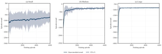
To assess training variability, AMPS-MAPPO was independently trained with seeds 42, 1042, and 2042 at $\lambda =0.067$ for each problem scale. Episode rewards were smoothed using a 100-episode moving average, and Figure 6 reports the across-seed mean and 95% Student’s t confidence interval.

Figure 6. Multi-seed training curves of AMPS-MAPPO for three problem scales.

Figure 6 shows rapid early improvement followed by stable rewards at all three scales. The medium- and large-scale settings have narrower confidence intervals, while the small-scale setting shows greater between-seed variability.

Arrival-rate sensitivity is evaluated at $\lambda =0.05$, $0.067$, and $0.10$ for all three problem scales using 20 independently generated test instances per setting and common test seeds across arrival rates. Table 10 reports $f_1$ and $f_2$.

Table 10. Effect of job arrival rate on AMPS-MAPPO performance.

Scale	$\mathit{\lambda }$	${\mathit{f}}_1$	${\mathit{f}}_2$
Small	0.050	22.48	0.4096
Small	0.067	26.30	0.4047
Small	0.100	41.05	0.3921
Medium	0.050	16.03	0.4428
Medium	0.067	16.65	0.4643
Medium	0.100	18.19	0.4915
Large	0.050	13.94	0.3854
Large	0.067	14.26	0.3669
Large	0.100	20.66	0.5098

Table 10 shows that $f_1$ increases with the arrival rate at all three scales, whereas $f_2$ varies non-monotonically: it decreases in the small-scale setting, increases in the medium-scale setting, and first decreases and then increases in the large-scale setting. This difference arises because $f_2$ measures end-of-horizon fatigue dispersion rather than workload intensity.

5.3. Comparative Experiments

Each configuration is evaluated on 20 independently generated test instances matched across methods by test seed. Comparisons report $f_1$ and $f_2$ separately, while the composite objective is used only where a common reference weight is required.

5.3.1. Comparison with Gurobi Under Small-Scale Settings

AMPS-MAPPO is compared with Gurobi at the reference weight $\omega =50$. The fixed AMPS-MAPPO policy is scored ex post, while Gurobi uses a 300 s time limit, a relative MIP gap of 0.10, and NonConvex = 2. Table 11 reports objective values and computational times. Gurobi reports the best incumbent within the time limit, so optimality is not guaranteed; AMPS-MAPPO time refers only to online inference.

Table 11. Comparison with Gurobi.

$(\mathit{M},{\mathit{J}}_0,\mathit{\lambda },\mathit{R},\mathit{W})$	${\mathit{J}}_{\mathit{d}}$	Algorithm	Objective Value at $\mathit{\omega }=50$	Computational Time
(5, 5, 0.05, 1, 1)	10	AMPS-MAPPO	116.01	0.213 ms
		Gurobi	94.20	300.12 s
	15	AMPS-MAPPO	132.44	0.277 ms
		Gurobi	106.03	300.16 s
	20	AMPS-MAPPO	148.44	0.430 ms
		Gurobi	118.87	300.16 s
(5, 5, 0.05, 1, 2)	10	AMPS-MAPPO	77.84	0.253 ms
		Gurobi	77.16	300.14 s
	15	AMPS-MAPPO	80.19	0.261 ms
		Gurobi	85.80	303.65 s
	20	AMPS-MAPPO	90.03	0.343 ms
		Gurobi	112.88	301.37 s
(5, 5, 0.05, 1, 3)	10	AMPS-MAPPO	60.46	0.130 ms
		Gurobi	65.26	315.47 s
	15	AMPS-MAPPO	63.13	0.180 ms
		Gurobi	74.33	307.54 s
	20	AMPS-MAPPO	65.58	0.244 ms
		Gurobi	80.11	300.20 s

At $\omega =50$, Gurobi obtains lower objective values in all three one-worker settings, whereas AMPS-MAPPO obtains lower values in five of the six settings with two or three workers. Gurobi generally approaches the 300 s time limit, while AMPS-MAPPO retains millisecond-level online inference.

5.3.2. Comparison with Rule-Based Dispatching Methods

AMPS-MAPPO is compared with 12 rule-based dispatching methods over 24 medium- and large-scale configurations. Table 12 reports $f_1$ and $f_2$.

Table 12. Comparison with rule-based dispatching methods.

$(\mathit{M},{\mathit{J}}_0,\mathit{\lambda },\mathit{R},\mathit{W})$	${\mathit{J}}_{\mathit{d}}$	Metric	AMPS-MAPPO	SPT-Based Rules						FIFO-Based Rules
				W–ML	W–EA	R–ML	R–EA	Co–ML	Co–EA	W–ML	W–EA	R–ML	R–EA	Co–ML	Co–EA
(10, 10, 0.10, 3, 3)	30	$f_1$	50.99	411.47	411.26	110.55	110.55	266.45	265.77	493.90	494.00	160.29	160.29	337.67	338.62
		$f_2$	0.3715	0.7426	0.7435	–	–	0.5111	0.5054	0.6646	0.6642	–	–	0.4547	0.4774
	40	$f_1$	51.92	511.57	511.36	119.11	119.11	332.68	332.54	617.20	617.68	178.34	178.34	417.41	417.40
		$f_2$	0.3469	0.7011	0.7013	–	–	0.4981	0.4933	0.6946	0.6911	–	–	0.4715	0.4733
	50	$f_1$	51.68	614.17	612.78	127.66	127.66	398.61	399.50	741.59	742.11	195.88	195.88	500.23	500.22
		$f_2$	0.4012	0.7257	0.7142	–	–	0.4723	0.4803	0.5626	0.5582	–	–	0.3898	0.3913
(10, 10, 0.10, 2, 4)	30	$f_1$	63.04	257.11	256.98	226.19	226.19	173.96	175.06	329.53	329.61	293.74	293.74	221.82	220.88
		$f_2$	0.3924	0.6529	0.6671	–	–	0.4349	0.4525	0.7014	0.6999	–	–	0.4266	0.4242
	40	$f_1$	67.41	321.38	321.65	260.99	260.99	212.67	213.73	408.71	408.77	345.00	345.00	272.00	271.27
		$f_2$	0.4340	0.6874	0.7007	–	–	0.4752	0.4777	0.6786	0.6415	–	–	0.4515	0.4272
	50	$f_1$	70.64	383.57	384.40	296.60	296.60	252.54	253.39	487.25	486.96	396.08	396.08	323.58	323.17
		$f_2$	0.4465	0.6779	0.6707	–	–	0.4750	0.4748	0.6053	0.5982	–	–	0.4059	0.4105
(10, 10, 0.10, 2, 6)	30	$f_1$	32.05	257.11	256.98	65.61	65.61	150.12	150.13	329.53	329.61	98.57	98.57	210.67	210.57
		$f_2$	0.3274	0.6529	0.6671	–	–	0.4418	0.4417	0.7014	0.6999	–	–	0.4628	0.4559
	40	$f_1$	32.34	321.38	321.65	65.84	65.84	186.25	186.27	408.71	408.77	101.63	101.63	258.70	258.49
		$f_2$	0.3050	0.6874	0.7007	–	–	0.4936	0.4797	0.6786	0.6415	–	–	0.4472	0.4479
	50	$f_1$	32.18	383.57	384.40	65.35	65.35	219.90	221.32	487.25	486.96	103.98	103.98	309.06	309.18
		$f_2$	0.3286	0.6779	0.6707	–	–	0.4420	0.4596	0.6053	0.5982	–	–	0.4594	0.4326
(10, 10, 0.10, 2, 6)	30	$f_1$	33.87	109.14	108.88	226.19	226.19	78.37	78.21	163.50	163.67	293.74	293.74	102.23	101.53
		$f_2$	0.4443	0.7302	0.7404	–	–	0.4663	0.4831	0.6956	0.6948	–	–	0.4572	0.4661
	40	$f_1$	35.33	133.41	133.11	260.99	260.99	91.42	90.59	199.60	200.04	345.00	345.00	118.48	118.82
		$f_2$	0.4895	0.7298	0.6840	–	–	0.4856	0.4826	0.6716	0.7005	–	–	0.4338	0.4922
	50	$f_1$	35.88	157.26	156.23	296.60	296.60	104.28	103.23	236.81	237.54	396.08	396.08	135.08	135.71
		$f_2$	0.4598	0.7092	0.7538	–	–	0.4893	0.4755	0.6730	0.6574	–	–	0.4629	0.4511
(20, 20, 0.07, 6, 6)	80	$f_1$	23.60	181.59	180.25	47.04	47.04	61.05	60.20	310.52	311.82	58.70	58.70	122.50	124.10
		$f_2$	0.4087	0.7439	0.7625	–	–	0.4738	0.4526	0.7098	0.7237	–	–	0.4611	0.4450
	100	$f_1$	22.66	191.90	190.31	46.18	46.18	57.22	56.38	335.58	337.25	55.90	55.90	115.73	117.02
		$f_2$	0.4149	0.7934	0.7564	–	–	0.4631	0.4467	0.7233	0.6972	–	–	0.4950	0.4789
	120	$f_1$	22.09	200.61	199.86	45.43	45.43	54.89	54.02	360.63	363.21	53.78	53.78	111.33	112.63
		$f_2$	0.4183	0.7524	0.7524	–	–	0.4830	0.5125	0.7281	0.7148	–	–	0.4644	0.4688
(20, 20, 0.07, 4, 8)	80	$f_1$	22.53	55.23	55.49	66.74	66.74	28.74	28.78	108.33	109.66	95.23	95.23	44.13	44.27
		$f_2$	0.4199	0.6678	0.6604	–	–	0.4277	0.4333	0.6798	0.6852	–	–	0.4226	0.4341
	100	$f_1$	21.32	51.89	52.47	63.09	63.09	26.55	26.58	101.60	103.19	87.35	87.35	39.45	39.56
		$f_2$	0.4425	0.7380	0.7339	–	–	0.4668	0.4781	0.7102	0.7365	–	–	0.4645	0.4705
	120	$f_1$	20.49	49.44	50.50	60.58	60.58	24.98	25.14	96.95	98.55	81.86	81.86	36.06	36.30
		$f_2$	0.4365	0.6578	0.6609	–	–	0.4384	0.4422	0.6551	0.6342	–	–	0.4387	0.4450
(20, 20, 0.07, 8, 8)	80	$f_1$	18.48	55.23	55.49	42.75	42.75	22.36	22.26	108.33	109.66	49.42	49.42	39.27	38.89
		$f_2$	0.4157	0.6678	0.6604	–	–	0.4286	0.4357	0.6798	0.6852	–	–	0.4344	0.4347
	100	$f_1$	17.94	51.89	52.47	42.51	42.51	21.22	21.11	101.60	103.19	48.07	48.07	35.45	35.04
		$f_2$	0.4435	0.7380	0.7339	–	–	0.4657	0.4787	0.7102	0.7365	–	–	0.4643	0.4686
	120	$f_1$	17.58	49.44	50.50	42.23	42.23	20.41	20.43	96.95	98.55	46.99	46.99	32.64	32.41
		$f_2$	0.4252	0.6578	0.6609	–	–	0.4353	0.4369	0.6551	0.6342	–	–	0.4356	0.4310
(20, 20, 0.07, 4, 12)	80	$f_1$	17.77	22.72	22.74	66.74	66.74	18.97	18.98	32.26	32.28	95.23	95.23	23.71	23.68
		$f_2$	0.3922	0.5815	0.5868	–	–	0.3933	0.3964	0.5906	0.5940	–	–	0.3940	0.3969
	100	$f_1$	17.21	22.50	22.52	63.09	63.09	18.21	18.22	30.46	30.48	87.35	87.35	22.16	22.14
		$f_2$	0.4362	0.6480	0.6488	–	–	0.4324	0.4385	0.6485	0.6485	–	–	0.4324	0.4385
	120	$f_1$	16.83	22.23	22.25	60.58	60.58	17.68	17.69	29.05	29.06	81.86	81.86	21.07	21.05
		$f_2$	0.4046	0.5661	0.5728	–	–	0.3976	0.4040	0.5661	0.5728	–	–	0.3976	0.4040

Note: f₂ is not applicable to pure robot rules because no worker is assigned.

AMPS-MAPPO achieves the lowest $f_1$ in all 24 configurations, with an overall mean of 33.16. Some collaborative-mode rules obtain comparable or lower $f_2$ values in individual configurations, but generally with longer flow times. The results therefore show a clear scheduling-efficiency advantage for AMPS-MAPPO while retaining competitive fatigue-balance performance.

5.3.3. Comparison with Baseline Reinforcement Learning Algorithms

DQN, PPO, SAC, and D3QN are used as reinforcement-learning baselines. All methods use the same DPMS-HRC environment, 17-dimensional local observation, 13-action definition, reward specification, 10,000-episode training horizon, and matched test instances. The baselines are trained with seed 42 and evaluated on the same 20 test-instance seeds per configuration, distinct from training, without test-set-specific hyperparameter tuning. All use a learning rate of $3\times {10}^{-4}$. PPO and D3QN incorporate feasibility during action selection. DQN and SAC do not mask infeasible actions during training; the environment handles them without resampling or an additional penalty. During evaluation, an infeasible DQN or SAC action is replaced by IDLE when feasible, or otherwise by the first feasible action. SAC uses a one-dimensional Gaussian policy over $[0,12]$, whose output is rounded and clipped to the 13 discrete actions. DQN uses a $2\times 256$ ReLU Q-network, batch size 256, replay buffer $3\times {10}^5$, one update per step, and target updates every 500 steps. PPO uses $2\times 256$ Tanh policy and value networks, rollout and minibatch size 2048, and four update epochs. SAC uses a $2\times 256$ ReLU Gaussian actor and twin Q-networks, batch size 1024, replay buffer $3\times {10}^5$, four updates every four steps, $\tau =0.005$, and automatic entropy tuning. D3QN uses a $2\times 256$ ReLU feature network with duelling heads, batch size 256, replay buffer $1.2\times {10}^5$, one update per step, and target updates every 500 steps.

AMPS-MAPPO obtains the lowest $f_1$ in 18 of 24 configurations and the lowest overall mean of 31.78, corresponding to mean reductions of 20.92%, 12.06%, 8.17%, and 13.59% relative to DQN, PPO, SAC, and D3QN. For $f_2$, it also achieves the lowest overall mean (0.4365), although AMPS-MAPPO and D3QN each obtain the lowest value in 10 configurations. Thus, the flow-time advantage is more consistent than the fatigue-balance advantage.

5.3.4. Process-Level Fatigue Analysis

Four process-level indicators supplement $f_2$: maximum fatigue, time-above-threshold ratio, cumulative fatigue exposure, and temporal workload dispersion. The latter is the mean cross-worker standard deviation of utilisation over ten equal intervals of the scheduling horizon. Results are summarised over the same 24 medium- and large-scale configurations used in Table 12 and Table 13.

Table 13. Comparison with baseline reinforcement learning algorithms.

$(\mathit{M},{\mathit{J}}_0,\mathit{\lambda },\mathit{R},\mathit{W})$	${\mathit{J}}_{\mathit{d}}$	Metric	AMPS-MAPPO	DQN	PPO	SAC	D3QN
(10, 10, 0.10, 3, 3)	30	$f_1$	49.62	59.59	53.93	49.92	47.95
		$f_2$	0.4082	0.3595	0.4255	0.3458	0.4666
	40	$f_1$	49.19	59.42	52.91	49.88	48.22
		$f_2$	0.4520	0.4138	0.4931	0.4843	0.4081
	50	$f_1$	49.30	59.33	52.89	50.02	48.33
		$f_2$	0.2343	0.3792	0.3672	0.4829	0.5129
(10, 10, 0.10, 2, 4)	30	$f_1$	61.31	73.62	63.96	57.65	56.63
		$f_2$	0.4978	0.5086	0.5239	0.5073	0.5708
	40	$f_1$	63.30	75.10	65.73	59.31	58.16
		$f_2$	0.5199	0.3812	0.4684	0.5413	0.5391
	50	$f_1$	65.20	77.05	67.42	61.10	59.91
		$f_2$	0.5028	0.4541	0.4972	0.5857	0.6040
(10, 10, 0.10, 4, 4)	30	$f_1$	32.21	39.40	36.73	34.94	33.34
		$f_2$	0.3418	0.2919	0.5599	0.4794	0.5540
	40	$f_1$	31.90	39.08	37.13	35.18	33.73
		$f_2$	0.3102	0.5114	0.4548	0.4781	0.5276
	50	$f_1$	31.67	38.74	37.16	35.49	34.01
		$f_2$	0.4030	0.4925	0.4596	0.4069	0.6392
(10, 10, 0.10, 2, 6)	30	$f_1$	33.82	43.15	36.31	35.50	34.68
		$f_2$	0.4780	0.5394	0.6044	0.5610	0.5696
	40	$f_1$	33.85	42.84	36.98	36.40	35.27
		$f_2$	0.4881	0.5524	0.5523	0.5700	0.5470
	50	$f_1$	34.62	42.84	38.00	36.48	35.83
		$f_2$	0.4745	0.5104	0.5158	0.5929	0.5896
(20, 20, 0.07, 6, 6)	80	$f_1$	22.34	30.10	27.31	27.31	32.73
		$f_2$	0.4632	0.5913	0.6427	0.6430	0.3866
	100	$f_1$	21.55	29.55	27.21	27.20	32.69
		$f_2$	0.4658	0.6136	0.6099	0.6106	0.3631
	120	$f_1$	21.11	29.25	27.17	27.16	32.63
		$f_2$	0.4222	0.6178	0.5975	0.5975	0.3213
(20, 20, 0.07, 4, 8)	80	$f_1$	20.99	28.21	24.78	24.83	30.04
		$f_2$	0.4566	0.6446	0.6235	0.6238	0.4043
	100	$f_1$	19.93	27.43	24.51	24.55	30.05
		$f_2$	0.4775	0.6326	0.6430	0.6430	0.4352
	120	$f_1$	19.30	27.03	24.37	24.41	30.14
		$f_2$	0.4642	0.5913	0.5971	0.5979	0.3927
(20, 20, 0.07, 8, 8)	80	$f_1$	17.66	25.25	23.48	23.43	30.05
		$f_2$	0.4596	0.6376	0.6234	0.6219	0.3418
	100	$f_1$	17.14	24.98	23.42	23.39	30.42
		$f_2$	0.4632	0.6202	0.6430	0.6361	0.3519
	120	$f_1$	16.89	24.91	23.46	23.43	30.60
		$f_2$	0.4557	0.6061	0.5947	0.5810	0.3155
(20, 20, 0.07, 4, 12)	80	$f_1$	16.99	22.62	20.80	21.02	25.30
		$f_2$	0.4074	0.5532	0.5987	0.5982	0.4548
	100	$f_1$	16.51	22.41	20.76	20.95	25.84
		$f_2$	0.4225	0.5391	0.6098	0.6094	0.4291
	120	$f_1$	16.20	22.53	20.81	20.97	26.04
		$f_2$	0.4088	0.5169	0.5712	0.5708	0.4457

Table 14 shows that AMPS-MAPPO has the lowest time-above-threshold ratio in both groups and the lowest cumulative fatigue exposure in the large group. Collaborative-mode rules perform better on some other fatigue indicators, particularly maximum fatigue and temporal workload dispersion.

Table 14. Process-level fatigue indicators for AMPS-MAPPO and rule-based methods.

Configuration Group	Method	Maximum Fatigue	Time-Above-Threshold Ratio	Cumulative Fatigue Exposure	Temporal Workload Dispersion
Medium $(M,J_0,\lambda )=(10,10,0.10)$	AMPS-MAPPO	2.907	0.853	1.276	0.131
	SPT-W-ML	3.000	0.914	1.442	0.064
	SPT-W-EA	3.000	0.914	1.442	0.065
	SPT-Co-ML	2.535	0.878	1.226	0.059
	SPT-Co-EA	2.535	0.879	1.228	0.059
	FIFO-W-ML	3.000	0.914	1.470	0.064
	FIFO-W-EA	3.000	0.913	1.470	0.065
	FIFO-Co-ML	2.532	0.881	1.239	0.057
	FIFO-Co-EA	2.537	0.881	1.239	0.057
Large $(M,J_0,\lambda )=(20,20,0.07)$	AMPS-MAPPO	2.801	0.415	0.764	0.040
	SPT-W-ML	3.000	0.705	1.172	0.049
	SPT-W-EA	3.000	0.705	1.171	0.049
	SPT-Co-ML	2.476	0.485	0.823	0.038
	SPT-Co-EA	2.484	0.487	0.823	0.039
	FIFO-W-ML	3.000	0.753	1.262	0.049
	FIFO-W-EA	3.000	0.750	1.259	0.050
	FIFO-Co-ML	2.511	0.536	0.882	0.038
	FIFO-Co-EA	2.524	0.537	0.882	0.039

Table 15 shows that AMPS-MAPPO achieves the lowest maximum fatigue and temporal workload dispersion in both groups. PPO gives the lowest time-above-threshold ratio and cumulative exposure in the medium group, whereas D3QN gives the lowest values for these two indicators in the large group.

Table 15. Process-level fatigue indicators for AMPS-MAPPO and reinforcement-learning baselines.

Configuration Group	Method	Maximum Fatigue	Time-Above-Threshold Ratio	Cumulative Fatigue Exposure	Temporal Workload Dispersion
Medium $(M,J_0,\lambda )=(10,10,0.10)$	AMPS-MAPPO	2.901	0.853	1.284	0.132
	DQN	2.985	0.818	1.308	0.136
	PPO	2.975	0.773	1.252	0.142
	SAC	2.982	0.850	1.348	0.150
	D3QN	2.996	0.826	1.348	0.153
Large $(M,J_0,\lambda )=(20,20,0.07)$	AMPS-MAPPO	2.855	0.415	0.765	0.042
	DQN	2.994	0.552	0.996	0.055
	PPO	2.996	0.581	1.041	0.054
	SAC	2.994	0.577	1.033	0.054
	D3QN	2.929	0.257	0.546	0.059

5.3.5. Weight Sensitivity and Instance-Level Statistical Analysis

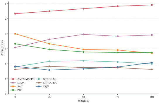
Weight sensitivity is examined by recalculating $F=f_1+\omega f_2$ from unchanged scheduling outcomes; $\omega$ therefore affects only the ex-post evaluation, not the trained policy.

Figure 7 shows that AMPS-MAPPO maintains the lowest average ranking among the compared learning and rule-based methods over the examined weight range. As the midpoint of the examined weight range, $\omega =50$ is used as a representative reference setting for the composite-objective comparisons rather than as an optimal weight.

Figure 7. Average rankings under different weight settings.

Paired statistical comparisons are conducted separately within each of the 24 configurations using 20 independently generated test instances matched across methods by test seed. For each objective and baseline, a two-sided Wilcoxon signed-rank test with Holm correction is applied within the corresponding method family; 95% Student’s t confidence intervals for paired mean differences and matched-pairs rank-biserial correlations are also reported.

For $f_1$, AMPS-MAPPO is significantly better than both representative rules and DQN in all 24 configurations, PPO in 21, SAC in 16, and D3QN in 15, with median rank-biserial correlations of 0.895–1.000. For $f_2$, significant advantages occur against DQN, PPO, and SAC in 13, 14, and 14 configurations, while the D3QN comparison is more balanced. Thus, the flow-time advantage is stronger and more consistent than the fatigue-balance advantage.

Table 16 summarises the configuration-level paired statistical comparisons.

Table 16. Configuration-level paired statistical comparisons with AMPS-MAPPO.

Family	Baseline	Objective	Better	Worse	Median Effect Size
Rules	SPT-Co-ML	$f_1$	24	0	1.000
		$f_2$	6	0	0.386
	SPT-Co-EA	$f_1$	24	0	1.000
		$f_2$	6	0	0.405
RL	DQN	$f_1$	24	0	1.000
		$f_2$	13	0	0.671
	PPO	$f_1$	21	0	1.000
		$f_2$	14	0	0.738
	SAC	$f_1$	16	2	0.981
		$f_2$	14	0	0.748
	D3QN	$f_1$	15	3	0.895
		$f_2$	3	3	0.114

Note: “Better” and “Worse” indicate significantly lower and higher AMPS-MAPPO objective values, respectively, after Holm correction ($p<0.05$); positive effect sizes favour AMPS-MAPPO.

5.4. Ablation Experiments

AMPS-MAPPO is compared with variants without action masking, without reward shaping, and without both mechanisms, while retaining the same shared-actor and centralised-critic architecture. In the no-mask variant, all 13 actions remain selectable; infeasible production actions are neither resampled nor separately penalised and result in no assignment in the current micro-step.

Table 17 reports the ablation results.

Table 17. Ablation experiment results.

$(\mathit{M},{\mathit{J}}_0,\mathit{\lambda },\mathit{R},\mathit{W})$	${\mathit{J}}_{\mathit{d}}$	Metric	AMPS-MAPPO	Without Action Masking	Without Reward Shaping	Without Both
(5, 5, 0.05, 1, 2)	10	$f_1$	64.34	110.09	69.76	127.39
		$f_2$	0.3455	0.3347	0.2961	0.0126
	15	$f_1$	69.33	142.25	75.69	150.10
		$f_2$	0.4545	0.2883	0.2520	0.0018
	20	$f_1$	75.03	174.23	80.34	167.63
		$f_2$	0.4027	0.2366	0.3726	0.0011
(5, 5, 0.05, 1, 3)	10	$f_1$	38.11	56.97	43.27	114.08
		$f_2$	0.4180	0.4503	0.2490	0.0223
	15	$f_1$	40.58	64.87	45.21	136.76
		$f_2$	0.5318	0.4025	0.4843	0.0028
	20	$f_1$	42.38	73.02	45.60	155.96
		$f_2$	0.4957	0.4010	0.4464	0.0072
(10, 10, 0.10, 2, 4)	30	$f_1$	63.04	206.12	80.49	85.63
		$f_2$	0.3924	0.5711	0.4308	0.4712
	40	$f_1$	67.41	261.83	85.45	93.19
		$f_2$	0.4340	0.6530	0.4990	0.4107
	50	$f_1$	70.64	315.90	88.90	97.46
		$f_2$	0.4465	0.6494	0.4304	0.4809
(10, 10, 0.10, 2, 6)	30	$f_1$	33.87	73.99	46.42	47.77
		$f_2$	0.4443	0.5421	0.5041	0.4911
	40	$f_1$	35.33	86.41	46.54	49.09
		$f_2$	0.4895	0.6425	0.4856	0.4850
	50	$f_1$	35.88	98.91	46.13	49.94
		$f_2$	0.4598	0.5926	0.5410	0.4573
(20, 20, 0.067, 4, 8)	80	$f_1$	21.54	40.06	39.97	27.48
		$f_2$	0.4153	0.4333	0.2477	0.4627
	100	$f_1$	20.49	25.27	39.55	26.72
		$f_2$	0.4427	0.4563	0.2857	0.5278
	120	$f_1$	19.77	23.10	39.18	26.28
		$f_2$	0.4406	0.4382	0.2056	0.5054
(20, 20, 0.067, 4, 12)	80	$f_1$	16.35	40.45	36.35	25.08
		$f_2$	0.4062	0.2594	0.2449	0.5145
	100	$f_1$	16.10	38.76	36.54	24.82
		$f_2$	0.4417	0.2771	0.2689	0.5399
	120	$f_1$	15.89	37.60	36.61	24.43
		$f_2$	0.4031	0.2927	0.2819	0.5020
Mean	–	$f_1$	41.45	103.88	54.56	79.43
		$f_2$	0.4369	0.4401	0.3626	0.3276

AMPS-MAPPO achieves the lowest $f_1$ in all 18 settings, with a mean of 41.45 versus 103.88, 54.56, and 79.43 without action masking, reward shaping, and both mechanisms, respectively. The corresponding mean $f_2$ values are 0.4369, 0.4401, 0.3626, and 0.3276, confirming that fatigue balance varies non-monotonically across the ablations.

6. Discussion

6.1. Main Findings and Relation to Previous Studies

The numerical results show that AMPS-MAPPO has its most consistent advantage in average flow time, achieving the lowest $f_1$ in all rule-based comparisons and in most reinforcement-learning comparisons. In contrast, fatigue-related performance is more configuration-dependent. AMPS-MAPPO obtains favourable overall results for $f_2$, maximum fatigue, and temporal workload dispersion, but other methods achieve better values for some fatigue indicators in individual configurations. These results show that scheduling efficiency and fatigue-related performance do not necessarily improve in the same manner and should therefore be considered jointly.

Compared with previous HRC scheduling studies that mainly address task and resource coordination, and fatigue-aware scheduling studies that focus on worker fatigue or ergonomic factors, the present problem combines dynamic job arrivals, fatigue-dependent processing times, alternative human–robot processing modes, and shared resources in a parallel-workstation environment [12,20,30]. The event-driven multi-agent framework represents these coupled decisions at the workstation level, while sequential micro-steps coordinate competition for shared workers and robots at the same decision epoch.

The sensitivity and ablation results further clarify the behaviour of the proposed framework. Increasing the job-arrival rate consistently increases average flow time, whereas the fatigue balance index varies with problem scale. In the ablation experiments, the complete AMPS-MAPPO framework achieves the lowest $f_1$ in all examined settings, while $f_2$ changes non-monotonically when action masking or reward shaping is removed. This again indicates that improvements in flow-time performance do not necessarily correspond to improvements in fatigue balance.

6.2. Managerial Implications

The results suggest that human–robot resource planning should consider resource composition as well as production scale. Across the examined configurations, similar total resource levels can produce different flow-time performance under different worker–robot combinations. Therefore, resource planning should consider how workers and robots jointly support the available processing modes under the expected workload, rather than relying only on the total number of resources.

The results also indicate that scheduling efficiency and fatigue-related performance should be evaluated together. Methods that perform well in average flow time do not always achieve the best final fatigue balance or process-level fatigue indicators, and their relative performance varies across fatigue measures and configurations. The weight $\omega$ therefore represents an ex-post evaluation preference for this trade-off rather than a universally optimal setting. Since the present results are based on simulated scenarios and a scheduling-level fatigue model, application to a specific shop floor would require calibration using plant-specific processing and worker data.

6.3. Limitations and Future Research

Several limitations define the scope of the present results. Workers and robots are assumed to be homogeneous within their respective resource pools, inter-workstation transfer times are neglected, and dynamic job arrivals follow a Poisson process. Worker fatigue is represented by a scheduling-level accumulation and recovery model rather than by direct physiological measurements, and the current experiments do not consider machine failures, material shortages, or stochastic processing-time disturbances. Future research could therefore examine heterogeneous worker and robot capabilities, explicit transfer processes, more general arrival distributions, task-dependent worker states, additional production disturbances, and richer fatigue information obtained from shop-floor observations or sensors. Recent studies also illustrate possible sensing and recognition pathways for measured human-state information. EMG-based biological signals have been used for continuous human–machine control [51], while multi-IMU sensing combined with TimeGAN-based data augmentation and attention mechanisms has been developed for robust human-activity recognition [52]. These approaches provide possible technical pathways for incorporating measured worker-state information into future fatigue-aware scheduling models. The transferability of the learned policies to problem scales beyond those considered in the present experiments also remains to be evaluated. Further validation using real production data or a calibrated digital-twin environment would also be valuable for assessing the practical applicability of the proposed scheduling framework.

7. Conclusions

This study investigated a dynamic parallel-machine scheduling problem with human–robot collaboration and worker fatigue. A MINLP formulation was developed to represent dynamic job arrivals, alternative processing modes, shared worker–robot allocation, fatigue evolution, and fatigue-dependent processing times. An event-driven AMPS-MAPPO framework was then developed for online scheduling, combining workstation-level multi-agent decisions, action masking, sequential micro-step coordination, and time-scaled potential shaping.

The computational results show that AMPS-MAPPO exhibits stable training behaviour across the considered problem scales and maintains competitive scheduling performance under different job-arrival rates. Its most consistent advantage is observed in average flow time, while fatigue-balance and process-level fatigue performance vary more with the specific configuration and comparison method. Taken together, the comparative, statistical, sensitivity, and ablation results show that the proposed framework coordinates scheduling efficiency and fatigue-related considerations in the studied DPMS-HRC environment. Future research may further examine heterogeneous human–robot resources, broader dynamic disturbances, and policy transfer to unseen production conditions.

References

- Guo, D.; Li, M.; Lyu, Z.; Kang, K.; Wu, W.; Zhong, R.Y.; Huang, G.Q. Synchroperation in Industry 4.0 manufacturing. Int. J. Prod. Econ. 2021, 238, 108171. [Google Scholar] [CrossRef] [Scilit]
- Liu, R.; Piplani, R.; Toro, C. Deep reinforcement learning for dynamic scheduling of a flexible job shop. Int. J. Prod. Res. 2022, 60, 4049–4069. [Google Scholar] [CrossRef] [Scilit]
- Zhou, L.; Jiang, Z.; Geng, N.; Niu, Y.; Cui, F.; Liu, K.; Qi, N. Production and operations management for intelligent manufacturing: A systematic literature review. Int. J. Prod. Res. 2022, 60, 808–846. [Google Scholar] [CrossRef] [Scilit]
- Dolgui, A.; Sgarbossa, F.; Simonetto, M. Design and management of assembly systems 4.0: Systematic literature review and research agenda. Int. J. Prod. Res. 2022, 60, 184–210. [Google Scholar] [CrossRef] [Scilit]
- Ferreira, C.; Figueira, G.; Amorim, P. Scheduling human-robot teams in collaborative working cells. Int. J. Prod. Econ. 2021, 235, 108094. [Google Scholar] [CrossRef] [Scilit]
- Stecke, K.E.; Mokhtarzadeh, M. Balancing collaborative human-robot assembly lines to optimise cycle time and ergonomic risk. Int. J. Prod. Res. 2022, 60, 25–47. [Google Scholar] [CrossRef] [Scilit]
- Cai, M.; Liang, R.; Luo, X.; Liu, C. Task allocation strategies considering task matching and ergonomics in the human-robot collaborative hybrid assembly cell. Int. J. Prod. Res. 2023, 61, 7213–7232. [Google Scholar] [CrossRef] [Scilit]
- Xu, S.; Hall, N.G. Fatigue, personnel scheduling and operations: Review and research opportunities. Eur. J. Oper. Res. 2021, 295, 807–822. [Google Scholar] [CrossRef] [Scilit]
- Baucells, M.; Zhao, L. It is time to get some rest. Manag. Sci. 2019, 65, 1717–1734. [Google Scholar] [CrossRef] [Scilit]
- Jeunet, J.; Salassa, F. Optimised break scheduling vs. Rest breaks in collective agreements under fatigue and non preemption. Int. J. Prod. Econ. 2024, 275, 109343. [Google Scholar] [CrossRef] [Scilit]
- Nourmohammadi, A.; Fathi, M.; Ng, A.H.C. Balancing and scheduling human-robot collaborated assembly lines with layout and objective consideration. Comput. Ind. Eng. 2024, 187, 109775. [Google Scholar] [CrossRef] [Scilit]
- Zheng, C.; Li, Z.; Janardhanan, M.; Zhang, Z.; Zhang, L. Balancing and scheduling human-robot collaborative assembly lines with heterogeneous robots and limited resources: Constraint programming approach and fruit fly optimization algorithm. Comput. Ind. Eng. 2025, 203, 111046. [Google Scholar] [CrossRef] [Scilit]
- Inkulu, A.K.; Bahubalendruni, M.V.A.R. Optimal resource allocation for multiple shop floor tasks in collaborative assembly. Comput. Ind. Eng. 2023, 185, 109695. [Google Scholar] [CrossRef] [Scilit]
- Huang, J.; Li, X.; Gao, L. A novel GA-CP method for fixed-type multi-robot collaborative scheduling in flexible job shop. IEEE Trans. Autom. Sci. Eng. 2025, 22, 13531–13543. [Google Scholar] [CrossRef] [Scilit]
- Zhang, J.; Fujimura, S. An innovative meta-heuristic for balancing and scheduling human-robot collaborative assembly lines in Industry 5.0. J. Ind. Prod. Eng. 2026, 43, 117–137. [Google Scholar] [CrossRef] [Scilit]
- Wu, F.; Zheng, Y.; Zhang, W. Carbon-aware dynamic human–robot collaborative flexible job shop scheduling under safety-proximity disruption. Machines 2026, 14, 931. [Google Scholar] [CrossRef] [Scilit]
- Dondeti, V.R.; Mohanty, B.B. Impact of learning and fatigue factors on single machine scheduling with penalties for tardy jobs. Eur. J. Oper. Res. 1998, 105, 509–524. [Google Scholar] [CrossRef] [Scilit]
- Biskup, D. Single-machine scheduling with learning considerations. Eur. J. Oper. Res. 1999, 115, 173–178. [Google Scholar] [CrossRef] [Scilit]
- Berti, N.; Finco, S.; Battaia, O.; Delorme, X. Ageing workforce effects in dual-resource constrained job-shop scheduling. Int. J. Prod. Econ. 2021, 237, 108151. [Google Scholar] [CrossRef] [Scilit]
- Tan, W.; Yuan, X.; Wang, J.; Zhang, X. A fatigue-conscious dual resource constrained flexible job shop scheduling problem by enhanced NSGA-II: An application from casting workshop. Comput. Ind. Eng. 2021, 160, 107557. [Google Scholar] [CrossRef] [Scilit]
- Song, H.; Li, J.; Du, Z.; Yu, X.; Xu, Y.; Zheng, Z.; Li, J. A Q-learning driven multi-objective evolutionary algorithm for worker fatigue dual-resource-constrained distributed hybrid flow shop. Comput. Oper. Res. 2025, 175, 106919. [Google Scholar] [CrossRef] [Scilit]
- Tropschuh, B.; Cegarra, J.; Battaia, O. Integrating physiological and mental aspects in employee scheduling: An overview for practitioners in production management. Int. J. Prod. Res. 2024, 62, 2093–2106. [Google Scholar] [CrossRef] [Scilit]
- Zhang, J.; Fujimura, S. Multi-objective metaheuristic approach for balancing and scheduling human-robot collaborative assembly lines with cognitive and ergonomic considerations. Int. J. Prod. Res. 2026, 64, 6550–6573. [Google Scholar] [CrossRef] [Scilit]
- Shi, J.; Chen, M.; Ma, Y.; Qiao, F. A new boredom-aware dual-resource constrained flexible job shop scheduling problem using a two-stage multi-objective particle swarm optimization algorithm. Inf. Sci. 2023, 643, 119141. [Google Scholar] [CrossRef] [Scilit]
- Djogdom, G.V.T.; Meziane, R.; Otis, M.J.-D. Robust dynamic robot scheduling for collaborating with humans in manufacturing operations. Robot. Comput.-Integr. Manuf. 2024, 88, 102734. [Google Scholar] [CrossRef] [Scilit]
- Bouaziz, N.; Bettayeb, B.; Sahnoun, M.; Yassine, A. Incorporating uncertain human behavior in production scheduling for enhanced productivity in Industry 5.0 context. Int. J. Prod. Econ. 2024, 274, 109311. [Google Scholar] [CrossRef] [Scilit]
- Herrmann, J.-P.; Tackenberg, S.; Srirajan, T.P.; Nitsch, V. Incorporating scheduling autonomy of workers into flexible job shop scheduling: Learning and balancing decentralized task sequencing decisions with overall scheduling performance. J. Manuf. Syst. 2026, 84, 541–560. [Google Scholar] [CrossRef] [Scilit]
- Bao, Q.; Zhang, X.; Su, S.; Guo, F. Ergonomics-aware task allocation for human-centric collaborative assembly: A systematic review. Machines 2026, 14, 894. [Google Scholar] [CrossRef] [Scilit]
- You, Y.; Ji, Z.; Wei, C. Towards human-centric manufacturing: Task planning under uncertainties in human-robot collaborative assembly. Robot. Comput.-Integr. Manuf. 2026, 101, 103293. [Google Scholar] [CrossRef] [Scilit]
- Park, K.-T.; Lim, C.; Lee, J.-Y. Production scheduling for human-robot collaborative assembly workstations under constraints of ergonomic fatigue and simultaneous cooperation. J. Manuf. Syst. 2025, 83, 337–356. [Google Scholar] [CrossRef] [Scilit]
- Hill, A.; Vossen, T.W.M. Efficient project scheduling with autonomous learning opportunities. Inf. J. Comput. 2025, 37, 761–783. [Google Scholar] [CrossRef] [Scilit]
- Wang, R.; Wang, G.; Sun, J.; Deng, F.; Chen, J. Flexible job shop scheduling via dual attention network-based reinforcement learning. IEEE Trans. Neural Netw. Learn. Syst. 2024, 35, 3091–3102. [Google Scholar] [CrossRef] [Scilit] [PubMed]
- Zhao, L.; Fan, J.; Zhang, C.; Shen, W.; Zhuang, J. A DRL-based reactive scheduling policy for flexible job shops with random job arrivals. IEEE Trans. Autom. Sci. Eng. 2024, 21, 2912–2923. [Google Scholar] [CrossRef] [Scilit]
- Zhao, X.; Qu, H.; Zhang, M.; Feng, J.; Wang, L.; Wu, Q. A flexible job shop scheduling method based on heterogeneous disjunctive graph and deep reinforcement learning. Eng. Appl. Artif. Intell. 2025, 158, 111356. [Google Scholar] [CrossRef] [Scilit]
- Kim, H.-J.; Lee, J.-H. Deep reinforcement learning with a look-ahead search for robotic cell scheduling. IEEE Trans. Syst. Man Cybern. Syst. 2024, 54, 622–633. [Google Scholar] [CrossRef] [Scilit]
- Liu, M.; Han, S. Preference-conditioned graph reinforcement learning with dual-pool guidance for multi-objective flexible job shop scheduling. Machines 2026, 14, 500. [Google Scholar] [CrossRef] [Scilit]
- Panda, S.K.; Xiang, Y.; Liu, R. Dynamic resource matching in manufacturing using deep reinforcement learning. Eur. J. Oper. Res. 2024, 318, 408–423. [Google Scholar] [CrossRef] [Scilit]
- Li, R.; Gong, W.; Wang, L.; Lu, C.; Dong, C. Co-evolution with deep reinforcement learning for energy-aware distributed heterogeneous flexible job shop scheduling. IEEE Trans. Syst. Man Cybern. Syst. 2024, 54, 201–211. [Google Scholar] [CrossRef] [Scilit]
- Yang, Y.-Y.; Qian, B.; Hu, R.; Li, Z.; Zhang, Z.-Q.; Jin, H.-P.; Yang, J.-B. Deep reinforcement learning algorithm incorporating problem characteristics for dynamic multi-objective permutation flow-shop scheduling problem. Swarm Evol. Comput. 2025, 96, 101973. [Google Scholar] [CrossRef] [Scilit]
- Rolim, G.A.; Tomazella, C.P.; Nagano, M.S. On the integration of reinforcement learning and simulated annealing for the parallel batch scheduling problem with setups. Eur. J. Oper. Res. 2025, 326, 220–233. [Google Scholar] [CrossRef] [Scilit]
- Duan, C.; Mo, Y.; Zhang, Z. Deep reinforcement learning for event-driven predictive-reactive multi-objective scheduling in dynamic flexible job shop. J. Manuf. Syst. 2025, 83, 992–1008. [Google Scholar] [CrossRef] [Scilit]
- Ding, C.; Qiao, F.; Wang, D.; Liu, J. A novel hybrid intelligent scheduling: Integrating human feedback into reinforcement learning for adaptive preference objectives. Int. J. Prod. Res. 2025, 63, 6037–6055. [Google Scholar] [CrossRef] [Scilit]
- Peng, S.; Xiong, G.; Yang, J.; Shen, Z.; Tamir, T.S.; Tao, Z.; Han, Y.; Wang, F.-Y. Multi-agent reinforcement learning for extended flexible job shop scheduling. Machines 2024, 12, 8. [Google Scholar] [CrossRef] [Scilit]
- Zhang, Z.-Q.; Fang, M.-H.; Qian, B.; Hu, R.; Chen, W. A hierarchical collaborative multi-agent deep reinforcement learning framework for distributed flexible job shop scheduling problems considering energy efficiency and dynamic disruption in IIoTs. Appl. Soft Comput. 2026, 186, 113992. [Google Scholar] [CrossRef] [Scilit]
- Gu, W.; Cao, Y.; Li, Y.; Li, N.; Wang, L.; Tang, N.; Yuan, M.; Pei, F. Large language model-empowered dynamic scheduling for intelligent hybrid flow shop using multi-agent deep reinforcement learning. Adv. Eng. Inform. 2026, 71, 104294. [Google Scholar] [CrossRef] [Scilit]
- Lu, S.; Wang, Y.; Kong, M.; Wang, W.; Tan, W.; Song, Y. A double deep Q-network framework for a flexible job shop scheduling problem with dynamic job arrivals and urgent job insertions. Eng. Appl. Artif. Intell. 2024, 133, 108487. [Google Scholar] [CrossRef] [Scilit]
- Tian, B.; Kaul, H.; Janardhanan, M. Balancing heterogeneous assembly line with multi-skilled human-robot collaboration via adaptive cooperative co-evolutionary algorithm. Swarm Evol. Comput. 2024, 91, 101762. [Google Scholar] [CrossRef] [Scilit]
- Mao, Z.; Sun, Y.; Fang, K.; Huang, D.; Zhang, J. Balancing and scheduling of assembly line with multi-type collaborative robots. Int. J. Prod. Econ. 2024, 271, 109207. [Google Scholar] [CrossRef] [Scilit]
- Mao, Z.; Sun, Y.; Fang, K.; Huang, D.; Zhang, J. Model and metaheuristic for human-robot collaboration assembly line worker assignment and balancing problem. Comput. Oper. Res. 2024, 165, 106605. [Google Scholar] [CrossRef] [Scilit]
- Calzavara, M.; Persona, A.; Sgarbossa, F.; Visentin, V. A model for rest allowance estimation to improve tasks assignment to operators. Int. J. Prod. Res. 2019, 57, 948–962. [Google Scholar] [CrossRef] [Scilit]
- Huang, J.; Li, G.; Su, H.; Li, Z. Development and continuous control of an intelligent upper-limb neuroprosthesis for reach and grasp motions using biological signals. IEEE Trans. Syst. Man Cybern. Syst. 2022, 52, 3431–3441. [Google Scholar] [CrossRef] [Scilit]
- Qi, W.; Ma, S.; Li, Q.; Guerrieri, A.; Thakur, D.; Fortino, G.; Aliverti, A. An adaptive TimeGAN-augmented attention for multi-IMU human activity recognition. IEEE J. Biomed. Health Inform. 2026, early access. [Google Scholar] [CrossRef] [Scilit] [PubMed]
Disclaimer/Publisher’s Note: The statements, opinions and data contained in all publications are solely those of the individual author(s) and contributor(s) and not of MDPI and/or the editor(s). MDPI and/or the editor(s) disclaim responsibility for any injury to people or property resulting from any ideas, methods, instructions or products referred to in the content. |
© 2026 by the authors. Licensee MDPI, Basel, Switzerland. This article is an open access article distributed under the terms and conditions of the Creative Commons Attribution (CC BY) license.