


Abstract
Large language models (LLMs) can integrate multisource information and generate structured maintenance recommendations. However, their outputs may underestimate risk and fluctuate over time, reducing the practical executability of decisions. To address these issues, this study proposes a trustworthy LLM-based method for bearing predictive maintenance. First, gradient boosting is combined with quantile regression to predict remaining useful life (RUL), followed by operating-condition shrinkage bias correction and width-scaled conformal calibration. The calibrated RUL information and leakage-free features then drive an LLM that determines health stage, risk level, maintenance action, and human-review request. Safety constraints, temporal continuity constraints, and event-level human-machine collaborative review are subsequently applied to produce the final maintenance decision. Comparisons with conventional logistic regression and random forest models delineate the performance boundaries of the LLM, while cross-bearing generalization experiments examine the method’s applicability to different bearings. The proposed method integrates probabilistic RUL information, structured LLM decision-making, multilayer constraints, and human review into a stable, reliable, and traceable maintenance decision system. It provides a solution for trustworthy predictive maintenance of critical mechanical components and establishes an end-to-end pathway from sensed data to maintenance decisions.
1. Introduction
Predictive maintenance of critical mechanical components is one of the core enabling technologies of Industry 4.0. It is important for increasing the intelligence of equipment maintenance, reducing maintenance costs, and improving operational safety. Rotating machinery is widely used in transportation, energy, and manufacturing systems. As essential supporting components of rotating machinery, bearings exhibit nonlinear degradation and abrupt end-of-life behavior. Bearing degradation may cause abnormal vibration, reduced operating accuracy, and unexpected shutdowns and, in severe cases, may lead to secondary equipment damage. Predictive maintenance monitors equipment conditions, identifies degradation processes, and schedules maintenance before failure, thereby reducing unplanned bearing downtime and unnecessary periodic replacement.
Remaining useful life (RUL) prediction is a key component of bearing predictive maintenance. Data-driven RUL prediction has been extensively studied, with relevant research progressing from manually constructed health indicators to deep learning, transfer learning, and physics-informed learning [1,2,3,4,5,6,7,8,9]. However, bearing lifetimes, operating conditions, and degradation patterns differ substantially. Data-driven RUL prediction therefore requires further investigation. A point prediction of RUL generally provides only a single estimate and cannot indicate the model’s confidence in that estimate. For the same median RUL, a narrow prediction interval indicates relatively concentrated model estimates, whereas a wide interval indicates substantial uncertainty in the remaining life. Quantile regression can simultaneously predict the lower quantile, median, and upper quantile of RUL, thereby providing sample-dependent prediction intervals [7,10]. Nevertheless, raw quantile predictions may exhibit systematic overestimation, systematic underestimation, or insufficient coverage. Independent calibration data are therefore required to correct point-prediction bias and interval width [10,11,12,13,14,15,16,17]. The calibrated RUL quantiles can also be used to calculate short- and medium-term failure risk scores, providing richer numerical information for risk assessment and maintenance action selection than a single RUL estimate.
Owing to their strong language-understanding and structured-output capabilities, LLMs have recently been applied to equipment fault diagnosis, intelligent assistance for prognostics and health management (PHM), maintenance-agent research, and maintenance decision support [18,19,20,21,22,23]. Their advantages in predictive maintenance include cross-condition generalization, multitask coordination, and enhanced interpretability. However, their limitations remain evident. Converting time-series signals, such as sensed bearing vibration, into structured text suitable for an LLM can result in the loss of temporal continuity information and consequently reduce RUL prediction accuracy. In view of these strengths and limitations, the LLM in this study does not independently predict RUL from raw vibration signals. Instead, it receives processed vibration trends, operating conditions, RUL quantiles, failure risk scores, and uncertainty levels and converts this heterogeneous information into a health stage, risk level, maintenance action, and confirmation request. Compared with separately training multiple classification models, an LLM can represent several interrelated maintenance decision fields in a unified output format and provide a standard interface for subsequent rule checking and human-machine collaborative review. Several challenges nevertheless arise during implementation. LLM-generated maintenance actions are not guaranteed to satisfy safety requirements in every case, nor are outputs at adjacent time points guaranteed to change smoothly. For example, an LLM may still recommend “continue monitoring” or “intensify inspection” when the lower RUL bound is low, and the short-term failure risk is high. When adjacent samples in a continuous sequence are inferred independently, maintenance actions may also frequently escalate and de-escalate among several levels. Furthermore, if every high-risk sampling instant generates a human-review request, a single continuous shutdown event may produce many redundant tasks. Converting RUL predictions into executable maintenance decisions therefore requires sequentially addressing the reliability of RUL intervals, the potential underestimation of severe risks by the LLM, the temporal stability of consecutive actions, and the acceptability of the human-review workload.
1.1. Literature Review
Regarding the above issues, the current research status was analyzed from three aspects: bearing RUL prediction, the application of LLMs in predictive maintenance, and maintenance decision-making that takes into account risks, costs, and human-machine collaborative review.
1.1.1. Bearing RUL Prediction and Calibration
Bearing remaining useful life (RUL) prediction generally characterizes the degradation process using time-domain, frequency-domain, or time–frequency-domain features and then employs regression models to estimate the remaining lifetime. In recent years, multi-scale feature extraction, cyclic health indicators, transfer learning, and domain adaptation have been widely investigated to improve RUL prediction under varying operating conditions [2,3,4,5,6,7,8,9]. Because bearings differ considerably in lifetime, operating condition, and degradation pattern, reporting only point estimates of RUL is insufficient to characterize the reliability of the predictions. Quantile regression estimates conditional quantiles by minimizing the asymmetric pinball loss, whereas gradient boosting models complex nonlinear relationships through a stagewise additive ensemble of decision trees. Their combination can provide an RUL median and prediction interval that vary with the degradation state of each sample [7]. However, uncalibrated quantile predictions may still exhibit systematic bias or insufficient interval coverage. Conformal prediction can adjust prediction intervals using nonconformity scores calculated from an independent calibration set and can provide a finite-sample marginal coverage guarantee under the exchangeability assumption [10,11,12,13]. Prediction intervals should be evaluated jointly in terms of coverage, average width, and interval score because an excessively wide interval may cover the true value easily but provide limited support for precise maintenance decisions [14,17]. Moreover, pooled-sample coverage close to the nominal target does not imply that every bearing or operating condition benefits to the same extent.
Overall, existing studies have established a relatively comprehensive set of methods for RUL point prediction and interval estimation. However, how to simultaneously maintain RUL point-prediction accuracy, provide calibrated uncertainty information transferable across bearings, and transform such information into structured knowledge for downstream LLM decision-making remains insufficiently investigated.
1.1.2. Application of LLMs to Predictive Maintenance
The application of large language models (LLMs) in industrial settings has expanded from document-based question answering to fault diagnosis, condition interpretation, task planning, and maintenance decision-making [18]. Studies on PHM-GPT, intelligent PHM assistants, and maintenance agents have demonstrated that LLMs can organize sensor information, equipment knowledge, and textual rules into unified interactive outputs [19,20,21,22,23]. Parameter-efficient fine-tuning adapts a general-purpose LLM to a specific domain task by freezing most pretrained parameters and updating only a small subset of selected or additional parameters, thereby reducing the training cost [24,25,26,27]. Among these approaches, quantized low-rank adaptation (QLoRA) combines low-bit quantization with trainable low-rank adapters to substantially reduce memory and computational requirements while preserving model performance as far as possible [28]. This approach makes domain adaptation of 7–8B-parameter LLMs feasible under limited hardware resources. Studies such as PHM-Bench further emphasize that domain-specific LLMs should be evaluated using dedicated equipment tasks and rigorous data-partitioning protocols rather than relying exclusively on general-purpose language benchmarks [29,30]. However, some existing studies have mainly examined whether an LLM can perform fault diagnosis or generate maintenance recommendations, whereas systematic comparisons between domain-specific LLMs and conventional models under identical input conditions remain limited. For health-stage identification or risk classification tasks with structured inputs and fixed output classes, conventional models may perform comparably to or even better than domain-specific LLMs [31,32]. Moreover, maintenance actions generated by an LLM are not inherently guaranteed to satisfy safety constraints and may fluctuate frequently across consecutive sampling instants. Therefore, engineering applicability cannot be determined solely from classification performance.
Accordingly, the appropriate role of an LLM in structured maintenance decision-making and its performance boundary relative to conventional models still needs to be clarified. Further research is also required to assign suitable functions to conventional models, LLMs, and explicit rule-based constraint modules, thereby developing predictive maintenance methods that jointly support decision generation, safety, and engineering executability.
1.1.3. Maintenance Decision-Making Considering Risk, Cost, and Human-Machine Collaborative Review
The objective of predictive maintenance is not merely to improve classification accuracy but to balance equipment failure risk, planned maintenance cost, and unplanned downtime loss. Previous studies have employed expected-cost models, simulation-based decision-making, and failure-consequence models to transform RUL estimates, failure probabilities, or health states into comparable maintenance actions [33,34,35,36,37]. An expected-cost model can determine a reference action according to the potential failure loss, inspection cost, planned maintenance cost, and downtime cost associated with different actions. The economic consequences of a predicted action can then be evaluated using the realized cost, cost ratio, or regret. To prevent cost-based metrics from obscuring safety risks, false-alarm rate, delayed-maintenance rate, and shutdown recall have also been used to evaluate the safety of maintenance policies. However, the cost-optimal action depends on predefined cost parameters and risk assumptions, and an action that is cost-optimal at an individual sampling instant does not necessarily guarantee safety or temporal stability throughout continuous operation. Because model predictions are uncertain, some studies have introduced selective prediction or human-review mechanisms that allow a model to request human confirmation when the result is uncertain, different models disagree, or equipment risk is high. These studies generally focus on the relationship between model risk and automated decision coverage [38,39,40,41]. In continuous bearing monitoring, however, the number of samples selected for review does not necessarily represent the number of requests that maintenance personnel must actually process. When the same warning or shutdown state persists over multiple consecutive sampling instants, these samples normally belong to a single maintenance event, and personnel generally need to confirm the event only once at its onset. Issuing a separate review request for every sample would therefore create substantial duplication and overestimate the actual human workload.
Overall, existing studies have established foundations for cost-sensitive maintenance decision-making, selective human review, and safety-critical artificial intelligence [33,34,35,36,37,38,39,40,41,42], but the coordinated use of these methods has not been systematically investigated. In particular, when an LLM participates in maintenance decision-making, further research is required to determine how explicit safety constraints can correct actions that may underestimate severe risk, how temporal continuity constraints can reduce frequent action changes between adjacent sampling instants, and how sample-level review can be converted into event-level requests to control human workload while preserving effective coverage of high-risk and conflicting samples. Therefore, a maintenance decision mechanism integrating cost and risk evaluation, safety constraints, temporal continuity constraints, and event-level human–machine collaborative review is needed to transform LLM-generated recommendations into maintenance actions that are safe, stable, traceable, and manageable in terms of human workload.
1.2. Contributions
To address these challenges, this study proposes a trustworthy LLM-based method for bearing predictive maintenance. The method consists of online leakage-free feature construction, quantile-based RUL prediction, RUL bias correction and interval calibration, structured LLM decision-making, safety and temporal continuity constraints, and event-level human-machine collaborative review. Specifically, the gradient-boosting quantile model, operating-condition shrinkage bias correction, and conformal prediction interval calibration generate and calibrate trustworthy RUL information. The LLM converts multiple information sources into initial maintenance decisions. The safety constraint, temporal continuity constraint, and event-level human-review strategy address severe-risk underestimation, frequent action changes, and redundant human requests, respectively. The input, output, and reason for modification are retained at every stage, enabling end-to-end traceability of the final maintenance action. Comparisons with conventional models and cross-bearing generalization experiments are further conducted to demonstrate the feasibility of the method. Unlike existing studies that pursue high accuracy on an individual task, this study focuses on the feasibility of an end-to-end predictive maintenance solution. The main contributions are as follows:
- (1)
- A trustworthy LLM-based architecture for bearing predictive maintenance is proposed. It integrates probabilistic RUL prediction, structured LLM decision-making, multiple rule-based constraints, and human-machine collaborative review to establish a traceable end-to-end predictive maintenance process.
- (2)
- A trustworthy, information-driven structured LLM decision method is developed. Quantile-based RUL prediction, operating-condition shrinkage bias correction, and conformal interval calibration are used to construct trustworthy RUL information, from which LLM instruction text is generated to support decisions regarding health stage, risk level, maintenance action, and human-review request.
- (3)
- A hierarchical maintenance-action constraint method incorporating safety and temporal continuity constraints is proposed. By suppressing severe-risk underestimation and frequent action changes, the method improves the safety and executability of the recommended maintenance actions.
- (4)
- An event-level human-machine collaborative review method is proposed. Consecutive intervals with the same recommended action are treated as review events, and the number of actual review requests is distinguished from the number of samples effectively covered. This reduces the human-review workload while avoiding omissions in review coverage.
The remainder of this paper is organized as follows. Section 2 presents the principles of the proposed trustworthy LLM-based method for bearing predictive maintenance. Section 3 describes the dataset, comparison methods, and evaluation metrics. Section 4 analyzes the experimental results and discusses their relationship to prior studies. Section 5 presents the conclusions and directions for future research.
2. Methodology
2.1. Overview of the Trustworthy LLM-Based Method for Bearing Predictive Maintenance
The central problem addressed in this study is how to convert bearing vibration signals into RUL estimates and associated uncertainty information and then reliably transform this information into maintenance decisions that are safe, temporally continuous, and manageable in terms of human-review workload. To this end, a trustworthy LLM-based method for bearing predictive maintenance is proposed. The architecture is shown in Figure 1 and consists of seven key stages: feature extraction, RUL prediction, information calibration, initial LLM decision-making, hierarchical constraints, human-machine collaborative review, and validation and evaluation.
Figure 1.
Architecture of the trustworthy LLM-based method for bearing predictive maintenance. The arrows in the figure indicate the implementation process of the method.
2.2. Leakage-Free Feature Construction
During practical deployment, only current and historical vibration data are available; the final bearing life and future degradation process are unknown. Two sets of online input features are established according to their intended uses. The first set comprises the input features used by the quantile-based RUL model during deployment, including the current monitoring step and time- and frequency-domain features of the horizontal and vertical vibration signals. Specifically, these features include root mean square (RMS), standard deviation (Stde), peak value (Peak), peak-to-peak value (P2P), kurtosis (Kur), skewness (Ske), crest factor (Crfa), impulse factor (Imfa), shape factor (Shfa), clearance factor (Clfa), total spectral power (TSP), spectral centroid (Spce), normalized spectral entropy (NSE), and dominant frequency (Dofa). The second set comprises the features used by the LLM during deployment, including the current monitoring step, operating condition, and trustworthy information: the calibrated lower bound, median, and upper bound of RUL; the raw quantiles; interval width; short- and medium-term failure risk scores; and uncertainty level. It also includes the RMS, Kur, TSP, and NSE values of the horizontal and vertical vibration signals and the trend slopes of these four features. The calculation formulas for the common features are provided in Table 1. Each trend slope is estimated by ordinary least-squares linear regression over the current and four preceding sampling points. The trustworthy information is calculated as described in Section 2.3.
Table 1.
Calculation formulas for the common features.
In Table 1, xi is the ith time-domain sample in a vibration-signal segment; n is the number of time-domain samples; and s are the sample mean and standard deviation, respectively; xpk is the absolute peak value; fk and Sk are the frequency and power spectral value at the kth frequency bin, respectively; K is the number of frequency bins; and . All features in the table are calculated separately for the horizontal and vertical channels.
The health-stage supervision labels are used only for training and evaluation and are not included in the online inputs. These labels are generated from an offline monotonic health indicator (HI). The HI is constructed as follows. The RMS, kurtosis, total spectral power, and high-frequency energy ratio of the horizontal and vertical channels are assigned weights of 0.20, 0.10, 0.16, and 0.04, respectively. After robust range normalization using the 1st and 99th percentiles, the features are combined through a weighted sum, followed by exponential moving averaging, cumulative maximum projection, and bearing-wise normalization. To reduce the influence of the run-in stage on the HI, the five-sample window with the minimum mean within the first 50% of each bearing trajectory is selected as the baseline. Degradation onset is determined using a 3σ threshold calculated from the first 20% of the observations, with at least 10 observations, together with a condition requiring three consecutive threshold exceedances. Samples before the degradation onset are labeled as normal. Samples after the onset are sequentially divided into slight degradation, moderate degradation, severe degradation, and failure warning using HI thresholds of 0.10, 0.30, 0.50, and 0.80. Because this offline procedure uses complete lifetime information, it is applied only to construct supervision labels. Figure 2 presents an example of the resulting offline monotonic HI and health-stage partition.
Figure 2.
Offline HI curves and health-stage partitions: (a) Bearing 1_1; (b) Bearing 1_5. The shaded regions indicate the health stages, the red dashed vertical line marks the 3σ degradation onset, and the gray dotted horizontal line indicates the 3σ threshold.
The run-in stage can contain transient vibration changes caused by initial asperity accommodation, lubrication redistribution, and contact settling. These changes are not necessarily irreversible degradation. If the first observations were used directly as the healthy baseline, a transiently high feature level could inflate the baseline, reduce the contrast of subsequent degradation, and shift the detected degradation onset. The minimum-mean five-sample window is therefore used to identify a locally stable low-level reference rather than a single potentially transient observation. The search is restricted to the first half of the complete trajectory and is performed only during offline label construction; it is not an online input.
2.3. RUL Prediction and Calibration
A point prediction of RUL cannot characterize predictive uncertainty. This study combines gradient boosting with quantile regression to construct a quantile-based RUL prediction model (RUL-P). A forward additive regression-tree model is trained separately for each quantile τ ∈ {0.10, 0.50, 0.90}. Let x denote the online feature vector, M the number of weak learners, hm,τ the mth quantile regression tree, and ν the learning rate. The quantile-based RUL prediction model is expressed as
Equation (1) approximates the conditional quantile by progressively adding regression trees. Let y be the normalized true RUL and e the quantile residual. Each regression tree is optimized using the pinball loss [43,44]:
When τ = 0.50, Equation (2) corresponds to median regression, whereas τ = 0.10 and 0.90 estimate the lower and upper RUL quantiles, respectively. Because the three models are trained independently, quantile crossing may occur. To ensure q0.10 ≤ q0.50 ≤ q0.90, the predictions are first clipped to [0, 1] and then sorted for each sample:
In Equation (3), q0.50 is used as the point prediction of RUL-P, and q0.90 − q0.10 describes the width of the raw quantile interval for the sample.
RUL-P may still exhibit systematic bias and interval undercoverage for a new bearing or operating condition. Therefore, an RUL point-and-interval calibration model (RUL-C) is constructed. The data from each calibration bearing are chronologically divided into a nonoverlapping bias-fitting set B and an interval-calibration set C, thereby avoiding the use of the same errors to fit both point bias and interval width. Let c denote the operating condition. The global median bias bg and operating-condition-specific bias bc are defined as
When only a small number of calibration samples are available for an operating condition, directly using bc may amplify sampling variability. Therefore, bc is shrunk toward the global bias according to the number of samples nc under that operating condition:
The shrinkage constant λb = 200 in Equation (5) is determined during development and subsequently frozen. A larger calibration sample size gives a greater weight to the operating-condition-specific bias. For an operating condition absent from the calibration set, bg is used directly. The same translation is applied to all three quantiles to preserve the shape of the raw interval:
After point-value correction, the set C is used for width-scaled conformal calibration. For calibration sample j, dj is the distance by which the true RUL falls outside the translated interval, and sj is a nonconformity score normalized by the raw interval width:
Here, ε is a small positive constant that prevents division by zero. The target miscoverage rate is set to α = 0.10, corresponding to a target marginal coverage of 90%. According to the finite-sample quantile rule of split conformal prediction [10,11,12,13], the calibration quantile is determined as
In Equation (8), nC is the number of samples in the interval-calibration set, and Qhigher denotes the empirical quantile obtained using an upward-rounded rank. For test sample i, RUL-C outputs the calibrated point estimate, lower bound, and upper bound:
Figure 3a,b presents representative RUL calibration trajectories, whereas Figure 3c,d presents normal probability plots of the pooled RUL-P and RUL-C point-prediction residuals. The systematic tail departures from the reference lines show that the residual distributions are not exactly Gaussian. These plots are used as distributional diagnostics rather than as a prerequisite for calibration, because split conformal calibration does not require normally distributed residuals [10]. Under the exchangeability assumption, RUL-C targets marginal coverage at the pooled-sample level but does not guarantee 90% coverage for every bearing or operating condition. Both pooled-sample and bearing-equally-weighted results must therefore be considered.
Figure 3.
Calibrated RUL trajectories and residual diagnostics: (a) normalized true RUL, calibrated RUL point predictions, and prediction intervals for Bearing 1_1; (b) the corresponding results for Bearing 2_5; (c) normal probability plot of the pooled RUL-P prediction residuals from all 15 test bearings; (d) normal probability plot of the pooled RUL-C prediction residuals from all 15 test bearings. Residuals are defined as predicted RUL minus true RUL. The probability plots are diagnostic and do not imply a normality requirement for conformal calibration.
2.4. Trustworthy-Information-Driven Structured LLM Decision-Making
The calibrated RUL interval is used to evaluate coverage and uncertainty width, whereas failure risk scores are constructed from the three bias-corrected quantiles. A monotonic piecewise-linear approximate cumulative distribution is established using (0, 0), , , , and (1, 1) as anchor points. If clipping produces duplicate abscissae, duplicate anchors are merged, and the larger cumulative value is retained. For two adjacent anchor points (ak, pk) and (ak+1, pk+1), the cumulative value at threshold h is
Setting the short-term threshold to hs = 0.10 and the medium-term threshold to hm = 0.25 yields the short- and medium-term failure risk scores:
The values ps and pm are model estimates that the RUL does not exceed 10% and 25% of the complete lifetime, respectively. Because this distribution is obtained by interpolating the three quantiles and the calibrated interval endpoints, these values should be interpreted as approximate failure risk scores for decision-making rather than true failure probabilities with separate probabilistic calibration guarantees. Risk is divided into four levels—low, medium, high, and critical—using fixed thresholds of ps, pm, and .
The calibrated interval width wC = UC − LC is further used to characterize predictive dispersion. Uncertainty is divided into low, medium, and high levels according to the median Q0.50 and the 80th percentile Q0.80 of interval widths in the calibration set:
The failure risk scores characterize the extent to which the RUL approaches the specified thresholds, whereas the interval width characterizes the dispersion of the model estimates. Because these quantities convey different information, both are supplied to the subsequent decision modules.
An LLM-based structured decision model (LLM-D) is then constructed. LLM-D uses DeepSeek-R1-0528-Qwen3-8B as its base model [45] and applies QLoRA for parameter-efficient fine-tuning [28]. For any frozen base-model weight matrix W, QLoRA retains its 4-bit quantized representation Q4(W) and trains only the low-rank matrices A and B with rank r. Let αL be the LoRA scaling factor and h the input hidden state. The model can be expressed as
This formulation indicates that LLM-D neither retrains all base-model parameters nor independently predicts RUL from raw vibration signals. Its input vector ξi comprises online-available information, including the current operating condition, causal vibration features and their trends, RUL-C outputs, failure risk scores, uncertainty level, and predicted expected costs. A fixed template T(⋅) converts these numerical values into structured text, and the fine-tuned LLM produces four parsable fields:
In Equation (14), fϕ denotes the QLoRA-fine-tuned LLM, and the four outputs are the health stage, risk level, initial maintenance action, and confirmation-request indicator, respectively. The prompt excludes the true RUL, offline HI, offline cost-model reference action, and realized cost calculated from the true RUL. A fixed JSON schema enables each field to be parsed independently and provides a unified interface for SC, TCC, and human-machine collaborative review. A complete instruction sample is shown in Figure 4.
Figure 4.
Example of an LLM-D instruction sample based on RUL-C information and leakage-free features.
The practical role of LLM-D is therefore not to claim superior accuracy on every fixed classification task. Its advantage in the proposed workflow is that one instruction-conditioned model produces four related, schema-validated decision fields through a common interface, allowing SC, TCC, and EHM to inspect and modify the same decision record. When the task is limited to a fixed tabular label and classification accuracy is the only objective, a conventional model such as RF can be preferable because it is simpler and computationally cheaper.
2.5. Safety and Temporal Continuity Constraints
2.5.1. Expected Cost
LLM-D can integrate multisource information but cannot guarantee that every output satisfies the predefined safety requirements. A safety constraint module (SC) is constructed to read three independent numerical reference actions: the risk-rule reference action obtained from failure-risk thresholds, the point-estimate reference action obtained from the calibrated RUL-C output, and the cost reference action obtained from the predicted expected cost. The cost model places the costs of intervention, failure consequences, and premature or delayed maintenance on the same normalized scale and does not represent actual monetary cost. The actions “continue monitoring”, “intensify inspection”, “scheduled maintenance”, and “immediate shutdown” are denoted by M, I, S, and D, respectively. The inspection, scheduled-maintenance, shutdown, and failure costs are denoted by Ci, Cp, Cs, and Cf, respectively. The delayed-maintenance loss is denoted by Cd; the costs of premature scheduled maintenance and premature shutdown are denoted by CeM and CeS, respectively; the cost of late scheduled maintenance is denoted by Cls; η is the proportion by which inspection reduces risk; and γ is the residual failure proportion after scheduled maintenance. Let pmo = max(pm − ps,0). The predicted expected costs of the four actions are
Here, pmo denotes the estimated probability mass for an RUL between the short- and medium-term thresholds. The action with the minimum predicted expected cost is defined as
The following normalized cost parameters are fixed in this study: Ci = 0.30, Cp = 1.00, Cs = 2.50, Cf = 10.00, Cd = 4.00, CeM = 1.20, CeS = 2.50, Cls = 2.00, η = 0.55, and γ = 0.10. These parameters serve only as research references to enable the calculation of comparable quantitative results.
2.5.2. Safety Constraint
Define the action-level function as 𝓁(M) = 0, 𝓁(I) = 1, 𝓁(S) = 2, and 𝓁(D) = 3. The number of the three reference actions supporting “scheduled maintenance or a higher action level” is
A conservative reference action is further obtained from the lower RUL bound produced by RUL-C. When LLM-D does not recommend shutdown, this conservative reference action recommends shutdown, and at least two of the three reference actions support scheduled maintenance or a higher action level, the emergency-escalation indicator is defined as
SC addresses only the small number of cases in which LLM-D clearly underestimates severe risk. It does not perform a general majority vote and never reduces the action level assigned by LLM-D. Its output is
In Equation (22), an existing LLM-D shutdown recommendation is retained directly; when the emergency-escalation condition is satisfied, the action is escalated to immediate shutdown; otherwise, the original LLM-D action is retained.
2.5.3. Temporal Continuity Constraint
Bearing degradation is temporally continuous, whereas independent sample-wise inference may cause frequent switching of actions at adjacent time points. A temporal continuity constraint module (TCC) is therefore constructed. It applies an asymmetric confirmation rule to the SC output sequence: a normal escalation is confirmed after it appears twice consecutively, immediate shutdown is confirmed after a single occurrence, and de-escalation is confirmed after two consecutive occurrences, with a maximum decrease of one level at a time.
Let ut be the SC candidate-action level at time t, at−1 the action previously issued by TCC, and mt the number of consecutive occurrences of candidate level ut. The required number of confirmations κ is defined as
Once the confirmation condition is satisfied, TCC updates the action as follows:
The SC action is adopted directly for the first observation. The primary purpose of TCC is to reduce action oscillation; it does not guarantee a simultaneous increase in instantaneous classification accuracy or a reduction in cost. Therefore, the switching rate, classification performance, regret, and shutdown recall are jointly reported in the subsequent analysis.
2.6. Human-Machine Collaborative Review
Even after SC and TCC are applied, some results may still exhibit high uncertainty, module disagreement, or large potential loss and therefore require human review. This study compares sample-level human-machine collaborative review (SHM) with event-level human-machine collaborative review (EHM). Both methods use the same selection core but organize human requests differently.
For the TCC output action of sample i, a nonnegative predicted-regret proxy relative to the action with the minimum predicted cost is calculated as
To remove the influence of scale, the predicted regret is converted into a within-sample percentile score:
The module-voting set consists of the LLM-D action, point-estimate reference action, lower-bound conservative reference action, risk-rule reference action, and cost reference action. In Equation (27), the count variable is the number of the five actions assigned to level k. The normalized voting entropy over the four action classes is
The level-gap indicator denotes that the difference between the LLM-D and TCC action levels is at least 2. The temporal-change indicator denotes a pending transition or a modification of the SC action by TCC. The safety-conflict indicator denotes that the lower RUL bound produced by RUL-C supports shutdown, whereas the final TCC action is not shutdown. The module-disagreement score is
Let N be the number of samples in the test sequence and ρ a prespecified selection proportion. The target number of selected samples is
Let mi denote the mandatory safety-conflict indicator. The selection core first includes all samples satisfying mi = 1 and then fills the remaining target quota with nonshutdown samples, ranked in descending order by the regret-percentile score and using the module-disagreement score to break ties:
Kρ = ceil(ρN), ρ ∈ {0.10, 0.15, 0.20, 0.25, 0.30}.
Let be the set of all samples for which the TCC action is immediate shutdown and the set containing the initial sample of each continuous shutdown event. SHM generates a request for the selection core and every shutdown sample, whereas EHM generates a request only for the selection core and the initial sample of each event:
The effective-coverage sets of the two review methods are identical:
Thus, EHM does not reduce the number of shutdown samples affected by human judgment; instead, it consolidates redundant requests within the same continuous event. Five prespecified proportions, ρ ∈ {10%, 15%, 20%, 25%, 30%}, are used in this study. The parameter ρ controls the target size of the selection core. The 20% setting is used only as the primary reporting point and is not selected as an optimum based on the test results.
SHM = EHM = ρ ∪ .
3. Validation
3.1. Dataset
The XJTU-SY bearing dataset was released by Xi’an Jiaotong University, China, and contains vertical and horizontal vibration measurements. It has been widely used for RUL prediction, cross-condition transfer, and bearing degradation prediction based on deep learning or large models [1]. Therefore, the XJTU-SY bearing dataset is adopted in this study. It contains test data from 15 bearings under three operating conditions, as listed in Table 2.
Table 2.
Summary of the XJTU-SY bearing dataset.
Each sampling file in the XJTU-SY dataset is processed as one ordered observation, yielding 9216 samples in total. To prevent adjacent samples from the same bearing from entering both the training and test sets, all partitions use the bearing as the smallest allocation unit. The feature-extraction parameters, RUL-P, and conventional classification models are fitted only on the permitted training bearings; RUL-C uses only the designated calibration bearings; and the true RUL and offline cost results of the test bearings are used for evaluation only after all decisions have been completed. Leakage controls include the following: test bearings do not participate in model training or scheme selection; online inputs exclude the total number of files, lifetime ratio, future failure time, true RUL, and offline HI; and trend features use only current and historical observations.
The information boundary is as follows. During deployment, the models use only current or historical vibration features, the monitoring index, operating condition, RUL-P/RUL-C outputs, and risk or expected-cost quantities calculated from predicted RUL information. During supervised training, the offline HI, true RUL, and cost-model reference actions are used only as target labels on the permitted training bearings. During offline evaluation, the true RUL and realized cost-model reference actions of the held-out test bearings are revealed only after the model and rule outputs have been generated. Thus, target construction and evaluation use offline information, whereas no such information is exposed to the online inference inputs.
3.2. Comparison Methods
To verify the rationality and feasibility of the proposed method, comparative validation is conducted around the five questions listed in Table 3. In the table, LR denotes the logistic regression model, and RF denotes the random forest model.
Table 3.
Validation questions and related information.
To investigate the five questions in Table 3, the five bearing-rotation experimental groups summarized in Table 4 are designed, where X ∈ {1, 2, 3}. Each group contains three held-out test bearings, one from each operating condition; together, the five groups cover all 15 bearings and 9216 test observations exactly once.
Table 4.
Comparative experiments.
In the experimental groups listed in Table 4, LR, RF, and LLM-D use identical training, validation, and test sets. Their performance on health-stage, risk-level, and maintenance-action classification is compared to answer Question 1 in Table 3. RUL-P versus RUL-C, LLM-D versus SC, SC versus TCC, and SHM versus EHM are compared using the direct upstream output of each module as the reference, thereby answering Questions 2–4. On this basis, differences in the overall performance of trustworthy predictive maintenance supported by data from different bearings are further analyzed to address Question 5 and demonstrate the cross-bearing generalizability of the proposed method.
Parameter roles and freezing are distinguished explicitly. Trainable model parameters are fitted only on the training bearings. RUL-C bias shifts, conformal quantiles, and interval-width cutoffs are estimated only from the designated calibration bearing. The model architecture and hyperparameters, the 90% target coverage, the short- and medium-term RUL thresholds, normalized cost coefficients, SC voting logic, TCC confirmation counts, and the five review proportions are fixed before the held-out test bearings are evaluated. The five review proportions are sensitivity-analysis settings rather than alternatives selected by test performance, and the 20% value is used only as the primary reporting point. No threshold, candidate, or model configuration is reselected using the held-out test results.
A separate adapter is trained within each bearing split. The five instruction-training sets contain 7032, 5559, 3246, 5336, and 6475 samples, respectively, and combine class-capped balanced records with a seeded natural-data component; no held-out test bearing is used to construct these sets. The base model is loaded in 4-bit form with a maximum sequence length of 2048. The LoRA rank is 16, the scaling factor is 32, and dropout is 0.05; adapters are inserted into the q, k, v, and output projections and the gate, up, and down projections. Training uses a per-device batch size of 1, gradient accumulation of 8, a learning rate of 1 × 10⁻⁴, weight decay of 0.01, cosine scheduling with a 5% warm-up ratio, a maximum gradient norm of 1.0, and random seed 42. For consistency across rotations, the evaluated checkpoint is fixed at 700 optimizer steps. Inference is deterministic (do_sample = false), uses a batch size of 4, and generates at most 384 new tokens.
3.3. Evaluation Metrics
3.3.1. RUL Prediction Evaluation
Let N be the number of evaluation samples and yi and the true normalized RUL and its point prediction, respectively. Point-prediction accuracy is evaluated using the mean absolute error (MAE):
For the prediction interval [Li, Ui], the prediction interval coverage probability (PICP) and mean prediction interval width (MPIW) are used:
PICP is the proportion of true RUL values falling within the prediction intervals; the target marginal coverage in this study is 90%. MPIW is the mean interval width and is used to determine whether improved coverage is obtained at the cost of excessive interval expansion.
3.3.2. Classification-Performance Evaluation
Health stage, risk level, and maintenance action are classification tasks. Classification accuracy is defined as
Because the classes are imbalanced, Macro-F1 is used as the primary classification metric. For class k, precision Pk, recall Rk, and the F1 score are defined as
Here, TPk, FPk, and FNk are the numbers of true positives, false positives, and false negatives for class k, respectively. Equal averaging over the complete class set yields
Maintenance actions are evaluated against the reference actions produced by the offline cost model. Under the normalized cost parameters used in this study, only three reference-action classes occur: continue monitoring, scheduled maintenance, and immediate shutdown. Accordingly, the Macro-F1 for maintenance actions is calculated over these three classes, although intensified inspection remains a possible model output. Shutdown recall is the recall calculated for cases in which the reference action is immediate shutdown and is used to evaluate whether samples with severe risk are identified promptly.
3.3.3. Cost and Constraint Evaluation
After all models and rules have completed their decisions, realized offline costs are calculated using the true normalized RUL. The realized costs of continuing monitoring, intensified inspection, scheduled maintenance, and immediate shutdown are, respectively,
Equations (38)–(41) use the cost parameters defined in Section 2.5.1. For each sample, the action that minimizes the offline cost and its reference cost are
The quantities and are used only for offline evaluation and are not included in the online inputs to RUL-P, RUL-C, LLM-D, SC, TCC, SHM, or EHM. For the final recommended action ai, the total realized cost, total regret, and cost ratio are, respectively,
C(M;y) = Cf𝕀[y ≤ hs] + Cd𝕀[y ≤ hm].
C(I;y) = Ci + (1 − η){Cf𝕀[y ≤ hs] + Cd𝕀[y ≤ hm]}.
C(S;y) = Cp + CeMmax(y − hm,0) + Cls𝕀[y ≤ hs].
C(D;y) = Cs + CeSy.
Regret is the additional cost of the issued action relative to the reference action under the normalized cost model. A cost ratio closer to 1 indicates that the recommended actions are closer to the reference results under this cost model. Neither metric represents the actual monetary cost of a factory or a truly optimal maintenance policy.
Let the more aggressive action set be 𝒜+ = {S, D} and the more conservative action set be 𝒜− = {M, I}. Issuing a more aggressive action when the true RUL exceeds hm is counted as a false alarm, whereas issuing a more conservative action when the true RUL does not exceed hs is counted as delayed maintenance. Temporal stability is evaluated using the action switching rate between adjacent observations of the same bearing:
In Equation (44), B is the number of test bearings and Nb is the number of observations for bearing b. A lower switching rate indicates a more stable action sequence, but it must be interpreted jointly with classification performance, regret, and shutdown recall to avoid obtaining an apparently low switching rate simply by maintaining an incorrect action for an extended period.
3.3.4. Human-Review Evaluation
Let Ri indicate whether sample i generates an actual human request and Ei indicate whether the sample is effectively covered by the human-review result. The request rate, effective coverage rate, and number of samples covered per request are
The request rate reflects how frequently maintenance personnel are required to respond; the effective coverage rate reflects the proportion of decisions affected by human judgment; and the number of rows per request reflects the workload leverage of event-level review. Let zi be the action-error indicator. The automatic coverage and action-error capture rate are
Let denote the realized regret for a single sample and qi indicate that the reference action is shutdown whereas the final action is not shutdown. The regret-capture rate and shutdown-mismatch capture rate are
3.3.5. Pooled-Sample, Bearing-Equally-Weighted, and Cross-Bearing Stability Evaluation
The numbers of samples differ substantially across bearings. Let be the set of all test samples, b the set of test samples for bearing b, and m(⋅) an arbitrary metric function. The pooled-sample result Mpool and bearing-equally-weighted result MBE are defined as
Mpool treats each sampling instant as an equally weighted decision and therefore gives greater weight to long-lived bearings. MBE first calculates the metric within each bearing and then averages equally across the B bearings. For metrics for which lower values are better, the relative reduction is calculated as 100(Mold − Mnew)/Mold. For proportional metrics such as coverage and accuracy, changes in percentage points are also reported.
To describe the uncertainty range of paired differences across the 15 bearings, 10,000 paired bootstrap resamples of the bearing-level differences Δb are performed. The mean difference for the rth resample and its 95% percentile interval are
In Equation (49), is the jth index sampled with replacement from the B bearings in the rth resample, and Qp is the empirical p quantile. Because only 15 bearings are available, this interval is used to describe cross-bearing differences and stability rather than for confirmatory hypothesis testing.
4. Results and Discussion
The error bars in Figure 5, Figure 6 and Figure 7 are descriptive 95% bearing-cluster bootstrap intervals based on 10,000 resamples. Whole bearing trajectories, rather than individual sampling instants, are resampled to preserve within-bearing temporal dependence. In Figure 5, row-count weighting is used for the pooled aggregation and equal weighting for the bearing-equal aggregation. In Figure 6, bearings are resampled within each rotation group. In Figure 7, the reported metrics are recomputed after resampling the 15 test bearings. These intervals quantify cross-bearing variability in the held-out results; they should not be interpreted as sensor measurement error or repeated-training variability because repeated physical tests and repeated stochastic fine-tuning runs were not conducted.
Figure 5.
Macro-F1 comparison of LR, RF, and LLM-D under identical input conditions: (a) health-stage classification; (b) risk-level classification; (c) maintenance-action classification. Each panel reports sample-pooled and bearing-equally-weighted results. Error bars represent descriptive 95% bearing-cluster bootstrap intervals obtained from 10,000 resamples of complete bearing trajectories, reflecting cross-bearing variability.
Figure 6.
Comparison of RUL-P and RUL-C across the five bearing-rotation groups: (a) point-prediction MAE; (b) prediction interval coverage probability (PICP). The red dashed line in (b) indicates the nominal coverage level of 0.90. Error bars represent descriptive 95% bearing-cluster bootstrap intervals obtained from 10,000 resamples of complete bearing trajectories within each group, reflecting cross-bearing variability.
Figure 7.
Effects of SC and TCC on maintenance-action performance: (a) classification accuracy and Macro-F1; (b) mean realized regret per decision; (c) cost ratio relative to the cost-model reference actions; (d) action switching rate and shutdown recall. The dashed line at 1.0 in (c) marks the reference cost ratio. Error bars represent descriptive 95% bearing-cluster bootstrap intervals obtained from 10,000 resamples of complete bearing trajectories, reflecting cross-bearing variability.
4.1. Comparison of LLM-D with Conventional Models
The experiments in Table 4 are conducted to compare LR, RF, and LLM-D on health-stage, risk-level, and maintenance-action classification. All three methods use identical input information; therefore, the results reflect differences in their ability to perform fixed classification tasks. The pooled results for 9216 test samples and the bearing-equally-weighted results for 15 test bearings are presented in Figure 5 and Table 5.
Table 5.
Macro-F1 scores in the identical-input comparison.
As shown in Table 5, RF achieves the highest pooled-sample and bearing-equally-weighted Macro-F1 scores on the health-stage task, at 0.481 and 0.408, respectively. For risk-level identification, LLM-D achieves the highest pooled-sample Macro-F1 of 0.386, whereas RF achieves the highest bearing-equally-weighted result of 0.454. For the maintenance-action task, LLM-D achieves the highest pooled-sample result of 0.479. Its bearing-equally-weighted result is 0.521, equal to that of RF. Thus, the best-performing method varies across classification tasks and aggregation schemes.
The bootstrap intervals in Figure 5 overlap substantially across LR, RF, and LLM-D for all three tasks, indicating appreciable cross-bearing variability. These intervals should therefore be interpreted as descriptive robustness ranges rather than as formal pairwise significance tests. Although RF achieves the highest sample-pooled Macro-F1 for health-stage classification and LLM-D achieves the highest sample-pooled Macro-F1 for maintenance-action classification, the intervals do not support a claim that any method is uniformly superior across bearings.
Figure 5 shows that LLM-D has advantages for some risk-level and maintenance-action metrics but cannot replace conventional models on all tasks. RF outperforms LLM-D on the health-stage task and on some bearing-equally-weighted metrics, confirming that tree-based models remain strong baselines for structured tabular data [31,32]. This result agrees with prior evidence that a more complex neural architecture is not automatically superior when the inputs are already structured, and the output classes are fixed [32]. The result does not invalidate the proposed workflow; rather, it delineates the role of the LLM. LLM-D is used to organize operating conditions, vibration trends, RUL quantiles, failure-risk scores, uncertainty, and expected-cost information into one schema-validated decision record that can be consumed by SC, TCC, and EHM. Independently trained classifiers could also address the fixed tasks, but additional coordination would be required to maintain field consistency and a common downstream interface. Accordingly, the practical benefit claimed here is workflow integration and extensibility, not universal classification superiority. RF or another conventional classifier remains preferable when a single fixed label, low computation, and maximum task-specific accuracy are the only requirements.
4.2. Analysis of RUL Calibration
As shown in Table 6, RUL-C reduces the pooled-sample MAE from 0.212 to 0.146, a relative reduction of 31.2%. PICP increases from 0.684 to 0.826, an increase of 14.23 percentage points, while MPIW increases from 0.524 to 0.566, an increase of 8.2%. The bearing-equally-weighted results provide a more conservative conclusion. The bearing-equally-weighted MAE decreases only from 0.157 to 0.156, corresponding to a relative change of 0.6%; PICP increases from 0.873 to 0.905; and MPIW increases from 0.599 to 0.660. For the paired bearing-level MAE difference calculated as the RUL-C result minus the RUL-P result, the 95% interval is [−0.044, 0.039], which crosses zero. The bearing-equally-weighted PICP increases from 0.873 to 0.905, but the paired difference interval calculated in the same direction, [−0.030, 0.122], also crosses zero. As shown in Figure 6, RUL-C corrects the median bias and moderately expands the prediction interval, bringing the overall coverage closer to the 90% target, although the target coverage is not reached. Therefore, RUL-C produces a marked overall improvement across all decision instants but does not yield the same degree of improvement for every bearing. The experimental results show that RUL-C improves both MAE and PICP in some rotation groups; however, Experiment 4 exhibits an increased MAE and reduced coverage. This finding indicates that RUL-C can correct the average bias observed in the calibration data but may not be applicable when the degradation pattern of a test bearing differs substantially from those of the calibration bearings.
Table 6.
Comparison of RUL-C results.
The within-group bootstrap intervals in Figure 6 are relatively wide because each rotation group contains only three held-out bearings. Fold 3 exhibits the clearest improvement after RUL-C, whereas the increased MAE in Fold 4 and the reduced PICP in Fold 5 confirm that the calibration effect is heterogeneous across bearings. The 10,000 resamples improve the numerical stability of the percentile endpoints but do not increase the number of independent test bearings.
The 31.2% reduction in the pooled-sample MAE produced by RUL-C indicates that, across the decision instants of all 9216 test samples, the calibrated RUL point estimates are generally closer to the true values. This result is practically meaningful because every sampling instant may trigger a risk assessment or maintenance action. However, the bearing-equally-weighted MAE decreases by only 0.6%, and fewer of the 15 bearings improve than deteriorate, indicating that the overall gain is mainly contributed by some long trajectories with large numbers of samples. Interval coverage exhibits a similar discrepancy. RUL-C improves the overall PICP, but some rotation groups and individual bearings remain undercovered or exhibit reduced coverage. Conformal calibration can use calibration residuals to improve overall coverage; however, when the degradation patterns of calibration and test bearings differ, the correction may not be appropriate for every object [10,17]. Therefore, subsequent applications should not simply freeze one correction during development and use it indefinitely. Instead, point-prediction bias, coverage, and interval width should be monitored continuously across operating conditions and equipment units. When persistent deterioration is detected for a particular class of equipment, direct transfer of the calibration parameters should be suspended, and representative calibration data should be recollected.
The calibrated pooled PICP of 0.826 remains 7.4 percentage points below the nominal 0.90 target. This shortfall indicates that the exchangeability condition required for finite-sample marginal conformal coverage is not fully satisfied when calibration is transferred across bearings with different lifetimes and degradation trajectories. Serial dependence, unequal trajectory lengths, and operating-condition or bearing-specific distribution shifts can all contribute. By contrast, the bearing-equally-weighted PICP is 0.905, showing that the average bearing-level coverage is close to the target even though long trajectories dominate the pooled statistic and coverage remains heterogeneous across individual bearings. This outcome agrees with the marginal rather than object-wise scope of conformal guarantees [10,11,12,13] and with prior work emphasizing conditional calibration diagnostics [17]; it does not support a claim that every bearing achieves 90% coverage.
4.3. Analysis of Constraint Effects
As shown in Table 7, relative to LLM-D, SC increases maintenance-action accuracy from 0.612 to 0.620, Macro-F1 from 0.479 to 0.492, and shutdown recall from 0.721 to 0.810. It also reduces total regret from 8632 to 8519 and the cost ratio from 3.26 to 3.23. A cost ratio closer to 1 indicates that the total cost generated by the maintenance actions is closer to the minimum reference cost produced by the offline cost model. Thus, while improving the identification of severe risks, SC does not increase the overall decision cost. Instead, it reduces the cost ratio by 0.03, indicating that correcting severe-risk underestimation by LLM-D yields a modest cost benefit. After TCC is introduced following SC, the action switching rate further decreases from 0.051 to 0.022, and shutdown recall increases from 0.810 to 0.821. These results indicate that TCC effectively suppresses frequent changes between adjacent maintenance actions while maintaining strong identification of severe risk. However, the action accuracy and Macro-F1 decrease to 0.603 and 0.481, respectively, total regret increases to 8683, and the cost ratio increases from 3.23 for SC to 3.27. Compared with LLM-D, the cost ratio of TCC increases by 0.01; compared with its direct upstream module, SC, it increases by 0.04. This finding indicates that the temporal continuity constraint may delay some action escalations or de-escalations, thereby stabilizing the action sequence but causing the maintenance actions at some time points to deviate from the cost-model reference actions.
Table 7.
Evaluation of maintenance actions over all test samples.
Figure 7 illustrates the effects of the different modules together with their cross-bearing variability. Panel (b) uses mean realized regret so that its error bars are not driven by bearing trajectory length, whereas Table 7 retains total regret for direct accounting over all 9216 decisions. The intervals for action accuracy, Macro-F1, mean regret, and cost ratio overlap substantially among LLM-D, SC, and TCC, indicating that the corresponding differences are not consistent across all bearings. SC increases the point estimate of shutdown recall while slightly reducing mean regret and the cost ratio, although the broad and overlapping intervals indicate heterogeneous effects. TCC produces the most pronounced directional reduction in the action switching rate, accompanied by small increases in mean regret and the cost ratio. Therefore, the primary role of SC is to reduce omissions of severe risks, whereas that of TCC is to improve the temporal stability of maintenance actions. The two constraint modules should be evaluated jointly using shutdown recall, action switching rate, regret, and cost ratio rather than solely on classification accuracy or a single cost metric.
In practical applications, frequently changing maintenance actions reduce the executability of recommendations, whereas excessive smoothing may delay necessary escalation. The asymmetric rule adopted in this study—single-observation confirmation for emergency shutdown, two-observation confirmation for normal escalation, and two-observation confirmation for de-escalation—reflects the principle of responding rapidly to severe risks while treating normal fluctuations cautiously. For different equipment or factories, the required numbers of confirmations and cost parameters should be reset according to the sampling interval, failure progression rate, and available maintenance resources.
This interpretation is consistent with prior work showing that temporal constraints can improve sequential consistency without guaranteeing a simultaneous gain in every pointwise metric [30]. It also agrees with the limited-autonomy principle for safety-critical AI, in which model recommendations remain subject to explicit safety checks and traceable overrides [42].
4.4. Performance Differences Across Bearings
To avoid incorrectly attributing changes in the serial processing pipeline to an individual module, each module is compared sample by sample and bearing by bearing only with its direct upstream output: RUL-C is compared with the uncalibrated RUL result, SC with LLM-D, and TCC with SC. As shown in Figure 8a, RUL-C decreases MAE for 7 of the 15 test bearings and increases it for 8 bearings. PICP increases for 4 bearings, remains unchanged for 5, and decreases for 6. The mean bearing-equally-weighted MAE difference is −0.001, and the 95% paired bootstrap interval across bearings is [−0.044, 0.039], indicating that the direction of improvement produced by RUL-C is not consistent across bearings. Bearing 3_2 exhibits the greatest improvement in MAE, whereas Bearing 1_3 exhibits the largest increase.
Figure 8.
Bearing-specific effects relative to the directly preceding module: (a) MAE difference between RUL-C and RUL-P (RUL-C − RUL-P); (b) shutdown-recall difference between SC and LLM-D (SC − LLM-D); (c) action-switching-rate difference between TCC and SC (TCC − SC). Negative differences are beneficial in (a,c), whereas positive differences are beneficial in (b). Colors distinguish beneficial changes, adverse changes, and no change or unavailable results.
As shown in Figure 8b, relative to LLM-D, SC increases shutdown recall for 4 bearings and leaves it unchanged for 11, with no decrease observed. The bearing-equally-weighted shutdown recall increases by an average of 0.102, with a 95% interval of [0.002, 0.236]. However, action accuracy, Macro-F1, and mean regret each improve for only 3 bearings, remain unchanged for 8, and deteriorate for 4. This result indicates that the effect of SC is concentrated on the small number of bearings with severe-risk conflicts. Its primary benefit is to reduce omissions of severe risks rather than to improve comprehensive classification metrics simultaneously for all bearings.
As shown in Figure 8c, relative to SC, TCC decreases the action switching rate for 9 bearings, leaves it unchanged for 5, and increases it for 1. The bearing-equally-weighted switching rate decreases by an average of 0.016, with a 95% interval of [−0.033, −0.003]. Meanwhile, action accuracy increases for 3 bearings, remains unchanged for 5, and decreases for 7. Macro-F1 increases for 3 bearings, remains unchanged for 3, and decreases for 9. Mean regret decreases for only 2 bearings, remains unchanged for 3, and increases for 10. Thus, TCC effectively suppresses action fluctuations for most bearings, but the resulting improvement in temporal stability may come at the cost of instantaneous classification performance and cost metrics for some bearings. The pooled-sample results describe overall performance over all 9216 test samples, whereas the bearing-equally-weighted and bearing-wise results indicate whether the method remains stable when transferred to different bearings.
4.5. Analysis of Human-Machine Collaborative Review
As shown in Table 8, at the prespecified 20% selection proportion, SHM generates 3932 human requests, corresponding to a request rate of 42.7%. This rate exceeds 20% because mandatory safety conflicts and sample-wise shutdown confirmations are added to the selectively chosen samples. EHM treats a continuous shutdown interval as one event and requests confirmation only at the initial sample of the event. Consequently, the actual number of requests decreases to 1908 and the request rate to 20.7%, representing 2024 fewer requests and a reduction of 51.5% relative to SHM. SHM and EHM provide identical effective decision coverage of 42.7%. Both methods capture 63.3% of action errors, 70.6% of total regret, and 69.5% of reference-shutdown mismatches and provide an automatic coverage of 57.3%. Thus, EHM reduces redundant requests requiring a response from maintenance personnel rather than reducing the coverage of high-risk decisions.
Table 8.
Human-review results at the prespecified 20% selection proportion.
As shown in Figure 9, when ρ is successively set to 10%, 15%, 20%, 25%, and 30%, EHM reduces the number of actual requests while maintaining the same effective coverage and capture rates as SHM. This result demonstrates that, for continuous equipment data, the human-review workload depends not only on the number of selected test samples but also on whether consecutive states are organized as events. It should be emphasized that the experiments evaluate the number of requests and the coverage achieved in a simulated process; they do not measure the response time, judgment consistency, or perceived workload of actual maintenance personnel. The main contribution of EHM is not a redesigned uncertainty-ranking algorithm but a different way of organizing and counting human tasks. For a continuous shutdown event, SHM treats every sampling instant as an independent request, whereas EHM requests human confirmation only at the beginning of the event and applies the confirmation result to subsequent samples within the event. Because the two methods use the same effective coverage set, their error- and regret-capture rates remain identical while the number of actual requests is substantially reduced.
Figure 9.
Comparison of SHM and EHM at five preset selective review budgets from 10% to 30%: (a) actual request rate; (b) effective review rate; (c) error capture rate and realized regret capture rate. The label “SHM = EHM” identifies coincident curves for the two review strategies.
These results indicate that the number of decisions affected by human judgment and the number of actual requests received by maintenance personnel should be distinguished when evaluating human-in-the-loop systems. The former relates to automatic coverage, whereas the latter more closely reflects operational workload. Whether a request rate of 20.7% is acceptable still depends on the sampling frequency, response time, information interface, and staffing level. These human-factors questions cannot be answered by the present study. Nevertheless, the request rate, effective coverage rate, and number of samples per request provide directly measurable metrics for subsequent field trials.
The distinction between actual requests and effectively covered decisions extends prior selective-prediction and human-in-the-loop studies, which primarily analyze risk-coverage trade-offs [38,39,40,41], by introducing an event-level workload measure for continuous maintenance sequences. The present simulation nevertheless does not establish human-factors benefits; such benefits require trials with maintenance personnel.
5. Conclusions and Future Work
To address the insufficient assessment of output trustworthiness, risk underestimation, and decision oscillation that reduce the executability of LLM-based predictive maintenance decisions, this study proposes a trustworthy bearing predictive maintenance method integrating RUL-P, RUL-C, LLM-D, SC, TCC, and EHM. Experiments are conducted and analyzed using the XJTU-SY dataset. The main conclusions are as follows:
- (1)
- Under identical inputs and bearing partitions, no single method is universally optimal. Relative to LLM-D, RF yields a 29.7% higher pooled Macro-F1 for health-stage classification (0.481 versus 0.371), whereas LLM-D yields 5.7% and 3.2% higher pooled Macro-F1 than RF for risk-level and maintenance-action classification, respectively (0.386 versus 0.365 and 0.479 versus 0.464). The bearing-equally-weighted maintenance-action Macro-F1 is 0.521 for both RF and LLM-D. These results support the use of LLM-D as a unified structured decision interface, not as a universally superior classifier.
- (2)
- RUL-C reduces pooled-sample MAE by 31.2% and increases pooled PICP by 14.2 percentage points, but the resulting PICP of 0.826 remains 7.4 percentage points below the nominal 0.90 target. At the bearing-equal level, MAE decreases by only 0.6% and PICP increases by 3.2 percentage points. The paired MAE interval includes zero, and the improvement direction is inconsistent across the 15 bearings; pooled improvement therefore cannot be generalized to every bearing.
- (3)
- SC increases shutdown recall from 0.721 to 0.810, a gain of 8.9 percentage points (12.3% relative), while reducing total regret by 1.3%. Relative to SC, TCC reduces the action switching rate from 0.051 to 0.022, a 56.9% relative reduction, while total regret increases by 1.9% and the cost ratio increases by 1.2%. The results quantify the trade-off among safety, cost, and temporal stability.
- (4)
- At the primary 20% selection setting, EHM reduces actual review requests from 3932 to 1908, a 51.5% reduction, while retaining the same 42.7% effective coverage and the same error- and regret-capture rates as SHM. The five prespecified settings from 10% to 30% show the same qualitative result, demonstrating that event-level organization reduces redundant requests without reducing the set of decisions affected by human judgment.
- (5)
- The final outputs of the proposed method include the calibrated RUL point estimate and interval bounds, short- and medium-term failure risk scores, health stage, risk level, recommended action, human-confirmation status, and reasons for modifications made by the constraint modules. These outputs provide maintenance personnel with quantitative evidence regarding when failure may occur, the severity of the risk, and which action is recommended, while retaining a traceable chain from numerical prediction to the final action.
This study has two principal limitations. First, all experiments use the XJTU-SY accelerated-life dataset. Rotating held-out bearings within one dataset evaluates cross-bearing transfer but is not equivalent to external validation; different sensors, sampling protocols, fault modes, lubrication states, and industrial load transients may change both RUL calibration and decision behavior. Second, the cost parameters and human-review process are normalized offline simulations rather than quantities calibrated from factory maintenance costs or observed personnel workflows. Future work will therefore proceed pointwise in two directions:
- (1)
- The method will be validated on independent bearing datasets and online industrial data under cross-dataset and cross-condition shifts. Hierarchical or online adaptive calibration and explicit recalibration triggers will be investigated when persistent undercoverage or bias drift is detected.
- (2)
- Human-in-the-loop trials involving maintenance experts will be conducted. Cost coefficients and action thresholds will be calibrated using actual failure consequences and maintenance resources, and request frequency, response time, decision consistency, interface comprehension, and workload will be evaluated systematically.
Author Contributions
K.W.: Writing—original draft, Software, Methodology, Investigation, Formal analysis, Data curation, Conceptualization. M.Y.: Writing—review and editing, Supervision, Project administration, Funding acquisition, Conceptualization. D.Y.: Writing—original draft, Software, Data curation. G.X.: Writing—review and editing, Supervision, Project administration. Y.S.: Supervision, Project administration, Methodology, Funding acquisition, Conceptualization. All authors have read and agreed to the published version of the manuscript.
Funding
This work was supported by the Technology Project Competition Program of the Yibin Science and Technology Bureau, China [grant number JB2024002]; and the Talent Project of Chengdu Technological University, China [grant number 2023RC054].
Data Availability Statement
The original data presented in the study are openly available in reference [1].
Conflicts of Interest
The authors declare no conflicts of interest.
References
- Lei, Y.; Han, T.; Wang, B.; Li, N.; Yan, T.; Yang, J. XJTU-SY rolling element bearing accelerated life test datasets: A tutorial. J. Mech. Eng. 2019, 55, 1–6. [Google Scholar] [CrossRef] [Scilit]
- Lei, Y.; Li, N.; Guo, L.; Li, N.; Yan, T.; Lin, J. Machinery health prognostics: A systematic review from data acquisition to RUL prediction. Mech. Syst. Signal Process. 2018, 104, 799–834. [Google Scholar] [CrossRef] [Scilit]
- Li, H.; Zhang, Z.; Li, T.; Si, X. A review on physics-informed data-driven remaining useful life prediction: Challenges and opportunities. Mech. Syst. Signal Process. 2024, 209, 111120. [Google Scholar] [CrossRef] [Scilit]
- Chen, J.; Huang, R.; Chen, Z.; Mao, W.; Li, W. Transfer learning algorithms for bearing remaining useful life prediction: A comprehensive review from an industrial application perspective. Mech. Syst. Signal Process. 2023, 193, 110239. [Google Scholar] [CrossRef] [Scilit]
- Li, X.; Zhang, W.; Ding, Q. Deep learning-based remaining useful life estimation of bearings using multi-scale feature extraction. Reliab. Eng. Syst. Saf. 2019, 182, 208–218. [Google Scholar] [CrossRef] [Scilit]
- Mao, W.; He, J.; Zuo, M.J. Predicting remaining useful life of rolling bearings based on deep feature representation and transfer learning. IEEE Trans. Instrum. Meas. 2020, 69, 1594–1608. [Google Scholar] [CrossRef] [Scilit]
- Zhang, T.; Wang, H. Quantile regression network-based cross-domain prediction model for rolling bearing remaining useful life. Appl. Soft Comput. 2024, 159, 111649. [Google Scholar] [CrossRef] [Scilit]
- Mao, W.; Chen, J.; Liu, J.; Liang, X. Self-supervised deep domain-adversarial regression adaptation for online remaining useful life prediction of rolling bearing under unknown working condition. IEEE Trans. Ind. Inform. 2023, 19, 1227–1237. [Google Scholar] [CrossRef] [Scilit]
- Guo, L.; Li, N.; Jia, F.; Lei, Y.; Lin, J. A recurrent neural network based health indicator for remaining useful life prediction of bearings. Neurocomputing 2017, 240, 98–109. [Google Scholar] [CrossRef] [Scilit]
- Romano, Y.; Patterson, E.; Candès, E.J. Conformalized quantile regression. Adv. Neural Inf. Process. Syst. 2019, 32, 3543–3553. [Google Scholar]
- Javanmardi, A.; Hüllermeier, E. Conformal prediction intervals for remaining useful lifetime estimation. Int. J. Progn. Health Manag. 2023, 14. [Google Scholar] [CrossRef] [Scilit]
- Xu, W.; Zio, E. A general data-driven framework for remaining useful life estimation with uncertainty quantification using split conformal prediction. In Proceedings of the 2023 7th International Conference on System Reliability and Safety (ICSRS), Bologna, Italy, 22–24 November 2023; pp. 67–74. [Google Scholar] [CrossRef] [Scilit]
- Wang, S.; Vidal, Y.; Pozo, F. Uncertainty-aware bearing remaining useful life prediction based on conformal prediction. PHM Soc. Eur. Conf. 2026, 9, 1–10. [Google Scholar] [CrossRef] [Scilit]
- Xu, W.; Gao, S.; Wang, Z.; Zio, E. A novel uncertainty-aware framework for remaining useful life prediction integrating uncertainty quantification and calibration. Reliab. Eng. Syst. Saf. 2026, 275, 112763. [Google Scholar] [CrossRef] [Scilit]
- Mao, S.; Li, X.; Zhao, B. Remaining useful life prediction based on time-series features and conformalized quantile regression. Meas. Sci. Technol. 2024, 35, 126113. [Google Scholar] [CrossRef] [Scilit]
- Piao, S.; Huang, R.; Tsung, F. CRULP: Reliable RUL estimation inspired by conformal prediction. IEEE Trans. Instrum. Meas. 2025, 74, 3505411. [Google Scholar] [CrossRef] [Scilit]
- Allen, S.; Burnello, J.; Ziegel, J. Assessing the conditional calibration of interval forecasts using decompositions of the interval score. arXiv 2025, arXiv:2508.18034. [Google Scholar]
- Raza, M.; Jahangir, Z.; Riaz, M.B.; Saeed, M.J.; Sattar, M.A. Industrial applications of large language models. Sci. Rep. 2025, 15, 13755. [Google Scholar] [CrossRef] [Scilit]
- Li, Y.F.; Wang, H.; Sun, M. ChatGPT-like large-scale foundation models for prognostics and health management: A survey and roadmaps. Reliab. Eng. Syst. Saf. 2024, 243, 109850. [Google Scholar] [CrossRef] [Scilit]
- Ren, J.; Liu, X.; Wang, T.; Zhao, Z.; Chen, X.; Li, W.; Yan, R. PHM-GPT: A large language model for prognostics and health management. Engineering 2026, 63, 156–172. [Google Scholar] [CrossRef] [Scilit]
- Lukens, S.; McCabe, L.H.; Gen, J.; Ali, A. Large language model agents as prognostics and health management copilots. Annu. Conf. PHM Soc. 2024, 16. [Google Scholar] [CrossRef] [Scilit]
- Deng, H.; Namoano, B.; Zheng, B.; Khan, S.; Erkoyuncu, J.A. From prediction to prescription: Large language model agent for context-aware maintenance decision support. PHM Soc. Eur. Conf. 2024, 8, 10. [Google Scholar] [CrossRef] [Scilit]
- Ma, Y.; Zheng, S.; Yang, Z.; Pan, H.; Hong, J. A knowledge-graph enhanced large language model-based fault diagnostic reasoning and maintenance decision support pipeline towards industry 5.0. Int. J. Prod. Res. 2026, 64, 5239–5260. [Google Scholar] [CrossRef] [Scilit]
- Wang, L.; Chen, S.; Jiang, L.; Pan, S.; Cai, R.; Yang, S.; Yang, F. Parameter-efficient fine-tuning in large language models: A survey of methodologies. Artif. Intell. Rev. 2025, 58, 227. [Google Scholar] [CrossRef] [Scilit]
- Xu, L.; Xie, H.; Qin, S.J.; Tao, X.; Wang, F.L. Parameter-efficient fine-tuning methods for pretrained language models: A critical review and assessment. IEEE Trans. Pattern Anal. Mach. Intell. 2026, 48, 6107–6126. [Google Scholar] [CrossRef] [Scilit]
- Lester, B.; Al-Rfou, R.; Constant, N. The power of scale for parameter-efficient prompt tuning. In Proceedings of the 2021 Conference on Empirical Methods in Natural Language Processing, Virtual, 7–11 November 2021; pp. 3045–3059. [Google Scholar] [CrossRef] [Scilit]
- Li, X.L.; Liang, P. Prefix-tuning: Optimizing continuous prompts for generation. In Proceedings of the 59th Annual Meeting of the Association for Computational Linguistics and the 11th International Joint Conference on Natural Language Processing, Online, 1–6 August 2021; pp. 4582–4597. [Google Scholar] [CrossRef] [Scilit]
- Dettmers, T.; Pagnoni, A.; Holtzman, A.; Zettlemoyer, L. QLoRA: Efficient finetuning of quantized LLMs. Adv. Neural Inf. Process. Syst. 2023, 36, 10088–10115. [Google Scholar] [CrossRef] [Scilit]
- Yang, P.; Tao, L.; Huang, Z.; Liu, H.; Cao, W.; Ji, H.; Qiu, J.; Huang, Q.; Su, X.; Xie, Y.; et al. PHM-Bench: A domain-specific benchmarking framework for systematic evaluation of large models in prognostics and health management. arXiv 2025, arXiv:2508.02490. [Google Scholar]
- Kamath, A.; Zhang, S.; Xu, C.; Ugare, S.; Singh, G.; Misailovic, S. Enforcing temporal constraints for LLM agents. arXiv 2025, arXiv:2512.23738. [Google Scholar]
- Breiman, L. Random forests. Mach. Learn. 2001, 45, 5–32. [Google Scholar] [CrossRef] [Scilit]
- Grinsztajn, L.; Oyallon, E.; Varoquaux, G. Why do tree-based models still outperform deep learning on typical tabular data? Adv. Neural Inf. Process. Syst. 2022, 35, 507–520. [Google Scholar] [CrossRef] [Scilit]
- Giacotto, A.; Costa Marques, H.; Martinetti, A. Prescriptive maintenance: A comprehensive review of current research and future directions. J. Qual. Maint. Eng. 2025, 31, 129–173. [Google Scholar] [CrossRef] [Scilit]
- Koops, L.G. Optimized maintenance decision-making—A simulation-supported prescriptive analytics approach based on probabilistic cost-benefit analysis. PHM Soc. Eur. Conf. 2020, 5, 14. [Google Scholar] [CrossRef] [Scilit]
- Meissner, R.; Rahn, A.; Wicke, K. Developing prescriptive maintenance strategies in the aviation industry based on a discrete-event simulation framework for post-prognostics decision making. Reliab. Eng. Syst. Saf. 2021, 214, 107812. [Google Scholar] [CrossRef] [Scilit]
- Florian, E.; Sgarbossa, F.; Zennaro, I. Machine learning-based predictive maintenance: A cost-oriented model for implementation. Int. J. Prod. Econ. 2021, 236, 108114. [Google Scholar] [CrossRef] [Scilit]
- Lv, Y.; Guo, X.; Zhou, Q.; Qian, L.; Liu, J. Predictive maintenance decision-making for variable faults with non-equivalent costs of fault severities. Adv. Eng. Inform. 2023, 56, 102011. [Google Scholar] [CrossRef] [Scilit]
- Wu, X.; Xiao, L.; Sun, Y.; Zhang, J.; Ma, T.; He, L. A survey of human-in-the-loop for machine learning. Future Gener. Comput. Syst. 2022, 135, 364–381. [Google Scholar] [CrossRef] [Scilit]
- Bai, T.; Jin, Y. Conformal selective prediction with general risk control. arXiv 2026, arXiv:2603.24704. [Google Scholar]
- Bondi, E.; Koster, R.; Sheahan, H.; Chadwick, M.; Bachrach, Y.; Cemgil, T.; Paquet, U.; Dvijotham, K. Role of human-AI interaction in selective prediction. Proc. AAAI Conf. Artif. Intell. 2022, 36, 5286–5294. [Google Scholar] [CrossRef] [Scilit]
- Luo, G.; Wu, Y.; Zhang, S.; Deshwal, A.; Sun, J. Aligning language models with selective prediction. In Proceedings of the ICML 2026 Second Workshop on Agents in the Wild: Safety, Security, and Beyond, Seoul, Republic of Korea, 11 July 2026. [Google Scholar]
- Perez-Cerrolaza, J.; Abella, J.; Borg, M.; Donzella, C.; Cerquides, J.; Cazorla, F.J.; Englund, C.; Tauber, M.; Nikolakopoulos, G.; Flores, J.L. Artificial intelligence for safety-critical systems in industrial and transportation domains: A survey. ACM Comput. Surv. 2024, 56, 176. [Google Scholar] [CrossRef] [Scilit]
- Friedman, J.H. Greedy function approximation: A gradient boosting machine. Ann. Stat. 2001, 29, 1189–1232. [Google Scholar] [CrossRef] [Scilit]
- Koenker, R.; Bassett, G., Jr. Regression quantiles. Econometrica 1978, 46, 33–50. [Google Scholar] [CrossRef] [Scilit]
- Guo, D.; Yang, D.; Zhang, H.; Song, J.; Wang, P.; Zhu, Q.; Xu, R.; Zhang, R.; Ma, S.; Bi, X.; et al. DeepSeek-R1 incentivizes reasoning in LLMs through reinforcement learning. Nature 2025, 645, 633–638. [Google Scholar] [CrossRef] [Scilit]
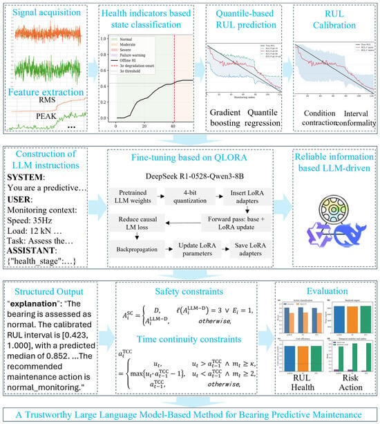
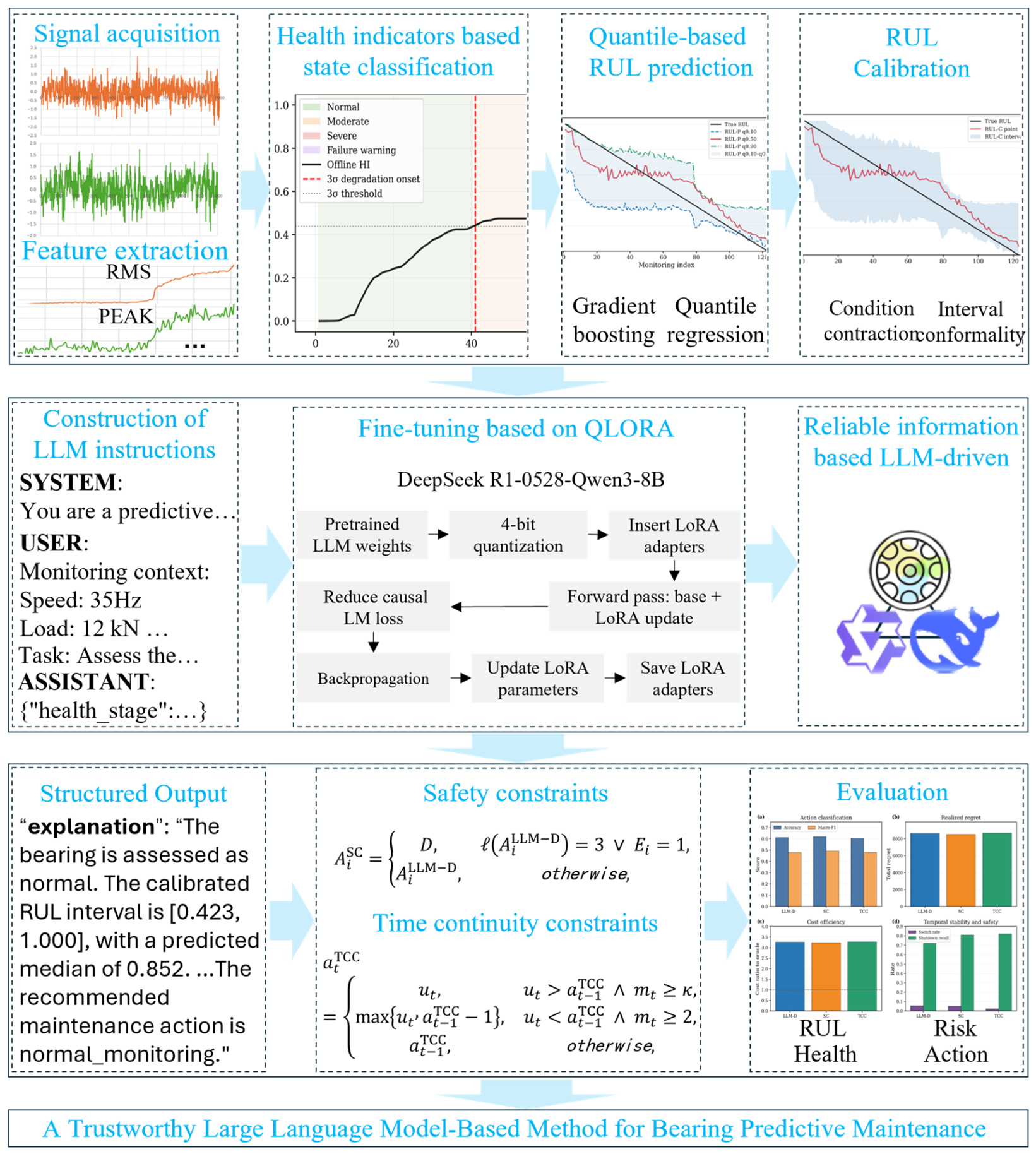
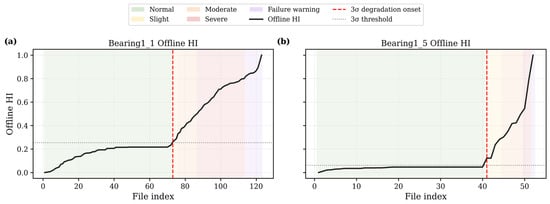
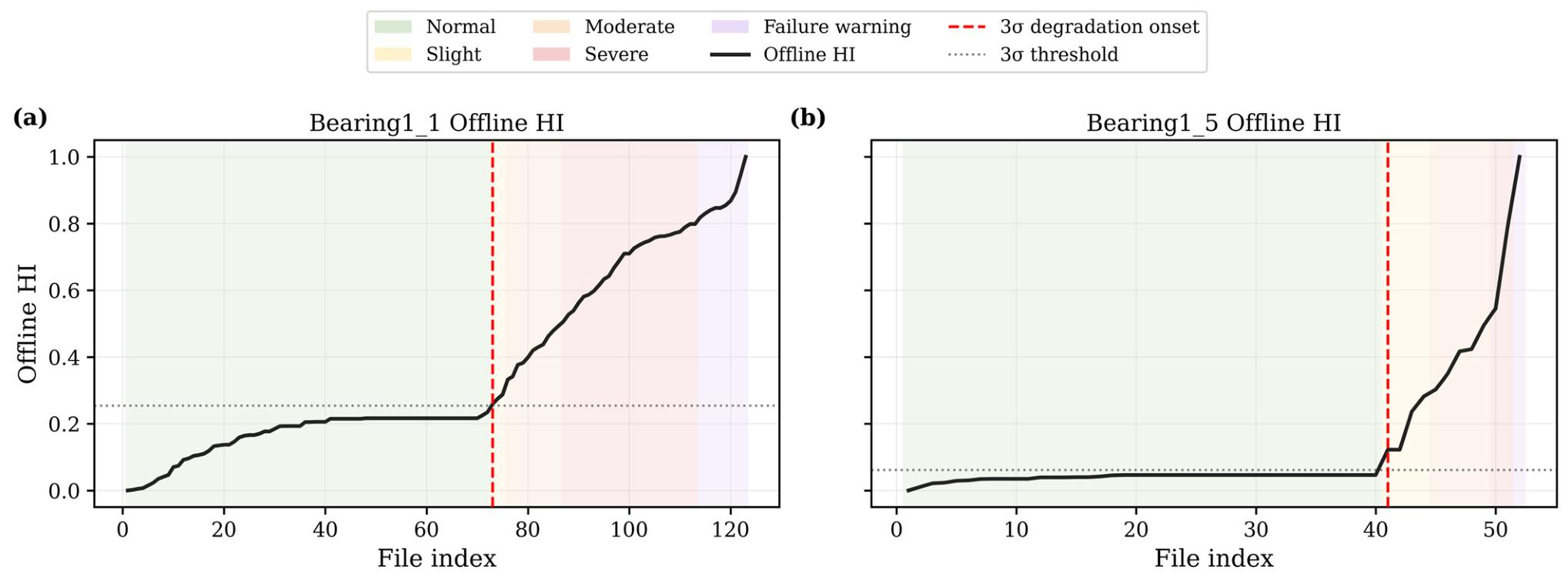
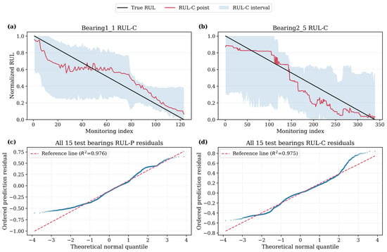
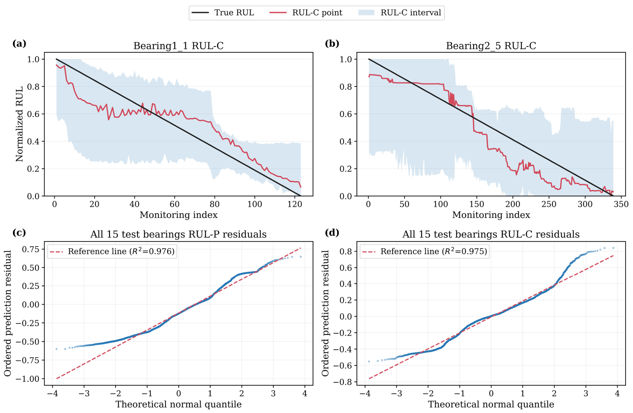
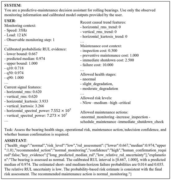
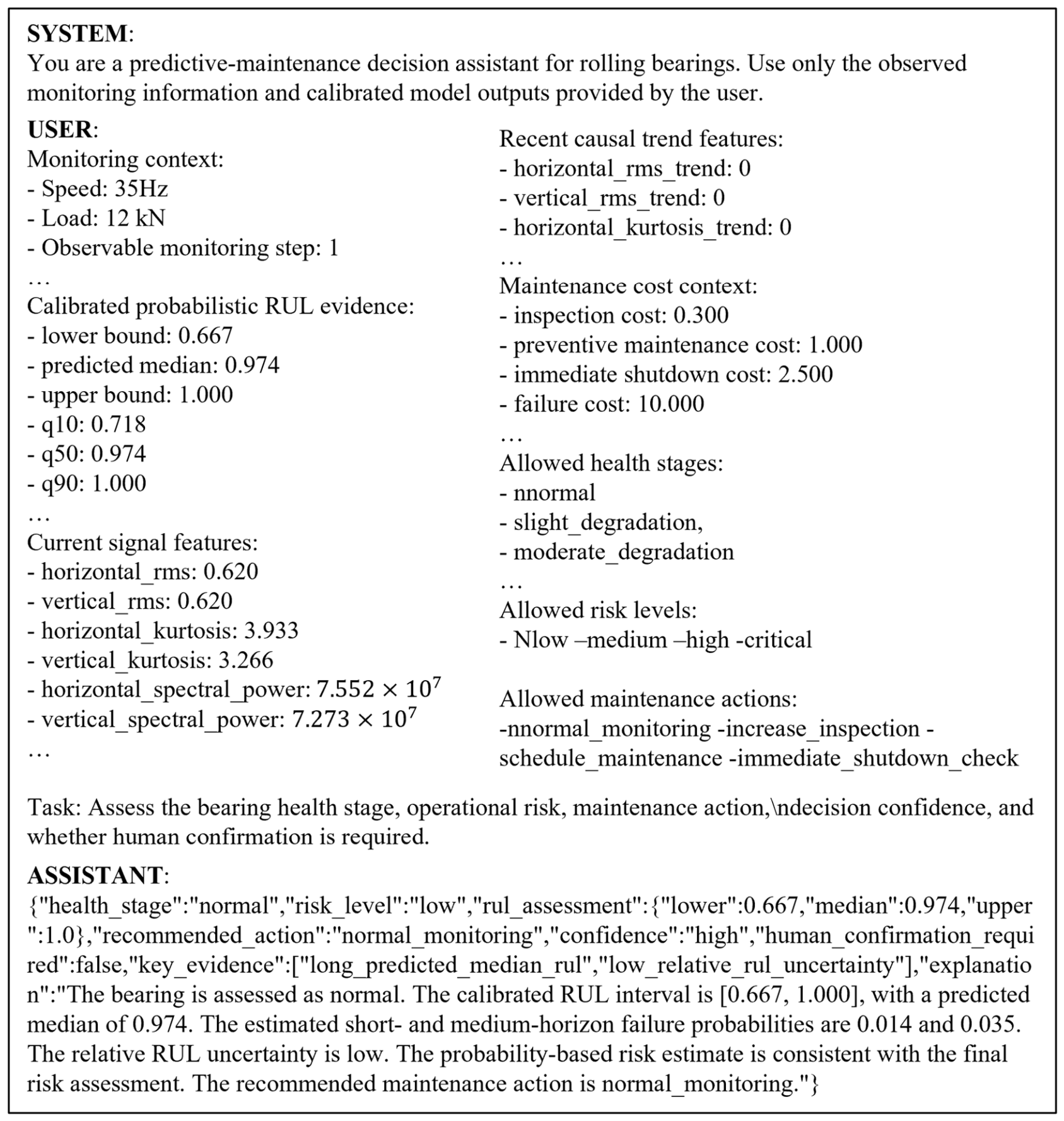
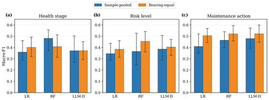
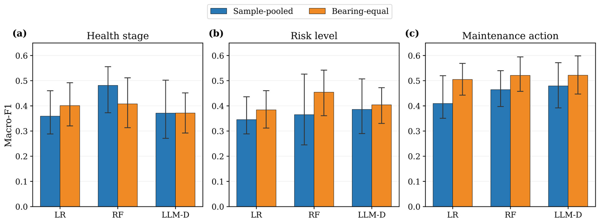
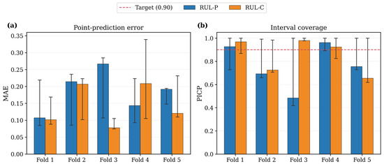
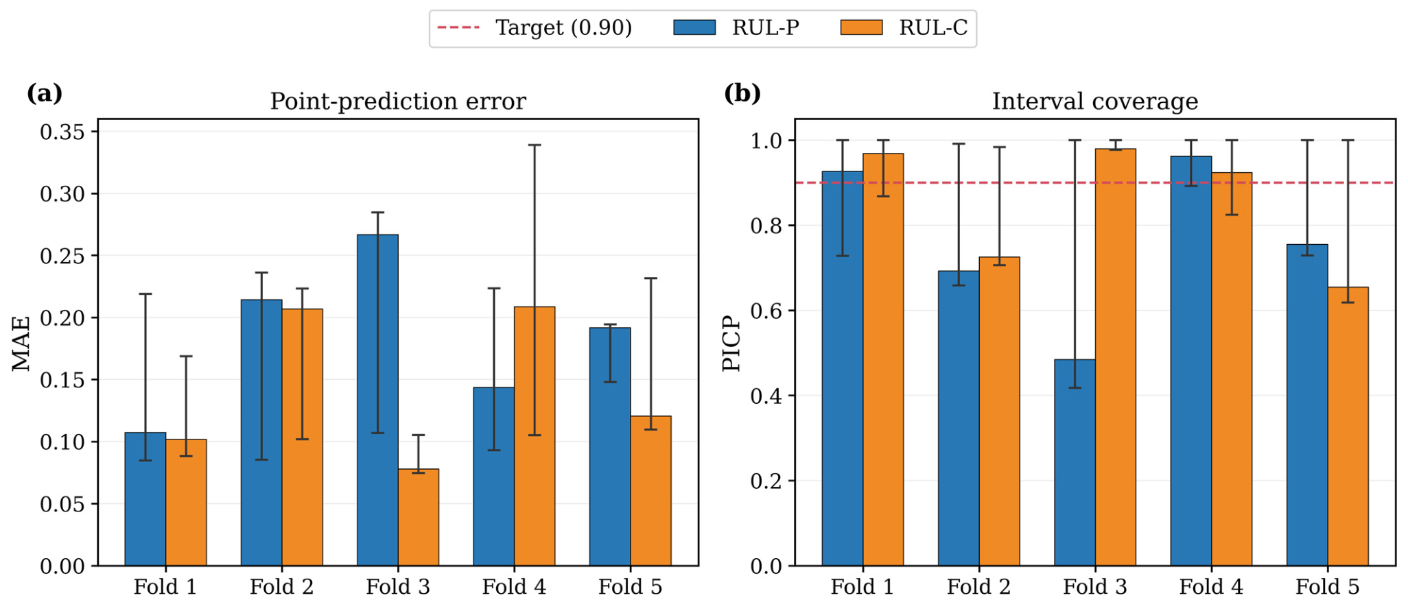
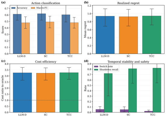
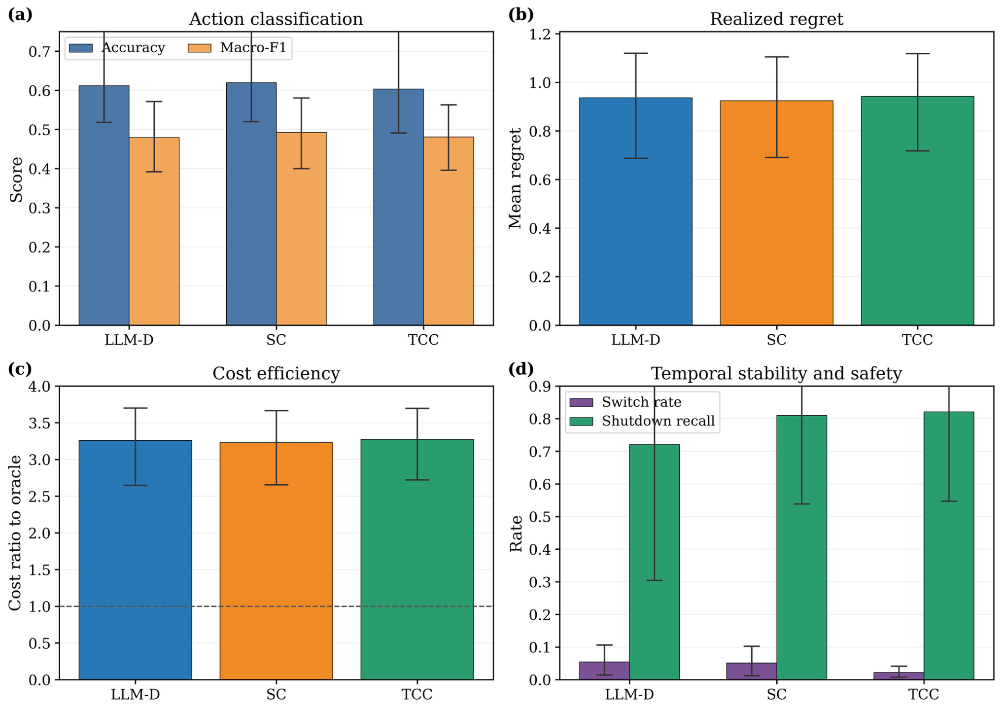
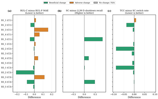
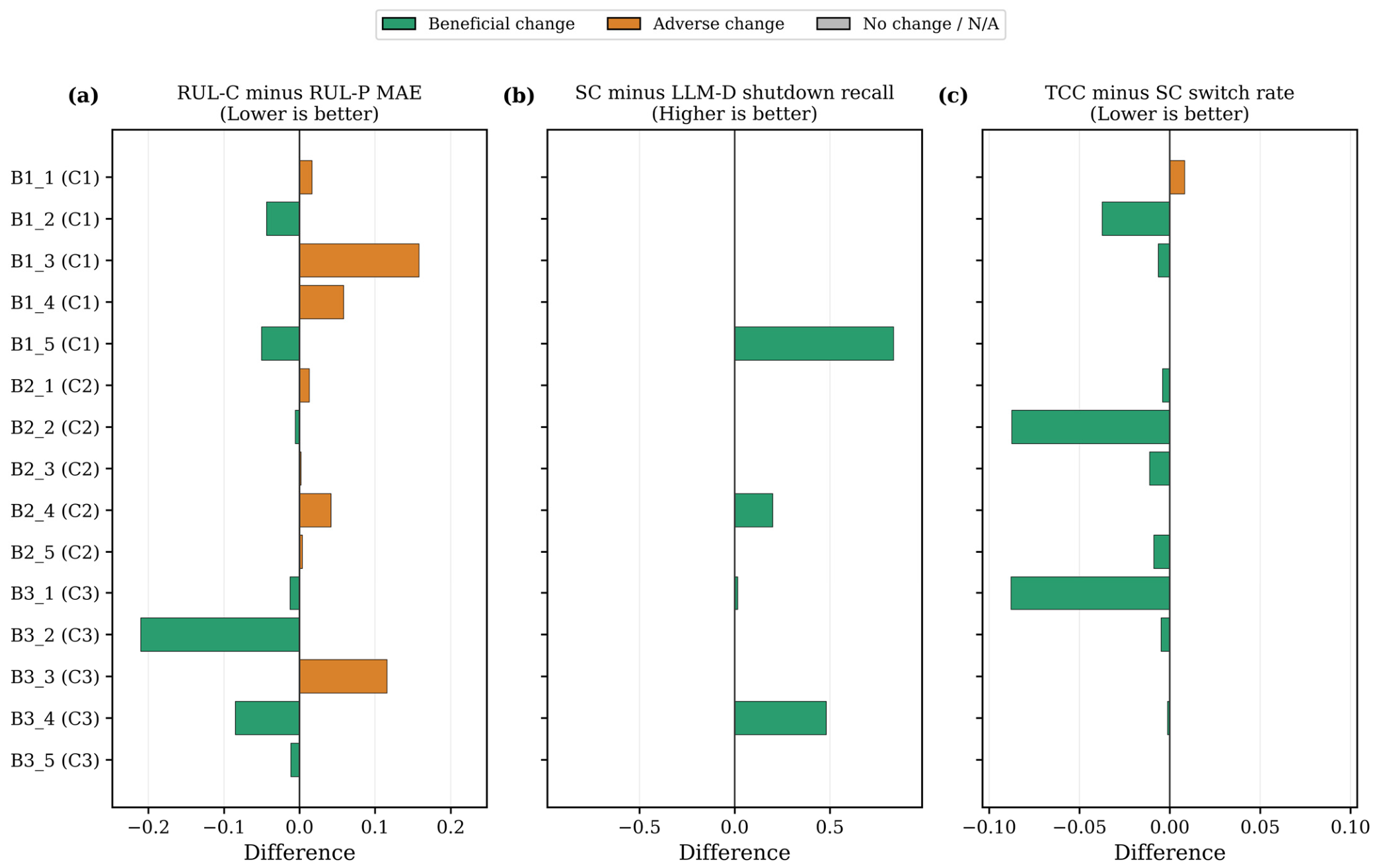
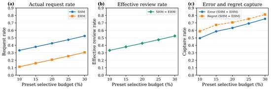
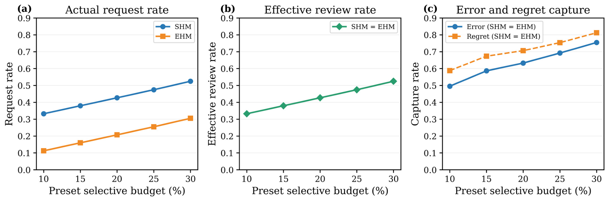

Disclaimer/Publisher’s Note: The statements, opinions and data contained in all publications are solely those of the individual author(s) and contributor(s) and not of MDPI and/or the editor(s). MDPI and/or the editor(s) disclaim responsibility for any injury to people or property resulting from any ideas, methods, instructions or products referred to in the content. |
© 2026 by the authors. Licensee MDPI, Basel, Switzerland. This article is an open access article distributed under the terms and conditions of the Creative Commons Attribution (CC BY) license.