Prediction-Oriented Hankel Matrix Reduction for Data-Driven Predictive Control: Application to Wind Turbine Control

Abstract

Data-driven predictive control methods based on Hankel matrices predict future system behavior directly from measured input–output data without requiring an explicit mathematical model. Their practical application, however, is often limited by the large Hankel matrices needed to achieve satisfactory prediction accuracy, which increase memory requirements and online computational complexity. This paper proposes a prediction-oriented Hankel matrix reduction framework that selects a subset of stored trajectories according to their contribution to the prediction map rather than conventional matrix-based criteria. A direct proof of the constructive part of Willems’ Fundamental Lemma, based only on linearity and time invariance rather than a state-space realization, is first presented, leading to an output-based prediction model that serves as the theoretical foundation of the proposed approach. Three trajectory-selection algorithms with different computational characteristics are then developed to preserve the prediction map while reducing the number of retained Hankel columns. The proposed methods are evaluated through closed-loop control of a nonlinear wind turbine using data-driven predictive control. Simulation results show that substantial reductions in Hankel matrix size can be achieved while maintaining prediction accuracy and comparable closed-loop tracking performance. The proposed framework is structurally applicable to a broad class of Hankel-based data-driven predictive control formulations and can reduce computational complexity while approximately preserving the prediction map.

1. Introduction

Model predictive control (MPC) has become one of the most successful advanced control strategies because of its ability to handle system constraints explicitly, anticipate future events over a moving horizon, accommodate systems with multiple inputs and outputs, and optimize control performance. The performance of conventional MPC, however, strongly depends on the availability of an accurate mathematical model of the controlled system. Developing such a model can require substantial effort and becomes especially difficult when dealing with complex, nonlinear, or time-varying systems. These limitations have motivated the development of data-driven predictive control methods, which make predictions directly from measured input–output trajectories without first identifying an explicit parametric model [1,2,3,4,5].

Among the existing data-driven predictive control approaches, methods based on Hankel matrices constructed from measured trajectories have received considerable attention. These methods exploit behavioral representations of dynamical systems to predict future behavior directly from previously collected data. A major class of data-driven MPC methods is data-enabled predictive control (DeePC), which uses behavioral system theory and Willems’ Fundamental Lemma to represent admissible system trajectories directly from previously collected input–output data and incorporates this representation into a constrained predictive-control optimization problem, without explicitly identifying a parametric model of the system [6,7,8,9]. In DeePC, future input and output trajectories are represented as linear combinations of the columns of Hankel matrices constructed from a persistently exciting input–output trajectory, in accordance with Willems’ Fundamental Lemma [6,7,8,9]. Related Hankel-based prediction mechanisms have also been employed in other data-driven predictive control formulations, including approaches based on segmented trajectories and formulations developed specifically for nonlinear systems [5,10].

A standard deterministic DeePC problem for linear time-invariant (LTI) systems can be formulated at each sampling instant as

$$\begin{array}{cc}\hfill \underset{\mathit{\alpha },{\mathbf{u}}_{\mathrm{future}},{\mathbf{y}}_{\mathrm{future}}}{minimize}& {∥{\mathbf{y}}_{\mathrm{future}}-{\mathbf{y}}_{\mathrm{ref}}∥}_{\mathbf{Q}}^2+{∥{\mathbf{u}}_{\mathrm{future}}∥}_{\mathbf{R}}^2\hfill \\ \hfill \mathrm{subject}\mathrm{to}& \left[\begin{array}{c}{\mathbf{H}}_{u,p}\\ {\mathbf{H}}_{y,p}\\ {\mathbf{H}}_{u,f}\\ {\mathbf{H}}_{y,f}\end{array}\right]\mathit{\alpha }=\left[\begin{array}{c}{\mathbf{u}}_{\mathrm{past}}\\ {\mathbf{y}}_{\mathrm{past}}\\ {\mathbf{u}}_{\mathrm{future}}\\ {\mathbf{y}}_{\mathrm{future}}\end{array}\right],\hfill \\ & {\mathbf{u}}_{\mathrm{future}}\in \mathcal{U},{\mathbf{y}}_{\mathrm{future}}\in \mathcal{Y}.\hfill \end{array}$$

(1)

Here, ${\mathbf{H}}_{u,p}$ and ${\mathbf{H}}_{y,p}$ are Hankel matrices that contain the past portions of the stored input and output trajectories, whereas ${\mathbf{H}}_{u,f}$ and ${\mathbf{H}}_{y,f}$ contain their corresponding future portions. The vectors ${\mathbf{u}}_{\mathrm{past}}$ and ${\mathbf{y}}_{\mathrm{past}}$ contain the most recently measured input and output samples, respectively. The future input and output trajectories are denoted by ${\mathbf{u}}_{\mathrm{future}}$ and ${\mathbf{y}}_{\mathrm{future}}$, and ${\mathbf{y}}_{\mathrm{ref}}$ denotes the reference output trajectory over the prediction horizon. The matrices $\mathbf{Q}$ and $\mathbf{R}$ weight the output-tracking error and control effort, and $\mathcal{U}$ and $\mathcal{Y}$ denote the admissible future-input and future-output sets. The coefficient vector $\mathit{\alpha }$ determines the linear combination of the stored trajectories and therefore has the same dimension as the number of columns of the Hankel matrices.

A major limitation of the formulation presented in (1) is that it is directly applicable only to noise-free LTI systems. When noisy data are used, which is inevitable in practice, there may exist no vector $\mathit{\alpha }$ that satisfies the constraints of the optimization problem, making the problem infeasible. Hence, for noisy data, regularized variants of DeePC incorporating penalties on $\mathit{\alpha }$ or slack variables in the past-trajectory matching constraints, as well as distributionally robust formulations, are employed [7,8,11,12]. Such modifications can improve robustness, reduce overfitting, and affect the bias–variance properties of the resulting predictor [7,8,11,12]. These improvements, however, come at the expense of introducing a bias–variance trade-off and requiring the selection of suitable regularization parameters.

Another limitation of the formulation in (1) is the inclusion of the past input sequence ${\mathbf{u}}_{\mathrm{past}}$. In the output-based prediction framework developed in [13,14], the dynamical condition of the system is represented by a sufficiently long sequence of past outputs, eliminating the explicit use of the past input trajectory. Consequently, a more compact predictive-control formulation can be obtained while retaining the required prediction capability. It should be noted that the trajectory-reduction principle proposed in this paper is not restricted to the output-based formulation considered here and can also be applied to other Hankel-based predictive-control formulations, such as (1), provided that the corresponding prediction map can be explicitly identified.

Regardless of the particular formulation adopted, the prediction capability of Hankel-based methods depends strongly on the richness of the stored trajectory set. A sufficiently informative dataset is required to represent the range of system behaviors relevant to prediction and control. Consequently, practical implementations often employ large collections of measured trajectories, particularly for multiple-input multiple-output (MIMO) systems, long prediction horizons, high sampling frequencies, nonlinear processes, and systems operating under multiple conditions. Recent approaches have further reinforced this tendency by using large collections of historical trajectories to identify or cluster distinct local behaviors of nonlinear processes [15]. Although such large datasets can enrich the behavioral representation, they also increase the size of the corresponding data matrices.

Increasing the size of the stored trajectory set leads to a substantial increase in computational and memory requirements. In formulations such as (1), the dimension of $\mathit{\alpha }$ grows with the number of stored trajectories. As a result, larger Hankel matrices generally lead to larger online optimization problems, more expensive matrix operations, increased memory usage, and longer solution times. These difficulties become particularly important in real-time applications, where the optimization problem must be solved within each sampling interval.

Considerable research effort has therefore been devoted to improving the computational scalability of Hankel-based prediction and control. Existing approaches can be broadly classified into two categories. One category reduces the effective dimension or numerical rank of the data matrices by projecting the original Hankel representation onto a lower-dimensional subspace. An early data-driven predictive control formulation of this type was proposed in [16], where the input–output Hankel matrix was reduced through orthogonal projection and the predictor was constructed in the resulting latent space, thereby reducing the number of manipulated optimization parameters. Related approaches employ low-rank representations based on singular value decomposition (SVD), principal component-type transformations, or CUR factorization [17,18]. SVD-based reduction replaces the original data matrices with a lower-dimensional basis spanning the relevant trajectory subspace under appropriate assumptions [17], whereas CUR-based methods approximate a Hankel matrix using selected rows and columns of the original matrix [18]. An important distinction is that SVD-based reduction represents the data in a new lower-dimensional basis whose basis vectors are generally linear combinations of the measured trajectories, rather than individual measured trajectories. CUR methods retain selected rows and columns of the original matrix, but their objective is primarily matrix approximation. In contrast, the proposed approach retains a subset of the original measured trajectory columns directly, with the subset selected according to its effect on the prediction map.

A second category addresses datasets that are updated online. Recursive and online reduced-order methods update low-dimensional representations as new measurements become available, thereby avoiding the repeated computation of a complete matrix decomposition [19,20]. Other studies reduce online computational complexity by reformulating the predictive-control problem, modifying the predictor architecture, or transferring part of the online computation to an offline learning stage. Equivalent DeePC reformulations can reduce the number of online decision variables while preserving the optimal control solution [21]. Generalized data-driven predictive control combines a least-squares subspace predictor with a Hankel-based predictor, allowing the latter to be constructed from a shorter data sequence [22]. Learning-based approaches have also been proposed in which a deep neural network is trained offline to approximate the DeePC solution mechanism, thereby substantially reducing or, in some implementations, eliminating online optimization [23]. Structure-exploiting approaches use the Hankel or Hankel-like structure of the data matrices to accelerate matrix–vector products and numerical optimization without explicitly eliminating stored trajectories [24]. The effect of Hankel depth and the resulting trajectory-space representation on prediction performance has also been investigated [25]. Although these methods differ substantially in their mathematical formulations and implementations, they generally seek to reduce matrix dimension, numerical rank, memory consumption, or online optimization cost.

The reduction objectives of these methods are usually defined in terms of surrogate measures, such as low-rank approximation error, singular values, matrix conditioning, or computational complexity. Preserving these properties can be highly useful, but it does not directly address the specific input–output relationship implemented by the data-driven predictor. In particular, a small approximation error between the original and reduced Hankel matrices does not necessarily imply that the two predictors produce the same future-output trajectory for the same available measurements and candidate future input.

From the viewpoint of prediction, the ultimate objective is not necessarily to preserve the Hankel matrix itself, but rather to preserve the input–output prediction mapping induced by the original stored trajectory set. For the output-only prediction framework considered in this paper, this mapping can be written as

$${\mathbf{y}}_{\mathrm{future}}=\mathcal{F}\left({\mathbf{y}}_{\mathrm{past}},{\mathbf{u}}_{\mathrm{future}}\right),$$

(2)

where ${\mathbf{y}}_{\mathrm{past}}$ contains the available past output measurements, ${\mathbf{u}}_{\mathrm{future}}$ is a candidate future control trajectory, ${\mathbf{y}}_{\mathrm{future}}$ is the predicted output trajectory, and $\mathcal{F}$ is the mapping. For the conventional DeePC formulation, the corresponding mapping additionally depends on the past input trajectory and may be expressed as

$${\mathbf{y}}_{\mathrm{future}}={\mathcal{F}}_{\mathrm{DeePC}}\left({\mathbf{u}}_{\mathrm{past}},{\mathbf{y}}_{\mathrm{past}},{\mathbf{u}}_{\mathrm{future}}\right).$$

(3)

Preserving the data matrix and preserving the prediction mapping are not equivalent objectives. The contribution of a trajectory column to the prediction cannot be assessed independently, because it depends on how that column interacts with the remaining columns in constructing the predictor. Consequently, two trajectory columns that are close to one another in the data space need not have the same influence on future predictions. Conversely, trajectories that appear substantially different may be interchangeable from the viewpoint of the induced prediction mapping. Therefore, trajectory reduction based only on subspace projection, column similarity, low-rank approximation, or matrix reconstruction error does not directly identify which original trajectories are important for preserving the predictor and may retain trajectories that are redundant from the viewpoint of prediction.

Motivated by this observation, this paper develops a trajectory reduction method that selects a subset of the original Hankel columns according to its ability to preserve the prediction mapping induced by the complete stored trajectory set. Unlike low-rank factorization methods, the proposed approach retains actual measured trajectory columns rather than replacing them with basis vectors formed as linear combinations of the original data. The reduction objective is thus not an approximation of the Hankel matrix itself, but the preservation of the relationship that maps the available measurements and candidate future inputs to the predicted future outputs.

The main contributions of this paper are summarized as follows:

• A direct input–output proof is presented showing that linear combinations of corresponding columns of the input and output Hankel matrices constitute valid trajectories of the same LTI system.
• A prediction-oriented perspective on Hankel trajectory reduction is introduced, showing that the reduction objective should preserve the prediction mapping induced by the original stored trajectory set rather than surrogate matrix properties.
• Three trajectory reduction algorithms with different computational characteristics are proposed based on this principle.
• The effectiveness of the proposed methods is demonstrated on a wind turbine benchmark.

The rest of this paper is organized as follows. Section 2 establishes the theoretical foundation of the proposed method by revisiting the data-driven linear prediction model, presenting a new proof of the constructive part of Willems’ Fundamental Lemma, and deriving the output-based prediction model used throughout the paper. Section 3 formulates the prediction-oriented trajectory reduction problem and proposes three trajectory reduction methods with different computational characteristics. Section 4 demonstrates the effectiveness of the proposed methods through a wind-turbine control case study. Finally, Section 5 concludes the paper with a discussion.

2. Theoretical Development of the Data-Driven Prediction Model

Section 2 revisits the data-driven linear prediction framework from an operator-theoretic perspective to establish the theoretical basis of the proposed trajectory-reduction method. Instead of relying on a state-space realization, the constructive part of Willems’ Fundamental Lemma is derived directly from the fundamental properties of linearity and time invariance. This viewpoint naturally leads to the output-based prediction model that will be used throughout the remainder of the paper.

2.1. Data-Driven Linear Model Revisited

Consider a causal and stable discrete-time LTI system whose input and output trajectories are defined over $\mathbb{Z}$. Let its impulse response be denoted by

$$h={\left\{h\left(i\right)\right\}}_{i\in \mathbb{Z}},$$

(4)

where

$$h\left(i\right)=0,i<0,$$

(5)

as a consequence of causality. The system is also assumed to be stable so that the convolution operator introduced below is well defined on the adopted signal space.

For an input trajectory

$$u={\left\{u\left(k\right)\right\}}_{k\in \mathbb{Z}},$$

(6)

the corresponding output trajectory

$$y={\left\{y\left(k\right)\right\}}_{k\in \mathbb{Z}},$$

(7)

is determined by the convolution relation

$$y\left(k\right)=(h\ast u)\left(k\right)={\displaystyle \sum _{i=0}^{\infty }}h\left(i\right)u(k-i),k\in \mathbb{Z}.$$

(8)

Equation (8) defines a linear mapping from the input trajectory to the output trajectory. We denote this mapping by the convolution operator

$$\mathcal{T}:{𝓁}_2\left(\mathbb{Z}\right)\to {𝓁}_2\left(\mathbb{Z}\right),$$

(9)

whose action is completely characterized by the impulse response (4). Accordingly,

$$y=\mathcal{T}u.$$

(10)

In addition to linearity, the system is time invariant. Let

$$\mathcal{S}:{𝓁}_2\left(\mathbb{Z}\right)\to {𝓁}_2\left(\mathbb{Z}\right),$$

(11)

denote the one-step shift operator defined by

$$\left(\mathcal{S}x\right)\left(k\right)=x(k+1),k\in \mathbb{Z}.$$

(12)

Repeated application of $\mathcal{S}$ generates the shifted trajectories

$$u,\mathcal{S}u,{\mathcal{S}}^{2}u,\dots .$$

(13)

Time invariance implies that shifting an input trajectory before applying it to the system produces the same result as shifting the corresponding output trajectory. Therefore,

$$\mathcal{T}\mathcal{S}=\mathcal{S}\mathcal{T}.$$

(14)

More generally,

$$\mathcal{T}{\mathcal{S}}^i={\mathcal{S}}^i\mathcal{T},i=0,1,2,\dots .$$

(15)

Equation (14) is the operator expression of time invariance and provides the key property used in the following development. In particular, it allows the output associated with any finite linear combination of shifted copies of a known input trajectory to be determined directly from the correspondingly shifted copies of its output trajectory. The following lemma formalizes this observation.

Lemma 1

(Linear combinations of shifted input–output trajectories). Let

$$y_d=\mathcal{T}{u}_d,$$

(16)

be an arbitrary reference input–output trajectory generated by a causal discrete-time LTI system, with $u_d,y_d\in {𝓁}_2\left(\mathbb{Z}\right)$. Let

$$\mathit{\alpha }={\left[\begin{array}{cccc}{\alpha }_0& {\alpha }_1& \cdots & {\alpha }_{N-1}\end{array}\right]}^{\top }\in {\mathbb{R}}^N,$$

(17)

be an arbitrary coefficient vector.

Define the linear operators

$${\mathbf{U}}_s:{\mathbb{R}}^N\to {𝓁}_2\left(\mathbb{Z}\right),{\mathbf{U}}_s\mathit{\alpha }:={\displaystyle \sum _{i=0}^{N-1}}{\alpha }_i{\mathcal{S}}^i{u}_d,$$

(18)

and

$${\mathbf{Y}}_s:{\mathbb{R}}^N\to {𝓁}_2\left(\mathbb{Z}\right),{\mathbf{Y}}_s\mathit{\alpha }:={\displaystyle \sum _{i=0}^{N-1}}{\alpha }_i{\mathcal{S}}^i{y}_d.$$

(19)

Then every input trajectory of the form

$$u={\mathbf{U}}_s\mathit{\alpha }$$

(20)

produces the output

$$y={\mathbf{Y}}_s\mathit{\alpha },$$

(21)

or equivalently,

$$y=\mathcal{T}u.$$

(22)

Proof. 

From (18) and (20),

$$u={\displaystyle \sum _{i=0}^{N-1}}{\alpha }_i{\mathcal{S}}^i{u}_d.$$

(23)

Applying the convolution operator gives

$$\mathcal{T}u=\mathcal{T}\left({\displaystyle \sum _{i=0}^{N-1}}{\alpha }_i{\mathcal{S}}^i{u}_d\right).$$

(24)

Using linearity,

$$\mathcal{T}u={\displaystyle \sum _{i=0}^{N-1}}{\alpha }_i\mathcal{T}{\mathcal{S}}^i{u}_d.$$

(25)

Since the system is time invariant,

$$\mathcal{T}{\mathcal{S}}^i={\mathcal{S}}^i\mathcal{T},i=0,1,\dots ,N-1.$$

(26)

Therefore,

$$\mathcal{T}u={\displaystyle \sum _{i=0}^{N-1}}{\alpha }_i{\mathcal{S}}^i\mathcal{T}{u}_d.$$

(27)

Using (16),

$$\mathcal{T}u={\displaystyle \sum _{i=0}^{N-1}}{\alpha }_i{\mathcal{S}}^i{y}_d.$$

(28)

From the definition of ${\mathbf{Y}}_s$ in (19),

$${\displaystyle \sum _{i=0}^{N-1}}{\alpha }_i{\mathcal{S}}^i{y}_d={\mathbf{Y}}_s\mathit{\alpha }=y.$$

(29)

Hence,

$$y=\mathcal{T}u.$$

(30)

   □

The relations established in Lemma 1 are written for infinite input and output sequences. In practical prediction and control problems, however, only finite-length trajectory segments are used. We therefore restrict the trajectories in (20) and (21) to the indices $k=0,1,\dots ,L-1$. This yields the finite-dimensional representations

$${\mathbf{u}}_L={\mathbf{H}}_u\mathit{\alpha },$$

(31)

and

$${\mathbf{y}}_L={\mathbf{H}}_y\mathit{\alpha },$$

(32)

or equivalently,

$$\left[\begin{array}{c}{\mathbf{u}}_L\\ {\mathbf{y}}_L\end{array}\right]=\left[\begin{array}{c}{\mathbf{H}}_u\\ {\mathbf{H}}_y\end{array}\right]\mathit{\alpha },$$

(33)

where

$${\mathbf{H}}_u=\left[\begin{array}{ccccc}{u}_d\left(0\right)& u_d\left(1\right)& u_d\left(2\right)& \cdots & u_d(N-1)\\ u_d\left(1\right)& u_d\left(2\right)& u_d\left(3\right)& \cdots & u_d\left(N\right)\\ u_d\left(2\right)& u_d\left(3\right)& u_d\left(4\right)& \cdots & u_d(N+1)\\ ⋮& ⋮& ⋮& \ddots & ⋮\\ u_d(L-1)& u_d\left(L\right)& u_d(L+1)& \cdots & u_d(N+L-2)\end{array}\right]\in {\mathbb{R}}^{L\times N},$$

(34)

$${\mathbf{H}}_y=\left[\begin{array}{ccccc}{y}_d\left(0\right)& y_d\left(1\right)& y_d\left(2\right)& \cdots & y_d(N-1)\\ y_d\left(1\right)& y_d\left(2\right)& y_d\left(3\right)& \cdots & y_d\left(N\right)\\ y_d\left(2\right)& y_d\left(3\right)& y_d\left(4\right)& \cdots & y_d(N+1)\\ ⋮& ⋮& ⋮& \ddots & ⋮\\ y_d(L-1)& y_d\left(L\right)& y_d(L+1)& \cdots & y_d(N+L-2)\end{array}\right]\in {\mathbb{R}}^{L\times N},$$

(35)

$${\mathbf{u}}_L={\left[u\left(0\right)u\left(1\right)u\left(2\right)\cdots u(L-1)\right]}^{\top },$$

(36)

$${\mathbf{y}}_L={\left[y\left(0\right)y\left(1\right)y\left(2\right)\cdots y(L-1)\right]}^{\top },$$

(37)

and $\mathit{\alpha }$ is defined in (17).

Thus, the finite-dimensional Hankel representation follows directly from the infinite-dimensional shift-based representation established in Lemma 1. Equation (33) establishes one inclusion underlying Willems’ Fundamental Lemma: every linear combination of corresponding columns of the input and output Hankel matrices is a valid input–output trajectory of the same LTI system. This direction requires only linearity and time invariance and does not require persistent excitation. Under the standard additional assumptions of controllability and persistence of excitation of the required order, the reverse inclusion also holds; namely, every finite-length trajectory of the system admits a representation of the form (33).

2.2. Past–Future Partition for Output-Based Prediction

Assume that the Hankel matrices ${\mathbf{H}}_u$ and ${\mathbf{H}}_y$ are constructed from the reference input–output trajectories $u_d={\left\{u_d\left(k\right)\right\}}_{k=0}^{N+L-2}$ and $y_d={\left\{y_d\left(k\right)\right\}}_{k=0}^{N+L-2}$ according to (34) and (35), respectively. Hence, the vectors ${\mathbf{u}}_L$ and ${\mathbf{y}}_L$ obtained from (31) and (32) are valid vector representations of the trajectories of the system for any coefficient vector $\mathit{\alpha }\in {\mathbb{R}}^N$.

For prediction, however, the future output is not determined by the future input alone. The current dynamical condition of the system, which is specified by a number of past output samples in this paper, must also be considered. Let $L=L_p+L_f$, where $L_p$ and $L_f$ denote the past and future horizons, respectively. It is assumed that $L_p$ is sufficiently large for the measured past output sequence to characterize the current dynamical condition within the adopted output-based prediction framework [13,14]. For a noise-free observable LTI system, a natural guideline is to choose $L_p$ no smaller than the observability index, and therefore a choice $L_p\ge n$ is sufficient when only an upper bound based on the system order n is available.

We partition the output Hankel matrix as

$${\mathbf{H}}_y=\left[\begin{array}{c}{\mathbf{H}}_{y,p}\\ {\mathbf{H}}_{y,f}\end{array}\right],$$

(38)

where ${\mathbf{H}}_{y,p}\in {\mathbb{R}}^{L_p\times N}$ contains the past output segments and ${\mathbf{H}}_{y,f}\in {\mathbb{R}}^{L_f\times N}$ contains the corresponding future output segments. Similarly, the input Hankel matrix is partitioned as

$${\mathbf{H}}_u=\left[\begin{array}{c}{\mathbf{H}}_{u,p}\\ {\mathbf{H}}_{u,f}\end{array}\right],$$

(39)

where ${\mathbf{H}}_{u,p}\in {\mathbb{R}}^{L_p\times N}$ and ${\mathbf{H}}_{u,f}\in {\mathbb{R}}^{L_f\times N}$. Although ${\mathbf{H}}_{u,p}$ is included in the partition for completeness, it is not used in the output-based predictor considered here.

In the proposed prediction framework, the measured recent output sequence ${\mathbf{y}}_{\mathrm{past}}$ is matched to the past-output block through

$${\mathbf{H}}_{y,p}\mathit{\alpha }={\mathbf{y}}_{\mathrm{past}}.$$

(40)

The future input sequence to be applied to the system is imposed through

$${\mathbf{H}}_{u,f}\mathit{\alpha }={\mathbf{u}}_{\mathrm{future}}.$$

(41)

Once a coefficient vector $\mathit{\alpha }$ satisfying (40) and (41) is found, the corresponding future output prediction is obtained as

$${\mathbf{y}}_{\mathrm{future}}={\mathbf{H}}_{y,f}\mathit{\alpha }.$$

(42)

3. Prediction-Oriented Reduction of the Stored Trajectory Set

Based on the discussion in the previous section, to predict the system response to the input vector ${\mathbf{u}}_{\mathrm{future}}$, assuming that the vector ${\mathbf{y}}_{\mathrm{past}}$ contains a sufficient number of the most recent consecutive samples of the system output, we compute the vector $\mathit{\alpha }$ from the following equation:

$$\left[\begin{array}{c}{\mathbf{H}}_{y,p}\\ {\mathbf{H}}_{u,f}\end{array}\right]\mathit{\alpha }=\left[\begin{array}{c}{\mathbf{y}}_{\mathrm{past}}\\ {\mathbf{u}}_{\mathrm{future}}\end{array}\right].$$

(43)

Then, using the obtained value of $\mathit{\alpha }$, the vector ${\mathbf{y}}_{\mathrm{future}}$ containing the predicted output trajectory is computed from (42). To establish an explicit relationship among the future input vector, the past output vector, and the future output vector, we must eliminate the intermediate variable $\mathit{\alpha }$ from these equations. The minimum-norm solution of (43) is given by

$$\mathit{\alpha }={\left[\begin{array}{c}{\mathbf{H}}_{y,p}\\ {\mathbf{H}}_{u,f}\end{array}\right]}^{†}\left[\begin{array}{c}{\mathbf{y}}_{\mathrm{past}}\\ {\mathbf{u}}_{\mathrm{future}}\end{array}\right].$$

(44)

Now, by substituting $\mathit{\alpha }$ from (44) into (42), we obtain the direct prediction map from past outputs and future inputs to future outputs:

$${\mathbf{y}}_{\mathrm{future}}={\mathbf{H}}_{y,f}{\left[\begin{array}{c}{\mathbf{H}}_{y,p}\\ {\mathbf{H}}_{u,f}\end{array}\right]}^{†}\left[\begin{array}{c}{\mathbf{y}}_{\mathrm{past}}\\ {\mathbf{u}}_{\mathrm{future}}\end{array}\right].$$

(45)

The above equation clearly shows how the future input trajectory and the past output trajectory jointly influence the future output trajectory.

Note that since in practice $L\ll N$, (43) is underdetermined and generally has infinitely many solutions for $\mathit{\alpha }$. However, all such $\mathit{\alpha }$ vectors yield the same future-output prediction in the exact deterministic LTI setting considered here. This is because a sufficiently long past-output trajectory specifies the current dynamical condition of the system, and the prescribed future-input trajectory then uniquely determines the corresponding future-output trajectory. Therefore, in the above discussion, since all solutions of (43) yield the same future-output prediction in the exact deterministic LTI setting, we used one such $\mathit{\alpha }$, obtained from (44), for this purpose.

Note also that (45) can be directly extended to the conventional DeePC setting in (1), for which the prediction mapping in (3) also depends on the past input trajectory. In this case, in addition to (40) and (41), the coefficient vector $\mathit{\alpha }$ satisfies

$${\mathbf{H}}_{u,p}\mathit{\alpha }={\mathbf{u}}_{\mathrm{past}}.$$

(46)

Following calculations analogous to those in (43)–(45), the future-output prediction can then be written as

$${\mathbf{y}}_{\mathrm{future}}={\mathbf{H}}_{y,f}{\left[\begin{array}{c}{\mathbf{H}}_{u,p}\\ {\mathbf{H}}_{y,p}\\ {\mathbf{H}}_{u,f}\end{array}\right]}^{†}\left[\begin{array}{c}{\mathbf{u}}_{\mathrm{past}}\\ {\mathbf{y}}_{\mathrm{past}}\\ {\mathbf{u}}_{\mathrm{future}}\end{array}\right].$$

(47)

Equation (45) (or (47) for DeePC) provides a framework for eliminating redundant columns from the matrices ${\mathbf{H}}_u$ and ${\mathbf{H}}_y$, thereby yielding a reduced-size data-driven predictor. At first glance, it may seem that those columns of ${\mathbf{H}}_y$ or ${\mathbf{H}}_u$ that are highly similar to one another (where similarity is measured by a small norm of the difference between the corresponding columns) have nearly identical effects on the prediction of the system output, and therefore that some of them can be safely eliminated. However, (45) shows that the future output trajectory is predicted using the matrix

$$\mathbf{M}:={\mathbf{H}}_{y,f}{\left[\begin{array}{c}{\mathbf{H}}_{y,p}\\ {\mathbf{H}}_{u,f}\end{array}\right]}^{†}.$$

(48)

Therefore, the decision regarding which columns should be removed from ${\mathbf{H}}_y$ and ${\mathbf{H}}_u$ should be based on their impact on this matrix.

Suppose we retain a subset of the columns of ${\mathbf{H}}_y$ and ${\mathbf{H}}_u$, indexed by $\mathcal{S}$ ($\mathcal{S}\subseteq \{1,\dots ,N\}$), and remove the remaining columns. Accordingly, ${\mathbf{H}}_y^{\mathcal{S}}$ and ${\mathbf{H}}_u^{\mathcal{S}}$ denote the reduced matrices obtained after deleting the unselected columns of ${\mathbf{H}}_y$ and ${\mathbf{H}}_u$, respectively. Using these notations, the mapping from ${\mathbf{y}}_{\mathrm{past}}$ and ${\mathbf{u}}_{\mathrm{future}}$ to ${\mathbf{y}}_{\mathrm{future}}$ can be expressed in terms of the reduced matrices as follows:

$${\mathbf{M}}_{\mathcal{S}}:={\mathbf{H}}_{y,f}^{\mathcal{S}}{\left[\begin{array}{c}{\mathbf{H}}_{y,p}^{\mathcal{S}}\\ {\mathbf{H}}_{u,f}^{\mathcal{S}}\end{array}\right]}^{†}.$$

(49)

Note that since $L=L_p+L_f$, both the original and reduced prediction maps have dimensions $M,M_{\mathcal{S}}\in {\mathbb{R}}^{L_f\times L}$.

According to the above discussion, the problem of column elimination can be formulated as finding the index set $\mathcal{S}$ such that a norm of $\mathbf{M}-{\mathbf{M}}_{\mathcal{S}}$ is minimized. This problem can, for example, be formulated as the following constrained optimization problem:

$$\begin{array}{cc}\hfill \underset{\mathcal{S}}{minimize}& \left|\mathcal{S}\right|\hfill \end{array}$$

(50a)

$$\begin{array}{cc}\hfill \mathrm{subject}\mathrm{to}& {\displaystyle \frac{{∥\mathbf{M}-{\mathbf{M}}_{\mathcal{S}}∥}_2}{{∥\mathbf{M}∥}_2}}\le \epsilon ,\hfill \end{array}$$

(50b)

where $\epsilon >0$ is the maximum admissible relative prediction-map error, ${\parallel ·\parallel }_2$ denotes the induced 2-norm, and $\left|\mathcal{S}\right|$ is the cardinality of the retained column set. For any nonzero stacked input vector

$$\mathbf{b}=\left[\begin{array}{c}{\mathbf{y}}_{\mathrm{past}}\\ {\mathbf{u}}_{\mathrm{future}}\end{array}\right],$$

(51)

the discrepancy between the predictions generated by the full and reduced maps satisfies

$${\displaystyle \frac{{∥(\mathbf{M}-{\mathbf{M}}_S)\mathbf{b}∥}_2}{{\parallel \mathbf{M}\parallel }_2{\parallel \mathbf{b}\parallel }_2}}\le {\displaystyle \frac{\parallel \mathbf{M}-{\mathbf{M}}_S{\parallel }_2}{{\parallel \mathbf{M}\parallel }_2}}\le \epsilon .$$

(52)

Therefore, $\epsilon$ provides a uniform upper bound on the prediction discrepancy relative to the worst-case output magnitude ${\parallel \mathbf{M}\parallel }_2{\parallel \mathbf{b}\parallel }_2$ associated with an input of norm ${\parallel \mathbf{b}\parallel }_2$. It should be noted that this normalization is not, in general, equal to normalization by the particular full-map prediction ${\parallel \mathbf{Mb}\parallel }_2$.

Note that if we apply the column-elimination approach described above to the DeePC problem in (1), the problem will still be formulated as given in (50), with the difference that, according to (47), the matrix $\mathbf{M}$ must be defined as follows:

$${\mathbf{M}}_{\mathrm{DeePC}}:={\mathbf{H}}_{y,f}{\left[\begin{array}{c}{\mathbf{H}}_{u,p}\\ {\mathbf{H}}_{y,p}\\ {\mathbf{H}}_{u,f}\end{array}\right]}^{†},$$

(53)

and the matrix ${\mathbf{M}}_S$ be defined accordingly. Thus, including the past input changes the data matrix entering the prediction map but does not change the prediction-oriented reduction principle developed above. In the remainder of the paper, we proceed with the discussion assuming that the system output is predicted using (45) and that the matrices $\mathbf{M}$ and ${\mathbf{M}}_S$ are defined according to (48) and (49), respectively.

3.1. Approximate Prediction-Map-Preserving Reduction Methods

The exact solution of the subset-selection problem in (50) is combinatorial. If the original Hankel data matrices contain N columns, the number of possible nonempty column subsets is $2^N-1$. Consequently, exhaustive evaluation becomes impractical even for a moderately large trajectory set. In the following, three (approximate) strategies are considered to find $\mathcal{S}$. These methods provide different compromises between computational cost and direct preservation of the prediction capability.

Let

$$\mathbf{G}:=\left[\begin{array}{c}{\mathbf{H}}_{y,p}\\ {\mathbf{H}}_{u,f}\end{array}\right],\mathbf{O}:={\mathbf{H}}_{y,f},$$

(54)

and define the prediction map associated with the full trajectory set as

$$\mathbf{M}:=\mathbf{O}{\mathbf{G}}^{†}.$$

(55)

For a subset of retained column indices $\mathcal{S}\subseteq \{1,\dots ,N\}$, define

$${\mathbf{G}}_{\mathcal{S}}:=\mathbf{G}(:,\mathcal{S}),{\mathbf{O}}_{\mathcal{S}}:=\mathbf{O}(:,\mathcal{S}),$$

(56)

and

$${\mathbf{M}}_{\mathcal{S}}:={\mathbf{O}}_{\mathcal{S}}{\mathbf{G}}_{\mathcal{S}}^{†}.$$

(57)

The following three approximate methods are proposed for selecting $\mathcal{S}$.

3.1.1. Method 1: Greedy Trajectory Elimination

The first method removes one column at a time. At a given iteration, let $\mathcal{S}$ denote the current set of retained columns. For every $j\in \mathcal{S}$, the prediction-map error that would result from deleting column j is evaluated as

$$J_j^{\left(\mathcal{S}\right)}={∥\mathbf{M}-{\mathbf{M}}_{\mathcal{S}\setminus \left\{j\right\}}∥}_2.$$

(58)

The column producing the smallest prediction-map error is selected for removal:

$$j^{\star }=\underset{j\in \mathcal{S}}{arg\; min}{J}_j^{\left(\mathcal{S}\right)}.$$

(59)

The elimination is accepted if

$${\displaystyle \frac{{∥\mathbf{M}-{\mathbf{M}}_{\mathcal{S}\setminus \left\{j^{\star }\right\}}∥}_2}{{∥\mathbf{M}∥}_2}}\le \epsilon ,$$

(60)

where $\epsilon$ is the maximum admissible relative prediction-map error. The retained set is then updated according to

$$\mathcal{S}\leftarrow \mathcal{S}\setminus \left\{j^{\star }\right\},$$

(61)

and the procedure is repeated until no additional column can be deleted without violating (60).

This method directly approximates the original subset-selection problem. However, it requires repeated computation of reduced prediction maps and is therefore computationally demanding for Hankel matrices with a large number of columns.

3.1.2. Method 2: Importance-Based Trajectory Ranking

Unlike the greedy elimination strategy, which repeatedly searches for the least influential column after every elimination, the second method first evaluates the importance of every trajectory column only once using the original Hankel matrices. The columns are then ranked according to their individual contributions to the prediction map, and the resulting ranking is kept fixed throughout the reduction process.

For the matrix $\mathbf{M}$ defined in (55), the importance of the jth column is quantified by evaluating the change in the prediction map after removing only that column while keeping all other columns unchanged. Specifically, let $G_{\{-j\}}$ and $O_{\{-j\}}$ denote the matrices obtained by removing the jth corresponding trajectory column from G and O, respectively, and define

$$M_{\{-j\}}:=O_{\{-j\}}{G}_{\{-j\}}^{†}.$$

(62)

Thus, $M_{\{-j\}}$ has the same dimensions as M. Then the corresponding importance score is defined as

$$I_j={\displaystyle \frac{{∥\mathbf{M}-{\mathbf{M}}_{\{-j\}}∥}_2}{{∥\mathbf{M}∥}_2}}.$$

(63)

A small value of $I_j$ indicates that the corresponding trajectory has little influence on the prediction map and is therefore a good candidate for removal.

After the importance scores have been computed, they are sorted in ascending order. Let $S_r$ denote the set of retained columns after the first r columns in the fixed ranking have been removed. The cumulative relative prediction-map error at this stage is defined as

$$e_r:={\displaystyle \frac{\parallel \mathbf{M}-{\mathbf{M}}_{S_r}{\parallel }_2}{{\parallel \mathbf{M}\parallel }_2}}.$$

(64)

The rth deletion is accepted only if

$$e_r\le \epsilon ,$$

(65)

where $\epsilon$ is the prescribed maximum admissible relative prediction-map error.

Compared with the greedy method, the importance scores are computed only once and no re-ranking is performed after subsequent eliminations. Consequently, the computational burden associated with repeated column searches is significantly reduced while the cumulative prediction-map error is still controlled by the prescribed tolerance.

3.1.3. Method 3: Similarity-Guided, Prediction-Validated Trajectory Pruning

The first two methods evaluate the influence of every trajectory column on the prediction map, either sequentially or through an importance ranking. Although these approaches usually produce accurate reduced trajectory sets, they require repeated construction of reduced prediction maps and therefore become computationally expensive for large Hankel matrices.

The third method adopts a different strategy. Instead of evaluating every column individually, it first identifies only those trajectory columns that are likely to be redundant. This preliminary screening is performed using inexpensive pairwise similarity measures, while the prediction-map error is used only as a validation criterion. Consequently, the expensive prediction-map evaluation is carried out only for the screened candidate columns.

Let ${\mathbf{g}}_i$ and ${\mathbf{g}}_j$ denote the ith and jth columns of the matrix $\mathbf{G}$, and let ${\mathbf{o}}_i$ and ${\mathbf{o}}_j$ denote the corresponding columns of $\mathbf{O}$. Their normalized distances are defined as

$$d_G(i,j)={\displaystyle \frac{\parallel {\mathbf{g}}_i-{\mathbf{g}}_j{\parallel }_2}{\parallel {\mathbf{g}}_i{\parallel }_2}},$$

(66)

and

$$d_O(i,j)={\displaystyle \frac{\parallel {\mathbf{o}}_i-{\mathbf{o}}_j{\parallel }_2}{\parallel {\mathbf{o}}_i{\parallel }_2}}.$$

(67)

If

$$d_G(i,j)\le {\epsilon }_G,d_O(i,j)\le {\epsilon }_O,$$

(68)

the two trajectory columns are regarded as a potentially redundant pair, and column j is selected as a candidate for removal.

The similarity measures alone do not guarantee preservation of the prediction map. Therefore, before permanently removing the candidate column, the corresponding reduced prediction map is recomputed and its relative error is evaluated according to

$${\displaystyle \frac{\parallel \mathbf{M}-{\mathbf{M}}_S{\parallel }_2}{{\parallel \mathbf{M}\parallel }_2}}\le \epsilon .$$

(69)

The candidate column is removed only if the above condition is satisfied; otherwise it is retained. The procedure is repeated until all candidate pairs have been examined.

The rationale behind this method is that trajectory columns exhibiting similar predictor and prediction vectors are more likely to contain redundant information. Consequently, they provide good candidates for removal, while the final decision is made exclusively according to the prediction-map error, thereby controlling the deviation of the reduced prediction map from the full one.

In practice, ${\epsilon }_G$ and ${\epsilon }_O$ in (68) may be selected as moderate screening thresholds and adjusted to control the number of candidate pairs. These parameters affect computational effort rather than the final admissible prediction-map error, since every accepted deletion must still satisfy the prescribed tolerance $\epsilon$.

3.1.4. Computational Complexity

The dominant computational operation in the three reduction methods is the evaluation of a reduced prediction map $M_{\mathcal{S}}=O_{\mathcal{S}}{G}_{\mathcal{S}}^{†}$. Let N denote the number of columns in the original Hankel matrices and L the number of rows of G. For an $L\times n$ matrix with $n\ge L$, an SVD-based pseudoinverse has a computational complexity of $\mathcal{O}\left(n{L}^2\right)$ [26]. This result can be used to estimate the dominant complexity of the three proposed methods.

In Method 1, when n columns remain, the effect of deleting each of the n columns is evaluated separately. Thus, approximately n pseudoinverses, each with complexity $\mathcal{O}\left(n{L}^2\right)$, are required at that elimination step. In the worst case, repeating this process over successive eliminations gives

$${\displaystyle \sum _{n=1}^N}\mathcal{O}\left(n^2{L}^2\right)=\mathcal{O}\left(N^3{L}^2\right).$$

(70)

This is a worst-case complexity estimate; in practice, the algorithm terminates once no additional column can be removed without violating the prescribed prediction-map error tolerance and may therefore require substantially fewer evaluations. The repeated re-evaluation of the remaining columns nevertheless explains the relatively high offline cost of Method 1.

Method 2 computes the individual importance scores for all N columns only once. This requires N leave-one-out prediction-map evaluations and therefore $\mathcal{O}\left(N^2{L}^2\right)$ operations. Sorting the resulting scores requires $\mathcal{O}(NlogN)$ operations. Subsequent cumulative-error checks require at most $\mathcal{O}\left(N\right)$ additional prediction-map evaluations and hence do not change the dominant order. Therefore, the overall dominant complexity of Method 2 is $\mathcal{O}\left(N^2{L}^2\right)$.

Method 3 first screens pairs of trajectory columns using the distances in (66)–(68). There are $N(N-1)/2=\mathcal{O}\left(N^2\right)$ possible column pairs. For each pair, computing $d_G(i,j)$ involves vectors in ${\mathbb{R}}^L$, whereas computing $d_O(i,j)$ involves vectors in ${\mathbb{R}}^{L_f}$. Since $L_f\le L$, the computational cost of the two distance calculations for each pair is $\mathcal{O}\left(L\right)$. Consequently, the overall pairwise screening cost is $\mathcal{O}\left(N^{2}L\right)$. Let K denote the number of screened candidates for which a prediction-map evaluation is subsequently required. These evaluations have a total cost of approximately $\mathcal{O}\left(KN{L}^2\right)$, giving

$$\mathcal{O}(N^{2}L+KN{L}^2)$$

(71)

for Method 3. The value of K depends on the similarity thresholds and the data; when the screening eliminates most pairs from further consideration, K is substantially smaller than the total number of possible pairs. These complexity estimates are consistent with the measured offline computation times reported in Table 1.

Table 1. Computational comparison of the full and reduced Hankel formulations.

Method	Columns	Red. (%)	Error (%)	Memory (MB)	Offline (s)	QP (ms)
Full	961	0.0	0	1.173	0	490.3
Method 1	458	52.3	1.016	0.559	921.7	80.2
Method 2	801	16.6	0.961	0.978	4.35	317.1
Method 3	633	34.1	0.995	0.773	12.0	151.9

4. Application to Wind Turbine Control

To evaluate the effectiveness of the proposed reduced-size data-driven predictive control method, it is applied to a variable-speed horizontal-axis wind turbine. Wind-turbine control provides a suitable case study because the aerodynamic dynamics are nonlinear and the available wind power continuously varies with the wind speed. The control objective considered in this section is to extract a large amount of electrical power while maintaining the turbine near an aerodynamically efficient operating condition.

A widely used nonlinear dynamic model of a variable-speed horizontal-axis wind turbine is adopted in this paper [27]. The model contains two state variables: the rotor angular speed and the generator torque. The blade pitch angle and the load-switching duty cycle are considered as the control inputs, whereas the tip-speed ratio and the generated electrical power are selected as the measured outputs. The nonlinear model described below is used only to generate the input–output data and to simulate the plant. For the nonlinear plant considered here, the Hankel-based predictor is used as a finite-data approximation, and the exact LTI trajectory representation established in Section 2 is not claimed to hold globally.

The dynamics of the turbine are described by

$$\begin{array}{cc}\hfill J\dot{\omega }\left(t\right)& =T_a\left(t\right)-T_g\left(t\right)-B\omega \left(t\right),\hfill \end{array}$$

(72)

$$\begin{array}{cc}\hfill {\tau }_g{\dot{T}}_g\left(t\right)& =K_{d}d\left(t\right)-T_g\left(t\right),\hfill \end{array}$$

(73)

where $\omega$ is the rotor angular speed, $T_g$ is the generator torque, J is the equivalent rotational inertia, B is the viscous-friction coefficient, ${\tau }_g$ is the generator time constant, $K_d$ is the gain relating the duty cycle to generator torque, and d is the load-switching duty cycle.

The aerodynamic torque is obtained from

$$T_a\left(t\right)={\displaystyle \frac{P_a\left(t\right)}{\omega \left(t\right)}},$$

(74)

where the aerodynamic power extracted from the wind is

$$P_a\left(t\right)={\displaystyle \frac{1}{2}}\rho A{V}_w^3\left(t\right)C_p\left(\lambda \left(t\right),\beta \left(t\right)\right).$$

(75)

Here, $\rho$ is the air density, $A=\pi R^2$ is the rotor swept area, R is the rotor radius, $V_w$ is the wind speed, and $\beta$ is the blade pitch angle. The tip-speed ratio is defined as

$$\lambda \left(t\right)={\displaystyle \frac{R\omega \left(t\right)}{V_w\left(t\right)}}.$$

(76)

In (75) the following widely adopted empirical approximation of the power coefficient, $C_p\left(\lambda \left(t\right),\beta \left(t\right)\right)$, is employed [27,28]:

$$C_p(\lambda ,\beta )=c_1\left({\displaystyle \frac{c_2}{{\lambda }_i}}-c_3\beta -c_4\right)exp\left(-{\displaystyle \frac{c_5}{{\lambda }_i}}\right)+c_6\lambda ,$$

(77)

where

$${\displaystyle \frac{1}{{\lambda }_i}}={\displaystyle \frac{1}{\lambda +0.08\beta }}-{\displaystyle \frac{0.035}{{\beta }^3+1}},$$

(78)

and

$$c_1=0.5176,c_2=116,c_3=0.4,c_4=5,c_5=21,c_6=0.0068.$$

(79)

For the adopted aerodynamic model, the maximum of $C_p(\lambda ,\beta )$ occurs approximately at

$${\beta }_{\mathrm{opt}}=0^{\circ },{\lambda }_{\mathrm{opt}}\simeq 8.1.$$

(80)

The generated electrical power is calculated as

$$P_e\left(t\right)={\eta }_g{T}_g\left(t\right)\omega \left(t\right),$$

(81)

where ${\eta }_g$ denotes the generator efficiency. For numerical implementation, a sufficiently small positive constant ${\epsilon }_0$ may be added to the denominator of (74) to prevent division by zero at very low rotor speeds.

The parameters used in the simulations are selected as $\rho =1.225\mathrm{kg}/{\mathrm{m}}^3$, $R=1.5\mathrm{m}$, $A=\pi R^2=7.07{\mathrm{m}}^2$, $J=8\mathrm{kg}{\mathrm{m}}^2$, $B=0.02\mathrm{N}\mathrm{m}\mathrm{s}/\mathrm{rad}$, ${\tau }_g=0.15\mathrm{s}$, $K_d=25\mathrm{N}\mathrm{m}$, ${\eta }_g=0.85$, and ${\epsilon }_0={10}^{-3}\mathrm{rad}/\mathrm{s}$. These values describe a small variable-speed wind turbine and provide a nonlinear simulation benchmark for evaluating the proposed controller.

4.1. Control Problem Formulation

The wind turbine is treated as a two-input two-output system whose input and output vectors are defined as

$$\mathbf{u}\left(k\right)=\left[\begin{array}{c}\beta \left(k\right)\\ d\left(k\right)\end{array}\right],\mathit{y}\left(k\right)=\left[\begin{array}{c}\lambda \left(k\right)\\ P_e\left(k\right)\end{array}\right].$$

(82)

Thus, the controller determines the blade pitch angle and the load-switching duty cycle, whereas the measured outputs are the tip-speed ratio and the generated electrical power.

Let the input–output data collected from the nonlinear wind-turbine model be denoted by

$${\left\{{\beta }_{\mathrm{d}}\left(k\right),d_{\mathrm{d}}\left(k\right),{\lambda }_{\mathrm{d}}\left(k\right),P_{e,\mathrm{d}}\left(k\right)\right\}}_{k=0}^{N+L-2}.$$

(83)

The corresponding Hankel matrices are denoted by

$${\mathbf{H}}_{\beta },{\mathbf{H}}_d,{\mathbf{H}}_{\lambda },{\mathbf{H}}_P,$$

(84)

where ${\mathbf{H}}_{\beta },{\mathbf{H}}_d,{\mathbf{H}}_{\lambda },{\mathbf{H}}_P\in {\mathbb{R}}^{L\times N}$. The matrices ${\mathbf{H}}_{\beta }$ and ${\mathbf{H}}_d$ are constructed from the two input trajectories, whereas ${\mathbf{H}}_{\lambda }$ and ${\mathbf{H}}_P$ are constructed from the tip-speed-ratio and electrical-power trajectories, respectively. Each matrix is partitioned into past and future blocks according to the past horizon $L_p$ and prediction horizon $L_f$:

$${\mathbf{H}}_{\lambda }=\left[\begin{array}{c}{\mathbf{H}}_{\lambda ,p}\\ {\mathbf{H}}_{\lambda ,f}\end{array}\right],{\mathbf{H}}_P=\left[\begin{array}{c}{\mathbf{H}}_{P,p}\\ {\mathbf{H}}_{P,f}\end{array}\right],$$

(85)

and

$${\mathbf{H}}_{\beta }=\left[\begin{array}{c}{\mathbf{H}}_{\beta ,p}\\ {\mathbf{H}}_{\beta ,f}\end{array}\right],{\mathbf{H}}_d=\left[\begin{array}{c}{\mathbf{H}}_{d,p}\\ {\mathbf{H}}_{d,f}\end{array}\right].$$

(86)

Accordingly, ${\mathbf{H}}_{\lambda ,f}\mathit{\alpha }$ and ${\mathbf{H}}_{P,f}\mathit{\alpha }$ contain the future tip-speed-ratio and the corresponding future electrical-power trajectories, respectively.

For compactness, define the stacked past-output and future-input data matrices as

$${\mathbf{Y}}_p:=\left[\begin{array}{c}{\mathbf{H}}_{\lambda ,p}\\ {\mathbf{H}}_{P,p}\end{array}\right],$$

(87)

and

$${\mathbf{U}}_f:=\left[\begin{array}{c}{\mathbf{H}}_{\beta ,f}\\ {\mathbf{H}}_{d,f}\end{array}\right].$$

(88)

Using the above stacked matrices, the past output and future input trajectories can be represented as

$${\mathbf{y}}_{\mathrm{past}}={\mathbf{Y}}_p\mathit{\alpha },$$

(89)

and

$${\mathbf{u}}_{\mathrm{future}}={\mathbf{U}}_f\mathit{\alpha }.$$

(90)

A purely economic control formulation can be obtained by maximizing the total predicted electrical power over the prediction horizon. Equivalently, the following objective function may be minimized:

$$J_{\mathrm{eco}}\left(\mathit{\alpha }\right)=-q_p{\mathbf{1}}^{\top }{\mathbf{H}}_{P,f}\mathit{\alpha }+q_u{∥{\mathbf{U}}_f\mathit{\alpha }∥}_2^2+q_s{∥{\mathbf{U}}_f\mathit{\alpha }-{\overline{\mathbf{u}}}_{k-1}∥}_2^2,$$

(91)

where $q_p>0$ promotes electrical-power generation, $q_u\ge 0$ penalizes excessive control effort, and $q_s\ge 0$ penalizes deviations of the predicted input sequence from the most recently applied input. The vector

$${\overline{\mathbf{u}}}_{k-1}=\left[\begin{array}{c}\beta (k-1){\mathbf{1}}_{L_f}\\ d(k-1){\mathbf{1}}_{L_f}\end{array}\right],$$

(92)

is formed by repeating the most recently applied blade-pitch angle and duty-cycle values over the prediction horizon. This term discourages unnecessarily large changes in the control inputs and promotes smoother control action.

Maximization of the electrical power alone can naturally drive the turbine toward an aerodynamically efficient operating region. However, it does not explicitly impose operation near the optimal tip-speed ratio. To provide both a directly observable tracking objective and an economic power-generation objective, the combined tracking–economic formulation

$$\begin{array}{cc}\hfill J\left(\mathit{\alpha }\right)=& q_i{∥{\mathbf{Y}}_p\mathit{\alpha }-{\mathbf{y}}_{\mathrm{past}}∥}_2^2+q_{\lambda }{∥{\mathbf{H}}_{\lambda ,f}\mathit{\alpha }-{\lambda }_{\mathrm{opt}}\mathbf{1}∥}_2^2\hfill \\ & -q_p{\mathbf{1}}^{\mathrm{T}}{\mathbf{H}}_{P,f}\mathit{\alpha }+q_u{∥{\mathbf{U}}_f\mathit{\alpha }∥}_2^2+q_s{∥{\mathbf{U}}_f\mathit{\alpha }-{\overline{\mathbf{u}}}_{k-1}∥}_2^2,\hfill \end{array}$$

(93)

is adopted. Here, ${\mathbf{y}}_{\mathrm{past}}$ contains the most recently measured trajectory of $\lambda$ and $P_e$, $q_i>0$ penalizes mismatch between the recent measured trajectory and the past portion of the data-driven trajectory, and $q_{\lambda }>0$ penalizes deviations of the predicted tip-speed ratio from ${\lambda }_{\mathrm{opt}}$. Because the wind-turbine data are generated by a nonlinear system and the past trajectory may not be matched exactly, the equality constraint used in Section 2 is relaxed here and incorporated into the objective function as a quadratic penalty. Hence, the first term of (93) enforces consistency between the measured past-output trajectory and the corresponding data-driven trajectory, the second term promotes operation near the optimal tip-speed ratio, and the third term rewards electrical-power generation.

At each sampling instant, the coefficient vector is obtained from

$$\begin{array}{cc}\hfill \underset{\mathit{\alpha }}{minimize}& J\left(\mathit{\alpha }\right)\hfill \\ \hfill \mathrm{subject}\mathrm{to}& {\mathbf{u}}_{\min }\le {\mathbf{U}}_f\mathit{\alpha }\le {\mathbf{u}}_{\max },\hfill \\ \hfill & {\mathbf{1}}^{\mathrm{T}}\mathit{\alpha }=1,\hfill \\ \hfill & {\alpha }_{\min }\le \mathit{\alpha }\le {\alpha }_{\max },\hfill \end{array}$$

(94)

where the input bounds impose the admissible ranges of the blade pitch angle and duty cycle. In the simulations, these ranges are selected as

$${\mathbf{u}}_{\min }=\left[\begin{array}{c}0\times {\mathbf{1}}_{L_f}\\ 0\times {\mathbf{1}}_{L_f}\end{array}\right],{\mathbf{u}}_{\max }=\left[\begin{array}{c}25\times {\mathbf{1}}_{L_f}\\ {\mathbf{1}}_{L_f}\end{array}\right],$$

(95)

which imply that

$$0^{\circ }\le \beta \left(k\right)\le {25}^{\circ },0\le d\left(k\right)\le 1.$$

(96)

Note that in (94) the affine constraint ${\mathbf{1}}^{\mathrm{T}}\mathit{\alpha }=1$ is included to preserve affine combinations of the collected trajectories, while lower and upper bounds on $\mathit{\alpha }$ with ${\alpha }_{\min }=0$ and ${\alpha }_{\max }=1$ are imposed to improve numerical conditioning and prevent excessively large trajectory coefficients. With ${\alpha }_{\min }=0$ and ${\alpha }_{\max }=1$, the constraint ${\mathbf{1}}^T\mathit{\alpha }=1$ restricts $\mathit{\alpha }$ to the unit simplex, so that the predicted trajectories are constructed from convex combinations of the stored trajectories. This restriction is particularly useful when the linear data-driven predictor is applied to a nonlinear system, since it limits extrapolation beyond the region represented by the measured data, where linear combinations with unrestricted coefficients may provide unreliable predictions.

Because ${\mathbf{Y}}_p\mathit{\alpha }$, ${\mathbf{H}}_{\lambda ,f}\mathit{\alpha }$, ${\mathbf{H}}_{P,f}\mathit{\alpha }$, and ${\mathbf{U}}_f\mathit{\alpha }$ are linear functions of $\mathit{\alpha }$, and the corresponding quadratic weights are nonnegative, the objective function in (94) consists of convex quadratic terms and a linear power-maximization term. Consequently, the optimization problem in (94) is a convex quadratic program. At each sampling instant, after computing $\mathit{\alpha }$ from (94), the future input trajectories are calculated from ${\mathbf{H}}_{\beta ,f}\mathit{\alpha }$ and ${\mathbf{H}}_{d,f}\mathit{\alpha }$, and then the first element of each predicted input trajectory is applied to the wind-turbine model. The new output measurement is then obtained, the past-output vector is updated, and the optimization is repeated according to the receding-horizon principle.

4.2. Simulation Results

Several simulation results for the data-driven model predictive control of the wind turbine under consideration are presented in this section. The simulations are carried out using both the full Hankel matrices and the reduced-size Hankel matrices obtained by the methods introduced in Section 3.1.

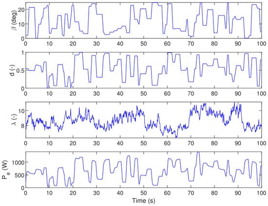
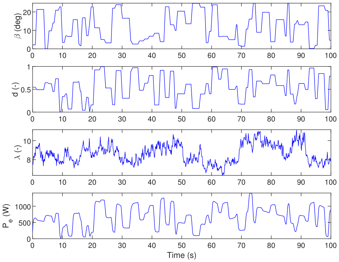
The first step is to construct the full Hankel matrices defined in (84) using the identification data. For this purpose, the turbine is excited using bounded piecewise-constant pseudo-random input sequences, which are subsequently smoothed using a moving-average window of length 5. The blade pitch angle and load-switching duty cycle used for exciting the turbine are shown in Figure 1. In this figure, all data sequences have a length of 1000 samples ($N+L-1=1000$) and the input amplitudes and holding times are selected randomly within their admissible ranges. The sampling period is considered equal to 0.1 s in all simulations of this paper.

Figure 1. System excitation using piecewise-constant pseudo-random input sequences and the corresponding responses.

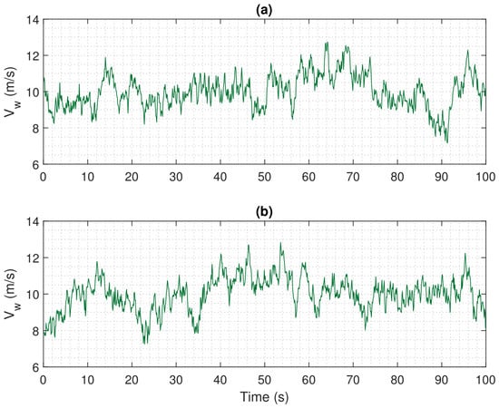
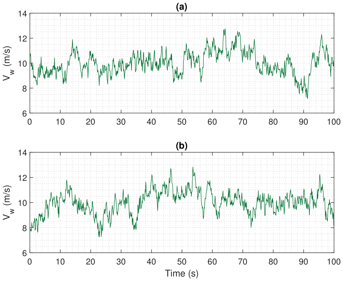
The wind-speed profile used for generating the input–output data and constructing the Hankel matrices is shown in Figure 2a, whereas the wind-speed profile employed in the closed-loop simulations is presented in Figure 2b. To ensure a fair comparison among the different Hankel-matrix reduction methods, exactly the same wind-speed profile shown in Figure 2b was used in all closed-loop simulations, including those based on both the full Hankel matrix and the reduced Hankel matrices. Consequently, any observed differences in the closed-loop responses can be attributed solely to the Hankel-matrix reduction rather than to differences in the wind disturbance.

Figure 2. Wind-speed profiles used in the simulations. (a) Wind-speed realization used for generating the input–output data and constructing the Hankel matrices. (b) Independent wind-speed realization used for evaluating the proposed controller in closed-loop simulations.

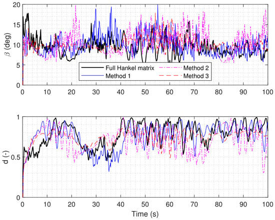
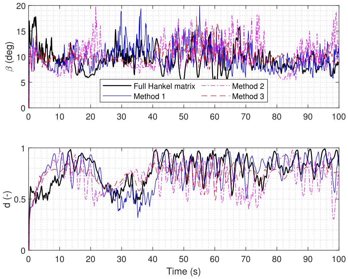
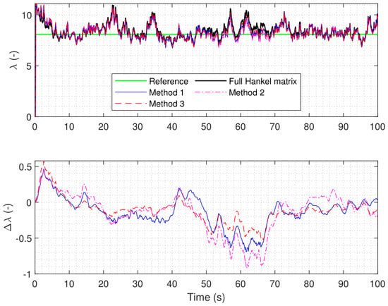
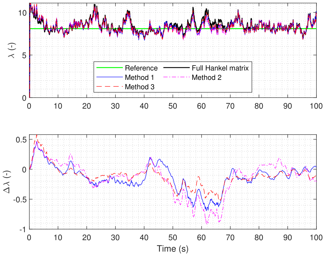
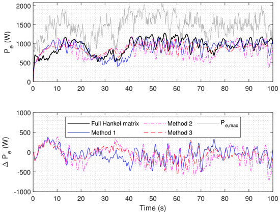
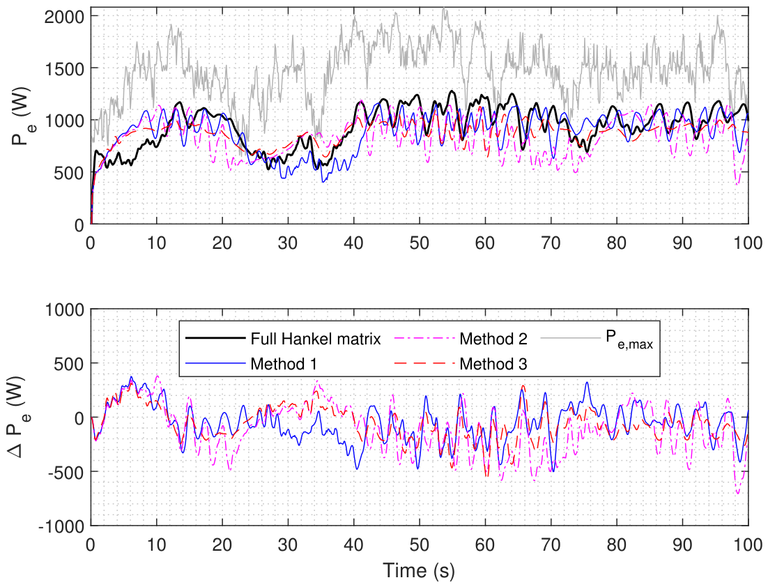
The closed-loop simulation results, in which the control signals are obtained by solving the optimization problem in (94) using the original and reduced-size Hankel matrices, are shown in Figure 3, Figure 4 and Figure 5. In the baseline simulations, the past window and prediction horizon are set to $L_p=L_f=20$. These values were selected through a simple trial-and-error procedure. The sensitivity of the closed-loop results to the choice of $L_p$ and $L_f$ is examined quantitatively later in this section. The selected values for the weights in (93) are $q_i=20$, $q_{\lambda }=200$, $q_p=20$, $q_u=0.1$, and $q_s=1$. There are no universally optimal choices for these weights. They should be selected based on the desired trade-off between control performance and control effort. Figure 3 shows the control signals generated by the controllers, while Figure 4 and Figure 5 present the outputs of the closed-loop control system. In addition to the values of $\lambda$, Figure 4 also depicts the difference between the $\lambda$ obtained using the full Hankel matrix and those obtained using the reduced-size Hankel matrices. Similarly, Figure 5 presents not only the output power but also the difference between the output power obtained using each reduced Hankel matrix and that obtained using the full Hankel matrix, with $\Delta P_e=P_e^{\mathrm{reduced}}-P_e^{\mathrm{full}}$.

Figure 3. Closed-loop control inputs, including the blade pitch angle $\beta$ and the load-switching duty cycle d, obtained using the full Hankel matrix and the three Hankel-matrix reduction methods.

Figure 4. Comparison of the closed-loop tip-speed ratio achieved using the full Hankel matrix and the reduced Hankel matrices obtained by the three column-reduction methods. The lower subplot depicts the deviation of each reduced-order response from the response obtained using the full Hankel matrix.

Figure 5. Comparison of the closed-loop electrical power obtained using the full Hankel matrix and the reduced Hankel matrices generated by the three column-reduction methods. The gray curve represents the approximate maximum extractable electrical power, while the lower subplot depicts the deviation of each reduced-order response from the response obtained using the full Hankel matrix.

The maximum extractable electrical power in Figure 5, denoted as $P_{e,\max }$, is obtained by solving a steady-state optimization problem for each wind-speed sample. For the given wind speed, the blade pitch angle and the duty cycle are swept over their admissible ranges, the corresponding steady-state operating points are computed using the nonlinear turbine model, and the maximum achievable electrical power is recorded as $P_{e,\max }$. Repeating this procedure for all wind-speed samples yields the time-varying maximum-power profile shown in the simulation results.

It should be noted that $P_{e,\max }$ is an approximate quasi-steady benchmark rather than a strict instantaneous upper bound. During transient operation, the generator may temporarily extract part of the kinetic energy stored in the rotating turbine, causing the instantaneous electrical power to exceed the corresponding steady-state value. Such short-term exceedances in Figure 5 therefore do not imply that the steady-state aerodynamic power limit has been violated.

With $N+L-1=1000$ and $L=L_p+L_f=40$, all of the original Hankel matrices defined in (84) have dimensions $40\times 961$. For a fair comparison, the parameters of the three reduction methods were selected such that the resulting reduced Hankel matrices had approximately the same number of columns. In the first method, the maximum admissible relative prediction-map error was set to $\epsilon =0.8\%$. In the second method, the relative prediction-map error threshold was chosen as $\epsilon =5.6\%$. For the third method, the similarity thresholds were selected as ${\epsilon }_G={\epsilon }_O=0.1$, while the maximum admissible relative prediction-map error was set to ${\epsilon }_{\mathrm{map}}=3.2\%$. With these parameter values, the numbers of remaining columns after applying the first, second, and third methods are 483, 484, and 481, respectively, resulting in reduced Hankel matrices of approximately equal size.

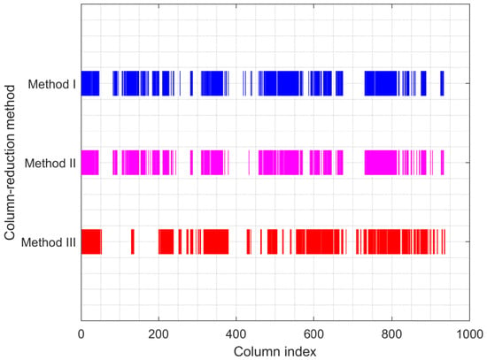
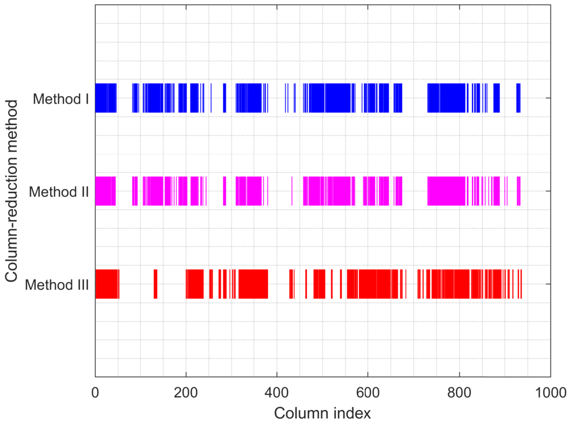
Figure 6 illustrates the indices of the trajectory columns removed by the three proposed reduction methods. Each colored vertical line represents a column eliminated from the original Hankel matrices, while blank locations correspond to the retained columns. The figure provides a visual comparison of the column-selection patterns produced by the three reduction strategies.

Figure 6. Indices of the Hankel-matrix columns eliminated by the three column-reduction methods. Each colored marker corresponds to a removed column. Vertically aligned markers indicate columns eliminated by multiple methods.

To provide a controlled comparison of the three reduction methods, an additional set of simulations was performed at a common prediction-map error level of approximately $\epsilon =1\%$. This comparison was designed to eliminate the effect of using different admissible prediction errors for the three reduction approaches and to provide a more consistent assessment of their computational characteristics.

The full Hankel formulation and the three reduced formulations were compared in terms of the number of retained trajectory columns, reduction ratio, prediction-map error, memory requirement, offline reduction time, and average online QP solution time. The results are summarized in Table 1.

As shown in Table 1, Method 1 provides the largest reduction, retaining 458 of the original 961 columns (52.3% reduction), and decreases the average QP solution time from 490.3 ms for the full formulation to 80.2 ms. Its offline reduction time, however, is 921.7 s. Method 2 requires only 4.35 s for offline reduction, but retains 801 columns (16.6% reduction) and results in an average QP solution time of 317.1 ms. Method 3 retains 633 columns (34.1% reduction), with an offline reduction time of 12.0 s and an average QP solution time of 151.9 ms. The corresponding memory requirements are also reported in Table 1.

To directly assess whether preservation of the prediction map also preserves the actual predictive capability of the reduced models, an additional validation study was performed using input–output data that were not used to construct the Hankel matrices. Three independent validation trajectories were generated from the nonlinear wind-turbine model using different random realizations of the excitation inputs and wind disturbance. For each trajectory, the past output measurements and the future input sequence were used to predict the tip-speed ratio and electrical power over the prediction horizon $L_f=20$. The predictions obtained using the full and reduced Hankel formulations were then compared with the corresponding outputs of the nonlinear wind-turbine model. To provide a controlled comparison among the three reduction methods, the reduced models obtained at the common prediction-map error level of approximately 1%, as reported in Table 1, were used. Table 2 reports the prediction RMSE averaged over the three independent validation trajectories, with the corresponding standard deviations.

Table 2. Multi-step prediction accuracy on independent nonlinear validation trajectories. Values are reported as mean ± standard deviation over three independent realizations.

Method	Reduction (%)	Map Error (%)	${\mathbf{RMSE}}_{\mathit{\lambda }}$	${\mathbf{RMSE}}_{{\mathit{P}}_{\mathit{e}}}$ (W)
Full	0.0	0	$0.757\pm 0.010$	$29.34\pm 1.52$
Method 1	52.3	1.016	$0.782\pm 0.013$	$29.81\pm 1.33$
Method 2	16.6	0.961	$0.757\pm 0.013$	$29.39\pm 1.56$
Method 3	34.1	0.995	$0.777\pm 0.011$	$29.68\pm 1.32$

The results show that the reduced formulations preserve the multi-step prediction accuracy of the full Hankel predictor closely on data generated independently from the nonlinear plant. Method 1 removes 52.3% of the original trajectory columns, while increasing ${\mathrm{RMSE}}_{\lambda }$ from 0.757 to only 0.782 and ${\mathrm{RMSE}}_{P_e}$ from 29.34 W to 29.81 W. Method 2 produces prediction errors that are nearly identical to those of the full formulation, although it provides the smallest reduction in the number of columns. Method 3 again exhibits an intermediate behavior, reducing the number of columns by 34.1% while yielding ${\mathrm{RMSE}}_{\lambda }=0.777$ and ${\mathrm{RMSE}}_{P_e}=29.68$ W. The relatively small standard deviations obtained over the three independent realizations indicate limited variability among the considered validation trajectories. These results provide direct empirical evidence that maintaining a small prediction-map error also preserves the actual multi-step prediction accuracy well for the nonlinear wind-turbine benchmark considered here.

In addition to the computational comparison, the closed-loop performance of the full and reduced formulations was evaluated using the tip-speed-ratio tracking RMSE and the mean generated electrical power. These results are reported in Table 3.

Table 3. Closed-loop performance of the full and reduced Hankel formulations.

Method	${\mathbf{RMSE}}_{\mathit{\lambda }}$	Mean Power (W)
Full	0.884	1019.6
Method 1	0.777	901.8
Method 2	0.886	980.5
Method 3	0.774	851.1

The reduced formulations maintain a tip-speed-ratio tracking accuracy comparable to that of the full formulation. The tracking RMSE is 0.884 for the full formulation and 0.777, 0.886, and 0.774 for Methods 1–3, respectively. The corresponding mean generated powers are 1019.6 W, 901.8 W, 980.5 W, and 851.1 W. Thus, the reduction in the size of the Hankel representation does not result in a systematic deterioration of the tip-speed-ratio tracking performance, although some variation in the generated power is observed among the different formulations.

To examine the sensitivity of the closed-loop results to the selection of the past and prediction horizons, additional simulations were performed for $L_p=L_f=15$, 20, and 25. The full Hankel formulation and Method 3 were considered in this analysis. Method 3 was selected as a representative reduced formulation because, as shown in Table 1, it provides an intermediate trade-off between offline reduction cost and online computational efficiency. All other controller and reduction parameters were kept at their nominal values so that the influence of the horizon lengths could be examined independently. The same wind-speed realization was also used in all cases. The results are summarized in Table 4.

Table 4. Sensitivity of the closed-loop performance to the past and prediction horizons.

	Full Hankel Matrix			Method 3
${\mathit{L}}_{\mathit{p}}={\mathit{L}}_{\mathit{f}}$	${\mathbf{RMSE}}_{\mathit{\lambda }}$	Mean Power (W)	QP (ms)	${\mathbf{RMSE}}_{\mathit{\lambda }}$	Mean Power (W)	QP (ms)
15	0.694	818.5	375.9	0.880	539.5	69.8
20	0.884	1018.8	495.2	0.767	871.8	86.1
25	1.127	1006.1	767.9	0.720	672.3	109.4

The results show that the computational advantage of the reduced formulation is maintained over the investigated range of horizon lengths. For $L_p=L_f=15$, 20, and 25, the average QP solution times of Method 3 are 69.8, 86.1, and 109.4 ms, respectively, compared with 375.9, 495.2, and 767.9 ms for the corresponding full formulations. The tip-speed-ratio tracking performance of Method 3 also remains relatively consistent, with ${\mathrm{RMSE}}_{\lambda }$ ranging from 0.720 to 0.880 over the three cases. In contrast, the mean generated power exhibits greater variation with the horizon length. These results indicate that the substantial reduction in online computational time provided by Method 3 is not limited to the nominal choice $L_p=L_f=20$, although individual closed-loop performance measures can exhibit different sensitivities to the horizon selection.

4.3. Materials and Methods

All simulations reported in this study were performed on a computer equipped with a 13th-generation Intel Core i7-1355U processor (1.70 GHz) and 16 GB of RAM using MATLAB R2023a. The MPC optimization problem in (94) was solved using the quadprog function.

A one-point turbulent wind field was generated using the widely adopted Kaimal turbulence spectrum [29]. The Kaimal model is recommended by the IEC 61400 standard and has been extensively used in wind turbine simulations due to its ability to reproduce realistic atmospheric turbulence characteristics [30]. In the simulations, a prescribed mean wind speed was combined with stochastic turbulent fluctuations synthesized in the frequency domain using randomly generated phases. The resulting wind speed sequence was then used as an external disturbance acting on the wind turbine throughout the simulations. The turbulence intensity was set to $10\%$, while the turbulence length scale was chosen as $L_{\mathrm{turb}}=50\mathrm{m}$. Fixed random seeds were used to ensure reproducibility: seed 1 was used for generating the identification wind realization, seed 2 for the baseline closed-loop simulation, and seeds 2, 3, and 4 for the three independent prediction-validation trajectories.

5. Discussion

The simulation results demonstrate that the stored trajectory set can be substantially reduced without necessarily degrading the closed-loop tracking performance. This observation is supported quantitatively by the additional comparison performed at a common prediction-map error level of approximately $1\%$. The tip-speed-ratio tracking RMSE obtained using the full Hankel formulation is 0.884, compared with 0.777, 0.886, and 0.774 for Methods 1–3, respectively. Thus, despite the reduction in the number of retained trajectories, the tracking accuracy remains comparable to that obtained using the full Hankel matrices. The mean generated power exhibits greater variation, with values of 1019.6 W for the full formulation and 901.8 W, 980.5 W, and 851.1 W for Methods 1–3, respectively. These results indicate that preserving the prediction map within a small tolerance can maintain the essential closed-loop tracking behavior, although it does not guarantee identical closed-loop performance for all performance measures.

The horizon-sensitivity study provides additional evidence that the computational benefit of the reduced formulation is not specific to the nominal choice $L_p=L_f=20$. Over the investigated values $L_p=L_f=15$, 20, and 25, Method 3 consistently requires substantially less online QP solution time than the corresponding full Hankel formulation, while its tip-speed-ratio tracking RMSE remains within a relatively narrow range. The increase in QP solution time with the horizon length is also considerably more pronounced for the full formulation than for the reduced formulation. The generated power, however, is more sensitive to the horizon selection. This observation reinforces the distinction between preservation of the prediction map and invariance of every closed-loop performance measure.

The independent prediction-validation results further support this interpretation. Although the relative prediction-map error is defined using an induced matrix norm and therefore represents a worst-case operator-level measure, the direct prediction tests show that the reduced formulations also retain prediction accuracy under independently generated operating trajectories. At the common prediction-map error level of approximately 1%, the differences between the full and reduced predictors remain small for both the tip-speed ratio and generated electrical power over the 20-step prediction horizon. This empirical result is particularly relevant because the validation trajectories are generated by the nonlinear wind-turbine model, for which the exact LTI trajectory representation underlying the theoretical development is not assumed to hold globally.

The results also support the central idea of this paper, namely that trajectory reduction should be formulated as a prediction-preservation problem rather than a matrix-preservation problem. Existing Hankel reduction techniques generally seek to preserve surrogate properties of the data matrices, such as low-rank structure, approximation error, or numerical conditioning. In contrast, the proposed framework directly evaluates the effect of trajectory removal on the prediction map implemented by the data-driven predictor. Consequently, the retained trajectories are selected according to their contribution to future predictions rather than their contribution to the matrix representation itself.

The computational results reveal distinct trade-offs among the three reduction strategies. At the common prediction-map error level of approximately $1\%$, Method 1 achieves the largest reduction, eliminating 52.3% of the original columns and reducing the average online QP solution time from 490.3 ms for the full formulation to 80.2 ms. This improvement is obtained at the expense of a relatively large offline reduction time of 921.7 s. Method 2 exhibits the opposite behavior: its offline reduction requires only 4.35 s, but it eliminates only 16.6% of the columns and results in an average QP solution time of 317.1 ms. Method 3 provides an intermediate compromise, reducing the number of columns by 34.1% with an offline reduction time of 12.0 s and an average QP solution time of 151.9 ms. The corresponding reductions in Hankel memory requirements follow the same general trend.

These differences are consistent with the computational structures of the three algorithms. Method 1 repeatedly evaluates the prediction-map error during the column-elimination process and therefore achieves the greatest reduction at a high offline computational cost. Method 2 reduces this offline cost by evaluating trajectory importance only once and maintaining a fixed ranking during the reduction process. Method 3 uses inexpensive similarity measures to screen candidate columns before evaluating their effect on the prediction map, resulting in an intermediate balance between offline computational effort and online efficiency. Consequently, no single reduction strategy is uniformly preferable: the appropriate method depends on the relative importance of offline reduction cost, memory usage, and online optimization time in the intended application.

An important advantage of the proposed framework is that it operates directly on the original measured trajectories instead of replacing them with latent basis vectors or low-dimensional projections. Consequently, the reduced predictor retains the Hankel-based representation using original measured trajectory columns and remains fully compatible with existing Hankel-based predictive control formulations. Moreover, the proposed trajectory-selection framework is not restricted to the output-based prediction framework adopted in this paper. The same principle can also be applied to other data-driven predictive control formulations, including conventional DeePC, provided that the corresponding prediction map can be explicitly identified.

Figure 6 further shows that the three reduction algorithms do not necessarily retain the same trajectory columns. Together with the small prediction-map errors reported in Table 1, this indicates that different reduced trajectory sets can approximately preserve the full prediction map, suggesting that the quality of the reduced predictor depends primarily on preserving the underlying input–output mapping rather than on retaining any particular trajectories.

The present work nevertheless has several limitations. The reduction algorithms are currently performed offline after the complete trajectory set has been collected. Furthermore, the proposed framework has been evaluated only through numerical simulations using a nonlinear wind-turbine benchmark, while the theoretical development is established for LTI systems. Experimental validation on physical systems and systematic comparisons with additional state-of-the-art Hankel reduction techniques would further strengthen the conclusions. In addition, explicit closed-loop stability guarantees for the predictive controller under reduced trajectory sets are not established in the present work and remain an open theoretical problem.

Future research will focus on extending the proposed framework to adaptive data-driven predictive control in which the stored trajectory set is updated online as new measurements become available. Another promising direction is the development of more efficient optimization algorithms for prediction-oriented trajectory selection together with theoretical performance guarantees relating prediction-map preservation to closed-loop control performance.

References

- Li, N.; Chen, H.; Li, M.; Yu, S.; Huang, Y. Model predictive control: Past, present, and future. Control Theory Technol. 2026, 24, 173–193. [Google Scholar] [CrossRef] [Scilit]
- Verheijen, P.C.N.; Breschi, V.; Lazar, M. Handbook of linear data-driven predictive control: Theory, implementation and design. Annu. Rev. Control 2023, 56, 100914. [Google Scholar] [CrossRef] [Scilit]
- Li, X.; Yan, M.; Zhang, X.; Han, M.; Law, A.W.K.; Yin, X. Efficient data-driven predictive control of nonlinear systems: A review and perspectives. Digit. Chem. Eng. 2025, 14, 100219. [Google Scholar] [CrossRef] [Scilit]
- Berberich, J.; Allgöwer, F. An overview of systems-theoretic guarantees in data-driven model predictive control. Annu. Rev. Control Robot. Auton. Syst. 2025, 8, 77–100. [Google Scholar] [CrossRef] [Scilit]
- Zhu, J.; Wei, Q.; Yu, X.; Hou, Z. A data-driven predictive control scheme for nonlinear discrete-time systems. IEEE Trans. Cybern. 2025, 55, 3108–3118. [Google Scholar] [CrossRef] [Scilit] [PubMed]
- Coulson, J.; Lygeros, J.; Dörfler, F. Data-enabled predictive control: In the shallows of the DeePC. In Proceedings of the 18th European Control Conference (ECC); IEEE: Piscataway, NJ, USA, 2019; pp. 307–312. [Google Scholar]
- Coulson, J.; Lygeros, J.; Dörfler, F. Regularized and distributionally robust data-enabled predictive control. In Proceedings of the 58th IEEE Conference on Decision and Control (CDC); IEEE: Piscataway, NJ, USA, 2019; pp. 2696–2701. [Google Scholar]
- Berberich, J.; Köhler, J.; Müller, M.A.; Allgöwer, F. Data-driven model predictive control with stability and robustness guarantees. IEEE Trans. Autom. Control 2020, 66, 1702–1717. [Google Scholar] [CrossRef] [Scilit]
- Willems, J.C.; Rapisarda, P.; Markovsky, I.; De Moor, B.L. A note on persistency of excitation. Syst. Control Lett. 2005, 54, 325–329. [Google Scholar] [CrossRef] [Scilit]
- O’Dwyer, E.; Kerrigan, E.C.; Falugi, P.; Zagorowska, M.; Shah, N. Data-driven predictive control with improved performance using segmented trajectories. IEEE Trans. Control Syst. Technol. 2022, 31, 1355–1365. [Google Scholar] [CrossRef] [Scilit]
- Breschi, V.; Chiuso, A.; Fabris, M.; Formentin, S. On the impact of regularization in data-driven predictive control. In Proceedings of the 62nd IEEE Conference on Decision and Control (CDC); IEEE: Piscataway, NJ, USA, 2023; pp. 3061–3066. [Google Scholar]
- Mattsson, P.; Schön, T.B. On the regularization in DeePC. IFAC-PapersOnLine 2023, 56, 625–631. [Google Scholar] [CrossRef] [Scilit]
- Merrikh-Bayat, F.; Mokhtari, M. A linear data-driven model for accurate prediction of the response of non-linear dynamical systems: Application to data-driven output-feedback model predictive controller design. IET Control Theory Appl. 2025, 19, e70095. [Google Scholar] [CrossRef] [Scilit]
- Merrikh-Bayat, F. Output-feedback data-driven model predictive control of nonlinear dynamical systems using a nonlocal model. Syst. Sci. Control Eng. 2025, 13, 2479526. [Google Scholar] [CrossRef] [Scilit]
- Han, S.; Yan, Y.; Bao, J.; Huang, B. A big data-driven predictive control approach for nonlinear processes using behaviour clusters. J. Process Control 2024, 140, 103252. [Google Scholar] [CrossRef] [Scilit]
- Yang, H.; Li, S. A data-driven predictive controller design based on reduced Hankel matrix. In Proceedings of the 10th Asian Control Conference (ASCC); IEEE: Piscataway, NJ, USA, 2015; pp. 1–7. [Google Scholar]
- Zhang, K.; Zheng, Y.; Shang, C.; Li, Z. Dimension reduction for efficient data-enabled predictive control. IEEE Control Syst. Lett. 2023, 7, 3277–3282. [Google Scholar] [CrossRef] [Scilit]
- Kramer, B.; Gorodetsky, A.A. System identification via CUR-factored Hankel approximation. SIAM J. Sci. Comput. 2018, 40, A848–A866. [Google Scholar] [CrossRef] [Scilit]
- Vahidi-Moghaddam, A.; Zhang, K.; Yin, X.; Srivastava, V.; Li, Z. Online reduced-order data-enabled predictive control. IEEE Trans. Autom. Sci. Eng. 2025, 22, 22455–22467. [Google Scholar] [CrossRef] [Scilit]
- Shi, J.; Lian, Y.; Jones, C.N. Efficient recursive data-enabled predictive control. In Proceedings of the 2024 European Control Conference (ECC); IEEE: Piscataway, NJ, USA, 2024; pp. 880–887. [Google Scholar]
- Faye-Bedrin, A.; Aranovskiy, S.; Chauchat, P.; Bourdais, R. A computationally efficient reformulation for data-enabled predictive control. In Proceedings of the 2024 IEEE 63rd Conference on Decision and Control (CDC); IEEE: Piscataway, NJ, USA, 2024; pp. 4855–4860. [Google Scholar]
- Lazar, M.; Verheijen, P.C.N. Generalized data-driven predictive control: Merging subspace and Hankel predictors. Mathematics 2023, 11, 2216. [Google Scholar] [CrossRef] [Scilit]
- Zhang, X.; Zhang, K.; Li, Z.; Yin, X. Deep DeePC: Data-enabled predictive control with low or no online optimization using deep learning. AIChE J. 2025, 71, e18644. [Google Scholar] [CrossRef] [Scilit]
- Schmitz, P.; Schaller, M.; Voigt, M.; Worthmann, K. Fast and memory-efficient optimization for large-scale data-driven predictive control. IFAC-PapersOnLine 2024, 58, 220–225. [Google Scholar] [CrossRef] [Scilit]
- Lawrence, N.; Loewen, P.; Wang, S.; Forbes, M.; Gopaluni, B. Deep Hankel matrices with random elements. In Proceedings of the 6th Annual Learning for Dynamics & Control Conference (L4DC); PMLR: Birmingham, UK, 2024; pp. 1579–1591. [Google Scholar]
- Golub, G.H.; Van Loan, C.F. Matrix Computations, 4th ed.; JHU Press: Baltimore, MD, USA, 2013; Volume 3. [Google Scholar]
- Burton, T.; Jenkins, N.; Sharpe, D.; Bossanyi, E. Wind Energy Handbook, 2nd ed.; John Wiley & Sons: Hoboken, NJ, USA, 2011. [Google Scholar]
- Heier, S. Grid Integration of Wind Energy Conversion Systems, 2nd ed.; John Wiley & Sons: Hoboken, NJ, USA, 2006. [Google Scholar]
- Kaimal, J.C.; Wyngaard, J.C.; Izumi, Y.; Coté, O.R. Spectral characteristics of surface-layer turbulence. Q. J. R. Meteorol. Soc. 1972, 98, 563–589. [Google Scholar] [CrossRef]
- IEC 61400-1; Wind Energy Generation Systems—Part 1: Design Requirements, 4th ed. International Electrotechnical Commission: Geneva, Switzerland, 2019.
Disclaimer/Publisher’s Note: The statements, opinions and data contained in all publications are solely those of the individual author(s) and contributor(s) and not of MDPI and/or the editor(s). MDPI and/or the editor(s) disclaim responsibility for any injury to people or property resulting from any ideas, methods, instructions or products referred to in the content. |
© 2026 by the author. Licensee MDPI, Basel, Switzerland. This article is an open access article distributed under the terms and conditions of the Creative Commons Attribution (CC BY) license.