


Abstract
Vibrations generated during cutting in machining processes present a significant challenge, directly impacting surface quality, tool longevity, and processing efficiency. Accurate modeling of vibration behavior under varying cutting conditions is therefore essential for advancing the understanding of machining dynamics. In this research, triaxial vibration accelerations in the tool holder region during CNC milling of Al 6061 material were experimentally measured. The proposed framework focuses on the prediction of process-level time-domain acceleration responses rather than high-frequency chatter or tooth-passing vibration components. The experiments incorporated a range of spindle speeds, feed rates, and depths of cut. The resulting multi-axial acceleration time series were modeled using deep learning-based time series approaches to capture complex and nonlinear dynamics. Specifically, Long Short-Term Memory (LSTM) and Gated Recurrent Unit (GRU) architectures were developed, and their generalization capabilities were assessed using the Leave-One-Experiment-Out (LOEO) method. Comparative analyses employing root mean square error (RMSE), mean absolute error (MAE), and coefficient of determination (R2) metrics indicate that both models reliably predict multi-axis acceleration responses. Notably, the LSTM architecture demonstrates a more balanced learning performance for representing long-term dynamics. These findings provide an effective, practical approach to data-driven modeling of vibrations in CNC milling processes.
1. Introduction
Dynamic vibrations generated during CNC milling operations significantly influence surface quality, tool life, and process stability. Under high-speed, variable cutting conditions, accurately modeling the time-dependent vibration behavior in the tool holder region is essential to ensuring the reliability of the production process. Traditional analytical and experimental methods are limited in their ability to capture these complex, nonlinear dynamics. The increasing volume of data and the complexity of processing underscore the need for data-driven modeling approaches. Time-series-based deep learning models provide a robust alternative for predicting vibration behavior in CNC machining processes.
The literature presents various methods for investigating vibrations in CNC machining. Early studies examined the relationships between cutting parameters and vibration amplitudes using experimental and statistical techniques. More recently, machine learning and deep learning-based approaches have attracted considerable attention for vibration prediction, owing to their capacity to model complex temporal dependencies. Recurrent neural network architectures, particularly LSTM and GRU models, are now widely adopted for their effectiveness in representing both transient and stable dynamics during machining.
Ford et al. introduce an approach that analyzes the structural vibration behavior of machine tools, aiming to manage these vibrations through adaptive control strategies to enhance machine tool performance [1]. Li et al. examined the effects of structural vibrations on machining quality and efficiency in CNC machine tools, demonstrating that the dynamic characteristics of the machine structure can be more effectively determined using modal analysis based on operational shock excitation [2]. Yesilyurt and Öztürk utilized cutting tool vibration analysis in milling to identify the presence and progression of damage to the milling cutter [3]. Bhogal et al. studied the impact of cutting parameters on tool vibration and surface roughness during end milling of EN-31 tool steel [4]. Shihan et al. analyzed vibrations generated during end milling of hardened Monel (K-400) alloy, evaluating the effects of spindle speed, feed rate, and cutting depth on vibration behavior and tool wear. Their findings indicate that spindle speed is a decisive parameter affecting vibration amplitude, and that analyses based on feed acceleration are effective in predicting vibrations [5]. Wszołek et al. emphasize the importance of real-time monitoring and analysis of vibration data from CNC milling machines within the Industry 4.0 framework for traceability and optimization of production processes [6]. Wang et al. highlight the critical role of vibration in CNC milling quality and demonstrate the necessity of real-time monitoring of vibration behavior using a hardware- and software-based measurement system [7]. Uwajambo and Thakur combined finite element methods with numerical and experimental modal analysis to determine the vibration-induced dynamic behavior of a CNC milling machine, revealing the machine’s resonance frequencies, mode shapes, and structural weaknesses [8]. Chen et al. established that the relationship between tool vibration and surface roughness can be elucidated by processing cutting tool vibration signals in precision milling using singular spectrum analysis, and that feed rate and cutting depth negatively impact surface quality by increasing vibration levels [9]. To effectively model the complex, nonlinear structure of vibration data, artificial intelligence and deep learning-based approaches have been adopted to surpass traditional methods. Mohd Ghazali and Rahiman systematically reviewed 105 studies on vibration-based machine monitoring and diagnosis and highlighted the prominent role of vibration analysis in condition monitoring, noting that vibration-based approaches account for more than 82% of fault-diagnosis techniques reported in the literature; they also emphasized the increasing use of deep learning for automatic feature extraction from raw vibration signals [10]. Raju et al. report that surface roughness can be predicted with high accuracy using machine-learning-based regression models that leverage frequency-domain features of spindle-bearing-induced vibrations in CNC milling operations [11]. Karabacak employed STFT-based spectrograms of vibration, acoustic-emission, and motor-current signals to classify CNC milling tool-wear stages using pretrained CNN architectures; with larger spectrogram sets, ResNet-50-based models achieved validation and test accuracies above 90%, while selected EfficientNet-B0 models reached 100% validation and test accuracy [12]. Kaliyannan et al. compared LSTM, FFNN, Q-learning, and SARSA models for vibration-based tool condition monitoring in milling and reported classification accuracies of 94.85%, 98.16%, 98.50%, and 98.66%, respectively, with SARSA achieving the highest performance [13]. Tambake et al. indicate that machine learning-based fault diagnosis achieves high accuracy using statistical features extracted from three-axis vibration data in CNC milling, offering an effective solution for real-time predictive maintenance [14]. Iqbal et al. find that a deep learning-based approach trained on time–frequency representations of vibration and acoustic signals achieves high classification accuracy for early diagnosis of bearing failures in CNC machines, even in noisy conditions [15]. Oleaga et al. combined experimentally measured frequency-response functions, analytical chatter calculations, and machine-learning models to predict critical cutting depth and chatter frequency in heavy-duty milling; Random Forest achieved the best performance, with RMSE values of approximately 0.95 mm for critical depth and 7.3 Hz for chatter frequency under a 10 × 10 cross-validation scheme [16]. Gao et al. developed a vibration-signal-based surface roughness prediction framework for robotic face milling by combining DFT–SVMD signal processing with a hybrid kernel extreme learning machine, achieving a test MAE of 0.073 μm and RMSE of 0.092 μm and outperforming single-kernel ELM, SVM, and ANN models [17]. Finkeldey et al. find that AI-based data-driven models analyzing vibration data from milling operations enable more accurate prediction of tool vibrations under variable machining conditions [18]. Vinchon et al. demonstrate that real-time, high-accuracy monitoring of cutting tool status is achievable by analyzing features extracted from vibration signals during milling operations using machine-learning-based models [19]. Shah et al. combined Morlet-wavelet scalograms, SinGAN-based data augmentation, and LSTM architectures for tool-wear prediction in face milling, reporting a test MAE of 0.005, RMSE of 0.016, MSE of 0.0002, and R2 of 0.997 for the stacked LSTM model using vibration-derived features [20]. Hu et al. report that LSTM- and GRU-based deep learning models, trained on time-series vibration data and machining parameters, achieve high accuracy in directly predicting vibration and quantifying its intensity in milling operations [21]. Li et al. demonstrate that deep learning-based data-driven models can predict forces at clamping points under variable machining conditions in milling operations with high accuracy by considering temporal relationships [22]. Although the present study focuses on milling, selected studies from other machining processes were also considered where directly comparable sensing hardware, time-domain tri-axial acceleration measurements, and data-driven process-level vibration prediction frameworks were employed, since these methodological elements are transferable across machining operations. Eski modeled experimentally measured time-domain tri-axial acceleration responses of a CNC drilling process using ANN predictors at different spindle speeds, including 1500 rpm, demonstrating the use of such signals for process-level vibration response prediction [23]. Similarly, Esim and Yıldırım used Brüel & Kjær 3560-B IDA and 4524-B-001 tri-axial accelerometer measurements to model time-domain acceleration responses of a drilling process using ANN predictors under 1000 and 1500 rpm spindle speeds [24]. Çetinkaya et al. used time-domain acceleration responses measured from CNC turning experiments with a Brüel & Kjær 4524-B-001 tri-axial accelerometer and 3560-B IDA system for ANN-based process-level vibration response prediction, collecting 601 vibration data points over a 45 s machining interval under different spindle speed and feed rate conditions [25]. Recent studies have further highlighted the growing role of advanced predictive frameworks in improving machining accuracy, process monitoring, and adaptive manufacturing performance. Xu et al. developed a digital-twin-driven TCN-BiLSTM framework for intelligent tracking-error prediction and compensation in ultra-precision machining, demonstrating how deep temporal models can support not only accurate process-state prediction but also direct machining-error compensation. Their optimized model achieved minimum MAE values of 0.000009 and 0.000023 for the X- and Y-axis tracking errors, respectively, while the resulting compensation strategy reduced the corresponding tracking errors by approximately 45–75% and 40–70% [26]. Liu et al. used a 1-DCNN to identify hydraulic-press operating phases from power-consumption time-series data, achieving 98.89% test accuracy and demonstrating the potential of deep learning for automated feature learning and real-time industrial monitoring [27]. Yin et al. established a continuum-mechanics-based microstructure prediction model for ultrasonic vibration machining, achieving 97.3% accuracy in dislocation-density prediction and 92.6% in grain-size prediction, while reducing the need for extensive machining trials and costly material characterization [28]. Yin et al. showed that ultrasonic vibration parameters strongly influence strain-rate-dependent material removal in tungsten alloys, with increasing phase difference improving plastic deformation and reducing surface roughness to 32 nm [29]. He et al. proposed a feature-decoupling and domain-adaptive framework for cross-condition tool wear prediction, achieving R2 values of 0.9112, 0.8583, and 0.8407 across three NASA milling target conditions and demonstrating strong generalization under varying machining conditions [30].
However, the reviewed studies predominantly focus on tool condition, surface roughness, chatter, force, or wear prediction, while the direct prediction of future multi-axis time-domain acceleration responses remains comparatively less explored. The present study addresses this gap by jointly considering machining parameters and preceding acceleration histories within an experiment-level validation framework.
This study uses LSTM and GRU deep learning models to capture the time-dependent patterns present in acceleration data from CNC milling experiments. The purpose of model training is not merely to reproduce measured acceleration signals, but to learn the temporal relationship between cutting parameters, previous acceleration histories, and future process-level acceleration responses. Such predictive capability can support intelligent process monitoring, early identification of abnormal dynamic behavior, and digital-twin-based estimation of machining response. To rigorously assess model generalizability across varying experimental conditions, a Leave-One-Experiment-Out (LOEO) validation strategy was implemented, ensuring the integrity of each experiment. Since each CNC machining experiment features distinct cutting parameters and dynamic behaviors, random data splitting or traditional cross-validation methods may yield overly optimistic performance estimates due to intra-experimental correlations. The LOEO approach, therefore, offers a strong and reliable framework for evaluating the predictive performance of LSTM and GRU models on previously unseen experimental conditions.
Details regarding the experimental setup, data collection, signal preprocessing, model development, and validation strategy are provided in the Materials and Methods section. The Experimental Results section presents performance evaluations and comparative analyses based on results from diverse experimental conditions. The Conclusion and Discussion section interprets the findings with respect to processing, model generalizability, and industrial applicability.
The originality of this study lies in the integrated formulation of experiment-level multi-axis acceleration prediction for CNC milling. Specifically, the study makes three main contributions: (i) a one-step-ahead prediction framework that simultaneously estimates the ax, ay, and az acceleration components using previous multi-axis acceleration histories together with feed rate, spindle speed, and depth of cut; (ii) an experiment-level LOEO validation strategy in which complete machining runs are withheld from model training, enabling a rigorous assessment of generalization to unseen experimental runs while preserving experiment integrity; and (iii) a controlled comparison of LSTM and GRU architectures with MLP, 1D-CNN, and Transformer Encoder benchmarks using the same input variables, prediction targets, windowing procedure, normalization strategy, and LOEO fold assignments. These contributions are evaluated using experimentally acquired CNC milling data obtained under systematically varied machining conditions.
Accordingly, the following research questions were formulated: RQ1: To what extent can LSTM and GRU models predict multi-axis time-domain acceleration responses in CNC milling using machining parameters and previous acceleration histories? RQ2: How effectively can these models generalize to unseen experimental runs under a leave-one-experiment-out validation strategy? RQ3: How do LSTM and GRU models compare in terms of prediction performance across different acceleration axes and machining conditions?
2. Materials and Methods
Accurate monitoring and modeling of vibrations generated during CNC milling operations are essential for maintaining surface quality and extending tool life. Dynamic oscillations, especially in the tool holder area and near the spindle, intensify with changes in cutting forces, which, in turn, influence system rigidity, machining stability, and overall production performance. In this study, triaxial acceleration data were collected experimentally during the milling of Al 6061 material using a triaxial accelerometer positioned in the tool holder area under varying cutting parameters, including feed rate, depth of cut, and rotational speed. The resulting multi-axis time series were subsequently analyzed using deep learning-based LSTM and GRU models to model and predict the multi-axis acceleration responses generated during the cutting process.
2.1. Experimental Setup and Instrumentation
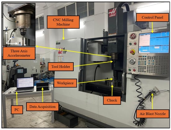
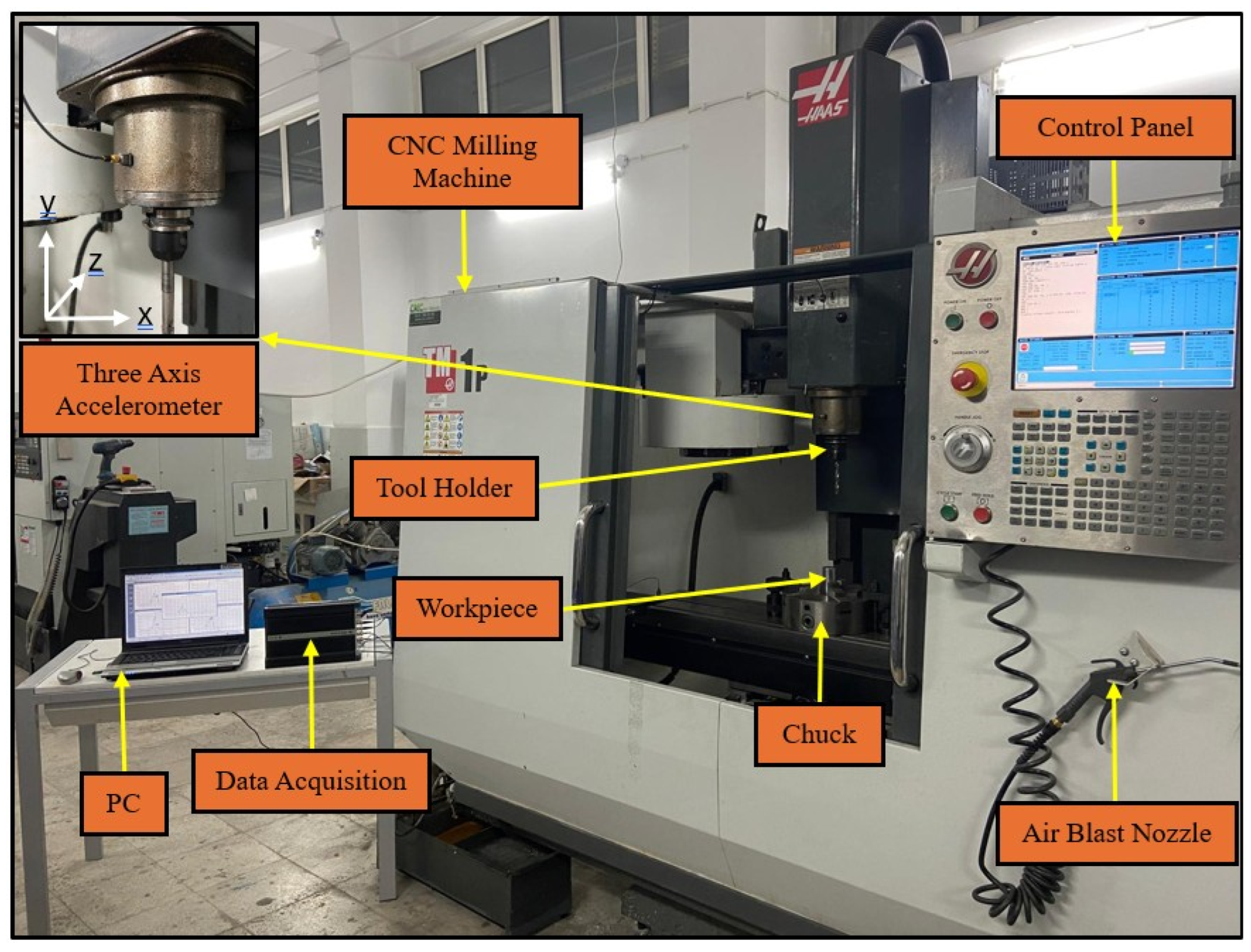
The CNC milling machine employed in this study features precise positioning along the x, y, and z axes and supports multi-axis machining. Real-time vibration monitoring during the milling process was achieved by mounting a Brüel & Kjær 4524-B-001 (Brüel & Kjær, Nærum, Denmark) three-axis accelerometer on the tool holder. According to the manufacturer’s specifications, the sensor has a nominal voltage sensitivity of 1 mV/(m/s2) with a ±10% sensitivity tolerance and a measurement range of ±5000 m/s2 (±500 g), with the specified sensitivity tolerance providing the relevant sensor-level indication of measurement variability. Acceleration signals were transmitted to a computer using the Brüel & Kjær 3560-B (Brüel & Kjær, Nærum, Denmark) Intelligent Data Acquisition (IDA) system, which provides high-accuracy data acquisition. The Al 6061 alloy workpiece was secured to the machine using appropriate clamping elements, and all machining parameters were programmed and executed through the CNC control panel. Figure 1 presents the general schematic layout of the experimental setup.
Figure 1.
Experimental setup.
Table 1 presents the technical specifications of the CNC milling machine utilized in this study.
Table 1.
Features of the CNC Milling Machine used in the Experimental System.
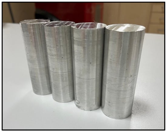
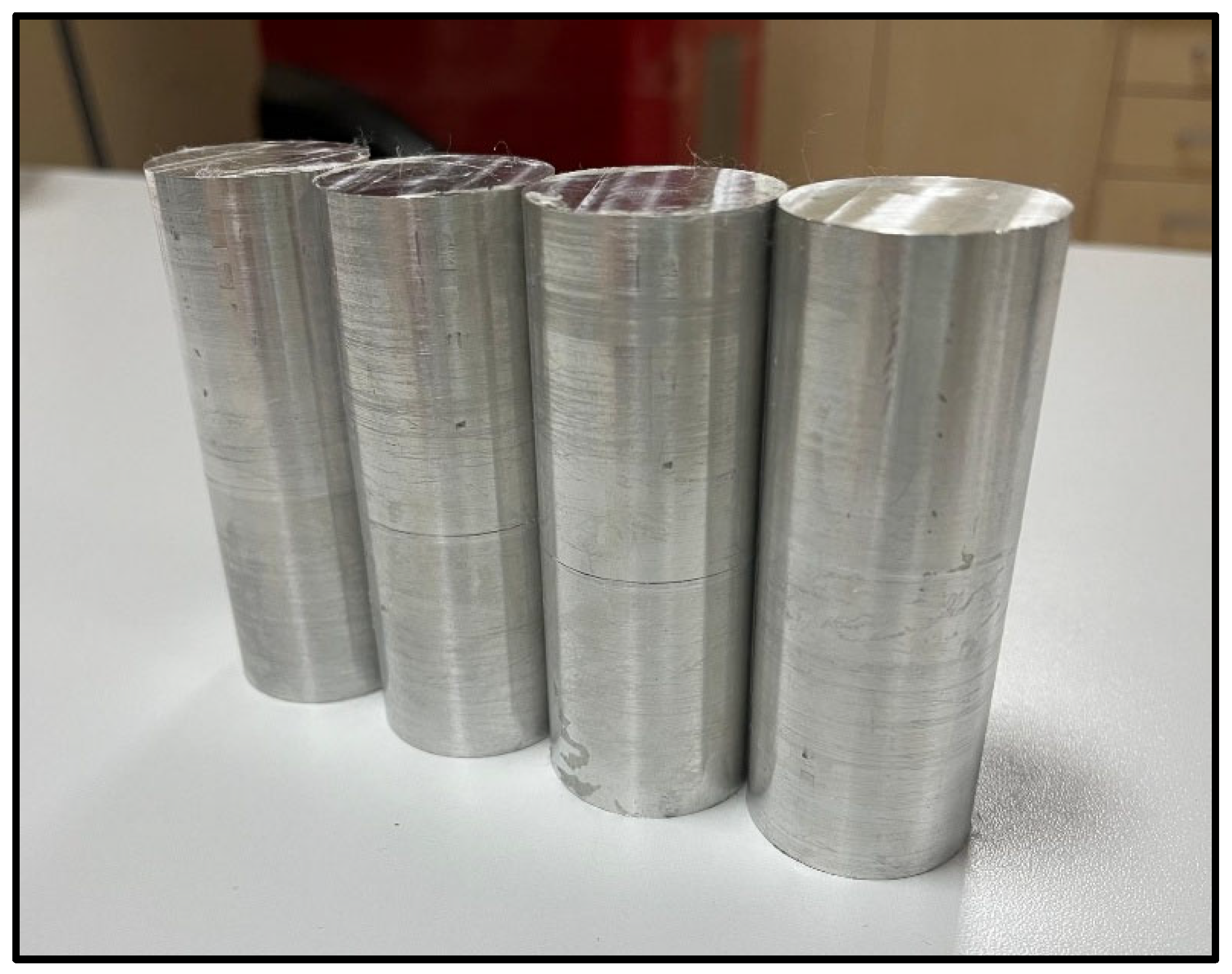
All experiments were conducted under dry-cutting conditions to prevent potential alterations in the material’s physical and mechanical properties caused by coolant. All experimental runs were performed on the same CNC milling machine under the same laboratory environmental conditions to maintain consistency across the experiments. Following each experiment, chips accumulated in the process area were removed using compressed air to ensure clean, repeatable working conditions, thereby facilitating comparability across experiments. Cylindrical Al 6061 workpieces with a diameter of 30 mm and a length of 100 mm, as illustrated in Figure 2, were used in the milling tests.
Figure 2.
Workpiece used in the Experimental System.
To clarify the rationale for material selection, the principal physical and mechanical properties of Al6061 and Al7075 are summarized in Table 2.
Table 2.
Physical and mechanical properties of Al6061 and Al7075 workpiece materials.
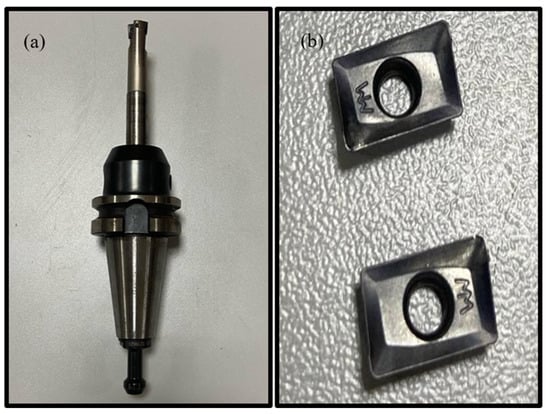
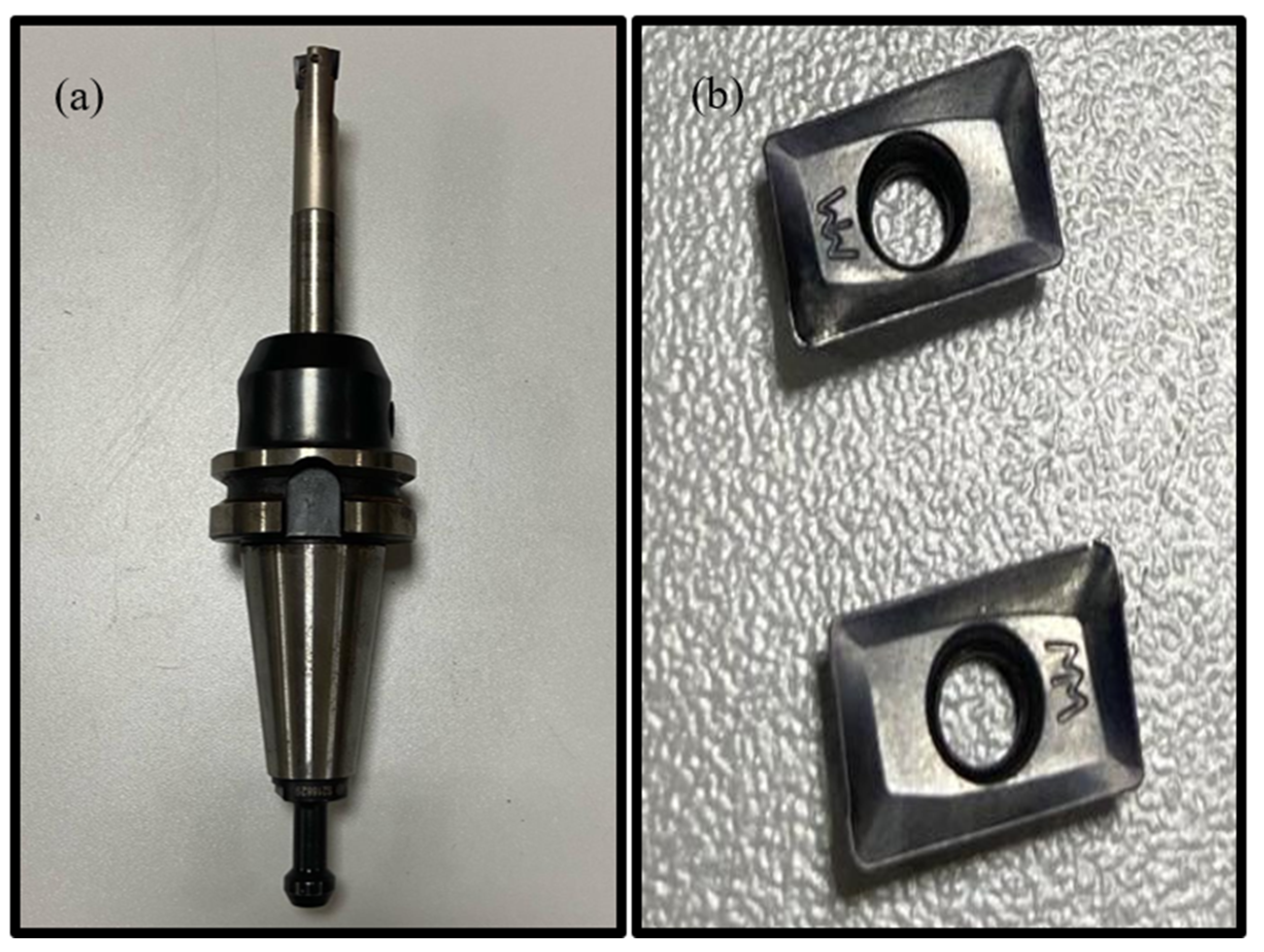
The selection of Al6061 and Al7075 was intended to provide two materially distinct aluminum alloys within the same machining framework. As summarized in Table 2, the two alloys exhibit notable differences in their mechanical and thermal properties. These differences provide a suitable basis for evaluating whether variations in material characteristics are reflected in the measured multi-axis acceleration responses under comparable machining conditions. The milling experiments were performed using a 16 mm diameter indexable end mill equipped with two active APKT 100304 PDTR carbide inserts. The cutter had a shank diameter of 16 mm, an overall length of 100 mm, a cutting-section length of 25 mm, and a maximum axial cutting capacity of 9 mm. Each insert had a nominal corner radius of 0.40 mm. The same cutter, insert configuration, and tool-overhang setting were maintained throughout all experiments to keep tool-related geometric effects constant. A new pair of inserts was installed before each experiment; therefore, cumulative tool wear was not carried over between experimental runs, and no wear-threshold-based replacement criterion was required. Accordingly, feed rate, spindle speed, and axial depth of cut were treated as the varying machining parameters in the prediction models. The tool holder and the milling insert used in the experiments are shown in Figure 3a and Figure 3b, respectively.
Figure 3.
Cutting tool used in the experimental system. (a) Tool Holder. (b) Milling Insert.
2.2. Cutting Parameters
The milling tests in this study were conducted using a two-level, three-factor full-factorial design (23), with feed rate, spindle speed, and depth of cut selected as the primary variables. The factor levels were determined by considering the operating capability of the CNC milling machine and parameter ranges reported in the relevant milling literature, while keeping the experiments within a stable operating range without imposing excessive mechanical loading on the machine-tool system. These predefined levels were then combined systematically to generate the eight experimental conditions presented in Table 3.
Table 3.
Cutting parameters used in the experiment.
For subsequent modeling, the recorded acceleration histories were exported as sequential time-domain data with an approximate temporal spacing of 0.08 s between consecutive records. Therefore, the scope of the present work is not the identification of high-frequency spindle harmonics, tooth-passing frequency components, or chatter-related spectral phenomena. Instead, the study focuses on the prediction of process-level time-domain acceleration response trends observed during CNC milling under different cutting conditions. This sampling structure is suitable for modelling the temporal evolution of macro-scale acceleration variations associated with tool–workpiece engagement, cutting pass transitions, and load-dependent dynamic response over the machining interval. This process-level interpretation is also supported by previous ANN-based machining studies using time-domain acceleration responses. Accordingly, the proposed LSTM and GRU models are evaluated as data-driven predictors of multi-axis acceleration responses rather than as frequency-domain chatter or high-frequency vibration diagnostic models.
Each of the eight experiments was evaluated as an independent scenario in the analyses conducted for this study. This approach facilitates a comparative examination of the effects of parametric changes on vibration behavior.
The feed values were defined as feed per revolution and were set to 0.05 and 0.10 mm/rev; therefore, they do not represent feed per tooth. The radial width of cut (ae) was maintained at approximately 12 mm, while the cutter diameter (D = 16 mm), number of active inserts (Z = 2), cutter geometry, insert configuration, and tool-overhang setting remained constant throughout the experiments.
All cutting parameter combinations used in the study are presented in Table 3, along with their corresponding Experimental IDs.
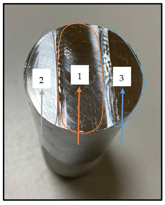
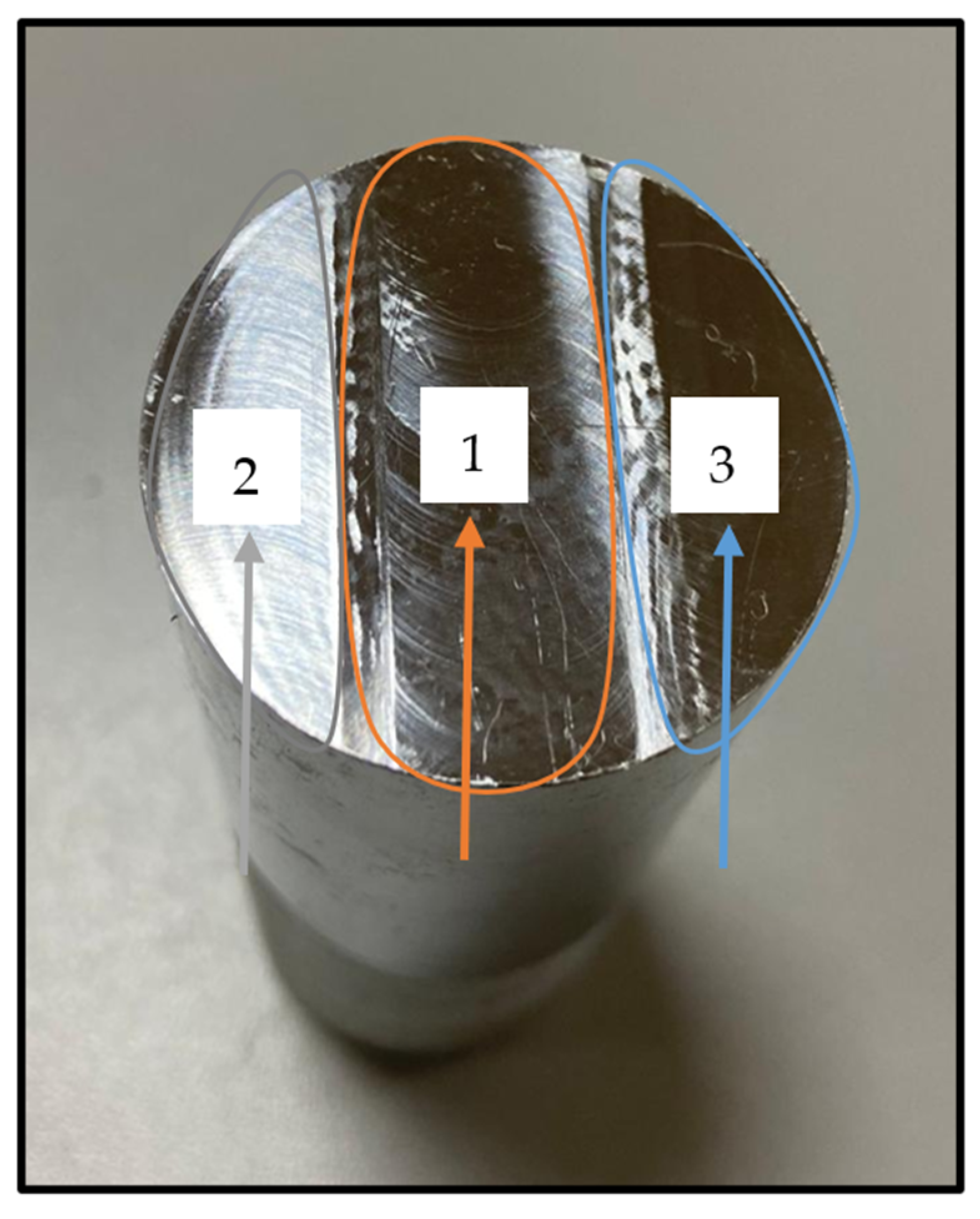
The machined profile consisted of three consecutive passes over the workpiece surface, with the operational sequence illustrated schematically in Figure 4. The three distinct wave periods identified in the vibration signals, as analyzed in Section 3, correspond directly to the successive shear transitions. Regions labeled 1, 2, and 3 in the figure indicate the vibration responses associated with the first, second, and third cutting passes, respectively.
Figure 4.
Cutting order on the Workpiece.
Fundamental cutting parameters, including feed, depth of cut, radial cut width, and cutting speed, are physical quantities that influence the loads generated during tool-workpiece interaction and chip formation. Theoretical representations of these parameters are provided by equations for feed rate, chip cross-sectional area, metal removal rate, and cutting speed, which describe the mechanical effects of the cutting process. The following equations describe the physical conditions used in this study.
, as presented in Equation (1), denotes the feed rate (mm/min) and is calculated by multiplying the spindle speed (rev/min) by the feed amount (mm/rev). This parameter is a primary determinant of the cutting load, as it quantifies the distance the tool travels along the workpiece per unit time. The nominal material removal cross-sectional area was calculated as follows:
where denotes the nominal material removal cross-sectional area (mm2), is the axial depth of cut (0.5 or 1.0 mm), and is the radial width of cut, which was maintained at approximately 12 mm throughout the experiments. The nominal cutter diameter was 16 mm; therefore, represents the actual radial engagement rather than the full cutter diameter.
, as presented in Equation (3), represents the material removal rate (MRR) (mm3/min). It was calculated using the nominal material removal cross-sectional area and the feed speed. This parameter quantifies the nominal volume of material removed per unit time and is used as an indicator of the cutting load imposed by the selected machining conditions.
In Equation (4), denotes the cutting speed (m/min), denotes the tool diameter, and represents the spindle speed. Cutting speed, the peripheral velocity of the tool’s cutting edge, significantly influences material machinability, thermal effects, and tool wear.
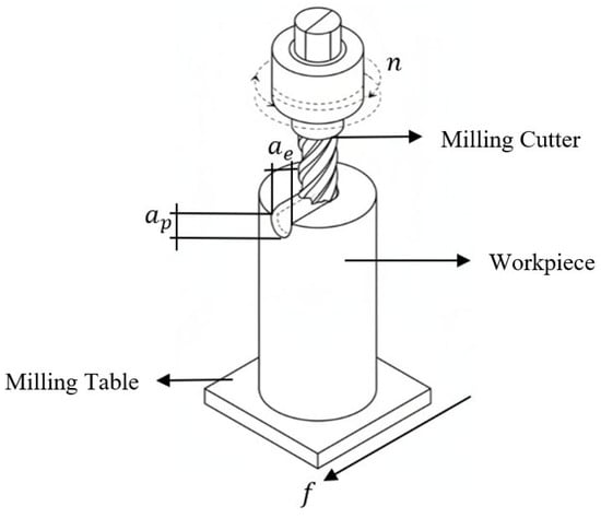
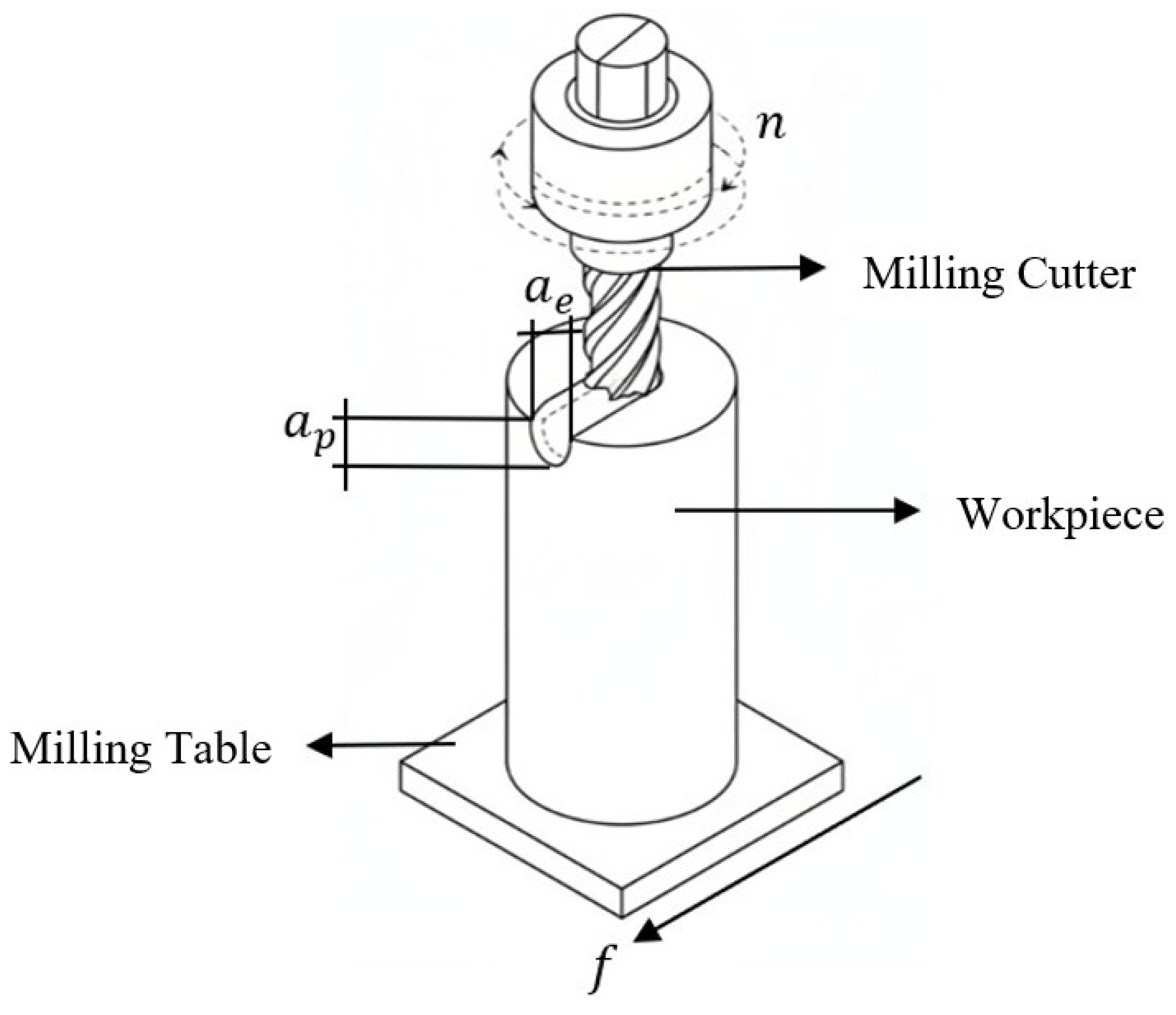
Figure 5 illustrates the geometric equivalents of fundamental cutting parameters in milling operations, presented in both simple and isometric views. The depiction of tool geometry entering the cylindrical workpiece from the exterior visually clarifies the physical relationships among parameters such as cutting speed, feed rate, depth of cut, and chip width, as defined in Equations (1)–(4).
Figure 5.
Geometric equivalents of cutting parameters used in milling operations.
2.3. Data Acquisition
Acceleration signals were acquired from the tool-holder-mounted triaxial accelerometer using the Brüel & Kjær measurement system, which was configured over a frequency range of 0–3.2 kHz. Acceleration was expressed in m/s2. The recording duration varied among the machining conditions and extended up to approximately 196 s. This variation resulted in time series of differing lengths for each experimental scenario. The measured axial acceleration components (ax, aᵧ, az) were essential for characterizing the machine’s dynamic response to cutting forces and its structural vibration properties. Signals recorded along the three axes served as the primary data source for analyzing transient oscillations during the process and the dynamic characteristics of stable cutting regions. Vibrations generated during milling were measured using a three-axis accelerometer affixed to the tool holder region with high-strength industrial adhesive, with sensor axes aligned to the coordinate system depicted in Figure 1. The sensor surface was protected with an insulating layer to prevent chip accumulation and associated micro-vibrations. Accelerometer signals were transmitted to the IDA data acquisition unit via low-noise coaxial cables and recorded at the specified sampling frequency. The cabling was regulated to minimize errors from electromagnetic interference and mechanical contact. Sensor alignment and mounting integrity were verified before each experiment to ensure measurement repeatability.
2.4. Preprocessing
In this study, vibration signals and process parameters were organized by experiment number and time sequence before adaptation for deep learning models. Each input sequence consisted of 48 consecutive records. Considering the approximately 0.08 s spacing of the exported time-history data, each input window represented about 3.84 s of temporal information. Each window included six input variables, and the target output comprised three-axis acceleration values at a future time point. To assess the model’s generalization across experiments, the dataset was partitioned using a LOEO approach: each experiment was sequentially designated as the test set, the next as the validation set, and the remaining experiments as the training set. This approach was selected to evaluate the model’s generalization capacity across varying shear conditions. The scenario based on the LOEO approach is presented in Table 4.
Table 4.
Scenario determined using the LOEO approach.
To clarify the actual size and structure of the dataset, Table 5 summarizes the experimental design, the number of time-domain records obtained from each experiment, the total number of acceleration observations, and the validation strategy used in this study.
Table 5.
Dataset structure used for model training and validation.
All input and output variables were standardized using the StandardScaler method. Conversion coefficients were derived exclusively from the training data and subsequently applied to the validation and test datasets. This approach ensured consistent, normalized, and multivariate time series samples across all experiments.
Model training was conducted in the Google Colab environment using Python 3.13.15 and TensorFlow 2.20.0, with an NVIDIA T4 GPU accelerator. All training procedures were executed on a GPU-powered computing platform.
2.5. Model Architectures
This study employed iterative learning-based deep learning architectures to model the dynamic structure of multivariate vibration time series collected during milling operations. These architectures, which explicitly represent temporal dependencies, enable the prediction of both long-term relationships in stable cutting regions and abrupt amplitude changes in transition regions. Two widely used feedback deep learning approaches, each with distinct gate mechanisms and computational characteristics, were selected for comparative assessment of their capacity to represent and generalize vibration signals. LSTM and GRU architectures were chosen for their effectiveness in modeling vibration signals with dominant temporal dependencies and their established presence in the literature.
To clarify that model convergence was not judged only from the training loss, the convergence control and model selection strategy used during training is summarized in Table 6.
Table 6.
Convergence control and model selection configuration.
2.5.1. LSTM Architecture
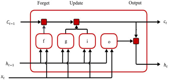
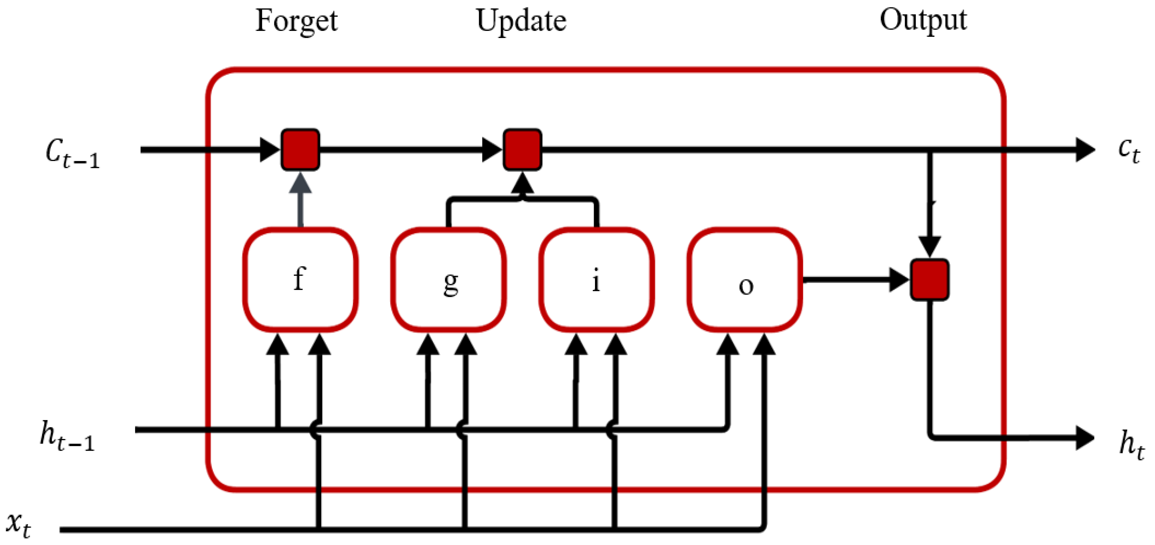
The long short-term memory (LSTM) architecture uses gates to solve the gradient vanishing problem in classical recurrent neural networks. These gates help control the flow of information in the cell state. The forget gate decides what information to keep. The input gate controls what new information is added to the cell state. The output gate sends certain information to the output. Figure 6 shows how these gates update the cell state and hidden state over time.
Figure 6.
Cell structure of the LSTM model.
These gate mechanisms are calculated using sigmoid and hyperbolic tangent activation functions with the input vector and the previous latent state. The cell state is updated by scaling the information from the previous state with a forgetting gate and adding new candidate information via the input gate. Finally, the updated cell state is filtered by the output gate to obtain the latent state vector. Thanks to this mathematical structure, the LSTM model can effectively capture long-term dependencies and stable dynamic behaviors in vibration signals during the milling process.
The internal dynamics of an LSTM cell are described by the following equations, implemented via gate mechanisms. The forget gate is calculated to determine the ratio of information to be retained in the previous cell state as follows:
This gate ensures the sustainability of long-term dependencies by controlling how much historical information is preserved.
The entry gate and candidate cell status are defined as shown in Equations (6) and (7), respectively:
The input gate determines the ratio by which new information is added to the cell state, while the candidate cell state represents that information at the current time step.
The cell state is updated through a controlled combination of past and new information, as shown in Equation (8):
This update enables the LSTM to retain long-term information.
Finally, the output gate and hidden state are given in Equations (9) and (10):
The output gate shapes the model’s predictive behavior at each time step by determining which part of the cell state is reflected in the output.
According to the equations and Figure 4 symbols, is the input vector at the current step. is the latent state vector from the previous step. is the previous cell state. , , and are the forget, input, and output gates. is the candidate cell state. is the updated cell state. is the latent state output at the current step. , , , and are the weight matrices of the gates. , , , and are the bias vectors of the gates. is the sigmoid activation function. tanh is the hyperbolic tangent activation function. The symbol is element-based multiplication.
In the LSTM block diagram shown in Figure 7, each input sample is presented to the model as a window consisting of 48 time steps, and this window comprises a total of six features, including acceleration components and cutting parameters. The first LSTM layer deepens the sequential dependencies while preserving the time dimension, and the second LSTM layer reduces the array to a single vector representation. This representation is transformed by a ReLU-enabled Dense layer, and the triaxial acceleration output is generated simultaneously in the final layer.
Figure 7.
Block diagram of the LSTM model used in the simulation studies.
In this study, the LSTM model is structured with a multilayer architecture consisting of two consecutive LSTM layers (64 and 32 hidden units) followed by a Dense layer with ReLU activation. The model generates a three-dimensional output that simultaneously estimates the acceleration components along the three axes, and the MSE loss function is minimized during training with the Adam optimizer at a learning rate of 1 × 10⁻³. A batch size of 64 and a maximum of 50 epochs were used in training, and early stopping was applied by monitoring validation loss to reduce overfitting and maintain optimal weights. Data leakage was prevented by scaling the input and output variables using StandardScaler, which is fitted only from the training data.
2.5.2. GRU Architecture
In addition to the Long Short-Term Memory (LSTM) architecture, this study evaluates the Gated Recurrent Unit (GRU) model, a type of recurrent neural network. The GRU architecture is designed to reduce computational costs by simplifying the gate structure and to effectively learn temporal dependencies with fewer parameters. By unifying the cell state and latent state into a single structure, the GRU model demonstrates stable learning behavior, particularly when applied to limited datasets and high-dimensional time series. Consequently, the GRU model is compared with the LSTM model for predicting multi-axis vibration signals in the milling process, and their performance is assessed under identical experimental and validation conditions. The GRU architecture simplifies gating compared to the LSTM model by combining the cell state and hidden state. The update gate controls how much information from previous hidden states is kept. The reset gate determines how much prior information affects the candidate state. This design lets GRU capture temporal dependencies with fewer parameters and provides stable learning performance, especially for time series with short- and medium-term dynamics. Equation (11) below defines the update gate, which determines how much previous confidential information to preserve:
This gate controls the contribution ratio of the previous latent state to the current state of the new candidate information. The variables in the equation are , the update gate; σ, the sigmoid activation function; , the weight matrix of the relevant gate; , the previous latent state vector; , the input vector at time step t; and , the relevant bias term. The reset gate is calculated via Equation (12) to account for the effect of past information on the candidate’s latent state:
This mechanism makes the model adapt quickly to sudden changes by deciding how much past information to use. In this equation, is the reset gate, is the weight matrix for the gate, and is the bias term. The candidate latent state is generated as in Equation (13), using the previous latent state filtered by the reset gate:
This expression represents the temporary state resulting from combining the current input with selected historical information. The variables in the equation can be expressed as , the candidate latent state; , the weight matrix of the relevant gate; and , the relevant bias term.
The updated latent state is obtained by combining the previous latent state with the candidate latent state via the update gate, as in Equation (14):
This final step defines the GRU cell’s output state at the end of the time step. In the equation, the variables represent the current hidden state vector, and represents the update gate. Figure 8 shows the block diagram of the GRU model. In this block diagram, the GRU model consists of two consecutive GRU layers: the first deepens temporal dependencies, while the second converts sequential information into a summary representation. The resulting representation is processed by a dense layer with ReLU activation and then passed to the output layer, which simultaneously estimates the triaxial acceleration components.
Figure 8.
Block diagram of the GRU model used in the simulation studies.
In this study, LSTM and GRU models were designed under the same high-level architectural structure to allow for a fair comparison. Both models used a two-layered, recurrent structure, the same number of hidden units, and the same dense-layer configuration. This allowed for a reliable assessment that performance differences stemmed not from architectural depth or parameter number, but from the internal gate mechanisms of the LSTM and GRU cells.
2.6. Additional Trainable Benchmark Models
Beyond the primary LSTM and GRU architectures, supplementary trainable benchmark models were implemented to enable a broader algorithmic comparison. The selected benchmark models comprised a multilayer perceptron (MLP) [31], a one-dimensional convolutional neural network (1D-CNN) [32], and a Transformer Encoder [33]. To ensure a fair comparison, all models were evaluated using the same experimental datasets, input variables, one-step-ahead prediction targets, 48-sample window structure, normalization procedure, and LOEO fold assignments; only the model architecture was intentionally varied across the benchmark methods. These models were chosen to represent non-recurrent dense learning, local temporal feature extraction, and attention-based sequence modeling approaches, respectively. All benchmark models were evaluated using identical input variables, target outputs, sliding-window structure, normalization procedure, and the Leave-One-Experiment-Out (LOEO) validation protocol as applied to the main recurrent models. The input matrix comprised the three-axis acceleration components and cutting parameters: ax, ay, az, feed rate, spindle speed, and depth of cut. The prediction target was the one-step-ahead three-axis acceleration response. To prevent data leakage, normalization parameters were estimated exclusively from the training experiments and subsequently applied to the validation and test experiments. The objective of these supplementary models was not to supplant the primary LSTM–GRU framework, but rather to provide comparative evidence regarding the suitability of recurrent architectures for process-level multi-axis acceleration response prediction. For greater transparency in the benchmark comparison, the MLP used Dense layers with 128, 64, and 32 units, while the 1D-CNN employed convolutional layers with 64 and 32 filters followed by global average pooling. The general configurations of the benchmark models are summarized in Table 7.
Table 7.
Benchmark model configuration.
3. Experimental and Simulation Results
This section comprehensively evaluates deep learning-based prediction models using experimental vibration data. In Section 3.1, the system’s dynamic response along three axes is examined under varying cutting parameters. The following section, Section 3.2, provides a comparison of the training, convergence, and generalization of LSTM and GRU models. Section 3.3 shifts focus to fold-based prediction performance while also evaluating accuracy on experimental signals. Finally, Section 3.4 presents quantitative, error-based comparisons and calculates overall model accuracy and stability. By integrating experimental data with deep learning models, the system’s ability to predict vibrations is effectively demonstrated.
3.1. Multi-Axis Acceleration Response Analysis Under Varying Cutting Parameters
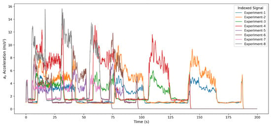
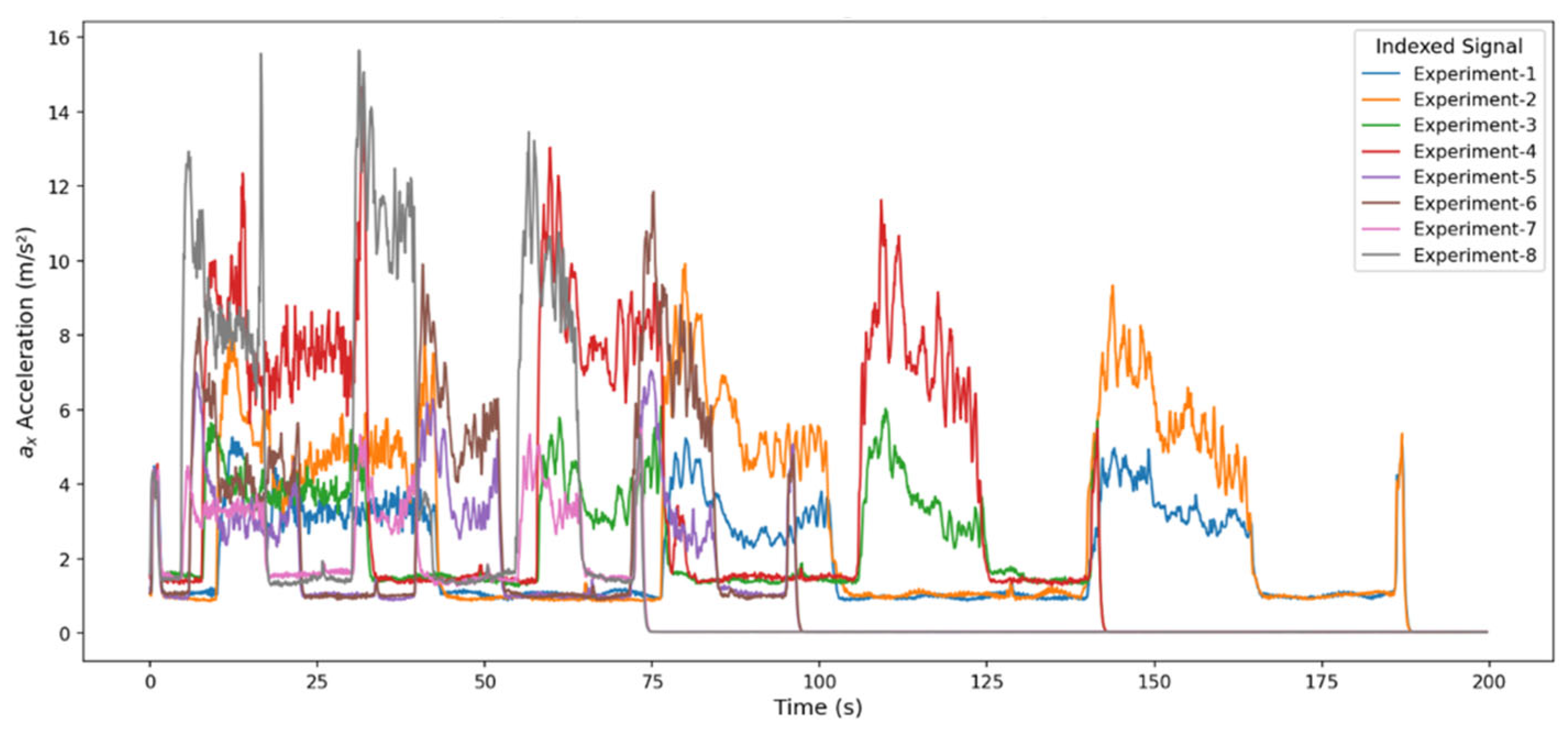
As shown in Figure 9, the superimposed vibration signals along the ax axis indicate that the main cutting force is concentrated here and reveal three distinct, repeating acceleration bands that match the cutting steps in all experiments. The variation in amplitude across experiments shows that the system’s dynamic energy increases sharply with higher feed rate (f), depth of cut (ap), and rotational speed (n). For example, high-parameter experiments (f = 0.10 mm/rev, ap = 1.0 mm, n = 2000 rpm) produced more aggressive vibration responses, with sharp peaks of 10–15 m/s2, whereas low-parameter experiments (f = 0.05 mm/rev, ap = 0.5 mm, n = 1500 rpm) showed lower amplitude and a more stable profile. Across all signals, there is a sudden acceleration rise at transitions, plateau behavior during cutting, and rapid damping after, indicating that the ax axis precisely reflects cutting force changes.
Figure 9.
Integrated representation of the x-axis acceleration time series obtained from experimental setups.
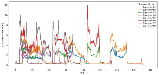
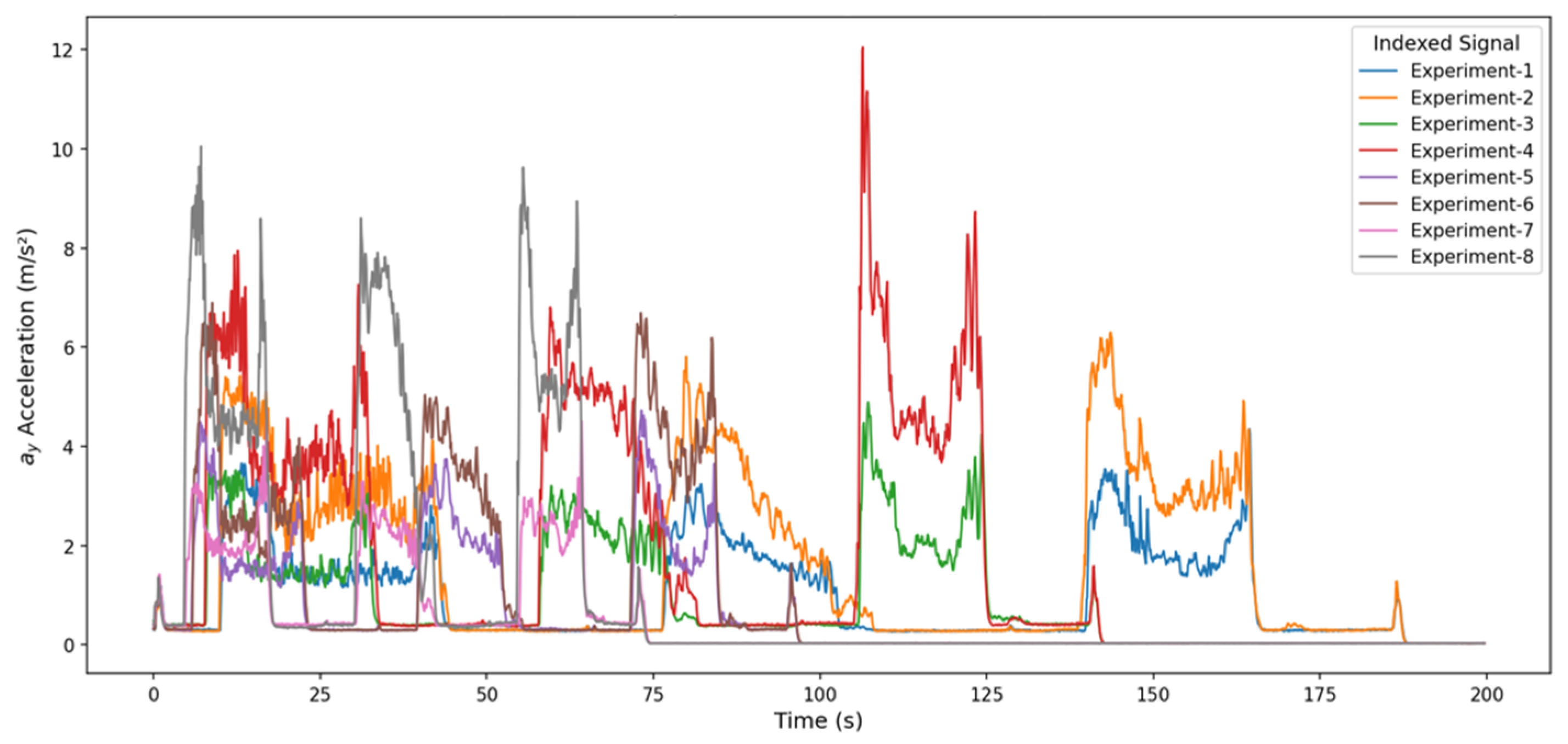
The superimposed vibration signals for the aᵧ axis, shown in Figure 10, indicate that the vertical force components have a secondary effect in the cutting process, as their amplitudes are lower than those of the ax axis. While the signals produced a significant but more limited acceleration increase in the three periodic regions corresponding to the cutting steps, this shows that vertical loads are an auxiliary vibration component rather than a dominant one in tool-workpiece interaction. Specifically, in experiments (especially 4, 6, and 8) with high feed rates and large depths of cut, the amplitudes increased significantly, with short peaks and pronounced irregularities appearing in the transition regions. Conversely, for experiments with low parameter values, the signal was more stable and had a lower amplitude. Overall, the aᵧ axis reflects elastic oscillations driven by system rigidity and vertical forces, exhibiting a dynamic response that is sensitive to increases in cutting parameters but less aggressive than that of the ax axis.
Figure 10.
Integrated representation of the y-axis acceleration time series obtained from experimental setups.
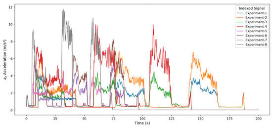
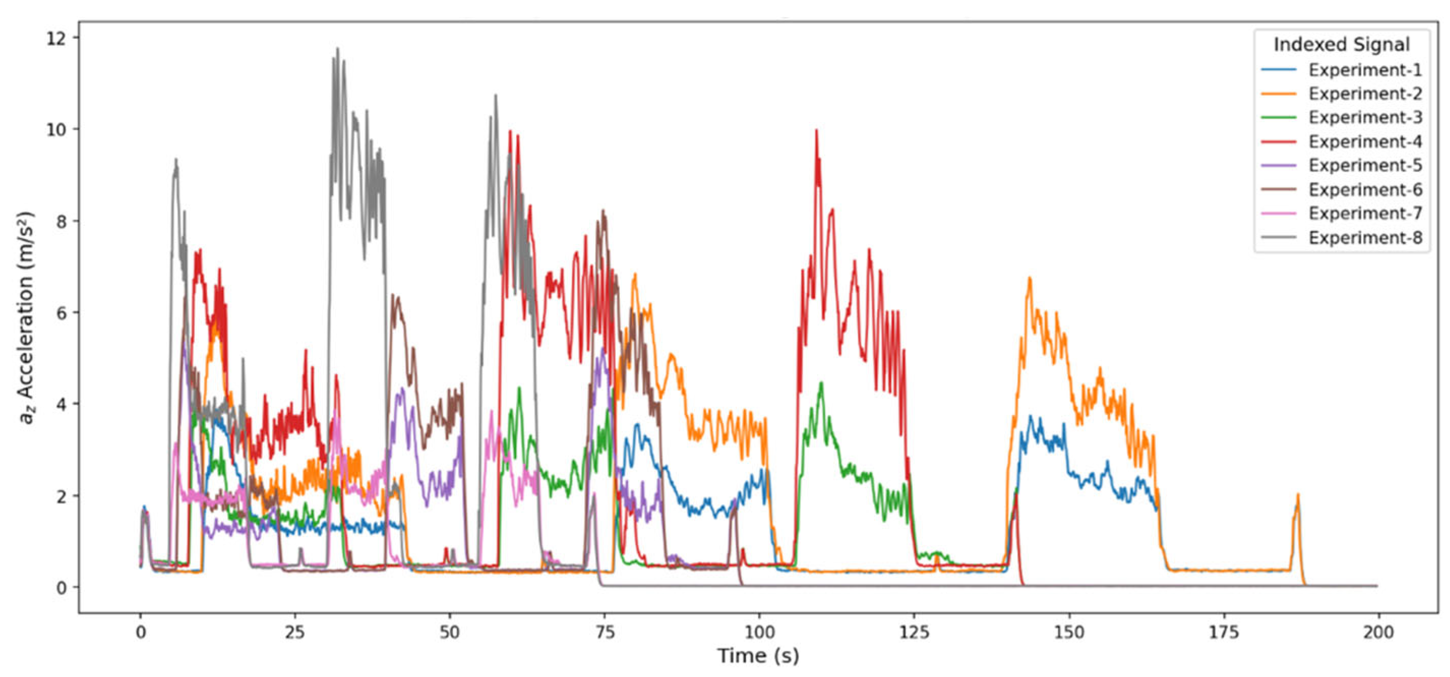
The vibration signals of the az axis shown in Figure 11 reflect the system’s dynamic rigidity, especially in the horizontal direction, as well as the horizontal components of tool-workpiece contact. The amplitude levels are lower than on the ax axis but exhibit a more regular distribution than on the aᵧ axis, indicating that the z-axis is a more stable carrier throughout the process. In experiments (4, 6, and 8) with high cutting parameters, significant amplitude increases occur, displaying sudden, short-lived jumps, especially in the second and third chip-removal zones. In contrast, experiments with low parameters produce more homogeneous signals with lower amplitudes. Generally, the signal is synchronized with the cutting steps and shows a relatively smooth profile in steady-state regimes, while local peaks of limited magnitude arise at transition moments depending on the system’s rigidity and the tool’s vibration modes. This behavior demonstrates that the az axis contributes less lateral oscillation but activates significant horizontal vibration modes as the cutting load increases. Overall, the presence of minor axial vibrations indicates the process’s horizontal stability and a moderately sensitive, yet controllable, dynamic response to increases in process parameters.
Figure 11.
Integrated representation of the z-axis acceleration time series obtained from experimental setups.
When the vibration signals obtained along the three axes (ax, ay, az) are combined, it is clear that the effect of the experimental cutting parameters on the system dynamics is consistent. The ax axis, being the dominant component of the cutting force, produced the highest amplitudes, and high vibration levels were observed, especially in experiments where the feed rate increased, despite stable regions. The ay axis represented lower-amplitude vertical force components; although the signal form was generally regular, it showed short-term fluctuations in the transition regions due to changes in the cutting direction. The az axis, on the other hand, exhibited a more stable dynamic response, reflecting the system’s horizontal rigidity, and significant amplitude increases were observed only at high cutting parameters. In all axes, characteristic vibration regions synchronized with the machining steps were clearly distinguishable, and a systematic increase in amplitude with increasing parameter values was observed across experiments.
This section provides a holistic comparison of vibration trends by superimposing acceleration signals from all experiments onto a single axis. While this multi-graph setup may appear complex, the ground truth acceleration signals for each experiment are already shown separately in Section 3.3. Thus, readers can directly compare the behaviors in the superimposed graphs with the individual experiments in that section, supporting both overall and experiment-specific analyses.
3.2. Comparing the Training Dynamics of LSTM and GRU
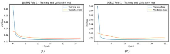
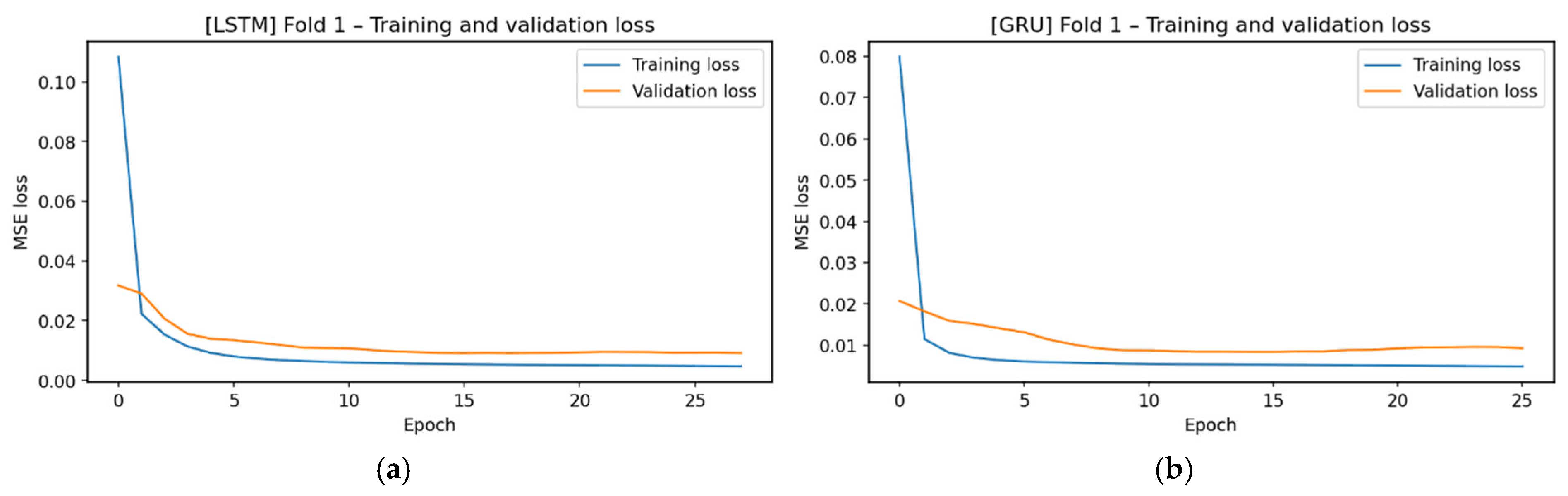
Both LSTM and GRU models exhibit rapid learning behavior in Figure 12. Training loss decreases sharply within the first few epochs, after which the training and validation curves plateau at low levels, entering a stable regime. The absence of a significant training-validation divergence between the models indicates that both models achieve stable learning without overfitting, thanks to the regular structure of the Fold-1 dataset.
Figure 12.
Training and validation loss values. (a) Loss values for Fold 1 obtained with LSTM, (b) Loss values for Fold 1 obtained with GRU.
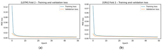
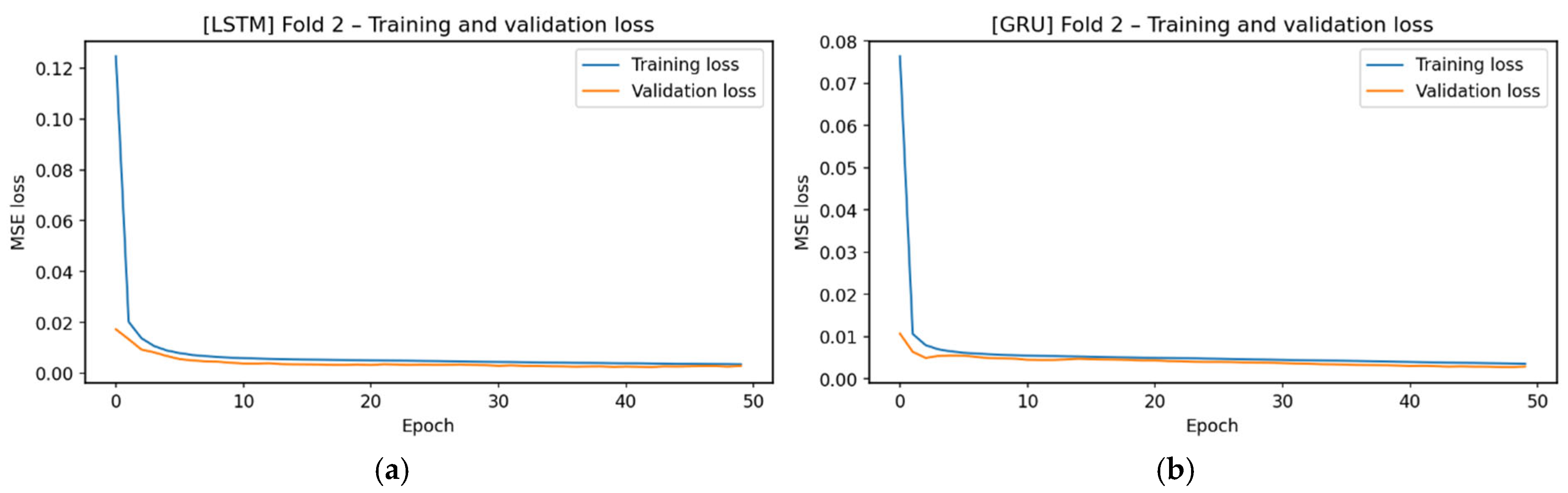
The training and validation loss curves for Figure 12 show rapid model convergence. LSTM and GRU significantly reduced losses in the first few epochs, reaching a low-level plateau region in approximately 5–10 epochs. The similarity between the training and validation losses indicates that the models successfully learned the Figure 13 dataset without overfitting.
Figure 13.
Training and validation loss values. (a) Loss values for Fold 2 obtained with LSTM, (b) Loss values for Fold 2 obtained with GRU.
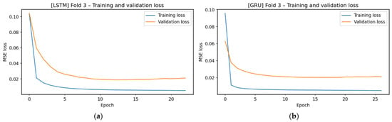
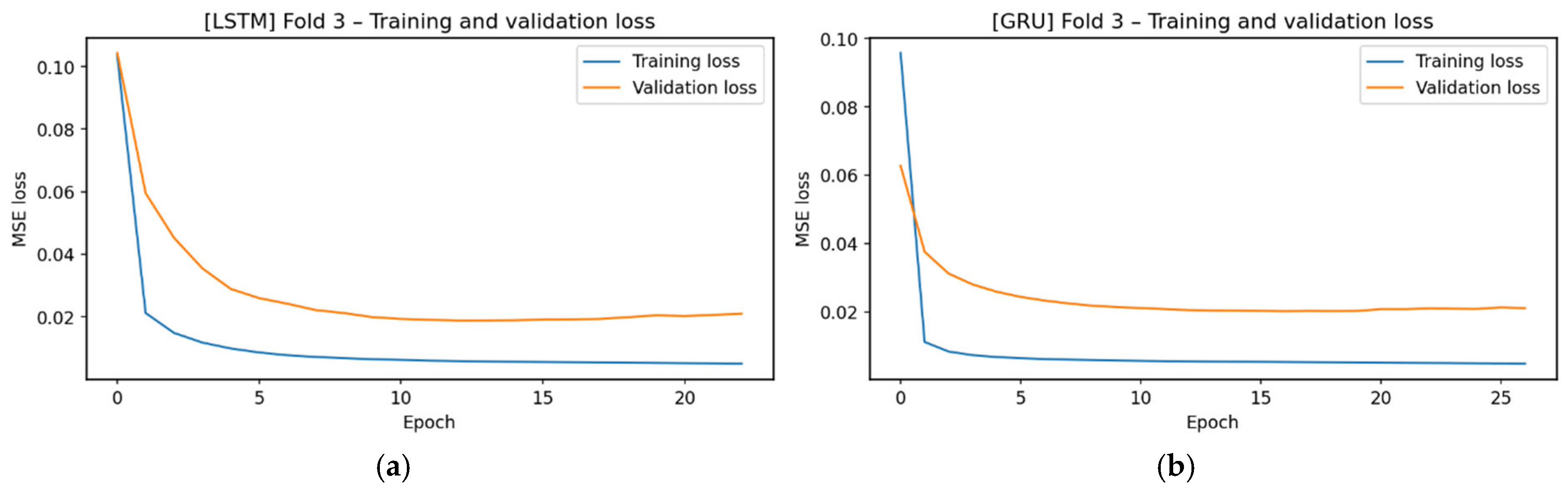
The results in Figure 14 show that LSTM and GRU converge regularly. Initial losses are lower than in Figure 13. Both models steadily decrease training and validation losses. Validation loss is higher than in earlier Folds. The wider gap between their training and validation losses indicates that the Fold-3 dataset is more predictable and easier for the models to generalize to.
Figure 14.
Training and validation loss values. (a) Loss values for Fold 3 obtained with LSTM, (b) Loss values for Fold 3 obtained with GRU.
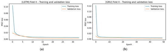
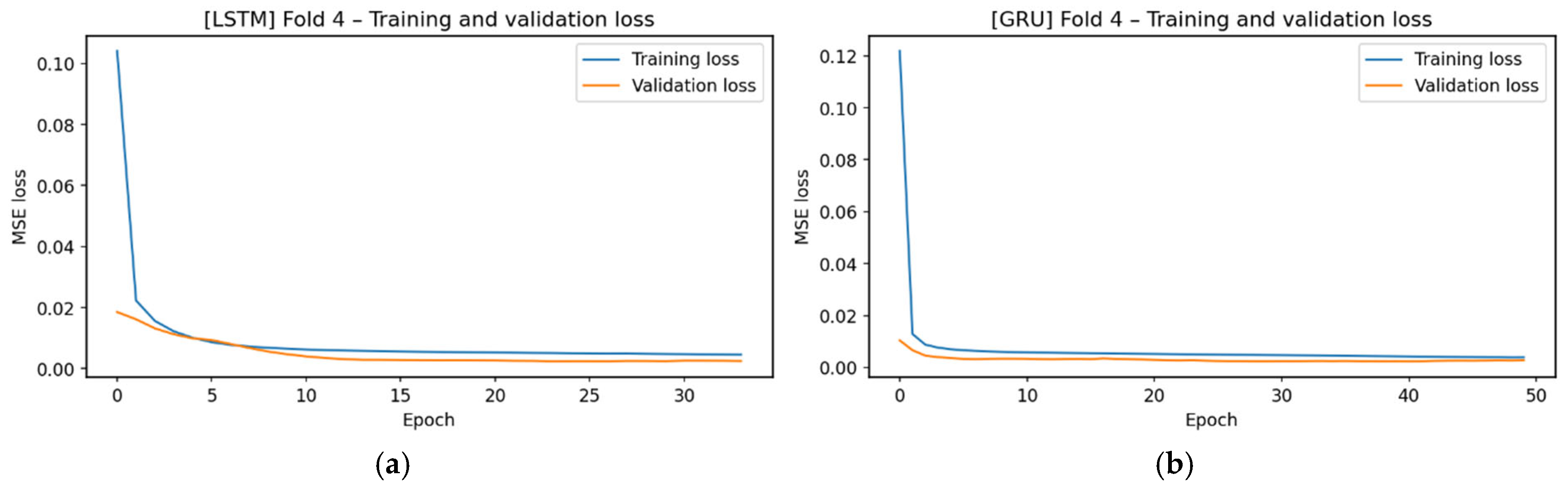
Figure 15 is one of the scenarios with the highest initial losses among all folds. Despite high initial losses, LSTM and GRU experienced a rapid decline in the first epochs, and after the first few epochs, the training and validation curves settled into a plateau region at low levels, quite close to each other. Both models achieved a stable overall error profile for this fold, performing a learning process that avoided the risk of overfitting.
Figure 15.
Training and validation loss values. (a) Loss values for Fold 4 obtained with LSTM, (b) Loss values for Fold 4 obtained with GRU.
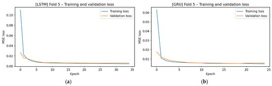
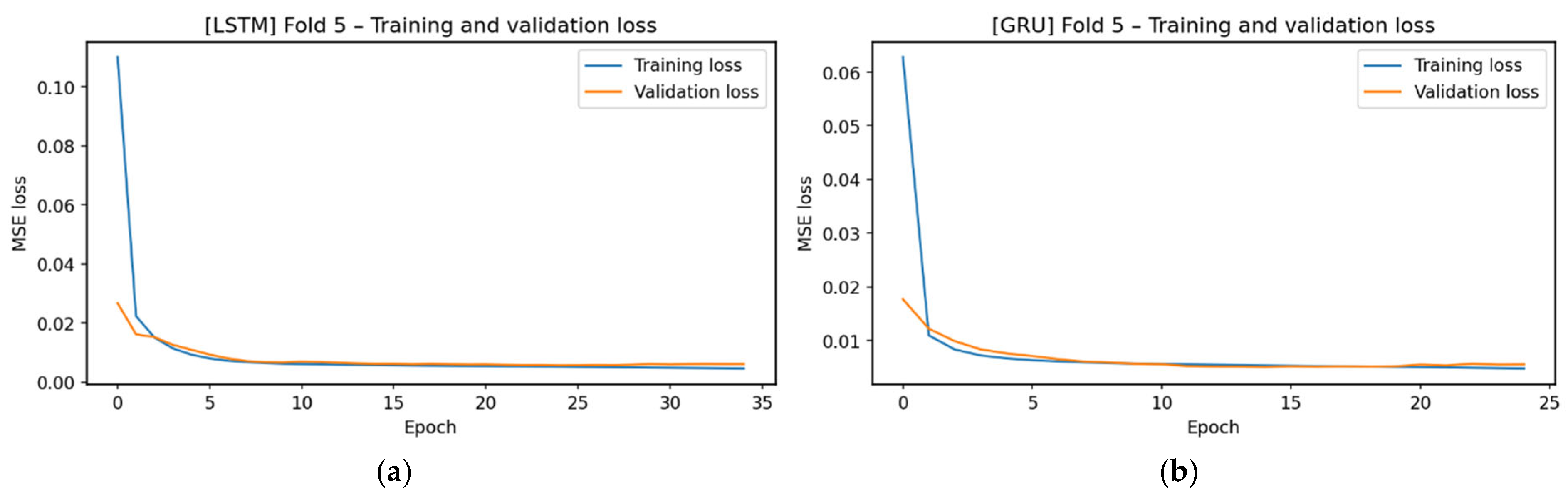
The loss curves for Figure 16 indicate a predictable pattern in the dataset. Both training and validation losses are low, leading to rapid convergence and nearly identical curves. This shows models learn Fold-5 with little error.
Figure 16.
Training and validation loss values. (a) Loss values for Fold 5 obtained with LSTM, (b) Loss values for Fold 5 obtained with GRU.
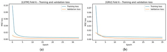
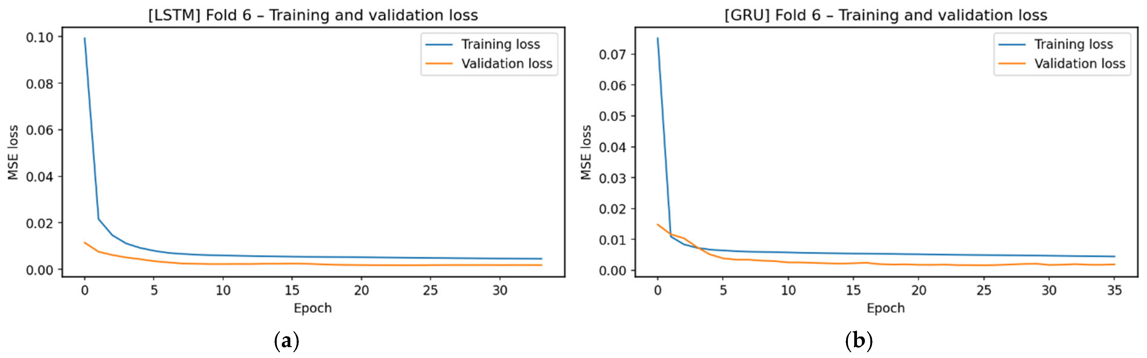
In Figure 17, the loss curves of LSTM and GRU show a similar trend, with both models quickly reaching the low-loss region. The very close progression of the LSTM and GRU curves indicates that this fold exhibits a regular vibrational structure and does not hinder the models’ generalization performance. The observed low and stable loss profile confirms that Fold-6 is learned steadily by the models.
Figure 17.
Training and validation loss values. (a) Loss values for Fold 6 obtained with LSTM, (b) Loss values for Fold 6 obtained with GRU.
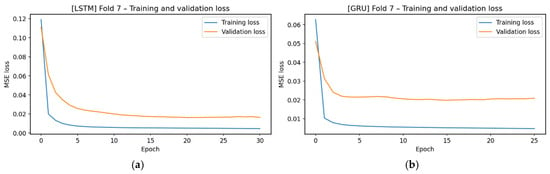
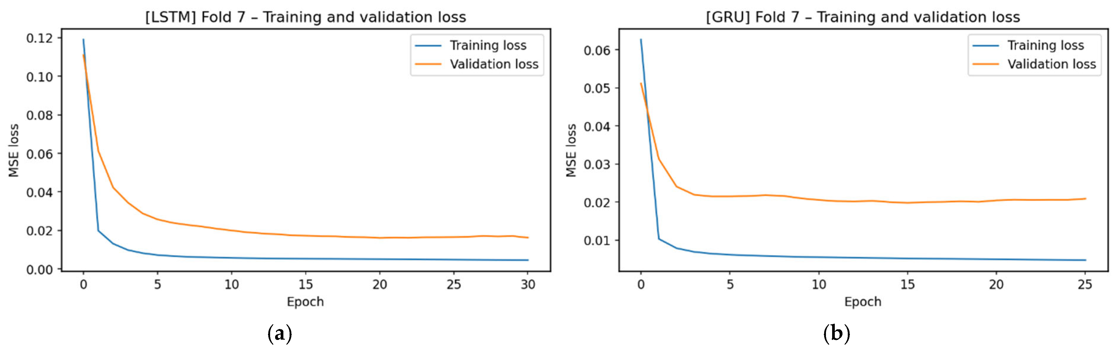
In the Figure 18 loss graphs, the training loss rapidly decreased to very low levels. The validation loss decreased more slowly and plateaued. Although the gap between the training and validation curves was larger, both settled at low levels. This suggests that Fold-7 data has a regular structure with small, unlearnable local variations. Still, the validation losses remain low, and models converge stably without overfitting.
Figure 18.
Training and validation loss values. (a) Loss values for Fold 7 obtained with LSTM, (b) Loss values for Fold 7 obtained with GRU.
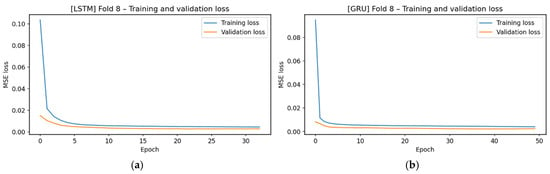
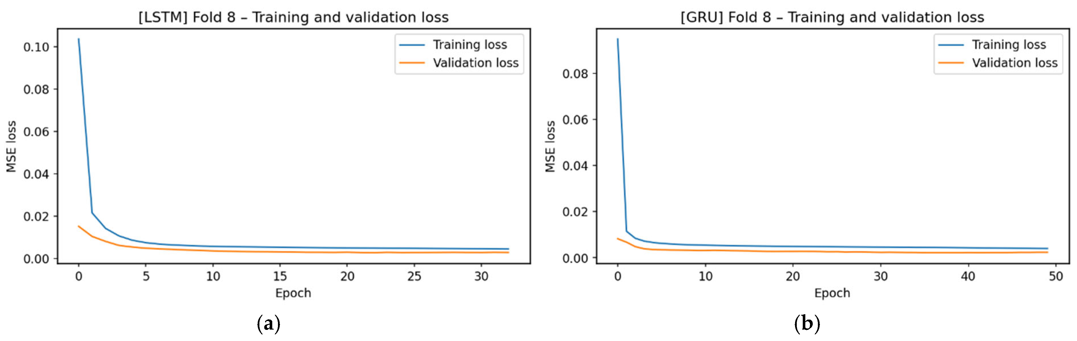
In Figure 19, both LSTM and GRU models quickly converge and plateau at low levels. The narrow gap between training and validation curves shows this fold maintains regular oscillations and does not challenge the models’ generalization. The curves indicate that Fold-8 data is highly learnable with minimal risk of overfitting.
Figure 19.
Training and validation loss values. (a) Loss values for Fold 8 obtained with LSTM, (b) Loss values for Fold 8 obtained with GRU.
When all folds are examined, LSTM and GRU models generally converge rapidly and reach stable plateaus at low levels. Training and validation losses in Fold-1, Fold-2, Fold-5, Fold-6, and Fold-8 progressed similarly, suggesting consistent vibrational patterns and effective model learning without overfitting. In Fold-3 and Fold-7, validation losses exceeded the training curves, but both still showed generalization capacity with stabilized losses. Fold-4 had high initial losses but quickly reached a stability comparable to that of other folds. Overall, low loss across all folds indicates that the models consistently learn distinct vibrational patterns.
3.3. Cross-Fold Analysis of LSTM-GRU Prediction Behavior
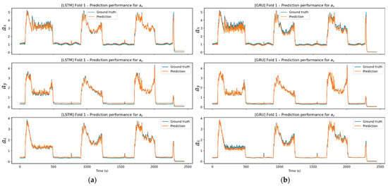
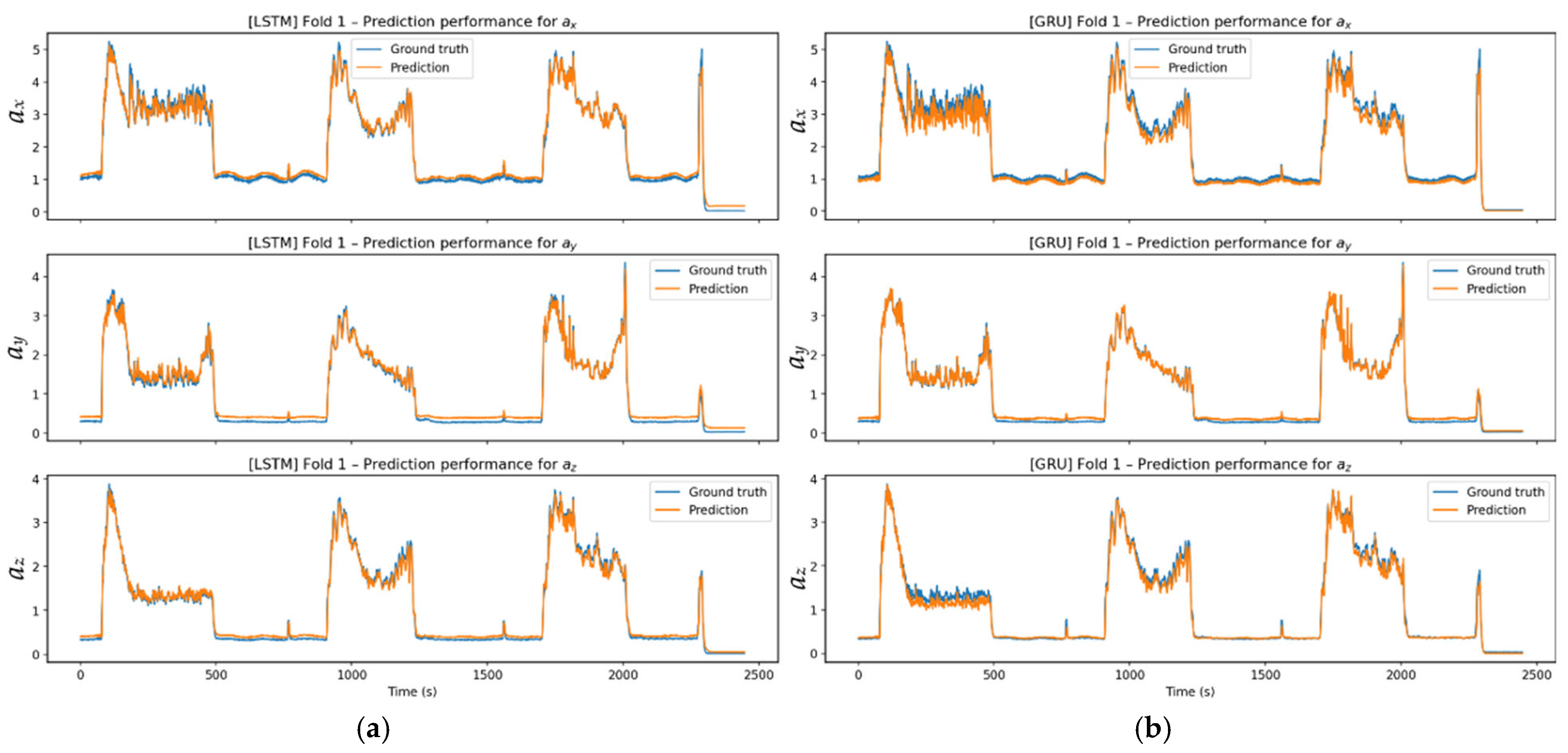
The vibration signals obtained in Fold-1, given in Figure 20, are directly related to the three successive chip removal steps (1→2→3) performed on the workpiece. The three distinct vibration regions in the time domain correspond to changes in cutting force and tool dynamic stiffness during each pass. In particular, the high amplitudes in the AX axis are consistent with dominant cutting forces and tool deflection in this direction, while the ay and az axes reflect lower lateral force components. When comparing model performances, the LSTM model produced smoother, more long-term, relationship-sensitive predictions in stable cutting regimes across all three cutting steps. In contrast, the GRU model responded faster to abrupt amplitude changes in the transition regions, closely tracking local fluctuations but introducing short-term overshoots. This faster response is attributed to the GRU model’s update gate dynamics, which enable rapid adaptation to abrupt changes but can result in small overshoot peaks. These fast update dynamics and aggressive adaptation capabilities, characteristic of RNN architectures such as GRU, are discussed in the study [34]. Despite these nuances, LSTM predictions showed better agreement with the true signal, especially in low-amplitude regions, whereas GRU exhibited more pronounced fluctuations in some local vibrational components. Nevertheless, both models successfully reproduced the macrodynamics and demonstrated strong generalization performance across the overall profile.
Figure 20.
Prediction performance: (a) Experimental and predicted values for Fold 1 using the LSTM model across all axes; (b) Experimental and predicted values for Fold 1 using the GRU model across all axes.
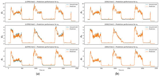
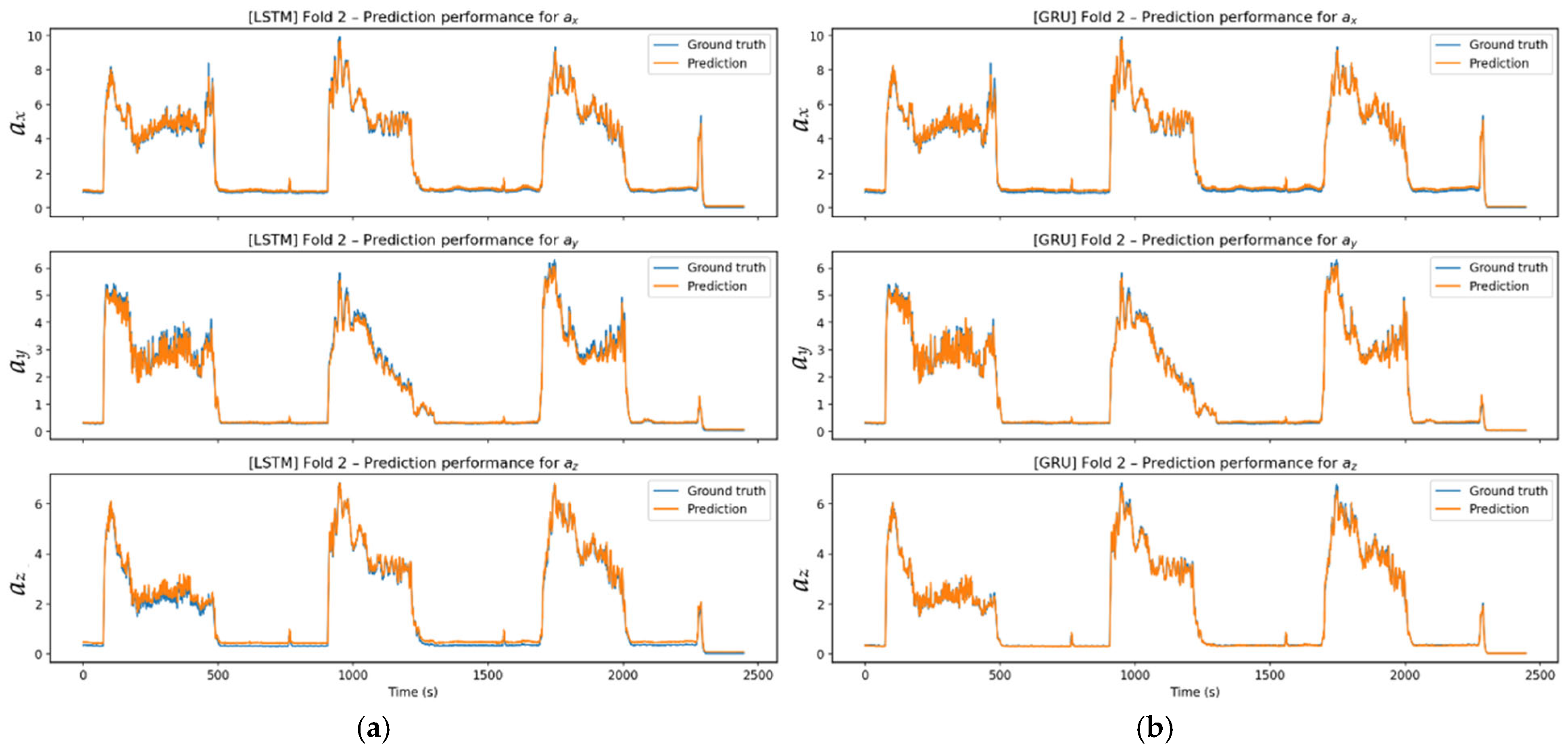
In the Figure 21 prediction results, LSTM and GRU successfully captured the overall oscillation behavior in three axes. While the models successfully tracked the true signal during rapid transitions corresponding to the cutting steps, LSTM predictions showed less ripple in the regions of abrupt rises and falls. GRU, although producing more pronounced local oscillations during transitions, accurately captured the overall trend of the signal. Both models effectively tracked amplitude changes.
Figure 21.
Prediction performance: (a) Experimental and predicted values for Fold 2 using the LSTM model across all axes; (b) Experimental and predicted values for Fold 2 using the GRU model across all axes.
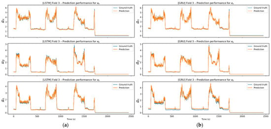
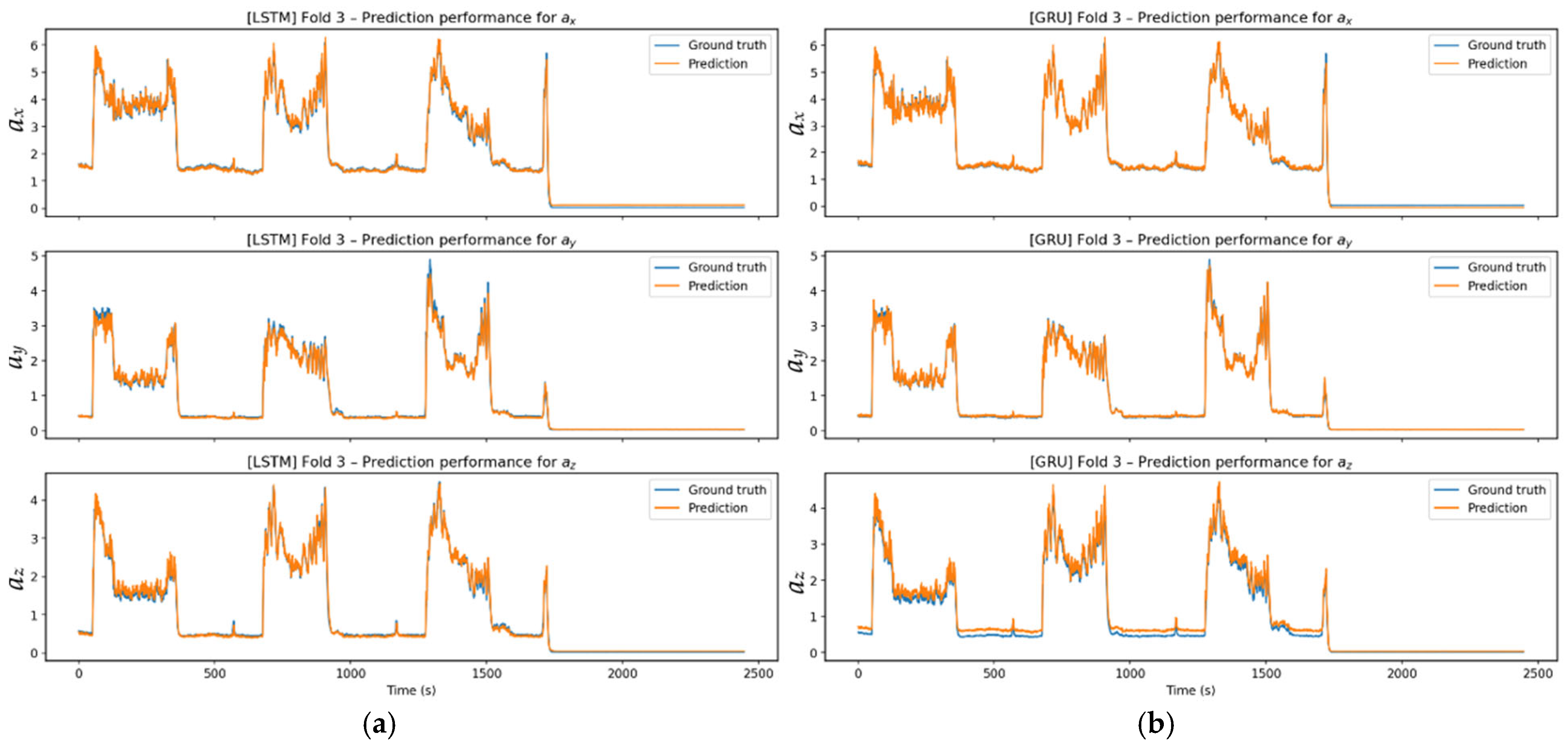
Figure 22 prediction charts show that the models successfully capture trends, stable areas, and transition points in the signal. Compared to LSTM, which provides a smoother prediction line, GRU is more responsive to sudden changes and reacts more strongly to short peaks.
Figure 22.
Prediction performance: (a) Experimental and predicted values for Fold 3 using the LSTM model across all axes; (b) experimental and predicted values for Fold 3 using the GRU model across all axes.
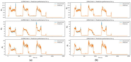
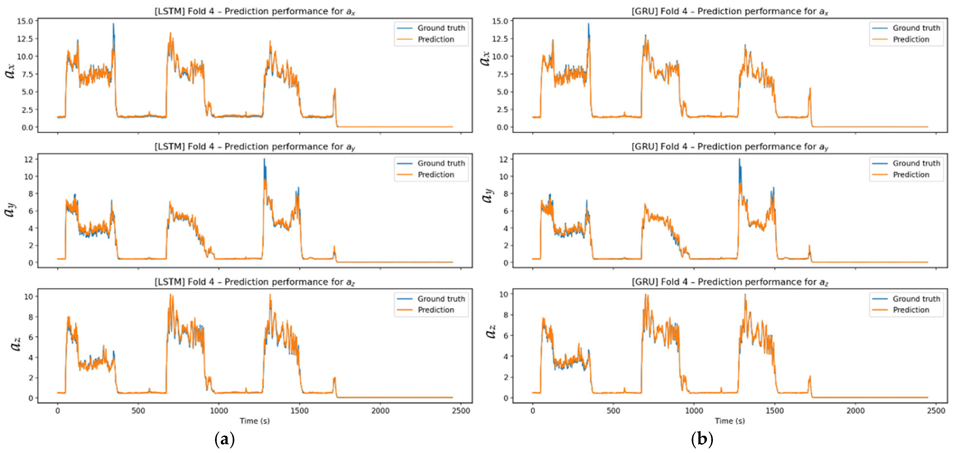
The Figure 23 signals are more challenging to model because they exhibit irregular and high-amplitude variations. GRU responds quickly to abrupt spikes, occasionally producing short-term overshoots. LSTM, however, tracks the overall signal with a smoother profile.
Figure 23.
Prediction performance: (a) Experimental and predicted values for Fold 4 using the LSTM model across all axes; (b) experimental and predicted values for Fold 4 using the GRU model across all axes.
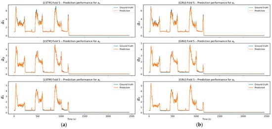
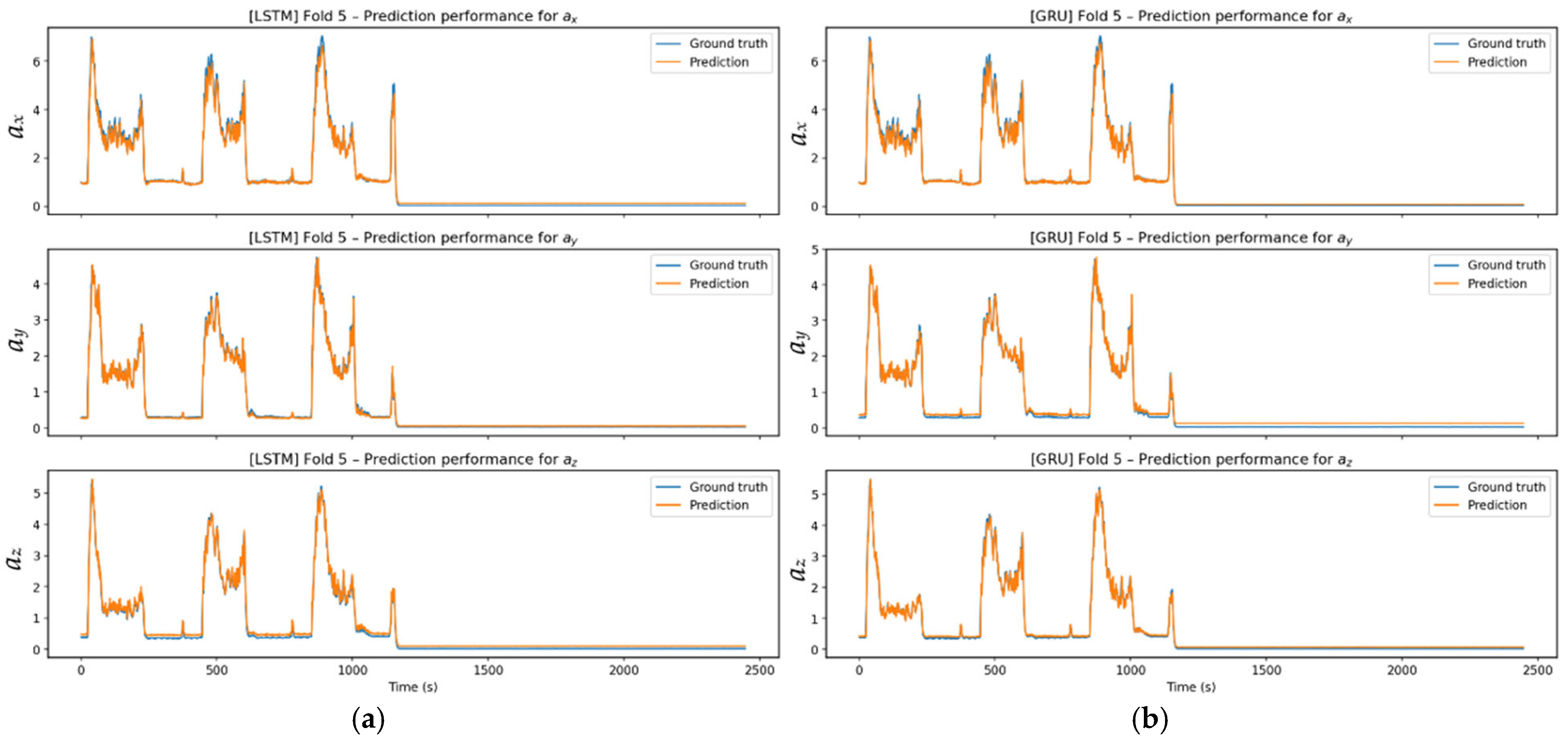
Figure 24 prediction results show that both models accurately track the vibration profile across three axes. LSTM excels at following long-term stable regions, while GRU is more responsive to local fluctuations. The regular structure of the Fold-5 dataset enables both models to deliver stable, reliable predictions across low-amplitude stable and high-amplitude cutoff zones.
Figure 24.
Prediction performance: (a) Experimental and predicted values for Fold 5 using the LSTM model across all axes; (b) experimental and predicted values for Fold 5 using the GRU model across all axes.
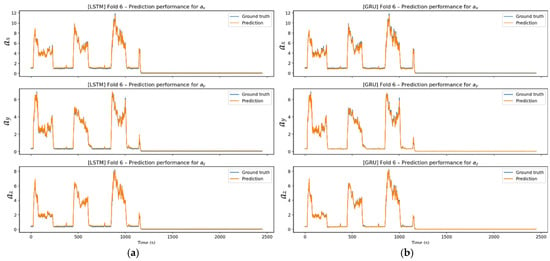
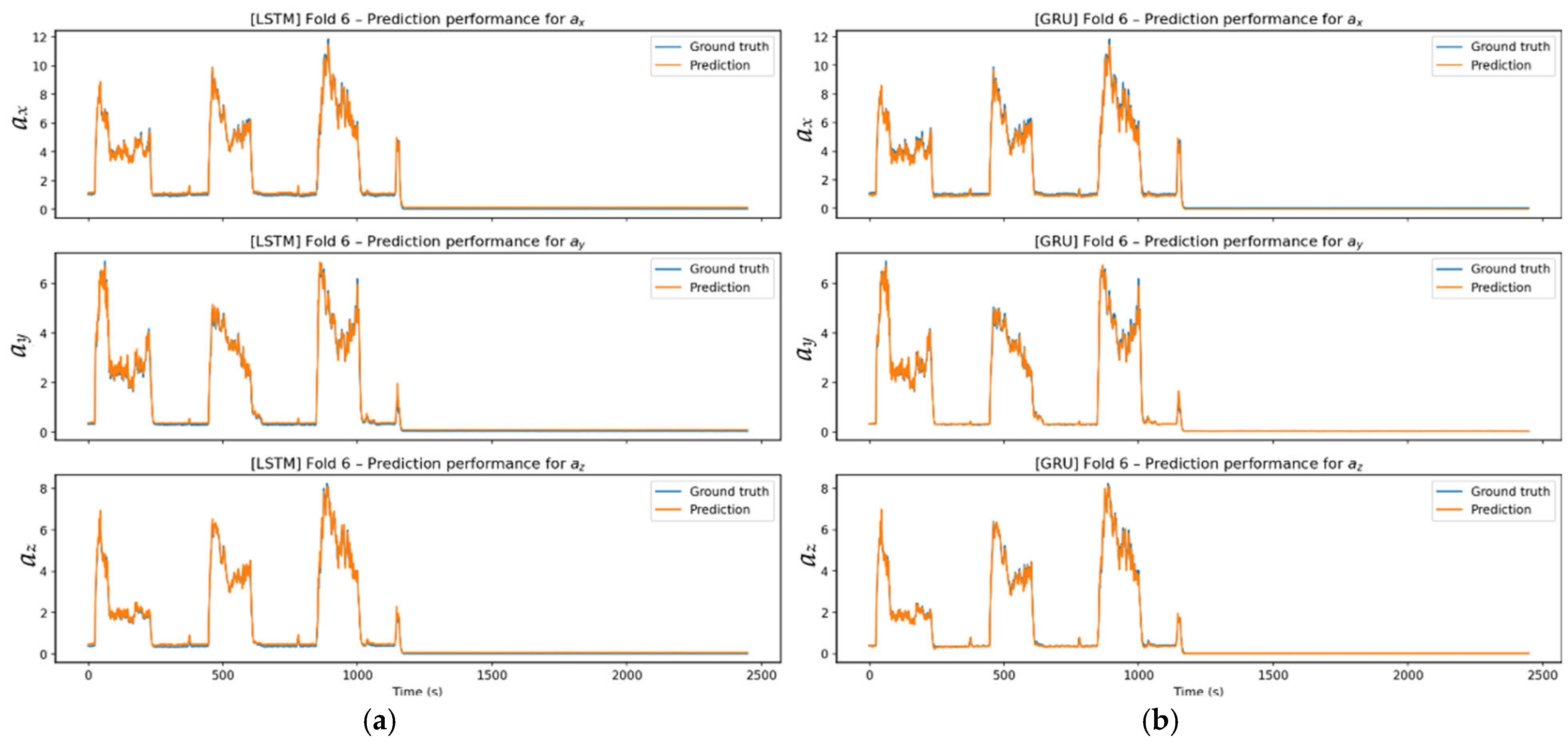
The Figure 25 signal exhibits a stable structure, as reflected in the model’s performance. Both LSTM and GRU capture the signal trend and axis-based amplitude variations with high accuracy, with the prediction and actual signals almost coinciding in most regions. Thanks to the regular, iterable structure of Fold-6, the models demonstrate strong generalization performance and exhibit stable predictions along the axes.
Figure 25.
Prediction performance: (a) Experimental and predicted values for Fold 6 using the LSTM model across all axes; (b) experimental and predicted values for Fold 6 using the GRU model across all axes.
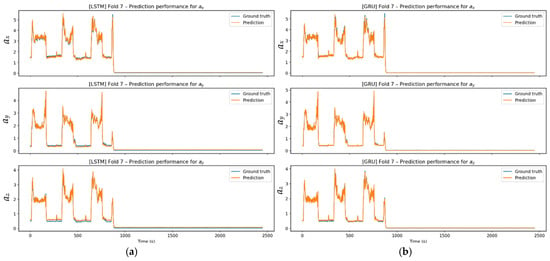
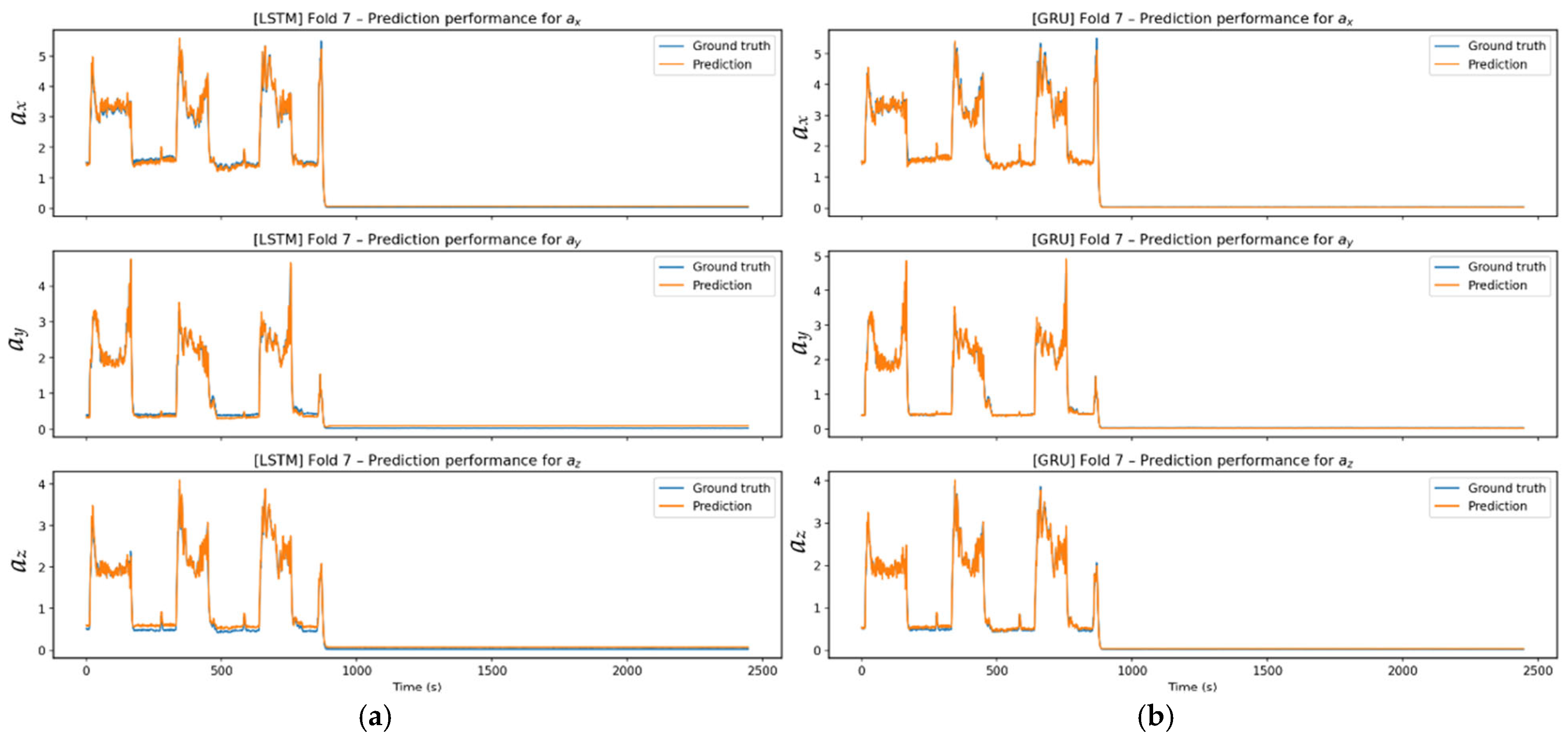
The Figure 26 prediction performance graphs indicate that both models track the signal with high accuracy. LSTM delivers relatively smooth predictions in stable regions, showing steady performance. In contrast, GRU demonstrates more pronounced oscillations, especially in transition and high-amplitude regions. As Fold-7 is typically a predictable signal, both models have low error levels despite these behavioral differences.
Figure 26.
Prediction performance: (a) Experimental and predicted values for Fold 7 using the LSTM model across all axes; (b) experimental and predicted values for Fold 7 using the GRU model across all axes.
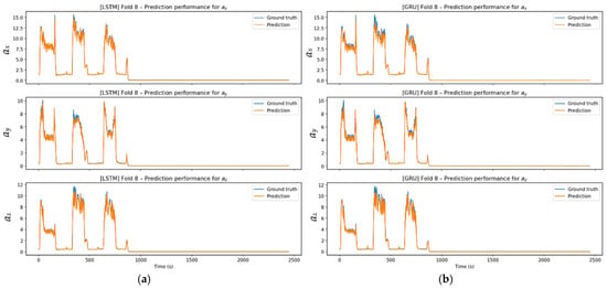
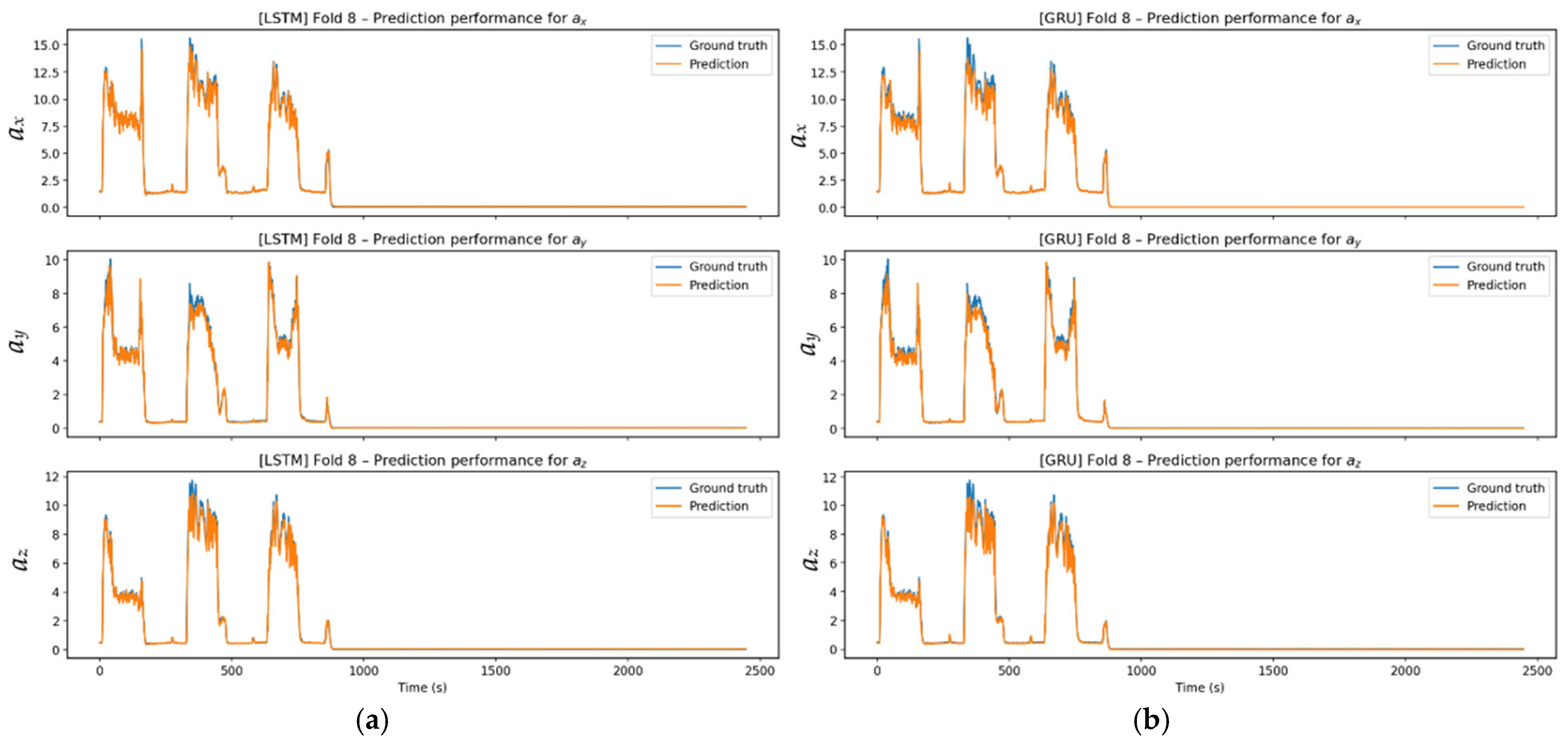
In Figure 27, LSTM and GRU models successfully reproduced the signal structure, including high-amplitude oscillatory steps, across all three axes. While LSTM predictions showed high overlap with the actual signal in transition and stable regions, GRU predictions showed limited local fluctuations at transition points. Nevertheless, both models consistently captured the abrupt acceleration changes corresponding to the cutting steps, the overall form of the signal, and its periodic behavior. Both models effectively capture the macrodynamics of the signal.
Figure 27.
Prediction performance: (a) Experimental and predicted values for Fold 8 using the LSTM model across all axes; (b) experimental and predicted values for Fold 8 using the GRU model across all axes.
Considering all folds, both LSTM and GRU models reproduced the fundamental dynamics of vibration signals with high accuracy. LSTM offered smoother, lower-ripple predictions, particularly in stable regions, as it captured long-term dependencies more consistently, while GRU responded more quickly to abrupt acceleration changes at transition moments, tracking local variations more sharply. Although this rapid adaptation led to limited overshoot in some folds, the overall trend was accurately captured. Both models performed similarly across folds with regular signal structures; however, in high-amplitude and irregular structures, LSTM showed a more stable prediction profile, while GRU showed a more reactive one. Nevertheless, in all folds, the models consistently represented the macro behavior of the signal, demonstrating strong generalization performance.
3.4. Comparative Performance of Models According to Error Criteria
The axial RMSE values in Table 8 show the difficulty levels of the folds for each model. The ax axis has the highest error for all models, while error levels are lower on the ay and az axes. For each model, Fold-7 shows the lowest error, while Fold-4 and Fold-8 show the highest.
Table 8.
Axial RMSE values according to LSTM and GRU algorithms.
Table 9 shows that Fold-7 is most successful, with the lowest RMSE and MAE. Fold-4 and Fold-8 have higher errors due to more complex dynamics. All R2 values are above 0.98, indicating the models explain the variance with high accuracy.
Table 9.
Average error values according to LSTM and GRU algorithms.
Table 10 shows that LSTM and GRU achieve closely comparable overall prediction performance, indicating that neither architecture provides a clear overall advantage in terms of predictive accuracy. LSTM yields a marginally lower mean RMSE and slightly higher mean R2, whereas GRU achieves a lower mean MAE and slightly lower RMSE values along the ay and az axes. The principal observation is therefore not the superiority of one model over the other, but their comparable generalization performance combined with different error-response characteristics. This is also consistent with the time-history comparisons, where LSTM generally provides smoother predictions, while GRU responds more strongly to short-duration variations and abrupt changes.
Table 10.
Comparison of average performance of LSTM and GRU algorithms.
Analyzing all folds together reveals that both LSTM and GRU models can accurately model the vibration signals obtained under different cutting conditions. Training and validation losses vary across folds in their initial values and convergence rates. However, all models show a rapid decline, followed by a stable plateau in later epochs. This confirms that the networks learn the signal dynamics effectively and enter a stable learning regime without overfitting. Fold-based analyses showed that, in scenarios with more regular signals (e.g., Fold-5 and Fold-7), losses converge faster and prediction errors are significantly reduced. Conversely, error levels increase in folds with irregular or transition-weighted signals (e.g., Fold-4 and Fold-8). R2 values above 0.98 across all folds show that the models explain a large portion of the variance and maintain consistent prediction performance. Axial estimation results also support these findings. Both models successfully capture the signal’s fundamental amplitude and transition characteristics across three axes. LSTM and GRU loss curves converge rapidly in the first few epochs across folds. This quick convergence is due to the models’ ability to learn fundamental dynamic dependencies, enabled by the iterative nature of vibration signals. The curves plateau early, indicating that no new information will be learned in later epochs, and parameter optimization is complete. This shows that the dataset’s complexity matches the model’s capacity, so the model does not overfit and achieves optimal performance with minimal computational cost. Overall, LSTM produces smoother and more stable predictions, while GRU is more reactive and responds faster to abrupt changes. The performance difference is limited, and both models reliably model the temporal dynamics of vibration signals produced during CNC milling.
3.5. Benchmark Comparison with Additional Trainable Models
To enable a comprehensive algorithmic comparison, additional trainable benchmark models were implemented and evaluated alongside the primary LSTM and GRU architectures. These additional models comprised MLP, 1D-CNN, and Transformer Encoder architectures, which represent non-recurrent, convolutional, and attention-based learning approaches, respectively. The previously reported LSTM and GRU results were maintained as the primary recurrent model outcomes, and the additional benchmark models were assessed using the same LOEO validation protocol. The overall benchmark results are summarized in Table 11.
Table 11.
Performance results of additional trainable benchmark models.
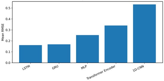
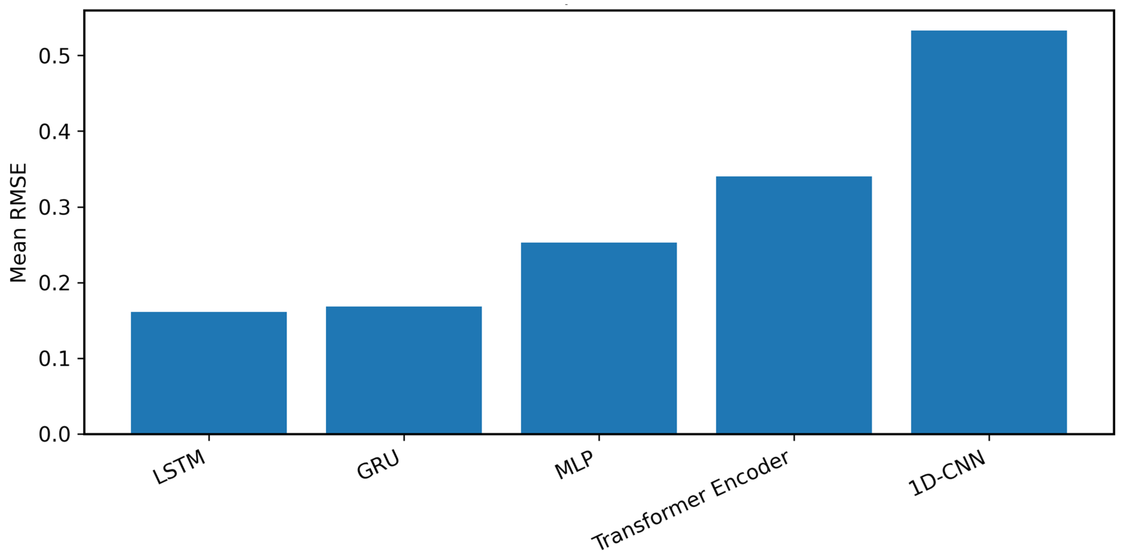
The benchmark results show that recurrent architectures provided the strongest prediction performance among the evaluated trainable models. As shown in Table 10, Table 11, and Figure 28, the LSTM and GRU models achieved lower mean RMSE values than the additional MLP, Transformer Encoder, and 1D-CNN benchmark models. Among the additional benchmark models, MLP achieved lower average RMSE values than the 1D-CNN and Transformer Encoder models. These findings indicate that gated recurrent architectures are better suited for modeling the process-level multi-axis acceleration response considered in this study.
Figure 28.
Mean RMSE comparison of the main recurrent models and additional trainable benchmark models.
4. Discussion
When the vibration characteristics were examined, it was observed that the acceleration amplitudes measured in the tool holder region increased significantly with increasing spindle speed. In contrast, due to shorter machining time, the tool holder region was subjected to higher-amplitude dynamic loads for a shorter period. Increasing the depth of cut increased cutting forces across all operating conditions, leading to higher vibration amplitudes. Reducing the feed rate by half, on the other hand, increased the machining time, causing the tool holder region to be under dynamic load for a longer period and increasing the regional acceleration levels. Performance analysis of deep learning-based models shows that LSTM and GRU architectures produce stable, consistent predictions across different cutting conditions. Comparison of RMSE, MAE, and R2 metrics revealed that the LSTM model offers more stable learning and generalization performance, especially in vibration signals involving long-term dynamics. In contrast, the GRU model performed competitively in regions characterized by abrupt, transient dynamic changes, thanks to its faster adaptation. These findings, obtained under a LOEO-based validation strategy, demonstrate that the proposed approach can be reliably generalized under varying machining conditions. Statistical analysis further characterized the predictive performance of the LSTM and GRU models across the eight LOEO folds. The mean ± standard deviation values were 0.15997 ± 0.06253 and 0.16106 ± 0.06823 for RMSE, 0.10008 ± 0.02538 and 0.08992 ± 0.02583 for MAE, and 0.99107 ± 0.00195 and 0.99085 ± 0.00325 for R2 for LSTM and GRU, respectively. A two-sided paired Wilcoxon signed-rank test yielded p-values of 0.8438 for RMSE, 0.1953 for MAE, and 0.9453 for R2, further supporting the closely comparable performance profiles of the two recurrent architectures across the evaluated folds. The benchmark comparison also provided additional quantitative evidence: based on the average RMSE of LSTM and GRU (0.1605), the recurrent models achieved approximately 36.4%, 52.8%, and 69.9% lower RMSE than MLP, Transformer Encoder, and 1D-CNN, respectively. These findings provide statistical and quantitative support for the robustness of the recurrent modeling framework and its strong predictive performance under the adopted evaluation conditions. In this respect, the study provides a generalizable, applicable framework for data-driven modeling of vibrations in CNC milling processes. The additional benchmark evaluation demonstrated that, compared with non-recurrent, convolutional, and attention-based trainable models, the LSTM and GRU architectures provided more consistent and accurate predictions, thereby supporting the main recurrent modeling framework adopted in this study. The temporal resolution of the exported dataset should also be considered when interpreting the present results. Since the prediction framework operates on time-history records separated by approximately 0.08 s, the analysis is primarily directed toward process-level temporal acceleration variations rather than detailed spectral characterization of spindle harmonics, tooth-passing components, structural modes, or chatter phenomena. Therefore, the present dataset is not intended for spectral characterization of spindle harmonics, tooth-passing frequencies, structural modes, or chatter bands. Future research could extend the proposed framework by using higher-frequency raw acceleration measurements to investigate frequency-domain milling dynamics and chatter-related phenomena, while also considering higher depth-of-cut levels, particularly for Al6061, and different cutting-tool geometries and configurations to further evaluate acceleration-response behavior and model performance under more diverse machining conditions.
5. Conclusions
This study investigated deep learning-based time series approaches to model real-time vibration behavior in the tool holder region during CNC milling. In experimental studies conducted on Al-6061 material, spindle speeds were set at 1500 and 2000 rpm, feed rates at 0.05 and 0.1 mm/rev, and depth of cut at 0.5 mm and 1 mm. The experimental data and model prediction results obtained under the determined milling conditions were comprehensively evaluated.
The key findings showed that both LSTM and GRU provided high and closely comparable predictive performance across unseen experimental runs under the LOEO framework, while both recurrent architectures outperformed the MLP, Transformer Encoder, and 1D-CNN benchmark models. Overall, the results support the effectiveness of recurrent time-series modeling for multi-axis acceleration-response prediction within the investigated CNC milling parameter space.
Funding
This research received no external funding.
Data Availability Statement
The data supporting the findings of this study were obtained experimentally and are available from the author upon reasonable request.
Acknowledgments
During the preparation of this manuscript, the author used ChatGPT (GPT-6 Astra Max) for English-language polishing, grammatical correction, and wording refinement. The author subsequently reviewed and revised the text and takes full responsibility for the content of the manuscript.
Conflicts of Interest
The author declares no conflict of interest.
References
- Ford, D.G.; Myers, A.; Haase, F.; Lockwood, S.; Longstaff, A. Active vibration control for a CNC milling machine. Proc. Inst. Mech. Eng. Part C J. Mech. Eng. Sci. 2013, 228, 230–245. [Google Scholar] [CrossRef] [Scilit]
- Li, B.; Li, L.; He, H.; Mao, X.; Jiang, X.; Peng, Y. Research on modal analysis method of CNC machine tool based on operational impact excitation. Int. J. Adv. Manuf. Technol. 2019, 103, 1155–1174. [Google Scholar] [CrossRef] [Scilit]
- Yesilyurt, I.; Ozturk, H. Tool condition monitoring in milling using vibration analysis. Int. J. Prod. Res. 2007, 45, 1013–1028. [Google Scholar] [CrossRef] [Scilit]
- Bhogal, S.S.; Sindhu, C.; Dhami, S.S.; Pabla, B.S. Minimization of surface roughness and tool vibration in CNC milling operation. J. Optim. 2015, 2015, 192030. [Google Scholar] [CrossRef] [Scilit]
- Shihan, M.; Chandradass, J.; Kannan, T.T.M. Investigation of vibration analysis during end milling process of monel alloy. Mater. Today Proc. 2021, 39, 695–699. [Google Scholar] [CrossRef] [Scilit]
- Wszołek, G.; Czop, P.; Słoniewski, J.; Dogrusoz, H. Vibration monitoring of CNC machinery using MEMS sensors. J. Vibroengineering 2020, 22, 735–750. [Google Scholar] [CrossRef] [Scilit]
- Wang, H.; Huang, Z.; Wang, C. Design of Vibration Test System for CNC Milling Machine. In Proceedings of the 2020 2nd International Conference on Big Data and Artificial Intelligence; Association for Computing Machinery: New York, NY, USA, 2021; pp. 279–284. [Google Scholar] [CrossRef] [Scilit]
- Uwajambo, P.; Thakur, N. Numerical and Experimental Modal Analysis of CNC Machine. Master’s Thesis, Blekinge Institute of Technology, Karlskrona, Sweden, June 2021. [Google Scholar]
- Chen, C.C.; Liu, N.M.; Chiang, K.T.; Chen, H.L. Experimental investigation of tool vibration and surface roughness in the precision end-milling process using the singular spectrum analysis. Int. J. Adv. Manuf. Technol. 2012, 63, 797–815. [Google Scholar] [CrossRef] [Scilit]
- Mohd Ghazali, M.H.; Rahiman, W. Vibration analysis for machine monitoring and diagnosis: A systematic review. Shock Vib. 2021, 2021, 9469318. [Google Scholar] [CrossRef] [Scilit]
- Umamaheswara Raju, R.S.; Ravi Kumar, K.; Vargish, K.; Bharath Kumar, M. Machine learning based surface roughness assessment via CNC spindle bearing vibration. Int. J. Interact. Des. Manuf. 2025, 19, 477–494. [Google Scholar] [CrossRef] [Scilit]
- Karabacak, Y.E. Deep learning-based CNC milling tool wear stage estimation with multi-signal analysis. Eksploat. Niezawodn. Maint. Reliab. 2023, 25, 168082. [Google Scholar] [CrossRef] [Scilit]
- Kaliyannan, D.; Thangamuthu, M.; Pradeep, P.; Gnansekaran, S.; Rakkiyannan, J.; Pramanik, A. Tool condition monitoring in the milling process using deep learning and reinforcement learning. J. Sens. Actuator Netw. 2024, 13, 42. [Google Scholar] [CrossRef] [Scilit]
- Tambake, N.; Deshmukh, B.; Pardeshi, S.; Salunkhe, S.; Cep, R.; Nasr, E.A. Fault diagnosis of a CNC hobbing cutter through machine learning using three axis vibration data. Heliyon 2025, 11, e41637. [Google Scholar] [CrossRef] [Scilit]
- Iqbal, M.; Madan, A.K.; Ahmad, N. Vibration and acoustic signal-based bearing fault diagnosis in CNC machine using an improved deep learning. Iran J. Comput. Sci. 2024, 7, 723–733. [Google Scholar] [CrossRef] [Scilit]
- Oleaga, I.; Pardo, C.; Zulaika, J.J.; Bustillo, A. A machine-learning based solution for chatter prediction in heavy-duty milling machines. Measurement 2018, 128, 34–44. [Google Scholar] [CrossRef] [Scilit]
- Gao, Y.; Qiu, T.; Song, C.; Ma, S.; Liu, Z.; Liang, Z.; Wang, X. Vibration signal–based surface roughness prediction with hybrid kernel extreme learning machine for robotic face milling. Int. J. Adv. Manuf. Technol. 2025, 139, 5137–5151. [Google Scholar] [CrossRef] [Scilit]
- Finkeldey, F.; Wöste, F.; Werner, D.; Schönecker, R.; Biermann, D.; Wiederkehr, P. Cluster-based prediction of chatter vibrations in milling operations. Procedia CIRP 2025, 133, 388–393. [Google Scholar] [CrossRef] [Scilit]
- Vinchon, G.; Knittel, D.; Nouari, M.; Makich, H.; Yakob, A.; Romani, D. Vibration based milling diagnostics using artificial intelligence. In Surveillance, Vibrations, Shock and Noise; Institut Supérieur de l’Aéronautique et de l’Espace: Toulouse, France, 2023. [Google Scholar]
- Shah, M.; Vakharia, V.; Chaudhari, R.; Vora, J.; Pimenov, D.Y.; Giasin, K. Tool wear prediction in face milling of stainless steel using singular generative adversarial network and LSTM deep learning models. Int. J. Adv. Manuf. Technol. 2022, 121, 723–736. [Google Scholar] [CrossRef] [Scilit]
- Hu, L.; Gao, R.; Guo, Y.B. Time-Series Data-Driven Machine Learning of Milling Chattering. J. Manuf. Sci. Eng. 2025, 147, 101005. [Google Scholar] [CrossRef] [Scilit]
- Li, E.; Zhou, J.; Yang, C.; Wang, M.; Li, Z.; Zhang, H.; Jiang, T. CNN-GRU network-based force prediction approach for variable working condition milling clamping points of deformable parts. Int. J. Adv. Manuf. Technol. 2022, 119, 7843–7863. [Google Scholar] [CrossRef] [Scilit]
- Eski, İ. Vibration analysis of drilling machine using proposed artificial neural network predictors. J. Mech. Sci. Technol. 2012, 26, 3037–3046. [Google Scholar] [CrossRef] [Scilit]
- Esim, E.; Yıldırım, Ş. Drilling performance analysis of drill column machine using proposed neural networks. Neural Comput. Appl. 2017, 28, 79–90. [Google Scholar] [CrossRef] [Scilit]
- Çetinkaya, M.B.; Esim, E.; İşci, M. Analysis of the vibration characteristic of an experimental turning lathe using artificial neural networks. Arab. J. Sci. Eng. 2021, 46, 2597–2611. [Google Scholar] [CrossRef] [Scilit]
- Xu, Z.; Zhang, B.; Li, D.; Yip, W.S.; To, S. Digital-twin-driven intelligent tracking error compensation of ultra-precision machining. Mech. Syst. Signal Process. 2021, 219, 111630. [Google Scholar] [CrossRef] [Scilit]
- Liu, Y.; Shu, Y.; Xu, Z.; Han, S.; Zhang, C.; Chen, M. One-dimensional convolutional neural network model driven intelligent operation phases identification of hydraulic press using energy data. Eng. Appl. Artif. Intell. 2025, 155, 111079. [Google Scholar] [CrossRef] [Scilit]
- Yin, S.; Liu, X.; Xu, Z.; Li, Z.; Zhang, H.; Wang, H.; Kang, R. Establishment of microstructure prediction model for ultrasonic vibration machining of tungsten heavy alloy based on continuum mechanics. Mater. Des. 2026, 116374. [Google Scholar] [CrossRef] [Scilit]
- Yin, S.; Liu, M.; Tian, Y.; Li, F.; Li, G.; Kang, R. Research on sensitivity of strain rate in ultrasonic elliptical vibration cutting of tungsten alloys. J. Mater. Res. Technol. 2025, 267, 3594–3607. [Google Scholar] [CrossRef] [Scilit]
- He, J.; Meng, X.; Guo, J.; Li, F.; Zhao, J.; Jin, X.; Liu, Y. Cross-condition tool wear prediction via feature decoupling and domain-adaptive representation learning. Mech. Syst. Signal Process. 2026, 259, 114783. [Google Scholar] [CrossRef] [Scilit]
- Rumelhart, D.E.; Hinton, G.E.; Williams, R.J. Learning representations by back-propagating errors. Nature 1986, 323, 533–536. [Google Scholar] [CrossRef] [Scilit]
- Kiranyaz, S.; Avci, O.; Abdeljaber, O.; Ince, T.; Gabbouj, M.; Inman, D.J. 1D convolutional neural networks and applications: A survey. Mech. Syst. Signal Process. 2021, 151, 107398. [Google Scholar] [CrossRef] [Scilit]
- Vaswani, A.; Shazeer, N.; Parmar, N.; Uszkoreit, J.; Jones, L.; Gomez, A.N. Attention is all you need. Adv. Neural Inf. Process. Syst. 2017, 30, 261–272. [Google Scholar]
- Cho, K.; Van Merriënboer, B.; Gulcehre, C.; Bahdanau, D.; Bougares, F.; Schwenk, H.; Bengio, Y. Learning phrase representations using RNN encoder-decoder for Statistical Machine Translation. arXiv 2014, arXiv:1406.1078. [Google Scholar]





Disclaimer/Publisher’s Note: The statements, opinions and data contained in all publications are solely those of the individual author(s) and contributor(s) and not of MDPI and/or the editor(s). MDPI and/or the editor(s) disclaim responsibility for any injury to people or property resulting from any ideas, methods, instructions or products referred to in the content. |
© 2026 by the author. Licensee MDPI, Basel, Switzerland. This article is an open access article distributed under the terms and conditions of the Creative Commons Attribution (CC BY) license.