Uncertainty-Decomposed Meta-Learning with Reliability-Gated Inference for Intelligent Few-Shot LiDAR Fault Classification

Abstract

Few-shot meta-learning supports rapid adaptation with limited labeled data, but remains sensitive to hyperparameters and support set quality. We propose Uncertainty-Decomposed Reliability-Gated Meta-Learning (UDRML). It selects support sets with low predictive entropy, combines diverse adapted models to estimate aleatoric and epistemic uncertainty through mutual information, and uses a reliability score to accept, flag, or reject predictions. We evaluate UDRML on cross-domain few-shot LiDAR fault classification using a synthetically augmented nuScenes dataset. At 10-shot, UDRML improves accuracy over MAML by 11.8 points. Gating provides a further 13.3-point gain on accepted predictions, while measured epistemic uncertainty is 78% lower than that of the strongest ensemble baseline, ECMP. The framework supports selective automation by accepting reliable predictions and directing uncertain cases to verification or a fallback.

1. Introduction

Autonomous driving relies on multiple sensors for perception [1]. Surveys of perception, localization, and decision-making identify sensor reliability as a continuing challenge [2,3]. Detecting sensor faults is essential because corrupted data can propagate through perception and planning [4,5]. Related equipment-level approaches include residual-based early-fault diagnosis of electric-hydraulic control systems [6] and optimal sensor placement for hydraulic fault diagnosis [7]. Sensor noise and environmental interference can mask faults, while their rarity makes representative training data difficult to obtain without fault injection or simulation [8]. The resulting class imbalance biases classifiers toward nominal operation [9]. These constraints motivate fault diagnosis methods that learn from few examples and provide calibrated confidence estimates.

Digital twins and high-fidelity simulators are commonly used to alleviate this scarcity [10], but a sim-to-real gap remains because synthetic data does not fully capture real sensor-specific noise. Meta-learning offers one way to bridge this gap [11,12]. Among optimization-based meta-learners, Model-Agnostic Meta-Learning (MAML) leverages diverse simulated tasks during meta-training to learn an initialization from which the model can adapt rapidly [13]; given a handful of labeled real samples, the learned initialization enables efficient parameter updates toward the target distribution [14,15]. Despite its effectiveness, standard MAML has two well-known limitations [16]. First, performance is sensitive to the interplay between the inner-loop adaptation rate ($\mathsf{\alpha }$) and the outer-loop meta-optimization rate ($\mathsf{\beta }$), and misconfiguration can destabilize training. Second, few-shot adaptation quality depends heavily on the support set composition during fine-tuning [17]: an ideal support set should be informative and noise-minimal [18], yet standard MAML samples it uniformly at random and exerts no explicit control over support set quality.

Recent meta-learning methods for fault diagnosis address different parts of this problem. Metric-based methods [12,15] learn discriminative embeddings but retain randomly sampled support sets. Architecture-enhanced methods [19] improve feature extraction, for example, through attention, while retaining predictions without confidence estimates. Cross-domain and cross-machine methods [14,20] address distribution shift but lack mechanisms to defer unreliable predictions. Ensemble-based meta-learning [21] reduces hyperparameter sensitivity without separating aleatoric and epistemic uncertainty. These limitations motivate UDRML’s joint treatment of support set quality and decomposed uncertainty for prediction review.

UDRML introduces a Meta-Training and Domain Adaptation (MTDA) module—a few-shot adaptation block tailored to fault classification and adapted from MAML [13]—together with mechanisms that jointly account for aleatoric and epistemic uncertainty. The contributions are: (1) an entropy-driven active sampling strategy that partitions the target-domain pool via Latin Hypercube Sampling and selects the support set with minimal predictive entropy, anchoring few-shot adaptation on high-confidence exemplars; (2) a hyper-ensemble [22] inference mechanism with mutual information-based uncertainty decomposition that aggregates $\mathrm{M}$ independently adapted models and separates total predictive uncertainty into aleatoric and epistemic components; and (3) a unified intelligent diagnostic framework that couples (1) and (2) with a reliability-aware decision gate, routing each prediction through accept, flag, or reject tiers. Section 2 reviews relevant work, Section 3 details UDRML, Section 4 and Section 5 present the experimental setup and comparative results, and Section 6 concludes.

2. Background and Related Work

Reliable fault classification in intelligent condition-monitoring applications not only requires accuracy, but well-calibrated uncertainty estimates, since downstream decisions—whether automated fallbacks or operator-in-the-loop verification—act on the predicted class. Predictive uncertainty is typically decomposed into aleatoric and epistemic components. Aleatoric uncertainty reflects irreducible stochasticity in the data—thermal noise, atmospheric interference, hardware-level limitations—and cannot be reduced by collecting more samples. Epistemic uncertainty arises from insufficient training data to constrain model parameters, is most pronounced for out-of-distribution inputs, and is in principle reducible with more diverse data.

Uncertainty estimation commonly uses Bayesian approximations or ensembles. Bayes by Backprop learns weight distributions [23], MC Dropout approximates posterior sampling [24], and VAEs provide a generative approach [25]. SVGD [26] and S²VGD [27] approximate the posterior with model particles. Deep Ensembles combine independently initialized networks [28], BatchEnsemble reduces computation through rank-one perturbations [29], and EMP/ECMP introduce diversity through selected submodules [30]. These methods do not directly address support set selection during few-shot domain adaptation.

Bayesian MAML maintains distributions over adapted parameters [31], PLATIPUS models maintain uncertainty over initializations [32], and recent methods extend uncertainty-aware few-shot learning to industrial diagnosis [33,34]. These approaches retain random support sets and do not separate uncertainty into components used for different decisions. Active learning approaches instead select samples for annotation efficiency [35]. Single-pass alternatives include Evidential Deep Learning [36] and DUQ [37], while Deep Gaussian Processes model input-dependent uncertainty through hierarchical layers [38]. To our knowledge, no prior framework combines support set curation, uncertainty decomposition, and selective prediction in one meta-learning pipeline.

UDRML uses mutual information decomposition for three reasons. First, estimated aleatoric uncertainty and epistemic disagreement inform the two weighted branches of the reliability gate; pre-adaptation predictive entropy separately guides support selection (Section 3.2 and Section 3.3.2). Second, the decomposition applies to adapted model predictions without changing meta-training, unlike variational or evidential objectives [23,36]. Third, varying ensemble settings is intended to improve uncertainty estimation beyond random initialization alone (Section 3.3.1). Table S1 compares the alternatives.

3. UDRML Framework

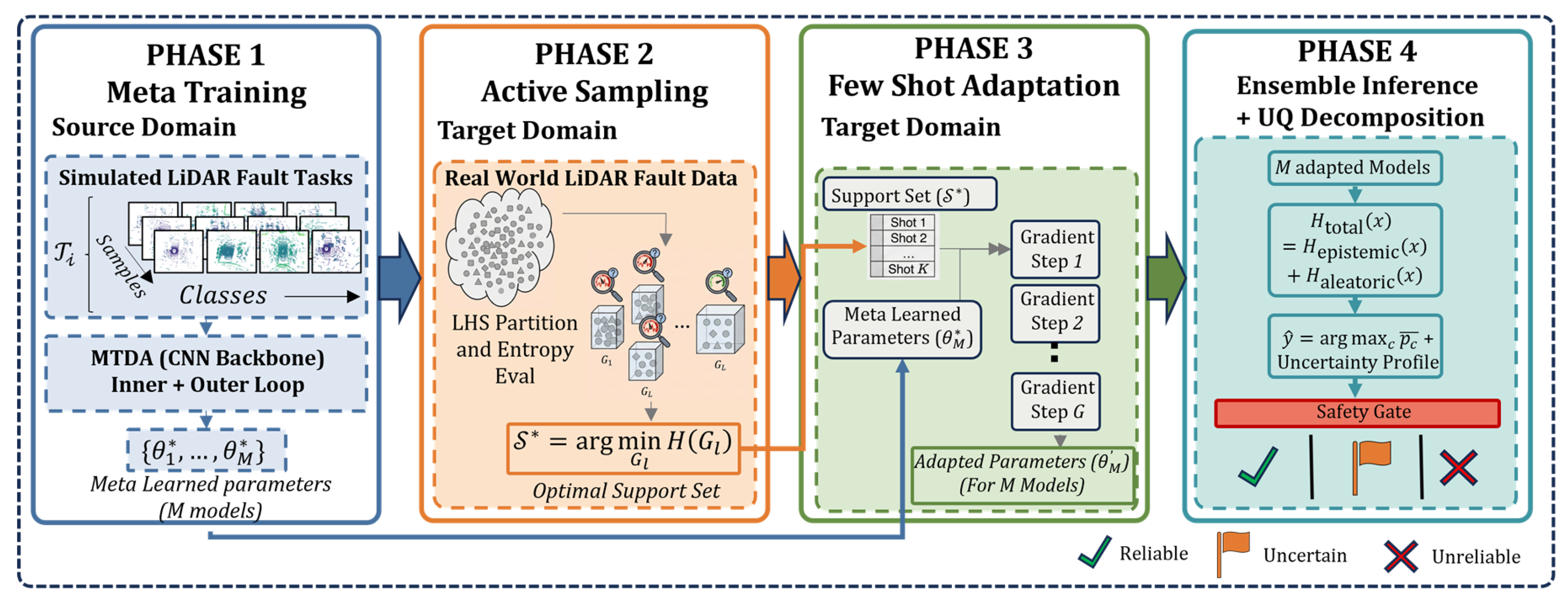
This section describes UDRML in three parts: the meta-training and adaptation algorithm (Section 3.1), the uncertainty-aware active sampling strategy (Section 3.2), and the hyper-ensemble procedure with reliability-aware decision gating (Section 3.3). An overview is shown in Figure 1.

Figure 1. Proposed UDRML framework. The superscript * denotes meta-trained parameters in θ* and the selected minimum-entropy support set in S*.

3.1. Meta-Training and Domain Adaptation (MTDA)

The MTDA module seeks an initialization $\theta \in {\mathbb{R}}^d$ that supports rapid task-specific adaptation via bi-level optimization over a task distribution $\mathrm{p}\left(\mathcal{T}\right)$. Each task ${\mathcal{T}}_{\mathrm{€}}$ is defined by a support set $S_i=\{\left(x_j,y_j\right){\}}_{j=1}^{8K}$ and a query set $Q_i=\{\left(x_j,y_j\right){\}}_{j=1}^{N_q}$, where $\mathrm{K}$ is the per-class shot count and $N_q$ is the query size.

Inner loop. For each task ${\mathcal{T}}_{\mathrm{€}}$, the support set loss is the empirical risk over $S_i$:

$${\mathcal{L}}_{{\mathcal{T}}_i}^{\mathrm{support}}\left(\theta \right)={\displaystyle \frac{1}{8K}}{\displaystyle {\sum }_{j=1}^{8K}}\mathcal{l}\left(f_{\theta }\left(x_j\right),y_j\right)$$

(1)

where $\mathcal{l}\left(\cdot ,\cdot \right)$ is the task loss (cross-entropy for classification) and $f_{\theta }$ is the base learner. The adapted parameters are obtained via gradient descent on this loss:

$${{\theta }_i}^{\prime }=\theta -\alpha \hspace{0.17em}{\nabla }_{\theta }{\mathcal{L}}_{{\mathcal{T}}_i}^{\mathrm{support}}\left(\theta \right)$$

(2)

with $\mathsf{\alpha }\in {\mathbb{R}}^{+}$ the inner-loop learning rate. Multi-step adaptation with $G$ inner gradient steps generalizes recursively as:

$${{\theta }_i}^{\prime \left(g\right)}={{\theta }_i}^{\prime (g-1)}-\alpha \hspace{0.17em}{\nabla }_{{\theta }_i{\prime }^{\left(g-1\right)}}{\mathcal{L}}_{{\mathcal{T}}_i}^{\mathrm{support}}\left({\theta }_i{\prime }^{\left(g-1\right)}\right), g=1,\dots ,G$$

(3)

with ${\theta }_i{\prime }^{\left(0\right)}=\theta$. The choice of $\alpha$ governs a bias–variance trade-off: large values risk overfitting to $S_i$, while small values yield insufficient adaptation.

Outer loop. Adapted parameters are evaluated on the query sets over a meta-batch of $N$ tasks. In contrast to standard MAML, MTDA introduces loss-proportional task weighting so that tasks with larger post-adaptation query loss exert greater influence on the meta-update. The motivation is that transfer difficulty is heterogeneous across fault categories: in our setting, fog and occlusion typically present larger sim-to-real discrepancies than sensor jitter or signal dropout. The post-adaptation query loss is:

$$L_i={\mathcal{L}}_{{\mathcal{T}}_i}^{\mathrm{query}}\left({\theta }_i\prime \right)={\displaystyle \frac{1}{N_q}}{\displaystyle {\sum }_{j=1}^{N_q}}\mathcal{l}\left(f_{{\theta }_i\prime }\left(x_j\right),y_j\right)$$

(4a)

The corresponding task weight is obtained by normalization within the current meta-batch (treated as a fixed scalar during differentiation):

$$w_i={\displaystyle \frac{L_i}{{\displaystyle {\sum }_{k=1}^N}{L}_k}}$$

(4b)

and the resulting outer-loop objective is:

$${\mathcal{L}}^{\mathrm{MTDA}}\left(\theta \right)={\displaystyle {\sum }_{i=1}^N}{w}_i\hspace{0.17em}{\mathcal{L}}_{{\mathcal{T}}_i}^{\mathrm{query}}\left({\theta }_i\prime \right)$$

(4c)

Equation (4b) gives greater weight to tasks with larger post-adaptation query losses. Uniform weights recover MAML, while assigning all weight to the highest-loss task gives a worst-case objective. Loss-proportional weighting emphasizes difficult tasks, connecting to robust optimization and hard-task mining [39] and to focal weighting of difficult examples [40]. Holding $w_i$ fixed during differentiation prevents optimization through the weights and keeps the meta-gradient a convex combination of task gradients. The meta-parameter update follows:

$$\theta \leftarrow \theta -\beta \hspace{0.17em}{\nabla }_{\theta }{\mathcal{L}}^{\mathrm{MTDA}}\left(\theta \right)$$

(5)

with $\beta$ the outer-loop learning rate. Since ${\theta }_i\prime$ depends on $\mathsf{\theta }$ through Equation (2), the gradient requires second-order differentiation:

$${\nabla }_{\theta }{\mathcal{L}}^{\mathrm{MTDA}}={\displaystyle {\sum }_{i=1}^N}{w_i\nabla }_{{\theta }_i\prime }{\mathcal{L}}_{{\mathcal{T}}_i}^{\mathrm{query}}\left({\theta }_i\prime \right)\cdot \left(I-\alpha \hspace{0.17em}{\nabla }_{\theta }^2{\mathcal{L}}_{{\mathcal{T}}_i}^{\mathrm{support}}\left(\theta \right)\right)$$

(6)

The coupled dependence on $\alpha$ and $\beta$ means suboptimal configuration of either rate can propagate instability across the bi-level optimization.

3.2. Uncertainty-Aware Active Sampling

The quality of the support set strongly influences the inner-loop optimization in Equation (2). Noisy or ambiguous samples introduce observation noise into ${\theta }_i\prime$, degrading task-specific adaptation. UDRML addresses this through an active selection strategy that selects the least uncertain exemplars. Let $D_{\mathrm{target}}=\{\left(x_j,y_j\right){\}}_{j=1}^N$ denote the available target-domain data. Using Latin Hypercube Sampling, $D_{\mathrm{target}}$ is organized as follows: K denotes the number of support samples per class; each class’s 100-sample candidate pool is partitioned into $\mathrm{L}=100/\mathrm{K}$ groups, and combining one group from each of the eight classes forms a candidate support set containing $8K$ samples: $G_1,G_2,\dots ,G_L$ with $G_l=\{\left(x_j,y_j\right){\}}_{j=1}^{8K}$. For each sample $x_j$ in a candidate group, the pre-adaptation model $f_{\theta }$ produces logits $z\in {\mathbb{R}}^C$, mapped to a predictive distribution via softmax, as shown below:

$${\pi }_c={\displaystyle \frac{exp\left(z_c\right)}{{\displaystyle {\sum }_{j=1}^C}exp\left(z_j\right)}}, c=1,\dots ,C$$

(7)

The sample-level predictive entropy, a proxy for data noise, is computed as:

$$H\left(P\right)=-{\displaystyle {\sum }_{c=1}^C}{\pi }_{c}log{\pi }_c$$

(8)

where $H\left(P\right)\in \left[0,logC\right]$, with $H\left(P\right)=0$ indicating a deterministic prediction and $H\left(P\right)=logC$ indicating maximum ambiguity. Strictly, the predictive entropy of Equation (8) is a property of the model’s predictive distribution, not of the data-generating process: for a single network it conflates irreducible observation noise with uncertainty arising from the model’s own limited knowledge, and it coincides with the true conditional entropy of the data-generating distribution only for a perfectly calibrated model [41]. We therefore employ pre-adaptation predictive entropy as an operational proxy for sample-level noise rather than as a strict aleatoric measure. This is sufficient for support set curation, which depends only on the relative ranking of candidate groups: samples whose predictions are ambiguous under the meta-trained prior, whether due to observation noise or intrinsic class overlap. These can destabilize the inner-loop gradients of Equation (2). The principled decomposition into aleatoric and epistemic components is deferred to the ensemble stage (Section 3.3.1), where it is well defined. The group-level uncertainty is the mean entropy across the $8\mathrm{K}$ samples:

$$H\left(G_l\right)={\displaystyle \frac{1}{8K}}{\displaystyle {\sum }_{j=1}^{8K}}H\left(P_j\right)$$

(9)

and the optimal support set is the candidate group with minimum aggregate uncertainty:

$$S^{\mathrm{*}}=arg\underset{G_l}{min}H\left(G_l\right)$$

(10)

so that inner-loop gradient updates in Equation (2) are anchored on lower-entropy, lower-noise samples, yielding more stable adapted parameters ${\theta }_i\prime$.

Conventional active learning selects maximum-uncertainty samples because its objective is label efficiency: uncertain samples carry the most information for an annotator. Our setting inverts the objective. Labels are already available; the support set’s role is to drive inner-loop gradient adaptation from only K samples, where a single noisy or ambiguous exemplar produces high-variance, misleading gradients [17,18]. Minimum-entropy selection therefore optimizes adaptation stability rather than annotation value. Crucially, selection operates at the group level over Latin Hypercube candidates rather than at the sample level: each candidate group inherits randomized marginal coverage of the target pool, and class balance is enforced within every group, so minimizing mean entropy chooses among diversity-preserving sets rather than trading diversity for confidence.

3.3. Hyper-Ensemble Inference and Reliability Gating

After adaptation on $S^{*}$, the ensemble estimates aleatoric and epistemic uncertainty (Section 3.3.1). The reliability gate uses these estimates to accept, flag, or reject each prediction (Section 3.3.2).

3.3.1. Hyper-Ensemble for Epistemic UQ

UDRML uses $\mathrm{M}$ independently adapted models $\{f_{{\theta }_1\prime },f_{{\theta }_2\prime },\dots ,f_{{\theta }_M\prime }\}$ with different initialization seeds, inner-loop learning rates ($\alpha$), and dropout rates (Table 1). The outer-loop rate remains $\beta =0.001$; inner learning rates range from 0.04 to 0.10 and dropout rates from 0.0 to 0.3. Following the hyper-ensemble approach [22], these settings introduce diversity beyond random initialization alone; Section 5.5 evaluates each source through ablation.

Table 1. Ensemble model configurations.

Model	Seed	α (Inner LR)	Dropout	Adaptation Rate	Regularization
M1	1	0.100	0.00	High	None
M2	2	0.080	0.10	Moderate-High	Low
M3	3	0.060	0.20	Moderate	Moderate
M4	4	0.040	0.30	Moderate-Low	Moderate-High

Each member adapts on the same curated support set, so their disagreement reflects sensitivity to the adaptation configuration. Their predictions also support the mutual information decomposition in Equations (13)–(15), whose components drive the reliability gate (Section 3.3.2). The ensemble therefore links diverse few-shot adaptation to uncertainty estimation and prediction review.

For a query sample $\mathrm{x}$, the $\mathrm{m}$-th ensemble member yields:

$$p_c^{\left(m\right)}={\displaystyle \frac{exp\left(z_c^{\left(m\right)}\right)}{{\displaystyle {\sum }_{j=1}^C}exp\left(z_j^{\left(m\right)}\right)}}, c=1,\dots ,C$$

(11)

where ${\mathrm{z}}^{\left(\mathrm{m}\right)}\in {\mathbb{R}}^{\mathrm{C}}$ are the output logits of the $\mathrm{m}$-th model. The ensemble-averaged predictive distribution is:

$${\overline{p}}_c={\displaystyle \frac{1}{M}}{\displaystyle {\sum }_{m=1}^M}{p}_c^{\left(m\right)}$$

(12)

We use a mutual information-based decomposition to disentangle epistemic from aleatoric uncertainty. The total predictive uncertainty is captured by the entropy of the mean distribution,

$$H\left[y|x\right]=-{\displaystyle {\sum }_{c=1}^C}{\overline{p}}_{c}log{\overline{p}}_c$$

(13)

which conflates both uncertainty types. The aleatoric component, representing irreducible data-level noise, is isolated as the expected entropy within individual ensemble members,

$$H_{\mathrm{aleatoric}}\left(x\right)={\displaystyle \frac{1}{M}}{\displaystyle {\sum }_{m=1}^M}\left(-{\displaystyle {\sum }_{c=1}^C}{p}_c^{\left(m\right)}log{p}_c^{\left(m\right)}\right)$$

(14)

Each member’s entropy reflects uncertainty that persists regardless of model diversity and therefore provides a model-relative estimate of noise intrinsic to the data. The epistemic component, capturing inter-model disagreement attributable to insufficient knowledge, is then obtained as the mutual information between the prediction $\mathrm{y}$ and the model parameters $\mathsf{\theta }$:

$$I\left[y;\theta |x\right]=H\left[y|x\right]-H_{\mathrm{aleatoric}}\left(x\right)$$

(15)

where $I\left[y;\theta |x\right]\in \left[0,H\left[y|x\right]\right]$. When all ensemble members agree, individual entropies approach the total entropy and $I\approx 0$, indicating low epistemic uncertainty; high mutual information signals substantial model disagreement, suggesting that the input lies in a region where the model lacks sufficient knowledge for a consistent prediction. The decomposition of Equations (13)–(15) follows the information-theoretic formulation of predictive uncertainty [42,43], in which the total entropy of the ensemble mean prediction separates into the expected member entropy (Equation (14)) and the mutual information between prediction and model parameters (Equation (15)). Under this formulation, the expected entropy term is a Bayesian estimate of aleatoric uncertainty (the uncertainty that remains, on average, once a model is fixed), with the hyper-ensemble members acting as approximate posterior samples. Two caveats bound this interpretation. First, a finite ensemble covers a limited region of parameter space, so Equation (14) approximates rather than equals the expected entropy under the true posterior. Second, even in the infinite-ensemble limit, the expected member entropy equals the genuine data-generating conditional entropy only for well-specified, calibrated members; systematic miscalibration inflates the estimate [41,44]. The improved calibration of the hyper-ensemble (Section 5.3) mitigates but does not eliminate this gap, and we accordingly interpret the aleatoric component throughout as a model-relative estimate of irreducible ambiguity rather than a measurement of the data-generating noise itself. The final prediction is obtained from the ensemble mean,

$$\widehat{y}=arg\underset{c}{max}{\overline{p}}_c$$

(16)

with $\overline{p}$ serving as the output distribution. The decomposition provides a per-prediction uncertainty profile: $H\left[y|x\right]$ quantifies total confidence, $H_{\mathrm{aleatoric}}$ flags inherently ambiguous inputs, and $I\left[y;\theta |x\right]$ indicates where additional data or model capacity could reduce uncertainty. Note that ${\mathrm{H}}_{\mathrm{aleatoric}}$ provides a post-adaptation, ensemble-level estimate of data noise that complements the pre-adaptation entropy-based sample selection in Section 3.2: the former assesses residual data ambiguity at inference, while the latter filters it during support set construction.

3.3.2. Reliability-Aware Decision Gate

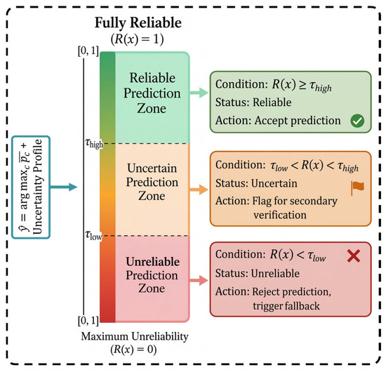
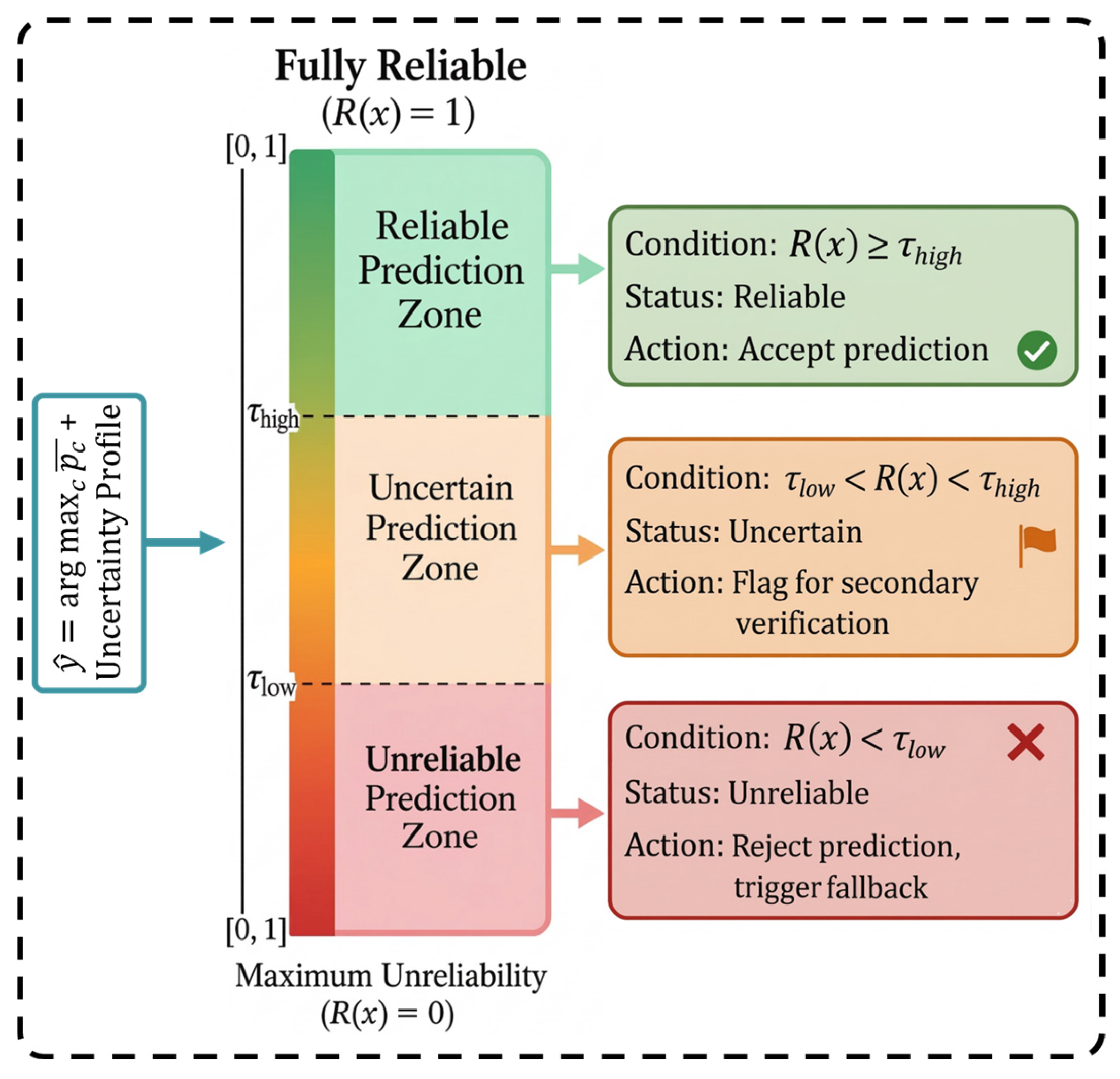
The decision gate (Figure 2) combines normalized aleatoric and epistemic uncertainty into a reliability score:

$$R\left(x\right)=1-\left[{\lambda }_1\cdot {\widehat{H}}_{\mathrm{aleatoric}}\left(x\right)+{\lambda }_2\cdot {\widehat{I}}_{\mathrm{epistemic}}\left(x\right)\right]$$

(17)

where ${\widehat{H}}_{\mathrm{aleatoric}}=H_{\mathrm{aleatoric}}/log\left(C\right)$ and ${\widehat{I}}_{\mathrm{epistemic}}=I_{\mathrm{epistemic}}/log\left(C\right)$ are scaled to $\left[\mathrm{0,1}\right]$, and ${\lambda }_1+{\lambda }_2=1$ controls relative sensitivity to data noise versus model disagreement. Predictions are routed through a three-tier structure: $R\left(x\right)\ge {\tau }_{\mathrm{high}}$ accepts the classification; ${\tau }_{\mathrm{low}}\le R\left(x\right)<{\tau }_{\mathrm{high}}$ flags it for secondary verification; and $R\left(x\right)<{\tau }_{\mathrm{low}}$ rejects it and triggers a fallback. Thresholds ${\tau }_{\mathrm{high}}$ and ${\tau }_{\mathrm{low}}$ are derived from the validation distribution of $R\left(x\right)$ at the 75th and 25th percentiles. The default weighting ${\lambda }_1={\lambda }_2=0.5$ provides a neutral starting point; in deployment these weights can be tuned, with larger ${\lambda }_1$ in noise-dominated environments and larger ${\lambda }_2$ when robustness to novel fault conditions is the priority.

Figure 2. Decision gate.

We refer to the classification pipeline (active sampling + hyper-ensemble) as UDRML, and the full framework, including the gate, as UDRML+. To ensure fair comparison over identical test distributions, all baseline comparisons in Section 5 use UDRML; the gate is evaluated separately in Section 5.5.

3.4. Procedure Summary

The full UDRML procedure comprises four phases corresponding to the modules in Section 3.1, Section 3.2 and Section 3.3. Phases 1 and 3 dominate the meta-training and adaptation cost, requiring $M\times G$ backward passes per task. Phase 2 (active sampling) requires $8\times L\times K$ forward passes from a single pre-adaptation model, since all $M$ initializations share the same meta-training distribution and their pre-adaptation uncertainties are highly correlated. Phase 4 requires $M$ forward passes per query at inference. With the configuration used in this work ($M=4$, $G=5$, $L=100/K=10$ at 10-shot), the framework remains tractable on a single GPU while still providing the diversity needed for the uncertainty decomposition in Equations (13)–(15). A fully expanded pseudocode listing, including per-line updates and the reliability gate branching, is provided in the Supplementary Materials (Algorithm S1).

4. Dataset and Experimental Setup

Experiments were conducted on a workstation with a 2.59 GHz Intel Xeon w7-3445, 64 GB RAM, and an NVIDIA RTX A4000 GPU (16 GB VRAM) (HP, Palo Alto, CA, USA), using PyTorch 2.10 with CUDA 12.6 on Windows.

4.1. Dataset

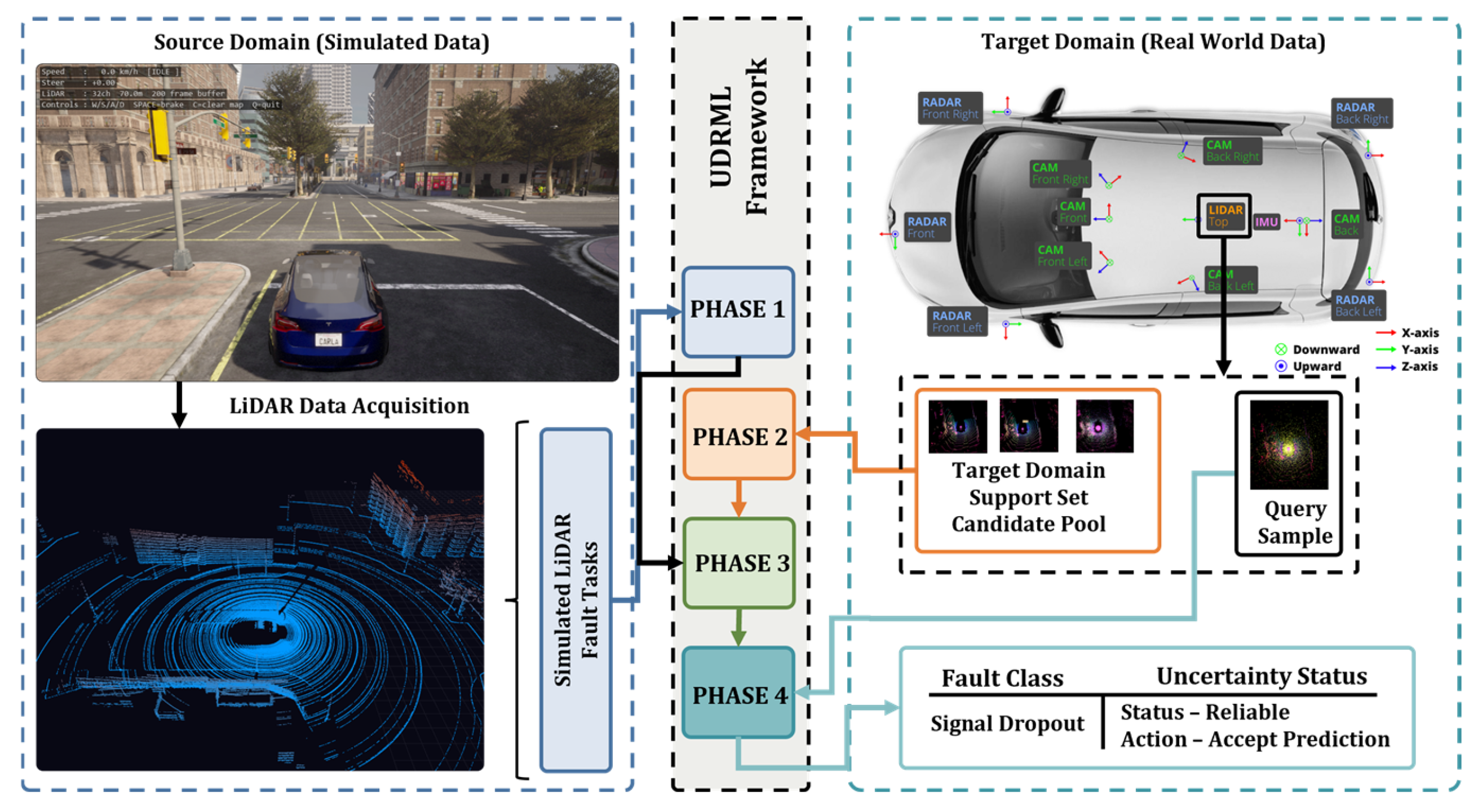
We consider eight LiDAR fault scenarios (including the nominal case) spanning three categories: environmental (rain, snow, fog), sensor-internal (signal dropout, sensor jitter), and scene-interaction (ghosting, occlusion). All samples are processed in bird’s-eye-view (BEV) projections for feature extraction by the CNN backbone of MTDA. Raw LiDAR point clouds are projected into a three-channel BEV image by discretizing 3D space into a 2D grid. Each cell $\left(i,j\right)$ encodes a height map $M_H$ (max $\mathrm{z}$-coordinate), an intensity map $M_I$ (mean reflectivity), and a log-scaled density map $M_D=ln\left(1+N_{ij}\right)$. Channels are normalized to $\left[\mathrm{0,255}\right]$ and stacked as an $84\times 84$ RGB image. Figure 3 summarizes this data flow, linking the LiDAR inputs and BEV representations to the UDRML classification framework.

Figure 3. Overview of data flow in the UDRML framework. Blue, orange, green, and teal identify Phases 1–4: meta-training, active sampling, adaptation, and ensemble inference which are visualized in Figure 1.

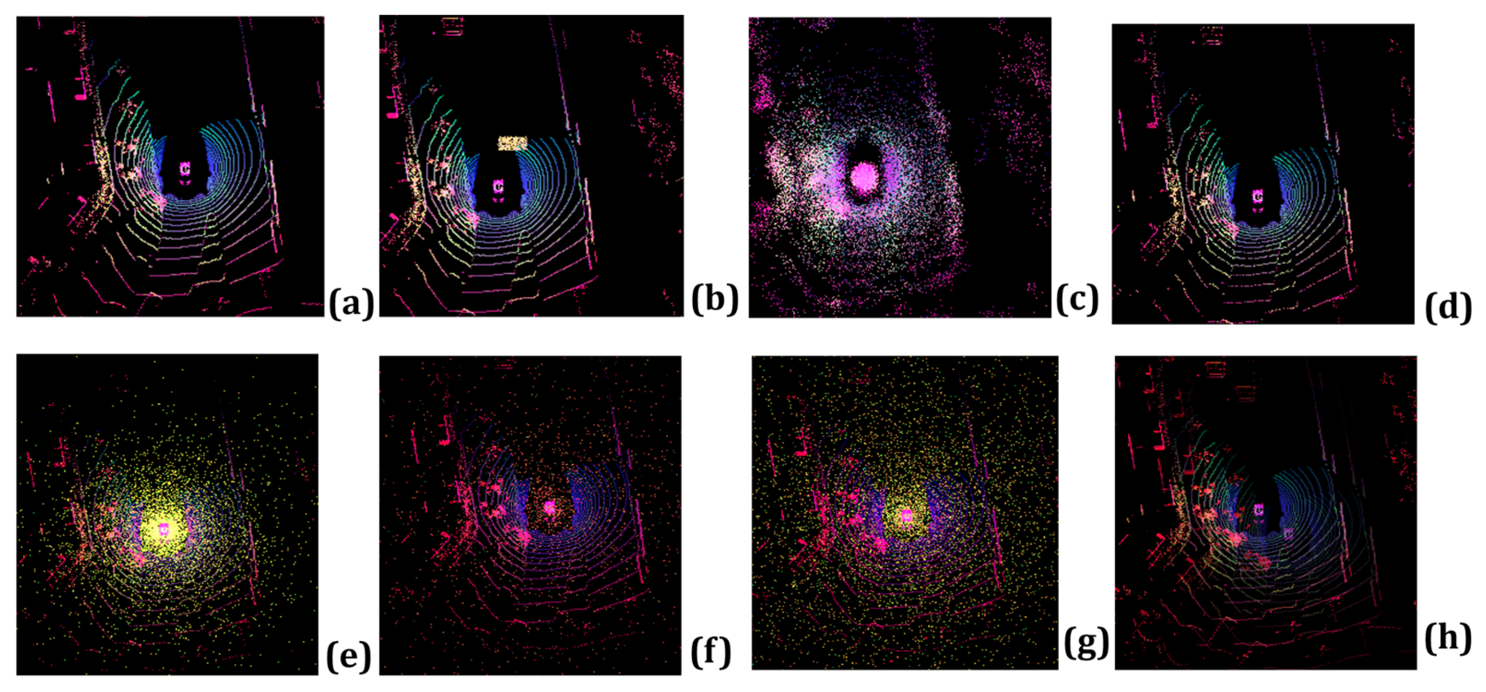
Synthetic LiDAR point clouds for the source domain were generated using NVIDIA Omniverse Isaac Sim (v4.0.0) with USD (v23.11) and MDL for physically based reflections, yielding 600 samples per fault class across three severity levels (per-fault severity ranges and simulation methods are listed in Table S2). The target domain is built on nuScenes [45], collected in Boston, MA, USA, and Singapore using a Velodyne HDL-32E LiDAR sensor, with rain and occlusion extracted directly via metadata filtering and 3D annotation analysis to preserve real sensor degradation. Snow and fog are sourced from the Weather-NuScenes benchmark [46], which applies physically calibrated atmospheric augmentation with point-level labels. Sensor-internal and scene-interaction faults (dropout, jitter, ghosting), which cannot manifest in a functioning sensor dataset, are generated through controlled injection on clean nuScenes scans (structured channel/azimuth removal, Gaussian perturbation at $\sigma =0.03$ m, and duplicate-point insertion at plausible reflection offsets, respectively); the per-fault data origins and acquisition details are in Table S3. Each fault class contains 200 labeled samples, yielding 1600 target-domain samples across eight classes: per class, 100 form the support candidate pool and a disjoint 100 form the evaluation query set (800 support candidates and 800 query samples in total)—a deliberately constrained pool that reflects deployment conditions where extensive real fault data are unavailable. The synthetic source domain comprises samples generated across 12 independent Isaac Sim scenes per fault class; the target domain draws on 25 distinct nuScenes scenes for rain and 18 for occlusion, 30 scenes from the Weather-NuScenes subsets for snow and fog, and 40 clean scenes used for controlled injection. Support sets of K = 5, 10, 20, or 50 samples per class are drawn from the candidate pool. Full per-class counts, scene counts, and origin labels are provided in Supplementary Table S6. A sample visualization of the target-domain dataset (mixed-origin) is given in Figure 4.

Figure 4. Sample image from the target-domain dataset (mixed-origin)—(a) Reference normal BEV projection, (b) Obstacle/occlusion class, (c) Sensor jitter, (d) Signal dropout, € Fog, (f) Rain, (g) Snow, (h) Ghosting.

4.2. Comparative Methods and Backbone

UDRML is compared against nine baselines: four meta-learning methods without uncertainty components—MAML [13], Reptile [47], Matching Networks [48], ProtoNet+ [49]—and five UQ methods—MC Dropout [24] ($\mathrm{T}=20$ passes), SVGD [26] and S²VGD [27] ($\mathrm{n}=10$ particles each), and EMP and ECMP [30] ($M=4$). UDRML uses $\mathrm{M}=4$ ensemble members. A side-by-side overview of the baseline categories, UQ types, and ensemble sizes is provided in Table S4. All MTDA modules share the standard 4-layer convolutional backbone from the original MAML framework so that performance differences reflect the learning strategy rather than the architecture. Each block applies (Conv $3\times 3$, 64) + BN + ReLU + MaxPool $2\times 2$, taking the BEV input from $3\times 84\times 84$ down to $64\times 5\times 5$, flattened to a 1600-dim feature vector and projected to 8 logits via a final linear layer (~113K parameters); the layer-by-layer specification is given in Table S5. The network outputs raw logits; softmax is applied externally for entropy computation and ensemble inference. All models use $G=5$ domain adaptation steps, following [13].

All methods share the following training protocol. Meta-training uses the Adam optimizer (β₁ = 0.9, β₂ = 0.999) with outer learning rate β = 0.001 held constant (no schedule), a meta-batch of N = 4 tasks, and 10,000 meta-training episodes; inner-loop settings are as specified in Table 1. Baseline hyperparameters were tuned by grid search over each method’s primary hyperparameters (learning rate ∈ {10⁻³, 10⁻², 10⁻¹}; dropout/particle/ensemble settings at their published defaults), selecting the configuration with the highest validation accuracy, on a validation split comprising 20% of the target-domain pool, drawn from the support candidate portion so that the evaluation query sets are never used for tuning, and the same split is used to derive the decision gate thresholds τ_high and τ_low (Section 3.3.2). All reported results are averaged over five independent runs with seeds {0, 1, 2, 3, 4}; the seeds governing Latin Hypercube partitioning and the support/query splits are fixed to 0 across all experiments.

5. Results

5.1. Classification Accuracy

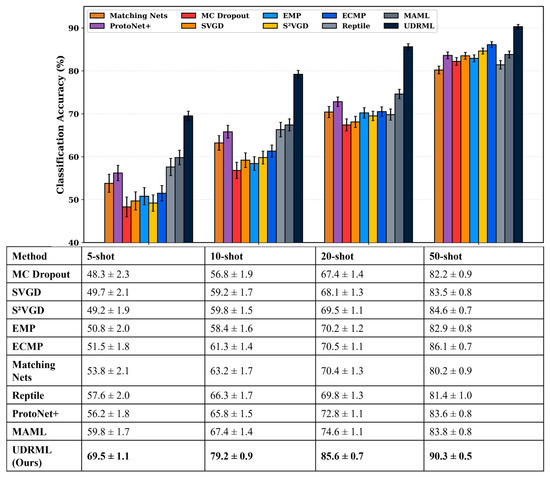
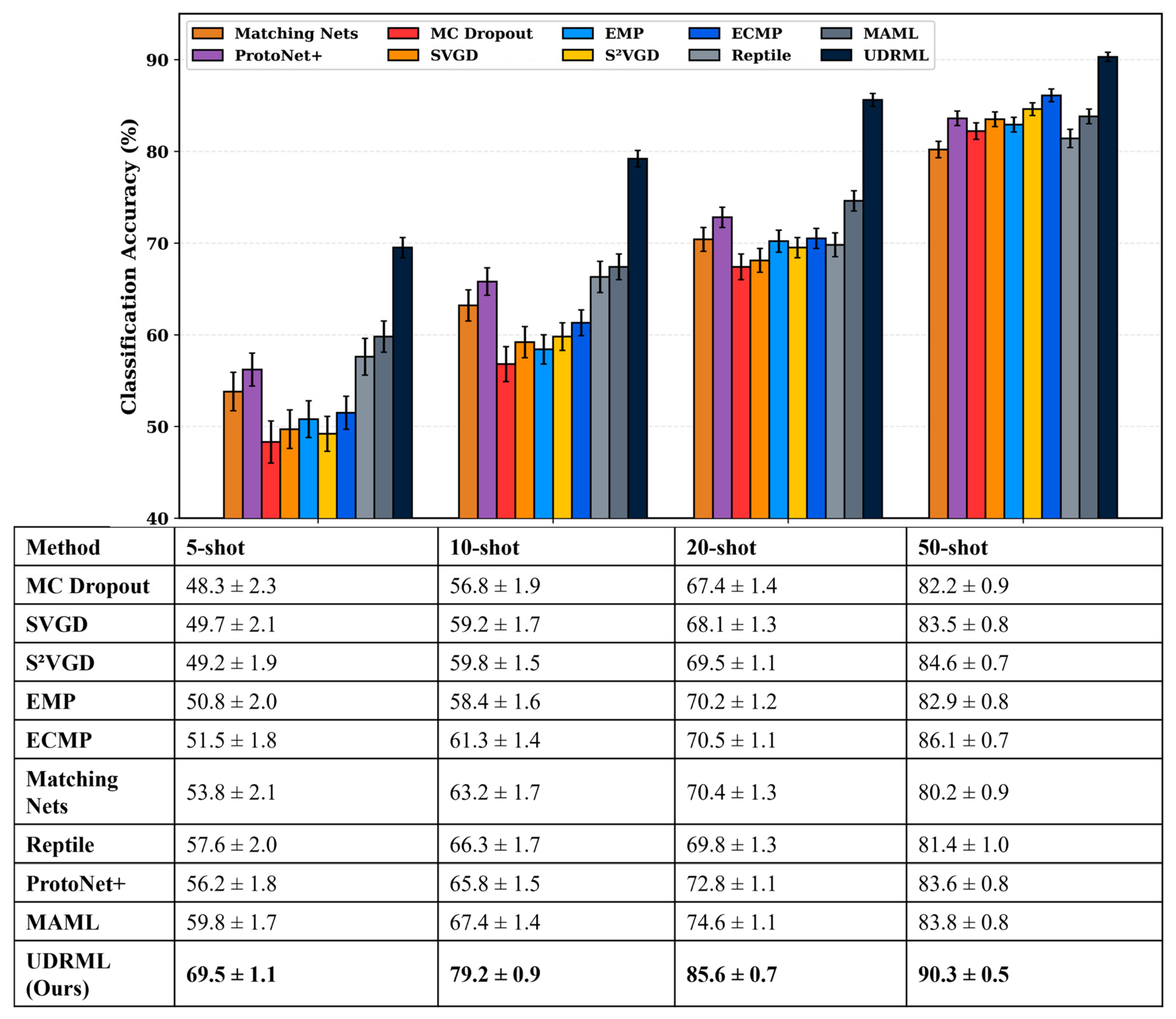
Figure 5 reports classification accuracy across all methods and four shot settings, averaged over five independent runs. UDRML reaches 69.5%, 79.2%, 85.6%, and 90.3% at $\mathrm{K}=5,10,20,50,$ respectively—the highest values among the tested baselines in each setting. Two regimes emerge across the shot spectrum. At low shots (5, 10), meta-learning methods lead the conventionally trained UQ baselines: MAML (59.8%) is 8.3 points above the strongest UQ baseline ECMP (51.5%) at 5-shot, and ProtoNet+ (56.2%) and Reptile (57.6%) similarly outperform all conventionally trained methods, consistent with the expectation that a meta-learned initialization helps when adaptation data are scarce. The ordering partially inverts at 50-shot, where ECMP (86.1%) and S²VGD (84.6%) overtake MAML (83.8%): with 50 support samples, well-calibrated conventional methods become competitive with meta-learning. UDRML’s improvement over MAML peaks at 10-shot (+11.8 points), the regime where meta-learning provides sufficient adaptation capability and entropy-driven sample selection offers the largest marginal benefit. The gap narrows at 50-shot (+4.2 points over ECMP), as expected when increased data reduces the impact of active sampling. Across all settings, UDRML shows the lowest variance ($\pm 0.5$ to $\pm 1.1$) among the methods tested, approximately half the baseline average, consistent with a stabilizing effect of the hyper-ensemble. Because the target classes are balanced, accuracy is an appropriate headline metric; for completeness, macro-F1, macro-precision, macro-recall, and balanced accuracy are reported for all methods in Supplementary Table S7—the method ranking is unchanged under all four metrics (UDRML macro-F1 0.786 vs. 0.662 for the strongest baseline).

Figure 5. Visualization of classification accuracy (%) vs. no. of shots.

5.2. Per-Fault Analysis and Feature Separability

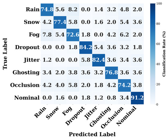
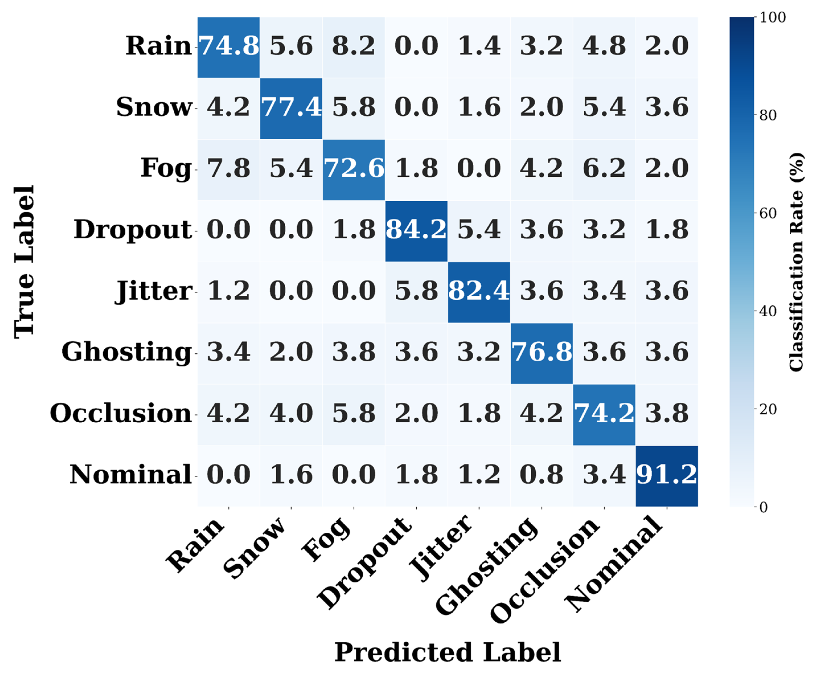
Table 2 disaggregates 10-shot results across the eight classes. Sensor-internal faults (dropout 84.2%, jitter 82.4%) are classified most reliably across methods, followed by environmental (snow 77.4%, rain 74.8%, fog 72.6%) and scene-interaction faults (ghosting 76.8%, occlusion 74.2%). Fog is the hardest fault for every method tested: its dense near-field backscatter alters point cloud geometry in ways no method we evaluated fully overcomes. UDRML’s 72.6% on fog is +14.0 points above MAML, in line with entropy-based sample selection being most useful when fault signatures are obscured by aleatoric noise. The data origin pattern is consistent with the hybrid dataset design: the injected sensor-internal faults (dropout, jitter) are the easiest classes, while the hardest classes (fog, occlusion, rain) all retain real or physically calibrated degradation, suggesting that naturally occurring degradation presents a domain gap synthetic injection does not fully replicate. UDRML’s improvements over MAML are concentrated on these harder classes (fog +14.0, rain +12.4, occlusion +14.0), in line with the uncertainty-aware pipeline contributing the most where the transfer challenge is largest. Aggregated by data origin, UDRML attains 80.1% on naturally occurring faults (rain, occlusion, nominal), 75.0% on physically augmented faults (snow, fog), and 81.1% on injected faults (dropout, jitter, ghosting), versus 68.3%, 62.2%, and 69.9% for MAML; the physically augmented environmental classes are the hardest for every method, and UDRML’s margin is largest there (+12.8 points). The distributional basis of this pattern is quantified by the per-class maximum mean discrepancy (MMD) between synthetic-domain and target-domain feature embeddings: the gap is largest for the environmental classes (fog 0.42, rain 0.38) and smallest for the injected faults (dropout 0.14), and per-class MMD correlates with per-class difficulty, quantifying this domain gap directly.

Table 2. Per-fault classification accuracy (%) at 10-shot.

Fault	Origin	MC Dr.	SVGD	S2VGD	EMP	ECMP	M.Nets	Pnet+	Rept.	MAML	UDRML
Rain	Real	50.6	53.4	54.2	52.6	55.2	57.4	60.2	60.8	62.4	74.8
Snow	Semi-real	54.8	57.2	57.8	56.4	59.6	61.6	64.0	64.6	65.8	77.4
Fog	Semi-real	47.2	49.8	50.4	48.8	52.4	53.8	56.4	57.2	58.6	72.6
Dropout	Injected	63.4	65.8	66.4	64.8	67.8	69.8	72.2	72.4	73.8	84.2
Jitter	Injected	60.8	63.2	63.8	62.2	65.2	67.2	69.8	70.2	71.4	82.4
Ghosting	Injected	53.2	55.6	56.4	54.8	58.4	60.0	62.4	62.8	64.6	76.8
Occlusion	Real	48.4	51.2	51.8	50.4	53.8	55.6	58.2	58.4	60.2	74.2
Nominal	Real	76.0	77.4	77.6	77.2	78.0	80.2	83.2	84.0	82.4	91.2
Mean		56.8	59.2	59.8	58.4	61.3	63.2	65.8	66.3	67.4	79.2

The confusion matrix in Figure 6 localizes these errors. Misclassifications concentrate within the environmental block: fog is most frequently confused with rain (7.8% of fog samples), with a smaller leak into snow (5.4%), while rain in turn leaks mainly into fog (8.2%), consistent with all three faults producing diffuse, spatially distributed density perturbations that the BEV projection renders with similar signatures. A comparable cross-block confusion axis links fog and occlusion (6.2% of fog samples are predicted as occlusion, 5.8% conversely), both of which suppress returns over extended regions of the scene. Dropout and jitter retain the cleanest fault diagonals (84.2% and 82.4%) and direct their largest residual errors to each other (5.4% and 5.8%), consistent with their distinctive point-level signatures (structured absence and geometric perturbation, respectively); ghosting shows no dominant confusion partner, its errors spreading nearly uniformly (all below 4%).

Figure 6. Confusion matrix for UDRML at 10-shot. Rows denote true classes, columns denote predicted classes, and entries show percentages within each true class.

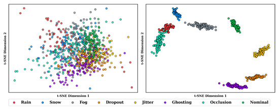
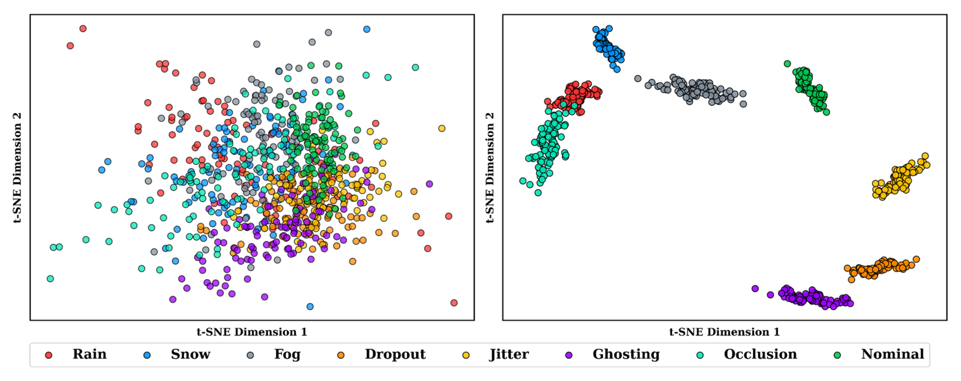
Figure 7 visualizes the 1600-dimensional feature embeddings (extracted before the FC layer) using t-SNE, comparing representations before and after UDRML adaptation at 10-shot. Prior to adaptation, fault classes overlap substantially. After adaptation, class clusters are tighter and more separated, with nominal samples forming the most compact cluster—consistent with its highest classification accuracy (91.2% in Table 2). The environmental classes form neighboring but distinct clusters, with the clearest residual overlap linking rain and occlusion—the two naturally occurring fault classes—while the sensor-internal faults are well separated; as a 2-D projection, t-SNE proximity is qualitative context rather than a direct predictor of specific confusion pairs.

Figure 7. t-SNE visualization of the 1600-dimensional features extracted before the fully connected layer, before (left) and after (right) UDRML adaptation at 10-shot. Colors indicate the eight classes.

5.3. Uncertainty Calibration

Expected Calibration Error (ECE) measures how closely predicted probabilities track empirical correctness. Predictions are grouped into $\mathrm{B}$ confidence bins; for each bin $\mathrm{b}$ we compute the average confidence $\mathit{conf}\left(b\right)$ and the observed accuracy $\mathit{acc}\left(b\right)$, and ECE is the weighted mean of their absolute difference:

$$\mathrm{ECE}={\displaystyle \sum _{b=1}^B}{\displaystyle \frac{n_b}{n}}\hspace{0.17em}|\hspace{0.17em}\mathrm{acc}\left(b\right)-\mathrm{conf}\left(b\right)\hspace{0.17em}|$$

Table 3 reports uncertainty metrics at 10-shot. UDRML reaches an ECE of 0.058, lower than the next best method in this comparison (MAML at 0.138). Among baselines, meta-learning methods (MAML 0.138, Reptile 0.148, ProtoNet+ 0.152, Matching Networks 0.172) achieve lower ECE than the conventionally trained UQ methods (EMP 0.194, ECMP 0.162, SVGD 0.189, S²VGD 0.176), despite lacking explicit uncertainty mechanisms—suggesting meta-learned initialization produces better-calibrated predictions in the few-shot regime evaluated here. On epistemic uncertainty, UDRML (0.17) records a 78% reduction relative to ECMP (0.76), the best-performing UQ baseline in our comparison, consistent with the hyper-ensemble’s structured diversity producing stronger model consensus on this dataset. UDRML is the only method that reports $H_{\mathit{aleatoric}}$ (0.57), enabling the distinction between irreducible data noise and reducible model disagreement that underpins both the active sampling strategy and the reliability score.

Table 3. Uncertainty quantification metrics at 10-shot.

Method	Acc. (%)	${\mathbf{H}}_{\mathbf{total}}$↓	${\mathbf{H}}_{\mathbf{aleat}}$↓	${\mathbf{I}}_{\mathbf{epist}}$↓	ECE ↓	Brier ↓	NLL ↓
MC Dropout	56.8	1.62	-	0.98	0.214	0.398	1.41
SVGD	59.2	1.51	-	0.88	0.189	0.371	1.28
S2VGD	59.8	1.47	-	0.83	0.176	0.362	1.24
EMP	58.4	1.54	-	0.91	0.194	0.379	1.31
ECMP	61.3	1.38	-	0.76	0.162	0.341	1.16
Matching Nets	63.2	-	-	-	0.172	0.352	1.19
ProtoNet+	65.8	-	-	-	0.152	0.334	1.10
Reptile	66.3	-	-	-	0.148	0.329	1.07
MAML	67.4	-	-	-	0.138	0.318	1.02
UDRML (Ours)	79.2	0.74	0.57	0.17	0.058	0.276	0.74

↓ indicates the downward comparison direction used for the listed metrics; - indicates a value not reported in this comparison.

Since ECE measures only the agreement between confidence and accuracy in aggregate, we complement it with two proper scoring rules. The negative log-likelihood (NLL) evaluates the full predictive distribution and penalizes confident errors most heavily, while the Brier score measures the mean squared deviation between the predictive distribution and the one-hot label; unlike ECE, both are minimized only by predictions that are simultaneously accurate and calibrated. As reported in Table 3, UDRML attains an NLL of 0.74 and a Brier score of 0.276, compared with 1.02 and 0.318 for the strongest baseline (MAML), indicating that the improvement in calibration is not an artifact of the binning used by ECE.

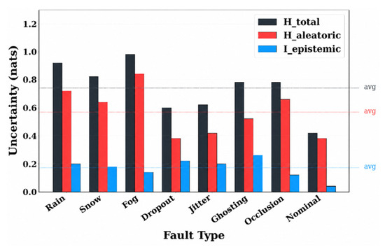
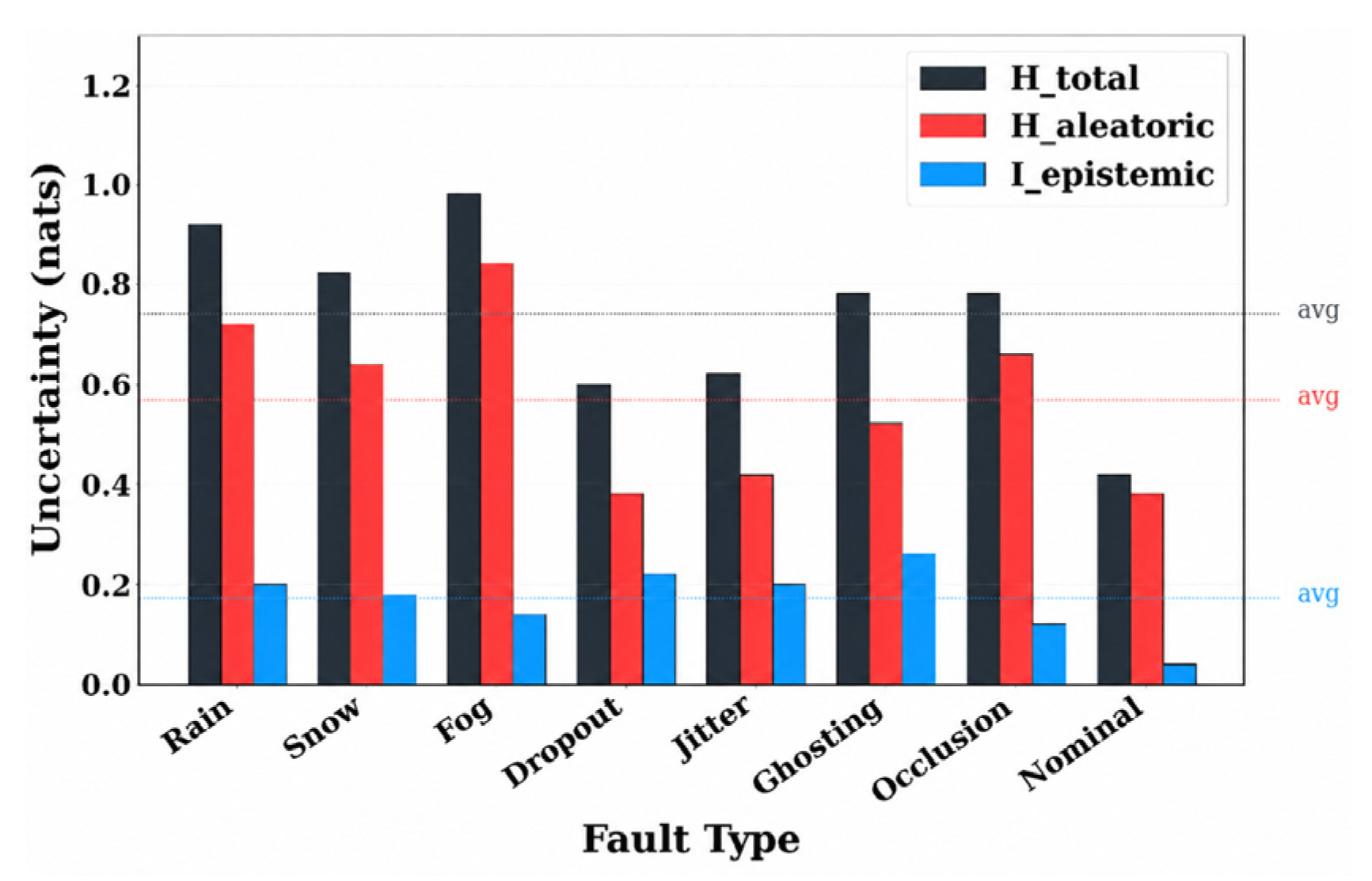
Figure 8 decomposes the three uncertainty components per fault class. Environmental faults exhibit the highest aleatoric uncertainty (fog 0.84, rain 0.72, snow 0.64), in line with their physically noisy signatures. Epistemic uncertainty is highest for ghosting (0.26) and dropout (0.22), where the hyper-ensemble members disagree the most, suggesting these classes occupy regions of the feature space sparsely covered during meta-training. Nominal records the lowest values across all three components ($H_{\mathit{total}}=0.42$, $H_{\mathit{aleatoric}}=0.38$, $I_{\mathit{epistemic}}=0.04$). The per-class decomposition provides diagnostic information beyond aggregate accuracy.

Figure 8. Uncertainty decomposition per fault class (10-shot).

5.4. Active Sampling Behavior

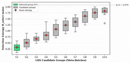
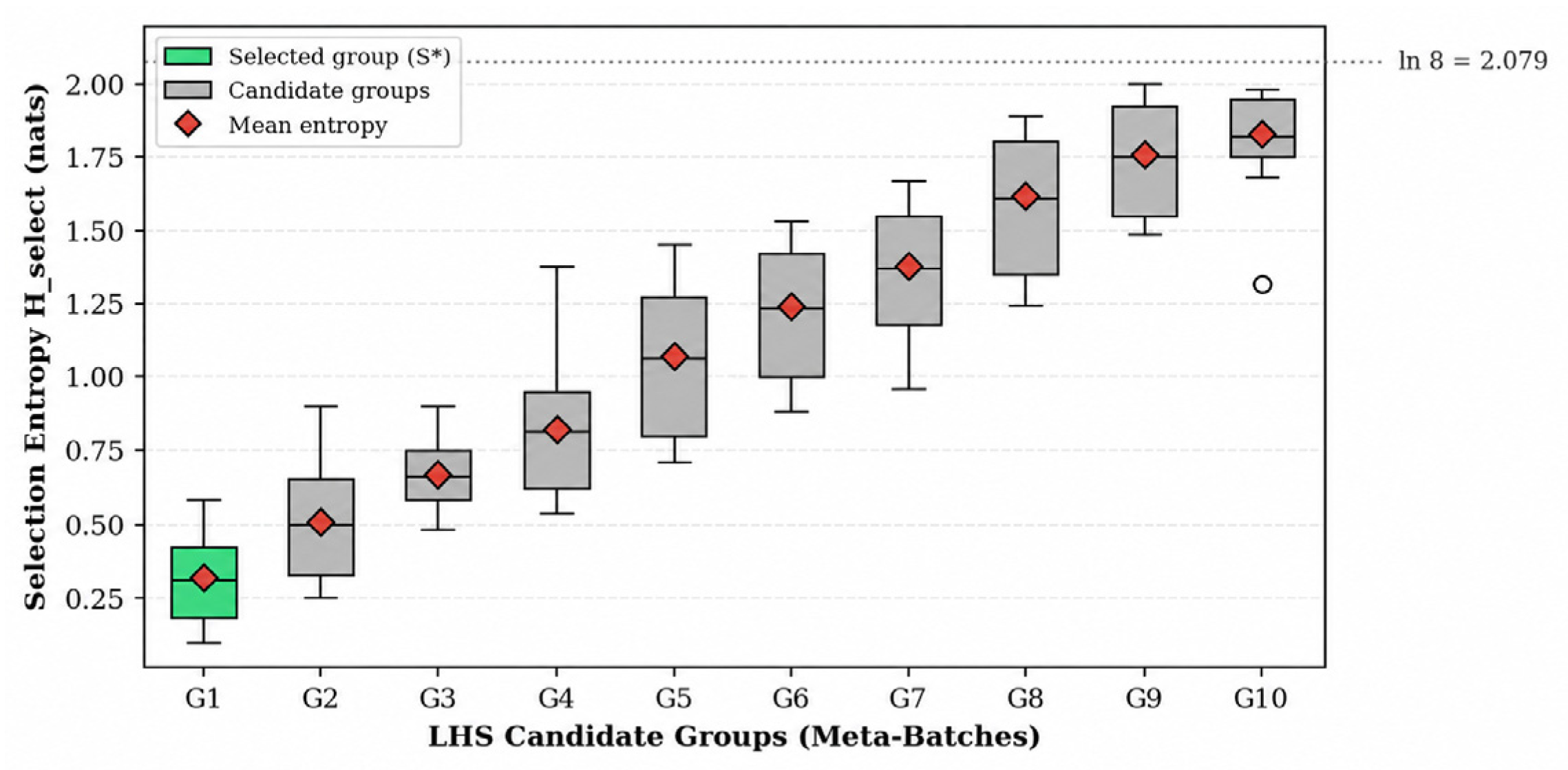
Figure 9 shows the per-group predictive entropy distribution across 10 candidate meta-batches generated via Latin Hypercube Sampling (LHS) under the 10-shot constraint. Selection entropy ($H_{\mathit{select}}$) varies substantially between independently sampled groups, exposing a structural risk of standard random sampling that can ingest non-representative or heavily degraded faulty data—for example, candidate ${\mathrm{G}}_{10}$ produces a spiked average entropy of 1.83 nats. By evaluating predictive uncertainty across the entire LHS pool, UDRML’s active sampling step selects the subset with the lowest mean pre-adaptation predictive entropy (0.32 nats), so that fast-adaptation gradients are anchored on lower-uncertainty support sets—consistent with the +4.8-point accuracy contribution attributed to active sampling in the ablation (Section 5.5).

Figure 9. Per-group entropy distribution during active sampling (10-shot). Green identifies the selected minimum-mean-entropy support set S*; gray identifies the other candidate groups. Red diamonds denote group mean entropy. The dotted horizontal reference line marks the maximum eight-class entropy, ln(8) ≈ 2.079 nats. The superscript * identifies the selected support set.

5.5. Ablation Study

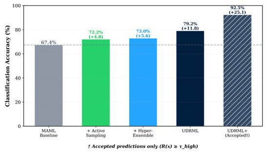
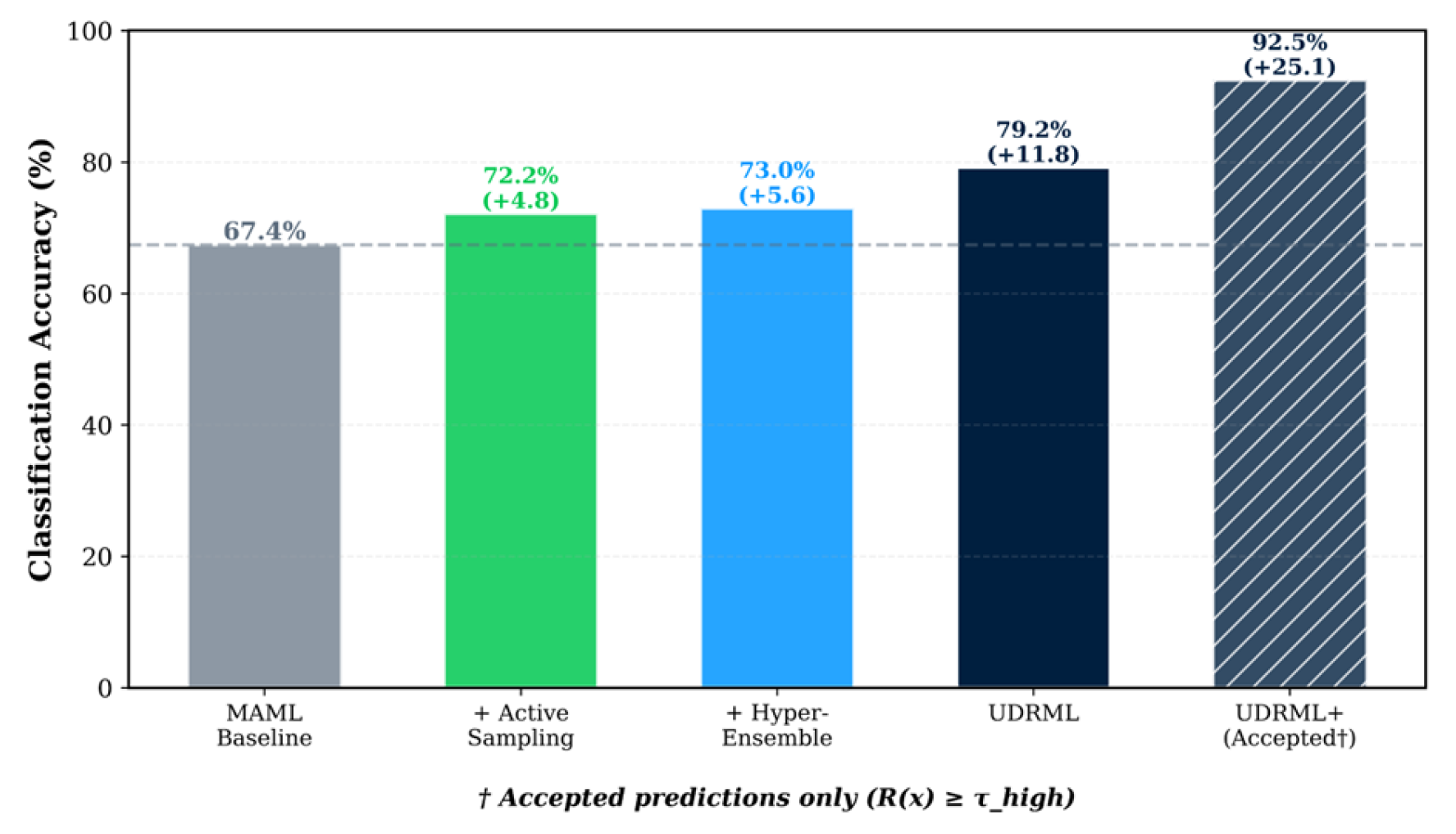
Figure 10 isolates the contribution of each UDRML component at 10-shot. Starting from vanilla MAML (67.4%), adding active sampling alone yields 72.2% (+4.8 points), and adding the hyper-ensemble alone yields 73.0% (+5.6 points). The full UDRML framework reaches 79.2% (+11.8 points), exceeding the sum of individual gains (+10.4 points)—consistent with the two components being complementary rather than redundant. When the reliability-aware decision gate is enabled in UDRML+, classification accuracy is unchanged (79.2%), but accepted prediction accuracy (excluding flagged and rejected samples) rises to 92.5%—a +13.3-point selective improvement obtained by deferring the 23.6% of predictions whose reliability score falls below ${\tau }_{\mathit{high}}$. Of the deferred samples, 15.2% are flagged for secondary verification, and 8.4% are rejected to the fallback path. This is consistent with the gate’s intended behavior: it does not improve the model itself but filters its output, so that lower-confidence predictions are not silently passed downstream.

Figure 10. Component contribution analysis (10-Shot). The dashed horizontal line marks the MAML baseline (67.4%). Values in parentheses are percentage-point gains relative to that baseline. † denotes accuracy evaluated only on accepted predictions with R(x) ≥ τ_high (76.4% coverage), whereas the other bars use all query samples.

Table 4 isolates the contribution of the loss-proportional task weighting of Equation (4b). Replacing it with uniform weights reduces 10-shot accuracy from 79.2% to 77.9%, with the largest per-fault drops on the classes with the greatest sim-to-real discrepancy (fog 2.8 points, rain 1.9 points, occlusion 2.4 points), consistent with the motivation in Section 3.1; accuracy on the well-separated injected faults is essentially unchanged (dropout 0.2 points).

Table 4. Effect of the loss-proportional task weighting (classification accuracy, %, 10-shot).

Variant	Overall	Fog	Rain	Occlusion	Dropout
Uniform weights (wi = 1/N)	77.9	69.8	72.9	71.8	84.0
Loss-proportional (ours)	79.2	72.6	74.8	74.2	84.2

Table 5 evaluates the support set regime across all methods and isolates the selection rule. First, every baseline improves when given the identical curated support set S* (+3.8 points on average), confirming that entropy-driven curation is a method-agnostic contribution; UDRML retains a +7.0-point margin over the strongest curated support baseline, attributable to the hyper-ensemble pipeline. Second, the selection rule controls show that the direction of the entropy criterion matters: selecting the maximum-entropy group (the conventional active learning philosophy) attains 64.8%, below even random sampling, confirming that high-uncertainty exemplars destabilize few-shot adaptation, while minimum-entropy selection over random partitions (71.1%) versus LHS partitions (72.2%) isolates the contribution of coverage-preserving partitioning.

Table 5. 10-shot classification accuracy (%) under random versus curated support sets, with selection rule controls.

Method	Random Support	Curated S*	Δ
MC Dropout	56.8	60.1	+3.3
SVGD	59.2	62.5	+3.3
S2VGD	59.8	63.3	+3.5
EMP	58.4	61.9	+3.5
ECMP	61.3	65.0	+3.7
Matching Nets	63.2	67.1	+3.9
ProtoNet+	65.8	69.6	+3.8
Reptile	66.3	70.4	+4.1
MAML	67.4	72.2	+4.8
UDRML (ours)	-	79.2	-
Selection rule controls (MAML):
Max-entropy LHS group	-	64.8	-
Min-entropy, random partitions (no LHS)	-	71.1	-

- indicates that the corresponding result or matched random-support comparison is not reported in this table; no Δ is calculated for these rows.

Table 6 quantifies the contribution of each diversity axis in the hyper-ensemble. Restricting diversity to a single axis (M = 4 in all configurations) degrades performance: a seed-only ensemble (equivalent to a standard deep ensemble) reaches 76.5%, an inner learning rate-only ensemble 77.6%, and a dropout-only ensemble 76.9%, against 79.2% for the full three-axis configuration. Because the epistemic term of Equation (15) is by definition the inter-member disagreement, the mean I_epist column also quantifies each configuration’s effective diversity: the seed-only ensemble exhibits the least disagreement (0.10), consistent with members converging to similar regions of the loss landscape, while the full configuration attains the best calibration (ECE 0.058, Brier 0.276, NLL 0.74), consistent with hyperparameter diversity capturing uncertainty modes that random initialization alone does not [22]. Ablation configurations use a single repetition due to computational cost; headline results use five runs.

Table 6. Per-axis ablation of hyper-ensemble diversity (10-shot). Each configuration uses M = 4 members varying only the indicated axis; I_epist denotes the mean epistemic uncertainty of Equation (15).

Ensemble Configuration	Acc. (%)	Mean Iepist	ECE	Brier	NLL
Seed-only (deep ensemble)	76.5	0.10	0.081	0.312	0.92
α-only (inner learning rate)	77.6	0.14	0.070	0.298	0.85
Dropout-only	76.9	0.12	0.077	0.305	0.89
Full three-axis (ours)	79.2	0.17	0.058	0.276	0.74

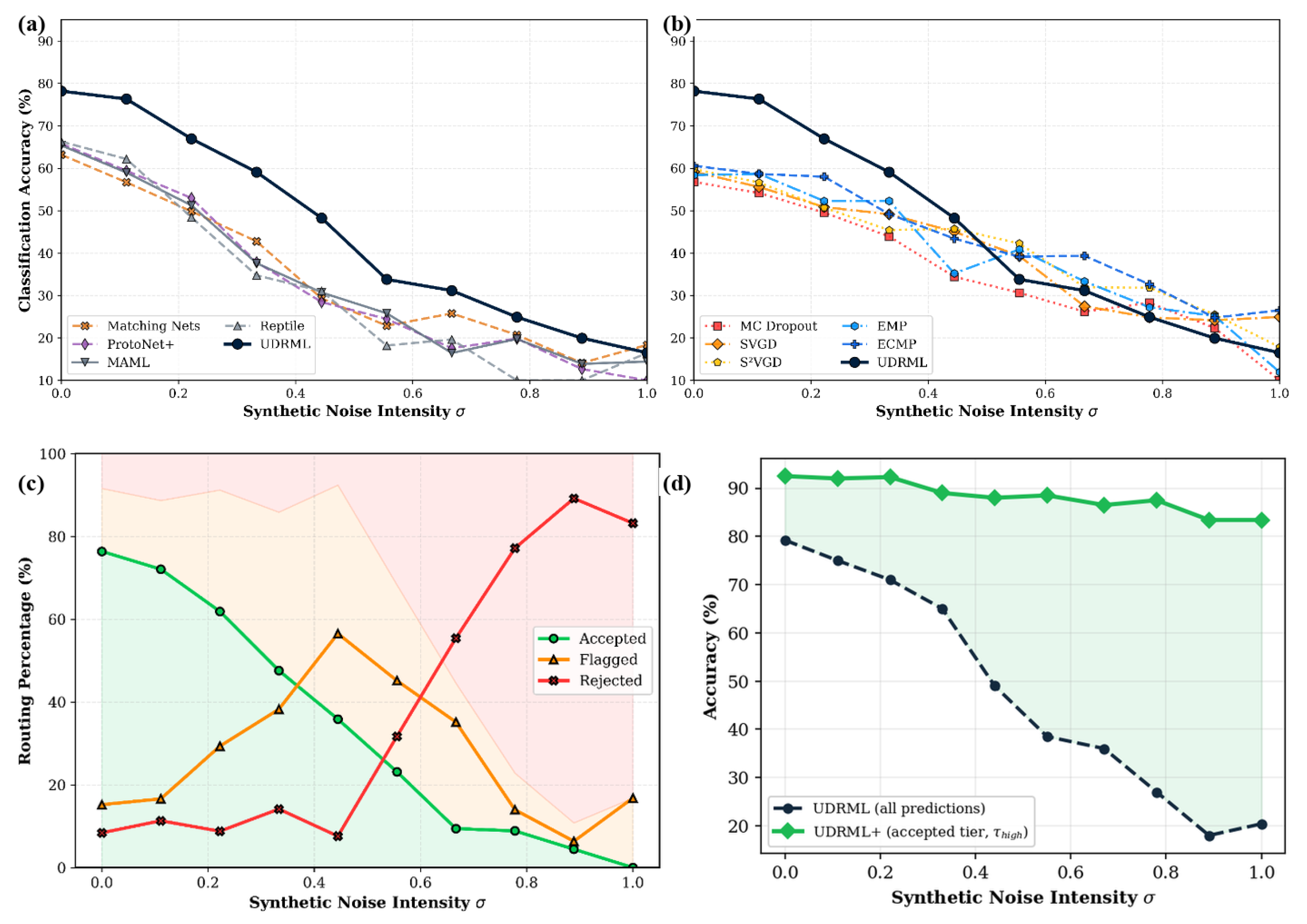
Figure 11a,b evaluates robustness under progressively increasing synthetic noise ($\mathsf{\sigma }\in \left[\mathrm{0,1.0}\right]$). From a 10-shot baseline of 79.2%, UDRML degrades more gradually than the meta-learning baselines and the UQ methods we compared against, retaining relatively strong accuracy under moderate noise ($\mathsf{\sigma }<0.4$). Figure 11c analyses the tri-state routing behavior: under clean conditions, most samples are accepted (76.4%) and few rejected (8.4%), while at $\mathsf{\sigma }=1.0$ the accepted fraction drops to 0.7% and the rejected fraction rises to 83.4%, indicating that the gate progressively routes lower-confidence samples away from automatic prediction as uncertainty rises. Sweeping ${\mathsf{\tau }}_{\mathrm{high}}$ reduces the volume of accepted predictions while increasing their classification precision; setting ${\mathsf{\tau }}_{\mathrm{low}}$ to the chosen point limits rejections to 8.4% of the dataset. Figure 11d evaluates the gate under increasing noise: without gating, UDRML accuracy drops from 79.2% at $\mathsf{\sigma }=0$ to 20.4% at $\mathsf{\sigma }=1.0$, while with the ${\mathsf{\tau }}_{\mathrm{high}}$ acceptance rule, the accepted subset is markedly more stable, decreasing from 92.5% to 83.4%—suggesting that the gate helps preserve the reliability of accepted predictions under increasing distribution shift.

Figure 11. Noise robustness of UDRML and the decision gate (sigma from 0 to 1.0): (a) accuracy degradation versus traditional meta-learners; (b) versus uncertainty quantification baselines; (c) decision gate routing flow (accepted/flagged/rejected fractions); (d) accepted-tier accuracy of UDRML+ versus ungated UDRML. In (c), the green, orange, and red shaded regions represent the accepted, flagged, and rejected fractions, respectively. In (d), the shaded region highlights the difference between accepted-tier and ungated accuracy.

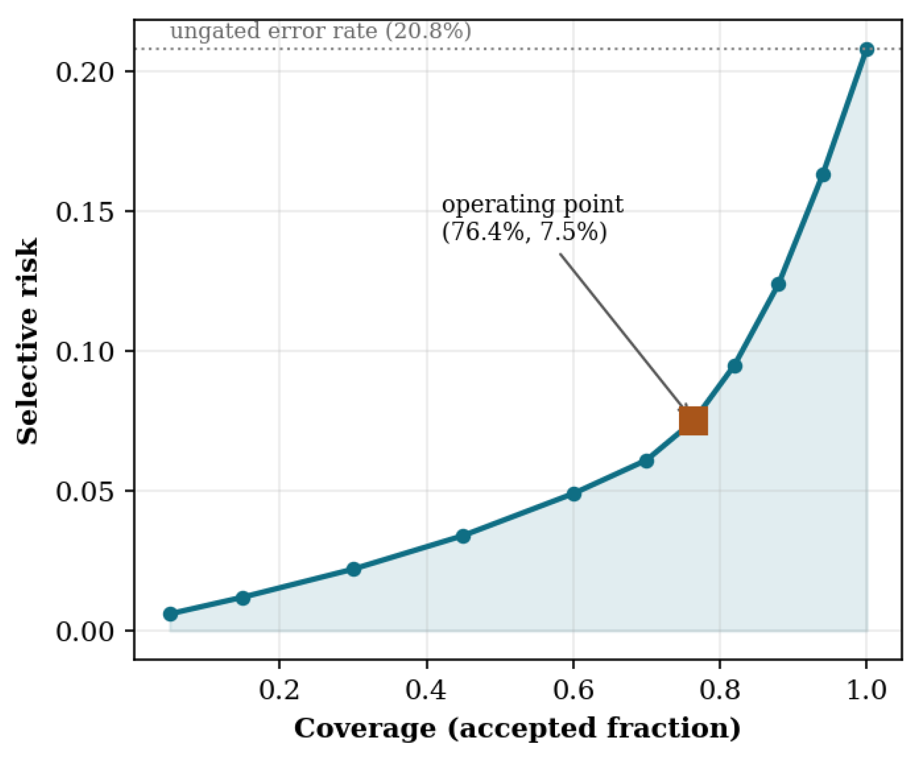
Figure 12 shows risk versus coverage as the acceptance threshold τ_high varies. Coverage is the accepted fraction; risk is the error rate among accepted predictions. The default operating point has 76.4% coverage and 92.5% selective accuracy (AURC = 0.058). Accuracy is lower in the flagged and rejected tiers, at 45.0% and 20.1%, respectively. Gating therefore reduces the error rate on automatically accepted predictions from 20.8% to 7.5%, while directing deferred cases to verification or a fallback.

Figure 12. Risk-coverage curve of the reliability gate under clean conditions, traced by sweeping tau-high (AURC = 0.058), with the operating point (coverage 76.4%, selective risk 7.5%) marked and the ungated error rate shown dotted.

The weights λ₁ and λ₂ control the gate’s relative sensitivity to estimated data noise and model disagreement (Section 3.3.2). Its two thresholds distinguish cases requiring secondary verification from those requiring a fallback. This provides more detailed routing than a single confidence threshold.

5.6. Limitations

Table 7 quantifies the computational overhead. UDRML requires M = 4 independent meta-training runs (12.8 h total versus 3.1 h for a single MAML model) and M forward passes per query: 3.2 ms sequentially, reduced to 1.1 ms when the members are evaluated as a single batched forward pass, lower than the sampling-based uncertainty baselines MC Dropout (T = 20 passes, 15.7 ms) and SVGD (10 particles, 7.9 ms), and negligible against a typical LiDAR frame budget of 50–100 ms at 10–20 Hz; the remaining baselines lie between the single-model and particle-based extremes. Fault monitoring also need not run on the per-frame perception path: fault states evolve over seconds, so the diagnostic layer can execute asynchronously or on every 10-th frame. For deployments with stricter budgets, three parameter-efficient routes are available: shared-backbone ensembles with lightweight diverse heads, BatchEnsemble-style rank-one perturbations within the meta-learning loop [29], and distillation of the ensemble’s mean prediction and uncertainty into a single student model [50].

Table 7. Measured computational cost on the RTX A4000 (10-shot configuration). Latency is the mean over at least 300 queries after warm-up; the batched row evaluates all ensemble members in a single forward pass.

Quantity	MAML	UDRML (M = 4)	MC Dropout (T = 20)	SVGD (n = 10)
Training time, total (h)	3.1 h	12.8 h (4 × 3.2 h)	2.4 h	8.6 h
Adaptation per task (s)	0.4 s	1.7 s	0.4 s	1.1 s
Inference per query, sequential (ms)	0.8 ms	3.2 ms	15.7 ms	7.9 ms
Inference per query, batched members (ms)	-	1.1 ms	-	-
Peak GPU memory, inference (GB)	0.6 GB	0.9 GB	0.6 GB	1.2 GB
Parameters	113 K	452 K	113 K	1.13 M

- indicates that a batched-members latency was not reported for that method; the single-model MAML configuration has no ensemble members to batch.

LHS provides randomized marginal coverage of the candidate pool; selection based on feature-space geometry could further improve diversity. Gate thresholds currently use validation percentiles; learned thresholds could better reflect deployment priorities. Evaluation is limited to LiDAR faults in a synthetically augmented nuScenes setting, so other sensors and diagnostic tasks require validation.

The evaluation covers eight fault classes under a closed-set assumption: the softmax output space is fixed at meta-training time, so a fault type that emerges after deployment cannot be classified without re-meta-training on tasks that include it. Two properties of the framework are relevant to this scenario, though neither is validated here. First, the epistemic component of Equation (15) is by construction largest for inputs unlike the training distribution, so a genuinely novel fault should manifest as high model disagreement and be routed by the decision gate to the flagged or rejected tier rather than silently misclassified, a behavior consistent with the gate’s response to increasing distribution shift in Figure 11d, but not tested against held-out fault categories. Second, scaling to substantially more classes raises the entropy ceiling log C on which both the active sampling criterion and the normalized reliability score depend, so thresholds would require recalibration, and the per-class support requirement grows linearly. Open-set extensions of the classification head and explicit novel fault detection remain future work.

All experiments use BEV projections for compatibility with the convolutional backbone and computational efficiency. These projections compress vertical structure and discard point-level geometry, including details of three-dimensional jitter. Because support selection, ensemble inference, and gating use model logits, other encoders, such as PointNet-style or sparse-voxel models, could be substituted. Whether raw-point processing improves fault classification remains to be tested.

6. Conclusions

UDRML combines entropy-based support selection, ensemble uncertainty decomposition, and reliability gating for few-shot LiDAR fault classification. It achieves 79.2% accuracy at 10-shot and 90.3% at 50-shot, with an 11.8-percentage-point gain over MAML at 10-shot. The gate raises accepted prediction accuracy to 92.5% by deferring uncertain cases, trading coverage for accuracy. This links adaptation with prediction review, allowing limited labeled data to support diagnosis while directing uncertain predictions to verification or fallback.

The findings are limited to eight classes in a mixed-origin LiDAR dataset. BEV projection discards three-dimensional detail, ensembles increase computational cost, and gate thresholds depend on the validation setting. Detection of unseen fault categories and transfer to other sensors remain untested.

Future work should evaluate independent real-world datasets and additional sensing modalities, investigate raw-point or sparse-voxel encoders and open-set fault detection, and reduce computational cost through efficient ensembles or distillation. Thresholds that reflect operational costs could further support deployment.

References

- Qian, H.; Wang, M.; Zhu, M.; Wang, H. A Review of Multi-Sensor Fusion in Autonomous Driving. Sensors 2025, 25, 6033. [Google Scholar] [CrossRef] [Scilit]
- Zhao, J.; Zhao, W.; Deng, B.; Wang, Z.; Zhang, F.; Zheng, W.; Cao, W.; Nan, J.; Lian, Y.; Burke, A.F. Autonomous driving system: A comprehensive survey. Expert Syst. Appl. 2024, 242, 122836. [Google Scholar] [CrossRef] [Scilit]
- Badue, C.; Guidolini, R.; Carneiro, R.V.; Azevedo, P.; Cardoso, V.B.; Forechi, A.; Jesus, L.; Berriel, R.; Paixão, T.M.; Mutz, F.; et al. Self-driving cars: A survey. Expert Syst. Appl. 2021, 165, 113816. [Google Scholar] [CrossRef] [Scilit]
- Matos, F.; Bernardino, J.; Durães, J.; Cunha, J. A Survey on Sensor Failures in Autonomous Vehicles: Challenges and Solutions. Sensors 2024, 24, 5108. [Google Scholar] [CrossRef] [Scilit]
- Xia, Z.-X.; Fadadu, S.; Shi, Y.; Foucard, L. Robust Long-Range Perception Against Sensor Misalignment in Autonomous Vehicles. In 2025 IEEE/CVF Winter Conference on Applications of Computer Vision (WACV); IEEE: Piscataway, NJ, USA, 2025; pp. 5761–5770. [Google Scholar] [CrossRef] [Scilit]
- Kong, X.; Cai, B.; Yu, Y.; Yang, J.; Wang, B.; Liu, Z.; Shao, X.; Yang, C. Intelligent diagnosis method for early faults of electric-hydraulic control system based on residual analysis. Reliab. Eng. Syst. Saf. 2025, 261, 111142. [Google Scholar] [CrossRef] [Scilit]
- Kong, X.; Cai, B.; Liu, Y.; Zhu, H.; Liu, Y.; Shao, H.; Yang, C.; Li, H.; Mo, T. Optimal sensor placement methodology of hydraulic control system for fault diagnosis. Mech. Syst. Signal Process. 2022, 174, 109069. [Google Scholar] [CrossRef] [Scilit]
- Fan, C.; Zhang, Y.; Ma, H.; Ma, Z.; Yin, X.; Zhang, X.; Zhao, S. A novel imbalance fault diagnosis method based on data augmentation and hybrid deep learning models. Struct. Health Monit. 2024, 25, 281–302. [Google Scholar] [CrossRef] [Scilit]
- Zhang, Z.; Shao, M.; Wang, L.; Shao, S.; Ma, C. A Novel Domain Adaptation-Based Intelligent Fault Diagnosis Model to Handle Sample Class Imbalanced Problem. Sensors 2021, 21, 3382. [Google Scholar] [CrossRef] [Scilit]
- Abboush, M.; Knieke, C.; Rausch, A. Representative Real-Time Dataset Generation Based on Automated Fault Injection and HIL Simulation for ML-Assisted Validation of Automotive Software Systems. Electronics 2024, 13, 437. [Google Scholar] [CrossRef] [Scilit]
- Xie, T.; Huang, X.; Choi, S.-K. Intelligent Mechanical Fault Diagnosis Using Multisensor Fusion and Convolution Neural Network. IEEE Trans. Ind. Inform. 2022, 18, 3213–3223. [Google Scholar] [CrossRef] [Scilit]
- Zhang, S.; Ye, F.; Wang, B.; Habetler, T. Few-Shot Bearing Fault Diagnosis Based on Model-Agnostic Meta-Learning. IEEE Trans. Ind. Appl. 2021, 57, 4754–4764. [Google Scholar] [CrossRef] [Scilit]
- Finn, C.; Abbeel, P.; Levine, S. Model-Agnostic Meta-Learning for Fast Adaptation of Deep Networks. In Proceedings of the 34th International Conference on Machine Learning (ICML 2017), Sydney, Australia, 6–11 August 2017. [Google Scholar]
- Yang, T.; Tang, T.; Wang, J.; Qiu, C.; Chen, M. A novel cross-domain fault diagnosis method based on model agnostic meta-learning. Measurement 2022, 199, 111564. [Google Scholar] [CrossRef] [Scilit]
- Xie, T.; Huang, X.; Choi, S.-K. Metric-Based Meta-Learning for Cross-Domain Few-Shot Identification of Welding Defect. J. Comput. Inf. Sci. Eng. 2023, 23, 030902. [Google Scholar] [CrossRef] [Scilit]
- Antoniou, A.; Edwards, H.; Storkey, A. How to train your MAML. In Proceedings of the Seventh International Conference on Learning Representations (ICLR 2019), New Orleans, LA, USA, 6–9 September 2019. [Google Scholar]
- Liang, K.J.; Rangrej, S.B.; Petrovic, V.; Hassner, T. Few-shot Learning with Noisy Labels. In 2022 IEEE/CVF Conference on Computer Vision and Pattern Recognition (CVPR); IEEE: Piscataway, NJ, USA, 2022; pp. 9079–9088. [Google Scholar] [CrossRef] [Scilit]
- Prudencio, R.B.C.; Ludermir, T.B. Active Selection of Training Examples for Meta-Learning. In 7th International Conference on Hybrid Intelligent Systems (HIS 2007); IEEE: Piscataway, NJ, USA, 2007; pp. 126–131. [Google Scholar] [CrossRef] [Scilit]
- Li, K.; Wang, L.; Gao, X.; Zhang, L. Transformer-enhanced meta-learning for few-shot fault diagnosis of electric submersible pump. Expert Syst. Appl. 2025, 284, 127851. [Google Scholar] [CrossRef] [Scilit]
- He, Y.; Shen, W. MSRCN: A cross-machine diagnosis method for the CNC spindle motors with compound faults. Expert Syst. Appl. 2023, 233, 120957. [Google Scholar] [CrossRef] [Scilit]
- Mallick, M.; Shim, Y.-D.; Won, H.-I.; Choi, S.-K. Ensemble-Based Model-Agnostic Meta-Learning with Operational Grouping for Intelligent Sensory Systems. Sensors 2025, 25, 1745. [Google Scholar] [CrossRef] [Scilit]
- Wenzel, F.; Snoek, J.; Tran, D.; Jenatton, R. Hyperparameter ensembles for robustness and uncertainty quantification. In Proceedings of the 34th International Conference on Neural Information Processing Systems (NeurIPS 2020), Vancouver, BC, Canada; Curran Associates Inc.: New York, NY, USA; p. 546.
- Blundell, C.; Cornebise, J.; Kavukcuoglu, K.; Wierstra, D. Weight uncertainty in neural networks. In Proceedings of the ICML’15: Proceedings of the 32nd International Conference on Machine Learning; Association for Computing Machinery: New York, NY, USA, 2015; Volume 37, pp. 1613–1622. [Google Scholar]
- Gal, Y.; Ghahramani, Z. Dropout as a Bayesian Approximation: Representing Model Uncertainty in Deep Learning. In Proceedings of the 33rd International Conference on Machine Learning; Balcan, M.F., Weinberger, K.Q., Eds.; PMLR: New York, NY, USA, 2016; Volume 48, pp. 1050–1059. [Google Scholar]
- Kingma, D.P.; Welling, M. Auto-Encoding Variational Bayes. In Proceedings of the 2nd International Conference on Learning Representations, ICLR 2014 Conference Track Proceedings, Banff, AB, Canada, 14–16 April 2014. Bengio, Y., LeCun, Y., Eds. [Google Scholar]
- Liu, Q.; Wang, D. Stein Variational Gradient Descent: A General Purpose Bayesian Inference Algorithm. In Advances in Neural Information Processing Systems; Lee, D., Sugiyama, M., Luxburg, U., Guyon, I., Garnett, R., Eds.; Curran Associates, Inc.: Red Hook, NY, USA, 2016. [Google Scholar]
- Zhang, R.; Li, C.; Chen, C.; Carin, L. Learning Structural Weight Uncertainty for Sequential Decision-Making. arXiv 2018, arXiv:1801.00085. [Google Scholar] [CrossRef] [Scilit]
- Lakshminarayanan, B.; Pritzel, A.; Blundell, C. Simple and scalable predictive uncertainty estimation using deep ensembles. In Proceedings of the 31st International Conference on Neural Information Processing Systems, NIPS’17; Curran Associates, Inc.: Red Hook, NY, USA, 2017; pp. 6405–6416. [Google Scholar]
- Wen, Y.; Tran, D.; Ba, J. BatchEnsemble: An Alternative Approach to Efficient Ensemble and Lifelong Learning. arXiv 2020, arXiv:2002.06715. [Google Scholar]
- Chang, O.; Yao, Y.; Williams-King, D.; Lipson, H. Ensemble Model Patching: A Parameter-Efficient Variational Bayesian Neural Network. arXiv 2019, arXiv:1905.09453. [Google Scholar] [CrossRef] [Scilit]
- Yoon, J.; Kim, T.; Dia, O.; Kim, S.; Bengio, Y.; Ahn, S. Bayesian model-agnostic meta-learning. In Advances in Neural Information Processing Systems 31 (NeurIPS 2018); Curran Associates, Inc.: Red Hook, NY, USA, 2018. [Google Scholar]
- Finn, C.; Xu, K.; Levine, S. Probabilistic model-agnostic meta-learning. In Advances in Neural Information Processing Systems 31 (NeurIPS 2018); Curran Associates, Inc.: Red Hook, NY, USA, 2018. [Google Scholar]
- Lian, Z.; Li, S.; Huang, Q.; Huang, Z.; Liu, H.; Qiu, J.; Yang, P.; Tao, L. UBMF: Uncertainty-aware Bayesian meta-learning framework for fault diagnosis with imbalanced industrial data. arXiv 2025, arXiv:2503.11774. [Google Scholar]
- Liu, Z.; Peng, Z. Few-shot bearing fault diagnosis by semi-supervised meta-learning with graph convolutional neural network under variable working conditions. Measurement 2025, 240, 115402. [Google Scholar] [CrossRef] [Scilit]
- Ho, S.; Liu, M.; Gao, S.; Gao, L. Learning to learn for few-shot continual active learning. Artif. Intell. Rev. 2024, 57, 280. [Google Scholar] [CrossRef] [Scilit]
- Sensoy, M.; Kaplan, L.; Kandemir, M. Evidential deep learning to quantify classification uncertainty. In Proceedings of the 32nd International Conference on Neural Information Processing Systems, NIPS’18; Curran Associates, Inc.: Red Hook, NY, USA, 2018; pp. 3183–3193. [Google Scholar]
- Van Amersfoort, J.; Smith, L.; Teh, Y.W.; Gal, Y. Uncertainty estimation using a single deep deterministic neural network. In Proceedings of the 37th International Conference on Machine Learning, ICML’20; Curran Associates, Inc.: Red Hook, NY, USA, 2020. [Google Scholar]
- Damianou, A.; Lawrence, N.D. Deep Gaussian Processes. In Proceedings of the Sixteenth International Conference on Artificial Intelligence and Statistics; Proceedings of Machine Learning Research Series; Carvalho, C.M., Ravikumar, P., Eds.; PMLR: Scottsdale, AZ, USA, 2013; Volume 31, pp. 207–215. [Google Scholar]
- Wang, J.; Qiang, W.; Su, X.; Zheng, C.; Sun, F.; Xiong, H. Towards task sampler learning for meta-learning. Int. J. Comput. Vis. 2024, 132, 5534–5564. [Google Scholar] [CrossRef] [Scilit]
- Lin, T.-Y.; Goyal, P.; Girshick, R.; He, K.; Dollar, P. Focal loss for dense object detection. In Proceedings of the IEEE International Conference on Computer Vision (ICCV), Venice, Italy, 22–29 October 2017; pp. 2980–2988. [Google Scholar]
- Hullermeier, E.; Waegeman, W. Aleatoric and epistemic uncertainty in machine learning: An introduction to concepts and methods. Mach. Learn. 2021, 110, 457–506. [Google Scholar] [CrossRef] [Scilit]
- Kendall, A.; Gal, Y. What uncertainties do we need in Bayesian deep learning for computer vision? In Proceedings of the 31st International Conference on Neural Information Processing Systems, (NeurIPS), Long Beach, CA USA, 4–9 December 2017. [Google Scholar]
- Depeweg, S.; Hernandez-Lobato, J.M.; Doshi-Velez, F.; Udluft, S. Decomposition of uncertainty in Bayesian deep learning for efficient and risk-sensitive learning. In Proceedings of the 35th International Conference on Machine Learning, Stockholm, Sweden, 10–15 July 2018; pp. 1184–1193. [Google Scholar]
- Wimmer, L.; Sale, Y.; Hofman, P.; Bischl, B.; Hullermeier, E. Quantifying aleatoric and epistemic uncertainty in machine learning: Are conditional entropy and mutual information appropriate measures? In Proceedings of the Conference Uncertainty in Artificial Intelligence (UAI), Pittsburgh, PA, USA, 31 July–4 August 2023; pp. 2282–2292. [Google Scholar]
- Caesar, H. NuScenes: A Multimodal Dataset for Autonomous Driving. In Proceedings of the IEEE/CVF Conference on Computer Vision and Pattern Recognition, Seattle, WA, USA, 13–19 June 2020. [Google Scholar]
- Teufel, S.; Volk, G.; Von Bernuth, A.; Bringmann, O. Simulating Realistic Rain, Snow, and Fog Variations For Comprehensive Performance Characterization of LiDAR Perception. In 2022 IEEE 95th Vehicular Technology Conference: (VTC2022-Spring); IEEE: Piscataway, NJ, USA, 2022; pp. 1–7. [Google Scholar] [CrossRef] [Scilit]
- Nichol, A.; Achiam, J.; Schulman, J. On First-Order Meta-Learning Algorithms. arXiv 2018, arXiv:1803.02999. [Google Scholar]
- Vinyals, O.; Blundell, C.; Lillicrap, T.; Kavukcuoglu, K.; Wierstra, D. Matching Networks for One Shot Learning. In Advances in Neural Information Processing Systems; Lee, D., Sugiyama, M., Luxburg, U., Guyon, I., Garnett, R., Eds.; Curran Associates, Inc.: Red Hook, NY, USA, 2016. [Google Scholar]
- Snell, J.; Swersky, K.; Zemel, R. Prototypical networks for few-shot learning. In Proceedings of the 31st International Conference on Neural Information Processing Systems, NIPS’17; Curran Associates, Inc.: Red Hook, NY, USA, 2017; pp. 4080–4090. [Google Scholar]
- Malinin, A.; Mlodozeniec, B.; Gales, M. Ensemble distribution distillation. In Proceedings of the 8th International Conference on Learning Representations, Virtual, 26 April–1 May 2020. [Google Scholar]
Disclaimer/Publisher’s Note: The statements, opinions and data contained in all publications are solely those of the individual author(s) and contributor(s) and not of MDPI and/or the editor(s). MDPI and/or the editor(s) disclaim responsibility for any injury to people or property resulting from any ideas, methods, instructions or products referred to in the content. |
© 2026 by the authors. Licensee MDPI, Basel, Switzerland. This article is an open access article distributed under the terms and conditions of the Creative Commons Attribution (CC BY) license.