Residual Vibration Suppression in Flexible Systems Using a Tuned Four-Segment Acceleration Profile

Abstract

This study presents a method for tuning input motion to suppress residual vibrations in a flexible link manipulator, with particular relevance to mechatronic positioning systems. The approach is based on a four-segment acceleration profile that combines ramp, cycloid, and ramped-versine trajectories, enabling effective vibration reduction over a wide range of travel times. Unlike the conventional continuous reference profiles considered in this study, the proposed method does not require the total motion duration to be an integer or half-integer multiple of the system’s natural period to suppress residual vibration. The motion consists of acceleration and deceleration phases, each divided into two subsections to ensure smooth transitions. The formulation is developed analytically for both undamped and underdamped systems and is validated through numerical simulations and experiments on a servo-driven mechatronic setup equipped with inertial measurement units. For the cases considered in the quantitative comparison, the proposed method reduced the dominant first-mode residual-vibration amplitude by approximately 97–100% in the simulations and 92–98% in the experiments relative to the corresponding untuned commands. Performance is evaluated using the percent residual vibration (PRV) metric, with comparisons to commonly used motion profiles, including trapezoidal, trigonometric, and cycloidal trajectories. The results indicate that substantial vibration reduction is achieved across different travel times, including cases where the motion duration is shorter than one natural period. Overall, the proposed method offers a practical and flexible alternative to conventional motion tuning techniques and is well suited for high-speed, precision-sensitive applications such as robotic manipulators and automated manufacturing systems.

1. Introduction

Systems built with lightweight, high-speed, and flexible components are common in modern robotics and automation. These characteristics bring clear benefits—lower inertia and higher precision—but they also introduce a persistent challenge. Structural flexibility often leads to residual vibrations, which can be difficult to eliminate once excited. In industrial environments, where positioning accuracy and cycle time directly affect productivity, these vibrations are more than a minor inconvenience. They can degrade performance, reduce accuracy, and, over time, contribute to increased wear and a shorter service life of mechanical components. For this reason, controlling vibration in flexible systems is not merely an academic concern; it is a practical requirement in many real engineering applications.

Traditional approaches to vibration reduction generally fall into two broad categories: feedback and feedforward methods. Feedback control relies on real-time sensor measurements to detect and suppress vibrations as they occur. While this strategy can be effective, it often increases system complexity and cost, since additional sensors, actuators, and control hardware are typically required. Feedforward approaches take a different path. Instead of reacting to vibrations, they aim to prevent them by shaping the reference input so that the system’s resonant modes are not significantly excited. In many cases, this makes feedforward methods easier to implement in practice, and they avoid some of the stability concerns that can arise in closed-loop control systems.

A wide variety of motion profile design methods have been developed to reduce residual vibrations. Many of these approaches can be quite effective, but a large number of them rely on selecting the total motion duration in relation to specific multiples of the system’s natural period in order to achieve complete vibration suppression [1,2]. In practice, this requirement can be restrictive. In many real applications, the cycle time is fixed in advance or constrained by process demands, leaving little freedom to adjust the motion duration. This becomes particularly problematic in high-speed positioning systems, where extending the motion time simply to meet vibration suppression conditions is often not acceptable, since it directly lowers productivity and overall throughput [3].

The main contributions of this study can be summarized as follows:

(1)

A four-segment acceleration profile combining ramp, cycloidal, and ramped-versine components is formulated. Since acceleration acts directly as the excitation input in the modal equation, the component amplitudes are determined analytically at the acceleration level to satisfy the zero-residual-vibration condition of the dominant first mode. In this way, vibration suppression is incorporated directly into the prescribed motion.

(2)

Unlike the conventional continuous motion profiles examined in this study, whose zero-residual-vibration conditions occur at particular motion durations related to the natural period, the proposed formulation does not require the total travel time to satisfy a prescribed integer or half-integer relationship with the natural period. This provides greater flexibility in selecting the motion duration.

(3)

The analytical formulation is developed for both undamped and underdamped flexible systems, allowing the effect of damping to be incorporated directly into the motion-profile design.

(4)

The method is evaluated through numerical simulations and experiments on flexible beams driven by a servo motor and instrumented with inertial measurement units. The results demonstrate substantial suppression of the dominant first-mode residual vibration, including for motion durations shorter than one natural period. Comparisons with trapezoidal, trigonometric, and conventional S-curve motion profiles further demonstrate the effectiveness of the proposed approach over the investigated motion-time range. These characteristics make the proposed approach particularly relevant to motion-planning problems in flexible robotic manipulators and automated manufacturing systems, where rapid motion and residual-vibration suppression are important considerations.

The rest of the paper is organized as follows. Section 2 provides a brief review of the relevant literature. Section 3 introduces the mathematical model of the system. In Section 4, the proposed motion design and tuning methodology is presented in detail. Section 5 describes the experimental setup and the data acquisition process. The simulation and experimental results are then presented and discussed in Section 6. Section 7 presents the parameter-sensitivity analysis and comparison with ZV input shaping. Finally, Section 8 concludes the paper.

2. Literature Review

A considerable number of methods have been reported in the literature for suppressing residual vibrations in flexible mechanical systems. In general, these approaches can be grouped into several categories, including feedforward control techniques, filtering-based methods, and motion profile design strategies that rely on prescribed velocity or acceleration trajectories. Although the specific implementations differ, they all share a common goal: to limit the excitation of the system’s natural modes while keeping motion duration and tracking performance within acceptable bounds. The most relevant studies from each of these groups are briefly reviewed in this section.

A variety of feedforward control strategies have been explored in the literature, yet suppressing vibration in flexible manipulators remains a challenging task. Mohamed and Tokhi [4], for example, compared several techniques—including input shaping, low-pass filtering, and band-stop filtering—evaluating their effectiveness in reducing vibration levels as well as their impact on response time, robustness, and computational complexity. Other researchers have approached the problem from different angles. Cuccio et al. [5] investigated preshaped input laws with a limited number of acceleration steps to reduce residual vibrations during point-to-point motion in elastic systems. Aspinwall [6] introduced a shaping input function based on the harmonics of a sine series to generate torque trajectories. Meckl and Seering [7], focusing on energy minimization, tuned ramped sinusoidal and versine functions to shape input forces. Despite their effectiveness, many of these methods depend on accurate knowledge of the system’s natural frequency, which can be difficult to obtain in practice [8]. In another study, Alnefaie et al. [9] demonstrated that residual vibrations in rotating flexible beams could be reduced by selecting a suitable rise time relative to the beam’s vibration period when using a triangular velocity profile.

Shin and Brennan [10] investigated acceleration shaping methods for controlling residual vibrations in translating and rotating Euler–Bernoulli cantilever beams. Their results showed performance comparable to that achieved with input shaping techniques. However, as in the work of Alnefaie et al. [9], the effectiveness of these methods depends strongly on selecting motion durations with considerable care. In a different line of research, Önsay and Akay [11] proposed multi-switch bang–bang control functions to achieve time-optimal motion. While this approach can produce fast responses, it also relies on accurately determining the switching times, which in turn requires a reliable dynamic model of the system.

Another commonly used approach for generating command signals is to filter the desired trajectory using finite impulse response (FIR) filters, after which convolution with impulse sequences is applied to obtain the reference commands [12,13,14]. This method can be effective, but its performance is often sensitive to uncertainties in system parameters, which can be difficult to account for in practice. To address this issue, Yavuz et al. [15] and Alıcı et al. [16] proposed a robust motion design technique that maintains insensitivity to parameter variations while avoiding additional time delays, offering a practical alternative in situations where precise system identification is not feasible.

A wide range of effective motion profiles—often referred to as S-curve profiles—have been proposed in robotics and manufacturing to achieve fast and precise positioning while limiting residual vibration. Meckl and Arestides [17], for instance, employed well-known S-curve motion profiles and optimized the ramp-up and ramp-down intervals to obtain point-to-point motions that were both rapid and largely vibration-free. Li et al. [18] later introduced an S-shaped, low-vibration motion profile based on a level-shifted sinusoidal waveform. Other studies have focused on general tuning principles. Ha et al. [19] developed a single tuning rule applicable to several common motion profiles, including trapezoidal, symmetric S-curve, and asymmetric S-curve velocity profiles, using both time-domain and Laplace-domain analyses. It has also been recognized that limiting jerk can significantly improve tracking performance and allow higher task speeds. In this context, Bearee and Olabi [20] proposed jerk-limited motion profiles and later extended their work to address vibration reduction in underdamped flexible systems. Kim et al. [21] examined the residual vibrations of undamped systems subjected to trapezoidal and trigonometric acceleration profiles. Their results showed that zero-vibration conditions could be achieved when the motion duration was selected as an integer multiple of the natural period for trapezoidal profiles, or a half-integer multiple for trigonometric ones. They also compared their results with earlier studies by Meckl and Arestides [17], Ha et al. [19], and Bearee and Olabi [20]. More recently, Akdağ and Şen [22] investigated how the time parameters of third-order S-curve velocity profiles—chosen in relation to the natural period of a flexible manipulator—affect endpoint vibrations in a flexible beam. In a related study, the results of trapezoidal motion profiles reported by Yavuz et al. [23] were compared with S-curve profiles described by Kim et al. [21], using equal acceleration and deceleration durations. In that work, a finite element model of the flexible robot manipulator was developed, and the transient response under the specified velocity profiles was evaluated using the Newmark method. Recent studies have considered several approaches to improving vibration suppression when system parameters are uncertain or more than one vibration mode is involved. Alhazza [1] developed a multi-mode analytical frequency-modulation input-shaping method, while Liu and Cheng [8] considered an adaptive vibration-suppression approach in the presence of parameter inaccuracies. Alawadhi et al. experimentally investigated the use of single-mode input shaping for multi-mode vibration suppression in flexible robotic manipulators [24]. Other studies have approached the problem through trajectory planning and optimization. Shi et al. used dynamics-based trajectory planning to reduce residual vibration in a flexible-link manipulator [25]. Boscariol et al. considered parameter uncertainty in trajectory planning for residual-vibration suppression [26]. More recently, Kaya and Conker combined a hybrid motion profile formulation with conventional input shapers and multi-objective optimization to obtain robust command profiles [27].

Despite the substantial progress made in motion profile design, many existing methods still rely on selecting motion durations that are closely tied to the system’s natural period in order to achieve effective vibration suppression. In real applications, however, the total travel time is often fixed by process constraints or cycle time requirements, leaving little flexibility to adjust it for control purposes. Moreover, several trajectory-based approaches are developed under specific assumptions about damping levels or timing conditions. While these assumptions simplify the design, they can limit how well the methods perform when operating conditions change. Taken together, these challenges point to a clear need for motion design strategies that can suppress residual vibration reliably across a broader range of travel times and system conditions.

3. Modeling of the System

The analytical tuning of the proposed acceleration profile requires the natural frequency and damping ratio of the targeted vibration mode. These parameters must be determined with sufficient accuracy to achieve effective vibration suppression. In this study, the flexible link is first represented as a distributed-parameter Euler–Bernoulli beam, including the effects of the distributed link mass and the concentrated tip mass. Modal projection is then applied to obtain the reduced-order equation associated with the dominant first mode. This model provides the modal basis required for tuning the acceleration profile and forms the basis for comparing the numerical and experimental responses.

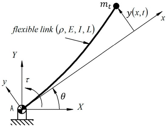
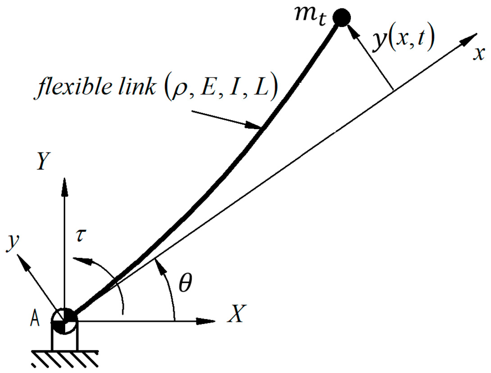
Different modeling approaches have been developed for flexible manipulator systems [28,29]. A flexible manipulator with a single link that is rigidly attached to a rotating hub is considered in this study, as illustrated in Figure 1. Since the manipulator operates in the horizontal plane, gravitational effects are not considered.

Figure 1. Model and description of a single flexible link manipulator system.

The governing equation of motion of the flexible link manipulator can be expressed by the following partial differential equation [30,31,32]:

$$EI{\displaystyle \frac{{\partial }^{4}y\left(x,t\right)}{\partial x^4}}+c\left(x\right){\displaystyle \frac{\partial y\left(x,t\right)}{\partial t}}+\rho {\displaystyle \frac{{\partial }^{2}y\left(x,t\right)}{\partial t^2}}=-\rho x\ddot{\theta }\left(t\right)$$

(1)

The transverse displacement can be expressed using modal expansion as

$$y\left(x,t\right)={\displaystyle \sum _{j=1}^n}{\varnothing }_j\left(x\right)q_j\left(t\right)$$

(2)

where $y\left(x,t\right)$ is the cumulative deflection of a point along the link at a distance $x$ from the axis of rotation, and $E$ is the modulus of elasticity, $I$ is the area moment of inertia, $\rho$ is the mass per unit length of the link, $\theta \left(t\right)$ is the angular displacement, ${\varnothing }_j\left(x\right)$ are the $j$th mode shape, $q_j\left(t\right)$ is the $j$th generalized coordinate, $j$ is the normal mode number, and $m_t$ is the mass of the payload.

It should be noted that the derivation of Equation (1) is based on several simplifying assumptions. The inertia of the hub is considered negligibly small, the beam density and area moment of inertia are assumed to remain constant along the length of the manipulator, and the flexible link is modeled as a Euler–Bernoulli beam. In addition, any centripetal forces arising from rotation are neglected. With these assumptions in place, the boundary conditions can be introduced and the resulting boundary value problem solved to obtain the eigenfunctions, as given in [30,31,33]:

$${\varnothing }_j\left(x\right)=C_j\left[cosh\left({\displaystyle \frac{{\beta }_{j}x}{L}}\right)-cos\left({\displaystyle \frac{{\beta }_{j}x}{L}}\right)-{\gamma }_j\left(sinh\left({\displaystyle \frac{{\beta }_{j}x}{L}}\right)-sin\left({\displaystyle \frac{{\beta }_{j}x}{L}}\right)\right)\right]$$

(3)

where

$${\gamma }_j={\displaystyle \frac{cosh\left({\beta }_j\right)+cos\left({\beta }_j\right)}{sinh\left({\beta }_j\right)+sin\left({\beta }_j\right)}}$$

(4)

and modal amplitude, $C_j$, is to be evaluated by normalizing the eigenfunctions according to the orthogonality conditions:

$$C_j={\left[{\displaystyle \frac{1}{\rho {\displaystyle {\int }_0^L}{{\varnothing }_j}^2\left(x\right)dx+m_t{{\varnothing }_j}^2\left(L\right)}}\right]}^{{\displaystyle \raisebox{1ex}{$1$}\!\left/ \!\raisebox{-1ex}{$2$}\right.}}$$

(5)

where $m_t$ is the mass of the payload. Substituting Equation (2) into Equation (1) and projecting the resulting expression onto the jth mode shape yields the modal equation of motion. The contribution of the tip mass at x = L is included together with the distributed mass of the flexible link. Using the orthogonality of the mode shapes and the normalization defined in Equation (5), the generalized mass of each mode becomes unity. The equation of motion for the jth mode can therefore be expressed as [30,31]:

$${\ddot{q}}_j(t)+ 2{\zeta \omega }_j{\dot{q}}_j(t) +{\omega }_j^2{q}_j(t)={\Lambda }_j\ddot{\theta }\left(t\right)$$

(6)

where ${\omega }_j$ is the $j$th natural frequency, which is given by ${\omega }_j={\beta }_j^2\sqrt{EI/\rho L^4}$ where ${\beta }_j$ is the dimensionless eigenvalue. For a flexible link with a concentrated tip mass $m_t$, the eigenvalues are obtained from the characteristic equation

$$1+cos{\beta }_{j}cosh{\beta }_j+{\beta }_j{\displaystyle \frac{m_t}{\rho L}}\left(cos{\beta }_{j}sinh{\beta }_j-sin{\beta }_{j}cosh{\beta }_j\right)=0$$

(7)

$\mathsf{\Lambda }$ is the ratio of the mode participation scale to the generalized mass:

$${\Lambda }_j=-\rho {\displaystyle \underset{0}{\overset{L}{\int }}}x{\varnothing }_j\left(x\right)dx-m_t{L\varnothing }_j\left(L\right)$$

(8)

The largest vibration amplitudes are generally associated with the first mode, since the beam is primarily excited by distributed inertial forces associated with the prescribed acceleration. In the present study, the motion design therefore focuses on the dominant first vibration mode, consistent with the observations reported in [24,34]. Higher-mode effects are not explicitly included in the present formulation. Extension to a multi-mode system would require additional suppression conditions associated with the corresponding modal frequencies.

Accordingly, Equation (6) is reduced to the dominant first-mode model as

$$\ddot{q}{\left(t\right)+2{\zeta \omega }_n\dot{q}\left(t\right)+\omega }_n^{2}q(t)=\Lambda a\left(t\right)$$

(9)

where $a\left(t\right)$ is the angular acceleration profile.

4. Motion Profile Design and Tuning

This section presents the formulation and tuning of the proposed motion profile. The motion design procedure is derived for both undamped and underdamped systems, and different design scenarios are considered depending on the specified motion parameters. The effectiveness of the proposed approach is then evaluated in comparison with commonly used motion profiles.

4.1. Motion Profile Formulation

Acceleration and deceleration phases are typically incorporated into point-to-point motion profiles to suppress residual vibrations in mechanical systems. In this study, a new approach is proposed for generating and tuning acceleration profiles so that vibration can be reduced effectively over a wide range of motion durations. The motion profile is constructed by superimposing three components: a ramp, a cycloid, and a ramped-versine function, following the general concept introduced for elastic systems in [15]. The amplitudes of these components are determined according to the required displacement, total travel time, and relevant system parameters. While the component relations retain the analytical structure introduced in [15], they are used differently in the two approaches. In [15], the components are used to construct a preshaped reference position command, which is subsequently convolved with modal impulse shapers. In the present method, the tuning is performed directly at the acceleration level, and the resulting acceleration profile defines the prescribed motion without a subsequent impulse-shaping or convolution stage. The motion is divided into four segments.

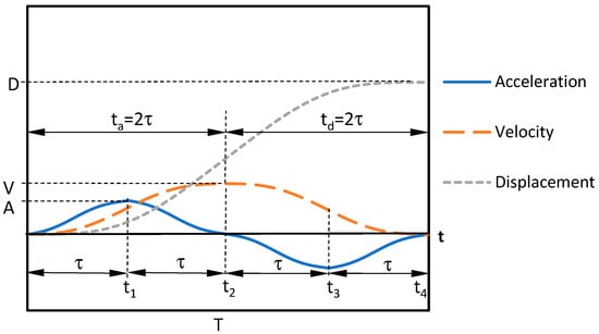
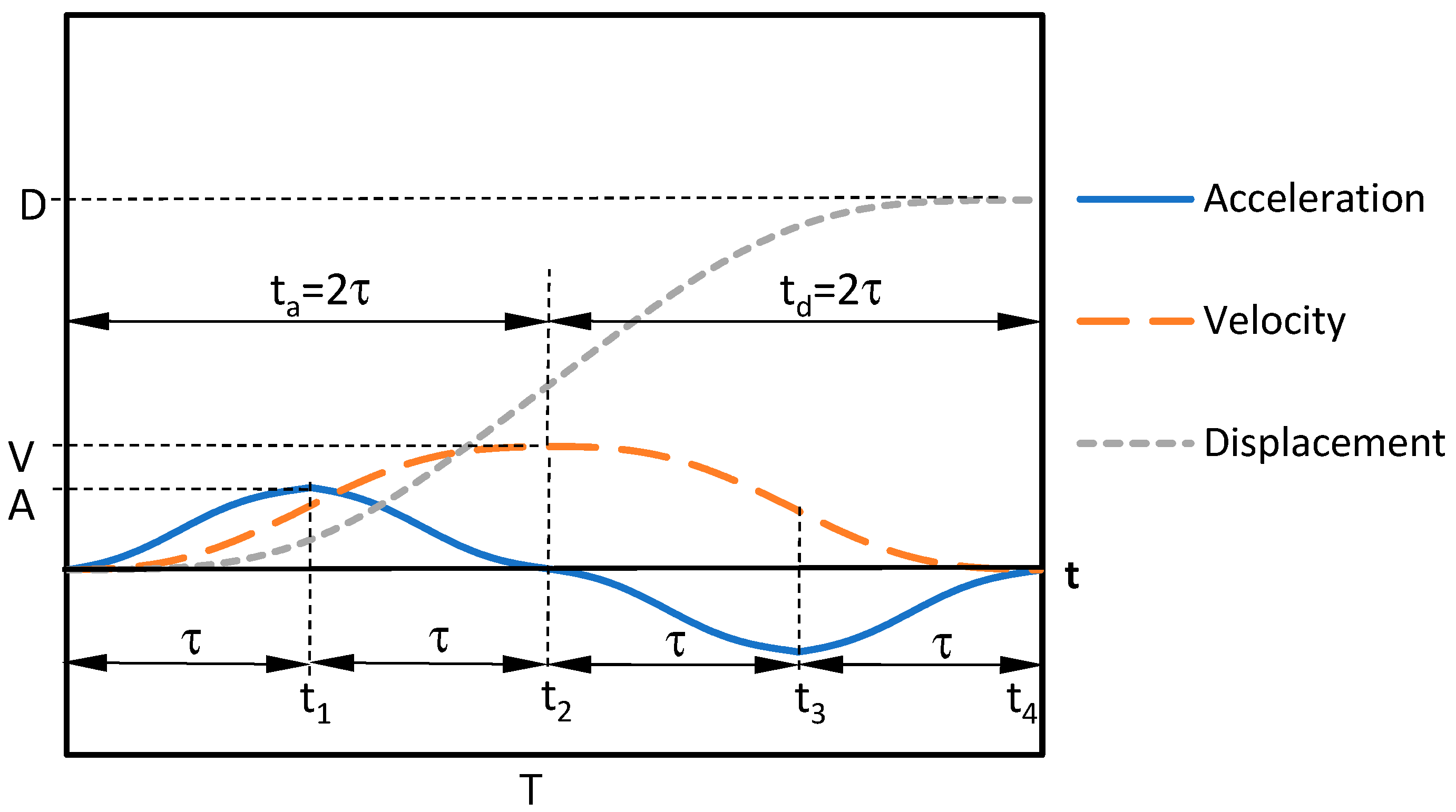
The displacement, velocity, and acceleration corresponding to the proposed motion profile are shown schematically in Figure 2. For a given total travel time T, the motion consists of two main phases: an acceleration phase lasting $t_a=T/2$ and a deceleration phase of equal duration, $t_d=T/2$.

Figure 2. For a given total travel time, $\mathit{T}=\mathbf{4}\mathit{\tau }$, displacement, $\mathit{D}=\mathbf{1} \mathbf{u}\mathbf{n}\mathbf{i}\mathbf{t}$, damping coefficient, $\mathit{\zeta }=\mathbf{0.1}$, and natural frequency ${\mathit{\omega }}_{\mathit{n}}=\mathbf{2}\mathit{\pi }$, the displacement, velocity, and acceleration of the proposed motion profile.

The acceleration phase itself is divided into two parts. During the first half, the acceleration gradually increases; during the second half, it decreases and returns to its initial value. Each of these intervals has a duration of $\tau =T/4$. The deceleration phase follows the same structure, with the magnitude of deceleration first increasing and then returning smoothly to its initial level over two equal subintervals.

The corresponding velocity and displacement profiles are obtained by integrating the acceleration function. When constructing these curves, several conditions must be satisfied. The total motion time must equal the sum of the acceleration and deceleration phases $(T=t_a+t_d$), the velocity should remain continuous at the junctions between segments, and the transitions must avoid infinite jerk [35]. To achieve a smooth motion profile, the acceleration in each segment is described using a combination of ramp, cycloidal, and ramped-versine components. The ramp component introduces a gradual change in acceleration with bounded jerk, allowing the motion to start smoothly and helping to limit high-frequency excitation of the flexible structure. The cycloidal component is included to maintain smooth velocity and acceleration transitions while preventing abrupt variations in jerk, a characteristic that has been widely utilized in precision motion design. The ramped-versine component provides a smooth harmonic variation in acceleration, which is well suited for shaping the modal response of flexible systems and thereby reducing residual vibrations.

General form of the acceleration profile is expressed as

$$a\left(t\right)={\displaystyle \frac{A_{1}Rt}{2\pi }}+{\displaystyle \frac{A_2}{2\pi }}\left[Rt-sin\left(Rt\right)\right]+{\displaystyle \frac{A_3}{2\pi }}\left[1-cos\left(Rt\right)\right]+{\displaystyle \frac{A_3}{2\pi }}Rt$$

(10)

where $A_1$ represents the amplitude of a ramp profile, $A_2$ denotes the amplitude of a cycloid motion profile, $A_3$ the amplitude of a ramped-versine motion profile. $t$ signifies time into motion,$\tau$ is the segment duration for each section, and $R=2\pi /\tau$. Furthermore, summation of these amplitudes gives the acceleration-amplitude parameter ${A=A}_1+A_2+A_3$. Rearranging the equations yields:

$$a\left(t\right)={\displaystyle \frac{ARt}{2\pi }}-{\displaystyle \frac{A_2}{2\pi }}sin\left(Rt\right)+{\displaystyle \frac{A_3}{2\pi }}\left[1-cos\left(Rt\right)\right]$$

(11)

where $A_1$, $A_2$, and $A_3$ are tuned using the overall acceleration, the duration of each section, $\tau$. The response of the system described by Equation (9) after the completion of the maneuver ($t\ge 4\tau =T$) can be expressed as

$$q=e^{-\zeta w_n\left(t-T\right)}\left[C_1\mathit{sin}{w}_d\left(t-T\right)+C_2\mathit{cos} w_d\left(t-T\right)\right]$$

(12)

In this expression, the constants $C_1$ and $C_2$ determine the coefficients of the post-maneuver free-vibration response. For zero residual vibration, both coefficients must vanish simultaneously,

$$C_1=0, C_2=0$$

These conditions are equivalent to requiring the modal displacement and velocity to vanish at the end of the maneuver,

$$q\left(t\right)=0 \mathit{and} \dot{q}\left(t\right)=0.$$

these two terminal conditions can be expressed by the complex zero-residual condition

$$\int a\left(t\right)e^{st}dt=0$$

where

$$s=\zeta w_n+i{w}_{d }{w}_d=w_n\sqrt{1-{\zeta }^2}$$

The complex parameter s satisfies the characteristic equation of the underdamped system,

$$s^2-2\zeta w_{n}s+w_n^2=0$$

Substituting the complete four-segment acceleration profile into the zero-residual condition, with T = 4τ and R = 2π/τ, and simplifying the resulting expression using the symmetry of the acceleration and deceleration phases gives

$$(A-A_2)s^2-A_{3}Rs+A{R}^2=0$$

Dividing by $A-A_2$ yields

$$s^2-{\displaystyle \frac{A_{3}R}{A-A_2}}s+{\displaystyle \frac{A{R}^2}{A-A_2}}=0$$

Comparison with the characteristic equation gives the following two conditions:

$${\displaystyle \frac{A_{3}R}{A-A_2}}=2\zeta w_{n }{\displaystyle \frac{A{R}^2}{A-A_2}}=w_n^2$$

Therefore,

$$A_1={\displaystyle \frac{AR\left(R-2\zeta {\omega }_n\right)}{{\omega }_n^2}}={\displaystyle \frac{A{\tau }_n\left({\tau }_n-2\zeta \tau \right)}{{\tau }^2}}$$

(13)

$$A_2=A\left(1-{\displaystyle \frac{R^2}{{\omega }_n^2}}\right)=A\left(1-{\displaystyle \frac{{\tau }_n^2}{{\tau }^2}}\right)$$

(14)

and

$$A_3={\displaystyle \frac{A2\zeta R}{{\omega }_n}}={\displaystyle \frac{A2\zeta {\tau }_n}{\tau }}$$

(15)

Here, ${\omega }_n$, ${\tau }_n$, $\zeta$ represent the natural frequency of the first vibration mode, the first mode period of the system and the first mode damping ratio to suppress the residual vibration, respectively.

The fundamental principle of this method is that each individual motion component $(A_1,A_2{, A}_3)$ induces its own set of oscillations within the system. When the amplitudes of these functions are precisely selected according to the expressions above, the modal responses generated by the three components cancel each other through superposition. As a result, the system reaches the desired position without residual vibration. It is worth emphasizing that the suppression of residual vibration is not achieved simply by mirroring the acceleration profile given in Figure 2. Instead, the amplitudes of the ramp, cycloid, and ramped-versine components are determined analytically so that the modal response coefficients of the free vibration solution become zero at the end of the maneuver. In this way, the residual vibration terms vanish even when damping is present.

The parameter A is an acceleration-amplitude parameter used in constructing the four-segment motion profile, whereas the actual peak acceleration is determined from the resulting complete profile. In practice, achieving shorter maneuver durations generally requires higher acceleration and jerk levels, which is a common consideration in high-speed positioning systems. The proposed formulation provides the motion profile required for vibration suppression, whereas its practical implementation depends on the capabilities of the available actuator and transmission system.

One of the main advantages of the proposed tuned command is that, in theory, it does not impose a specific constraint on the total travel time. The only limiting case occurs when $\tau$ approaches zero, which is not physically meaningful in practice.

For $t\in \left[0, t_1\right]$, Equation (16) defines the first segment, which begins with zero acceleration.

$$a\left(t\right)={\displaystyle \frac{ARt}{2\pi }}-{\displaystyle \frac{A_2}{2\pi }}sin\left(Rt\right)+{\displaystyle \frac{A_3}{2\pi }}\left[1-cos\left(Rt\right)\right]$$

(16)

For $t\in \left[t_1, t_2\right]$, Equation (17) defines the second segment, which connects continuously to the first and reaches zero acceleration at ${t=t}_2$.

$$a\left(t\right)=A-\left({\displaystyle \frac{AR(t-t_1)}{2\pi }}-{\displaystyle \frac{A_2}{2\pi }}sin\left(R\left(t-t_1\right)\right)+{\displaystyle \frac{A_3}{2\pi }}\left[1-cos\left(R\left(t-t_1\right)\right)\right]\right)$$

(17)

For $t\in \left[t_2, t_3\right]$, Equation (18) defines the third segment, which begins with zero acceleration at ${t=t}_2$.

$$a\left(t\right)=-\left({\displaystyle \frac{AR(t-t_2)}{2\pi }}-{\displaystyle \frac{A_2}{2\pi }}sin\left(R\left(t-t_2\right)\right)+{\displaystyle \frac{A_3}{2\pi }}\left[1-cos\left(R\left(t-t_2\right)\right)\right]\right)$$

(18)

For $t\in \left[t_3, t_4\right]$, Equation (19) defines the fourth segment, which connects continuously to the third and returns to zero acceleration at the end of the motion.

$$a\left(t\right)=-A+\left({\displaystyle \frac{AR(t-t_3)}{2\pi }}-{\displaystyle \frac{A_2}{2\pi }}sin\left(R\left(t-t_3\right)\right)+{\displaystyle \frac{A_3}{2\pi }}\left[1-cos\left(R\left(t-t_3\right)\right)\right]\right)$$

(19)

The corresponding velocity profiles can be obtained by integrating Equations (16)–(19) with respect to time, while the displacement profiles follow from a second integration of the same expressions. The acceleration is continuous at all segment boundaries by construction. The jerk remains finite throughout the motion and is continuous at the central boundary t = t₂. At the boundaries t = t₁ and t = t₃, jerk continuity requires A₂ = A; otherwise, finite changes in jerk occur at these boundaries. The maximum jerk magnitude of the four-segment profile is $j_{\mathrm{m}\mathrm{a}\mathrm{x}}=(A+\sqrt{A_2^2+A_3^2})/\tau$. As the segment duration decreases, the jerk level generally increases, resulting in greater high-frequency content in the command and a higher potential for excitation of higher flexible modes.

Depending on the damping characteristics of the system, two design cases are considered: undamped and underdamped systems.

4.2. Motion Design for Undamped Systems $\left(\zeta =0\right)$

In the undamped case, the ramped-versine component is not required. i.e., $A_3=0$. The displacement at the end of the complete four-segment motion is given by:

$$D=2A{\tau }^2$$

(20)

For a given total travel time $T=4\tau$ and prescribed displacement $D$, the acceleration-amplitude parameter $A$ can be calculated as

$$A={\displaystyle \frac{8D}{T^2}}$$

(21)

4.3. Motion Design for Underdamped Systems

For underdamped systems, the motion design problem becomes more involved, since damping influences the system response and the ramped-versine component plays a role in shaping the acceleration profile.

Considering the proposed acceleration profile, the velocity and displacement relations can be obtained by integration. The velocity reached at $t_2$ is given by

$$v\left(t_2\right)=V=A\tau$$

(22)

At the end of the motion $t_4$, the displacement reaches the desired value:

$$d\left(t_4\right)=D={\tau }^2\left({\displaystyle \frac{32{\pi }^{3}A-A_3}{16{\pi }^3}}\right)$$

(23)

For a prescribed displacement $D$ and total travel time $T=4\tau$, the acceleration-amplitude parameter $A$ can be obtained by substituting the ramped-versine amplitude given in Equation (15) into Equation (23).

$$A={\displaystyle \frac{16{\pi }^2{\omega }_{n}D}{T\left(2{\pi }^{2}T{\omega }_n-\zeta \right)}}$$

(24)

4.4. Comparison with Existing Motion Profiles

The proposed motion profiles are evaluated by comparing their performance with that of previously reported S-curve motion profiles, focusing on their ability to eliminate residual vibration. Earlier studies have identified specific conditions under which trapezoidal [20,22] and trigonometric profiles [21] can achieve vibration suppression. It is also well known that, regardless of the form of the input function, residual vibration can be eliminated when the motion duration is selected in relation to the natural period of the damped system [20,23,36,37,38]. Several works have confirmed that choosing motion times close to the system’s natural period significantly reduces residual vibrations.

The results of the present study show that effective vibration suppression can be achieved without restricting the motion duration to integer or half-integer multiples of the natural period. In this sense, the proposed approach provides greater flexibility in selecting motion times.

5. Experimental Set-Up, Data Collection and Numerical Simulation

The modal equation of motion was integrated using the fourth-order Runge–Kutta method with a fixed time step of 0.001 s in numerical simulations. The simulations considered the dominant first vibration mode of the flexible link, with zero initial modal displacement and velocity, $q\left(0\right)=0$ and $\dot{q}\left(0\right)=0$. Damping was represented by the viscous modal damping term $2\zeta {\omega }_n$, with $\zeta =0$ for the undamped case and the experimentally identified damping ratio for the underdamped case.

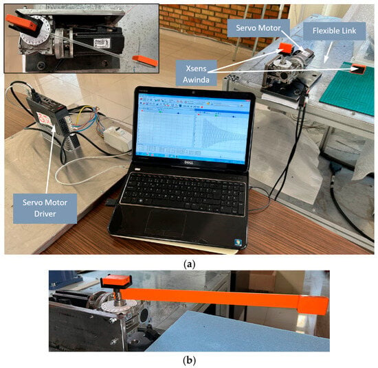
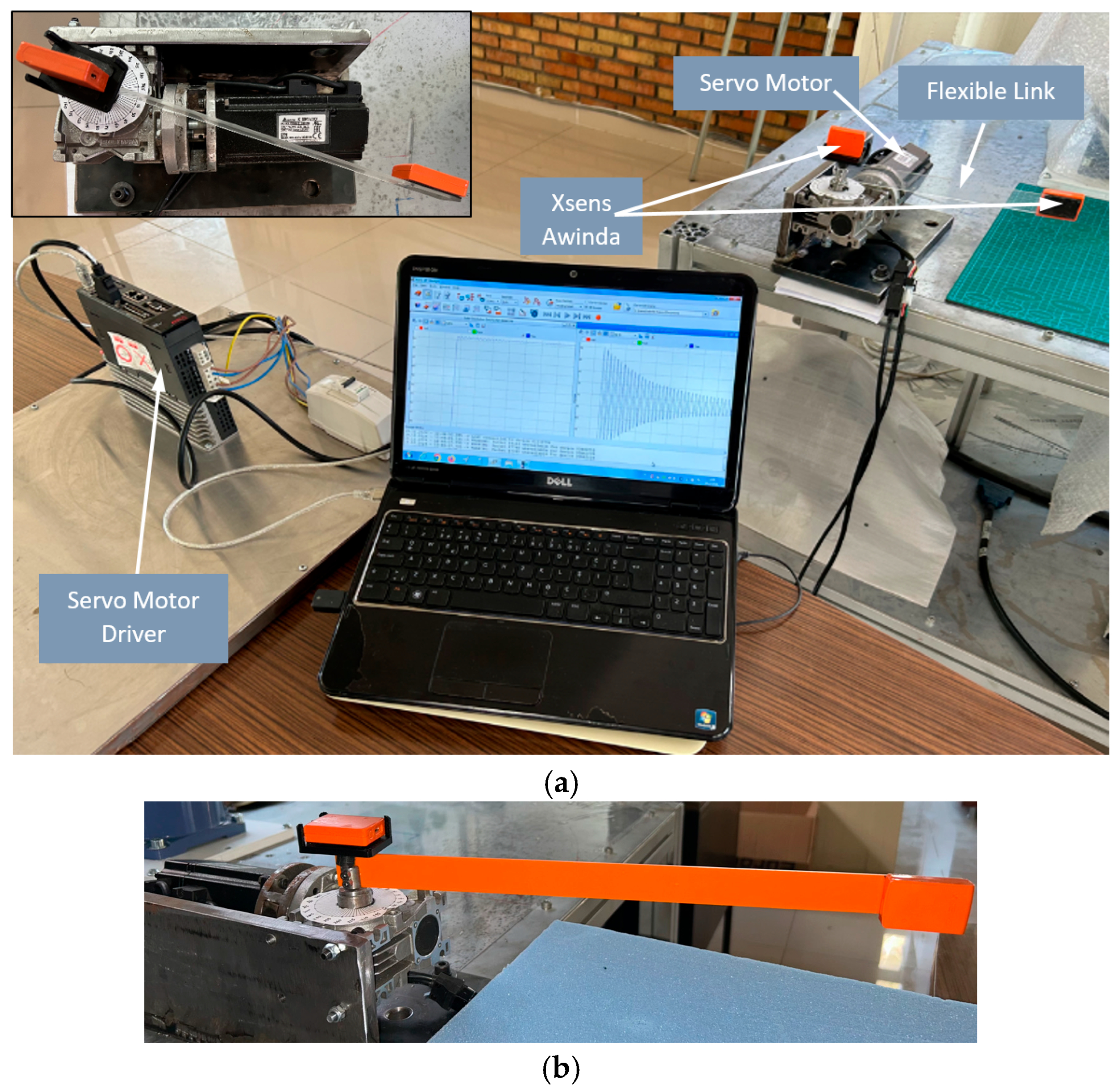
The experimental setup shown in Figure 3a consisted of an ASDA-A2 Delta servo motor [39] driving a single-link flexible manipulator through a gearbox with a reduction ratio of 1:28. The motor was operated in position control mode. Reference motion profiles were generated offline and then uploaded to the controller using the ECAM functionality. The dynamics of the servo drive, its internal controller, and the gearbox were not included in the numerical model; instead, the prescribed motion was applied directly to the flexible-link model. In the experiments, the gearbox reduction ratio was taken into account when defining the commanded motion in the servo interface.

Figure 3. Experimental setup and flexible links used in the experiments: (a) experimental setup with Flexible Link 1; (b) Flexible Link 2.

Vibration measurements were obtained using two Xsens MTw Awinda inertial measurement units (IMUs) [40]. One sensor was mounted at the tip of the flexible link, while the other was placed near the axis of rotation, as shown in Figure 3a. The signals from both IMUs were recorded simultaneously using MT Manager (version 2022.2) software at a sampling rate of 100 Hz. The base-mounted IMU was used to determine the actual beginning and end of the hub motion and to verify the prescribed (22.5°) rotation and motion duration, whereas the tip-mounted IMU was used to measure the vibration response of the flexible link. According to the mounting orientation of the tip IMU, the yaw (heading) angle was used as the measured vibration coordinate. The tip-mounted IMU directly measures angular motion rather than transverse displacement. Therefore, the measured yaw angle was converted to the corresponding tip displacement using the established angle-to-displacement relationship based on the dominant first-mode shape. This allowed the experimental response to be expressed in the same displacement units as the response obtained from the dynamic model. The experiments were repeated under the same operating conditions in a controlled laboratory environment. Each MTw sensor has a mass of approximately 16 g. The mass of the tip-mounted IMU was included as part of the concentrated tip mass mt in the dynamic model, thereby accounting for its contribution to the dynamic properties of the experimental system. According to the manufacturer specifications, the MTw Awinda provides a dynamic heading accuracy of 1.5° RMS and a static heading accuracy of 1.0° RMS.

Data acquisition was initiated before the prescribed motion and continued after its completion for a sufficient duration to capture the subsequent free-vibration response. Since both IMUs were recorded simultaneously, the beginning and end of the actual hub motion identified from the base-mounted IMU were used to define the corresponding time interval in the tip response. This interval was considered the transient motion region, whereas the response following completion of the hub motion was considered the post-maneuver residual-vibration region. The maximum and minimum values of the first oscillation in the post-maneuver response were identified, and the residual-vibration amplitude was calculated as half of the corresponding peak-to-peak value. Since different normalized motion durations were investigated, the total recording duration was not fixed across the experiments.

Two different flexible links were used in the experiments, as shown in Figure 3a,b. The first link (Link 1) exhibited negligible damping and was therefore treated as undamped, whereas the second link (Link 2) showed noticeable damping and was considered underdamped. The geometric and material properties of these links, corresponding to the model presented in Figure 1, are summarized in Table 1.

Table 1. Geometric and material properties of the flexible links used in the experiments.

Parameter	Description	Link 1	Link 2
L	Length of flexible link	0.295 m	0.36 m
E	Young’s modulus of elasticity	3 GPa	3 GPa
I	Area moment of inertia	2.79 × 10−11 m4	4.518 × 10−11 m4
ρ	Mass per unit length	0.0597 kg/m	0.07694 kg/m
Ac	Cross-sectional area of the link	5.81 × 10−5 m2	6.916 × 10−5 m2
mt	Payload mass	16 × 10−3 kg	16 × 10−3 kg

The dynamic parameters of the two links were determined from their free-vibration responses. The natural frequencies were experimentally identified using Fast Fourier Transform (FFT) analysis, while the damping ratio, ζ, was estimated from successive peaks of the free-decay response using the logarithmic decrement method. For Flexible Link 1, the first and second natural frequencies were identified as 27.167 and approximately 270 rad/s (4.32 and 42.97 Hz), respectively. For Flexible Link 2, the corresponding frequencies were 19.654 and approximately 180 rad/s (3.13 and 28.65 Hz), respectively. In addition, the dimensionless eigenvalue β was obtained numerically by solving the characteristic equation using the bisection method, and the corresponding natural frequency was calculated from the analytical model.

6. Performance Evaluation and Experimental Validation of the Proposed Motion Design

Evaluating the effectiveness of different command shaping techniques requires clearly defined performance metrics. Meaningful comparisons should be grounded in quantitative analysis, since objective measures provide a reliable basis for assessing performance. For example, a practical goal might be to reduce the residual vibration to less than 5% of that observed without command shaping, or to minimize the time needed to attenuate vibrations to an acceptable level. For these reasons, a consistent and reliable method for quantifying the level of vibration suppression achieved by a given command shaping strategy is essential.

One practical way to quantify performance is through a slightly modified version of the Percent Residual Vibration (PRV) metric, which is commonly used to evaluate how effectively a method reduces residual vibration [41]. PRV provides a normalized measure by comparing the residual vibration produced by a given vibration-reducing command with the maximum residual amplitude obtained from a reference, or nominal command. In this study, an untuned S-curve command evaluated at a normalized time ratio of $T/{\tau }_n=1$ is selected as the reference profile. Its maximum post-maneuver residual vibration amplitude is used as the baseline in the PRV calculation. For each flexible-link system, a single reference amplitude is used consistently for all motion profiles included in the corresponding comparison.

The PRV values for all other motion commands are then calculated relative to this reference using the following expression:

$$\mathrm{P}\mathrm{R}\mathrm{V}=100\times {\displaystyle \frac{\mathrm{R}\mathrm{e}\mathrm{s}\mathrm{i}\mathrm{d}\mathrm{u}\mathrm{a}\mathrm{l} \mathrm{v}\mathrm{i}\mathrm{b}\mathrm{r}\mathrm{a}\mathrm{t}\mathrm{i}\mathrm{o}\mathrm{n} \mathrm{o}\mathrm{f} \mathrm{p}\mathrm{r}\mathrm{o}\mathrm{p}\mathrm{o}\mathrm{s}\mathrm{e}\mathrm{d} \mathrm{c}\mathrm{o}\mathrm{m}\mathrm{m}\mathrm{a}\mathrm{n}\mathrm{d}}{\mathrm{M}\mathrm{a}\mathrm{x}\mathrm{i}\mathrm{m}\mathrm{u}\mathrm{m} \mathrm{r}\mathrm{e}\mathrm{s}\mathrm{i}\mathrm{d}\mathrm{u}\mathrm{a}\mathrm{l} \mathrm{v}\mathrm{i}\mathrm{b}\mathrm{r}\mathrm{a}\mathrm{t}\mathrm{i}\mathrm{o}\mathrm{n} \mathrm{o}\mathrm{f} \mathrm{s}\mathrm{e}\mathrm{l}\mathrm{e}\mathrm{c}\mathrm{t}\mathrm{e}\mathrm{d} \mathrm{n}\mathrm{o}\mathrm{m}\mathrm{i}\mathrm{n}\mathrm{a}\mathrm{l} \mathrm{c}\mathrm{o}\mathrm{m}\mathrm{m}\mathrm{a}\mathrm{n}\mathrm{d}}}$$

(25)

The calculated PRV values are plotted as a function of the normalized time ratio, which represents the ratio between the total command duration and the system’s natural period. Presenting the results in this way allows the performance of different command shapers to be evaluated on a common basis. As a result, their behavior can be compared more consistently under varying operating conditions.

Numerical simulations were carried out to evaluate the effectiveness of the proposed motion tuning method in reducing or eliminating residual vibrations in the system described by Equation (9). The simulations were performed using the proposed acceleration profile and were designed to provide a clear comparison with both untuned motion and other commonly used profiles. For this purpose, several representative acceleration profiles from the literature were considered. These included the trapezoidal commands reported by Kim et al. [21], Yavuz et al. [23], and Akdağ and Şen [22]; the trigonometric profile proposed by Kim et al. [21]; the cycloidal profile introduced by Ankaralı and Diken [42]; and the constant acceleration profile, along with its modified version based on the first three Fourier terms, as presented by Alnefai et al. [9]. The comparison was performed by prescribing the same displacement and total travel time for each motion profile.

6.1. Undamped System

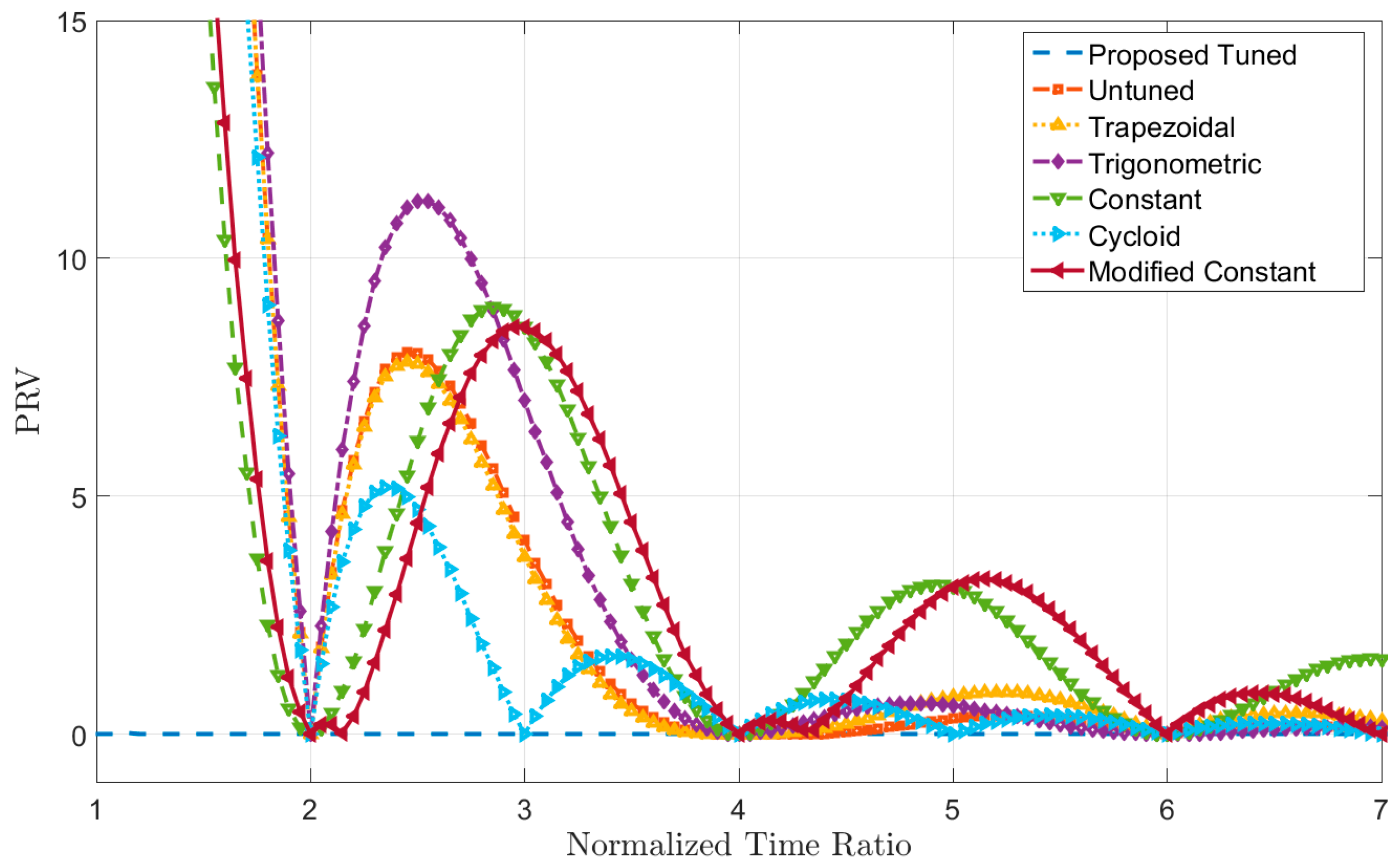
In this case, Equation (11) was selected as the nominal command. $A_2$ was arbitrarily set to $0.5\mathrm{A}$ to obtain a smooth S-curve profile. Based on numerical simulations, the maximum residual vibration associated with this command was found to be 0.05315 m when the normalized time ratio was set to $T/{\tau }_n=1$. The variation in PRV with respect to the normalized time ratio is shown in Figure 4. For the first flexible link, the first-mode natural frequency was measured as ${\omega }_n=27.167$ rad/s, and the corresponding damping ratio was $\zeta = 0.0085$ with ${\beta }_1=1.2719$. Since the measured damping was very small and the associated amplitude decay occurred slowly compared to the time scales considered, the system was treated as undamped in the simulations. Accordingly, the damping ratio was set to zero in the numerical model.

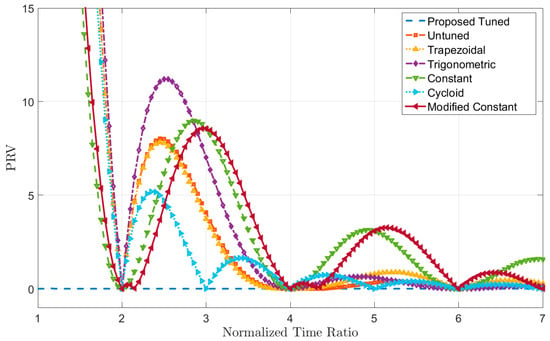
Figure 4. Comparison of the residual-vibration suppression performance of the considered motion profiles for the undamped system. Reference profiles: trapezoidal [21,22,23], trigonometric [21], constant and modified constant [9], and cycloidal [42].

With the exception of the cycloidal command, the other motion profiles yield zero residual vibration when the normalized time ratio is selected as an even integer $({\displaystyle \frac{T}{{\tau }_n}} \ge 2n, n \in \mathbb{Z})$. The cycloidal profile follows a slightly different pattern: it achieves zero residual vibration when the time ratio is an odd integer greater than two. For most of the proposed commands, the PRV falls below 1% once the time ratio exceeds four, with the constant acceleration and its modified Fourier-based version being the main exceptions. This behavior is consistent with a well-known result: regardless of the specific profile shape, if the transient motion duration is chosen as an even multiple of the system’s natural period, the residual vibration becomes negligible. From a practical perspective, once the PRV drops below approximately 5%, further increasing the motion duration offers little benefit. Extending the motion time beyond that point merely lengthens the overall process without yielding a meaningful additional reduction in vibration.

The proposed method yields lower PRV values than the other commands presented in Figure 4 over the investigated range of normalized time ratios, with the PRV remaining close to zero. Low PRV values are also maintained for normalized time ratios below 2. In this region, where many conventional profiles begin to show limitations, the proposed approach does not exhibit any inherent theoretical restrictions.

Several important observations can be drawn from Figure 4. As the motion duration increases, the reduction in vibration may increasingly be influenced by the system’s natural damping rather than by the specific characteristics of the motion profile. When this happens, it becomes challenging to determine whether the observed vibration suppression results from the dynamics of the system itself or from the effectiveness of the proposed motion design.

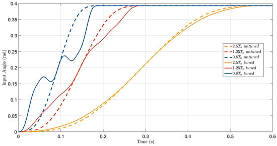
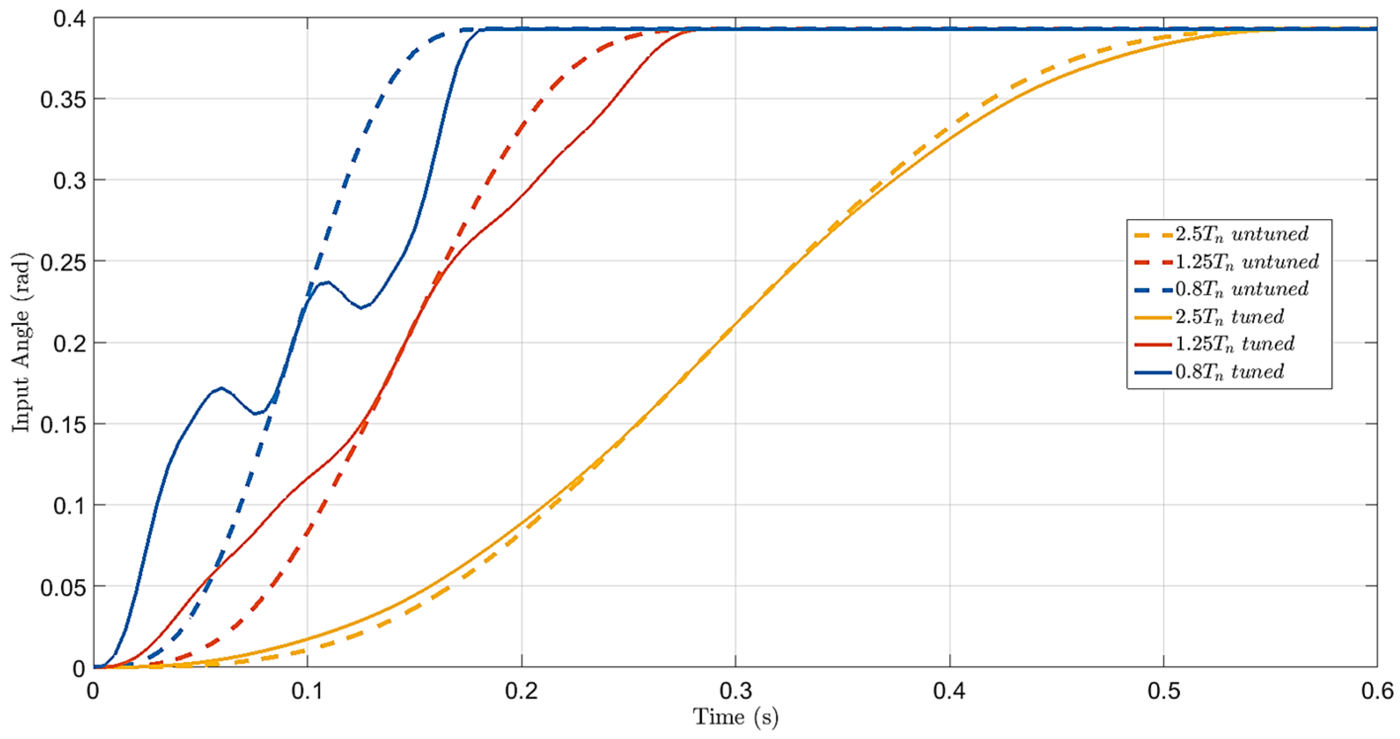
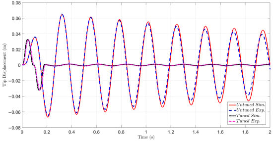
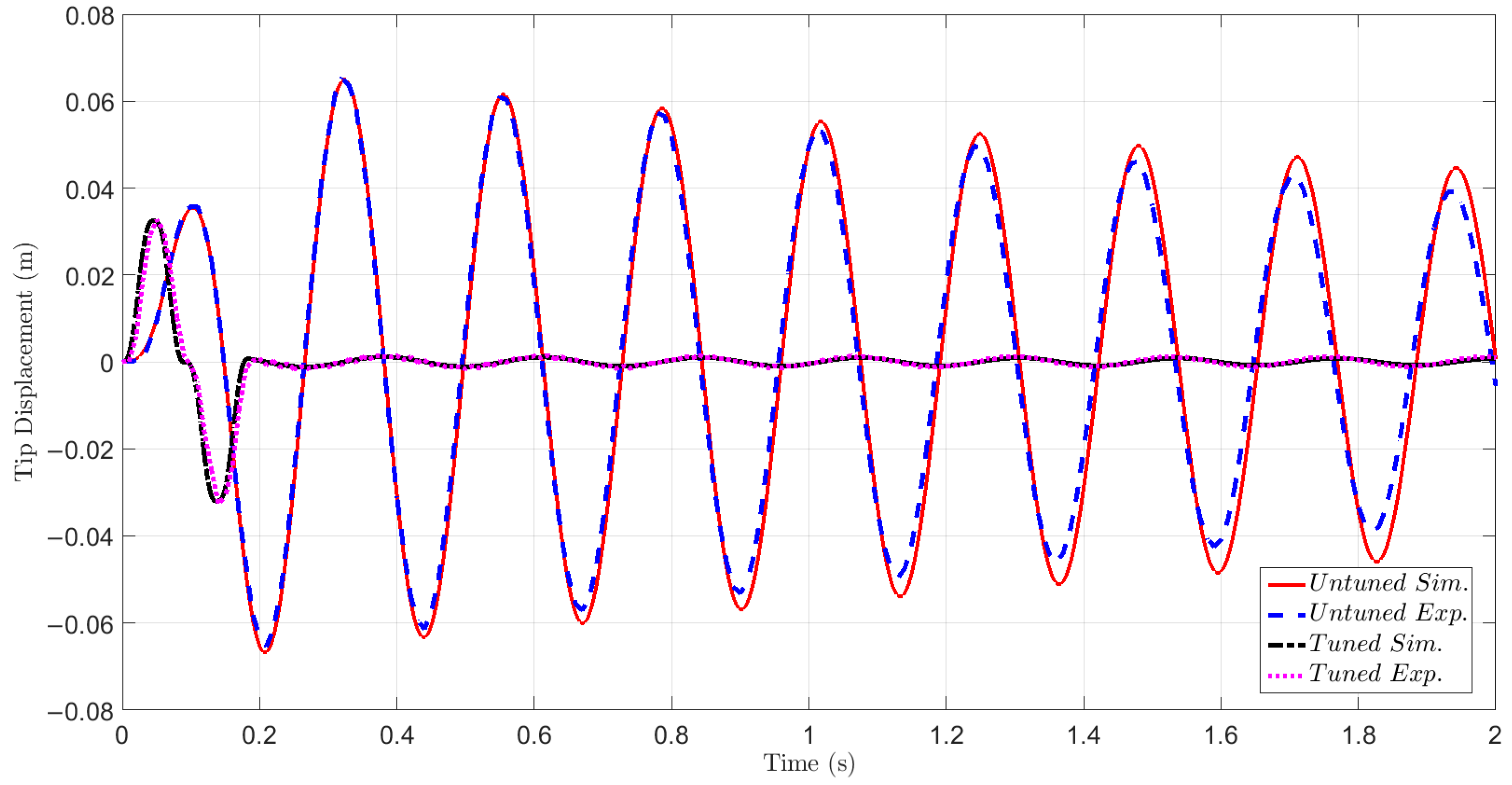
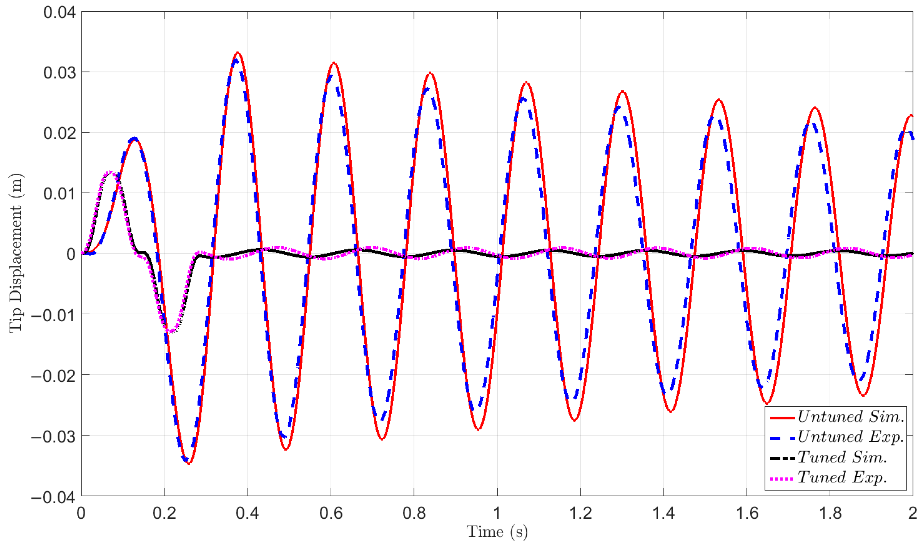
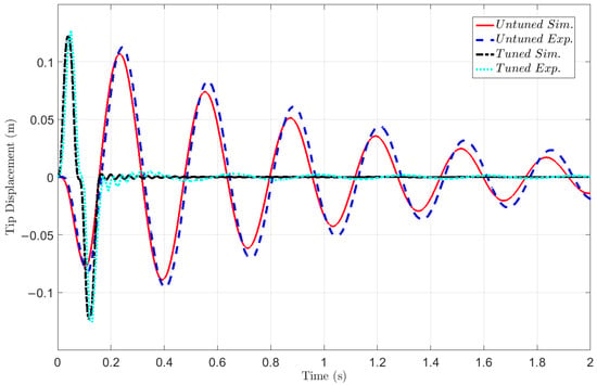
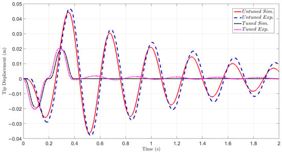
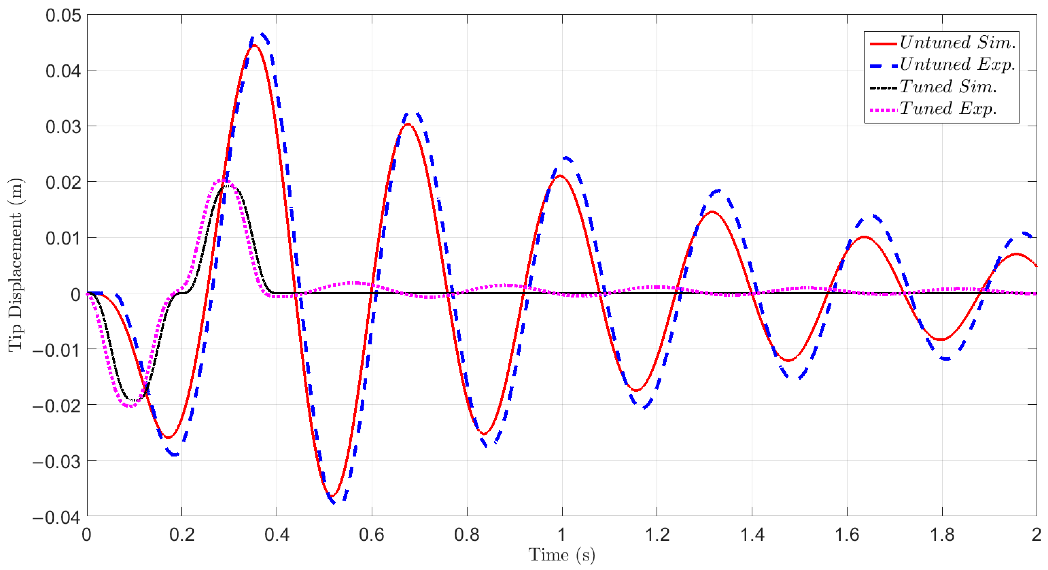
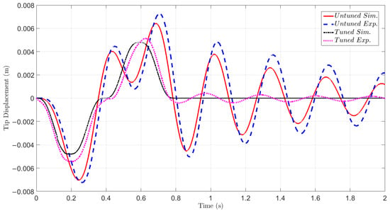
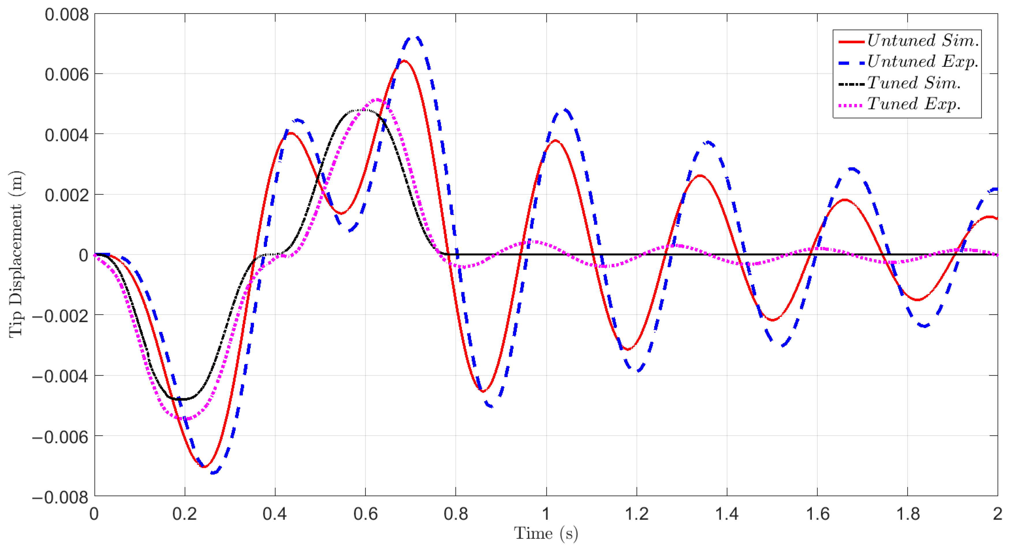
A series of simulations and experiments were carried out to examine the dynamic response of both the untuned and the proposed tuned commands. Three different total motion durations were selected for comparison: $T=0.8{\tau }_n$, $T=1.25{\tau }_n$, $T=2.5{\tau }_n$, with the hub displacement fixed at $D=22.5°$. For each case, the acceleration-amplitude parameter A was calculated using Equation (21). For the untuned profile, the parameter $A_2$ was arbitrarily set to 0.5A, and the remaining expressions were obtained from Equations (16)–(19). In contrast, the proposed tuned acceleration profile was determined by first tuning the relevant parameters through Equations (13) and (15), and then constructing the complete profile using Equations (16)–(19). Figure 5 shows the input angle profiles for the tuned and untuned motions with motion durations equal to $0.8{\tau }_n$, ${1.25\tau }_n$, and $2.5{\tau }_n$. The corresponding simulation and experimental results for both tuned and untuned motions of the undamped link (Link 1) at the selected motion durations are presented in Figure 6, Figure 7 and Figure 8, respectively.

Figure 5. Input angle profiles used for the tuned and untuned motions of the undamped flexible beam.

Figure 6. Simulation and experimental results of tuned and untuned signals for Link 1 at $\mathit{T}=\mathbf{0.8}{\mathit{\tau }}_{\mathit{n}}.$

Figure 7. Simulation and experimental results of tuned and untuned signals for Link 1 at $\mathit{T}=\mathbf{1.25}{\mathit{\tau }}_{\mathit{n}}.$

Figure 8. Simulation and experimental results of tuned and untuned signals for Link 1 at $\mathit{T}=\mathbf{2.5}{\mathit{\tau }}_{\mathit{n}}.$

The maximum residual vibration amplitude was determined from the first oscillation following the completion of the prescribed motion. The maximum and minimum values of this oscillation were identified, and the residual vibration amplitude was calculated as half of the corresponding peak-to-peak value. The simulation and experimental results presented in Figure 6, Figure 7 and Figure 8 clearly show that residual vibration is effectively suppressed for all selected motion durations. This holds true regardless of the selected motion duration. Notably, even when the motion is completed in less than one natural period, a substantial reduction in residual vibration can still be achieved. The corresponding maximum residual vibration amplitudes are listed in Table 2. As anticipated, increasing the total travel time leads to a further decrease in the vibration amplitudes. The experimental motions of Flexible Link 1 under the tuned and untuned commands are provided in the Supplementary Materials.

Table 2. Maximum Residual Vibration Amplitude measured at the tip of Flexible Link 1.

Total Travel Time	Simulation (mm)			Experimental (mm)
	Untuned	Tuned	Reduction (%)	Untuned	Tuned	Reduction (%)
0.8 ${\tau }_n$	64.99	1.14	98.25	65.35	1.53	97.66
1.25 ${\tau }_n$	33.16	0.61	98.16	32.02	0.95	97.03
2.5 ${\tau }_n$	3.99	0.11	97.24	4.60	0.37	91.96

A closer look at Figure 6, Figure 7 and Figure 8 reveals that a small amount of residual vibration remains at the end of the motion in both the simulation and experimental results. Two factors may explain this behavior.

• First, the motion input was designed under the assumption of an undamped system, meaning the damping ratio was taken as zero. In reality, however, the physical system does exhibit a small amount of damping, even if it is very low.
• Second, the motion command is executed through an electromechanical drive system. Minor vibrations at the end of the motion may therefore arise from practical factors such as servo control dynamics or mechanical imperfections in the gearbox connecting the motor to the flexible link.

6.2. Underdamped System

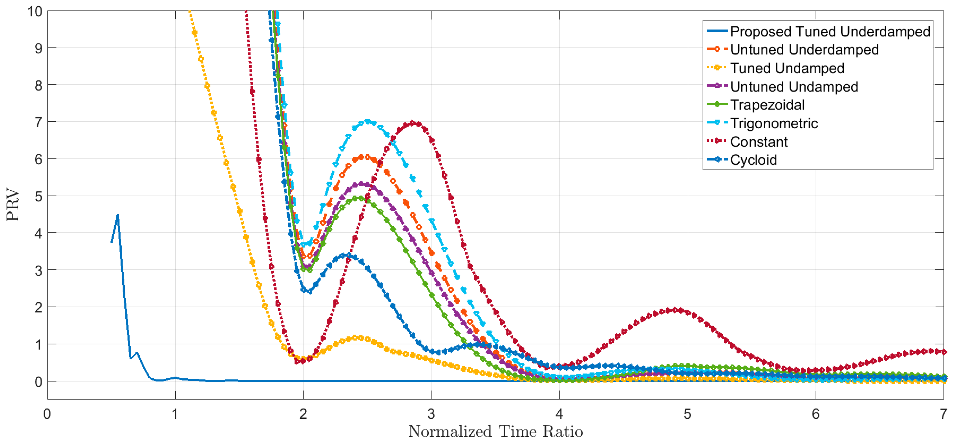
For the second flexible link, the first-mode natural frequency was measured as ${\omega }_n=19.654$ rad/s, with a corresponding damping ratio of $\zeta = 0.05831$. The parameter ${\beta }_1$ was calculated as 1.384368. In this case, Equation (11) was selected as the nominal command, with the amplitudes chosen as ${A_1=A}_2=A_3=\mathrm{A}/3$ to obtain a tuned reference profile. Numerical simulations showed that, for a normalized time ratio of $T/{\tau }_n=1$, the maximum residual vibration associated with this command was 0.0624 m. The variation in PRV with respect to the normalized time ratio is illustrated in Figure 9.

Figure 9. Comparison of the residual-vibration suppression performance of the considered motion profiles for the underdamped system. Reference profiles: trapezoidal [21,22,23], trigonometric [21], constant [9], and cycloidal [42].

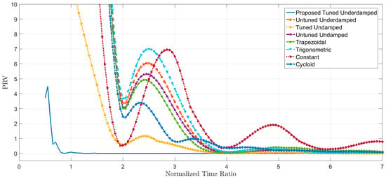
As illustrated in Figure 9, the proposed function performs well even when the underdamped system is approximated as undamped by setting $A_3=0$. In this simplified case, it still yields better results than the other profiles, particularly when the motion duration exceeds twice the natural period. When damping is explicitly taken into account in the formulation, the improvement becomes even more pronounced. Under these conditions, residual vibration is almost completely eliminated once the motion duration reaches roughly 0.8 times the natural period.

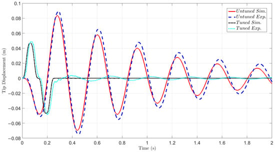
To further examine the dynamic response of both the untuned and tuned commands in the underdamped case, a series of simulations and experiments were carried out. Four different motion durations were selected for comparison: T$=0.5{\tau }_n$, $T=0.8{\tau }_n$, $T=1.25{\tau }_n$, $T=2.5{\tau }_n$. In all cases, the angular displacement of the hub was fixed at $D=22.5°$. For the numerical and experimental evaluation, the tuned command was generated using the proposed underdamped formulation. For each motion duration, the acceleration-amplitude parameter A was determined from Equation (24), and the component amplitudes were calculated using Equations (13)–(15). The complete profile was then constructed using Equations (16)–(19).

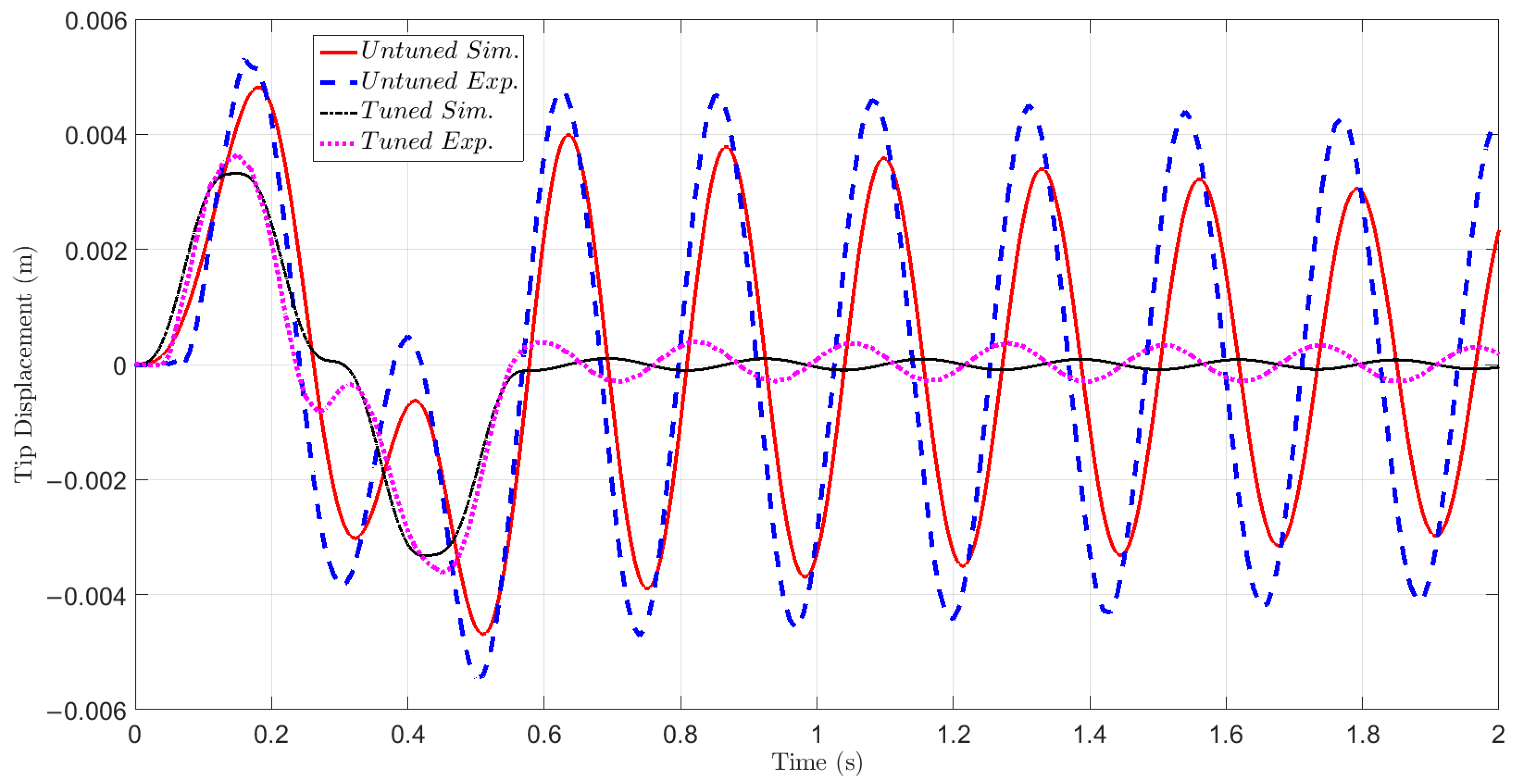
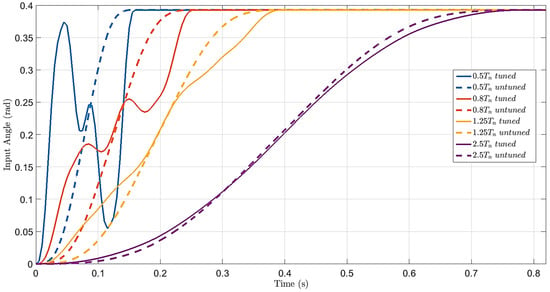
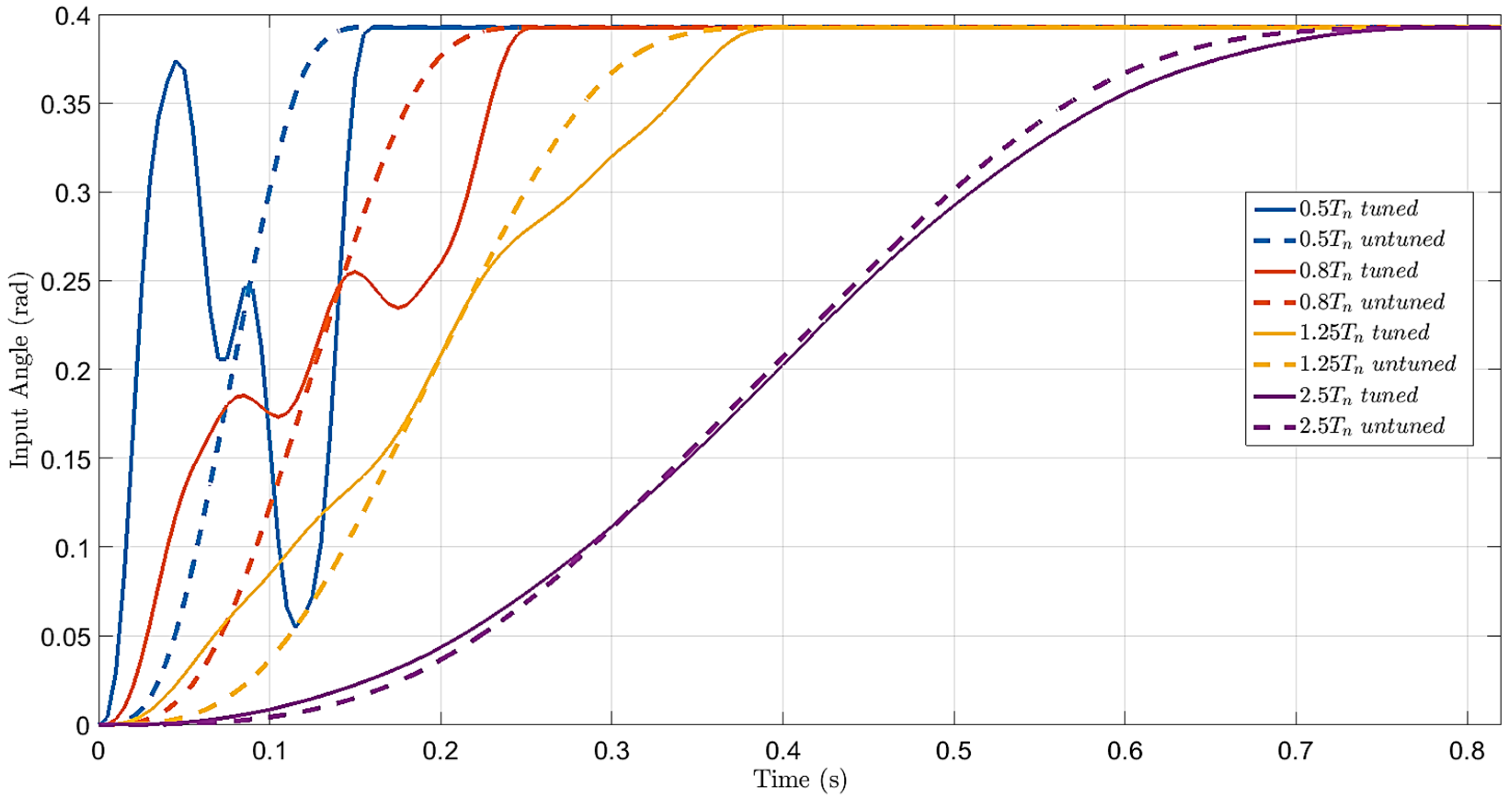
For the untuned command, the amplitudes $A_1,$ $A_2$, and $A_3$ were arbitrarily set to A/3, and the complete profile was constructed using Equations (16)–(19). In contrast, the tuned acceleration profile was obtained by first determining the parameters from Equations (13) and (15), and then generating the complete motion using Equations (16)–(19). Figure 10 shows the input angle profiles for the tuned and untuned motions with motion durations equal to ${0.5\tau }_n$, ${0.8\tau }_n$, ${1.25\tau }_n$, and ${2.5\tau }_n$. The corresponding simulation and experimental responses for the underdamped link (Link 2) at the selected motion durations are presented in Figure 11, Figure 12, Figure 13 and Figure 14.

Figure 10. Input angle profiles used for the tuned and untuned motions of the underdamped flexible beam.

Figure 11. Simulation and experimental results of tuned and untuned signals for Link 2 at $\mathit{T}=\mathbf{0.5}{\mathit{\tau }}_{\mathit{n}}.$

Figure 12. Simulation and experimental results of tuned and untuned signals for Link 2 at $\mathit{T}=\mathbf{0.8}{\mathit{\tau }}_{\mathit{n}}.$

Figure 13. Simulation and experimental results of tuned and untuned signals for Link 2 at $\mathit{T}=\mathbf{1.25}{\mathit{\tau }}_{\mathit{n}}.$

Figure 14. Simulation and experimental results of tuned and untuned signals for Link 2 at $\mathit{T}=\mathbf{2.5}{\mathit{\tau }}_{\mathit{n}}.$

As shown in Figure 11 and Figure 12, higher-frequency oscillatory components become more noticeable when the motion duration is shorter than one first-mode natural period. Based on the experimentally identified modal frequencies, these components are consistent with contributions from the second vibration mode. In contrast, as shown in Figure 13 and Figure 14, the higher-frequency components become considerably less noticeable for motion durations longer than one first-mode natural period, and the measured response is predominantly governed by the first mode. The tabulated form of the maximum residual vibration amplitudes at the endpoint of the underdamped flexible link after the tuned and untuned commands ended are given in Table 3.

Table 3. Maximum Residual Vibration Amplitudes measured at the tip of Flexible Link 2.

Total Travel Time	Simulation (mm)			Experimental (mm)
	Untuned	Tuned	Reduction (%)	Untuned	Tuned	Reduction (%)
0.5 ${\tau }_n$	106.70	2.50	97.66	112.60	12.10 *	NA *
0.8 ${\tau }_n$	83.51	0.08	99.90	89.45	4.00	95.53
1.25 ${\tau }_n$	36.40	0.00	100	37.00	1.80	95.14
2.5 ${\tau }_n$	4.50	0.00	100	5.00	0.40	92

* When higher-order vibration modes are excited, the tip displacement may not fully represent the overall vibration level of the flexible link [24]. At T = 0.5τ_n, the contribution of the second vibration mode becomes appreciable. The tip-mounted IMU therefore measures the combined local rotation associated with the first and second modes, whereas the angle-to-displacement conversion is based on the dominant first-mode relationship. Consequently, the corresponding experimental reduction value is reported as NA.

The simulation and experimental results show a consistent overall trend of substantial residual-vibration suppression. However, exact quantitative agreement is not obtained in all cases, particularly for the shorter tuned motions of the underdamped link. For T = 0.8τ_n, 1.25τ_n, and 2.5τ_n, the absolute differences between the simulated and experimental tuned residual-vibration amplitudes are 3.92, 1.80, and 0.40 mm, respectively. The numerical model applies the prescribed acceleration directly and retains only the dominant first vibration mode; therefore, second mode contributions do not appear in the simulated response. Such contributions may become more noticeable in the physical system, particularly during short motions. In addition, the numerical model does not include the dynamics of the servo drive and controller, command-tracking errors, gearbox effects, nonlinearities present in the experimental system.

7. Sensitivity to Parameter Mismatch and Comparison with ZV Input Shaping

For comparison with conventional ZV input shaping, the ZV-shaped command was generated using an acceleration-based template because the proposed method is formulated directly at the acceleration-command level. This places both approaches in the same command domain and provides a consistent basis for evaluating their residual-vibration characteristics. The unshaped template was constructed using the same general acceleration-profile structure with equal component amplitudes, ${A_1=A}_2=A_3=A/3$, while vibration suppression was provided by the ZV shaper.

Let $T$ denote the prescribed total motion time and $t_2$ the application time of the second ZV impulse. Since convolution with the ZV shaper extends the original template by $t_2$, the duration of the unshaped template was selected as $T-t_2$. Consequently, the resulting ZV-shaped command and the proposed command both complete the prescribed displacement at the same total motion time $T$. The same system parameters and initial conditions were used in the simulations.

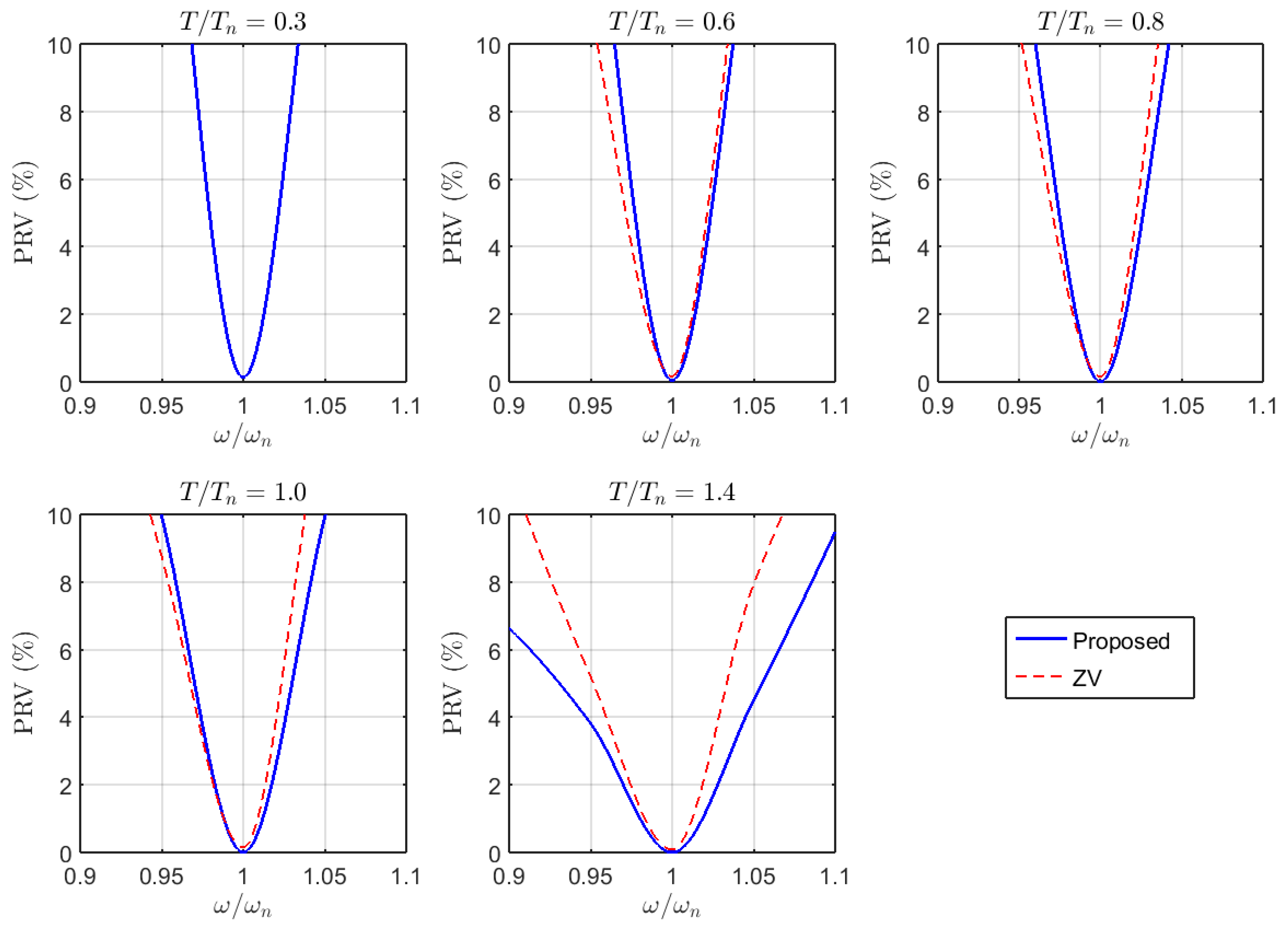
The sensitivity of the proposed and ZV-shaped profiles to errors in the parameters used for motion generation was examined at selected normalized motion times, $T/T_n$. Two types of parameter mismatch were considered: natural-frequency mismatch and damping-ratio mismatch. For the natural-frequency analysis, the frequency $w$ used to generate the motion command was varied while the actual natural frequency $w_n$ used in the governing differential equation was kept constant. For the damping-ratio analysis, the value $\zeta$ used for motion generation was varied while the actual system damping ratio ${\zeta }_{actual}$ was kept constant. The resulting PRV values were evaluated as functions of $w/w_n$ and $\zeta /{\zeta }_{actual}$, respectively. In both cases, a normalized parameter ratio of unity represents exact matching between the selected and actual system parameters.

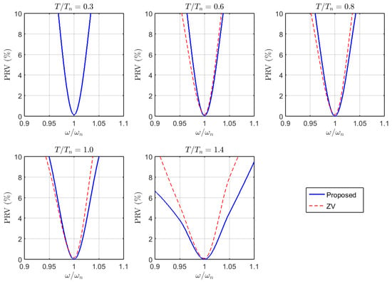
The natural-frequency sensitivity results obtained at selected normalized motion times are presented in Figure 15. In all cases, the PRV becomes zero at $w/w_n=$ 1, where the frequency selected for command generation matches the actual natural frequency of the system. At $T/T_n=$ 0.3, only the proposed profile is shown because this motion time is below the theoretical lower limit imposed by the second impulse of the underdamped ZV shaper under the equal-total-motion-time condition. At $T/T_n=$ 0.6, the ZV-shaped profile exhibits a somewhat wider low-PRV region than the proposed profile. At $T/T_n=$ 0.8 and 1, the sensitivity curves of the two methods are closely comparable. At $T/T_n=$ 1.4, however, the proposed profile maintains lower PRV values over a wider range of frequency-selection errors. The curves also become increasingly asymmetric about $w/w_n=$ 1, indicating that underestimation and overestimation of the natural frequency do not necessarily produce identical residual-vibration responses.

Figure 15. Sensitivity of PRV to natural-frequency mismatch for the proposed and ZV-shaped profiles at different normalized motion times.

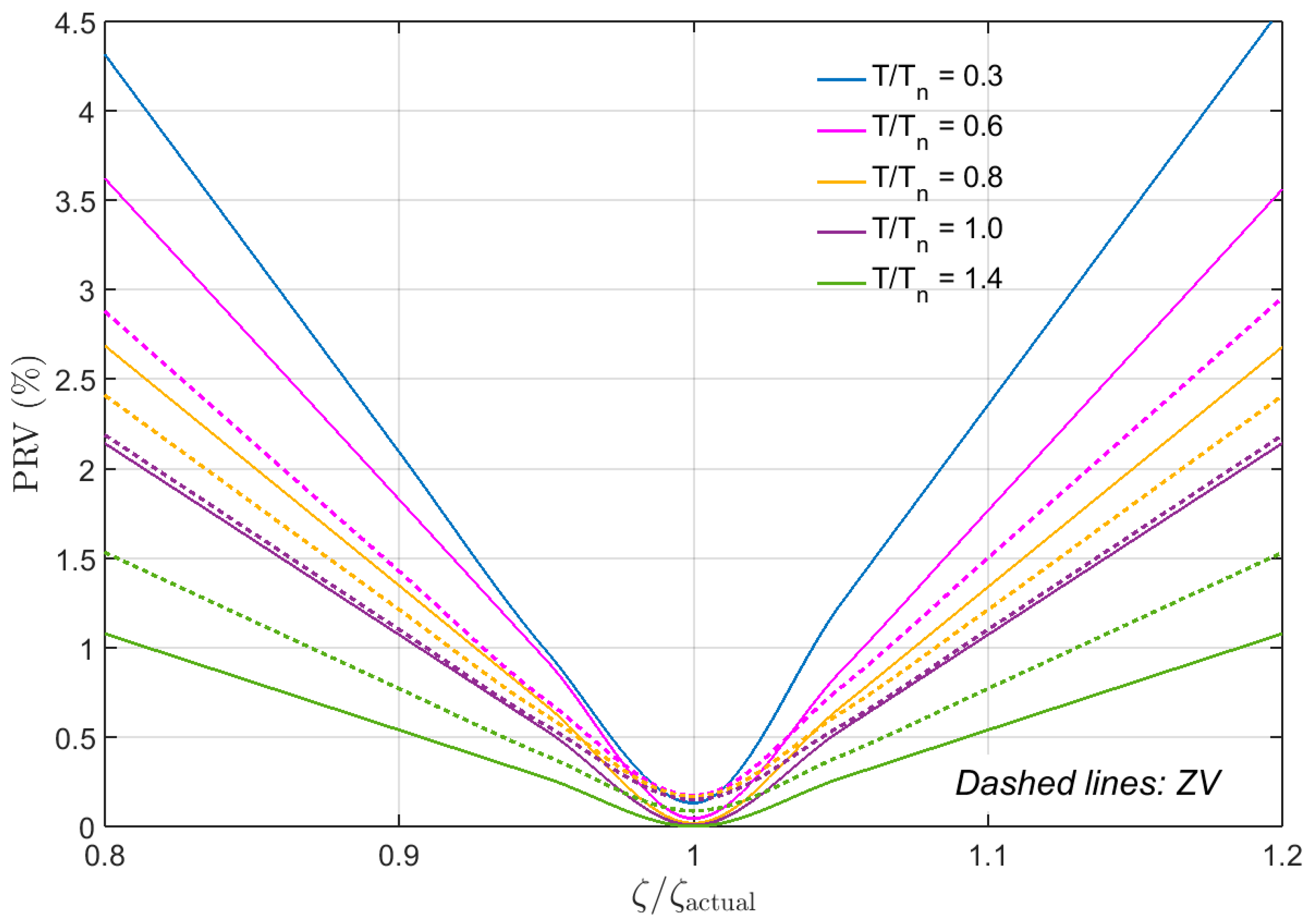
The damping-ratio sensitivity results are presented in Figure 16. The damping ratio $\zeta$ used for command generation was varied from 0.8 ${\zeta }_{actual}$ to 1.2 ${\zeta }_{actual}$, while the actual damping ratio used in the system model was kept constant. Thus, ${\displaystyle \frac{\zeta }{{\zeta }_{actual}}}=$ 1 represents exact matching, whereas values below and above unity correspond to underestimation and overestimation, respectively.

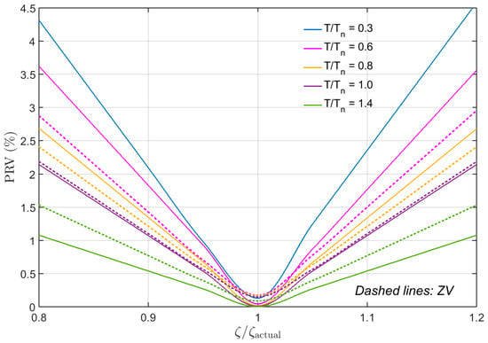
Figure 16. Sensitivity of PRV to damping ratio mismatch for the proposed and ZV-shaped profiles at different normalized motion times (solid lines: proposed; dashed lines: ZV).

For both methods, the PRV reaches its minimum at $\zeta /{\zeta }_{actual}=$ 1. At $T/T_n=$ 0.3, only the proposed profile is shown because the ZV-shaped command is not applicable under the equal-total-motion-time condition. At $T/T_n=$ 0.6 and 0.8, the ZV-shaped profile produces slightly lower PRV values than the proposed profile over most of the examined mismatch range. The responses become nearly identical at $T/T_n=$ 1, whereas the proposed profile exhibits lower sensitivity at $T/T_n =$ 1.4. For both methods, the PRV remains below 5% throughout the investigated damping-ratio range, indicating relatively low sensitivity to the considered ±20% damping-ratio mismatch.

8. Conclusions

This study presented a motion tuning approach for reducing residual vibrations in flexible link manipulators. The method is based on a four-segment acceleration profile formed by combining ramp, cycloidal, and ramped-versine functions. Within the scope of the reference motion profiles examined in this study, the proposed approach allows the motion duration to be specified without imposing an integer- or half-integer-period condition for residual-vibration suppression. Removing this restriction allows the motion time to be selected according to practical or process requirements rather than the natural period of the system. This is particularly useful in high-speed positioning applications where the available motion time may be limited.

The proposed method was evaluated through numerical simulations and experiments using flexible links with different damping characteristics. The results showed that residual vibration can be substantially reduced over a wide range of travel times. Effective suppression was also obtained for motions completed in less than one natural period.

The main findings of this study are as follows:

• The proposed motion profile substantially reduced residual vibration over the range of travel times considered, including motions shorter than one natural period.
• The simulation and experimental results showed a consistent overall trend of substantial residual-vibration suppression, although quantitative differences remained, particularly for the shorter tuned motions of the underdamped link.
• Increasing the motion duration beyond a certain point produced only a small additional reduction in residual vibration. Therefore, using longer motion times may not provide a practical advantage when vibration has already been reduced to a sufficiently low level.
• When the motion duration was shorter than one natural period, higher vibration modes became more noticeable in the experimental response. However, their amplitudes remained relatively small, while the dominant first-mode vibration was effectively suppressed.
• Quantitatively, the reduction in dominant first-mode residual-vibration amplitude ranged from 97.24% to 100% in the simulations and from 92% to 98% in the experiments for the cases included in the comparison, relative to the corresponding untuned commands.

Overall, the proposed method offers a direct way of designing motion profiles for flexible systems. The acceleration profile itself is tuned according to the system dynamics, so vibration suppression is incorporated at the motion-design stage rather than through modification of a predefined motion command. This provides flexibility in selecting the motion duration according to the requirements of the application.

The present method has some limitations that define the scope of the results. The formulation is based on the dominant first vibration mode and does not explicitly impose suppression conditions on higher modes. In addition, the tuning relies on the identified modal parameters of the flexible system. The method does not impose a theoretical lower bound on the motion duration relative to the natural period; however, shorter motion durations require increased acceleration and jerk levels. Therefore, the practically achievable motion duration depends on the physical capabilities of the particular system in which the tuned motion profile is implemented. Extension to multimode systems and further investigation of parameter sensitivity constitute directions for future work.

References

- Alhazza, K. A multi-mode analytical frequency modulation input-shaping control. Int. J. Mech. Syst. Dyn. 2025, 5, 415–425. [Google Scholar] [CrossRef] [Scilit]
- Fang, Y.; Zhu, G.-N.; Zhao, Y.; Gu, C. Design procedure for motion profiles with sinusoidal jerk for vibration reduction. Appl. Sci. 2023, 13, 13320. [Google Scholar] [CrossRef] [Scilit]
- Cui, X.; Fang, Y.; Gu, C. Residual vibration reduction in flexible systems based on trapezoidal velocity profiles. Appl. Sci. 2025, 15, 1791. [Google Scholar] [CrossRef] [Scilit]
- Mohamed, Z.; Tokhi, M.O. Command shaping techniques for vibration control of a flexible robot manipulator. Mechatronics 2004, 14, 69–90. [Google Scholar] [CrossRef] [Scilit]
- Cuccio, A.; Garziera, R.; Righettini, P. Vibration control input-laws in point-to-point motion: Theory and experiments. Mech. Mach. Theory 1998, 33, 341–349. [Google Scholar] [CrossRef] [Scilit]
- Aspinwall, D.M. Acceleration profiles for minimizing residual response. J. Dyn. Syst. Meas. Control 1980, 102, 3–6. [Google Scholar] [CrossRef] [Scilit]
- Meckl, P.H.; Seering, W.P. Controlling velocity-limited systems to reduce residual vibration. In Proceedings of the IEEE International Conference on Robotics and Automation; IEEE: New York, NY, USA, 1988; pp. 1428–1433. [Google Scholar] [CrossRef] [Scilit]
- Liu, Y.; Cheng, L. Generalized adaptive delayed resonator design for complete vibration suppression with force-tuning inaccuracies. IEEE Trans. Ind. Electron. 2025, 73, 6242–6253. [Google Scholar] [CrossRef] [Scilit]
- Alnefaie, K.; Diken, H.; Alghamdi, A. Residual vibration of a rotating flexible beam subject to prescribed motion. J. King Abdulaziz Univ. Eng. Sci. 2009, 20, 97–107. [Google Scholar] [CrossRef] [Scilit]
- Shin, K.; Brennan, M.J. Two simple methods to suppress the residual vibrations of a translating or rotating flexible cantilever beam. J. Sound Vib. 2008, 312, 140–150. [Google Scholar] [CrossRef] [Scilit]
- Önsay, T.; Akay, A. Vibration reduction of a flexible arm by time-optimal open-loop control. J. Sound Vib. 1991, 147, 283–300. [Google Scholar] [CrossRef] [Scilit]
- Singer, N.C.; Seering, W.P. Preshaping command inputs to reduce system vibration. J. Dyn. Syst. Meas. Control 1990, 112, 76–82. [Google Scholar] [CrossRef] [Scilit]
- Singer, N.C. Residual Vibration Reduction in Computer-Controlled Machines. Ph.D. Thesis, Massachusetts Institute of Technology, Cambridge, MA, USA, 1988. Available online: https://dspace.mit.edu/handle/1721.1/14435 (accessed on 20 September 2026).
- Kapucu, S.; Alici, G.; Baysec, S. Residual swing/vibration reduction using a hybrid input shaping method. Mech. Mach. Theory 2001, 36, 311–326. [Google Scholar] [CrossRef] [Scilit]
- Yavuz, H.; Mıstıkoğlu, S.; Kapucu, S. Hybrid input shaping to suppress residual vibration of flexible systems. J. Vib. Control 2011, 18, 132–140. [Google Scholar] [CrossRef] [Scilit]
- Alici, G.; Kapucu, S.; Baysec, S. A robust motion design technique for flexible-jointed manipulation systems. Robotica 2006, 24, 95–103. [Google Scholar] [CrossRef] [Scilit]
- Meckl, P.H.; Arestides, P.B. Optimized S-curve motion profiles for minimum residual vibration. In Proceedings of the American Control Conference; IEEE: New York, NY, USA, 1998; pp. 2627–2631. [Google Scholar] [CrossRef] [Scilit]
- Li, H.; Le, M.D.; Gong, Z.M.; Lin, W. Motion profile design to reduce residual vibration of high-speed positioning stages. IEEE/ASME Trans. Mechatron. 2009, 14, 264–269. [Google Scholar] [CrossRef] [Scilit]
- Ha, C.; Rew, K.; Kim, K. Robust zero placement for motion control of lightly damped systems. IEEE Trans. Ind. Electron. 2013, 60, 3857–3864. [Google Scholar] [CrossRef] [Scilit]
- Béarée, R.; Olabi, A. Dissociated jerk-limited trajectory applied to time-varying vibration reduction. Robot. Comput.-Integr. Manuf. 2013, 29, 444–453. [Google Scholar] [CrossRef] [Scilit]
- Kim, B.; Yoo, H.H.; Chung, J. Robust motion profiles for the residual vibration reduction of an undamped system. J. Mech. Sci. Technol. 2017, 31, 4647–4656. [Google Scholar] [CrossRef] [Scilit]
- Akdağ, M.; Şen, H. S-curve motion profile design for vibration control of single link flexible manipulator. Dokuz Eylül Üniversitesi Mühendis. Fakültesi Fen Mühendis. Derg. 2021, 23, 661–676. [Google Scholar] [CrossRef] [Scilit]
- Yavuz, Ş.; Malgaca, L.; Karagülle, H. Vibration control of a single-link flexible composite manipulator. Compos. Struct. 2016, 140, 684–691. [Google Scholar] [CrossRef] [Scilit]
- Alawadhi, A.M.; Alabdullah, M.A.; Alhazza, K.A. Single-mode input shaping for multi-mode vibration suppression in flexible robotic manipulators: An experimental validation of mode alignment via mass addition. Int. J. Dyn. Control 2025, 13, 171. [Google Scholar] [CrossRef] [Scilit]
- Shi, M.; Cheng, Y.; Rong, B.; Zhao, W.; Yao, Z.; Yu, C. Research on vibration suppression and trajectory tracking control strategy of a flexible link manipulator. Appl. Math. Model. 2022, 110, 78–98. [Google Scholar] [CrossRef] [Scilit]
- Boscariol, P.; Richiedei, D.; Tamellin, I. Residual vibration suppression in uncertain systems: A robust structural modification approach to trajectory planning. Robot. Comput.-Integr. Manuf. 2022, 74, 102282. [Google Scholar] [CrossRef] [Scilit]
- Kaya, F.; Conker, Ç. Design and multi-objective optimization of a novel robust command shaping technique for the tolerable level of residual vibration. Mechatronics 2026, 113, 103426. [Google Scholar] [CrossRef] [Scilit]
- Hastings, G.; Book, W. A linear dynamic model for flexible robotic manipulators. IEEE Control Syst. Mag. 1987, 7, 61–64. [Google Scholar] [CrossRef] [Scilit]
- Martins, J.M.; Mohamed, Z.; Tokhi, M.O.; Sa da Costa, J.; Botto, M.A. Approaches for dynamic modelling of flexible manipulator systems. IEE Proc.-Control Theory Appl. 2003, 150, 401–411. [Google Scholar] [CrossRef] [Scilit]
- Clough, R.W.; Penzien, J. Dynamics of Structures; McGraw-Hill: New York, NY, USA, 1975. [Google Scholar]
- Erturk, A.; Inman, D.J. Piezoelectric Energy Harvesting; Wiley: Chichester, UK, 2011. [Google Scholar]
- Kim, D.W.; Kwak, M.K.; Kim, S.-M.; Feeny, B.F. Slewing and active vibration control of a flexible single-link manipulator. Actuators 2025, 14, 43. [Google Scholar] [CrossRef] [Scilit]
- Sakawa, Y.; Matsuno, F.; Fukushima, S. Modeling and feedback control of a flexible arm. J. Robot. Syst. 1985, 2, 453–472. [Google Scholar] [CrossRef] [Scilit]
- Masoud, Z.N.; Alhazza, K.A.; Nazzal, M.A. Multimode input shaping control of flexible structures using frequency modulation. In Proceedings of the ASME International Design Engineering Technical Conferences and Computers and Information in Engineering Conference; Paper No. DETC2016-59537; ASME: New York, NY, USA, 2016. [Google Scholar] [CrossRef] [Scilit]
- Stretti, D.; Fanghella, P.; Berselli, G.; Bruzzone, L. Analytical expression of motion profiles with elliptic jerk. Robotica 2023, 41, 1976–1990. [Google Scholar] [CrossRef] [Scilit]
- Alici, G.; Kapucu, S.; Baysec, S. Swing-free transportation of suspended objects with robot manipulators. Robotica 1999, 17, 513–521. [Google Scholar] [CrossRef] [Scilit]
- Conker, Ç.; Yavuz, H.; Kapucu, S.; Baltacıoğlu, M.K.; Arat, H.T.; Burgaç, A. Comparison of robust input shapers for elimination of residual vibrations. Appl. Mech. Mater. 2014, 490–491, 997–1002. [Google Scholar] [CrossRef] [Scilit]
- Conker, Ç.; Yavuz, H.; Bilgiç, H.H. A review of command shaping techniques for elimination of residual vibrations in flexible-joint manipulators. J. Vibroeng. 2016, 18, 2947–2958. [Google Scholar] [CrossRef] [Scilit]
- Delta. Products—Servo Systems—AC Servo Motors and Drives. Available online: https://www.deltaww.com/en-US/products/Servo-Systems-AC-Servo-Motors-and-Drives/23 (accessed on 10 August 2026).
- Movella. Xsens MTw Awinda. Available online: https://www.movella.com/products/wearables/xsens-mtw-awinda (accessed on 10 August 2026).
- Kozak, K.; Huey, J.; Singhose, W. Performance measures for input shaping. In Proceedings of the IEEE Conference on Control Applications; IEEE: New York, NY, USA, 2003; pp. 1227–1232. [Google Scholar] [CrossRef] [Scilit]
- Ankarali, A.; Diken, H. Vibration control of an elastic manipulator link. J. Sound Vib. 1997, 204, 162–170. [Google Scholar] [CrossRef] [Scilit]
Disclaimer/Publisher’s Note: The statements, opinions and data contained in all publications are solely those of the individual author(s) and contributor(s) and not of MDPI and/or the editor(s). MDPI and/or the editor(s) disclaim responsibility for any injury to people or property resulting from any ideas, methods, instructions or products referred to in the content. |
© 2026 by the authors. Licensee MDPI, Basel, Switzerland. This article is an open access article distributed under the terms and conditions of the Creative Commons Attribution (CC BY) license.