


Abstract
The theory of generalized locally Toeplitz (GLT) sequences is a powerful apparatus for computing the asymptotic spectral distribution of matrices arising from virtually any kind of numerical discretization of differential equations (DEs). Indeed, when the mesh fineness parameter n tends to infinity, these matrices give rise to a sequence , which often turns out to be a GLT sequence or one of its “relatives”, i.e., a block GLT sequence or a reduced GLT sequence. In particular, block GLT sequences are encountered in the discretization of systems of DEs as well as in the higher-order finite element or discontinuous Galerkin approximation of scalar DEs. Despite the applicative interest, a solid theory of block GLT sequences has been developed only recently, in 2018. The purpose of the present paper is to illustrate the potential of this theory by presenting a few noteworthy examples of applications in the context of DE discretizations.
Keywords:
spectral (eigenvalue) and singular value distributions; generalized locally Toeplitz sequences; discretization of systems of differential equations; higher-order finite element methods; discontinuous Galerkin methods; finite difference methods; isogeometric analysis; B-splines; curl–curl operator; time harmonic Maxwell’s equations and magnetostatic problems MSC:
47B06; 15A18; 15B05; 65N30; 65N06; 65D07
1. Introduction
The theory of generalized locally Toeplitz (GLT) sequences stems from Tilli’s work on locally Toeplitz (LT) sequences [1] and from the spectral theory of Toeplitz matrices [2,3,4,5,6,7,8,9,10,11,12]. It was then carried forward in [13,14,15,16], and was recently extended by Barbarino [17]. This theory is a powerful apparatus for computing the asymptotic spectral distribution of matrices arising from the numerical discretization of continuous problems, such as integral equations (IEs) and, especially, differential equations (DEs). The experience reveals that virtually any kind of numerical methods for the discretization of DEs gives rise to structured matrices whose asymptotic spectral distribution, as the mesh fineness parameter n tends to infinity, can be computed through the theory of GLT sequences. We refer the reader to ([13] Section 10.5), ([14] Section 7.3), and [15,16,18] for applications of the theory of GLT sequences in the context of finite difference (FD) discretizations of DEs; to ([13] Section 10.6), ([14] Section 7.4), and [16,18,19] for the finite element (FE) case; to [20] for the finite volume (FV) case; to ([13] Section 10.7), ([14] Sections 7.5–7.7), and [21,22,23,24,25,26] for the case of isogeometric analysis (IgA) discretizations, both in the collocation and Galerkin frameworks; and to [27] for a further recent application to fractional DEs. We also refer the reader to ([13] Section 10.4) and [28,29] for a look at the GLT approach for sequences of matrices arising from IE discretizations.
It is worth emphasizing that the asymptotic spectral distribution of DE discretization matrices, whose computation is the main objective of the theory of GLT sequences, is not only interesting from a theoretical viewpoint, but can also be used for practical purposes. For example, it is known that the convergence properties of mainstream iterative solvers, such as multigrid and preconditioned Krylov methods, strongly depend on the spectral features of the matrices to which they are applied. The spectral distribution can then be exploited to design efficient solvers of this kind and to analyze/predict their performance. In this regard, we recall that noteworthy estimates on the superlinear convergence of the conjugate gradient method obtained by Beckermann and Kuijlaars in [30] are closely related to the asymptotic spectral distribution of the considered matrices. Furthermore, in the context of Galerkin and collocation IgA discretizations of elliptic DEs, the spectral distribution computed through the theory of GLT sequences in a series of recent papers [21,22,23,24,25] was exploited in [31,32,33] to devise and analyze optimal and robust multigrid solvers for IgA linear systems.
In the very recent work [34], starting from the original intuition by the third author ([16] Section 3.3), the theory of block GLT sequences has been developed in a systematic way as an extension of the theory of GLT sequences. Such an extension is of the utmost importance in practical applications. In particular, it provides the necessary tools for computing the spectral distribution of block structured matrices arising from the discretization of systems of DEs ([16] Section 3.3) and from the higher-order finite element or discontinuous Galerkin approximation of scalar/vectorial DEs [35,36,37]. The purpose of this paper is to illustrate the potential of the theory of block GLT sequences [34] and of its multivariate version—which combines the results of [34] with the “multivariate technicalities” from [14]—by presenting a few noteworthy examples of applications. Actually, the present paper can be seen as a necessary completion of the purely theoretical work [34].
The paper is organized as follows. In Section 2, we report a summary of the theory of block GLT sequences. In Section 3, we focus on the FD discretization of a model system of univariate DEs; through the theory of block GLT sequences, we compute the spectral distribution of the related discretization matrices. In Section 4, we focus on the higher-order FE approximation of the univariate diffusion equation; again, we compute the spectral distribution of the associated discretization matrices through the theory of block GLT sequences. In Section 5, we summarize the multivariate version of the theory of block GLT sequences, also known as the theory of multilevel block GLT sequences. In Section 6, we describe the general GLT approach for computing the spectral distribution of matrices arising from the discretization of systems of partial differential equations (PDEs). In Section 7, we focus on the B-spline IgA approximation of a bivariate variational problem for the curl–curl operator, which is of interest in magnetostatics; through the theory of multilevel block GLT sequences, we compute the spectral distribution of the related discretization matrices. Final considerations are collected in Section 8.
2. The Theory of Block GLT Sequences
In this section, we summarize the theory of block GLT sequences, which was originally introduced in ([16] Section 3.3) and has been recently revised and systematically developed in [34].
Sequences of Matrices and Block Matrix-Sequences. Throughout this paper, a sequence of matrices is any sequence of the form , where is a square matrix of size and as . Let be a fixed positive integer independent of n; an s-block matrix-sequence (or simply a matrix-sequence if s can be inferred from the context or we do not need/want to specify it) is a special sequence of matrices in which the size of is .
Singular Value and Eigenvalue Distribution of a Sequence of Matrices. Let be the Lebesgue measure in . Throughout this paper, all the terminology from measure theory (such as “measurable set”, “measurable function”, “a.e.”, etc.) is referred to the Lebesgue measure. A matrix-valued function is said to be measurable (resp., continuous, Riemann-integrable, in , etc.) if its components , are measurable (resp., continuous, Riemann-integrable, in , etc.). We denote by (resp., ) the space of continuous complex-valued functions with bounded support defined on (resp., ). If , the singular values and the eigenvalues of A are denoted by and , respectively.
Definition 1.
Let be a sequence of matrices, with of size , and let be a measurable function defined on a set D with .
- We say that has a (asymptotic) singular value distribution described by f, and we write , ifIn this case, f is referred to as a singular value symbol of .
- We say that has a (asymptotic) spectral (or eigenvalue) distribution described by f, and we write , ifIn this case, f is referred to as a spectral (or eigenvalue) symbol of .
If has both a singular value and an eigenvalue distribution described by f, we write .
We note that Definition 1 is well-posed because the functions and are measurable ([34] Lemma 2.1). Whenever we write a relation such as or , it is understood that f is as in Definition 1; that is, f is a measurable function defined on a subset D of some with , and f takes values in for some .
Remark 1.
The informal meaning behind the spectral distribution (2) is the following: assuming that f possesses r Riemann-integrable eigenvalue functions , , the eigenvalues of , except possibly for outliers, can be subdivided into r different subsets of approximately the same cardinality; and, for n large enough, the eigenvalues belonging to the ith subset are approximately equal to the samples of the ith eigenvalue function over a uniform grid in the domain D. For instance, if , , and , then, assuming we have no outliers, the eigenvalues of are approximately equal to
for n large enough; similarly, if , , and , then, assuming we have no outliers, the eigenvalues of are approximately equal to
for n large enough; and so on for . A completely analogous meaning can also be given for the singular value distribution (1).
Remark 2.
Let and let be a measurable function possessing r real-valued Riemann-integrable eigenvalue functions , . Compute for each the uniform samples
sort them in non-decreasing order and put them in a vector . Let be the piecewise linear non-decreasing function that interpolates the samples over the nodes , i.e.,
Suppose converges in measure over to some function ϕ as (this is always the case in real-world applications). Then,
This result can be proved by adapting the argument used in ([13] solution of Exercise 3.1). The function ϕ is referred to as the canonical rearranged version of f. What is interesting about ϕ is that, by (3), if then , i.e., if f is a spectral symbol of then the same is true for ϕ. Moreover, ϕ is a univariate scalar function and hence it is much easier to handle than f. According to Remark 1, assuming that ϕ is Riemann-integrable, if we have (and hence also ), then, for n large enough, the eigenvalues of , with the possible exception of outliers, are approximately equal to the samples of ϕ over a uniform grid in .
The next two theorems are useful tools for computing the spectral distribution of sequences formed by Hermitian or perturbed Hermitian matrices. For the related proofs, we refer the reader to ([38] Theorem 4.3) and ([39] Theorem 1.1). In the following, the conjugate transpose of the matrix A is denoted by . If and , we denote by the Schatten p-norm of A, i.e., the p-norm of the vector . The Schatten ∞-norm is the largest singular value of A and coincides with the spectral norm . The Schatten 1-norm is the sum of the singular values of A and is often referred to as the trace-norm of A. The Schatten 2-norm coincides with the Frobenius norm of A. For more on Schatten p-norms, see [40].
Theorem 1.
Let be a sequence of matrices, with Hermitian of size , and let be a sequence such that , , and as . Then, if and only if .
Theorem 2.
Let and be sequences of matrices, with and of size . Assume that:
- the matrices are Hermitian and ;
- ;
then .
Block Toeplitz Matrices. Given a function in , its Fourier coefficients are denoted by
where the integrals are computed componentwise. The nth block Toeplitz matrix generated by f is defined as
It is not difficult to see that all the matrices are Hermitian when f is Hermitian a.e.
Block Diagonal Sampling Matrices. For and , we define the block diagonal sampling matrix as the diagonal matrix
Zero-Distributed Sequences. A sequence of matrices such that is referred to as a zero-distributed sequence. Note that, for any , is equivalent to (throughout this paper, and denote the zero matrix and the identity matrix, respectively). Proposition 1 provides an important characterization of zero-distributed sequences together with a useful sufficient condition for detecting such sequences. Throughout this paper, we use the natural convention .
Proposition 1.
Let be a sequence of matrices, with of size .
- is zero-distributed if and only if with and .
- is zero-distributed if there exists a such that .
Approximating Classes of Sequences. The notion of approximating classes of sequences (a.c.s.) is the fundamental concept on which the theory of block GLT sequences is based.
Definition 2.
Let be a sequence of matrices, with of size , and let be a sequence of sequences of matrices, with of size . We say that is an approximating class of sequences (a.c.s.) for if the following condition is met: for every m there exists such that, for ,
where depend only on m and .
Roughly speaking, is an a.c.s. for if, for large m, the sequence approximates in the sense that is eventually equal to plus a small-rank matrix (with respect to the matrix size ) plus a small-norm matrix. It turns out that, for each fixed sequence of positive integers such that , the notion of a.c.s. is a notion of convergence in the space
More precisely, there exists a pseudometric in such that is an a.c.s. for if and only if as . We therefore use the convergence notation to indicate that is an a.c.s. for . A useful criterion to identify an a.c.s. is provided in the next proposition ([13] Corollary 5.3).
Proposition 2.
Let be a sequence of matrices, with of size , let be a sequence of sequences of matrices, with of size , and let . Suppose that for every m there exists such that, for ,
where . Then, .
If and are any two matrices, the tensor (Kronecker) product of X and Y is the matrix defined as follows:
We recall that the tensor product operation ⊗ is associative and bilinear. Moreover,
Finally, if can be multiplied and can be multiplied, then
Lemma 1.
For , let be a sequence of matrices and suppose that . Then,
Proof.
Let be the matrix having 1 in position and 0 elsewhere. Note that
Block GLT Sequences. Let be a fixed positive integer. An s-block GLT sequence (or simply a GLT sequence if s can be inferred from the context or we do not need/want to specify it) is a special s-block matrix-sequence equipped with a measurable function , the so-called symbol. We use the notation to indicate that is a GLT sequence with symbol . The symbol of a GLT sequence is unique in the sense that if and then a.e. in . The main properties of s-block GLT sequences proved in [34] are listed below. If A is a matrix, we denote by the Moore–Penrose pseudoinverse of A (recall that whenever A is invertible). If are measurable matrix-valued functions, we say that converges to f in measure (resp., a.e., in , etc.) if converges to in measure (resp., a.e., in , etc.) for all .
- GLT 1.
- If then . If, moreover, each is Hermitian, then .
- GLT 2.
- We have:
- if is in ;
- if is Riemann-integrable;
- if and only if .
- GLT 3.
- If and , then:
- ;
- for all ;
- ;
- provided that is invertible a.e.
- GLT 4.
- if and only if there exist s-block GLT sequences such that and in measure.
Remark 3.
The reader might be astonished by the fact that we have talked so far about block GLT sequences without defining them. Actually, we intentionally avoided giving a definition for two reasons. First, the definition is rather cumbersome as it requires introducing other related (and complicated) concepts such as “block LT operators” and “block LT sequences”. Second, from a practical viewpoint, the definition is completely useless because everything that can be derived from it can also be derived fromGLT 1–GLT 4(and in a much easier way). The reader who is interested in the formal definition of block GLT sequences can find it in ([34] Section 5) along with the proofs of properties GLT 1–GLT 4.
3. FD Discretization of a System of DEs
Consider the following system of DEs:
In this section, we consider the classical central FD discretization of (10). Through the theory of block GLT sequences, we show that the corresponding sequence of (normalized) FD discretization matrices enjoys a spectral distribution described by a matrix-valued function. We remark that the number 2, which identifies the matrix space where the spectral symbol takes values, coincides with the number of equations that compose the system (10). In what follows, we use the following notation:
The parameters may be either scalars or blocks for some , in which case the previous matrix is a block tridiagonal matrix.
3.1. FD Discretization
Let , and set and for . Using the classical central FD schemes and for the discretization of, respectively, the (negative) second derivative and the first derivative, for each we obtain the following approximations:
This means that the nodal values of the solutions of (10) satisfy approximately the equations
for . We then approximate the solution (resp., ) by the piecewise linear function that takes the value (resp., ) at for all , where and the vectors and solve the linear system
This linear system can be rewritten in matrix form as follows:
where ,
and
In view of (13), the linear system (12) is equivalent to
where , and
Let and be the components of and , respectively. When writing the linear system (11) in the form (14), we are implicitly assuming the following.
- The unknowns are sorted as follows:
- The equations are sorted as follows, in accordance with the ordering (16) for the unknowns:
Suppose we decide to change the ordering for both the unknowns and the equations. More precisely, suppose we opt for the following orderings.
- The unknowns are sorted as follows:
- The equations are sorted as follows, in accordance with the ordering (18) for the unknowns:
The matrix associated with the linear system (11) assuming the new orderings (18) and (19) is the block tridiagonal matrix given by
The matrix is similar to . Indeed, by permuting both rows and columns of according to the permutation we obtain . More precisely, let and be the vectors of the canonical basis of and , respectively, and let be the permutation matrix associated with the permutation , that is,
Then, .
3.2. GLT Analysis of the FD Discretization Matrices
The main result of this section (Theorem 3) shows that is a block GLT sequence whose spectral distribution is described by a matrix-valued symbol, which is obtained by replacing the matrix-sequences , , , appearing in the expression (15) of with the corresponding symbols , , , . In this regard, we note that, assuming for instance , we have
To prove (22), it suffices to observe that
where is the modulus of continuity of . Since as , it follows from Proposition 1 that , and so GLT 2 and GLT 3 immediately yield (22). The relations (23)–(25) are proved in the same way.
Theorem 3.
Suppose that . Then,
and
If, moreover, , then we also have
Proof.
From (20), we have
where is the matrix having 1 in position and 0 elsewhere. It is clear that, for every ,
as ; hence, by Proposition 1, GLT 2 and GLT 3,
Consequently, the decomposition (29), GLT 2 and GLT 3 imply (26), which in turn implies (27) by GLT 1. It only remains to prove (28) in the case where . In this case, we have
Consider the symmetric approximation of given by
It is not difficult to see that as by invoking the inequality
see, e.g., ([13] Section 2.4.1). Therefore:
- in view of the decomposition , we have by (26), Proposition 1, GLT 2 and GLT 3, so in particular by GLT 1 as is symmetric;
- as .
Thus, (28) follows from Theorem 2. ☐
Example 1.
Suppose that and , so that by Theorem 3. The eigenvalue functions of are given by
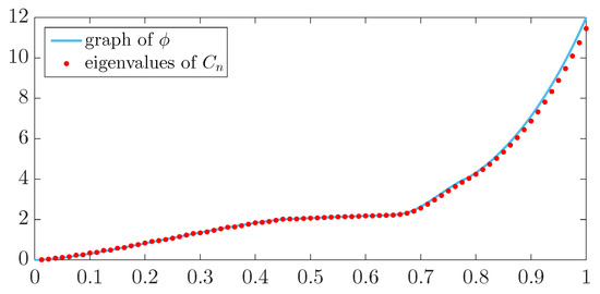
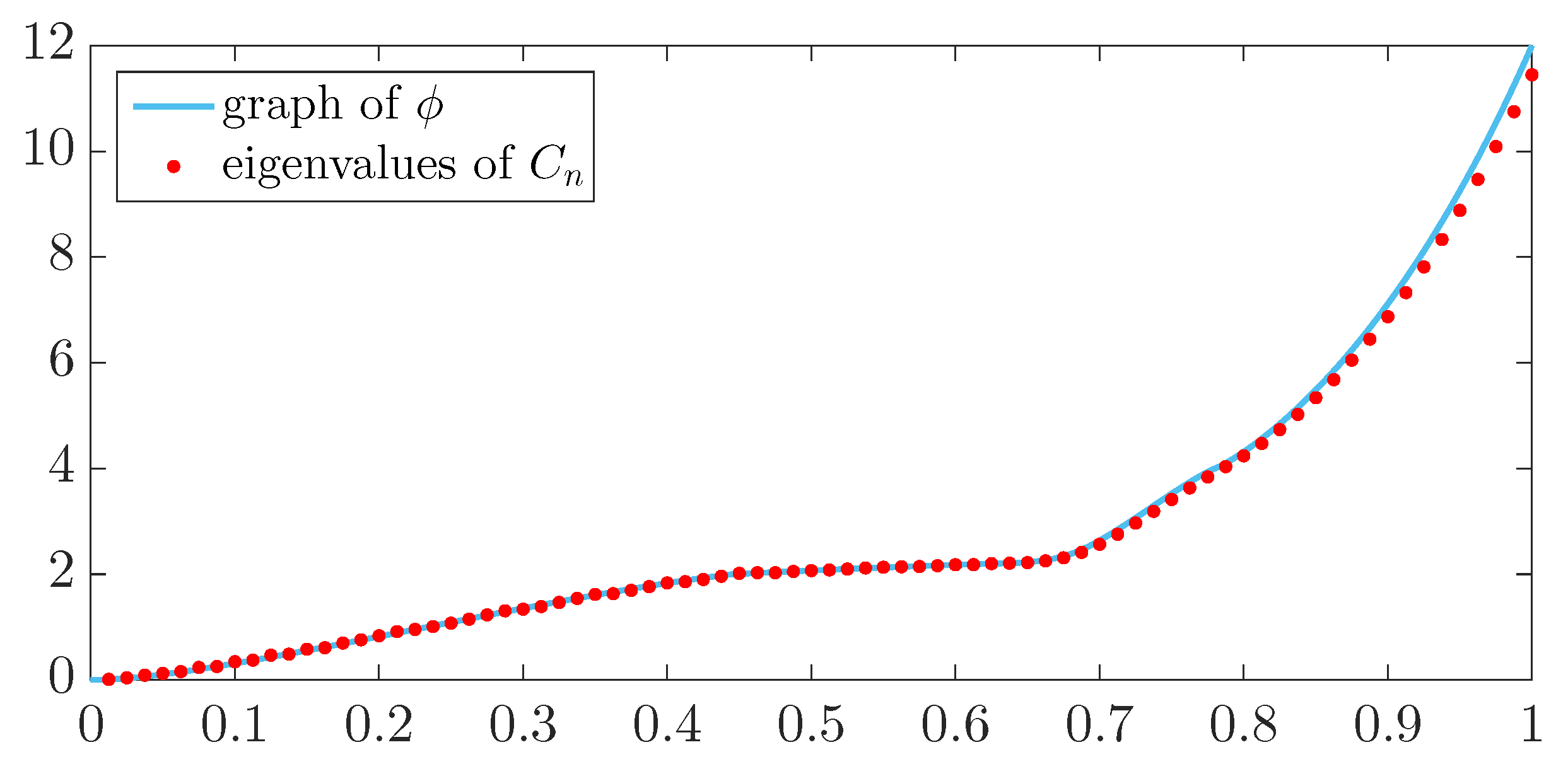
and are continuous on . Let ϕ be the canonical rearranged version of obtained as the limit of the piecewise linear functions , according to the construction in Remark 2. Figure 1 shows the graph of ϕ and the eigenvalues of for , , and . The graph of ϕ has been obtained by plotting the graph of corresponding to a large value of ρ. The eigenvalues of , which turn out to be real, although is not symmetric, have been sorted in non-decreasing order and placed at the points with , . We clearly see from the figure an excellent agreement between ϕ and the eigenvalues of , as predicted by Remark 2. In particular, we observe no outliers in this case.
Figure 1.
Comparison between the spectrum of and the rearranged version of the symbol for , , and .
4. Higher-Order FE Discretization of the Diffusion Equation
Consider the diffusion equation
In this section, we consider the higher-order FE discretization of (31). Through the theory of block GLT sequences, we show that the corresponding sequence of (normalized) FE discretization matrices enjoys a spectral distribution described by a matrix-valued function, where p and k represent, respectively, the degree and the smoothness of the piecewise polynomial functions involved in the FE approximation. Note that this result represents a remarkable argument in support of ([35] Conjecture 2).
4.1. FE Discretization
The weak form of (31) reads as follows: find such that
In the FE method, we fix a set of basis functions and we look for an approximation of the exact solution in the space by solving the following discrete problem: find such that
Since is a basis of , we can write for a unique vector . By linearity, the computation of (i.e., of ) reduces to solving the linear system
where and A is the stiffness matrix,
4.2. p-Degree B-spline Basis Functions
Following the higher-order FE approach, the basis functions will be chosen as piecewise polynomials of degree . More precisely, for and , let be the B-splines of degree p and smoothness defined on the knot sequence
We collect here a few properties of that we shall use in this paper. For the formal definition of B-splines, as well as for the proof of the properties listed below, see [41,42].
- The support of the ith B-spline is given by
- Except for the first and the last one, all the other B-splines vanish on the boundary of , i.e.,
- is a basis for the space of piecewise polynomial functions of degree p and smoothness , that is,where is the space of polynomials of degree . Moreover, is a basis for the space
- The B-splines form a non-negative partition of unity over :
- The derivatives of the B-splines satisfywhere is a constant depending only on p. Note that the derivatives may not be defined at some of the grid points in the case of smoothness (). In (38), it is assumed that the undefined values are excluded from the summation.
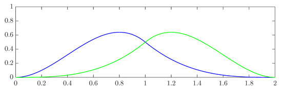
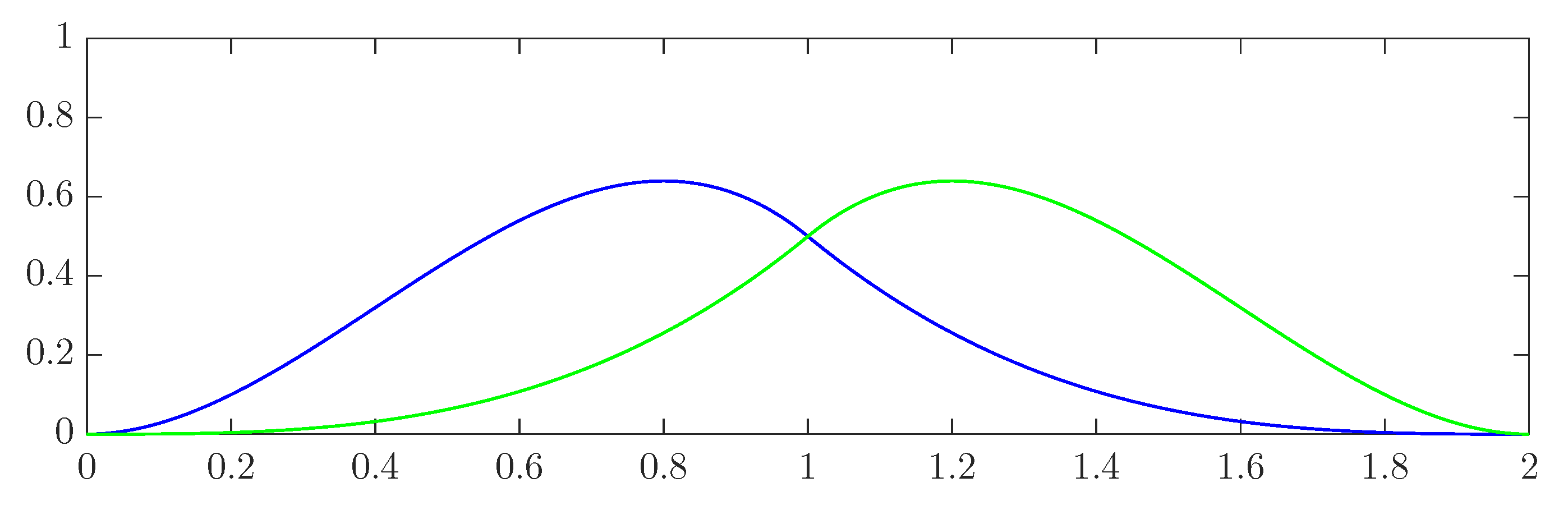
- All the B-splines, except for the first and the last , are uniformly shifted-scaled versions of fixed reference functions , namely the first B-splines defined on the reference knot sequence
Figure 2.
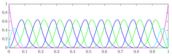
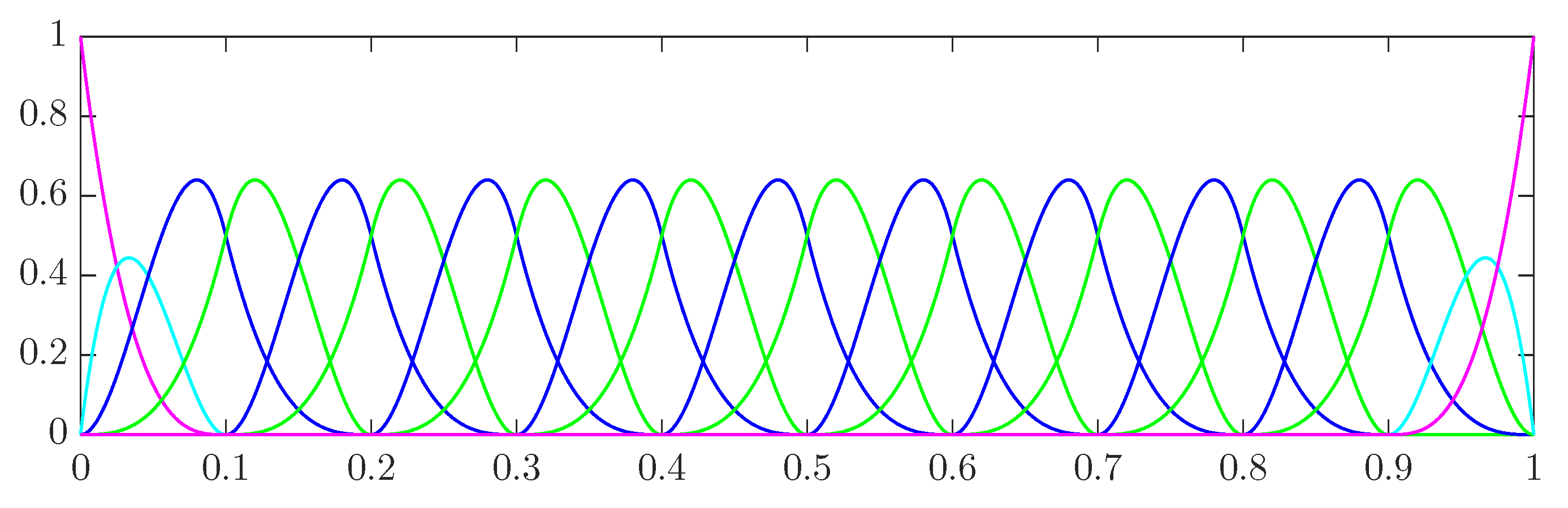
B-splines for and , with .
Figure 3.
Reference B-splines for and .
The basis functions are defined as follows:
In particular, with the notations of Section 4.1, we have and .
4.3. GLT Analysis of the Higher-Order FE Discretization Matrices
The stiffness matrix (32) resulting from the choice of the basis functions as in (41) will be denoted by ,
The main result of this section (Theorem 4) gives the spectral distribution of the normalized sequence . The proof of Theorem 4 is entirely based on the theory of block GLT sequences and it is therefore referred to as “GLT analysis”. It also requires the following lemma, which provides an approximate construction of the matrix corresponding to the constant-coefficient case where identically. In view of what follows, define the blocks
and the matrix-valued function ,
Due to the compact support of the reference functions , there is only a finite number of nonzero blocks and, consequently, the series in (44) is actually a finite sum.
Lemma 2.
Let and . Define as the principal submatrix of of size corresponding to the indices , where as in (39). Then, .
Theorem 4.
Let , and . Then, .
Proof.
The proof consists of four steps. Throughout this proof, we use the following notation.
- as in (39).
- For every square matrix A of size , we denote by the principal submatrix of A corresponding to the row and column indices .
- is the matrix having as the principal submatrix corresponding to the row and column indices and zeros elsewhere. Note that and for every square matrix A of size .
Step 1. Consider the linear operator ,
The next three steps are devoted to show that
Once this is done, the theorem is proven. Indeed, from (45), we immediately obtain the relation . We infer that by GLT 1 and by Theorem 1.
Step 2. We first prove (45) in the constant-coefficient case where identically. In this case, by Lemma 2, we have . Hence, the desired relation follows from GLT 2.
Step 3. Now we prove (45) in the case where . Let
By (33), (34) and (38), for all and , we have
where is the modulus of continuity of g and the last inequality is justified by the fact that the distance of the point from the interval is not larger than . It follows that each entry of is bounded in modulus by , where is a constant depending only on p. Moreover, by (34), the matrix is banded with bandwidth bounded by a constant depending only on p. Thus, by (30), as , and so is zero-distributed by Proposition 1. Since
we conclude that by GLT 2, GLT 3 and Step 2.
Step 4. Finally, we prove (45) in the general case where . By the density of in , there exist functions such that in . By Step 3,
Moreover,
We show that
Once this is done, the thesis (45) follows immediately from GLT 4. To prove (48), we recall that
see, e.g., ([13] Section 2.4.3). By (38), we obtain
Thus, the a.c.s. convergence (48) follows from Proposition 2. ☐
Remark 4.
By following step by step the proof of Theorem 4, we can give an alternative (much simpler) proof of ([36] Theorem A.6) based on the theory of block GLT sequences.
5. The Theory of Multilevel Block GLT Sequences
As illustrated in Section 3 and Section 4, the theory of block GLT sequences allows the computation of the singular value and eigenvalue distribution of block structured matrices arising from the discretization of univariate DEs. In order to cope with multivariate DEs, i.e., PDEs, we need the multivariate version of the theory of block GLT sequences, also known as the theory of multilevel block GLT sequences. The present section is devoted to a careful presentation of this theory, which is obtained by combining the results of [34] with the necessary technicalities for tackling multidimensional problems [14].
Multi-Index Notation. The multi-index notation is an essential tool for dealing with sequences of matrices arising from the discretization of PDEs. A multi-index , also called a d-index, is simply a (row) vector in ; its components are denoted by .
- are the vectors of all zeros, all ones, all twos, etc. (their size will be clear from the context).
- For any d-index , we set and we write to indicate that .
- If are d-indices, means that for all .
- If are d-indices such that , the multi-index range is the set . We assume for this set the standard lexicographic ordering:For instance, in the case , the ordering is the following: , , , , , , , , .
- When a d-index varies over a multi-index range (this is sometimes written as ), it is understood that varies from to following the specific ordering (50). For instance, if and if we write , then is a vector of size whose components , are ordered in accordance with (50): the first component is , the second component is , and so on until the last component, which is . Similarly, if , then X is a matrix whose components are indexed by two d-indices , both varying from to according to the lexicographic ordering (50).
- Given with , the notation indicates the summation over all in .
- Operations involving d-indices that have no meaning in the vector space must be interpreted in the componentwise sense. For instance, , etc.
Multilevel Block Matrix-Sequences. Given , a d-level s-block matrix-sequence (or simply a matrix-sequence if d and s can be inferred from the context or we do not need/want to specify them) is a sequence of matrices of the form , where:
- n varies in some infinite subset of ;
- is a d-index in which depends on n and satisfies as ;
- An is a square matrix of size .
Multilevel Block Toeplitz Matrices. Given a function in , its Fourier coefficients are denoted by
where and the integrals are computed componentwise. For , the nth multilevel block Toeplitz matrix generated by f is defined as
It is not difficult to see that the map is linear. Moreover, it can be shown that
where the transpose conjugate function is defined by ; in particular, all the matrices are Hermitian whenever f is Hermitian a.e. We also recall that, if and belong to , then
where is defined by ; see, e.g., ([14] Lemma 3.3).
Multilevel Block Diagonal Sampling Matrices. For and , we define the multilevel block diagonal sampling matrix as the block diagonal matrix
Multilevel Block GLT Sequences. Let be fixed positive integers. A d-level s-block GLT sequence (or simply a GLT sequence if d and s can be inferred from the context or we do not need/want to specify them) is a special d-level s-block matrix-sequence equipped with a measurable function , the so-called symbol. We use the notation to indicate that is a GLT sequence with symbol . The symbol of a GLT sequence is unique in the sense that if and then a.e. in . The main properties of d-level s-block GLT sequences are listed below.
- GLT 1.
- If then . If, moreover, each An is Hermitian then .
- GLT 2.
- We have:
- if is in ;
- if is Riemann-integrable;
- if and only if .
- GLT 3.
- If and then:
- ;
- for all ;
- ;
- provided that is invertible a.e.
- GLT 4.
- if and only if there exist GLT sequences such that and in measure.
6. Discretizations of Systems of PDEs: The General GLT Approach
In this section, we outline the main ideas of a multidimensional block GLT analysis for general discretizations of PDE systems. What we are going to present here is then a generalization of what is shown in Section 3. We begin by proving a series of auxiliary results. In the following, given and , we denote by the permutation matrix given by
where are the vectors of the canonical basis of , which, for convenience, are indexed by a d-index instead of a linear index . Note that coincides with the matrix in (21).
Lemma 3.
Let , let be in for , and set . The block matrix is similar via the permutation (53) to the multilevel block Toeplitz matrix , that is, .
Proof.
Let be the matrix having 1 in position and 0 elsewhere. Since and by the linearity of the map , it is enough to show that
Lemma 4.
Let , let for , and set . The block matrix is similar via the permutation (53) to the multilevel block diagonal sampling matrix , that is, .
Proof.
With obvious adaptations, it is the same as the proof of Lemma 3. ☐
We recall that a d-variate trigonometric polynomial is a finite linear combination of the d-variate Fourier frequencies .
Theorem 5.
For , let be a d-level 1-block GLT sequence with symbol . Set and . Then, the matrix-sequence is a d-level s-block GLT sequence with symbol κ.
Proof.
The proof consists of the following two steps.
Step 1. We first prove the theorem under the additional assumption that is of the form
where is Riemann-integrable, and belongs to . Note that the symbol of is
By setting and by adding zero matrices of the form in the summation (54) whenever , we can assume, without loss of generality, that
with L independent of . Let be the matrix having 1 in position and 0 elsewhere. Then,
By Lemmas 3 and 4,
It follows that
Thus, by GLT 2 and GLT 3, is a d-level s-block GLT sequence with symbol
Step 2. We now prove the theorem in its full generality. Since , by ([14] Theorem 5.6) there exist functions , such that
- and is a d-variate trigonometric polynomial,
- a.e.;
- .
Set and . We have:
- by Step 1;
- a.e. (and hence also in measure);
- because by Lemma 1.
We conclude that by GLT 4. ☐
Now, suppose we have a system of linear PDEs of the form
where . The matrices An resulting from any standard discretization of (55) are parameterized by a d-index , where is related to the discretization step in the ith direction, and if and only if (usually, ). By choosing each as a function of a unique discretization parameter , as it normally happens in practice where the most natural choice is for all , we see that and, consequently, is a (d-level) matrix-sequence. Moreover, it turns out that, after a suitable normalization that we ignore in this discussion—the normalization we are talking about is the analog of the normalization that we have seen in Section 3, which allowed us to pass from the matrix in (13) to the matrix in (15)—, An has the following block structure:
where is the (normalized) matrix arising from the discretization of the differential operator . In the simplest case where the operators have constant coefficients and we use equispaced grids in each direction, the matrix takes the form
where is a d-variate trigonometric polynomial, while the perturbation is usually a low-rank correction due to boundary conditions and, in any case, we have . Hence,
by GLT 2 and GLT 3, and it follows from Theorem 5 that
In the case where the operators have variable coefficients, the matrix usually takes the form
where is a d-variate trigonometric polynomial, , and the functions are related to the coefficients of (for example, in Section 3, while proving (22), we have seen that , which plays there the same role as the matrix here, is equal to for some zero-distributed sequence ). Hence,
by GLT 2 and GLT 3, and it follows from Theorem 5 that
7. B-Spline IgA Discretization of a Variational Problem for the Curl–Curl Operator
For any function , defined over some open set and taking values in , the curl operator is formally defined as follows:
Clearly, this definition has meaning when the components belong to , so that their partial derivatives exist in the Sobolev sense. Now, let , set
and consider the following variational problem: find such that
where is a vector field in and
Variational problems of the form of (56) arise in important applications, such as time harmonic Maxwell’s equations and magnetostatic problems. In this section, we consider a so-called compatible B-spline IgA discretization of (56); see [43] for details. We show that the corresponding sequence of discretization matrices enjoys a spectral distribution described by a matrix-valued function whose determinant is zero everywhere. The results of this section have already been obtained in [38], but the derivation presented here is entirely based on the theory of multilevel block GLT sequences and turns out to be simpler and more lucid than that in [38]. For simplicity, throughout this section, the B-splines , , and the associated reference B-spline , are denoted by , , and , respectively. The function is the so-called cardinal B-spline of degree p over the knot sequence . In view of the following, we recall from [42] and ([23] Lemma 4) that the cardinal B-spline is defined for all degrees , belongs to , and satisfies the following properties:
for ,
for and , and
for and . Moreover, property (40) in the case simplifies to
7.1. Compatible B-Spline IgA Discretization
Let , let , and define the space
Following a compatible B-spline approach [43], we look for an approximation of the solution in the space by solving the following discrete problem: find such that
After choosing a suitable ordering on the basis functions of displayed in (61), by linearity the computation of reduces to solving a linear system whose coefficient matrix is given by
where
Note that is a square matrix of size is a square matrix of size , while is a rectangular matrix of size .
7.2. GLT Analysis of the B-Spline IgA Discretization Matrices
In the main result of this section (Theorem 6), assuming that for a fixed vector , we show that the spectral distribution of the sequence is described by a matrix-valued function whose determinant is zero everywhere (Remark 5). To prove Theorem 6, some preliminary work is necessary. We first note that, in view of the application of Theorem 5, the matrix has an unpleasant feature: the anti-diagonal blocks and are not square and the square diagonal blocks and do not have the same size whenever . Let us then introduce the nicer matrix
where and are square matrices of size given by
Each block of the matrix is now a square block of size . Moreover,
where the matrix
satisfies . By (6) and (7),
and so
In view of the application of Theorem 1, we note that
Lemma 5.
Let and . Then,
where
and we note that the three series are actually finite sums because of (57).
Proof.
For every , since and , by (59) and (60) we obtain
Thus,
It follows from (72) that the principal submatrix of corresponding to the row and column indices is the zero matrix, which implies (66). Similarly, (73) and (74) imply (67) and (68), respectively. ☐
Theorem 6.
Let , let be a vector with positive components, and assume that (it is understood that n varies in the infinite subset of such that ). Then,
Proof.
The thesis follows immediately from Theorem 1 and (62)–(65) as soon as we have proven that
We show that
Once this is done, the thesis (75) follows immediately from Theorem 5 and GLT 1 as the matrix is symmetric. Actually, we only prove (76) for because the proof for the other pairs of indices is conceptually the same. Setting and keeping in mind the assumption , by Lemma 5 and Equations (5), (51) and (52), we have
where . Thus, by Proposition 1, and (76) (for ) follows from GLT 2 and GLT 3. ☐
Remark 5.
Using (58), it is not difficult to see that the functions and in (69) and (70) can be expressed in terms of as follows:
Therefore, the matrix-valued function appearing in Theorem 6 can be simplified as follows:
In particular, for all θ. According to the informal meaning behind the spectral distribution reported in Remark 1, this means that, for large n, one half of the eigenvalues of are approximately zero and one half is given by a uniform sampling over of
8. Conclusions
We have illustrated through specific examples the applicative interest of the theory of block GLT sequences and of its multivariate version, thus bringing to completion the purely theoretical work [34]. It should be said, however, that the theory of GLT sequences is still incomplete. In particular, besides filling in the details of the theory of multilevel block GLT sequences—the results of Section 5 have been obtained as a combination of the results in [14,34], but formal proofs of them are still missing and will be the subject of a future paper—, it will be necessary to develop the theory of the so-called reduced GLT sequences, as explained in ([13] Chapter 11).
Author Contributions
Funding
This research was funded by the Italian INdAM (Istituto Nazionale di Alta Matematica) through the grant PCOFUND-GA-2012-600198 and by the INdAM GNCS (Gruppo Nazionale per il Calcolo Scientifico) through a national grant.
Acknowledgments
C.G. is an INdAM Marie-Curie fellow under grant PCOFUND-GA-2012-600198. All authors are members of the INdAM GNCS, which partially supported this work.
Conflicts of Interest
The authors declare no conflict of interest.
References
- Tilli, P. Locally Toeplitz sequences: Spectral properties and applications. Linear Algebra Appl. 1998, 278, 91–120. [Google Scholar] [CrossRef] [Scilit]
- Avram, F. On bilinear forms in Gaussian random variables and Toeplitz matrices. Probab. Theory Relat. Fields 1988, 79, 37–45. [Google Scholar] [CrossRef] [Scilit]
- Böttcher, A.; Grudsky, S.M. Toeplitz Matrices, Asymptotic Linear Algebra, and Functional Analysis; Birkhäuser Verlag: Basel, Switzerland, 2000. [Google Scholar]
- Böttcher, A.; Grudsky, S.M. Spectral Properties of Banded Toeplitz Matrices; SIAM: Philadelphia, PA, USA, 2005. [Google Scholar]
- Böttcher, A.; Silbermann, B. Introduction to Large Truncated Toeplitz Matrices; Springer: New York, NY, USA, 1999. [Google Scholar]
- Böttcher, A.; Silbermann, B. Analysis of Toeplitz Operators, 2nd ed.; Springer: Berlin, Germany, 2006. [Google Scholar]
- Grenander, U.; Szego, G. Toeplitz Forms and Their Applications, 2nd ed.; AMS Chelsea Publishing: New York, NY, USA, 1984. [Google Scholar]
- Parter, S.V. On the distribution of the singular values of Toeplitz matrices. Linear Algebra Appl. 1986, 80, 115–130. [Google Scholar] [CrossRef] [Scilit]
- Tilli, P. A note on the spectral distribution of Toeplitz matrices. Linear Multilinear Algebra 1998, 45, 147–159. [Google Scholar] [CrossRef] [Scilit]
- Tyrtyshnikov, E.E. A unifying approach to some old and new theorems on distribution and clustering. Linear Algebra Appl. 1996, 232, 1–43. [Google Scholar] [CrossRef] [Scilit]
- Tyrtyshnikov, E.E.; Zamarashkin, N.L. Spectra of multilevel Toeplitz matrices: Advanced theory via simple matrix relationships. Linear Algebra Appl. 1998, 270, 15–27. [Google Scholar] [CrossRef]
- Zamarashkin, N.L.; Tyrtyshnikov, E.E. Distribution of eigenvalues and singular values of Toeplitz matrices under weakened conditions on the generating function. Sb. Math. 1997, 188, 1191–1201. [Google Scholar] [CrossRef] [Scilit]
- Garoni, C.; Serra-Capizzano, S. Generalized Locally Toeplitz Sequences: Theory and Applications, Volume I; Springer: Cham, Switzerland, 2017. [Google Scholar]
- Garoni, C.; Serra-Capizzano, S. Generalized Locally Toeplitz Sequences: Theory and Applications, Volume II; Springer; To appear.
- Serra-Capizzano, S. Generalized locally Toeplitz sequences: Spectral analysis and applications to discretized partial differential equations. Linear Algebra Appl. 2003, 366, 371–402. [Google Scholar] [CrossRef] [Scilit]
- Serra-Capizzano, S. The GLT class as a generalized Fourier analysis and applications. Linear Algebra Appl. 2006, 419, 180–233. [Google Scholar] [CrossRef] [Scilit]
- Barbarino, G. Equivalence between GLT sequences and measurable functions. Linear Algebra Appl. 2017, 529, 397–412. [Google Scholar] [CrossRef] [Scilit]
- Böttcher, A.; Garoni, C.; Serra-Capizzano, S. Exploration of Toeplitz-like matrices with unbounded symbols is not a purely academic journey. Sb. Math. 2017, 208, 1602–1627. [Google Scholar] [CrossRef] [Scilit]
- Beckermann, B.; Serra-Capizzano, S. On the asymptotic spectrum of finite element matrix sequences. SIAM J. Numer. Anal. 2007, 45, 746–769. [Google Scholar] [CrossRef] [Scilit]
- Bertaccini, D.; Donatelli, M.; Durastante, F.; Serra-Capizzano, S. Optimizing a multigrid Runge–Kutta smoother for variable-coefficient convection-diffusion equations. Linear Algebra Appl. 2017, 533, 507–535. [Google Scholar] [CrossRef] [Scilit]
- Donatelli, M.; Garoni, C.; Manni, C.; Serra-Capizzano, S.; Speleers, H. Spectral analysis and spectral symbol of matrices in isogeometric collocation methods. Math. Comput. 2016, 85, 1639–1680. [Google Scholar] [CrossRef] [Scilit]
- Garoni, C. Spectral distribution of PDE discretization matrices from isogeometric analysis: The case of L1 coefficients and non-regular geometry. J. Spectr. Theory 2018, 8, 297–313. [Google Scholar] [CrossRef] [Scilit]
- Garoni, C.; Manni, C.; Pelosi, F.; Serra-Capizzano, S.; Speleers, H. On the spectrum of stiffness matrices arising from isogeometric analysis. Numer. Math. 2014, 127, 751–799. [Google Scholar] [CrossRef] [Scilit]
- Garoni, C.; Manni, C.; Serra-Capizzano, S.; Sesana, D.; Speleers, H. Spectral analysis and spectral symbol of matrices in isogeometric Galerkin methods. Math. Comput. 2017, 86, 1343–1373. [Google Scholar] [CrossRef] [Scilit]
- Garoni, C.; Manni, C.; Serra-Capizzano, S.; Sesana, D.; Speleers, H. Lusin theorem, GLT sequences and matrix computations: An application to the spectral analysis of PDE discretization matrices. J. Math. Anal. Appl. 2017, 446, 365–382. [Google Scholar] [CrossRef] [Scilit]
- Roman, F.; Manni, C.; Speleers, H. Spectral analysis of matrices in Galerkin methods based on generalized B-splines with high smoothness. Numer. Math. 2017, 135, 169–216. [Google Scholar] [CrossRef] [Scilit]
- Donatelli, M.; Mazza, M.; Serra-Capizzano, S. Spectral analysis and structure preserving preconditioners for fractional diffusion equations. J. Comput. Phys. 2016, 307, 262–279. [Google Scholar] [CrossRef] [Scilit]
- Salinelli, E.; Serra-Capizzano, S.; Sesana, D. Eigenvalue–eigenvector structure of Schoenmakers–Coffey matrices via Toeplitz technology and applications. Linear Algebra Appl. 2016, 491, 138–160. [Google Scholar] [CrossRef] [Scilit]
- Al-Fhaid, A.S.; Serra-Capizzano, S.; Sesana, D.; Ullah, M.Z. Singular-value (and eigenvalue) distribution and Krylov preconditioning of sequences of sampling matrices approximating integral operators. Numer. Linear Algebra Appl. 2014, 21, 722–743. [Google Scholar] [CrossRef] [Scilit]
- Beckermann, B.; Kuijlaars, A.B.J. Superlinear convergence of conjugate gradients. SIAM J. Numer. Anal. 2001, 39, 300–329. [Google Scholar] [CrossRef] [Scilit]
- Donatelli, M.; Garoni, C.; Manni, C.; Serra-Capizzano, S.; Speleers, H. Robust and optimal multi-iterative techniques for IgA Galerkin linear systems. Comput. Methods Appl. Mech. Eng. 2015, 284, 230–264. [Google Scholar] [CrossRef] [Scilit]
- Donatelli, M.; Garoni, C.; Manni, C.; Serra-Capizzano, S.; Speleers, H. Robust and optimal multi-iterative techniques for IgA collocation linear systems. Comput. Methods Appl. Mech. Eng. 2015, 284, 1120–1146. [Google Scholar] [CrossRef] [Scilit]
- Donatelli, M.; Garoni, C.; Manni, C.; Serra-Capizzano, S.; Speleers, H. Symbol-based multigrid methods for Galerkin B-spline isogeometric analysis. SIAM J. Numer. Anal. 2017, 55, 31–62. [Google Scholar] [CrossRef] [Scilit]
- Garoni, C.; Serra-Capizzano, S.; Sesana, D. Block generalized locally Toeplitz sequences: Topological construction, spectral distribution results, and star-algebra structure. In Structured Matrices in Numerical Linear Algebra: Analysis, Algorithms, and Applications; Springer INdAM Series; Springer; To appear.
- Garoni, C.; Serra-Capizzano, S.; Sesana, D. Spectral analysis and spectral symbol of d-variate p Lagrangian FEM stiffness matrices. SIAM J. Matrix Anal. Appl. 2015, 36, 1100–1128. [Google Scholar] [CrossRef] [Scilit]
- Benedusi, P.; Garoni, C.; Krause, R.; Li, X.; Serra-Capizzano, S. Space–time FE–DG discretization of the anisotropic diffusion equation in any dimension: the spectral symbol. SIAM J. Matrix Anal. Appl. To appear.
- Dumbser, M.; Fambri, F.; Furci, I.; Mazza, M.; Serra-Capizzano, S.; Tavelli, M. Staggered discontinuous Galerkin methods for the incompressible Navier–Stokes equations: Spectral analysis and computational results. Numer. Linear Algebra Appl. 2018. [Google Scholar] [CrossRef] [Scilit]
- Mazza, M.; Ratnani, A.; Serra-Capizzano, S. Spectral analysis and spectral symbol for the 2D curl–curl (stabilized) operator with applications to the related iterative solutions. Math. Comput. 2018. [Google Scholar] [CrossRef] [Scilit]
- Barbarino, G.; Serra-Capizzano, S. Non-Hermitian Perturbations of Hermitian Matrix-Sequences and Applications to the Spectral Analysis of Approximated PDEs; Technical Report 2018-004; Department of Information Technology, Uppsala University: Uppsala, Sweden, 2018. [Google Scholar]
- Bhatia, R. Matrix Analysis; Springer: New York, NY, USA, 1997. [Google Scholar]
- Schumaker, L.L. Spline Functions: Basic Theory, 3rd ed.; Cambridge University Press: Cambridge, UK, 2007. [Google Scholar]
- De Boor, C. A Practical Guide to Splines, Revised ed.; Springer: New York, NY, USA, 2001. [Google Scholar]
- Buffa, A.; Sangalli, G.; Vázquez, R. Isogeometric analysis in electromagnetics: B-splines approximation. Comput. Methods Appl. Mech. Eng. 2010, 199, 1143–1152. [Google Scholar] [CrossRef] [Scilit]
© 2018 by the authors. Licensee MDPI, Basel, Switzerland. This article is an open access article distributed under the terms and conditions of the Creative Commons Attribution (CC BY) license (http://creativecommons.org/licenses/by/4.0/).