


Abstract
An overview comparing ordinary and partial differential equations of fractional order, which arose as a new result of the author’s research and mathematical description of the differential constitutive relations of known and new models of fractional-type rheological materials, as well as the rheological longitudinal dynamics of these materials, is given. Systems of differential equations of fractional order are also presented, which describe the dynamics of rheological models of discrete dynamic systems such as rheological oscillators or creepers. Systems of fractional-order differential equations, dynamics of rheological models of discrete dynamic systems in which standard light coupling sets of the fractional-type Kelvin–Voight/Kelvin–Voight–Faraday model or the fractional-type Maxwell/Maxwell–Faraday model with piezoelectric effects are incorporated, are also presented. The methodology of approximate analytical solutions of some of the presented ordinary and partial differential equations of fractional order will also be indicated.
Keywords:
partial differential equations of fractional order; differential constitutive relations of fractional order; rheological discrete dynamic systems; Kelvin–Voight–Faraday; Maxwell–Faraday; rheological oscillator; rheological creeper; eigenamplitude functions; eigentime functions MSC:
34A08; 35-XX; 74S99; 74B99; 70S99
1. Introduction
We present examples to compare corresponding ordinary and partial differential equations of fractional order based on examples of the dynamics of rheological materials and fractional type, as well as the dynamics of rheological discrete and continuous dynamic systems of fractional type.
In this paper, we show the derivation of two ordinary differential equations of fractional order and describe the differences between them:
1* Differential constitutive relations of the fractional type of the Kelvin–Voigt/Kelvin–Voigt–Faraday material model, showing the subsequent elastic properties of this material based on their solutions.
2* Differential constitutive relations of the fractional type of the Maxwell/Maxwell–Faraday material model, showing the property of relaxation of the normal stress of this material based on their solutions.
In this paper, we also present the derivation of two systems of ordinary differential equations of fractional order and describe the differences between them.
We will present the derivation of two systems of ordinary differential equations of fractional order, which describe:
3* Dynamics of a rheological Kelvin–Voigt/Kelvin–Voigt–Faraday discrete dynamic system—a rheological oscillator of fractional type, with the property of subsequent elasticity.
4* Dynamics of a rheological Maxwell/Maxwell–Faraday discrete dynamic system—a rheological creeper with normal stress relaxation properties.
Also, in this paper, we present the derivation of two fractional-order partial differential equations and describe the differences between them:
5* The dynamics of longitudinal rheological oscillation of a rheological Kelvin–Voigt elasto-viscous material of fractional type in the form of a rod of variable cross-section.
6* The dynamics of longitudinal rheological creep-flow of a rheological Maxwell viscoelastic material of fractional type in a tube of variable cross-section.
Some specific approximate analytical expressions of the eigenmodes and forced modes of dynamics for the previously listed ordinary and partial differential equations of fractional order are briefly presented.
The methodology for obtaining approximate analytical expressions of the eigenmodes and forced modes of dynamics of rheological models for which we have given corresponding mathematical descriptions by ordinary and partial differential equations of fractional order is presented.
The methodology includes examples of Laplace transforms on fractional-order equations, series expansions in a complex parameter, and determination of inverse Laplace transforms to obtain approximate analytical expressions of the eigenmode and forced mode of the dynamics in the time domain.
By searching the literature in this area, we can conclude that there are few published articles that directly relate to these partial differential equations that we have included in this work, so the author’s articles published in the last three years (2023–2025), as well as the necessary mathematical literature on fractional-order calculus, will serve as the source literature.
In References [1,2], new original rheological models of fractional-type materials with corresponding differential constitutive relations of fractional order are presented, which describe the dynamics of a series of new rheological material models.
Reference [3] contains the results of research on the dynamics of rheological fractional oscillators or creepers and shows the differences in the properties of these two dynamics, which depend on the type of standard light rheological connections used to connect rigid bodies (material points) that move translationally in rheological discrete dynamic systems. The author introduced the concept of internal degrees of freedom of motion and with it the concept of a generalized coordinate which corresponds to the internal degree of freedom of motion, as well as a generalized coordinate which corresponds to the external degree of freedom of the dynamics of the rheological discrete dynamic system.
A large number of published references can be found on the rheological dynamics of oscillations of rheological Kelvin–Voigt elastoviscous materials, but the solution of the studied dynamics is most often achieved by numerical methods, which will not be discussed here.
Longitudinal free oscillations of rods of constant cross-section made of rheological elasto-viscous material of fractional type were studied by the authors of Reference [4], and approximate analytical expressions for the solution were determined.
In Reference [5] the author of this paper studied the natural and forced rheological oscillations of a fractional-type rod, of variable cross-section, made of rheological Kelvin–Voigt elasto-viscous material and determined approximate analytical expressions for the eigenmode and forced mode “like-sin” and “like-cos”.
In Reference [6], written by Mainardi, original content on the important topic “Fractional Calculus and Waves in Linear Viscoelasticity: An Introduction to Mathematical Models” was published in 2010.
In References [7,8,9], different groups of authors in 1986, 1993 and 2024 presented significant theoretical contributions to fractional calculus, on the following topics: “A brief review of fractional calculus as a tool for applications in physics: adsorption phenomena and electrical impedance in complex fluids”, as well as “On the fractional calculus model of viscoelastic behavior” and “Fractional Integrals and Derivatives—Theory and Applications”. We see that all of these references are directed towards studying the properties of rheological viscoelastic fluid materials.
We point out that in References [10,11,12] one can find significant content in the field of fractional calculus, a brief history, and applications under the titles “Elements of mathematical phenomenology and analogies of electrical and mechanical oscillators of the fractional type with finite number of degrees of freedom of oscillations: linear and nonlinear modes”, as well as “Fractional calculus with applications in mechanics: vibrations and diffusion process” and “Mechanics with fractional derivatives”.
In the conclusion of an interesting and informatively very useful review [13], titled “A Systematic Literature Review, and in a specialized area focused on Fractional Differential Equations in Fluid Viscosity and Surface Tension Modeling”, using a list of 50 references, the group of authors writes:
“The operator landscape is concentrated in three families. The Springpot-based Fractional Maxwell Model accounts for nine of the 23 articles, the Caputo derivative and its generalizations account for six, and the Riemann-Liouville derivative appears in three primary and three comparative applications. No article in the corpus employs the Atangana-Baleanu-Caputo or Caputo-Fabrizio operator for the direct constitutive modeling of viscosity or surface tension. The solution methods divide into eleven analytical treatments, ten experimental fitting procedures, and only two semi-analytical decomposition approaches”.
Among the references whose contents are analyzed in Reference [13] are References [14,15,16], focused on oils for food, while References [17,18] are focused on lubricating oils in the field of engineering. We especially emphasize References [19,20,21], which are based on mathematical descriptions of fractional-order differentiation and corresponding fractional-order differential operators, which are important for the development and setting up of a series of comparative ODEFOs/PDEFOs with corresponding applications.
Reference [13], among 50 references, analyzes the contents of Reference [22], which also includes “New Fractional Derivatives with Nonlocal and Non-Singular Kernel: Theory and Application to Heat Transfer Model”.
In the conclusion of Reference [13], a systematic literature review which we cited in the Introduction that focused on Fractional Differential Equations in Fluid Viscosity and Surface Tension Modeling, the group of authors writes:
The Homotopy Perturbation Method and the Laplace Adomian Decomposition Method are represented by only one application each. Several general theoretical frameworks remain untested against experimental data.
This allows us to emphasize that the methodology we used in our recently published Reference [13], and which we have proposed here, allows us to conclude that we can introduce a new analytical approximate methodology for solving the presented series of comparative ODEFOs/PDEFOs, which we derived from the field of dynamics of rheological continuous and discrete dynamic systems and fractional-type material models. The Homotopy Perturbation Method and the Laplace Adomian Decomposition Method are represented by only one application each. Several general theoretical frameworks remain untested against experimental data.
2. Mathematical Background and Fractional Calculus Preliminaries—Caputo Differential Operator of Fractional Order
Accordingly, the present section briefly reviews the Caputo fractional derivative, the corresponding Caputo differential operator of fractional order and the fractional-type rheological Newtonian viscous element, whose differential constitutive relation is the fundamental basis for the formulation of the proposed rheological models and their associated dynamical systems.
The formulation developed in this paper is based on the Caputo fractional derivative, which is one of the most frequently used definitions in engineering applications due to its suitability for incorporating physically meaningful initial conditions.
Let denote the Caputo differential operator of fractional order by exponent of fractional-order differentiation, from zero to one, with an interval of . For a sufficiently smooth function like an axial dilatation , it is defined by
in the time interval in the branches from 0 to .
This is applied to some independent generalized time-varying function.
In the Caputo differential operator of fractional order, is an exponent of fractional-order differentiation in the form of a rational number between 0 and 1, with continuous interval .
For the case that the exponent of the fractional (non-integer) differentiation, , is equal to zero, , the application of the fractional-order differential operator gives the same axial dilation as the time function to which it is applied. For the case that exponent , is equal to one, , then the application of the Caputo differential operator, fractional order , gives the first time derivation of axial dilatation of the time function to which it is applied.
This property of the Caputo differential operator of fractional order , when its exponent of fractional differentiation has values of rational numbers in the interval , including its limit boundary values, allows us to define with one expression both integer derivatives and the differentiation of fractional order.
The Caputo differential operator of fractional order, , provides a unified framework for describing both integer-order and fractional-order dynamical systems (for details, see References [1,2,5]).
And it is a useful and more applicable mathematical tool for description in various applications.
In the previous definition of the differential operator of fractional order , the label represents the special Gamma function , which is defined in the form of an integral (see References [23,24]):
in the function of the exponent of the differential operator of fractional order, or in the general case in the function of the variable, in the form:
Also, for details, see References [23,25].
The concept of fractional differentiation dates back to the correspondence between Leibniz and L’Hopital and has evolved into an important mathematical framework applied throughout physics, mechanics, rheology, and engineering sciences. Several definitions of fractional derivatives have been proposed, including the Caputo, Riemann–Liouville, Grünwald–Letnikov, Marchaud, and Riesz formulations. Among them, the Caputo derivative is particularly suitable for mechanical and viscoelastic systems because it allows the use of classical initial conditions and facilitates the formulation of physically meaningful dynamical models [1,2,25].
The Caputo differential operator of fractional order introduced above provides the mathematical framework required to formulate not only differential constitutive relations of fractional-order forms of fractional-type materials, but also other differential equations which describe other types of rheological dynamics. Its application to rheological modeling leads naturally to the fractional-type Newton viscous element.
3. Differential Constitutive Equations of Fractional Order
3.1. Differential Constitutive Relation of Fractional Order of Fractional-Type Kelvin–Voigt Elasto-Viscous Material
In this section, let us present a differential constitutive relation, of fractional order, between the normal stress and the axial dilation of a Kelvin–Voigt elasto-viscous material of fractional type in the following form:
One of the two basic hybrid complex material models, of fractional type, is a rheological, fractional-type, Kelvin–Voigt model of elasto-viscous material.
A model of this complex material contains a parallel connection of a Hooke ideally elastic element and a rheological Newton ideally viscous fluid element, of fractional type, whose differential constitutive relations between normal stress and axial dilatation , i.e., fractional-type velocity of axial dilatation , are in the form (see Figure 1 for Kelvin–Voigt’s model or Figure 2 for Kelvin–Voigt–Faraday’s model—decomposition idea):
where is the Caputo differential operator of fractional order , where the fractional-order differentiation exponent has values greater than zero and less than or equal to one: .
Figure 1.
Representation of basic complex rheologic Kelvin–Voigt model of ideal elasto-viscous material of fractional type: (a) structure and decomposition of structure of generalized Kelvin–Voigt model of fractional type, which contains parallel-connected basic elements in its structure: Hooke’s ideally elastic element and Newton’s ideal viscous element of the fractional type; (b) surface of the subsequent elasticity of the Kelvin–Voigt model of the fractional type in space coordinates: elongation of axial dilatation , time and exponent of fractional-order derivation in interval from zero to one, , by expression .
Figure 2.
The representation of basic complex rheologic Kelvin–Voigt–Faraday model of ideal elastic–viscous material of fractional type: (a) structure and (b) decomposition of structure of generalized Kelvin–Voigt–Faraday model of fractional type, which contains parallel-connected basic elements in its structure: Hooke’s ideally elastic element, Newton’s ideal viscous element of the fractional type, and Faraday elastic and piezoelectric properties; (c) surface of the subsequent elasticity of the Kelvin–Voigt–Faraday model of the fractional type in space coordinates: elongation of axial dilatation , time and exponent of fractional-order derivation in interval from zero to one, .
Figure 1 shows the representation of a basic complex rheologic Kelvin–Voigt model of ideal elasto-viscous material of fractional type. In Figure 1a, the structure and decomposition of the structure of a generalized Kelvin–Voigt model of fractional-type material are presented. This structure contains parallel-connected basic elements: Hooke’s ideally elastic element and Newton’s ideal viscous element of the fractional type. Part 1.b shows the surface of the subsequent elasticity of the Kelvin–Voigt model of the fractional type in a space coordinate system: elongation of axial dilatation , time and exponent of fractional-order derivation in the interval from zero to one, , shown by the expression .
To determine the differential constitutive relation of the fractional-order rheological basic complex Kelvin–Voigt model of the ideal material, we compose the sum of the normal stresses on the edges of parallel-connected Hooke’s ideally elastic and Newtonian viscous fractional-type elements, using the structure decomposition model from Figure 1a. Based on this, we write:
Since the Kelvin–Voigt model of the fractional-type material is close to the rest, let us assume that the external load is completely constant and that the axial dilation rate is , is small, and tends to zero; then, the rheological Kelvin–Voigt model of the fractional-type material behaves as the basic Hooke ideally elastic material, and the normal stress of the material is almost proportional to axial dilation :
Let the normal stress at the end of the rheological Kelvin–Voigt model of a material of fractional type suddenly increase from zero to some final and constant value , which does not change further during the next time interval. We can use condition (7) to set up a special case of the differential constitutive relation (equation) linking axial dilatation and the constant value of normal stress. For that case, when the normal stress suddenly increases to some value and remains constant, then it is:
As previously described, the obtained ordinary fractional-order differential Equation (9) is a fractional-order differential constitutive relation that gives the relationship between the axial dilation and the rate of axial dilation of the fractional type and the constant normal stress of magnitude , to which the rheological Kelvin–Voigt model of the fractional-type material is subjected.
In order to solve the previous fractional-order differential constitutive relation (Equation (9)) for a special case, and thus determine the dependence of axial dilatation on time, at a constant value of normal stress applied to the Kelvin–Voigt model of fractional-type material, we will apply an analytical approximation methodology.
This methodology consists of first applying the Laplace transform to the fractional-order differential equation, and obtaining an algebraic equation by Laplace transforms of the unknown and, in our case, the Laplace transform of the axial dilatation.
Then we expand the Laplace transform of the unknown into step series by the complex parameter of the Laplace transform of the unknown, in order to obtain an analytical approximation of the step series by that parameter.
The thus-obtained approximate power series by the parameter of the Laplace transform of the unknown is suitable for determining the inverse Laplace transform of the power terms. Then, we apply the inverse Laplace transform to these Laplace transforms, in the form of power series, thereby passing to the time domain. Thus, we have obtained the required analytical approximate solution of the fractional-order partial differential equation, to which we applied the Laplace transform.
Let us find the dependence of axial dilatation on time, at a constant value of the normal stress , by solving differential Equation (9) and using the previously described analytical approximate methodology. It is necessary to first apply the Laplace transform to the previous differential constitutive relation—an ordinary differential equation of fractional order (9)—and obtain (see References [2,10,25]):
As , it follows that:
or in the form:
The approximate analytical solution for the axial dilation as a function of time of the rheological Kelvin–Voigt fractional-type model of the material, the basic complex fractional-type model, when suddenly subjected to a constant normal stress and held under that constant normal stress , is the inverse Laplace transform of the last expression (12):
Next, it is necessary to determine the inverse Laplace transform of the previous expression (13) and obtain the approximate analytical expression in the time domain as a function of time , in the following form:
Therefore, the expression must be developed in order of power , which is a complex number, using the formula (see References [23,24,25]):
We get the following line:
The inverse Laplace transform now gives an analytically approximate expression for the time-domain axial dilatation for the basic complex modified Kelvin–Voigt fractional-type model, when suddenly subjected to constant normal stress and held under constant normal stress , in the following form:
The inverse Laplace transform of (19) gives and now gives an analytically approximate expression for the axial dilation in the time domain:
Because it follows that:
Figure 3 shows the representation of a pair of basic complex rheologic models of fractional-type materials: (left, (a,b)) Kelvin–Voigt model of ideal elasto-viscous material, fractional-type, and (right (c,d)) Maxwell model of ideal visco-elastic material, fractional-type.
Figure 3.
The representation of a pair of basic complex rheologic models of fractional-type materials: (left, (a,b)) Kelvin–Voigt model of ideal elasto-viscous material, fractional-type, and (right (c,d)) Maxwell model of ideal visco-elastic material, fractional-type. The comparison of two structures of two basic complex models of ideal materials: (a) structure of modified Kelvin–Voigt model of fractional type, which contains parallel-connected basic elements in its structure: Hooke’s ideally elastic element and basic Newton’s ideal viscous element of the fractional type; (b) surface of the subsequent elasticity of the modified Kelvin–Voigt model of the fractional type by expression ; (c) structure of the modified Maxwell model of the fractional type, which contains the following in its structure, connected in series: the basic Hooke ideally elastic element and the basic Newton ideally viscous element of the fractional type; (d) stress relaxation surface of the modified Maxwell model of the fractional type by expression .
The comparison of two structures of complex models of ideal materials is presented. Figure 3a presents a structure of a modified Kelvin–Voigt model of fractional type, which contains parallel-connected basic elements: Hooke’s ideally elastic element and basic Newton’s ideal viscous element of the fractional type. Figure 3b shows a surface of the subsequent elasticity of the modified Kelvin–Voigt model of the fractional type drawn by the expression . Figure 3c shows the structure of the modified Maxwell model of the fractional type, which contains the following in its structure, connected in series: basic Hooke’s ideally elastic element and basic Newton’s ideally viscous element of the fractional type. Figure 3d presents a stress relaxation surface of the modified Maxwell model of the fractional type, drawn by the expression .
3.2. Differential Constitutive Relation of the Fractional Order of Maxwell’s Viscoelastic Material
The second basic complex rheological model of fractional-type materials is the Maxwell viscoelastic material of fractional type. The differential constitutive relation (equation) of the fractional order is of the form:
The rheological Maxwell basic complex model of fractional-type material contains in its structure regularly connected basic rheological elements; one is Hooke’s ideally elastic element and the other is Newton’s viscous element of fractional type. Second, Newton’s viscous element of fractional type provides the structure of Maxwell’s basic complex model with fractional-type properties.
The total axial dilatation of the fractional-type Maxwell basic complex model is equal to the sum and of axial dilatations of fractional type, for regularly connected rheological elements.
It is characteristic of every regular connection of rheological elements, including this one in Maxwell’s model, that in every cross-section of the model the normal stress is the same and does not change along the model, so the normal stress in each regularly connected element can be expressed using the appropriate dilation in the form:
Now we can write that:
Since the component axial dilations of the fractional type are based on (20) and (21), and , the rheological elements of Hooke and Newton, in the order of the basic complex Maxwell model, by using the previous relation (22), we compose a differential constitutive relation (equation) of the fractional type in the form:
Let us focus our attention on the change in the normal stress of the fractional type, the rheological Maxwell model of the material, as it approaches zero . Then the rheological Maxwell model of the fractional-type material behaves like a viscous fluid of the fractional type, and then the normal stress in it is , because the axial deformation, i.e., axial dilation , of the body increases indefinitely without increasing the external axial load.
In this case, the rheologic material of the Maxwell model of fractional type is unloaded and the deformation in Hooke’s ideally elastic element completely disappears, while the deformation due to fluid flow in the Newton-fluid viscous element, fractional-type and serially connected, does not disappear.
Under a sudden load with some value of normal stress on the rheological Maxwell basic complex material model of the fractional type, its axial deformation will occur instantaneously in Hooke’s ideal elastic element . This happens because with sudden external loading in the behavior of the fractional-type Newtonian element, the influence and effect of the external load are not immediately expressed, but rather the effect is delayed and subsequent.
Let us assume that the rate of axial dilation , of the fractional type, tends to zero; then, the normal stress is a function of time, which should be determined. Let us assume that the rate of axial dilation, of the fractional type, tends to zero; then, the normal stress is a function of time, which should be determined.
Taking into account that the rate of change of the normal stress of the fractional-type rheologic Maxwell basic complex model tends to zero , the normal mechanical stress tends to a value proportional to the rate of dilation of the fractional type :
Now, let us compose a differential constitutive relation (equation), of fractional order, from which we would derive an analytical approximate solution, which describes the normal stress over time when we keep the rheological Maxwell complex model of fractional-type material at some constant rate of axial dilatation, . In this case, from the general differential constitutive relation (equation) of fractional order, (19) or (23) in the case of , this differential constitutive equation takes the form:
Now, to obtain an analytical solution of the differential constitutive equation of fractional order (25), previously constructed for a special case, it is necessary to apply the Laplace transform. After applying the Laplace transformation to the previous relation, we get: Then, by arranging the previous relation (25), we get:
From the previous algebraic Equation (26) using the unknown Laplace transform of the normal stress , we determine this unknown Laplace transformation in the form:
Next, we need to apply an analytical approximation methodology, with the final step of determining the inverse Laplace transform of normal stress, and determine the required solution of the differential constitutive relation of the fractional order in the time domain.
Now, in the observed case, an approximate analytical expression for the normal stress as a function of time, for the rheological Maxwell complex model of fractional-type material, is obtained as the inverse Laplace transformation of the previous expression (27) and moved from the complex domain to the time domain.
The next step is to develop the expression in order of powers, which are complex numbers, using the previously cited formula (15), following:
At the end, the inverse Laplace transform of the previous expression , (28), now gives an approximate analytical expression for the normal stress in the time domain, in a rheologic Maxwell basic complex model, fractional-type, as a function of time degrees at some constant rate of axial dilatation, , when of the form:
because
Figure 4 shows the representation of a basic complex rheologic Maxwell model of ideal visco-elastic material, fractional-type, with one internal degree of freedom. In Figure 4a, the structure of a generalized rheologic Maxwell basic complex model of fractional type is visible, and contains order-connected basic elements: Hooke’s ideally elastic element and Newton’s ideal viscous element of the fractional type. Figure 4b,c, shows the surface of the normal stress relaxation of the Maxwell model of the fractional type in a space coordinate system: elongation normal stress , time and exponent of fractional derivative in the interval from zero to one, , drawn by the expression .
Figure 4.
The representation of basic complex rheologic Maxwell model of ideal visco-elastic material, fractional-type: (a) structure of generalized Maxwell model of fractional type, which contains order-connected basic elements: Hooke’s ideally elastic element and Newton’s ideal viscous element of the fractional type; (b,c) surface of the normal stress relaxation of the Maxwell model of the fractional type in space coordinate system: elongation normal stress , time and exponent of fractional derivative in interval from zero to one, , by expression .
Figure 5 shows the representation of the basic complex rheologic Maxwell–Faraday model of ideal visco-elastic material, fractional-type, with piezoelectric properties and two internal degrees of freedom. Figure 5a shows the structure and corresponding decomposition of the structure of the rheologic Maxwell–Faraday model of fractional type, which contains order-connected basic rheologic elements: Hooke’s ideally elastic element, Newton’s ideal viscous element of the fractional type, and Faraday’s elastic and piezoelectric element with two internal degrees of freedom. Figure 5b,c shows the surface of the stress relaxation of the Maxwell–Faraday model of the fractional type with piezoelectric properties, in space coordinates: elongation of normal stress , time and exponent of fractional-order derivation in the interval from zero to one, , are visible.
Figure 5.
The representation of basic complex rheologic Maxwell–Faraday model of ideal visco-elastic material, of fractional type, with piezoelectric properties: (a) structure and decomposition of structure of generalized Maxwell–Faraday model of fractional type, which contains order-connected basic elements: Hooke’s ideally elastic element, Newton’s ideal viscous element of the fractional type, and Faraday’s elastic and piezoelectric element; (b,c) surface of the stress relaxation of the Maxwell–Faraday model of the fractional type with piezoelectric properties, in space coordinates: elongation of normal stress , time and exponent of fractional-order derivation in interval from zero to one, .
We can see from the previous solution (30), and also from the surface graph in Figure 5, that in that case the normal stress will decrease asymptotically and tend to zero. The occurrence of a decrease in the normal stress with the passage of time at constant dilation is called the relaxation of the normal stress, fractional-type. The studied material of the modified Maxwell complex element of fractional type is a viscoelastic fluid of fractional type, and can be used as a model to describe the properties of metals at very high temperatures, or to describe the behavior of betaines.
4. Partial Differential Equations of Fractional Order
We present two new possible rheological models, fractional-type, of longitudinal dynamics of rheological material with variable cross-sections.
1* The first model is a basic complex rheological, fractional-type, Kelvin–Voigt, elasto-viscous, rheological oscillatory model of longitudinal dynamics of a rod with variable cross-section. The normal stress is described as follows, by a differential constitutive relation, of fractional order (for details see References [2,10]):
where is the differential operator of fractional order of differentiation, is the normal stress in the axial direction and axial dilation, and is the longitudinal displacement of the cross-section. The longitudinal rheological oscillation of a rheological material is described by a fractional-order partial differential equation, in terms of longitudinal displacements, of the form:
Approximate analytical expressions of eigenmodes and forced modes, as functions of time, of rheological oscillations of materials with cross-sections of several arcs and different boundary conditions, as well as eigenamplitude functions, were determined. This rheological model has the property of subsequent elasticity. It enables the analysis of “sine-like” or “cosine-like” rheological modes, as well as the determination of approximate analytical expressions of axial displacement of cross-sections in the longitudinal direction of the rod with variable cross-section.
2* The second model is a basic complex rheological, fractional-type, Maxwell, viscoelastic, rheological model of longitudinal dynamics through a tube of variable cross-section. The normal stress is described by the following differential constitutive relation, of fractional order:
The longitudinal rheological dynamics of creep-flow of a rheological material is described by a partial differential equation of the functional order, in terms of longitudinal normal stresses of the shape:
Approximate analytical expressions of the eigenmodes and forced modes, as functions of time, of the rheological dynamics of creep-flow of a rheological material in a pipe of variable cross-section and for different boundary conditions, as well as the eigenamplitude functions, were determined. This rheological model has the property of relaxation of the normal stress in the longitudinal direction. It enables the analysis of rheological modes of creep-flow dynamics similar to sine or similar to cosine, as well as the determination of approximate analytical expressions of the normal stresses in the longitudinal direction in the pipe.
4.1. Partial Differential Equation of Fractional Order of Rheological Longitudinal Oscillations of a Rod of Variable Cross-Section, Made of Rheological Kelvin–Voigt Elasto-Viscous Material, Fractional-Type
In this part of the article, we present a partial differential equation of fractional order that describes the rheological elasto-viscous oscillations of a Kelvin–Voigt elasto-viscous material, of fractional type, in the form:
as displacements of cross-section in the longitudinal direction of the rod.
Taking into account that the material of the rod has fractional-type dissipation of energy, described by the differential constitutive relation of fractional order in the form of (30) between normal stress and axial dilatation of the rod’s line element, then the rod’s material is fractional-type.
The normal stress and axial dilatation of the rod’s line element are in a direction orthogonal to the cross-section, and the normal force to the variable cross-section of the rod with variable cross-section at coordinate is , while its value in the cross-section at coordinate is in the following form (see Figure 6 and References [5,25]):
Figure 6.
Element of the rod with variable cross-section of the rheological Kelvin–Voigt model of material, fractional-type, between two cross-sections at longitudinal coordinates and . This is a representation of the axial forces and in those cross-sections.
Let denote the longitudinal displacement of the cross-section of the rod at coordinate . According to D’Alembert’s principles of dynamical equilibrium of all forces acting on the element, the following equation could be written for dynamical equilibrium of the forces of one elementary part of the rod, presented by Figure 6, in the form:
where is the rod material’s density, and is the distributed volume force. Substituting Equation (35) into Equation (36) leads to (see Figure 6 and References [5,25]):
Taking the strain (axial dilatation) of a linear element in the rod’s axial direction in the form , the previous differential constitutive fractional-order stress–strain relation in the axial direction in the form of (30), and introducing the previous stress–strain fractional-type relation (30) into Equation (37) of dynamical equilibrium forces acting on the rod’s element, the following partial fractional-order differential equation can be obtained:
If we mark and , then the previous partial fractional-order differential Equation (38) gets the following form (34).
Next, we use the Euler–Bernoulli method to solve the partial differential fractional-order Equation (31) of the rheological elasto-viscous longitudinal vibration of the rod with variable cross-section.
To solve partial fractional-order differential Equation (34), describing free longitudinal fractional-type rheological vibrations, we propose a solution in the form for separating it (34) into two independent differential equations, the first an ordinary differential equation along the coordinate and the second an ordinary fractional-order differential equation along the time function, in the following forms:
where is the eigenamplitude function in differential Equation (39) satisfying boundary conditions for each cross-section of the rod with variable cross-section; is the eigen time function in the differential equation of fractional order (40), corresponding to the eigenamplitude function , where a denotation is introduced.
In Reference [5] and some previously published and coauthored connected references, eigenamplitude functions , are determined for different variable cross-sections (conical-shape rod, exponential-shape rod, catenary-shape rod) of the rod and for different boundary conditions (rod with free ends, cantilever rod with a weight on the free end, rod with weights at the free ends) and also corresponding characteristic numbers. Also, eigen time functions , for each of the infinite eigenamplitude functions, , , are determined as solutions of ordinary fractional-order differential Equation (40).
Eigenamplitude functions satisfy orthogonality conditions.
Characteristic numbers are , , .
A generalized family solution which satisfies the boundary conditions is in the following form for free fractional-type longitudinal vibrations:
A particular solution is in the form:
Here we will only give approximate analytical expressions for the eigenmodes of the self-rheological oscillations of the fractional type “like-sin” and “like-cos” (for details of solving the partial differential equation of fractional order, we refer the reader to References [5,9]).
In the previous solution of the partial fractional-order differential Equation (34) for free longitudinal fractional-type vibrations for , it is possible in each of the time functions from set , , to separate two particular approximate solutions, as fractional-type modes, which look like cosine and like sine (for details see References [5,9]):
where and are integral constants, depending on initial conditions.
A like-cosine fractional-order particular solution (particular mode) for the free cosine fractional-type vibration mode is as follows:
and for the particular solution of , the particular mode is pure linear and periodic and the mode is in the form ; for the particular solution of , the particular mode is linear and dissipative in the form .
b* The like-sine fractional-order particular solution (particular mode) is
and for the particular solution—the particular mode is pure linear and periodic and is ; for the particular solution—the particular mode is in the form .
The general approximate analytical solution, which includes both natural and forced longitudinal rheological oscillations of a rod of variable cross-section made of a rheological Kelvin–Voigt elasto-viscous material, is in the form:
4.2. Partial Differential Equation of Fractional Order of Rheological Longitudinal Creep-Flow in a Pipe of Variable Cross-Section, Made of Rheological Maxwell Viscoelastic Material of Fractional Type
In this part of the article, we present a partial differential equation, of fractional order, that describes rheological viscoelastic creep-flows of a rheological Maxwell viscoelastic material, of fractional type, in a pipe of variable cross-section, in the form:
by normal stresses in the longitudinal direction.
The differential constitutive relation of the fractional-order, viscoelastic material—Maxwell’s model of the fractional type—is defined by expression (32) in the form of a relationship between the normal stress in the longitudinal direction and the longitudinal dilatation of the material.
The normal stress is for the plane cross-section and in the longitudinal direction, is the axial dilatation of the line element in the direction orthogonal to the cross-section, and the normal force to the cross-section of the rheological material in a pipe with variable cross-section at coordinate is , while its value in the cross-section at coordinate is (see Figure 7 and References [5,25]):
Figure 7.
Element of the rheological Maxwell model material of fractional type, in a pipe with variable cross-section, between two cross-sections at longitudinal coordinates and . This is a representation of the axial forces and in those cross-sections.
Let denote the longitudinal displacement of the cross-section of the rheological Maxwell material in the pipe at coordinate . According to D’Alembert’s principles of dynamical equilibrium of all forces acting on the rheological Maxwell material (see also Figure 7), the following equation of equilibrium could be written for dynamical equilibrium of the forces of one elementary part of rheological Maxwell material, in the form:
where is the rheological Maxwell material’s density, and is the distributed volume force. The first, fractional-order differential constitutive Equation (48), is differentiated twice with respect to time, and the second, partial differential Equation (50) of the dynamic equilibrium, is differentiated with respect to the longitudinal coordinate, order, and gains:
Then we substitute the first obtained Equation (51) into the second (52) and we obtain a partial differential equation of fractional order in terms of normal stress in the form
The previous partial differential equation of fractional order (53) can be written in terms of normal stress using Bernoulli’s method of partial integrals, in the form of a product of two functions, one depending on time and the other on the longitudinal coordinate, as follows:
and we can also assume the volumetric load in the form .
Then, we separate the resulting fractional-order partial differential Equation (53) into two ordinary ones, one in terms of coordinates and eigenamplitude functions , and the second is an ordinary fractional-order differential equation in terms of time and eigentime functions , in the form:
Here we will not delve into the solution of system (55)–(56) because the solutions can be found in the author’s new references that are in the process of being reviewed with the intention of being published.
Here we will only pay attention to a couple of approximate solutions of the fractional-order differential Equation (55) to indicate that in this case we are talking about the dynamics of longitudinal creep-flow of a fractional-type rheological Maxwell material.
The first (55) is an ordinary fractional-order differential equation in terms of an eigen time function , which depends on time . It can be solved in terms of a time function by applying the Laplace transform, while the second (56) is an ordinary second-order differential equation in terms of an amplitude function and a spatial longitudinal coordinate .
Both the differential equation in terms of an amplitude function and in terms of a longitudinal coordinate can be solved immediately, independently of the ordinary fractional-order differential equation in terms of a time function dependent on time .
We obtain analytical expressions of the Laplace transform for eigentime functions in the form:
The previous expressions are:
Now, based on expression (55) and the previous transformations (57) and (58), we can extract the inverse Laplace transform of the eigenmode of the time function of the type “likesin”—similar to sine—with the previous transformations:
And finally we obtain in the time domain an approximate analytical expression of the eigenmode of the time function of the type “likesin”—similar to sine—for the dynamics of the eigen creep-flow of the rheological Maxwell model of a material, of fractional type, in a pipe of constant or variable cross-section, which corresponds to the eigenamplitude function , in the form:
In a similar way to the previous procedure, we finally obtain in the time domain an approximate analytical expression of the eigenmode of the time function of the type “likecos”—similar to cosine—for the flow dynamics of the rheological Maxwell model of a material, of fractional type, in a pipe of constant or variable cross-section, which corresponds to the eigenamplitude function , in the form:
For the initial value of the corresponding self-contained mode of the time function .
In a similar way to the previous procedure, using appropriate initial conditions, for initial velocities and initial values of the eigentime function , we finally obtain in the time domain an approximate analytical expression of the eigentime function of the eigen creep-flow , for the dynamics of the eigen creep-flow of the rheological Maxwell model of a material, of fractional type, in a pipe of constant or variable cross-section, which corresponds to the eigenamplitude function , in the form:
The approximate analytical solution of the partial differential equation of fractional order (53) describing eigen creep-flow dynamics of rheological Maxwell fractional-type material in a pipe with variable cross-section is in the form:
The previous expression (65) presents an approximate analytical expression of free creep-flow of normal stress of rheological Maxwell fractional-type material in a pipe with variable cross-section.
A forced approximate analytical expression of the solution for the forced creep-flow of normal stress of rheological Maxwell fractional-type material in a pipe with variable cross-section is in the following form:
5. Systems of Fractional-Order Differential Equations of the Dynamics of Rheological Discrete Dynamic Systems
In this part of the article, we will pay attention to the dynamics of rheological dynamic systems and the systems of fractional-type differential equations that describe these dynamics. Such rheological dynamic systems, in addition to external degrees of freedom of movement, can also have internal coupled degrees-of-freedom dynamics introduced by standard light rheological coupling ensembles to which rigid bodies are connected. In our work, we will use standard light rheological coupling ensembles of the Kelvin–Voight/Kelvin–Voight–Faraday or Maxwell/Maxwell–Faraday fractional type.
5.1. Fractional-Order Differential Equation of the Dynamics of the Rheological Kelvin–Voigt Discrete Dynamic System
We investigate the dynamics of a fractional-type rheological oscillator with piezoelectric properties and one degree of freedom of rheological oscillation, which is bound by one basic standard light complex rheological Kelvin–Voigt model of an ideal, fractional-type binding ensemble with piezoelectric properties, introduced into the system by parallel connection of a piezoelectric Faraday element with the property of post-elasticity.
The discrete dynamic system in Figure 8 consists of two material points, masses and , connected by a light standard Kelvin–Voigt–Faraday complex of fractional type with piezoelectric properties and stiffness , and , as a system with two degrees of freedom of movement, one degree of freedom of rheological oscillation, and one material point relative to the other, whose positions are determined by the coordinates and . The right part of Figure 8 shows the structure of the light standard rheological Kelvin–Voigt–Faraday basic complex coupling model, of fractional type, with piezoelectric properties.
Figure 8.
System (a) of two material points, masses and , connected to each other by a light standard Kelvin–Voigt–Faraday set, of fractional type, with piezoelectric properties; on the right is the structure of the light standard Kelvin–Voigt–Faraday basic complex bonding model, of fractional type, with piezoelectric properties.
One material point relative to the other rheological point oscillates according to the law determined by the approximate analytical expression:
which we have determined.
Figure 8 shows two material points, masses and , connected by a standard light rheological Kelvin–Voigt–Faraday model of fractional type with piezoelectric properties and stiffness , and , as a system with two degrees of freedom of mobility, one degree of freedom of oscillation, and one material point relative to the other, subjected to the action of force , and whose positions are determined by the coordinates and .
The system of ordinary fractional-order differential equations of the dynamics of the system from Figure 8, when acted upon by an active force , is (see Reference [9]):
If we now multiply the first differential equation of fractional order (68) by , and the second (69) by , and then subtract the first from the second, we obtain an ordinary differential equation of fractional order of the form:
And if we add them together, we get the equation:
which, when integrated for the case in which the external force is equal to zero, gives , from which we conclude that the entire system, given both material points, moves with a constant amount of motion.
In the first ordinary differential equation, of fractional order, of the form (70), we introduce the notations and , , and introduce a new independent generalized coordinate , which represents the relative displacement of one material point relative to the other. Now we can write the first ordinary differential equation, of fractional order, of the form (90) in the form:
The ordinary differential equation, of fractional order, (72), when is a rational number from the interval , can be solved using Laplace transforms. Let us introduce the notation for the Laplace transform, which is defined by the following definite integral:
where is the parameter, which can also be a complex number.
Also:
because we assume that the initial conditions are equal to zero. Based on the previous expressions and applying the Laplace transform to the ordinary differential equation, of fractional order (72), we obtain:
and expand the parameter in power order in the form:
that is, in the form of:
Given that the Laplace transform is a function of degrees, as is its inverse, the inverse Laplace transform :
and we translate the Laplace transform , expression (77), into the time domain.
Now, by inverse Laplace transformation of the previous solution (77), we obtain the required approximate analytical solution of the ordinary homogeneous differential equation, of fractional order (72), in the analytical approximate form:
We do not list special cases here (for details, see References [5,9]).
By analyzing the previous expression (79), for the analytical approximate solution, , we come to the conclusion that we can divide it into two eigenmodes “like cos” and “like sin”, which we define by the following summation:
We gave them these names, “like cos” and “like sin”, because these expressions are naturally equal to cosine and sine, for the case when the exponent of the fractional order of differentiation and the expressions define and .
Now we can write the solution of the differential equation, of fractional order, which describes the rheological oscillations of one material point relative to another material point, which are interconnected by a standard light modified Kelvin–Voigt/Kelvin–Voigt–Faraday basic model, of fractional type, with piezoelectric properties introduced into the model by a parallel-connected basic Faraday piezoelectric model, as follows:
(a) For the case of self-oscillating oscillations in the form:
(b) For the case of forced oscillations, a particular solution in the form of a convolution integral:
The sum of these two solutions is the general solution
The fundamental modes of dilation, mechanical normal stress, electrical polarization stress and dielectric displacements are applied to eigenmodes, cosine-like and sine-like modes, fractional-type and forced modes, fractional-type dielectric properties, and dissipative properties.
Figure 9 shows the surface of the eigenmode “like sin” of the electric polarization voltage of Faraday’s element and its time derivative drawn based on the approximate analytical expression of the fractional-type eigenmode free oscillation of the rheological Kelvin–Voigt–Faraday dynamical system of fractional order with piezoelectric properties—a fractional-type oscillator, which is (a) of the form of the “likesin” eigenmode, and (b) its time derivative, which is of the fractional-type “likecos” mode.
Figure 9.
Surfaces of eigenmodes “like cos” and “like sin”, for rheological oscillator Kelvin–Voigt–Faraday model of fractional type with piezoelectric effects.
The dilation of the parallel-connected basic Faraday piezoelectric model is:
The normal stress in a parallel-connected basic Faraday piezoelectric element is:
The electric polarization voltage in a parallel-connected basic Faraday piezoelectric element (see Figure 10) is:
Figure 10.
Surface of the eigenmode “like sin” of the electric polarization voltage of the Faraday element and its time derivative drawn based on the approximate analytical expression of the fractional-type eigenmode free oscillation of a rheological Kelvin–Voigt–Faraday dynamical system of fractional order with piezoelectric properties—fractional-type oscillator, in the form of the “likesin” eigenmode, which is (a) of the form , and (b) its time derivative, which is of the fractional-type “likecos” mode .
Dielectric displacement is in the form
and
In Figure 11, a graphical representation of the spatial surface of the particular solution of an ordinary inhomogeneous differential equation of fractional order is presented. This surface describes the elongation of a forced mode, of fractional type, for an oscillator with one degree of freedom of forced oscillations, of fractional type, in the coordinate system, where is elongation of the forced mode, is time, exponent of the fractional order of differentiation is in the interval , and is the circular frequency of external periodic excitation force.
Figure 11.
Graphical representation of the spatial surface of the particular solution of an ordinary inhomogeneous differential equation, of fractional order, which describes the elongation of a forced mode, of fractional type, for an oscillator with one degree of freedom of forced oscillations, of fractional type, in the coordinate system: elongation of the forced mode , time and exponent of the fractional order of differentiation in the interval, , and for the circular frequency .
5.2. Two Pairs of Systems of Fractional-Order Differential Equations of the Dynamics of Rheological Maxwell Discrete Dynamic Systems of Fractional Type
In this part of the article, we will pay attention to the dynamics of rheological dynamic systems and the systems of fractional-type differential equations that describe these dynamics. Such rheological dynamic systems, in addition to external degrees of freedom of movement, can also have internal coupled degrees-of-freedom dynamics introduced by standard light rheological coupling ensembles to which rigid bodies are connected. In our work, we will use standard light rheological coupling ensembles of Maxwell/Maxwell–Faraday fractional type of rheological ensembles.
5.2.1. Pair of Systems of Fractional-Order Differential Equations of Dynamics of Fractional-Type Rheological Creep-Flow, Rheological Maxwell Discrete Dynamic Systems, of Fractional Type, with One Internal Degree of Freedom of Dynamics
In this subsection, we will construct a pair of fractional-order differential equation systems describing the creep-flow dynamics of the Maxwell rheological discrete dynamical systems, shown in pairs in Figure 12. Each of the systems in Figure 11 has one external and one internal degree of freedom of the creep-flow dynamics. Each of these discrete dynamic systems is coupled to a standard light-weight basic complex Maxwell rheological model of an ideal, fractional-type coupling ensemble, with one internal degree of freedom and with normal stress relaxation properties.
Figure 12.
A pair of fractional-type Maxwell rheological discrete dynamic systems (in the upper and lower parts of the figure) of a single material point, mass bound by a single standard light basic complex rheological Maxwell ensemble, of fractional type, with stress relaxation properties. In the left part of the figure is the structure of the standard light basic complex rheological Maxwell model of the ideal, fractional type of binding ensembles; in the lower part of the figure is the reverse order of binding of the stream of the standard light basic complex Maxwell model of the ideal, fractional-type ensemble.
Figure 12 shows a pair of fractional-type Maxwell rheological discrete dynamic systems (in the upper and lower parts of the figure) of a single material point, mass bound by a standard light basic complex rheological Maxwell ensemble, of fractional type, with stress relaxation properties. The left part of Figure 11 shows the structure of the ideal standard light basic complex rheological Maxwell model, of fractional type, with stiffness and . Both discrete dynamic systems have one external and one internal degree of freedom of movement, whose positions are determined by independent generalized coordinates and .
The new difference, in this pair of Maxwell rheological discrete dynamic systems, is the reverse order of binding of the structure of the ideal light basic complex Maxwell model of a fractional-type binding ensemble.
At the point of internal order coupling of simple rheological elements, of Hooke and Newton fractional types, with the structure of the standard light rheological Maxwell coupling ensemble of the ideal fractional type, we place a fictitious material point of mass equal to zero, i.e., , while we set up a system of fractional-type differential equations, where d is the initial coordinate, the velocity of that coupling point is equal to zero, and assuming that the basic mass of the system of differential equations of fractional order is in the form:
or for the second case of connecting the structure of the modified rheological Maxwell model to the ideal, fractional-type element, from the second part of the figure, the system of differential equations of the fractional type is of the form:
Now let us introduce the following tags:
We also rewrite the previous systems of fractional-order differential equations in the form:
First system of fractional-order differential equations:
Second system of fractional-order differential equations:
Now we apply the Laplace transformation to both previous systems of fractional-order differential equations.
For the first system of fractional-order differential equations:
Another, second system of fractional-order differential equations
Approximate analytical expressions of the solution for independent generalized coordinates, as well as external and internal degrees of freedom of the rheological Maxwell discrete dynamics of creep-flow, can be found in this case by determining the inverse Laplace transforms of the previous expressions (98)–(99) and (100)–(101).
By comparing the obtained expressions for both the natural and forced creep-flow dynamics of the material point, and the point of attachment of the elements of the standard light-bonding Maxwell ensemble of fractional type, it is clear that this structure of the standard light rheological Maxwell ensemble, of fractional type, has a greater influence on its resulting creep-flow dynamics.
5.2.2. Pair of Systems of Fractional-Order Differential Equations of Dynamics of Rheological Creep-Flow of Fractional Type, and Rheological Maxwell Discrete Dynamic Systems of Fractional Type with One Internal Degree of Freedom of Dynamics
In this part of the article, we will construct a pair of fractional-order differential equation systems that describe the creep-flow dynamics of the rheological Maxwell–Faraday discrete dynamical systems, shown in a pair in Figure 13. Each of these discrete dynamical systems in Figure 13 has one external and two internal degrees of freedom of creep-flow dynamics.
Figure 13.
A pair of rheological Maxwell–Faraday discrete dynamic systems of fractional type (in the upper and lower parts of the figure) of one material point, mass , bound by one standard light basic complex rheological Maxwell–Faraday ensemble, of fractional type, with the property of stress relaxation. In the left part of Figure 13 is the structure of the standard light basic complex rheological Maxwell–Faraday ensemble of ideal, fractional type; in the lower part of Figure 13 is a discrete dynamic system with the reverse order of binding of the standard light basic complex Maxwell–Faraday model of ideal fractional type, by the binding ensemble.
Each of these discrete dynamic systems is coupled by a standard light-weight basic complex rheological Maxwell–Faraday model of an ideal, fractional-type coupling ensemble, with two internal degrees of freedom, and normal stress relaxation properties and piezoelectric effects.
Figure 13 shows a pair of fractional-type rheological Maxwell–Faraday discrete dynamic systems (in the upper and lower parts of the figure) of a single material point, mass , bound by a standard light basic complex rheological Maxwell–Faraday ensemble, of fractional type, with stress relaxation properties. The left part of Figure 13 shows the structure of the standard light basic complex rheological Maxwell–Faraday model of an ideal, fractional-type ensemble of stiffnesses , and . Both fractional-type rheological Maxwell–Faraday discrete dynamic systems have one external and two internal degrees of freedom of motion, whose positions are determined by independent generalized coordinates , and . The main difference, in this line of rheological Maxwell–Faraday discrete dynamical systems, is the reverse order of the bonding structure of the light standard basic complex Maxwell–Faraday model of the ideal, fractional-type bonding ensemble.
The rheological discrete dynamic system, shown in Figure 13, has one external creep-flow degree of freedom and two internal creep-flow degrees of freedom, within the standard light basic complex rheological Maxwell–Faraday model of an ideal, fractional-type ensemble, with piezoelectric properties introduced into the model by a piezoelectric Faraday element, regularly connected.
Let denote the independent generalized coordinate, which corresponds to the external degree of freedom of creep-flow, and and denote the internal independent generalized coordinates, which correspond to the internal degrees of freedom of movement of the standard light binding modified rheological Maxwell–Faraday model of the ideal, fractional-type ensemble, with piezoelectric properties introduced into the model by the piezoelectric Faraday element, respectively connected with a Hooke ideal elastic element and Newton viscous fractional-type element.
At the points of the internal order coupling of simple elements of the structure of the standard light rheological Maxwell–Faraday model of an ideal, fractional-type ensemble, with regularly connected piezoelectric properties introduced into the model by a piezoelectric Faraday element, we place one fictitious material point of mass equal to zero, i.e., and , while we set up a system of fractional-order differential equations, assuming that at the initial moment, the coordinates and connections of these points are equal to zero, taking the basic mass of the system to be , in the form:
or for the second case of coupling the structure of the standard light rheological Maxwell–Faraday model to the ideal, fractional-type ensemble, from the lower part of Figure 13, the system of differential equations of the fractional type is of the form:
Now let us introduce the following tags:
We can also rewrite the previous systems of fractional-order differential equations in the following form:
The first system of fractional-order differential equations:
The second system of fractional-order differential equations:
Now we apply the Laplace transform to both previous systems of fractional-type differential equations, taking into account that initial coordinates and initial velocities of the points of serially connected rheological standard light elements—Hooke elastic, Newton fractional-type viscous and Faraday piezoelectric—and by solving them we obtain:
For the first system (109)–(111) of fractional-order differential equations, solutions of Laplace transformation of independent generalized coordinates are:
For the second system (112)–(114) of fractional-order differential equations, solutions of Laplace transformation of independent generalized coordinates are:
Approximate analytical expressions of the solution for independent generalized coordinates and external and internal degrees of freedom of the rheological dynamics of creep-weaving can be found in this case by determining the inverse Laplace transforms of the previous systems of expressions (115)-(116)-(117) and (118)-(119)-(120) of Laplace transforms along generalized external and internal coordinates of two discrete dynamical systems presented in Figure 13.
By comparing the obtained expressions for both the free and forced creep-flow dynamics of a material point, and the point of attachment of the elements of the standard light binding ensemble, it is clear that the way of defining this structure of the standard light rheological Maxwell–Faraday model, of the fractional type, has a great influence on its resulting creep-flow dynamics.
The dilation of the regularly connected basic Faraday piezoelectric model is :
The normal stress in a parallel-connected basic Faraday piezoelectric model is:
The electric polarization voltage in a parallel-connected basic Faraday piezoelectric model is:
and electric displacement in a parallel-connected basic Faraday piezoelectric model is:
By comparing the obtained expressions for both the natural and forced motions of a material point, we see that the way of binding this structure of the modified rheological Maxwell–Faraday model of the ideal, fractional-type ensemble has a greater influence on its resulting motion. In both cases of the order of binding the structure, the resulting motion is creep of the material point with the property of stress relaxation, and the influence on the piezoelectric polarization as well as on the electric voltage of the electric field is dominant, as a consequence of dilation and stress.
6. Discussion on the Comparative Representation of Pairs of Ordinary and Fractional-Order Partial Differential Equations
In this section, based on the previous presentation and comparison of the pairs of selected differential equations and fractional-order rheology, which the author derived by describing the behavior of various dynamics of continuous and discrete rheological dynamical systems and materials of fractional type, we can conclude that the author presented an original comparative analysis of the properties of these pairs of dynamics.
It must be emphasized that these pairs of rheological materials and pairs of continuous and discrete dynamical systems structurally contain the same rheological elements, only coupled in parallel or in order, and thus acquire the properties of rheological dynamics of the type of rheological elasto-viscous oscillations or rheological viscoelastic creep. In the first case, such rheological, continuous and discrete dynamic systems, in addition to rheological oscillatory dynamics, also have the property of subsequent elasticity. In the second case, such rheological, continuous and discrete dynamic systems, in addition to rheological creep dynamics, also have the property of stress relaxation.
This discussion is an attempt to finalize the presentation of the newly obtained comparable presentation between pairs of ordinary differential equations and also between pairs of partial differential equations of fractional order, which the author formulated in original theoretical research and achieved the formation and description of a new class of fractional-type rheological materials with piezoelectric effects and polarization.
Through research into the pair dynamics of fractional-type rheological materials and the pair dynamics of rheological discrete and continuous environments, the author introduced and formulated a large number of new pairs of ordinary and partial differential equations of fractional order for mathematical description and comparison, and for some he determined approximate analytical solutions.
For a more comprehensive insight into the content of the article, Table 1 and Table 2 have been compiled, which also provide a detailed presentation of some properties of these new ordinary and partial differential equations of fractional order.
Table 1.
An overview: ordinary and partial differential equations of fractional order on examples in the dynamics of rheological systems.
Table 2.
An overview: ordinary and partial differential equations of fractional order on examples in the dynamics of rheological systems.
A comparative presentation of fractional-order differential equations, which describe different dynamics of fractional-type rheological materials, which contain the same rheological elements in their structure, sometimes connected in parallel, or sometimes connected in order, is not available in the published literature. The content of our article, to our knowledge, is new, original and unique in the literature. We consider it very useful and interesting for many researchers.
7. Conclusions on the Comparative Representation of Pairs of Ordinary and Pairs of Partial Differential Equations of Fractional Order
In conclusion, we consider it important to point out to the readers the importance of newly introduced and original differential constitutive relations, of fractional order, which describe the stress–strain relationships of new rheological materials of fractional type. Also, in Table 1 and Table 2, readers can find inspiration for new research.
The literature does not provide a comparative representation of pairs of fractional-order differential equations, which describe different pairs of dynamics of rheological materials, and continuous and discrete dynamical systems of fractional type, which contain the same rheological elements in their structure: Hooke’s ideally elastic element, Maxwell’s ideally viscous element of fractional type, and Faraday’s ideally elastic piezoelectric element with the property of polarization, once connected in parallel, or the second time connected in order. The content of our article, to our knowledge, is new, original and unique in the literature. We consider it very useful and interesting for many researchers and readers.
In the conclusion of the interesting, informative and very useful review [13], in the specialized area focused on “Fractional Differential Equations in Fluid Viscosity and Surface Tension Modeling”, the group of authors writes:
“The operator landscape is concentrated in three families. The Springpot-based Frac-tional Maxwell Model accounts for nine of the 23 articles, the Caputo derivative and its generalizations account for six, and the Riemann-Liouville derivative appears in three primary and three comparative applications. No article in the corpus employs the Atan-gana-Baleanu-Caputo or Caputo-Fabrizio operator for the direct constitutive modeling of viscosity or surface tension.”
The solution methods are divided into eleven analytical treatments, ten experimental fitting procedures, and only two semi-analytical decomposition approaches.
The main scientific results presented in this manuscript—in summary:
- ∗
- We derived pairs of ordinary differential constitutive equations of fractional order, comparing the differences between them.
- ∗
- We derived pairs of differential constitutive fractional-type relations of the Kelvin–Voigt/Kelvin–Voigt–Faraday material model, and based on their solutions showed the property of subsequent elasticity of this material; we also derived differential constitutive relations of the fractional order of the Maxwell/Maxwell–Faraday material model, and based on their solutions showed the property of relaxation of normal stress in this material.
- ∗
- We derived pairs two systems of ordinary differential equations of fractional order, and described the comparison of differences between them.
- ∗
- We derived pairs of dynamics of a rheological Kelvin–Voigt/Kelvin–Voigt–Faraday discrete dynamic system—a rheological oscillator of fractional type, with the property of subsequent elasticity—and dynamics of a rheological Maxwell/Maxwell–Faraday discrete dynamic system—a rheological creeper with the property of normal stress relaxation.
- ∗
- We derived pairs of fractional-order partial differential equations, and compared the differences between them.
- ∗
- We derived pairs of dynamics of longitudinal rheological oscillation of a rheological, fractional-type Kelvin–Voigt elasto-viscous material, in the form of a rod of variable cross-section and the dynamics of longitudinal rheological creep-flow of a rheological Maxwell viscoelastic material of fractional type in a tube of variable cross-section.
- ∗
- The efficient application of the Caputo fractional-order differential operator in pairs of comparatively presented ODEFOs/PDRFOs to describe the dynamics and properties of rheological continuous and discrete dynamical systems is presented.
- ∗
- The elements of the approximate analytical methodology for determining the approximate analytical solution of various ODEFOs/PDRFOs to describe the dynamics and properties of rheological continuous and discrete dynamical systems are presented.
Funding
This research received no external funding.
Data Availability Statement
The original contributions presented in this study are included in the article. Further inquiries can be directed to the corresponding author.
Conflicts of Interest
The author declares no conflicts of interest.
References
- Hedrih, K.R.S. New rheologic models of the fractional type. Innov. Mech. Eng. 2025, 4, 76–114. [Google Scholar]
- Hedrih, K.R.S. An Overview: New Class of Complex Models of Materials Piezoelectric Properties with Differential Constitutive Relation of Fractional Order. Fractal Fract. 2025, 9, 170. [Google Scholar] [CrossRef] [Scilit]
- Hedrih, K.R.S. Rheologic Fractional Oscillators or Creepers. Fractal Fract. 2025, 9, 552. [Google Scholar] [CrossRef] [Scilit]
- Bačlić, B.S.; Atanacković, T. Stability and creep of a fractional derivative order viscoelastic rod. Bulletin 2000, 25, 115–131. [Google Scholar]
- Hedrih, K.R.S. Forced Longitudinal Fractional Type Vibrations of a Rod with Variable Cross Section. In Developments and Novel Approaches in Nonlinear Solid Body Mechanics; Abali, B.E., Giorgio, I., Eds.; Springer Nature: Cham, Switzerland, 2020; Chapter 18; pp. 325–344. [Google Scholar] [CrossRef] [Scilit]
- Mainardi, F. Fractional Calculus and Waves in Linear Viscoelasticity: An Introduction to Mathematical Models; Imperial College Press: London, UK, 2010. [Google Scholar]
- Barbero, G.; Evangelista, L.R.; Zola, R.S.; Lenzi, E.K.; Scarfone, A.M. A brief review of fractional calculus as a tool for applications in physics: Adsorption phenomena and electrical impedance in complex fluids. Fractal Fract. 2024, 8, 369. [Google Scholar] [CrossRef] [Scilit]
- Bagley, R.L.; Torvik, P.J. On the fractional calculus model of viscoelastic behavior. J. Rheol. 1986, 30, 133–155. [Google Scholar] [CrossRef] [Scilit]
- Samko, S.G.; Kilbas, A.A.; Marichev, O.I. Fractional Integrals and Derivatives–Theory and Applications; Gordon and Breach Science Publishers: Amsterdam, The Netherlands, 1993. [Google Scholar]
- Hedrih, K.R.S.; Milovanović, G.V. Elements of mathematical phenomenology and analogies of electrical and mechanical oscillators of the fractional type with finite number of degrees of freedom of oscillations: Linear and nonlinear modes. Commun. Anal. Mech. 2024, 16, 738–785. [Google Scholar] [CrossRef] [Scilit]
- Atanackovic, T.M.; Pilipović, S.; Stanković, B.; Zorica, D. Fractional Calculus with Applications in Mechanics: Vibrations and Diffusion Processes; John Wiley & Sons: Hoboken, NJ, USA, 2014; pp. 1–315. [Google Scholar]
- Riewe, F. Mechanics with fractional derivatives. Phys. Rev. E 1997, 55, 3581–3592. [Google Scholar] [CrossRef] [Scilit]
- Darliansyah, D.; Rusyaman, E.; Kartiwa, A.; Sulaiman, B. Fractional Differential Equations in Fluid Viscosity and Surface Tension Modeling: A Systematic Literature Review. Fractal Fract. 2026, 10, 590. [Google Scholar] [CrossRef] [Scilit]
- Sahasrabudhe, S.N.; Rodriguez-Martinez, V.; O’Meara, M.; Farkas, B.E. Density, Viscosity, and Surface Tension of Five Vegetable Oils at Elevated Temperatures: Measurement and Modeling. Int. J. Food Prop. 2017, 20, 1965–1981. [Google Scholar] [CrossRef] [Scilit]
- Kalogianni, E.P.; Karapantsios, T.D.; Miller, R. Effect of Repeated Frying on the Viscosity, Density and Dynamic Interfacial Tension of Palm and Olive Oil. J. Food Eng. 2011, 105, 169–179. [Google Scholar] [CrossRef] [Scilit]
- Esteban, B.; Riba, J.-R.; Baquero, G.; Rius, A.; Puig, R. Temperature Dependence of Density and Viscosity of Vegetable Oils. Biomass Bioenergy 2012, 42, 164–171. [Google Scholar] [CrossRef] [Scilit]
- Garra, R.; Polito, F. Fractional Calculus Modelling for Unsteady Unidirectional Flow of Incompressible Fluids with Time- Dependent Viscosity. Commun. Nonlinear Sci. Numer. Simul. 2012, 17, 5073–5078. [Google Scholar] [CrossRef] [Scilit]
- Podlubny, I. Fractional Differential Equations; Mathematics in Science and Engineering; Academic Press: San Diego, CA, USA, 1999; Volume 198. [Google Scholar]
- Kilbas, A.A.; Srivastava, H.M.; Trujillo, J.J. Theory and Applications of Fractional Differential Equations; North-Holland Mathematics 864 Studies; Elsevier: Amsterdam, The Netherlands, 2006; Volume 204. [Google Scholar]
- Caputo, M. Linear Models of Dissipation whose Q is almost Frequency Independent-II. Geophys. J. Int. 1967, 13, 529–539. [Google Scholar] [CrossRef] [Scilit]
- Caputo, M.; Fabrizio, M. A New Definition of Fractional Derivative without Singular Kernel. Prog. Fract. Differ. Appl. 2015, 1, 73–85. [Google Scholar]
- Atangana, A.; Baleanu, D. New Fractional Derivatives with Nonlocal and Non-Singular Kernel: Theory and Application to Heat Transfer Model. Therm. Sci. 2016, 20, 763–769. [Google Scholar] [CrossRef] [Scilit]
- Bronstein, I.N.; Semendjajew, K.A. Taschenbuch der Mathenmatik; Bronstein, I.N., Semendjajew, K.A., Eds.; Mit 427 Abbildungen; B.G. Teubner Verlag Sgesellschaft: Leipzig, Germany, 1958; p. 176. [Google Scholar]
- Mitrinović, D.S.; Djoković, D.Ž. Special Functions (Specijalne Funkcije); Gradjevinska Knjiga: Beograd, Serbia, 1964; p. 267. [Google Scholar]
- Rašković, D.P. Teorija Oscilacija (Theory of Oscillatins), 2nd ed.; Naučna Knjiga: Beograd, Serbia, 1965; Available online: http://elibrary.matf.bg.ac.rs/handle/123456789/3778 (accessed on 29 June 2026).
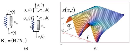
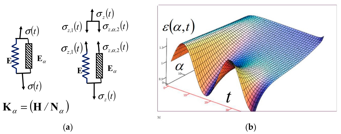
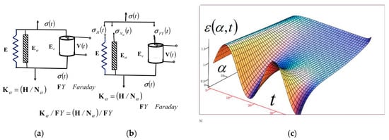
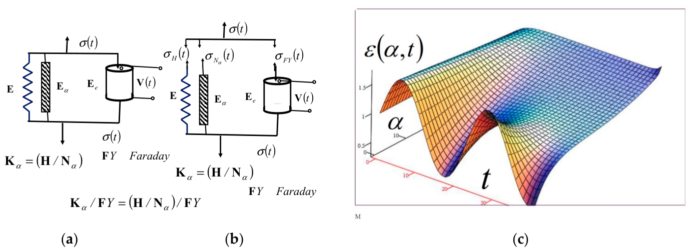
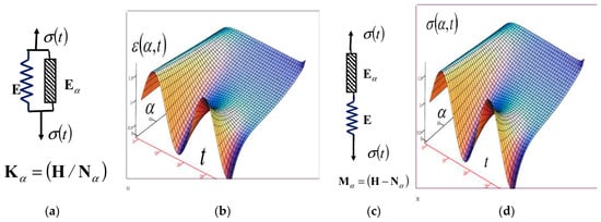
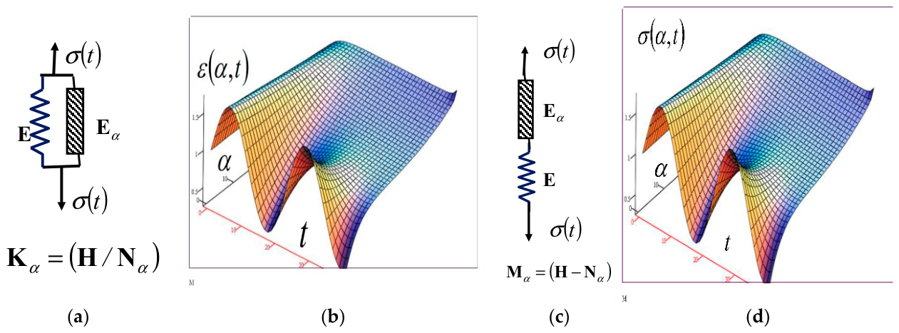
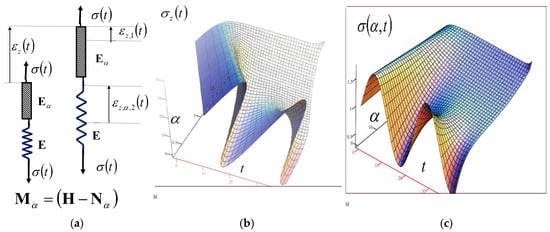
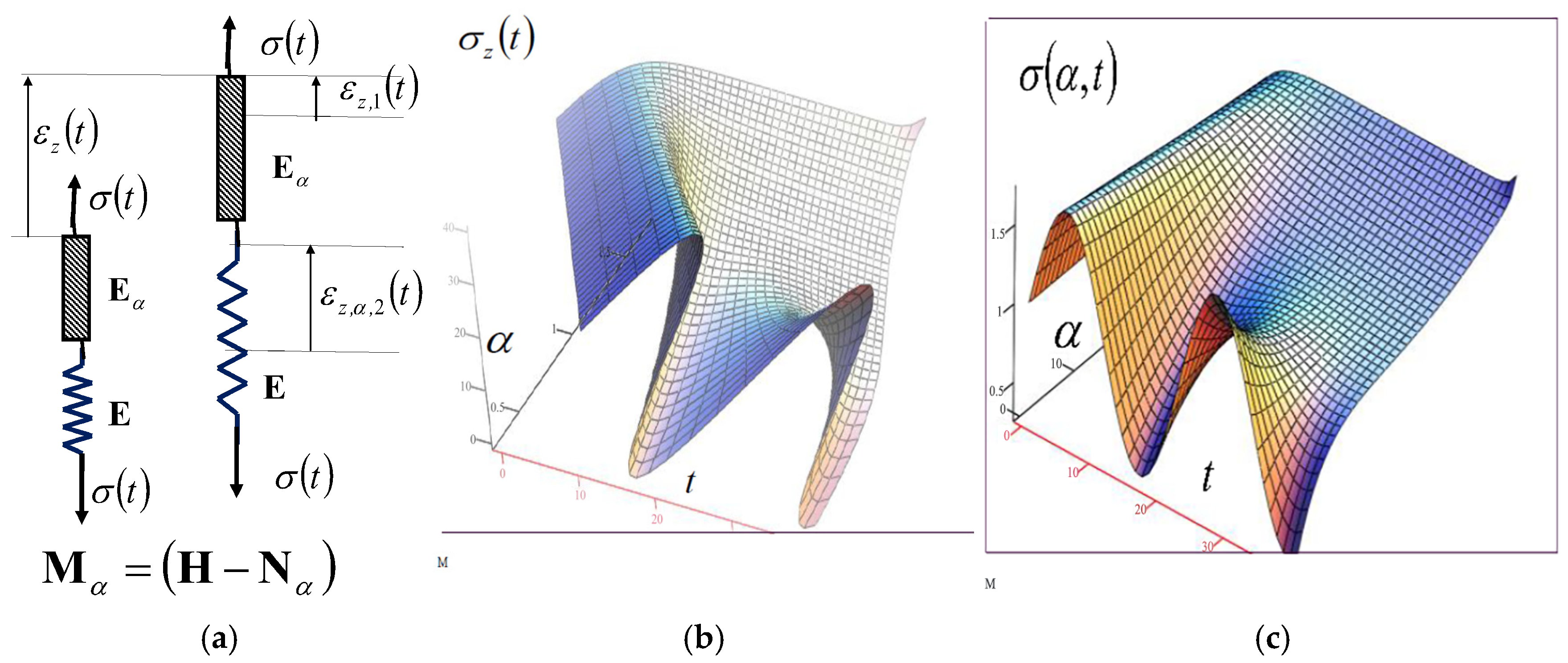
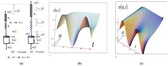
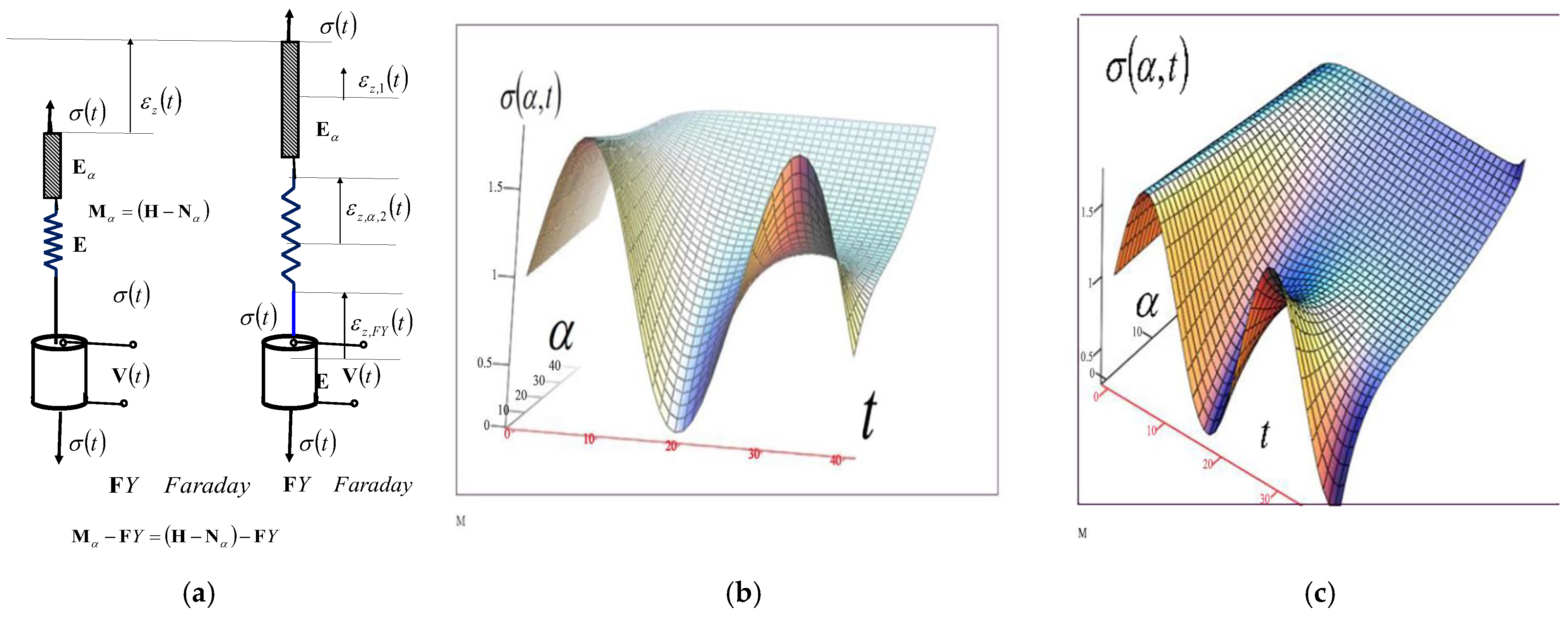
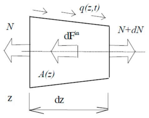
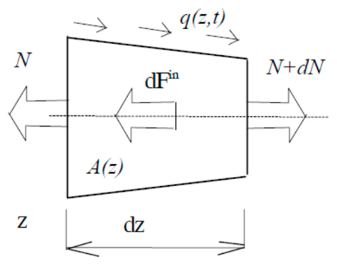
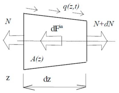
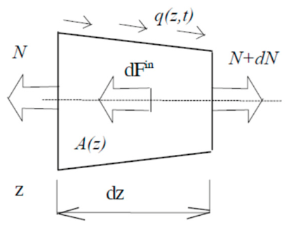
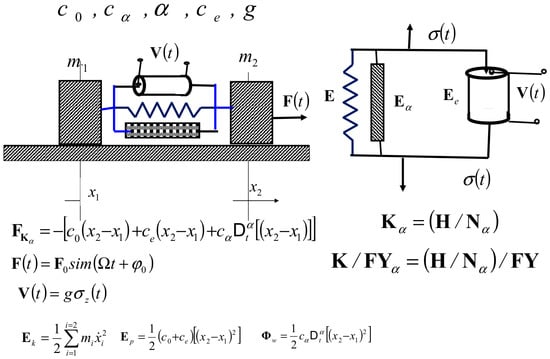
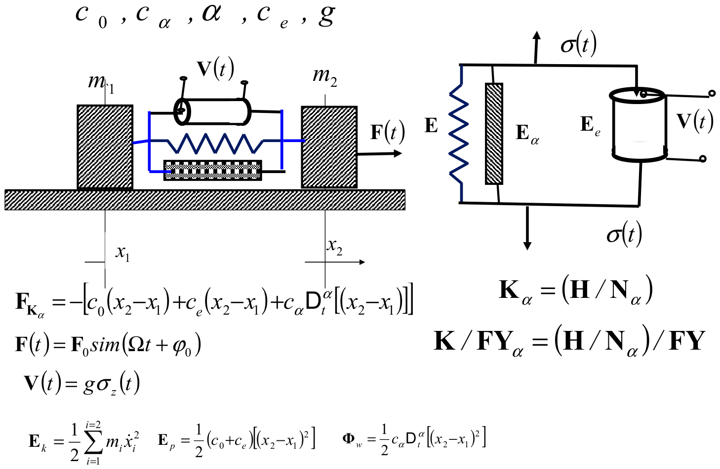
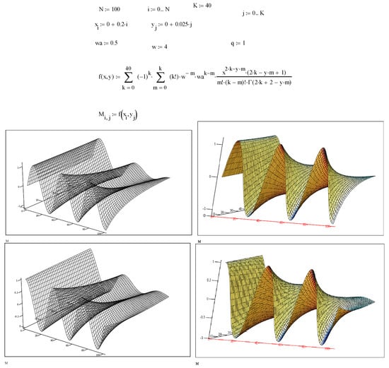
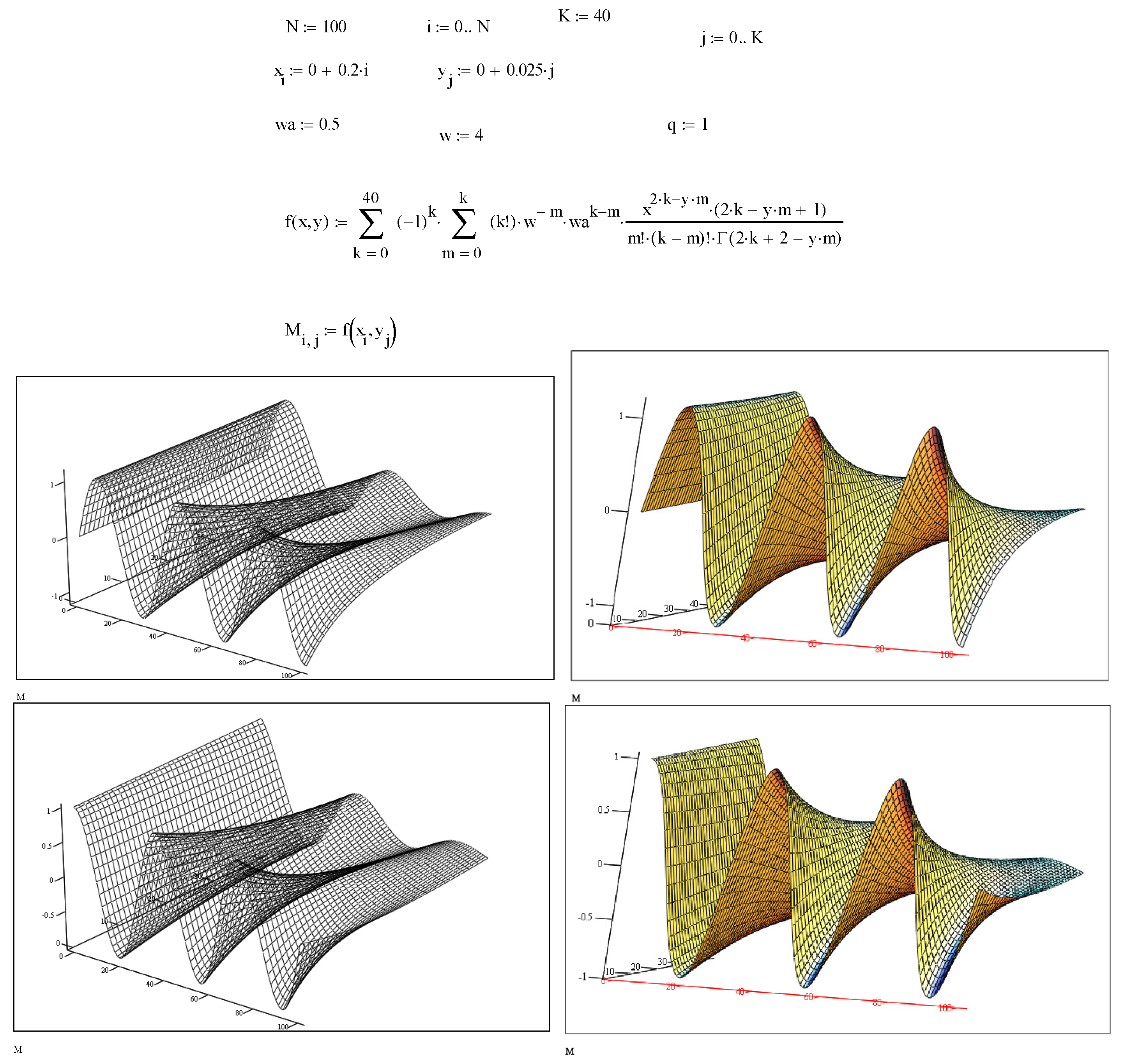
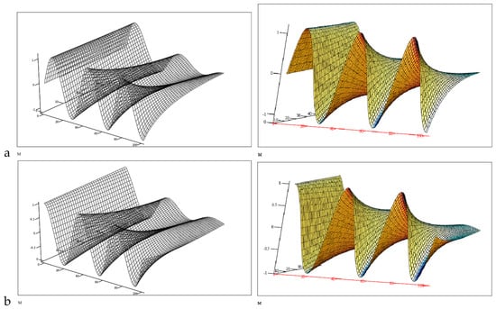
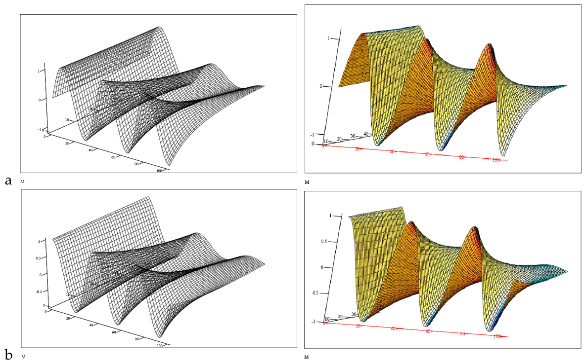
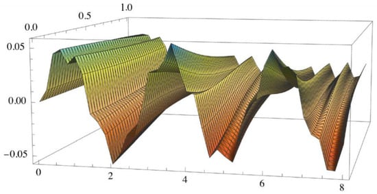
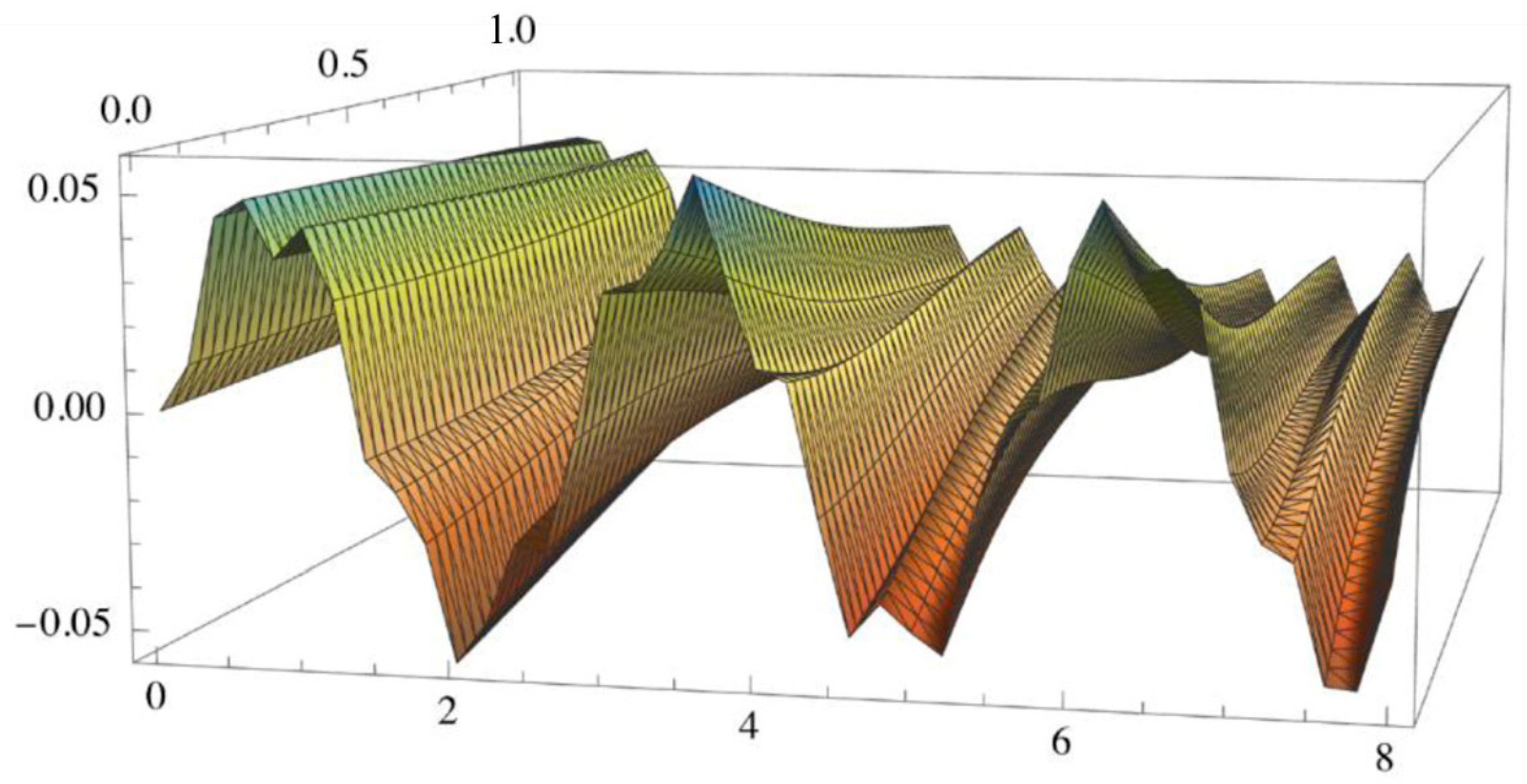
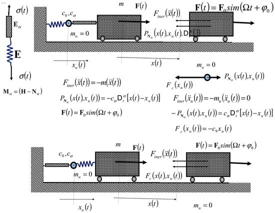
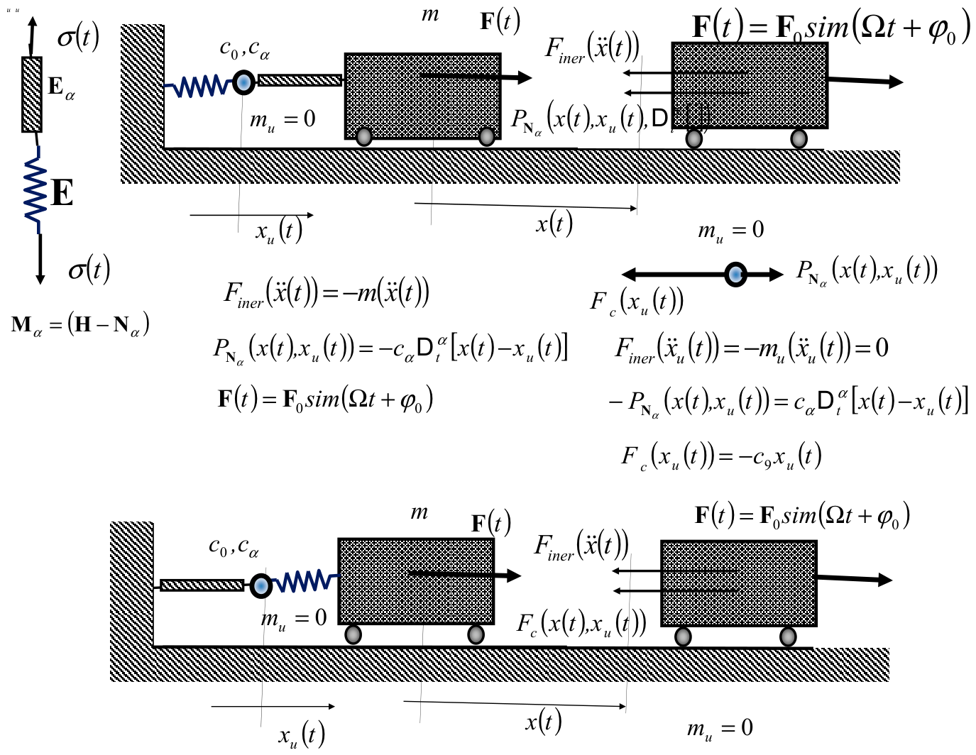
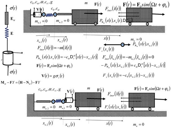
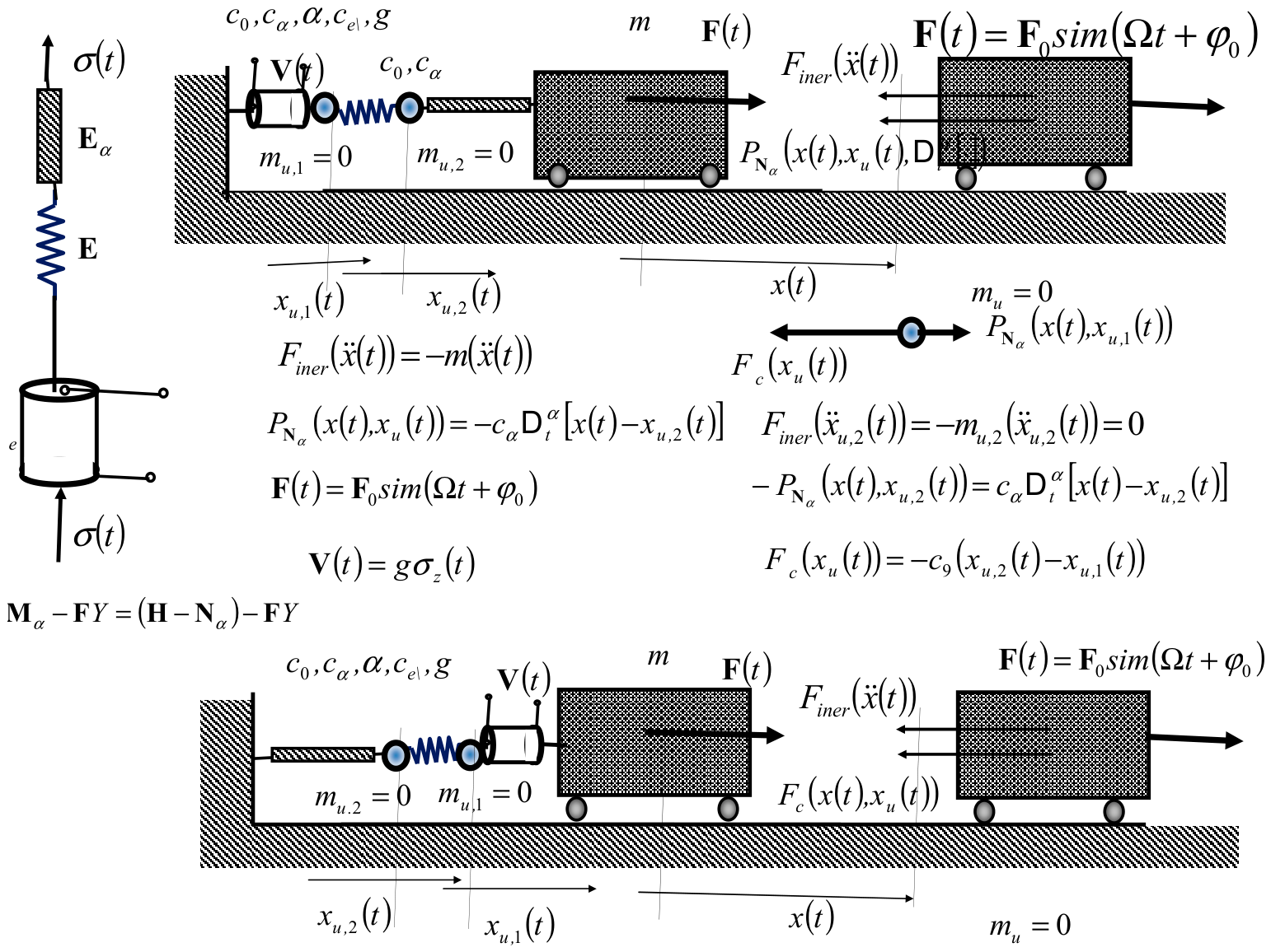

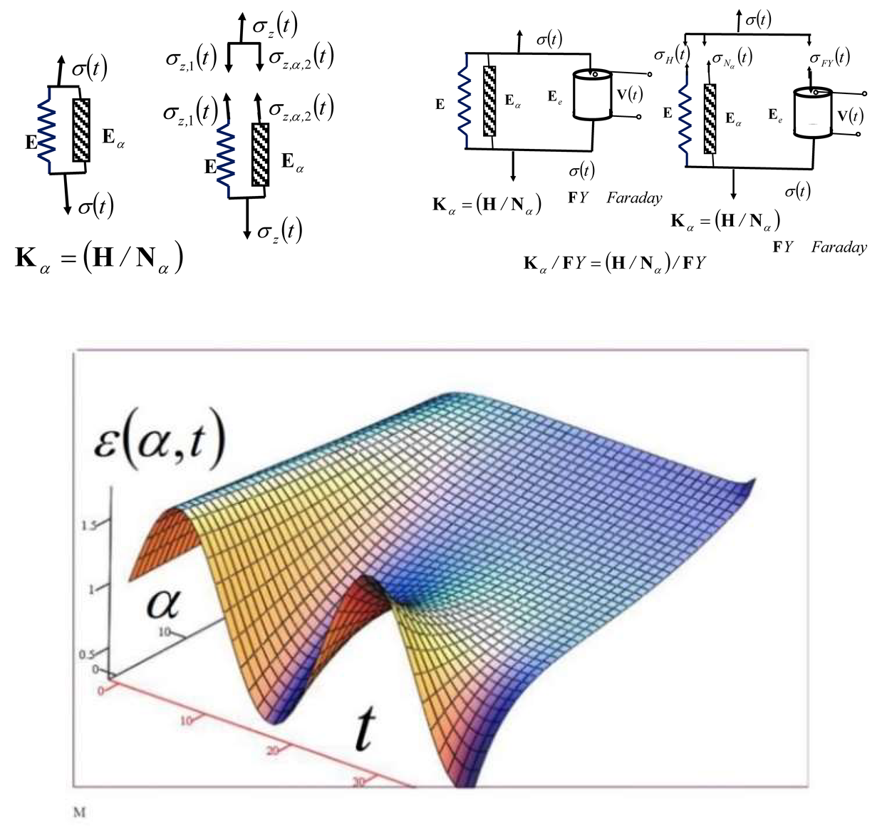
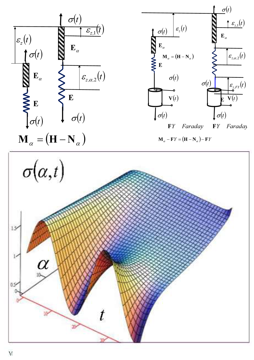
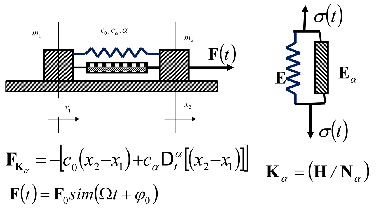
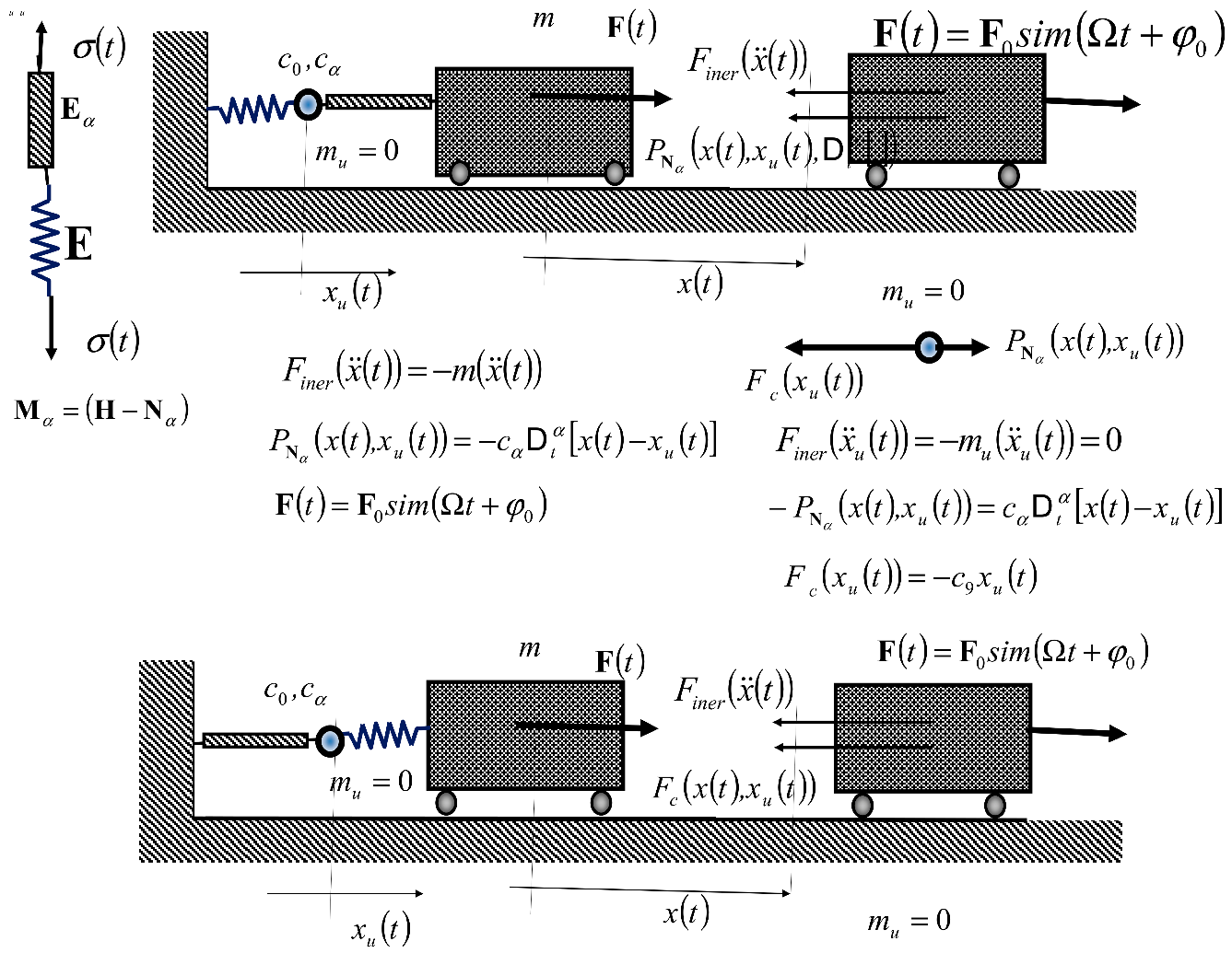
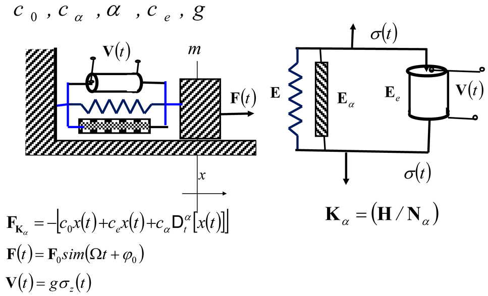
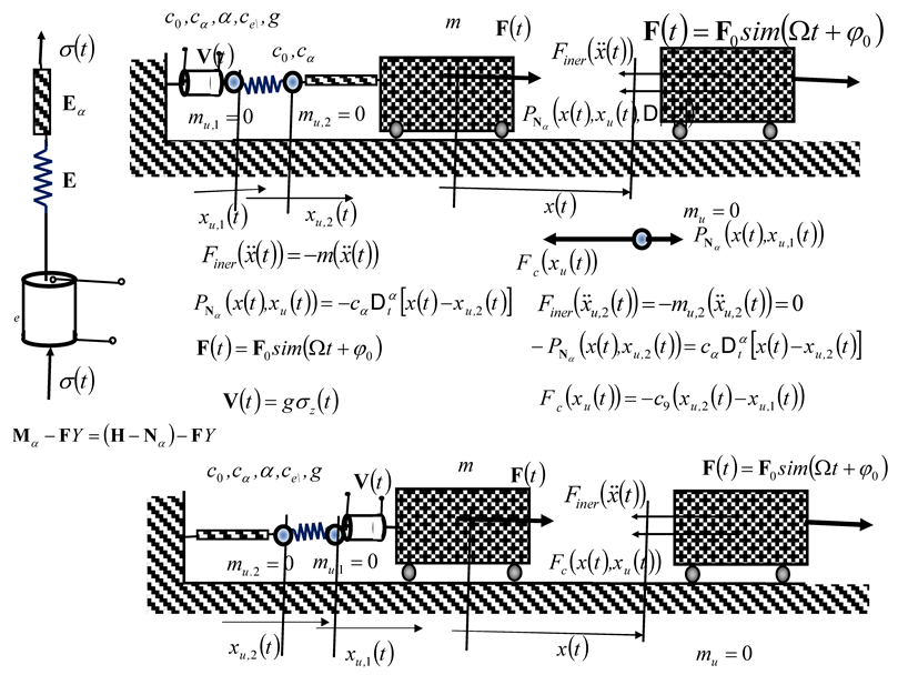
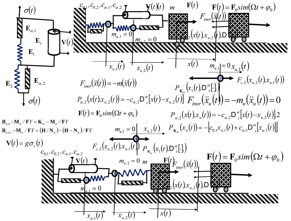
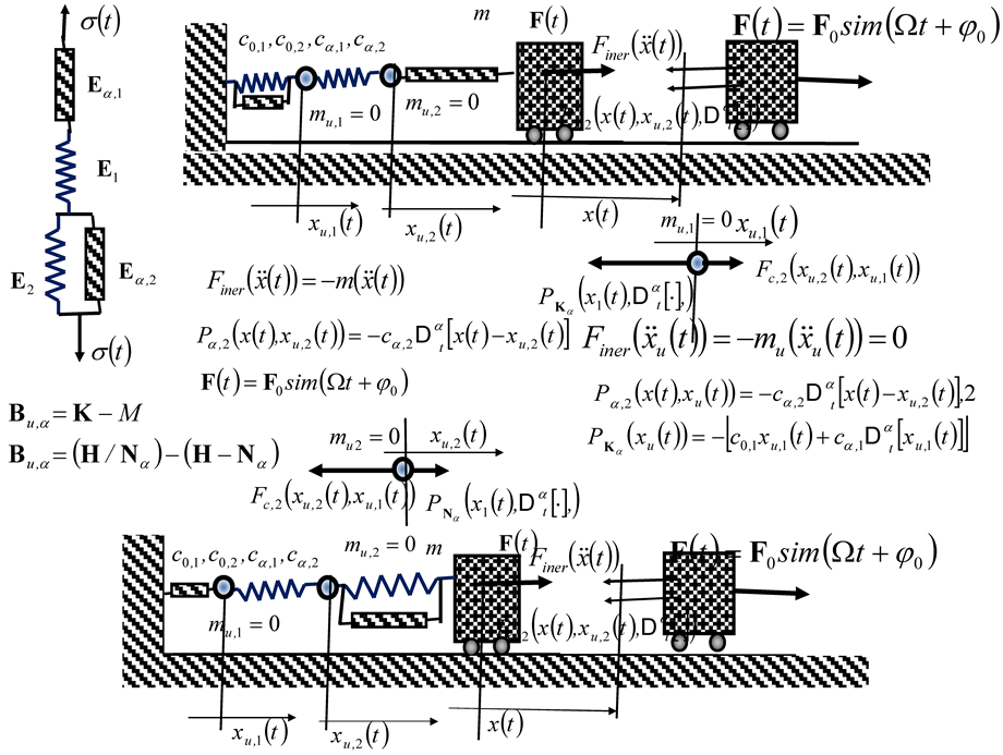
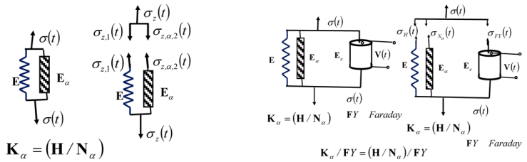
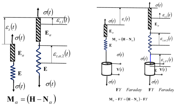
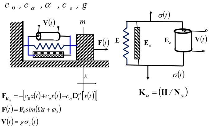
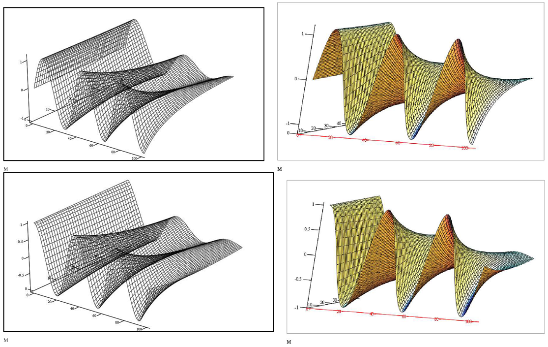
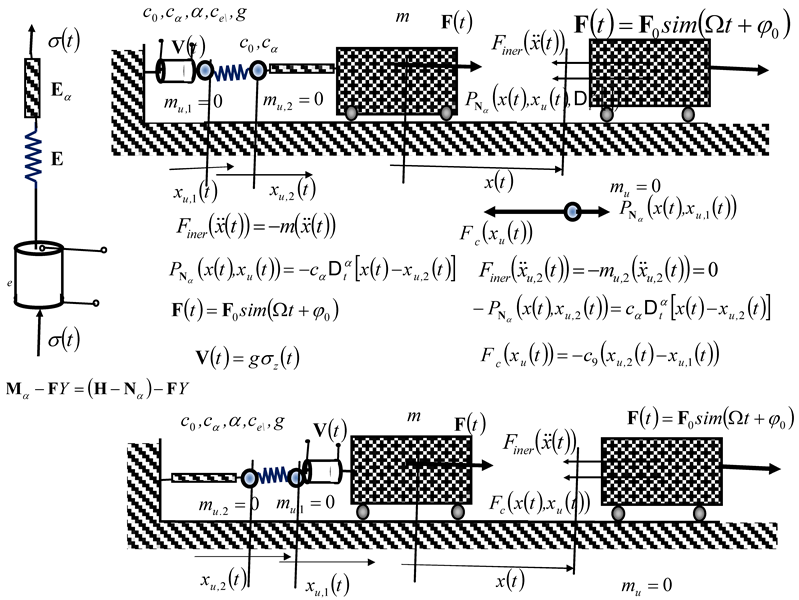
Disclaimer/Publisher’s Note: The statements, opinions and data contained in all publications are solely those of the individual author(s) and contributor(s) and not of MDPI and/or the editor(s). MDPI and/or the editor(s) disclaim responsibility for any injury to people or property resulting from any ideas, methods, instructions or products referred to in the content. |
© 2026 by the author. Licensee MDPI, Basel, Switzerland. This article is an open access article distributed under the terms and conditions of the Creative Commons Attribution (CC BY) license.