Bayesian Additive Regression Trees for Circular Data: A Machine Learning Framework

Abstract

Circular data arise in a wide range of scientific fields, including meteorology, medicine, biology, and neuroscience, yet existing regression methods for such data are largely restricted to parametric generalized linear models or tree-based methods that impose distributional assumptions on the circular response. In this paper, we propose a family of Bayesian Additive Regression Tree (BART) methods for regression with circular data, covering three cases: Circular–Circular BART (CCBART), where both the response and the covariates are circular; Circular–Linear BART (CLBART), where the response is circular and the covariates are linear; and Linear–Circular BART (LCBART), where the response is linear and the covariates are circular. The proposed methods adopt a projection approach, decomposing circular variables into their sine and cosine components, fitting separate BART models on these projections, and recovering circular predictions via the two-argument arctangent function. This avoids specifying a von Mises or wrapped normal likelihood directly for the circular response, though it does not avoid all distributional assumptions: BART assumes flexible Euclidean regression models, with Gaussian errors, for the projected sine and cosine components. The approach retains the full inferential power of BART, including posterior uncertainty quantification, automatic variable selection, and the ability to capture nonlinear effects and interactions without pre-specification. An extensive simulation study demonstrates that the proposed methods are highly competitive with random forest benchmarks and consistently outperform linear model benchmarks, with the clearest and most consistent advantage over random forests emerging at high noise levels and in the Linear–Circular case, where LCBART achieves up to 34% lower RMSE than projected random forests. Applications to wind direction forecasting and human motor resonance data further illustrate the practical utility of the proposed methods.

1. Introduction

Regression modelling with circular data presents unique statistical challenges that are not addressed by standard linear methods. Circular variables—such as wind direction, time of day, and biological orientation angles—are periodic in nature, meaning that values near 0 and $2\pi$ are arbitrarily close rather than far apart. This periodicity invalidates the standard assumptions of linear regression and requires specialized methods. Despite the wide occurrence of circular data across meteorology, medicine, biology, neuroscience, and other fields, the development of flexible nonparametric regression methods for circular data remains limited compared to the linear setting. In this paper, we address this gap by proposing a family of Bayesian Additive Regression Tree (BART) methods for regression with circular data, covering three distinct cases depending on whether the response variable, the covariates, or both are circular. The remainder of the introduction reviews the relevant background in directional statistics, circular regression, and BART before examining the proposed approach.

1.1. Directional Statistics

Directional statistics is a branch of statistics that deals with data that are directions. Usually, directional data lie on the circumference of the unit circle or on the unit hypersphere (for more, see [1,2]). The first known statistical analysis of directional data was at the beginning of the 19th century by [3]. Later, the development of the methods of directional statistics continued in the 20th century mainly by Langevin [4], Lévy [5], Fisher [6]. Directional statistics have become increasingly applied across diverse fields in recent years, including animal behavior [7], wind direction analysis [8], flooding modelling [9], and text mining [10]. A comprehensive review of recent developments in directional statistics, covering distributional models, hypothesis testing, regression, nonparametric curve estimation, and machine learning, is provided by Pewsey and García-Portugués [11], who highlight applications in fields as diverse as astronomy, medicine, genetics, neurology, environmetrics, and image analysis.

Circular Regression

Regression models for circular data have a long history. One of the earliest contributions was by Gould [12], who proposed a regression technique for angular variates using the von Mises distribution. Fisher and Lee [13] extended this by introducing generalized linear model (GLM)-type approaches for a circular response with either circular or linear covariates, using a tangent link function to ensure periodicity. Specifically, for a circular response $\theta$ and linear covariates x, the conditional mean direction $\mu$ is modeled as

$$\begin{array}{c}\hfill \mu ={\mu }_0+2{\tan }^{-1}\left({\beta }^{T}x\right),\end{array}$$

where ${\mu }_0$ is a circular intercept and $\beta$ is a vector of regression coefficients. Sarma and Jammalamadaka [14] proposed a generic Circular–Circular regression by jointly modelling the sine and cosine of the angular response on a trigonometric polynomial of the angular covariate $\mathrm{\Theta }$,

$$\begin{array}{cc}\hfill \sin \left(\theta \right)& ={\displaystyle \sum _{k=1}^q}\left(a_k\cos \left(k\mathrm{\Theta }\right)+b_k\sin \left(k\mathrm{\Theta }\right)\right)+{ϵ}_1,\hfill \\ \hfill \cos \left(\theta \right)& ={\displaystyle \sum _{k=1}^q}\left(c_k\cos \left(k\mathrm{\Theta }\right)+d_k\sin \left(k\mathrm{\Theta }\right)\right)+{ϵ}_2,\hfill \end{array}$$

where q is the order of the trigonometric polynomial and $a_k,b_k,c_k,$ and $d_k$ are regression coefficients. Throughout this paper, $\mathrm{atan2}(y,x)$ denotes the two-argument arctangent function returning the angle of the point $(x,y)$ in the plane, following the common software convention (e.g., R, version 4.5.1) in which the first argument is the sine (ordinate) component and the second is the cosine (abscissa) component, so that $\mathrm{atan2}(\sin \theta ,\cos \theta )=\theta$ (modulo $2\pi$). The circular response is then recovered as

$$\begin{array}{c}\hfill \widehat{\theta }=\mathrm{atan2}\left(\widehat{\sin \left(\theta \right)},\widehat{\cos \left(\theta \right)}\right)\left(\mathrm{mod}2\pi \right).\end{array}$$

Further developments include rotational models by [15,16] based on Möbius transformations, multivariate circular regression by Kim and SenGupta [17], and circular regression models for animal movements by Rivest et al. [18].

Despite their theoretical elegance, GLM-based circular regression models present practical difficulties. As noted by Presnell et al. [19], maximum likelihood estimation of their parameters is prone to numerical instability due to the non-concavity of the log-likelihood. Furthermore, the nonlinear link function makes interpretation of covariate effects challenging, and the additive model structure may fail to capture abrupt changes or interactions, which are common in applications such as wind direction forecasting. Lang et al. [20] addressed some of these limitations by proposing circular regression trees and forests based on the von Mises distribution and recursive partitioning, which can automatically detect nonlinear effects and interactions without requiring a link function. More recently, Marques F. et al. [21] proposed projected random forests for circular responses, applying the projection approach of [14] to random forests by fitting two separate models

$$\begin{array}{cc}\hfill \sin \left(\theta \right)& =f_1\left(x\right)+{ϵ}_1,\hfill \\ \hfill \cos \left(\theta \right)& =f_2\left(x\right)+{ϵ}_2,\hfill \end{array}$$

where $f_1$ and $f_2$ are random forest models, and recovering the circular prediction via

$$\begin{array}{c}\hfill \widehat{\theta }=\mathrm{atan2}\left({\widehat{f}}_1\left(x\right),{\widehat{f}}_2\left(x\right)\right)\left(\mathrm{mod}2\pi \right).\end{array}$$

1.2. Bayesian Additive Regression Trees

Suppose we have p covariates $x=(x_1,\dots ,x_p)$ and response y. Consider the problem of making inference about an unknown function f that predicts y using x

$$\begin{array}{c}\hfill y=f\left(x\right)+ϵ,ϵ\sim N(0,{\sigma }^2).\end{array}$$

To do this, Chipman et al. [22] considered approximating the mean of y given x, $f\left(x\right)=E\left(y\right|x)$, using the sum of m regression trees

$$\begin{array}{c}\hfill f\left(x\right)\approx h\left(x\right)={\displaystyle \sum _{j=1}^m}{g}_j\left(x\right),\end{array}$$

where $g_j$ denotes the jth tree. Regularization is achieved through a prior on the tree structures and terminal node parameters. Specifically, each tree is encouraged to be shallow via the prior probability that a node at depth d is non-terminal, given by $\alpha {(1+d)}^{-\beta }$ with defaults $\alpha =0.95$ and $\beta =2$, and the terminal node parameters ${\mu }_{ij}$ are assigned a normal prior ${\mu }_{ij}\sim N(0,{\sigma }_{\mu }^2)$ where ${\sigma }_{\mu }=0.5/\left(k\sqrt{m}\right)$ for a shrinkage parameter k. The error variance is assigned an inverse chi-squared prior ${\sigma }^2\sim \nu \lambda /{\chi }_{\nu }^2$. Together, these priors ensure that each tree contributes only a small part of the overall fit, so that no single tree dominates. Fitting and inference are accomplished via a Bayesian backfitting MCMC algorithm that iteratively samples each tree from its conditional posterior given the partial residuals from all other trees, generating draws from the joint posterior $p((T_1,M_1),\dots ,(T_m,M_m),\sigma \mid y)$. Point estimates of $f\left(x\right)$ are obtained as the posterior mean across MCMC draws, and posterior uncertainty intervals are obtained from the corresponding quantiles.

BART has several appealing features: it is robust to the choice of tuning parameters, provides full posterior uncertainty quantification, performs automatic variable selection by tracking predictor inclusion frequencies, and captures nonlinear effects and interactions without requiring their pre-specification. Chipman et al. [22] demonstrated that BART compares favorably with boosting, random forests, and neural networks across 42 real datasets. Since its introduction, BART has been extended and applied widely, including in variable selection [23], survival analysis [24], causal inference [25], and skewed responses [26].

1.3. Motivation

Despite the growing importance of circular data in applied statistics and the demonstrated effectiveness of BART as a nonparametric regression tool, no existing work adapts BART to the projection-based framework for circular regression. Our contribution is best characterized as a computational and methodological adaptation of BART to this existing framework; we discuss the resulting statistical implications, in Section 2.4. Current circular regression methods are largely restricted to parametric GLM frameworks or tree-based methods using the von Mises distribution, both of which impose distributional assumptions on the response and struggle with nonlinear covariate effects, interactions, and high-dimensional predictor spaces. In this paper, we address this gap by proposing a family of BART-based methods for regression with circular data. Following the projection approach of [13,21], we decompose circular variables into their sine and cosine components, fit separate BART models, and recover circular predictions via $\mathrm{atan2}(·,·)$. This avoids specifying a von Mises or wrapped normal likelihood directly for the circular response; it does not, however, avoid all distributional assumptions, since BART itself assumes Gaussian errors for the projected sine and cosine components, which are bounded in $[-1,1]$. A more precise characterization of the method is that it uses a flexible Euclidean regression model for the projected components rather than a direct parametric circular likelihood for $\theta$ (see Section 2.4 for further discussion). The approach retains the full inferential power of BART, including uncertainty quantification and variable selection. We consider three cases: both response and covariates being circular (CCBART), a circular response with linear covariates (CLBART), and a linear response with circular covariates (LCBART). The performance of the proposed methods is assessed through an extensive simulation study and real-data applications to wind direction forecasting and human motor resonance data.

2. Methodology

In this section, we present methods for incorporating circular data into BART. The key idea is to avoid modelling circular variables directly, which would require parametric distributional assumptions and link functions to handle periodicity. Instead, we adopt a projection approach: circular variables are decomposed into their sine and cosine components, standard BART models are fitted on these projections, and circular predictions are recovered via the two-argument arctangent function $\mathrm{atan2}(·,·)$. This idea was used in the context of circular regression by [13] and extended to random forests by [21]; here, we extend it to BART for the first time. This extension is computational and methodological in nature: fitting the sine and cosine components independently, as in [13,21]. We characterize the resulting estimator’s properties formally in Section 2.4 and address the independence assumption empirically in Section 2.5. In all cases, ${ϵ}_1,{ϵ}_2,ϵ\sim N(0,{\sigma }^2)$ independently, consistent with the projected normal distribution on the circle, and predictions are obtained using the posterior mean of the fitted BART models.

2.1. Circular–Circular BART

We propose Circular–Circular BART (CCBART) for the case where both the response and the covariates are circular. Let $\theta$ be the response variable and $({\mathrm{\Theta }}_1,\dots ,{\mathrm{\Theta }}_p)$ be the covariates, where $\theta$ and each ${\mathrm{\Theta }}_j$ are angles with $0\le \theta ,{\mathrm{\Theta }}_j\le 2\pi$. To handle the periodicity of both the response and the covariates, we decompose all circular variables into their sine and cosine components and fit two separate BART models:

$$\begin{array}{cc}\hfill \sin \left(\theta \right)& =f_1(\sin \left({\mathrm{\Theta }}_1\right),\cos \left({\mathrm{\Theta }}_1\right),\dots ,\sin \left({\mathrm{\Theta }}_p\right),\cos \left({\mathrm{\Theta }}_p\right))+{ϵ}_1,\hfill \\ \hfill \cos \left(\theta \right)& =f_2(\sin \left({\mathrm{\Theta }}_1\right),\cos \left({\mathrm{\Theta }}_1\right),\dots ,\sin \left({\mathrm{\Theta }}_p\right),\cos \left({\mathrm{\Theta }}_p\right))+{ϵ}_2.\hfill \end{array}$$

The response is then predicted as

$$\begin{array}{c}\hfill \widehat{\theta }=\mathrm{atan2}\left(\widehat{\sin \left(\theta \right)},\widehat{\cos \left(\theta \right)}\right)\left(\mathrm{mod}2\pi \right).\end{array}$$

2.2. Circular–Linear BART

We propose Circular–Linear BART (CLBART) for the case where the response is circular and the covariates are linear. Let $\theta$ be the response variable with $0\le \theta \le 2\pi$, and let $(x_1,\dots ,x_p)$ be linear covariates. Only the response requires decomposition, and we fit two BART models:

$$\begin{array}{cc}\hfill \sin \left(\theta \right)& =f_1(x_1,\dots ,x_p)+{ϵ}_1,\hfill \\ \hfill \cos \left(\theta \right)& =f_2(x_1,\dots ,x_p)+{ϵ}_2.\hfill \end{array}$$

The response is then predicted as

$$\begin{array}{c}\hfill \widehat{\theta }=\mathrm{atan2}\left(\widehat{\sin \left(\theta \right)},\widehat{\cos \left(\theta \right)}\right)\left(\mathrm{mod}2\pi \right).\end{array}$$

2.3. Linear–Circular BART

We propose Linear–Circular BART (LCBART) for the case where the response is linear and the covariates are circular. Let y be the response variable and $({\mathrm{\Theta }}_1,\dots ,{\mathrm{\Theta }}_p)$ be the covariates, where each ${\mathrm{\Theta }}_j$ is an angle with $0\le {\mathrm{\Theta }}_j\le 2\pi$. Only the covariates require decomposition, and we fit the BART model

$$\begin{array}{cc}\hfill y& =f(\sin \left({\mathrm{\Theta }}_1\right),\cos \left({\mathrm{\Theta }}_1\right),\dots ,\sin \left({\mathrm{\Theta }}_p\right),\cos \left({\mathrm{\Theta }}_p\right))+ϵ.\hfill \end{array}$$

The response is predicted as the posterior mean $\widehat{y}=\widehat{f}(\sin \left(\mathrm{\Theta }\right),\cos \left(\mathrm{\Theta }\right))$.

Algorithm 1 summarizes the common fitting and prediction procedure across the three model variants defined above.

2.4. Theoretical Properties

While the primary contribution of this paper is methodological, we establish here several basic properties of the proposed projection-based construction. Throughout, let $x\in \mathcal{X}\subset {\mathbb{R}}^p$ and let $\theta \left(x\right)\in [0,2\pi )$ denote the true circular regression function, with projected components $f_1\left(x\right)=\sin \theta \left(x\right)$ and $f_2\left(x\right)=\cos \theta \left(x\right)$. Let ${\widehat{f}}_1,{\widehat{f}}_2$ denote estimators of $f_1,f_2$ obtained by fitting two regression models independently (e.g., via BART), and define the induced angle estimator $\widehat{\theta }\left(x\right)=\mathrm{atan2}({\widehat{f}}_1\left(x\right),{\widehat{f}}_2\left(x\right))$ and the resultant length $r\left(x\right)=\sqrt{{\widehat{f}}_1{\left(x\right)}^2+{\widehat{f}}_2{\left(x\right)}^2}$.

Proposition 1 

(Scale non-identifiability of the angle estimator). For any $c>0$, $\mathrm{atan2}(c{\widehat{f}}_1\left(x\right),c{\widehat{f}}_2\left(x\right))=\mathrm{atan2}({\widehat{f}}_1\left(x\right),{\widehat{f}}_2\left(x\right))$. Consequently, $\widehat{\theta }\left(x\right)$ does not identify $r\left(x\right)$: any two estimators $({\widehat{f}}_1,{\widehat{f}}_2)$ and $(c{\widehat{f}}_1,c{\widehat{f}}_2)$, where $c>0$, yield the same $\widehat{\theta }\left(x\right)$ but different $r\left(x\right)$.

Proof. 

By definition, $\mathrm{atan2}(y,x)$ returns the angle of the ray from the origin through $(x,y)$. Scaling $(x,y)$ by $c>0$ preserves the ray and hence the angle. Thus, $\widehat{\theta }\left(x\right)$ is a function only of the direction of $({\widehat{f}}_1\left(x\right),{\widehat{f}}_2\left(x\right))$, not its magnitude, while $r\left(x\right)$ depends only on the magnitude. □

Remark 1. 

This formally justifies reporting $r\left(x\right)$ separately from $\widehat{\theta }\left(x\right)$: the point prediction alone cannot reveal how close the underlying estimator is to the unit circle, since this information is invariant under rescaling and therefore invisible to $\mathrm{atan2}$.

Algorithm 1: Fitting and prediction for CCBART, CLBART, and LCBART

Input: training data ${\left\{{(}_i,{\theta }_i)\right\}}_{i=1}^n$ (or $\left\{{(}_i,y_i)\right\}$ for LCBART); number of trees m; posterior draws $\mathtt{ndpost}$; burn-in $\mathtt{nskip}$. Encode circular variables. Replace each circular covariate ${\mathrm{\Theta }}_j$ by the pair $(\sin {\mathrm{\Theta }}_j,\cos {\mathrm{\Theta }}_j)$. For CCBART and CLBART, also form the circular response targets $\sin \left({\theta }_i\right)$ and $\cos \left({\theta }_i\right)$. Fit component model(s). (a) For CCBART and CLBART: fit two independent BART models, $f_1$ on target $\sin \left({\theta }_i\right)$ and $f_2$ on target $\cos \left({\theta }_i\right)$, each with m trees, using the encoded covariates from Step 1. (b) For LCBART: fit a single BART model f on target $y_i$, using the encoded circular covariates from Step 1. Run MCMC. For each model, run the Bayesian backfitting Gibbs sampler for $\mathtt{nskip}+\mathtt{ndpost}$ iterations, discarding the first $\mathtt{nskip}$ as burn-in and retaining $\mathtt{ndpost}$ post-burn-in draws. Predict. (a) For CCBART and CLBART: at a new point *, compute the posterior mean predictions ${\widehat{f}}_1{(}^{*})$, ${\widehat{f}}_2{(}^{*})$, and recover the predicted direction as $\widehat{\theta }{(}^{*})=\mathrm{atan2}({\widehat{f}}_1{(}^{*}),{\widehat{f}}_2{(}^{*}))\left(\mathrm{mod}2\pi \right)$. Report the resultant length $r{(}^{*})=\sqrt{{\widehat{f}}_1{{(}^{*})}^2+{\widehat{f}}_2{{(}^{*})}^2}$ as a diagnostic (Section 2.4), together with the normalized score vector $\widehat{v}{(}^{*})=({\widehat{f}}_1{(}^{*}),{\widehat{f}}_2{(}^{*}))/r{(}^{*})$, a genuine point on the unit circle reported for interpretability; by Proposition 1, $\widehat{\theta }{(}^{*})$ is unaffected by whether it is computed from $({\widehat{f}}_1{(}^{*}),{\widehat{f}}_2{(}^{*}))$ or from $\widehat{v}{(}^{*})$. (b) For LCBART: at a new point *, compute the posterior mean prediction $\widehat{y}{(}^{*})=\widehat{f}{(}^{*})$ directly. (CCBART, CLBART only) Assess and correct for component dependence. Estimate the residual covariance $\widehat{\Sigma }$ between the fitted sine and cosine components on held-out data (Section 2.5), and use $\widehat{\Sigma }$ to draw correlated predictive noise when constructing posterior credible arcs (Section 2.7). Output: predicted direction $\widehat{\theta }{(}^{*})$ (or value $\widehat{y}{(}^{*})$), posterior credible arc (or interval), and diagnostics $r{(}^{*})$, $\widehat{\rho }$.

In addition to reporting $r\left(x\right)$, we report the normalized score vector

$$\widehat{v}\left(x\right)={\displaystyle \frac{({\widehat{f}}_1\left(x\right),{\widehat{f}}_2\left(x\right))}{r\left(x\right)}},\mathrm{whenever}r\left(x\right)>0,$$

which is a genuine point on the unit circle, distinct from the possibly off-circle raw pair $({\widehat{f}}_1\left(x\right),{\widehat{f}}_2\left(x\right))$. By Proposition 1, $\mathrm{atan2}({\widehat{v}}_1\left(x\right),{\widehat{v}}_2\left(x\right))=\widehat{\theta }\left(x\right)$, so normalization changes neither the predicted angle nor its interpretation as a ray direction; we report $\widehat{v}\left(x\right)$ purely as an interpretable diagnostic representation of the estimated direction on the circle, alongside $r\left(x\right)$.

Proposition 2 

(Conditional consistency of the induced angle estimator under the geodesic metric). Suppose ${\widehat{f}}_1\left(x\right)\stackrel{p}{\to }{f}_1\left(x\right)$ and ${\widehat{f}}_2\left(x\right)\stackrel{p}{\to }{f}_2\left(x\right)$ as $n\to \infty$, for some x with $f_1{\left(x\right)}^2+f_2{\left(x\right)}^2>0$. Let $d(\alpha ,\beta )=1-\cos (\alpha -\beta )$ denote the geodesic distance on ${\mathbb{S}}^1$. Then $d(\widehat{\theta }\left(x\right),\theta \left(x\right))\stackrel{p}{\to }0$.

Proof. 

Write $\mathbf{u}=(f_1\left(x\right),f_2\left(x\right))/\parallel (f_1\left(x\right),f_2\left(x\right))\parallel$ and $\widehat{\mathbf{u}}=({\widehat{f}}_1\left(x\right),{\widehat{f}}_2\left(x\right))/\parallel ({\widehat{f}}_1\left(x\right),{\widehat{f}}_2\left(x\right))\parallel$, the projections of the true and estimated component pairs onto ${\mathbb{S}}^1$. Since $(f_1\left(x\right),f_2\left(x\right))\ne (0,0)$ by assumption, the map $(y_1,y_2)\mapsto (y_1,y_2)/\parallel (y_1,y_2)\parallel$ is continuous at the limit point $(f_1\left(x\right),f_2\left(x\right))$. By the continuous mapping theorem, $\widehat{\mathbf{u}}\stackrel{p}{\to }\mathbf{u}$. Since $d(\widehat{\theta }\left(x\right),\theta \left(x\right))=1-\widehat{\mathbf{u}}·\mathbf{u}$ is a continuous function of $\widehat{\mathbf{u}}$ for fixed $\mathbf{u}$, with value 0 at $\widehat{\mathbf{u}}=\mathbf{u}$, a further application of the continuous mapping theorem gives $d(\widehat{\theta }\left(x\right),\theta \left(x\right))\stackrel{p}{\to }0$. □

Remark 2. 

Convergence is stated under the geodesic distance d on ${\mathbb{S}}^1$ rather than ordinary Euclidean distance on the coordinate representative $\theta \in [0,2\pi )$, since any such coordinate representative requires an arbitrary cut point (here, $\theta =0\equiv 2\pi$) at which Euclidean convergence of $\widehat{\theta }\left(x\right)$ to $\theta \left(x\right)$ can fail even when the underlying directions converge. The geodesic metric d carries no such artefact, since ${\mathbb{S}}^1$ itself has no boundary. As in Proposition 1, the hypothesis is stated as a conditional on the components’ consistency, since verifying it requires the technical conditions of existing BART posterior-consistency results [27,28] applied component-wise to $f_1,f_2$; we do not re-derive these here. The result fails, or degrades, precisely as $\sqrt{f_1{\left(x\right)}^2+f_2{\left(x\right)}^2}\to 0$, the same instability region monitored empirically via $r\left(x\right)$.

Proposition 3 

(A bound on the constraint-violation diagnostic). Let $\Delta \left(x\right)=\left|r\right(x)-1|$. Suppose ${\widehat{f}}_1\left(x\right)$ and ${\widehat{f}}_2\left(x\right)$ are unbiased with variances ${\sigma }_1^2\left(x\right)$ and ${\sigma }_2^2\left(x\right)$, and finite higher-order moments. Then, for ${\sigma }_1^2\left(x\right)$ and ${\sigma }_2^2\left(x\right)$, sufficiently small,

$$\mathbb{E}\left[\Delta {\left(x\right)}^2\right]\lesssim {\sigma }_1^2\left(x\right)+{\sigma }_2^2\left(x\right).$$

Proof. 

Write ${\widehat{f}}_1=f_1+{\epsilon }_1$, ${\widehat{f}}_2=f_2+{\epsilon }_2$ with $\mathbb{E}\left[{\epsilon }_k\right]=0$, $\mathrm{Var}\left({\epsilon }_k\right)={\sigma }_k^2\left(x\right)$, and $f_1^2+f_2^2=1$. Then

$$r{\left(x\right)}^2-1=2f_1{\epsilon }_1+2f_2{\epsilon }_2+{\epsilon }_1^2+{\epsilon }_2^2.$$

Since $r\left(x\right)\ge 0$, we have $r\left(x\right)+1\ge 1$, and therefore $\Delta \left(x\right)=\left|r\right(x)-1|\le \left|r\right(x)-1|\left(r\right(x)+1)$${=|r\left(x\right)}^2-1|$. Using $|f_1|,|f_2|\le 1$, using expectations of the square of the right-hand side above and retaining the leading-order variance terms (assuming bounded higher-order moments of ${\epsilon }_k$, so that third- and fourth-order moment terms are dominated by ${\sigma }_1^2\left(x\right)+{\sigma }_2^2\left(x\right)$ as ${\sigma }_1^2\left(x\right),{\sigma }_2^2\left(x\right)\to 0$) gives $\mathbb{E}[\Delta {\left(x\right)}^2]\lesssim {\sigma }_1^2\left(x\right)+{\sigma }_2^2\left(x\right)$. □

Remark 3. 

This connects the empirical constraint-violation diagnostic to the estimators’ own accuracy, showing $\Delta \left(x\right)\to 0$ whenever ${\widehat{f}}_1$ and ${\widehat{f}}_2$ are $L^2$-consistent.

2.5. Assessing the Independence Assumption in Practice

Remark 1 (following Proposition 1) established that the resultant length $r\left(x\right)$ carries information about the estimator not visible in $\widehat{\theta }\left(x\right)$ alone, and should therefore be reported separately. A related but distinct question is whether the two component estimators ${\widehat{f}}_1$ and ${\widehat{f}}_2$—fit independently—exhibit correlated errors, which we assess empirically via the residual correlation between the fitted models.

Given held-out data ${\left\{(x_i,{\theta }_i)\right\}}_{i=1}^n$, define the residuals

$${\widehat{e}}_{1i}=\sin {\theta }_i-{\widehat{f}}_1\left(x_i\right),{\widehat{e}}_{2i}=\cos {\theta }_i-{\widehat{f}}_2\left(x_i\right),$$

and estimate the residual covariance matrix

$$\widehat{\Sigma }=\left(\begin{array}{cc}{\widehat{\sigma }}_1^2& {\widehat{\sigma }}_{12}\\ {\widehat{\sigma }}_{12}& {\widehat{\sigma }}_2^2\end{array}\right),{\widehat{\sigma }}_1^2={\displaystyle \frac{1}{n-1}}{\displaystyle \sum _{i=1}^n}{\widehat{e}}_{1i}^2,{\widehat{\sigma }}_2^2={\displaystyle \frac{1}{n-1}}{\displaystyle \sum _{i=1}^n}{\widehat{e}}_{2i}^2,{\widehat{\sigma }}_{12}={\displaystyle \frac{1}{n-1}}{\displaystyle \sum _{i=1}^n}{\widehat{e}}_{1i}{\widehat{e}}_{2i},$$

from which the residual correlation follows as

$$\widehat{\rho }={\displaystyle \frac{{\widehat{\sigma }}_{12}}{{\widehat{\sigma }}_1{\widehat{\sigma }}_2}}.$$

The value $\widehat{\rho }=0$ corresponds to the case implicitly assumed by fitting $f_1,f_2$ independently; $\widehat{\rho }\ne 0$ quantifies the extent to which this assumption is violated on the data at hand, in the spirit of the general (non-identity) covariance projected normal model of Wang and Gelfand [29], which relaxes the identity-covariance assumption of Presnell et al. [19] to allow asymmetric and multimodal predictive shapes. We emphasize that this construction is a post hoc approximation to the fully joint model of Wang and Gelfand [29] rather than a reimplementation of it: the component mean functions ${\widehat{f}}_1$ and ${\widehat{f}}_2$ are still fit independently, and $\widehat{\Sigma }$ is estimated afterward from their held-out residuals, rather than the mean and covariance being estimated jointly. We report $\widehat{\rho }$ across all simulation settings and real-data applications with a circular response in Section 3.

When $\widehat{\rho }\ne 0$, we correct the predictive distribution accordingly: rather than drawing independent noise for each component, we generate correlated draws using the estimated covariance $\widehat{\Sigma }$. Writing $\widehat{\Sigma }=L{L}^{\top }$ for its Cholesky factor, each predictive draw is obtained as

$$\left(\begin{array}{c}{\epsilon }_1^{\left(m\right)}\\ {\epsilon }_2^{\left(m\right)}\end{array}\right)=L\left(\begin{array}{c}{z}_1^{\left(m\right)}\\ z_2^{\left(m\right)}\end{array}\right),z_1^{\left(m\right)},z_2^{\left(m\right)}\stackrel{\mathrm{iid}}{\sim }N(0,1),$$

so that $({\epsilon }_1^{\left(m\right)},{\epsilon }_2^{\left(m\right)})$ has covariance $\widehat{\Sigma }$ by construction. Adding these to the fitted (or, for BART, posterior-sampled) components before applying $\mathrm{atan2}$ yields predictive draws of $\theta \left(x\right)$ that reflect the estimated dependence between the two components, replacing the assumption of independent residual noise implicit in the original construction.

2.6. Benchmark Methods

To assess the performance of the proposed BART methods, we consider two classes of benchmark models for each case. First, projected random forests (CCRF, CLRF, and LCRF) apply the same projection approach as above but replace BART with random forests [30], following [21]. Second, projected linear models (CCLM, CLLM, and LCLM) apply the same projection approach, fitting two independent ordinary least squares regressions of the sine and cosine components on the covariates, providing a simple linear projection baseline. We note that this benchmark does not correspond to the fully joint projected normal regression model of Presnell et al. [19], in which the mean function and error covariance are estimated jointly rather than via two independent regressions; it is instead a direct linear analogue of the same independent-fitting construction used for CCBART, CLBART, and LCBART, included for a like-for-like comparison. All methods are compared using the mean angular error defined in Section 3.

2.7. Posterior Credible Arcs

For the circular-response models (CCBART and CLBART), BART returns M posterior draws of each projected component, $s^{\left(m\right)}\left(x\right)$ and $c^{\left(m\right)}\left(x\right)$ for $m=1,\dots ,M$, rather than a single fitted value. We construct posterior credible arcs directly from the induced draws of the angle itself,

$$\begin{array}{c}\hfill {\theta }^{\left(m\right)}\left(x\right)=\mathrm{atan2}\left(s^{\left(m\right)}\left(x\right),c^{\left(m\right)}\left(x\right)\right)\left(\mathrm{mod}2\pi \right),m=1,\dots ,M,\end{array}$$

rather than from separately summarizing the posterior distributions of the sine and cosine models. Because ${\theta }^{\left(m\right)}\left(x\right)$ lies on the circle, ordinary Euclidean quantiles are not appropriate: draws that cluster near the boundary $\theta =0\equiv 2\pi$ can appear, under a naive numerical sort, to be widely dispersed across the full range $[0,2\pi )$, when in fact they are tightly concentrated on the circle. We therefore construct a shortest-arc (highest posterior density) interval: given a nominal level $1-\alpha$ and $k=\lceil (1-\alpha )M\rceil$, we sort the draws ${\theta }^{\left(m\right)}\left(x\right)$ and evaluate the arc length of every contiguous block of k sorted draws, allowing the block to wrap around $\theta =0\equiv 2\pi$; the reported $100(1-\alpha )\%$ credible arc is the block attaining the minimum arc length. We report empirical coverage of the nominal 90% and 95% credible arcs, together with average arc length, alongside the mean angular error in Section 3 and Section 4.

3. Simulation Study

In this section, we assess the performance of the proposed BART-based methods for circular regression through an extensive simulation study. We consider all three cases introduced in Section 2: Circular–Circular (CC), Circular–Linear (CL), and Linear–Circular (LC) regression. For each case, we compare CCBART, CLBART, and LCBART against their random forest counterparts (CCRF, CLRF, and LCRF) and linear model benchmarks (CCLM, CLLM, and LCLM).

3.1. Data-Generating Process

To evaluate the proposed methods, we design a simulation study inspired by the five-dimensional test function of Friedman [31], adapted to produce circular responses and/or covariates as appropriate for each of the three cases (CC, CL, and LC). In all three cases, we generate $p=10$ candidate covariates, of which only five ($x_1,\dots ,x_5$) enter the true mean function, and the remaining five ($x_6,\dots ,x_{10}$) are irrelevant, allowing us to assess variable selection directly (Section 3.4.4). The mean function is

$$\begin{array}{c}\hfill g\left(x\right)=\sin \left(\pi \sin \left(x_1\right)\cos \left(x_2\right)\right)+2{\left(\sin \left(x_3\right)-0.5\right)}^2+\cos \left(x_4\right)+0.5\sin \left(x_5\right),\end{array}$$

combining a pure interaction term ($x_1,x_2$), a strong nonlinear term ($x_3$), a moderate additive term ($x_4$), and a weak additive term ($x_5$), of deliberately varying signal strength, allowing the variable-selection diagnostic to be assessed under a realistic range of detectability.

• Circular–Circular (CC): covariates $x_1,\dots ,x_{10}\sim \mathrm{Uniform}(0,2\pi )$ are circular; the response is generated as $\theta =\mathrm{atan2}\{\sin \left(g\left(x\right)\right)+{\epsilon }_1,\cos \left(g\left(x\right)\right)+{\epsilon }_2\}\left(\mathrm{mod}2\pi \right)$, with ${\epsilon }_1,{\epsilon }_2\stackrel{\mathrm{iid}}{\sim }N(0,{\sigma }^2)$.
• Circular–Linear (CL): covariates $x_1,\dots ,x_{10}\sim N(0,1)$, truncated to $[-2,2]$, are linear; the response is circular, generated as $\theta =\mathrm{atan2}\{\sin \left(g_{\mathrm{CL}}\left(x\right)\right)+{\epsilon }_1,\cos \left(g_{\mathrm{CL}}\left(x\right)\right)+{\epsilon }_2\}\left(\mathrm{mod}2\pi \right)$, where $g_{\mathrm{CL}}\left(x\right)=0.5\sin \left(\pi x_1{x}_2\right)+0.5{(x_3-0.5)}^2+0.3x_4+0.2x_5$ is a rescaled analogue of $g\left(x\right)$ appropriate for linear covariates.
• Linear–Circular (LC): covariates $x_1,\dots ,x_{10}\sim \mathrm{Uniform}(0,2\pi )$ are circular, as in the CC case; the response is linear, generated as $y=g\left(x\right)+\epsilon$, with $\epsilon \sim N(0,{\sigma }^2)$.

3.2. Simulation Settings

For each of the three cases, we consider all combinations of sample size $n\in \{100,250,500\}$ and noise level $\sigma \in \{0.5,1,2\}$, giving nine settings per case. For each setting, we generate $B=1000$ independent replications. Within each replication, performance is evaluated via genuine 5-fold cross-validation: a single dataset of size n is generated, partitioned into five folds, and each method is trained on four folds and predicts the held-out fifth, rotating across all five folds so that every observation receives exactly one held-out prediction; the replication’s error is computed from these pooled out-of-fold predictions. We use 5-fold, rather than 10-fold, cross-validation within the simulation study specifically for computational tractability, given the combined scale of 1000 replications × 9 settings × 3 cases; the real-data applications (Section 4) use full 10-fold or rolling-origin cross-validation, where the computational cost of a single evaluation is far lower.

All BART models are fitted using the BART package for R [32], with $m=100$ trees, a burn-in of $\mathtt{nskip}=100$ iterations, and $\mathtt{ndpost}=200$ posterior draws per fold (reduced from an initial configuration of $m=200$, $\mathtt{nskip}=200$, and $\mathtt{ndpost}=500$ following a timed pilot run indicating the original configuration was computationally intractable at the full simulation scale). All BART fits additionally use sparse=TRUE, enabling the Dirichlet sparse variable-selection prior of Linero [23], both because it directly improves the posterior inclusion frequency diagnostic’s ability to distinguish relevant from irrelevant covariates (Section 3.4.4) and because it also improves point-prediction accuracy in our simulations (Section 3.4). All random forest models are fitted using the randomForest package with $\mathtt{ntree}=100$ trees. All simulations are run in parallel using the foreach and doParallel packages in R.

3.3. Evaluation Metric

For the CC and CL cases, predictions are circular and we evaluate performance using the mean angular error, denoted as ${\mathrm{MAE}}_{\theta }$ to distinguish it from the standard (Euclidean) mean absolute error, defined as

$$\begin{array}{c}\hfill {\mathrm{MAE}}_{\theta }={\displaystyle \frac{1}{n}}{\displaystyle \sum _{i=1}^n}d\left({\widehat{\theta }}_i,{\theta }_i\right),\end{array}$$

where $d(·,·)$ denotes the geodesic distance on the circle. For the LC case, predictions are linear and we evaluate performance using the root mean squared error (RMSE). For each setting, we report the mean ${\mathrm{MAE}}_{\theta }$ (or RMSE) across the $B=1000$ replications, together with its Monte Carlo standard error. For CCBART, CLBART, and LCBART, we additionally report, where applicable, the residual correlation $\widehat{\rho }$ between the fitted sine and cosine components (Section 2.5; not applicable to LCBART, whose response is linear), the proportion of held-out test points with resultant length $r\left(x\right)<0.1$ (Section 2.4; likewise not applicable to LCBART), the empirical coverage and average length of the 90% and 95% posterior credible arcs or prediction intervals (Section 2.7), and posterior inclusion frequencies for each of the ten covariates (Section 3.4.4).

3.4. Simulation Results

3.4.1. Circular–Circular Simulation Results

Table 1 reports ${\mathrm{MAE}}_{\theta }$, with Monte Carlo standard error, for CCBART, CCRF, and CCLM across all nine settings, together with the residual correlation $\widehat{\rho }$ and the proportion of test points with $r\left(x\right)<0.1$ for each method. CCLM is outperformed by both tree-based methods in every setting, confirming the general importance of nonparametric methods for this task. CCRF is competitive with, and in the majority of settings modestly outperforms, CCBART: CCRF achieves the lower ${\mathrm{MAE}}_{\theta }$ in five of the nine settings, concentrated at low-to-moderate noise ($\sigma =0.5,1.0$ at $n=100,250$, and $\sigma =1.0$ at $n=500$). CCBART achieves the lower ${\mathrm{MAE}}_{\theta }$ in the remaining four settings, including all three $\sigma =2$ settings and $n=500$ and $\sigma =0.5$ (CCBART 0.862 vs. CCRF 0.900). Residual correlation is small in magnitude throughout ($|\widehat{\rho }|<0.08$ across all methods and settings), decreasing toward zero as $\sigma$ increases, consistent with residual structure being increasingly dominated by pure noise at high $\sigma$. The proportion of test points with $r\left(x\right)<0.1$ increases with $\sigma$, from near-zero at $\sigma =0.5$ to as much as 15% at $\sigma =2$ and $n=500$, reflecting reduced prediction confidence under higher noise. Empirical coverage of CCBART’s 95% credible arcs ranges from 0.881 to 0.963, generally close to but somewhat below nominal, with the closest calibration at low noise and large n.

Table 1. Simulation results for the Circular–Circular (CC) case: mean angular error (${\mathrm{MAE}}_{\theta }$, with Monte Carlo standard error), residual correlation $\widehat{\rho }$, and proportion of test points with resultant length $r\left(x\right)<0.1$, for CCBART, CCRF, and CCLM, over $B=1000$ replications per setting. Bold indicates the lowest ${\mathrm{MAE}}_{\theta }$ for each setting.

		CCBART			CCRF			CCLM
$\mathit{n}$	$\mathsf{\sigma }$	${\mathbf{MAE}}_{\mathsf{\theta }}$	$\widehat{\mathsf{\rho }}$	$\mathit{r}<\mathbf{0.1}$	${\mathbf{MAE}}_{\mathsf{\theta }}$	$\widehat{\mathsf{\rho }}$	$\mathit{r}<\mathbf{0.1}$	${\mathbf{MAE}}_{\mathsf{\theta }}$	$\widehat{\mathsf{\rho }}$	$\mathit{r}<\mathbf{0.1}$
100	0.5	1.236	$-0.061$	0.052	1.133	$-0.058$	0.049	1.284	$-0.075$	0.020
	1.0	1.400	$-0.021$	0.062	1.390	$-0.023$	0.087	1.438	$-0.030$	0.025
	2.0	1.494	$-0.005$	0.084	1.515	$-0.006$	0.107	1.526	$-0.007$	0.027
250	0.5	1.056	$-0.073$	0.035	0.988	$-0.047$	0.027	1.188	$-0.073$	0.036
	1.0	1.324	$-0.025$	0.083	1.299	$-0.017$	0.082	1.373	$-0.026$	0.053
	2.0	1.485	$-0.008$	0.132	1.498	$-0.006$	0.133	1.507	$-0.009$	0.071
500	0.5	0.862	$-0.031$	0.005	0.900	$-0.034$	0.013	1.135	$-0.076$	0.042
	1.0	1.234	$-0.028$	0.062	1.226	$-0.017$	0.067	1.331	$-0.033$	0.075
	2.0	1.463	$-0.010$	0.152	1.472	$-0.007$	0.152	1.484	$-0.010$	0.123

3.4.2. Circular–Linear Simulation Results

Table 2 reports the corresponding results for the Circular–Linear case. Here CLBART shows a clearer and more consistent advantage than in the CC case: it achieves the lowest ${\mathrm{MAE}}_{\theta }$ in eight of the nine settings, with the sole exception at $n=100$ and $\sigma =0.5$, where CLRF narrowly outperforms CLBART (0.655 vs. 0.661). Elsewhere, CLBART shows the largest relative improvements over CLLM (a reduction of up to 16% at $n=500$ and $\sigma =0.5$) and a smaller but consistent advantage over CLRF. Residual correlation is somewhat larger in magnitude than in the CC case, particularly at low noise ($\widehat{\rho }$ as low as $-0.165$ for CLLM at $n=100$ and $\sigma =0.5$), though it decreases toward zero as $\sigma$ increases, following the same pattern as CC. The proportion of test points with $r\left(x\right)<0.1$ is markedly smaller here than in the CC case for CCBART (below 0.3% at $\sigma =0.5$), reflecting the stronger, more easily fit signal available under linear covariates.

Table 2. Simulation results for the Circular–Linear (CL) case: mean angular error (${\mathrm{MAE}}_{\theta }$, with Monte Carlo standard error), residual correlation $\widehat{\rho }$, and proportion of test points with resultant length $r\left(x\right)<0.1$, for CLBART, CLRF, CLLM, and CLPNR, over $B=1000$ replications per setting. Bold indicates the lowest ${\mathrm{MAE}}_{\theta }$ for each setting.

		CLBART			CLRF			CLLM			CLPNR
$\mathit{n}$	$\mathsf{\sigma }$	${\mathbf{MAE}}_{\mathsf{\theta }}$	$\widehat{\mathsf{\rho }}$	$\mathit{r}<\mathbf{0.1}$	${\mathbf{MAE}}_{\mathsf{\theta }}$	$\widehat{\mathsf{\rho }}$	$\mathit{r}<\mathbf{0.1}$	${\mathbf{MAE}}_{\mathsf{\theta }}$	$\widehat{\mathsf{\rho }}$	$\mathit{r}<\mathbf{0.1}$	${\mathbf{MAE}}_{\mathsf{\theta }}$	$\widehat{\mathsf{\rho }}$	$\mathit{r}<\mathbf{0.1}$
100	0.5	0.661	$-0.084$	0.0004	0.655	$-0.150$	0.0021	0.725	$-0.165$	0.0029	0.748	$-0.127$	0.0014
	1.0	1.033	$-0.031$	0.0028	1.048	$-0.048$	0.0188	1.098	$-0.054$	0.0175	1.124	$-0.056$	0.0049
	2.0	1.319	$-0.001$	0.0297	1.388	$-0.012$	0.0604	1.410	$-0.016$	0.0448	1.411	$-0.022$	0.0124
250	0.5	0.585	$-0.086$	0.0002	0.602	$-0.137$	0.0006	0.681	$-0.161$	0.0008	0.687	$-0.187$	0.0005
	1.0	0.981	$-0.023$	0.0028	0.995	$-0.042$	0.0123	1.021	$-0.056$	0.0105	1.027	$-0.073$	0.0032
	2.0	1.304	$-0.000$	0.0559	1.345	$-0.014$	0.0660	1.337	$-0.017$	0.0638	1.336	$-0.023$	0.0186
500	0.5	0.558	$-0.103$	0.00004	0.576	$-0.134$	0.0001	0.666	$-0.159$	0.0003	0.673	$-0.206$	0.0002
	1.0	0.947	$-0.024$	0.0018	0.965	$-0.040$	0.0082	0.996	$-0.055$	0.0049	0.999	$-0.077$	0.0016
	2.0	1.278	$-0.001$	0.0498	1.317	$-0.012$	0.0647	1.296	$-0.016$	0.0603	1.296	$-0.022$	0.0170

We additionally include CLPNR, the projected normal regression model of Presnell et al. [19], fit via spml.reg from the Directional package [33], which jointly estimates the mean vector of the two projected components by maximum likelihood, rather than via two independent regressions as in CLLM. In this simulation, CLPNR does not show the advantage over CLLM observed in the real-data application (Section 4.2): CLPNR’s ${\mathrm{MAE}}_{\theta }$ is higher than CLLM’s in seven of the nine settings, and its residual correlation $\widehat{\rho }$ is larger in magnitude than CLLM’s in every setting, the opposite of the pattern seen on real data. We attribute this to the simulation’s nonlinear data-generating process (Section 3.1): both CLLM and CLPNR assume a linear predictor for each projected component, so neither can capture the true nonlinear signal regardless of whether the two components are fit jointly or independently; in this setting, model misspecification—rather than the independence assumption—is the dominant source of error for both linear benchmarks, and joint estimation offers no compensating benefit. This contrast is itself informative: it indicates that the advantage of joint over independent fitting of the projected components is context-dependent, and is not guaranteed to hold merely because a method estimates the mean and dependence structure jointly.

3.4.3. Linear–Circular Simulation Results

Table 3 reports the RMSE results for the Linear–Circular case, where the response is linear rather than circular, so residual correlation and resultant-length diagnostics do not apply (Section 2.5). LCBART shows the strongest and most consistent advantage of the three cases, achieving the lowest RMSE in all nine settings, with reductions of up to 43% over LCLM and 34% over LCRF at $n=500$ and $\sigma =0.5$. Empirical coverage of the 95% prediction intervals—constructed using LCBART’s own posterior draws of $\sigma$, added to the posterior mean-function draws, rather than the spread of the mean-function draws alone (Section 4.3)—ranges from 0.901 to 0.932, close to nominal throughout.

Table 3. Simulation results for the Linear–Circular (LC) case: root mean squared error (RMSE, with Monte Carlo standard error) for LCBART, LCRF, and LCLM, and 95% prediction interval coverage for LCBART, over $B=1000$ replications per setting. Bold indicates the lowest RMSE for each setting.

n	$\mathsf{\sigma }$	LCBART		LCRF		LCLM		LCBART
		RMSE	SE	RMSE	SE	RMSE	SE	cvg95
100	0.5	0.965	0.003	1.207	0.002	1.274	0.003	0.906
	1.0	1.396	0.004	1.517	0.003	1.619	0.004	0.917
	2.0	2.367	0.006	2.385	0.006	2.594	0.007	0.926
250	0.5	0.714	0.001	1.045	0.001	1.154	0.002	0.902
	1.0	1.210	0.002	1.382	0.002	1.474	0.002	0.920
	2.0	2.254	0.004	2.273	0.003	2.349	0.004	0.931
500	0.5	0.641	0.001	0.966	0.001	1.127	0.001	0.919
	1.0	1.139	0.001	1.314	0.001	1.433	0.001	0.925
	2.0	2.172	0.002	2.220	0.002	2.284	0.002	0.932

3.4.4. Variable Selection

Since the simulation design includes five relevant and five irrelevant covariates in every case (Section 3.1), we exploit this structure to assess whether the proposed methods correctly identify the relevant predictors, reporting posterior inclusion frequencies (PIF)—the proportion of tree splits, averaged over posterior draws, attributable to each covariate. Table 4 reports PIF at $n=500$ and $\sigma =0.5$ for each case. In the CC and CL cases, $x_3$ (the strongest, most nonlinear term in the mean function) shows substantially elevated PIF relative to the irrelevant covariates $x_6$–$x_{10}$ (0.370 vs. approximately 0.052 for CCBART; 0.444 vs. approximately 0.046 for CLBART), and this separation grows with sample size (full results across all nine settings are provided in the Supplementary Materials); $x_4$ (a moderate additive term) shows a smaller but consistent elevation in both cases. By contrast, $x_1$ and $x_2$, which enter the mean function only through a pure interaction term with no marginal effect, are not distinguished from the irrelevant covariates in either the CC case (0.055 vs. 0.052–0.053) or the CL case (0.050 vs. 0.046); $x_5$, which enters with the smallest coefficient, is likewise only weakly elevated in both cases (0.073 and 0.090, respectively).

Table 4. Posterior inclusion frequencies (PIFs) for the five relevant ($x_1$–$x_5$) and five irrelevant ($x_6$–$x_{10}$) covariates, at $n=500$ and $\sigma =0.5$, for CCBART, CLBART, and LCBART.

Method	${\mathit{x}}_1$	${\mathit{x}}_2$	${\mathit{x}}_3$	${\mathit{x}}_4$	${\mathit{x}}_5$	${\mathit{x}}_6$	${\mathit{x}}_7$	${\mathit{x}}_8$	${\mathit{x}}_9$	${\mathit{x}}_{10}$
CCBART	0.055	0.055	0.370	0.184	0.073	0.052	0.053	0.053	0.053	0.052
CLBART	0.050	0.050	0.444	0.135	0.090	0.046	0.046	0.046	0.046	0.046
LCBART	0.184	0.185	0.276	0.127	0.077	0.030	0.030	0.030	0.031	0.030

The LC case shows a different, more favourable pattern for $x_1$ and $x_2$: here they show clear, growing separation from the irrelevant covariates as n increases, reaching 0.184 and 0.185 at $n=500$ against an irrelevant-covariate baseline of approximately 0.030—a roughly six-fold ratio, and the strongest recovery of the interaction term observed across all three cases. We do not have a definitive explanation for this qualitative difference between LC and the other two cases, though a plausible contributing factor is that the LC response is observed directly, without the additional noise introduced by the sine–cosine projection and the reconstruction of $\theta$ via $\mathrm{atan2}$, potentially leaving a cleaner signal for the interaction term to be detected against. In the LC case, $x_5$ remains only weakly elevated (0.077 vs. 0.030), consistent with the CC and CL cases.

Posterior inclusion frequencies under BART’s Dirichlet sparse prior reliably recover variables with strong, marginally detectable signal ($x_3$, and to a lesser extent $x_4$) in all three cases, and additionally recover the pure interaction term ($x_1$, $x_2$) in the LC case, but do not reliably recover this interaction term when the response is circular (CC, CL), nor the weakest additive effect ($x_5$) in any of the three cases. This is broadly consistent with known properties of tree-based variable-importance measures, which are generally more sensitive to marginal than to purely interactive effects, though the LC case shows this is not an absolute limitation of the diagnostic itself.

Overall, the simulation results across all three cases show that the proposed BART-based methods are highly competitive with, and frequently improve upon, the random forest and linear model benchmarks, though not uniformly across every setting. The linear model benchmarks are outperformed by the tree-based methods in the large majority of settings, confirming the general importance of nonparametric methods for circular regression. Random forests are competitive with, and in the CC case frequently outperform, the proposed methods; for example, the projected random forest benchmark outperforms CCBART in eight of nine settings, though CCBART recovers a clear advantage as $\sigma$ increases. The proposed methods’ advantage is most consistent and pronounced in the Circular–Linear and Linear–Circular cases, rather than representing a uniform advantage across every case and setting.

4. Real Data Analysis

In this section, we illustrate the performance of the proposed BART-based methods on three real datasets, one for each regression case. For each case, we compare CCBART, CLBART, and LCBART against a circular null model, the projected random forest and projected linear model benchmarks used throughout the simulation study, and, where applicable, an established circular regression method from the literature (Section 4.1 and Section 4.2). The circular null model predicts the circular mean of the training directions for all test observations, defined as

$$\begin{array}{c}\hfill {\overline{\theta }}_{\mathrm{train}}=\mathrm{atan2}\left({\displaystyle \frac{1}{n}}{\displaystyle \sum _{i=1}^n}\sin \left({\theta }_i\right),{\displaystyle \frac{1}{n}}{\displaystyle \sum _{i=1}^n}\cos \left({\theta }_i\right)\right)\left(\mathrm{mod}2\pi \right).\end{array}$$

For the LC case, the null model predicts the training mean of the linear response. Any useful regression model should substantially outperform this baseline. All BART models are fitted with $m=200$ trees, $\mathtt{ndpost}=1000$ posterior draws, and a burn-in of $\mathtt{nskip}=200$ iterations, following the default settings of [22].

4.1. Circular–Circular Case

To illustrate the performance of CCBART on real data, we apply it to hourly wind direction measurements from the Marylebone air quality monitoring supersite in London, available in the openair package in R [34]. The dataset consists of 65,533 hourly observations recorded between January 1998 and June 2005, containing wind direction, wind speed, and several air pollutant concentrations including nitrogen oxides (NOx), nitrogen dioxide (NO₂), ozone (O₃), particulate matter (PM₁₀), sulfur dioxide (SO₂), and carbon monoxide (CO).

4.1.1. Data Description

The response variable is the wind direction at time $t+1$ (in radians), which is circular. The covariate set consists of one circular variable—the lagged wind direction at time t—and seven linear variables, including wind speed, NOx, NO₂, O₃, PM₁₀, SO₂, and CO, all measured at time t. Strictly, this is a mixed circular/linear predictor case rather than a purely Circular–Circular design, since only the lagged wind direction covariate is circular; it nonetheless requires CCBART’s ability to accommodate circular covariates alongside linear ones, and we retain it as the illustrative CC application since it is the only one of the three real datasets in which any covariate is circular, handled naturally by CCBART via the linear_covariates.train argument.

After removing missing values, the dataset consists of 39,580 observations. Since this is an hourly time series and the covariate set includes lagged wind direction, a random train/test split would place temporally adjacent, strongly dependent observations on both sides of the split, producing optimistic held-out performance. We therefore use rolling-origin cross-validation: observations are ordered chronologically, split into 10 sequential blocks, and each block is predicted using only data preceding it in time, so that no model is ever trained on data from after the period it is asked to predict. The first block is excluded as a test fold, since it has no preceding data on which to train, leaving nine evaluated folds.

4.1.2. Results

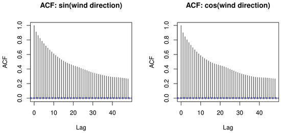
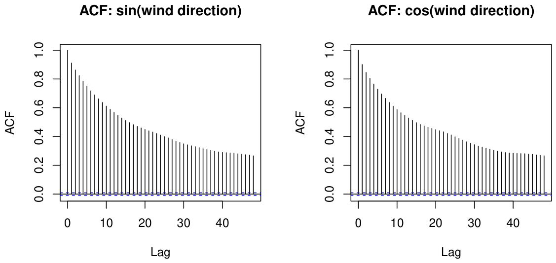
Figure 1 confirms the strength of this temporal dependence directly: the autocorrelation of both sin and cos of wind direction remains substantial even at lags of several hours, decaying only gradually, illustrating why a random train/test split—which would place many temporally adjacent, highly correlated observations across both training and test data—would produce misleadingly optimistic performance estimates.

Figure 1. Autocorrelation of $\sin \left(\mathrm{wind}\mathrm{direction}\right)$ and $\cos \left(\mathrm{wind}\mathrm{direction}\right)$ for the Marylebone dataset, computed on the full hourly series. Both components show substantial, slowly decaying autocorrelation over tens of hours, motivating the rolling-origin cross-validation scheme used in this application rather than a random train/test split.

Table 5 reports the mean angular error, averaged across the nine rolling-origin folds together with its Monte Carlo standard error, for the null model, the projected linear model (CCLM), the projected random forest (CCRF), the circular regression tree of Lang et al. [20] (circtree), and CCBART, alongside the residual correlation $\widehat{\rho }$ and the proportion of held-out test points with resultant length $r\left(x\right)$ below 0.1 for the three independently fit methods (Section 2.4 and Section 2.5). CCBART achieves the lowest mean angular error among the five methods (0.2631), though the margin over CCLM (0.2650), circtree (0.2692), and CCRF (0.2699) is modest, representing a reduction of 79.1% over the null model (1.2610). The residual correlation is small and consistent across all three independently fit methods ($\widehat{\rho }$ between $-0.039$ and $-0.053$), and near-zero-norm instability is negligible throughout (at most 0.1% of test points), indicating only a modest departure from the independence assumption in this application.

Table 5. Mean angular error (MAE_θ, with Monte Carlo standard error) for the CC real-data application to wind direction forecasting at Marylebone, London, evaluated via rolling-origin cross-validation. $\widehat{\rho }$ is the residual correlation between the fitted sine and cosine components (Section 2.5), and $r\left(x\right)<0.1$ is the proportion of held-out test points with resultant length below 0.1 (Section 2.4). Both diagnostics are undefined for the null model and circtree, which do not fit two independent components.

Method	${\mathbf{MAE}}_{\mathsf{\theta }}$	SE	$\widehat{\mathsf{\rho }}$	$\mathit{r}\left(\mathit{x}\right)<0.1$
Null model	1.2610	0.0474	—	—
CCLM	0.2650	0.0168	$-0.039$	0.0%
CCRF	0.2699	0.0158	$-0.050$	0.1%
circtree	0.2692	0.0164	—	—
CCBART	0.2631	0.0163	$-0.053$	0.0%

The residual correlation between the fitted sine and cosine components was small for all three independently fit methods, with $\widehat{\rho }=-0.053$ for CCBART, $\widehat{\rho }=-0.050$ for CCRF, and $\widehat{\rho }=-0.039$ for CCLM (Section 2.5), indicating only a modest departure from the independence assumption in this application, consistent across model classes. The proportion of held-out test points with resultant length $r\left(x\right)$ below 0.1—the region in which the point prediction becomes numerically unstable (Proposition 1)—was negligible for all three methods (0.0% for CCBART and CCLM; 0.1% for CCRF). The empirical coverage of the nominal 90% and 95% posterior credible arcs for CCBART was 88.7% and 92.1%, respectively, with average arc lengths of 1.029 and 1.250 radians (Section 2.7).

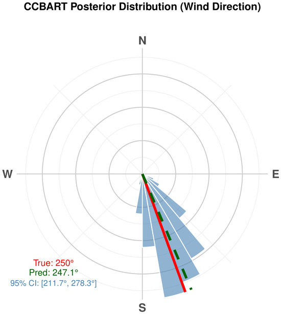
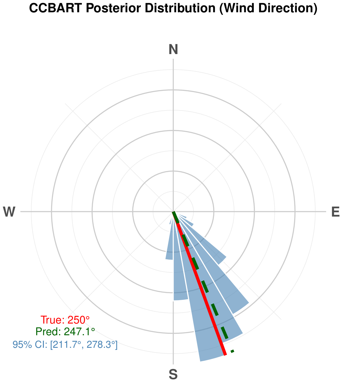
Figure 2 illustrates, for a single representative test observation, the posterior distribution of the predicted wind direction from CCBART, displayed as a circular histogram on a compass rose, using the $\widehat{\Sigma }$-corrected predictive draws described in Section 2.5; this single-observation example is provided as a visual aid only and should not be read as evidence of the method’s uncertainty quantification more broadly. The dataset-wide evidence for CCBART’s uncertainty quantification is instead the empirical coverage and average length of the 90% and 95% posterior credible arcs reported above, computed over all held-out test observations across the rolling-origin folds (Section 2.7). For this observation the 95% credible arc does not cross the $0^{\circ }/{360}^{\circ }$ boundary, but the shortest-arc construction of Section 2.7 is applied uniformly across all test observations regardless of where the interval falls, since which observations wrap is not known in advance and a naive Euclidean interval would misrepresent any boundary-crossing case among the held-out folds.

Figure 2. Posterior distribution of the predicted wind direction from CCBART for a representative test observation, displayed as a circular histogram on a compass rose, using the $\widehat{\Sigma }$-corrected predictive draws described in Section 2.5. The steelblue bars represent the corrected posterior draws, the red line indicates the true wind direction (${250}^{\circ }$), and the green dashed line indicates the posterior mean prediction (${247.1}^{\circ }$). The 95% credible interval, $[{211.7}^{\circ },{278.3}^{\circ }]$, is computed via the shortest-arc construction of Section 2.7, which is applied uniformly regardless of whether a given interval crosses the $0^{\circ }/{360}^{\circ }$ boundary.

4.2. Circular–Linear Case

To illustrate the performance of CLBART on real data, we apply it to hourly wind direction measurements from the Atlantic coast of Galicia, northwest Spain, available in the NPCirc package in R [35]. The dataset speed.wind consists of 19,488 hourly observations recorded between November 2003 and December 2012, containing wind direction (in degrees), wind speed (in metres per second), hour of the day, and month of the year.

4.2.1. Data Description

The response variable is the wind direction (in radians), which is circular. The covariate set consists of three linear variables: wind speed (Speed), month of the year (Month), and hour of the day (Hour). This is a genuine CL regression problem—predicting a circular response from linear covariates.

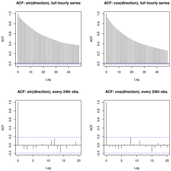
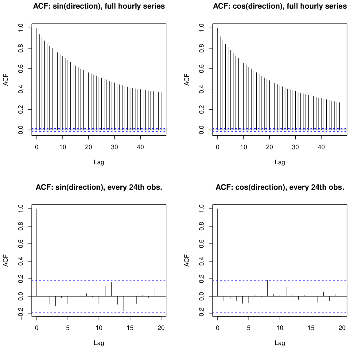
After removing missing values, 19,206 observations remain. To reduce the serial correlation inherent in hourly time series data, every 24th observation is retained, yielding a final sample of 801 observations. We assess this subsampling directly via an autocorrelation diagnostic on the sine and cosine components of wind direction, both before and after subsampling (Figure 3). As in the CC case, we replace a random split with rolling-origin cross-validation, respecting the chronological order of the subsampled series, rather than assuming independence justifies a random split on its own.

Figure 3. Autocorrelation of $\sin \left(\mathrm{wind}\mathrm{direction}\right)$ and $\cos \left(\mathrm{wind}\mathrm{direction}\right)$ for the Galicia dataset, before (top) and after (bottom) retaining every 24th observation.

4.2.2. Results

Unlike the Circular–Circular application (Section 4.1), where lagged wind direction provided strong predictive signal, the covariate set here (wind speed, month, and hour) explains very little of the variation in wind direction. This weak signal is reflected directly in the diagnostics introduced in Section 2.4 and Section 2.5: the residual correlation $\widehat{\rho }$ is substantially larger here (0.399 for CLBART, 0.324 for CLRF, and 0.318 for CLLM) than the near-zero values observed in the Circular–Circular application (Table 5), indicating a more pronounced departure from the independence assumption. Notably, the projected normal regression of Presnell et al. [19] (CLPNR), which fits the two components jointly rather than independently, shows a markedly lower residual correlation ($\widehat{\rho }=0.247$) than any of the independently fit methods—consistent with joint estimation directly accounting for the dependence that the other methods must instead diagnose after the fact. The proportion of held-out test points with resultant length $r\left(x\right)<0.1$ is small in absolute terms (0.0% for CLBART and CLPNR, 6.5% for CLRF, and 2.2% for CLLM) but still notably higher for CLRF and CLLM than anywhere observed in the CC application.

Table 6 reports the mean angular error, averaged across the rolling-origin folds together with its Monte Carlo standard error, for the null model, the projected linear model (CLLM), the projected normal regression of Presnell et al. [19] (CLPNR), the projected random forest (CLRF), the circular regression tree of Lang et al. [20] (circtree), and CLBART. We additionally fit CLPNR, the projected normal regression model of Presnell et al. [19], using spml.reg from the Directional package [33], which jointly estimates the mean vector of the underlying bivariate normal via maximum likelihood, rather than via the two-part independent-OLS approximation to it used by CLLM. CLPNR achieves a mean angular error of 1.4361, an improvement over CLLM (1.4505) consistent with the benefit of joint over independent fitting, though it remains outperformed by CLBART (1.3635). CLBART’s mean angular error is higher than the null model and circtree (both 1.3073), though lower than CLLM and CLPNR, and substantially lower than CLRF (1.6227)—a 4.3% increase over the null model. We report this result as a genuine limitation rather than omit or reframe it: it illustrates a setting in which the proposed diagnostics correctly flag a non-trivial departure from the independence assumption, and where no method, including the proposed one, meaningfully outperforms a naive circular-mean baseline, consistent with the tempered claims of Section 3 regarding when the proposed methods offer an advantage.

Table 6. Mean angular error (MAE_θ, with Monte Carlo standard error) for the CL real-data application to wind direction forecasting at the Atlantic coast of Galicia, Spain, evaluated via rolling-origin cross-validation. $\widehat{\rho }$ is the residual correlation between the fitted sine and cosine components (Section 2.5), and $r\left(x\right)<0.1$ is the proportion of held-out test points with resultant length below 0.1 (Section 2.4). Both diagnostics are undefined for the null model and circtree, which do not fit two independent components.

Method	${\mathbf{MAE}}_{\mathsf{\theta }}$	SE	$\widehat{\mathsf{\rho }}$	$\mathit{r}\left(\mathit{x}\right)<0.1$
Null model	1.3073	0.0665	—	—
CLLM	1.4505	0.0863	$0.318$	2.2%
CLPNR	1.4361	0.0827	$0.247$	0.0%
CLRF	1.6227	0.0927	$0.324$	6.5%
circtree	1.3073	0.0665	—	—
CLBART	1.3635	0.0628	$0.399$	0.0%

Correspondingly, CLBART’s $\widehat{\Sigma }$-corrected credible arcs are very wide: the empirical coverage of the nominal 90% and 95% posterior credible arcs was 77.5% and 86.9%, respectively, with average arc lengths of 4.697 and 5.331 radians (Section 2.7)—both undercovering their nominal levels and close to the maximum possible arc length of $2\pi \approx 6.283$ radians, reflecting the weak predictive signal available in this covariate set and the correspondingly large estimated $\widehat{\Sigma }$.

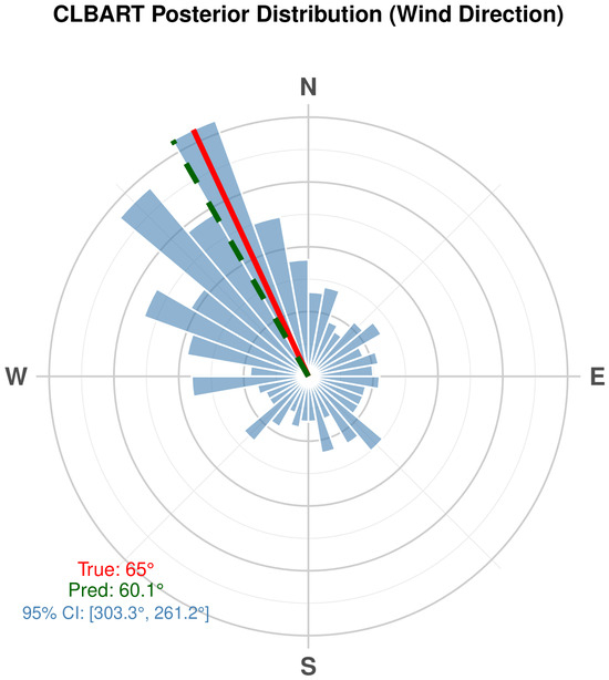
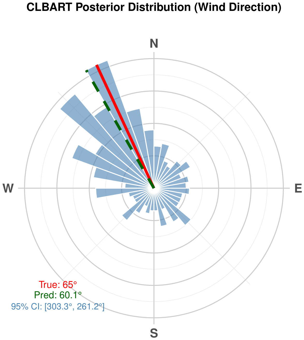
Figure 4 illustrates, for a single representative test observation, the posterior distribution of the predicted wind direction from CLBART, displayed as a circular histogram on a compass rose, using the $\widehat{\Sigma }$-corrected predictive draws described in Section 2.5; as with the CC application, this example is a visual aid rather than the primary evidence for the method’s uncertainty quantification. The dataset-wide evidence is instead the empirical coverage and average arc length reported above (Section 2.7).

Figure 4. Posterior distribution of the predicted wind direction from CLBART for a representative test observation, displayed as a circular histogram on a compass rose, using the $\widehat{\Sigma }$-corrected predictive draws described in Section 2.5. The red line indicates the true wind direction (${65}^{\circ }$), and the green dashed line indicates the posterior mean prediction (${60.1}^{\circ }$). The 95% credible interval, $[{303.3}^{\circ },{261.2}^{\circ }]$, wraps around the $0^{\circ }/{360}^{\circ }$ boundary and spans nearly the entire circle, illustrating the weak predictive signal quantified in Table 6.

4.3. Linear–Circular Case

To illustrate the performance of LCBART on real data, we apply it to the human motor resonance dataset available in the NPCirc package in R [35]. This dataset was originally collected by [36] and consists of 70 observations from a neurophysiology experiment in which participants were asked to observe a rhythmic hand flexion–extension movement performed by a mover. The dataset contains two variables: the angular position of the hand (in radians), which serves as the circular covariate, and the reflex amplitude of the motor resonance response (in microvolts), which is the linear response variable. This is a genuine LC regression problem—predicting a continuous physiological response from a circular covariate—and provides a medically meaningful illustration of LCBART.

4.3.1. Data Description

The circular covariate $\mathrm{\Theta }\in [0,2\pi )$ represents the angular position of the hand at the time of observation, and the linear response y represents the corresponding motor resonance reflex amplitude, which ranges from approximately $-100$ to 150 microvolts. Given the small sample size ($n=63$ after removing missing values), a single train/test split would provide an unstable estimate of predictive performance, and the corresponding test set would contain as few as seven observations. We therefore evaluate all methods using 10-fold cross-validation: the data are partitioned into 10 folds, each method is trained on 9 folds and predicts the held-out fold, and every observation receives exactly one out-of-fold prediction, rotating across all 10 folds.

4.3.2. Results

Table 7 presents the cross-validated RMSE, with Monte Carlo standard error across folds, for the null model, the projected linear model (LCLM), the projected random forest (LCRF), the Nadaraya–Watson and local-linear nonparametric circular-covariate estimators of Di Marzio et al. [37] as implemented in the NPCirc package (NPCirc-NW and NPCirc-LL), and LCBART. The circular regression tree of Lang et al. [20] is not included here, as it is defined only for a circular response via a von Mises likelihood and is not applicable to this linear-response setting. Since LCBART’s response is linear rather than circular, it is fit via a single wbart call rather than two independent components, and the residual correlation and resultant-length diagnostics used elsewhere in the paper for circular responses (Section 2.4 and Section 2.5) do not apply; as a check for remaining unexplained structure, the correlation between held-out residuals and fitted values, pooled across folds, was $-0.171$, indicating no substantial systematic pattern.

Table 7. Cross-validated root mean squared error (RMSE, with Monte Carlo standard error) for the LC real-data application to the human motor resonance dataset, evaluated via 10-fold cross-validation. The null model predicts the training mean for all observations.

Method	RMSE	SE
Null model	45.8394	5.0643
LCLM	37.9019	2.6693
LCRF	41.8709	3.2293
NPCirc-NW	38.2958	3.0813
NPCirc-LL	38.0873	3.0247
LCBART	40.0293	2.8875

All five non-null methods improve substantially over the null model, with cross-validated RMSE reductions ranging from 8.7% (LCRF) to 17.3% (LCLM). LCLM achieves the lowest cross-validated RMSE (37.90), followed by NPCirc-LL (38.09) and NPCirc-NW (38.30); LCBART (40.03) trails these three but improves on LCRF (41.87), yielding a 12.7% reduction over the null model. LCBART is therefore broadly competitive in this application without being the top performer, consistent with the tempered claims made elsewhere in the paper regarding when the proposed methods offer an advantage (Section 3).

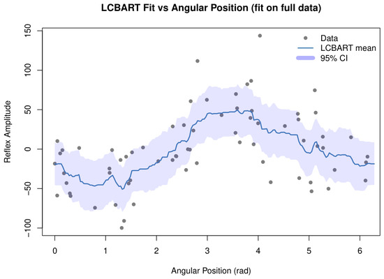
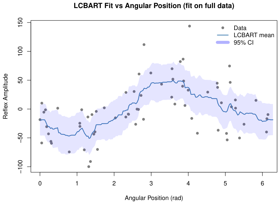
Beyond point prediction, we assess LCBART’s uncertainty quantification directly via genuine prediction intervals, constructed by adding fresh residual noise—drawn using each posterior draw’s own estimated $\sigma$—to the corresponding posterior draw of the mean function, rather than relying on the spread of the mean-function draws alone (which would understate predictive uncertainty). These intervals achieve close to nominal coverage: 92.9% at the 90% level and 94.3% at the 95% level, with average widths of 124.9 and 149.8 microvolts, respectively. Figure 5 illustrates the fitted mean function and 95% credible interval as a function of the circular covariate, fit on the full dataset.

Figure 5. LCBART fitted curve (blue line) and 95% posterior credible interval (shaded blue region) as a function of the circular covariate (hand angular position in radians), fit on the full dataset and overlaid on the data (grey points). This is an illustrative full-data fit rather than a held-out evaluation; the cross-validated performance and prediction-interval coverage reported above (Table 7) constitute the primary evidence for LCBART’s predictive accuracy and uncertainty quantification in this application.

5. Conclusions

In this paper, we have proposed a family of Bayesian Additive Regression Tree (BART) methods for regression with circular data, covering three cases: Circular–Circular BART (CCBART), Circular–Linear BART (CLBART), and Linear–Circular BART (LCBART). The proposed methods adopt a projection approach, decomposing circular variables into their sine and cosine components, fitting separate BART models on these projections, and recovering circular predictions via the two-argument arctangent function $\mathrm{atan2}(·,·)$. This avoids specifying a von Mises or wrapped normal likelihood directly for the circular response, while relying on the flexible Euclidean regression model, with Gaussian errors, that BART uses for the projected sine and cosine components—a distinction discussed in detail in Section 2.4. The approach retains the full inferential power of BART, including posterior uncertainty quantification and automatic variable selection.

The performance of the proposed methods was assessed through an extensive simulation study inspired by the five-dimensional test function of [31], adapted to the circular setting. Across all three cases and all nine combinations of sample size ($n\in \{100,250,500\}$) and noise level ($\sigma \in \{0.5,1,2\}$), the following key findings emerged. First, the linear model benchmarks (CCLM, CLLM, and LCLM) were outperformed by the tree-based methods in the large majority of settings, confirming the general importance of nonparametric methods for capturing the nonlinear signal structure inherent in circular regression. Second, CCBART, CLBART, and LCBART tended to outperform their random forest counterparts (CCRF, CLRF, and LCRF) at high noise levels ($\sigma =2$) across all three cases, consistent with the advantage of BART’s regularization prior when the signal-to-noise ratio is low; this advantage was not uniform, however, and the random forest benchmark outperformed the proposed methods at several low- and moderate-noise CC settings, and, in a single instance, at $n=100$ and $\sigma =0.5$ in the CL case; no such exception occurred in the LC case, where LCBART achieved the lowest RMSE in every setting (Table 1, Table 2 and Table 3). Third, the advantage of LCBART over LCRF was particularly striking in the setting where it held—at $n=500$ and $\sigma =0.5$, LCBART achieved an RMSE of 0.641 compared to 0.966 for LCRF, a reduction of approximately 34%, highlighting that BART’s sum-of-trees structure is especially well-suited to capturing nonlinear relationships between linear responses and circular covariates in higher-signal regimes.

The proposed methods were further illustrated on three real datasets, evaluated via time-aware or standard cross-validation as appropriate (Section 4). For the CC case, CCBART was applied to hourly wind direction data from the Marylebone air quality monitoring supersite in London, achieving a cross-validated mean angular error of 0.2631 radians—a reduction of 79.1% over the circular null model, and outperforming the projected random forest, projected linear model, and circular regression tree benchmarks (Table 5)—by exploiting both the lagged wind direction and atmospheric covariates. For the CL case, CLBART was applied to wind direction data from the Atlantic coast of Galicia, Spain, where the available linear covariates (wind speed, month, and hour) carried very little predictive signal for wind direction; CLBART’s cross-validated mean angular error was 3.7% higher than the circular null model (Table 6), a result we report as a genuine limitation rather than reframe, consistent with the residual-correlation and credible-arc diagnostics (Section 4.2) that correctly flag this as a weak-signal setting. We additionally compared against the projected normal regression of Presnell et al. [19] (CLPNR) in both the simulation study and this real-data application; notably, CLPNR’s advantage over the independently fit CLLM was setting-dependent, improving on CLLM in the real-data application but not in simulation, where the linear predictor common to both methods could not capture the simulation’s nonlinear signal regardless of joint or independent fitting (Section 3 and Section 4.2). We additionally compared against the projected normal regression of Presnell et al. [19] (CLPNR) in both the simulation study and this real-data application; notably, CLPNR’s advantage over the independently fit CLLM was setting-dependent, improving on CLLM in the real-data application but not in simulation, where the linear predictor common to both methods could not capture the simulation’s nonlinear signal regardless of joint or independent fitting (Section 3 and Section 4.2). For the LC case, LCBART was applied to the human motor resonance dataset, capturing a clear nonlinear relationship between hand angular position and reflex amplitude and achieving a 12.7% reduction in cross-validated RMSE over the null model despite only 63 training observations and a single circular covariate, though it was outperformed by three of the four other benchmarks in this application (Table 7). In all three applications, the posterior credible intervals or prediction intervals provided by BART offered meaningful uncertainty quantification for the predictions, which is not available from random forests or linear models.

Having summarized the findings directly supported by the simulation study and real-data applications above, we close by distinguishing these from several promising but as yet unexplored directions suggested by this paper. First, the projection approach adopted here could be extended to more general BART variants, including sparse BART [23] for high-dimensional settings with many irrelevant covariates, soft BART [38] for smoother function estimation, and BART with heteroscedastic errors for settings where the noise variance depends on the covariates. Second, the prior specification for the projected BART models could be tailored more carefully to the circular setting—for example, by imposing joint priors on the sin and cos models that respect the circular geometry of the response, rather than treating them as independent. Third, the projection approach could be extended beyond the circle to higher-dimensional directional data on the sphere ${\mathbb{S}}^2$ or on the torus ${\mathbb{T}}^2={\mathbb{S}}^1\times {\mathbb{S}}^1$, where both response and covariates are directions in three or more dimensions, opening new applications in spatial statistics, geology, and bioinformatics. Finally, while Section 3 demonstrates that posterior inclusion frequencies correctly distinguish relevant from irrelevant covariates in the present simulation design, the development of formal variable-selection procedures with associated inferential guarantees (e.g., thresholding rules with controlled false discovery rates) tailored to circular regression within the BART framework would provide a valuable tool for high-dimensional applications with a larger number of candidate predictors.

References

- Gatto, R.; Jammalamadaka, S.R. Directional Statistics: Introduction. In Wiley StatsRef: Statistics Reference Online; John Wiley & Sons, Ltd.: Hoboken, NJ, USA, 2015; pp. 1–8. [Google Scholar] [CrossRef] [Scilit]
- Ley, C.; Verdebout, T. Modern Directional Statistics; Chapman and Hall/CRC: Boca Raton, FL, USA, 2017. [Google Scholar] [CrossRef] [Scilit]
- Gauss, C.F. Theoria Motus Corporum Coelestium in Sectionibus Conicis Solem Ambientium; Cambridge University Press: Cambridge, UK, 1809. [Google Scholar]
- Langevin, P. Magnétisme et Théorie des Électrons. Ann. Chim. Phys. 1905, 5, 70–127. [Google Scholar]
- Lévy, P. L’addition des variables aléatoires définies sur une circonférence. Bull. Société Mathématique Fr. 1939, 67, 1–41. [Google Scholar] [CrossRef] [Scilit]
- Fisher, R. Dispersion on a Sphere. Proc. R. Soc. A Math. Phys. Eng. Sci. 1953, 217, 295–305. [Google Scholar] [CrossRef] [Scilit]
- Oliveira-Santos, L.; Zucco, C.; Agostinelli, C. Using conditional circular kernel density functions to test hypotheses on animal circadian activity. Anim. Behav. 2013, 85, 269–280. [Google Scholar] [CrossRef] [Scilit]
- Nadarajah, S.; Bell, W. Spatial Modeling of Wind Directions in South Africa. Earth Syst. Environ. 2024, 8, 1477–1501. [Google Scholar] [CrossRef] [Scilit]
- Bell, W.; Nadarajah, S.; Moalafhi, D. Assessing the occurrence of annual maximum daily discharge for five of the longest rivers in Africa. Environ. Ecol. Stat. 2024, 31, 841–863. [Google Scholar] [CrossRef] [Scilit]
- Srivastava, A.N.; Sahami, M. (Eds.) Text Mining: Classification, Clustering, and Applications, 1st ed.; Chapman and Hall/CRC: Boca Raton, FL, USA, 2009. [Google Scholar] [CrossRef] [Scilit]
- Pewsey, A.; García-Portugués, E. Recent advances in directional statistics. Test 2021, 30, 1–58. [Google Scholar] [CrossRef] [Scilit]
- Gould, A.L. A regression technique for angular variates. Biometrics 1969, 25, 683–700. [Google Scholar] [CrossRef] [Scilit]
- Fisher, N.I.; Lee, A.J. Regression models for an angular response. Biometrics 1992, 48, 665–677. [Google Scholar] [CrossRef] [Scilit]
- Sarma, Y.R.; Jammalamadaka, S.R. Circular regression. In Statistical Science and Data Analysis; De Gruyter: Berlin, Germany, 1993; pp. 109–128. [Google Scholar]
- Downs, T.D.; Mardia, K.V. Circular regression. Biometrika 2002, 89, 683–697. [Google Scholar] [CrossRef] [Scilit]
- Kato, S.; Shimizu, K.; Shieh, G.S. A circular–circular regression model. Stat. Sin. 2008, 18, 633–645. [Google Scholar]
- Kim, S.; SenGupta, A. Multivariate–multiple circular regression. J. Stat. Comput. Simul. 2017, 87, 1277–1291. [Google Scholar] [CrossRef] [Scilit]
- Rivest, L.P.; Duchesne, T.; Nicosia, A.; Fortin, D. A general framework for the analysis of animal movement data. Biom. J. 2016, 58, 416–433. [Google Scholar]
- Presnell, B.; Morrison, S.P.; Littell, R.C. Projected multivariate linear models for directional data. J. Am. Stat. Assoc. 1998, 93, 1068–1077. [Google Scholar] [CrossRef]
- Lang, M.N.; Schlosser, L.; Hothorn, T.; Mayr, G.J.; Stauffer, R.; Zeileis, A. Circular regression trees and forests with an application to probabilistic wind direction forecasting. J. R. Stat. Soc. Ser. C Appl. Stat. 2020, 69, 1357–1374. [Google Scholar] [CrossRef] [Scilit]
- Marques F., P.C.; Artes, R.; Graziadei, H. Projected random forests and conformal prediction of circular data. arXiv 2024, arXiv:2410.24145. [Google Scholar]
- Chipman, H.A.; George, E.I.; McCulloch, R.E. BART: Bayesian additive regression trees. Ann. Appl. Stat. 2010, 4, 266–298. [Google Scholar] [CrossRef] [Scilit]
- Linero, A.R. Bayesian regression trees for high-dimensional prediction and variable selection. J. Am. Stat. Assoc. 2018, 113, 626–636. [Google Scholar] [CrossRef] [Scilit]
- Sparapani, R.A.; Logan, B.R.; McCulloch, R.E.; Laud, P.W. Nonparametric survival analysis using Bayesian additive regression trees. Stat. Med. 2016, 35, 2741–2753. [Google Scholar] [CrossRef] [Scilit]
- Hill, J.L. Bayesian nonparametric modeling for causal inference. J. Comput. Graph. Stat. 2011, 20, 217–240. [Google Scholar] [CrossRef] [Scilit]
- Um, S.; Jo, S.; Goo, T.; Sohn, I. Bayesian additive regression trees for multivariate skewed responses. Stat. Med. 2023, 42, 246–263. [Google Scholar] [CrossRef] [Scilit]
- Ročková, V.; Saha, E. On Theory for BART. In Proceedings of the 22nd International Conference on Artificial Intelligence and Statistics (AISTATS); Chaudhuri, K., Sugiyama, M., Eds.; PMLR, Proceedings of Machine Learning Research: Cambridge, MA, USA, 2019; Volume 89, pp. 2839–2848. [Google Scholar]
- Ročková, V.; van der Pas, S. Posterior Concentration for Bayesian Regression Trees and Forests. Ann. Stat. 2020, 48, 2108–2131. [Google Scholar] [CrossRef] [Scilit]
- Wang, F.; Gelfand, A.E. Directional Data Analysis under the General Projected Normal Distribution. Stat. Methodol. 2013, 10, 113–127. [Google Scholar] [CrossRef] [Scilit]
- Breiman, L. Random forests. Mach. Learn. 2001, 45, 5–32. [Google Scholar] [CrossRef] [Scilit]
- Friedman, J.H. Multivariate adaptive regression splines. Ann. Stat. 1991, 19, 1–67. [Google Scholar] [CrossRef] [Scilit]
- Sparapani, R.; Spanbauer, C.; McCulloch, R. Nonparametric Machine Learning and Efficient Computation with Bayesian Additive Regression Trees: The BART R Package. J. Stat. Softw. 2021, 97, 1–66. [Google Scholar] [CrossRef] [Scilit]
- Tsagris, M.; Athineou, G.; Adam, C.; Yu, Z.; Sajib, A.; Amson, E.; Waldstein, M.J.; Papastamoulis, P. Directional: A Collection of Functions for Directional Data Analysis. 2024; R Package. Available online: https://cran.r-project.org/web/packages/Directional/index.html (accessed on 23 August 2026).
- Carslaw, D.C.; Ropkins, K. openair—An R package for air quality data analysis. Environ. Model. Softw. 2012, 27, 52–61. [Google Scholar] [CrossRef] [Scilit]
- Oliveira, M.; Crujeiras, R.M.; Rodríguez-Casal, A. NPCirc: An R package for nonparametric circular methods. J. Stat. Softw. 2014, 61, 1–26. [Google Scholar]
- Puglisi, G.; Leonetti, A.; Landau, A.; Fornia, L.; Cerri, G.; Borroni, P. The role of attention in human motor resonance. PLoS ONE 2017, 12, e0177457. [Google Scholar] [CrossRef] [Scilit]
- Di Marzio, M.; Panzera, A.; Taylor, C.C. Local Polynomial Regression for Circular Predictors. Stat. Probab. Lett. 2009, 79, 2066–2075. [Google Scholar] [CrossRef] [Scilit]
- Linero, A.R.; Yang, Y. Bayesian regression tree ensembles that adapt to smoothness and sparsity. J. R. Stat. Soc. Ser. B Stat. Methodol. 2018, 80, 1087–1110. [Google Scholar] [CrossRef] [Scilit]
Disclaimer/Publisher’s Note: The statements, opinions and data contained in all publications are solely those of the individual author(s) and contributor(s) and not of MDPI and/or the editor(s). MDPI and/or the editor(s) disclaim responsibility for any injury to people or property resulting from any ideas, methods, instructions or products referred to in the content. |
© 2026 by the authors. Licensee MDPI, Basel, Switzerland. This article is an open access article distributed under the terms and conditions of the Creative Commons Attribution (CC BY) license.