A Berry–Esséen Bound for the Edge Frequency Polygon Estimator Under Linearly Extended Negative Quadrant Dependence

Abstract

In this paper, we establish a Berry–Esséen bound for the edge frequency polygon estimator based on linearly extended negative quadrant-dependent (LENQD) random variables under suitable conditions. The convergence rate is shown to be $O\left(n^{-1/6}\right)$, indicating that the edge frequency polygon estimator achieves a convergence performance that is comparable to that of the kernel estimator. In addition, a simulation study is conducted to validate the theoretical findings.

1. Introduction

Density estimation is a fundamental topic in mathematical statistics because it underpins a wide range of nonparametric and semiparametric procedures. The common estimation approaches include histogram estimators, frequency polygon estimators, kernel density estimators, and nearest-neighbor methods. As noted by Scott [1], the frequency polygon estimator possesses a convergence rate that is similar to that of the kernel density estimator and outperforms the histogram estimator. The edge frequency polygon, introduced by Jones et al. [2], provides a piecewise linear alternative to the ordinary frequency polygon.

Let $\left\{X_n,n\ge 1\right\}$ be a sequence of random variables with continuous density function $f\left(x\right)$ on the real line $\mathbb{R}$. Consider a partition $\cdots <x_{-2}<x_{-1}<x_0<x_1<x_2<\cdots$ of $\mathbb{R}$ into equal intervals of length $b_n$, where $b_n\to 0$ as $n\to \infty$. The kth interval is denoted by $I_k=\left[{\displaystyle \frac{(2k-1)b_n}{2}},{\displaystyle \frac{(2k+1)b_n}{2}}\right)$. For any $x\in \mathbb{R}$, there exists some integer $k_0\left(x\right)\stackrel{.}{=}{k}_0$ such that $\left(k_0-{\displaystyle \frac{1}{2}}\right)b_n\le x<\left(k_0+{\displaystyle \frac{1}{2}}\right)b_n$. Consider three adjacent histogram bins $I_{k_{-1}}=\left[\left(k_{-1}-{\displaystyle \frac{1}{2}}\right)b_n,\left(k_{-1}+{\displaystyle \frac{1}{2}}\right)b_n\right)$, $I_{k_0}=\left[\left(k_0-{\displaystyle \frac{1}{2}}\right)b_n,\left(k_0+{\displaystyle \frac{1}{2}}\right)b_n\right)$ and $I_{k_1}=\left[\left(k_1-{\displaystyle \frac{1}{2}}\right)b_n,\left(k_1+{\displaystyle \frac{1}{2}}\right)b_n\right)$, where $k_{-1}=k_0-1$ and $k_1=k_0+1$. Define

$$v_{k_s}={\displaystyle \sum _{i=1}^n}I\left(\left(k_s-{\displaystyle \frac{1}{2}}\right)b_n\le X_i<\left(k_s+{\displaystyle \frac{1}{2}}\right)b_n\right),s=-1,0,1,$$

which count the observations falling into each interval. The corresponding histogram values are denoted by $f_{k_s}=v_{k_s}{\left(n{b}_n\right)}^{-1},s=-1,0,1,$ respectively. The edge frequency polygon estimator ${\widehat{f}}_n\left(x\right)$ of the density function $f\left(x\right)$ is defined as

$${\widehat{f}}_n\left(x\right)=\left({\displaystyle \frac{1}{2}}+k_0-{\displaystyle \frac{x}{b_n}}\right){\displaystyle \frac{f_{k_{-1}}+f_{k_0}}{2}}+\left({\displaystyle \frac{1}{2}}-k_0+{\displaystyle \frac{x}{b_n}}\right){\displaystyle \frac{f_{k_0}+f_{k_1}}{2}},$$

(1)

for $x\in \left[(k_0-{\displaystyle \frac{1}{2}})b_n,(k_0+{\displaystyle \frac{1}{2}})b_n\right).$

The edge frequency polygon retains the simplicity and interpretability of the ordinary frequency polygon with additional theoretical and practical advantages, making it worthy of in-depth investigation.

The frequency polygon estimator ${\tilde{f}}_n\left(x\right)$ of the density function $f\left(x\right)$ is defined as

$$\widetilde{f_n}\left(x\right)=\left({\displaystyle \frac{1}{2}}+k_0-{\displaystyle \frac{x}{b_n}}\right){\overline{f}}_{k_0}+\left({\displaystyle \frac{1}{2}}-k_0+{\displaystyle \frac{x}{b_n}}\right){\overline{f}}_{k_1},$$

(2)

for $x\in \left[(k_0-{\displaystyle \frac{1}{2}})b_n,(k_0+{\displaystyle \frac{1}{2}})b_n\right)$, where ${\overline{f}}_{k_s}={\left(n{b}_n\right)}^{-1}{\displaystyle \sum _{i=1}^n}I\left((k_s-1)b_n\le X_i<k_s{b}_n\right),$ $s=0,1.$

Since the introduction of frequency polygon estimation, many scholars have obtained significant theoretical results. For instance, Carbon et al. [3] proved the asymptotic normality of the frequency polygon for random fields. Yang [4] further investigated the uniformly strong consistency of the frequency polygon for strong mixing samples. Xing et al. [5] proved the uniformly strong consistency of the estimator and obtained a convergence rate. Wen and Xing [6] examined the asymptotic normality of the frequency polygons for $\psi$-mixing samples, and the convergence rate is nearly $O\left(n^{-1/6}\right)$. Xing and Yang [7] extended the uniformly strong consistency of the estimator for negatively associated samples. Xing et al. [8] explored the uniformly strong consistency and Berry–Esséen bound of frequency polygons for $\alpha$-mixing samples. Kang et al. [9] researched the uniformly strong consistency of the estimator for $\psi$-mixing samples. Xi et al. [10] studied the uniformly strong consistency and the convergence rate of asymptotic normality for the edge frequency polygon estimator. Younso [11] examined the strong consistency of the frequency polygon estimators for strongly mixing sequences of real variables. Wu and Wang [12] established the Berry–Esséen bound of the frequency polygon estimation with $\rho$-mixing samples. Additionally, Wang et al. [13] investigated the uniformly complete consistency of the frequency polygon estimation under m-extended negatively dependent (m-END) samples. Chao and Hu [14] obtained the convergence rate of asymptotic normality of the frequency polygon estimator for widely orthant-dependent (WOD) random variables.

Although the asymptotic properties of frequency polygon estimators have been extensively studied under various dependence structures, several important gaps remain. Most existing Berry–Esséen bounds focus on the ordinary frequency polygon, while the edge frequency polygon under more general dependence structures has received much less attention. In particular, the LENQD dependence structure, which includes negatively associated (NA) sequences and is relevant for linear processes and moving average (MA) models, has not yet been considered in this context. The aim of this paper is to fill this gap.

We first recall the definitions of extended negative quadrant-dependent (ENQD) and LENQD sequences, which were introduced by Li et al. [15] as follows.

Definition 1. 

Two random variables X and Y are said to be ENQD if there exists a dominating constant $M\ge 1$ such that, for any $x,y\in \mathbb{R}$,

$$P(X\le x,Y\le y)\le MP(X\le x)P(Y\le y),$$

and

$$P(X>x,Y>y)\le MP(X>x)P(Y>y).$$

A sequence $\{X_n,n\ge 1\}$ is said to be LENQD if, for any disjoint subsets $A,B\subset {\mathbb{Z}}^{+}$ and positive real numbers $\{r_1,r_2,\cdots \}$ or negative real numbers $\{r_1,r_2,\cdots \}$, ${\sum }_{i\in A}{r}_i{X}_i$ and ${\sum }_{j\in B}{r}_j{X}_j$ are ENQD.

Remark 1. 

When $M=1$, ENQD reduces to NQD. LNQD implies LENQD from the definitions, but the converse is not true. Moreover, LENQD is much weaker than the NA dependence structure introduced by Joag-Dev and Proschan [16], as well as NQD and LNQD. Furthermore, extended negatively dependent (END) random variables introduced by Liu [17] are not LENQD, and LENQD random variables are also not END. Hence, the investigation of the limit properties for LENQD random variables is of great interest.

Many interesting theoretical results have been established since the concept of LENQD random variables was introduced by Li et al. [15]. For instance, some probability inequalities were established for LENQD random variables in Li et al. [15], and Li et al. [18] investigated the strong consistency and strong representation for the Kaplan–Meier estimator and hazard rate estimator with censored LENQD data. El Alem [19] presented the Kolmogorov exponential inequality, the Rosenthal-type inequality and the Bernstein-type inequality for m-LENQD random variables. El Alem, Ahra, et al. [20] studied the convergence rate of the central limit theorem for LENQD random variables, among other results.

In this work, we establish the Berry–Esséen bound for the edge frequency polygon estimator based on LENQD samples. The convergence rate is shown to be $O\left(n^{-1/6}\right)$. These results improve the corresponding ones in the existing literature. Moreover, numerical simulations are provided to support the theoretical findings.

The structure of this paper is organized as follows. The main results are presented in Section 2. Section 3 conducts some numerical simulations. Some lemmas and proofs of the main results are listed in Section 4.

Throughout this paper, the symbols $C,C_p$ denote positive constants that are independent of n and may take different values in various positions. Let $\lfloor x\rfloor$ be the integer part of x, $I\left(A\right)$ represents the indicator function of a set A, and $\mathrm{\Phi }\left(u\right)$ is the standard normal distribution function.

2. Basic Assumptions and Main Results

2.1. Basic Assumptions

For the presentation of our main results, the following assumptions are indispensable.

(A1) 

Let $\left\{X,X_n,n\ge 1\right\}$ be a sequence of identically distributed LENQD random variables with a continuous density function $f\left(x\right)\le M$ for $x\in \mathbb{R}$ and some $M>0$. The joint density function $f_{i,j}\left(x,y\right)$ of $\left(X_i,X_j\right)$ exists and satisfies $\underset{\left(x,y\right)\in \mathbb{R}\times \mathbb{R}}{\sup }\left|f_{i,j}\left(x,y\right)-f\left(x\right)f\left(y\right)\right|\le M_1,$ for each $i<j$ and some $M_1>0$.

(A2) 

Set

$${\xi }_{i1,k_s}=I\left\{X_i\ge \left(k_s-1/2\right)b_n\right\}-EI\left\{X_i\ge \left(k_s-1/2\right)b_n\right\},$$

$${\xi }_{i2,k_s}=I\left\{X_i\ge (k_s+1/2)b_n\right\}-EI\left\{X_i\ge (k_s+1/2)b_n\right\},$$

and

$$u\left(q\right)=\underset{j\ge 1}{\sup }\sum _{\left|t-j\right|\ge q}\left|\mathrm{Cov}\left({\xi }_{jl,k_s},{\xi }_{tr,k_s}\right)\right|,\left(l,r=1,2,s=-1,0,1\right).$$

Let $p\stackrel{.}{=}{p}_n$, $q\stackrel{.}{=}{q}_n$ be positive integers tending to ∞. Set ${\sigma }_n^2\left(x\right):=\mathrm{Var}({\widehat{f}}_n\left(x\right))>0$, and there exists some $\delta >0$ such that

$$p+q\le n,q{p}^{-1}\le C<\infty ,$$

and

$${\gamma }_{in}\to 0\left(i=1,2,3\right),u_1\left(q\right)\to 0,\begin{array}{c}\hfill q{b}_n\to 0,\end{array}$$

as $n\to \infty$, where

$$\begin{array}{c}\hfill {\gamma }_{1n}=q/p,{\gamma }_{2n}=p/n,{\gamma }_{3n}={\left[p/\left(n{b}_n\right)\right]}^{\delta /2},u_1\left(q\right)={\left(b_n\right)}^{-1}u\left(q\right).\end{array}$$

Remark 2. 

(i) The assumptions (A1) and (A2) are regular conditions. Similar assumptions have been widely adopted in the literature, such as [7,8,10,11,12,13,14].

(ii) The relationships among the big block size p, the small block size q, the sample size n, and the bin width $b_n$ are established by the Bernstein big-block and small-block procedure. In particular, taking $p=\lfloor n^{3/5}\rfloor$, $q=\lfloor n^{1/6}\rfloor$, $b_n=O\left(n^{-1/5}\right)$, and $u\left(q\right)=O\left(n^{-1/4}\right)$, all the conditions in (A2) can be satisfied.

2.2. Main Results

Now we state our main results. The following result is about the Berry–Esséen bound of the edge frequency polygon estimator for LENQD samples.

Theorem 1. 

Suppose that assumptions (A1) and (A2) are satisfied. Then, for $x\in \mathbb{R}$ with $f\left(x\right)>0,$

$$\underset{-\infty <u<\infty }{\sup }\left|F_n\left(u\right)-\mathrm{\Phi }\left(u\right)\right|\le C\left({\gamma }_{1n}^{1/3}+{\gamma }_{2n}^{1/3}+{\gamma }_{3n}+u_1^{1/3}\left(q\right)\right),$$

(3)

where $F_n\left(u\right)=P\left(S_n\left(x\right)\le u\right)$, $S_n\left(x\right)={\sigma }_n^{-1}\left(x\right)\left[\widehat{f_n}\left(x\right)-E\widehat{f_n}\left(x\right)\right]$.

Corollary 1. 

Suppose that the conditions of Theorem 1 are satisfied. Take $p=\lfloor n^{\rho }\rfloor$, $q=\lfloor n^{2\rho -1}\rfloor$ with $1/2<\rho <3/5$, $b_n=O\left(n^{-1/5}\right)$, $u\left(q\right)=O\left(n^{-\alpha }\right)$ for some $\alpha >1/5$. By choosing $\delta ={\displaystyle \frac{10\left(-1+\rho \right)}{3\left(5\rho -4\right)}}$ and $\alpha ={\displaystyle \frac{6}{5}}-\rho$, we have

$$\underset{-\infty <u<\infty }{\sup }\left|F_n\left(u\right)-\mathrm{\Phi }\left(u\right)\right|=O\left(n^{-{\displaystyle \frac{1-\rho }{3}}}\right).$$

Remark 3. 

(i) The range $1/2<\rho <3/5$ ensures that $q\to \infty$, ${\gamma }_{3n}\to 0$, $\delta >0$, and $q{b}_n\to 0$ simultaneously.

(ii) Since $1/2<\rho <3/5$ and as $\rho \to {\left(1/2\right)}^{+}$, we obtain that the convergence rate is nearly $O\left(n^{-1/6}\right)$. Xing et al. [8] studied the uniformly asymptotic normality of the frequency polygon estimator for α-mixing samples and obtained the convergence rate $O\left(n^{-1/11}\right)$. Wen and Xing [6] derived the convergence rate to be close to $O\left(n^{-1/6}\right)$ under ψ-mixing samples. In Xi et al. [10], the convergence rate of the edge frequency polygon estimator achieved for the Berry–Esséen bound was $O\left(n^{-1/6}\right)$. Chao and Hu [14] presented the convergence rate as approximately $O\left(n^{-1/6}\right)$ for WOD sequences under suitable conditions.

The following results can be obtained under additional assumptions.

Theorem 2. 

Suppose that assumptions (A1) and (A2) are satisfied. If $n{b}_n^3\to 0$ as $n\to \infty$, and $f\left(x\right)$ satisfies the local Lipschitz condition around x with $f\left(x\right)>0$, then

$$\underset{-\infty <u<\infty }{\sup }\left|P\left({\tilde{S}}_n\le u\right)-\mathrm{\Phi }\left(u\right)\right|\le \left({\gamma }_{1n}^{1/3}+{\gamma }_{2n}^{1/3}+{\gamma }_{3n}+u_1^{1/3}\left(q\right)+{\left(n{b}_n^3\right)}^{1/2}\right),$$

(4)

where ${\tilde{S}}_n={\sigma }_n^{-1}\left(x\right)\left[{\widehat{f}}_n\left(x\right)-f\left(x\right)\right]$.

According to Theorem 2, the asymptotic normality and the convergence rate of estimator ${\widehat{f}}_n\left(x\right)$ can be obtained under LENQD samples.

Corollary 2. 

Suppose the conditions of Theorem 2 hold. Let $p=\lfloor n^{\rho }\rfloor$, $q=\lfloor n^{2\rho -1}\rfloor$ with $1/2<\rho <5/9$, $b_n=O\left(n^{-4/9}\right)$, $u\left(q\right)=O\left(n^{-\alpha }\right)$ for some $\alpha >4/9$. By choosing appropriate $\delta ={\displaystyle \frac{6(\rho -1)}{9\rho -5}}$ and $\alpha ={\displaystyle \frac{13}{9}}-\rho$, we obtain

$$\underset{-\infty <u<\infty }{\sup }\left|P\left({\tilde{S}}_n\le u\right)-\mathrm{\Phi }\left(u\right)\right|=O\left(n^{-1/6}\right).$$

Corollary 3. 

Under the assumptions of Theorem 2, we have

$${\tilde{S}}_n\stackrel{D}{⟶}N(0,1)asn\to \infty ,$$

where D denotes the convergence in distribution.

Remark 4. 

(i) For the frequency polygon estimator of the density function $f\left(x\right)$, Ref. [8] obtained the rate $O\left(n^{-1/11}\right)$ of $P\left({\displaystyle \frac{{\tilde{f}}_n\left(x\right)-E{\tilde{f}}_n\left(x\right)}{{\sigma }_n\left(x\right)}}\le u\right)$ under stationary α-mixing samples. Additionally, Ref. [12] studied the results of the convergence of $P\left({\displaystyle \frac{{\tilde{f}}_n\left(x\right)-f\left(x\right)}{{\sigma }_n\left(x\right)}}\le u\right)$ to the standard normal distribution and obtained a better rate $O\left(n^{-1/9}\right)$ with $\rho \left(n\right)=O\left(n^{-4/\phantom{-43}3}\right)$.

(ii) In this paper, our results extend to the edge frequency polygon estimator and establish the asymptotic normality of the distribution function of ${\tilde{S}}_n$ for LENQD samples. Furthermore, we obtain the convergence rate $O\left(n^{-1/6}\right)$ of $P\left({\tilde{S}}_n\le u\right)$ approximating the standard normal distribution.

3. Numerical Simulation

In this section, we perform a simulation to investigate the numerical performance of our main established results. The LENQD sequence is generated by an MA(1) model: $X_t=W_t-\tau W_{t-1}$, where $W_t$ is a Gaussian white noise process with mean $\mu$ and standard deviation $\sigma$. An extensive study of annual temperature values in Basel from 1755 to 1957 was conducted by El Alem, Guessoum et al. [21]. Their results showed that the best MA(1) model, according to the Akaike Information Criterion, is with $\tau =0.9,\mu =0$ and $\sigma =0.7$. We adopt these calibrated parameter values for our simulation study. Therefore the sequence $\{W_n,n\ge 0\}$ consists of i.i.d. random variables with standard normal distributions $N(0,{\sigma }^2)$ by the normality test and autocorrelation test, and $X_n=W_n-\tau W_{n-1}$ is a Gaussian process with the same distribution $N(0,(1+{\tau }^2){\sigma }^2)$. The covariance structure is given by $\mathrm{Cov}(X_i,X_j)=-\tau {\sigma }^2$ if $|i-j|=1,$ and $\mathrm{Cov}(X_i,X_j)=0$ otherwise. A negatively correlated Gaussian sequence $\{X_n,n\ge 1\}$ is an NA sequence and also LENQD, as noted by Joag-Dev and Proschan [16] and Remark 1.

For the purpose of comparing the different estimators, we consider the edge frequency polygon estimator ${\widehat{f}}_n\left(x\right)$, the frequency polygon estimator ${\tilde{f}}_n\left(x\right)$, and the Epanechnikov kernel estimator $K\left(u\right)=0.75(1-u^2)I\left(\right|u|\le 1)$, for which the bandwidth is selected by unbiased cross-validation (UCV). The bandwidth for the edge frequency polygon estimator and the frequency polygon estimator is $b_n=n^{-4/9}$. The evaluation points are $x=0.5,0.75,1.0$, and the sample sizes are $n=200,400,600,800,1000,2000$. We repeat the calculation 1000 times using the R software with a fixed random seed (set.seed(123)) to ensure reproducibility.

As shown in Table 1, for some fixed x and $\tau$, it can be observed that the mean squared error (MSE) of the estimators exhibits a general decreasing trend as n increases. Moreover, the MSE of the estimator ${\widehat{f}}_n\left(x\right)$ is consistently smaller than the corresponding MSE of ${\tilde{f}}_n\left(x\right)$. The Epanechnikov kernel estimator yields the smallest MSE. To quantify the performance gap between the edge frequency polygon and the kernel estimator, we compute the relative efficiency $\mathrm{RE}={\mathrm{MSE}}_{\mathrm{kernel}}/{\mathrm{MSE}}_{\mathrm{edge}}$. As shown in the last column of Table 1, RE exhibits a general decreasing trend as n increases. This indicates that the gap narrows as the sample size increases.

Table 1. The MSE of the three estimators with $\tau =0.9$ and relative efficiency (RE = ${\mathrm{MSE}}_{\mathrm{kernel}}$/${\mathrm{MSE}}_{\mathrm{edge}}$).

x	n	${\widehat{\mathit{f}}}_{\mathit{n}}\left(\mathit{x}\right)$	${\tilde{\mathit{f}}}_{\mathit{n}}\left(\mathit{x}\right)$	Kernel Estimator	RE
0.5	200	0.006871	0.011149	0.003446	0.5015
	400	0.005343	0.007739	0.002348	0.4393
	600	0.004379	0.008265	0.001336	0.3051
	800	0.003374	0.005225	0.001274	0.3774
	1000	0.003222	0.004757	0.001070	0.3319
	2000	0.002227	0.003607	0.000562	0.2525
0.75	200	0.005340	0.007519	0.003062	0.5733
	400	0.004245	0.006591	0.001669	0.3931
	600	0.003125	0.004543	0.001109	0.3548
	800	0.003262	0.006090	0.000996	0.3054
	1000	0.002511	0.003437	0.000824	0.3279
	2000	0.001594	0.002097	0.000473	0.2970
1.0	200	0.005808	0.011258	0.002100	0.3616
	400	0.003614	0.006612	0.001291	0.3572
	600	0.002457	0.003768	0.000936	0.3810
	800	0.002716	0.005352	0.000720	0.2652
	1000	0.002563	0.004876	0.000557	0.2175
	2000	0.001339	0.002270	0.000314	0.2348

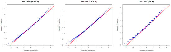
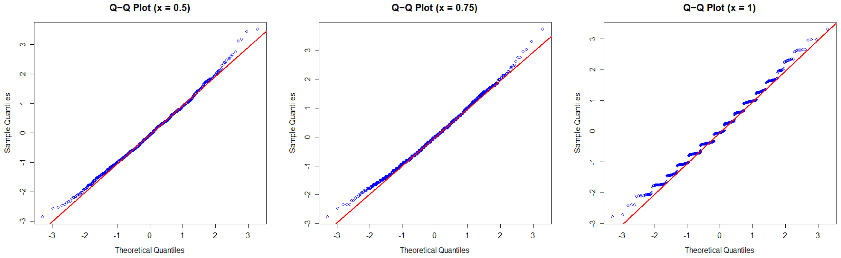
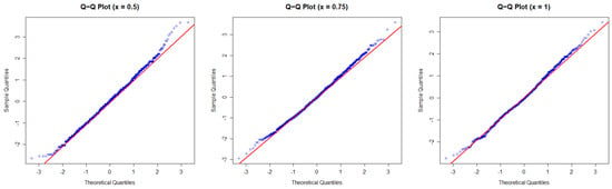
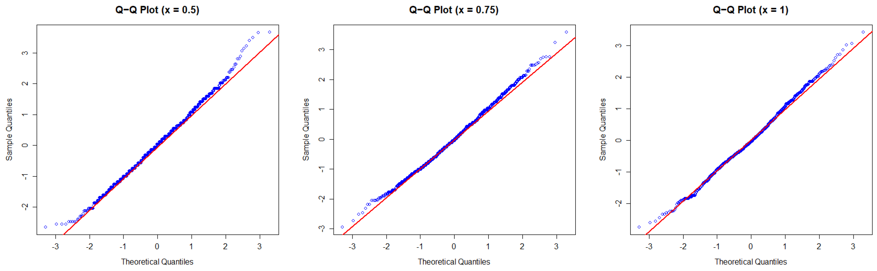
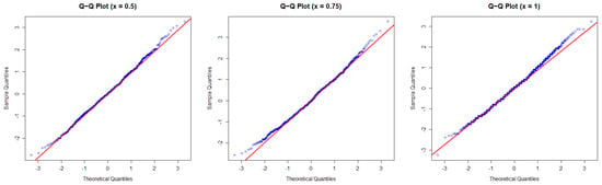
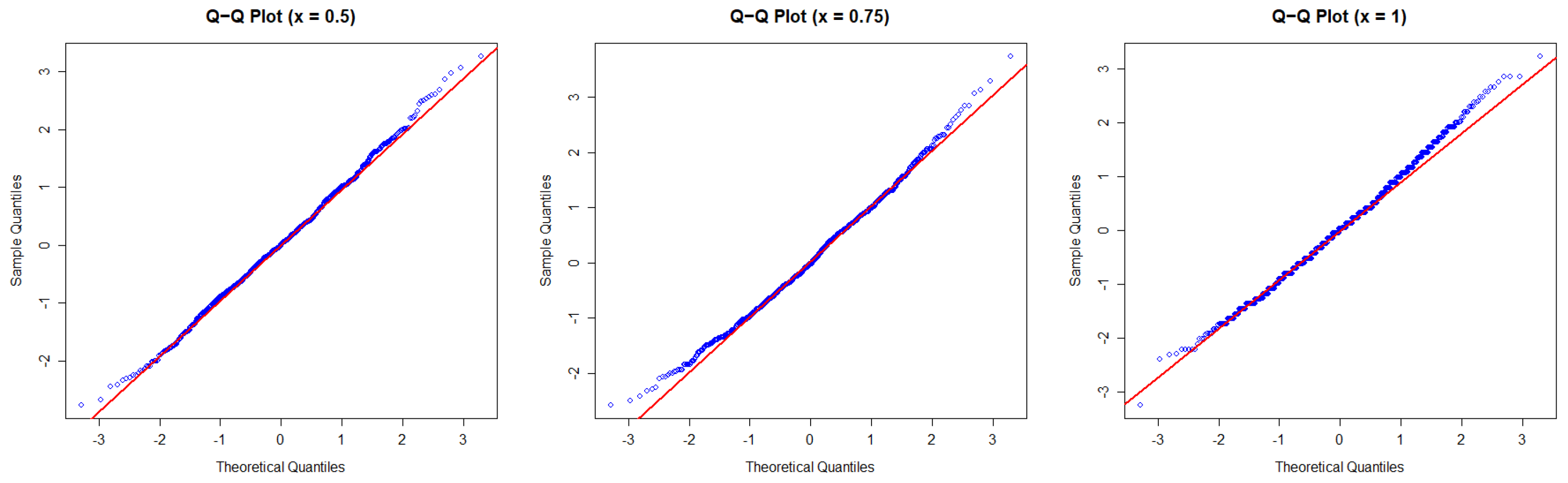
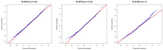
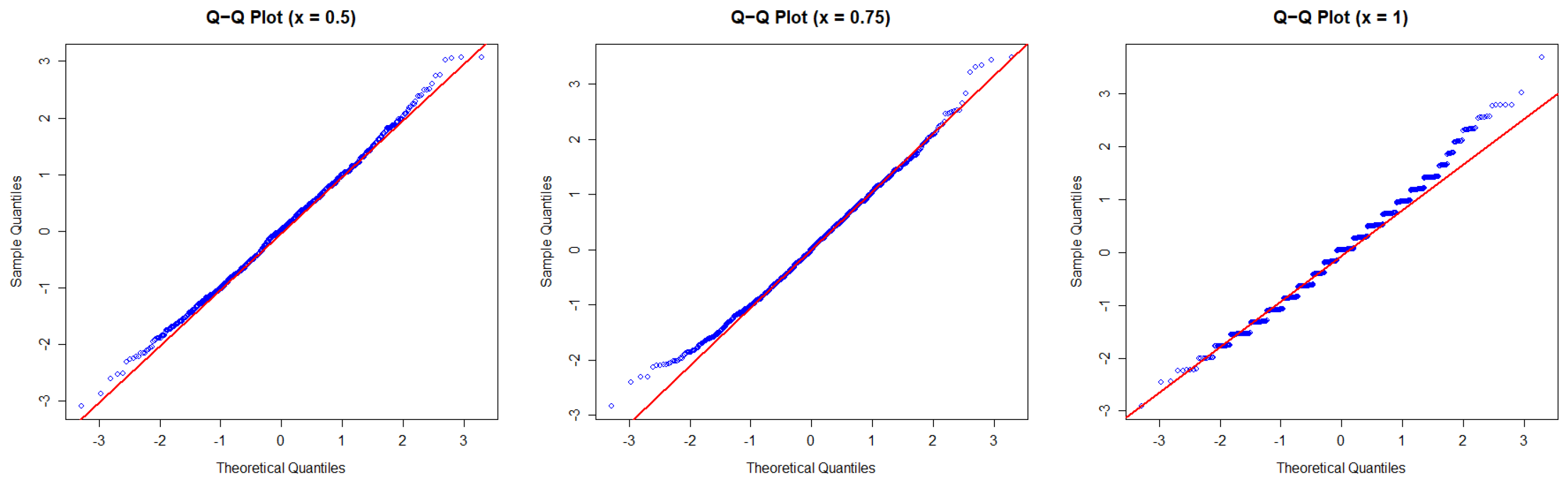
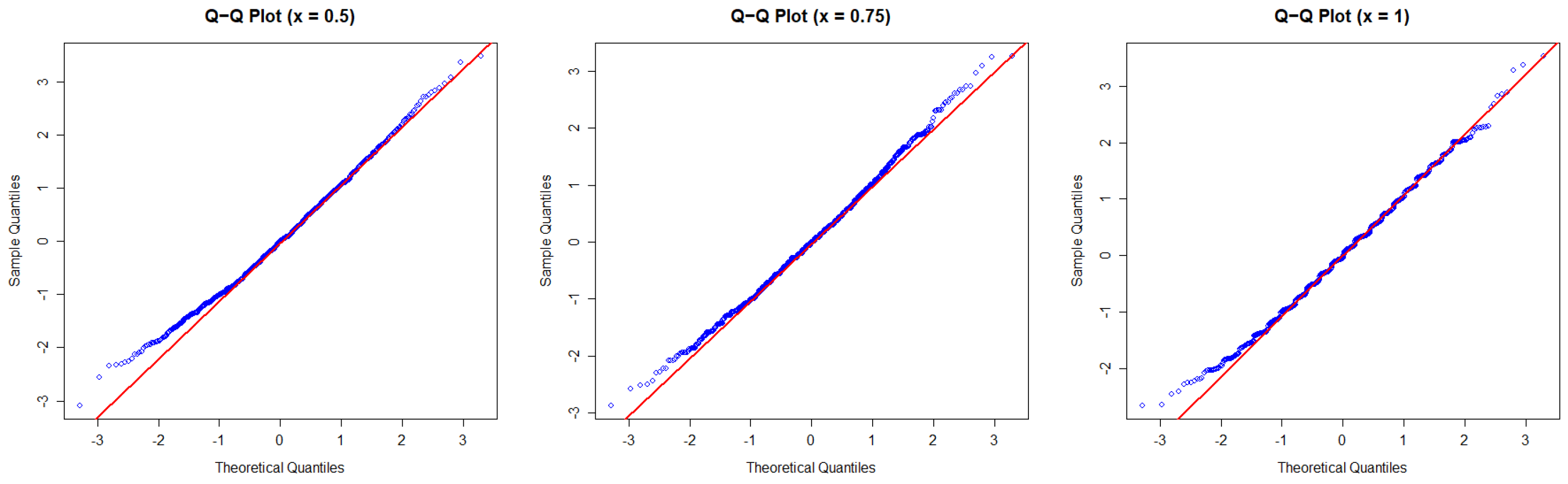
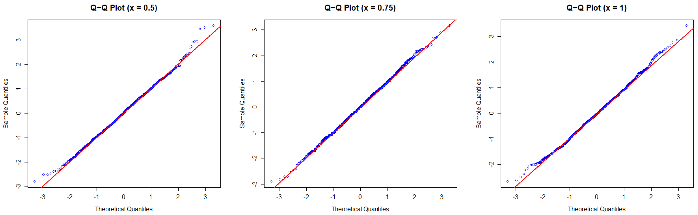
We also construct quantile–quantile (Q–Q) plots of ${\tilde{S}}_n$ to assess its asymptotic normality, as shown in Figure 1, Figure 2, Figure 3, Figure 4, Figure 5 and Figure 6. From these figures, it can be seen that, for each x, ${\tilde{S}}_n$ tends to follow the standard normal distribution.

Figure 1. Q–Q plots of ${\tilde{S}}_n$ with $n=200$ and $x=0.5,0.75,1.0$, respectively.

Figure 2. Q–Q plots of ${\tilde{S}}_n$ with $n=400$ and $x=0.5,0.75,1.0$, respectively.

Figure 3. Q–Q plots of ${\tilde{S}}_n$ with $n=600$ and $x=0.5,0.75,1.0$, respectively.

Figure 4. Q–Q plots of ${\tilde{S}}_n$ with $n=800$ and $x=0.5,0.75,1.0$, respectively.

Figure 5. Q–Q plots of ${\tilde{S}}_n$ with $n=1000$ and $x=0.5,0.75,1.0$, respectively.

Figure 6. Q–Q plots of ${\tilde{S}}_n$ with $n=2000$ and $x=0.5,0.75,1.0$, respectively.

For a quantitative assessment, we compute the Kolmogorov distance,

$$D_n=\underset{-\infty <u<\infty }{\sup }|P({\tilde{S}}_n\le u)-\mathrm{\Phi }\left(u\right)|.$$

The estimated values of $D_n$ are reported in Table 2. In all the configurations, $D_n$ is below $0.06$. These small magnitudes confirm that the empirical distribution of ${\tilde{S}}_n$ is well approximated by the standard normal distribution.

Table 2. Kolmogorov distance.

n	$\mathit{x}=0.5$	$\mathit{x}=0.75$	$\mathit{x}=1.0$
200	0.045981	0.027960	0.058015
400	0.029805	0.024112	0.028339
600	0.031483	0.028432	0.040399
800	0.028994	0.019660	0.051555
1000	0.028733	0.024983	0.027517
2000	0.022827	0.020153	0.028277

To verify the theoretical convergence rate $O\left(n^{-1/6}\right)$, we examine the scaled quantity $n^{1/6}{D}_n$. The results are presented in Table 3. These values range from approximately 0.06 to 0.16 across all the sample sizes and evaluation points, with no systematic increasing or decreasing trend. This provides quantitative support for the Berry–Esséen bound established in Section 2.

Table 3. Scaled Kolmogorov distance $n^{1/6}{D}_n$.

n	$\mathit{x}=0.5$	$\mathit{x}=0.75$	$\mathit{x}=1.0$
200	0.111195	0.067615	0.140296
400	0.080904	0.065450	0.076923
600	0.091432	0.082572	0.117327
800	0.088339	0.059902	0.157079
1000	0.090862	0.079004	0.087015
2000	0.081026	0.071535	0.100371

In summary, the numerical results corroborate our theoretical findings: the edge frequency polygon estimator is consistent and asymptotically normal under LENQD dependence, with a convergence rate $O\left(n^{-1/6}\right)$.

4. Proofs of Main Results

In this section, we will prove the Berry–Esséen bound for the edge frequency polygon estimator based on LENQD samples. For convenient writing, we first provide the following notations. For each $1\le i\le n,s=-1,0,1,$ denote

$$Y_{i,k_s}=I\left\{\left(k_s-1/2\right)b_n\le X_i<(k_s+1/2)b_n\right\},e_{i,k_s}\left(x\right):=Y_{i,k_s}\left(x\right)-E{Y}_{i,k_s}\left(x\right),$$

$${\eta }_i\left(x\right):=\left({\displaystyle \frac{1}{2}}+k_0-{\displaystyle \frac{x}{b_n}}\right){\displaystyle \frac{e_{i,k_{-1}}\left(x\right)+e_{i,k_0}\left(x\right)}{2}}+\left({\displaystyle \frac{1}{2}}-k_0+{\displaystyle \frac{x}{b_n}}\right){\displaystyle \frac{e_{i,k_0}\left(x\right)+e_{i,k_1}\left(x\right)}{2}},$$

$$Z_{ni}:={\left(n{b}_n{\sigma }_n\left(x\right)\right)}^{-1}{\eta }_i\left(x\right),$$

and then

$$S_n={\sigma }_n^{-1}\left(x\right)\left[\widehat{f_n}\left(x\right)-E\widehat{f_n}\left(x\right)\right]={\displaystyle \sum _{i=1}^n}{Z}_{ni}.$$

Let $k:=k_n=⌊n/\phantom{n\left(p+q\right)}\left(p+q\right)⌋$. By employing Bernstein’s big-block and small-block procedures, $S_n$ can be decomposed into

$$S_n=S_n^{\prime }+S_n^{″}+S_n^{‴},$$

(5)

where

$$S_n^{\prime }={\displaystyle \sum _{m=1}^k}{y}_{nm}^{\prime },S_n^{″}={\displaystyle \sum _{m=1}^k}{y}_{nm}^{″},S_n^{‴}=y_{nm}^{‴},$$

and

$$y_{nm}^{\prime }={\displaystyle \sum _{i=k_m}^{k_m+p-1}}{Z}_{ni},y_{nm}^{″}={\displaystyle \sum _{i=l_m}^{l_m+q-1}}{Z}_{ni},y_{nm}^{‴}={\displaystyle \sum _{i=k\left(p+q\right)+1}^n}{Z}_{ni},$$

$$k_m=\left(m-1\right)\left(p+q\right)+1,l_m=\left(m-1\right)\left(p+q\right)+p+1,m=1,2,\cdots ,k.$$

To derive the main results, the following lemmas are indispensable. The first one is a basic property of LENQD random variables, which was presented by Li et al. [15].

Lemma 1. 

Let $\{X_n,n\ge 1\}$ be LENQD random variables and $\{f_n(·),n\ge 1\}$ non-increasing (or non-decreasing) functions. Then random variables $\{f_n\left(X_n\right),n\ge 1\}$ are LENQD with the common dominating constant M.

The following lemma, which can be found in [15], is the Rosenthal-type inequality for LENQD random variables.

Lemma 2. 

Let $\left\{X_n,n\ge 1\right\}$ be a sequence of LENQD random variables with dominating constant M, and assume that $E{X}_n=0$, $E|X_n{|}^p<\infty$ for $p\ge 2$ and all $n\ge 1$. Then there exists a positive constant $C_p$ depending only on p such that

$$E\left({\left|{\displaystyle \sum _{i=1}^n}{X}_i\right|}^p\right)\le C_p\left\{{\displaystyle \sum _{i=1}^n}E{\left|X_i\right|}^p+M{\left({\displaystyle \sum _{i=1}^n}E{\left|X_i\right|}^2\right)}^{p/2}\right\}.$$

(6)

Lemma 3. 

Under assumptions (A1) and (A2), we have

$$\begin{array}{cc}\hfill n{b}_n{\sigma }_n^2\left(x\right)& ={\left({\displaystyle \frac{1}{2}}+k_0-{\displaystyle \frac{x}{b_n}}\right)}^2{\displaystyle \frac{p_{-1}(1-p_{-1})+p_0(1-p_0)-2p_{-1}{p}_0}{4b_n}}\hfill \\ & +{\left({\displaystyle \frac{1}{2}}-k_0+{\displaystyle \frac{x}{b_n}}\right)}^2{\displaystyle \frac{p_0(1-p_0)+p_1(1-p_1)-2p_0{p}_1}{4b_n}}\hfill \\ \hfill & -\left({\displaystyle \frac{1}{2}}+k_0-{\displaystyle \frac{x}{b_n}}\right)\left({\displaystyle \frac{1}{2}}-k_0+{\displaystyle \frac{x}{b_n}}\right){\displaystyle \frac{p_{-1}{p}_0+p_0{p}_1+p_{-1}{p}_1-p_0(1-p_0)}{2b_n}}+o\left(1\right),\hfill \end{array}$$

(7)

where $p_s={\int }_{(k_s-1/2)b_n}^{(k_s+1/2)b_n}f\left(x\right)dx$ for $s=-1,0,1$. Furthermore, if $f\left(x\right)$ is continuous at x, we have

$$\underset{n\to \infty }{\lim \inf } n{b}_n{\sigma }_n^2\left(x\right)\ge {\displaystyle \frac{f\left(x\right)}{4}}.$$

(8)

Proof. 

By definition,

$$\begin{array}{cc}\hfill {\sigma }_n^2\left(x\right)& =E{\left[{\widehat{f}}_n\left(x\right)-E{\widehat{f}}_n\left(x\right)\right]}^2={\displaystyle \frac{1}{{\left(n{b}_n\right)}^2}}E{\left({\displaystyle \sum _{i=1}^n}{\eta }_i\left(x\right)\right)}^2\hfill \\ \hfill & ={\displaystyle \frac{1}{{\left(n{b}_n\right)}^2}}\left({\displaystyle \sum _{i=1}^n}E{\eta }_i^2\left(x\right)\right)+{\displaystyle \frac{2}{{\left(n{b}_n\right)}^2}}\left(\sum _{1\le i<j\le n}E\left[{\eta }_i\left(x\right){\eta }_j\left(x\right)\right]\right)=I_1+I_2.\hfill \end{array}$$

For $I_1$, note that $Y_{i,k_s}{Y}_{i,k_t}=0,k_s\ne k_t,s,t=-1,0,1$ for each $1\le i\le n.$ Therefore, we obtain

$$\begin{array}{cc}\hfill I_1& ={\displaystyle \frac{1}{4{\left(n{b}_n\right)}^2}}\left[{\left({\displaystyle \frac{1}{2}}+k_0-{\displaystyle \frac{x}{b_n}}\right)}^2{\displaystyle \sum _{i=1}^n}E{(e_{i,k_{-1}}\left(x\right)+e_{i,k_0}\left(x\right))}^2\right.\hfill \\ \hfill & +{\left({\displaystyle \frac{1}{2}}-k_0+{\displaystyle \frac{x}{b_n}}\right)}^2{\displaystyle \sum _{i=1}^n}E{(e_{i,k_0}\left(x\right)+e_{i,k_1}\left(x\right))}^2\hfill \\ \hfill & \left.+2\left({\displaystyle \frac{1}{2}}+k_0-{\displaystyle \frac{x}{b_n}}\right)\left({\displaystyle \frac{1}{2}}-k_0+{\displaystyle \frac{x}{b_n}}\right){\displaystyle \sum _{i=1}^n}E(e_{i,k_{-1}}\left(x\right)+e_{i,k_0}\left(x\right))(e_{i,k_0}\left(x\right)+e_{i,k_1}\left(x\right))\right]\hfill \\ \hfill & ={\displaystyle \frac{1}{n{b}_n}}\left[{\left({\displaystyle \frac{1}{2}}+k_0-{\displaystyle \frac{x}{b_n}}\right)}^2{\displaystyle \frac{p_{-1}(1-p_{-1})+p_0(1-p_0)-2p_{-1}{p}_0}{4b_n}}\right.\hfill \\ \hfill & +{\left({\displaystyle \frac{1}{2}}-k_0+{\displaystyle \frac{x}{b_n}}\right)}^2{\displaystyle \frac{p_0(1-p_0)+p_1(1-p_1)-2p_0{p}_1}{4b_n}}\hfill \\ \hfill & \left.-\left({\displaystyle \frac{1}{2}}+k_0-{\displaystyle \frac{x}{b_n}}\right)\left({\displaystyle \frac{1}{2}}-k_0+{\displaystyle \frac{x}{b_n}}\right){\displaystyle \frac{p_{-1}{p}_0+p_0{p}_1+p_{-1}{p}_1-p_0(1-p_0)}{2b_n}}\right].\hfill \end{array}$$

(9)

For $I_2$, we have

$$\begin{array}{cc}\hfill I_2& ={\displaystyle \frac{2}{{\left(n{b}_n\right)}^2}}\sum _{1\le i<j\le n}\left\{\left|{\left({\displaystyle \frac{1}{2}}+k_0-{\displaystyle \frac{x}{b_n}}\right)}^{2}E\left({\displaystyle \frac{e_{i,k_{-1}}\left(x\right)+e_{i,k_0}\left(x\right)}{2}}\right)\left({\displaystyle \frac{e_{j,k_{-1}}\left(x\right)+e_{j,k_0}\left(x\right)}{2}}\right)\right|\right.\hfill \\ \hfill & +\left|{\left({\displaystyle \frac{1}{2}}-k_0+{\displaystyle \frac{x}{b_n}}\right)}^{2}E\left({\displaystyle \frac{e_{i,k_0}\left(x\right)+e_{i,k_1}\left(x\right)}{2}}\right)\left({\displaystyle \frac{e_{j,k_0}\left(x\right)+e_{j,k_1}\left(x\right)}{2}}\right)\right|\hfill \\ \hfill & +\left|\left({\displaystyle \frac{1}{2}}+k_0-{\displaystyle \frac{x}{b_n}}\right)\left({\displaystyle \frac{1}{2}}-k_0+{\displaystyle \frac{x}{b_n}}\right)E\left({\displaystyle \frac{e_{i,k_{-1}}\left(x\right)+e_{i,k_0}\left(x\right)}{2}}\right)\left({\displaystyle \frac{e_{j,k_0}\left(x\right)+e_{j,k_1}\left(x\right)}{2}}\right)\right|\hfill \\ \hfill & \left.+\left|\left({\displaystyle \frac{1}{2}}+k_0-{\displaystyle \frac{x}{b_n}}\right)\left({\displaystyle \frac{1}{2}}-k_0+{\displaystyle \frac{x}{b_n}}\right)E\left({\displaystyle \frac{e_{i,k_0}\left(x\right)+e_{i,k_1}\left(x\right)}{2}}\right)\left({\displaystyle \frac{e_{j,k_{-1}}\left(x\right)+e_{j,k_0}\left(x\right)}{2}}\right)\right|\right\}\hfill \\ \hfill & =J_1+J_2+J_3+J_4.\hfill \end{array}$$

(10)

Next we will prove $J_i=o\left({\left(n{b}_n\right)}^{-1}\right),i=1,2,3,4.$ It follows from (A1) that

$$\begin{array}{cc}\hfill \left|E\left(e_{i,k_s}·e_{j,k_s}\right)\right|& =\left|E\left[\left(Y_{i,k_s}-E{Y}_{i,k_s}\right)\left(Y_{j,k_s}-E{Y}_{j,k_s}\right)\right]\right|\hfill \\ \hfill & =\left|{\int }_{(k_s-1/2)b_n}^{(k_s+1/2)b_n}{\int }_{(k_s-1/2)b_n}^{(k_s+1/2)b_n}f(x,y)dxdy-{\int }_{(k_s-1/2)b_n}^{(k_s+1/2)b_n}f\left(x\right)dx{\int }_{(k_s-1/2)b_n}^{(k_s+1/2)b_n}f\left(y\right)dy\right|\hfill \\ \hfill & \le M_1{b}_n^2.\hfill \end{array}$$

On the other hand, by Lemma 1, it follows that $\left\{{\xi }_{ir,k_s},1\le i\le n\right\}(r=1,2)$ are also LENQD sequences, with $\left|{\xi }_{ir,k_s}\right|\le 2$ and $E{\xi }_{ir,k_s}=0$, combined with assumption (A2), and then we get

$$\begin{array}{cc}\hfill \left|J_1\right|& ={\displaystyle \frac{2}{{\left(n{b}_n\right)}^2}}{\left({\displaystyle \frac{1}{2}}+k_0-{\displaystyle \frac{x}{b_n}}\right)}^2\sum _{1\le i<j\le n}\left|E\left({\displaystyle \frac{e_{i,k_{-1}}\left(x\right)+e_{i,k_0}\left(x\right)}{2}}\right)\left({\displaystyle \frac{e_{j,k_{-1}}\left(x\right)+e_{j,k_0}\left(x\right)}{2}}\right)\right|\hfill \\ \hfill & \le {\displaystyle \frac{2}{{\left(n{b}_n\right)}^2}}{\left({\displaystyle \frac{1}{2}}+k_0-{\displaystyle \frac{x}{b_n}}\right)}^2{\displaystyle \sum _{i=1}^{n-q_n}}\sum _{j-i<q_n}\left|E\left({\displaystyle \frac{e_{i,k_{-1}}\left(x\right)+e_{i,k_0}\left(x\right)}{2}}\right)\left({\displaystyle \frac{e_{j,k_{-1}}\left(x\right)+e_{j,k_0}\left(x\right)}{2}}\right)\right|\hfill \\ \hfill & +{\displaystyle \frac{2}{{\left(n{b}_n\right)}^2}}{\left({\displaystyle \frac{1}{2}}+k_0-{\displaystyle \frac{x}{b_n}}\right)}^2{\displaystyle \sum _{i=1}^n}\sum _{j-i\ge q_n}\left|E\left({\displaystyle \frac{e_{i,k_{-1}}\left(x\right)+e_{i,k_0}\left(x\right)}{2}}\right)\left({\displaystyle \frac{e_{j,k_{-1}}\left(x\right)+e_{j,k_0}\left(x\right)}{2}}\right)\right|\hfill \\ \hfill & \le C{M}_1{\displaystyle \frac{2}{{\left(n{b}_n\right)}^2}}(n-q_n)·\left(q_n\right)b_n^2\hfill \\ \hfill & +{\displaystyle \frac{2}{n{b}_n^2}}\underset{i\ge 1}{\sup }\sum _{\left|j-i\right|\ge q_n}\left|\mathrm{Cov}\left({\displaystyle \frac{{\xi }_{i1,k_{-1}}-{\xi }_{i2,k_{-1}}+{\xi }_{i1,k_0}-{\xi }_{i2,k_0}}{2}},{\displaystyle \frac{{\xi }_{j1,k_{-1}}-{\xi }_{j2,k_{-1}}+{\xi }_{j1,k_0}-{\xi }_{j2,k_0}}{2}}\right)\right|\hfill \\ \hfill & =2C{M}_1{\displaystyle \frac{(n-q_n)·q_n}{n^2}}+{\displaystyle \frac{1}{2n{b}_n^2}}\underset{i\ge 1}{\sup }\sum _{\left|j-i\right|\ge q_n}\sum _{r,l=1,2}\sum _{s,m=-1,0}\left|\mathrm{Cov}\left({\xi }_{ir,k_s},{\xi }_{jl,k_m}\right)\right|\hfill \\ \hfill & =O(q_n/n)+o\left({\left(n{b}_n\right)}^{-1}\right),\hfill \end{array}$$

and, similarly, we can conclude that $\left|J_i\right|=O(q_n/n)+o\left({\left(n{b}_n\right)}^{-1}\right),i=2,3,4.$ Note that $q_n{b}_n\to 0$ as $n\to \infty$, so we obtain $I_2=o\left({\left(n{b}_n\right)}^{-1}\right),$ which, together with (9), yields (7).

Furthermore, if $f(·)$ is continuous at x, then ${\sup }_{(k_{-1}-1/2)b_n\le t<(k_1+1/2)b_n}|t-x|\le 2b_n\to 0$ for any $(k_{-1}-1/2)b_n\le t<(k_1+1/2)b_n, f\left(t\right)=f\left(x\right)+o\left(1\right)$. Therefore, we have for $s=-1,0,1$ that

$$p_s={\int }_{(k_s-1/2)b_n}^{(k_s+1/2)b_n}f\left(x\right)dx=(f\left(x\right)+o\left(1\right))b_n.$$

This is similar to the proof of Lemma 4.1 in [12], which, combined with (7), yields (8). The proof of Lemma 3 is completed. □

Lemma 4. 

Suppose that assumptions (A1) and (A2) hold; we have

$$E{\left(S_n^{″}\right)}^2\le C{\gamma }_{1n},E{\left(S_n^{‴}\right)}^2\le C{\gamma }_{2n}.$$

(11)

Proof. 

According to $C_r$ inequality, Jensen’s inequality and $f\left(x\right)\le M$, for any $r>1$, it follows that

$$\begin{array}{cc}\hfill \underset{1\le i\le n}{\max }E{\left|{\eta }_i\left(x\right)\right|}^r& \le 2^{r-1}\underset{1\le i\le n}{\max }E{\left|{\displaystyle \frac{e_{i,k_{-1}}\left(x\right)+e_{i,k_0}\left(x\right)}{2}}\right|}^r+2^{r-1}\underset{1\le i\le n}{\max }E{\left|{\displaystyle \frac{e_{i,k_1}\left(x\right)+e_{i,k_0}\left(x\right)}{2}}\right|}^r\hfill \\ \hfill & \le C\left({\int }_{\left(k_{-1}-1/2\right)b_n}^{\left(k_{-1}+1/2\right)b_n}f\left(t\right)dt+{\int }_{\left(k_0-1/2\right)b_n}^{\left(k_0+1/2\right)b_n}f\left(t\right)dt+{\int }_{\left(k_1-1/2\right)b_n}^{\left(k_1+1/2\right)b_n}f\left(t\right)dt\right)\hfill \\ \hfill & \le CM{b}_n,\hfill \end{array}$$

and then we can deduce that

$$E{\left|{\eta }_i\left(x\right)\right|}^2\le C{b}_n,E{Z}_{ni}^2=E{\left|{\left(n{b}_n{\sigma }_n\left(x\right)\right)}^{-1}{\eta }_i\left(x\right)\right|}^2\le {\displaystyle \frac{C}{n^2{b}_n{\sigma }_n^2\left(x\right)}}.$$

For a given $k_s,s=-1,0,1$ and $i=1,2,\cdots ,n$, set

$$\begin{array}{cc}\hfill e_{i,k_s}& =I\left\{X_i\ge \left(k_s-1/2\right)b_n\right\}-EI\left\{X_i\ge \left(k_s-1/2\right)b_n\right\}\hfill \\ \hfill & -\left\{I\left\{X_i\ge (k_s+1/2)b_n\right\}-EI\left\{X_i\ge (k_s+1/2)b_n\right\}\right\}\hfill \\ \hfill & :={\xi }_{i1,k_s}-{\xi }_{i2,k_s},\hfill \end{array}$$

and, by Lemma 1, it follows that $\left\{{\xi }_{ir,k_s},1\le i\le n\right\}(r=1,2)$ are LENQD sequences, so the sequence $\{{\eta }_i,i\ge 1\}$ is also LENQD. By Lemmas 2 and 3, we can obtain that

$$\begin{array}{cc}\hfill E{\left(S_n^{″}\right)}^2& =E{\left({\displaystyle \sum _{m=1}^k}{y}_{nm}^{″}\right)}^2=E{\left({\displaystyle \sum _{m=1}^k}{\displaystyle \sum _{i=l_m}^{l_m+q-1}}{Z}_{ni}\right)}^2\hfill \\ \hfill & \le C{\displaystyle \sum _{m=1}^k}{\displaystyle \sum _{i=l_m}^{l_m+q-1}}{\displaystyle \frac{1}{n^2{b}_n{\sigma }_n^2\left(x\right)}}\le C{\displaystyle \frac{kq}{n^2{b}_n{\sigma }_n^2\left(x\right)}}\hfill \\ \hfill & \le C{\displaystyle \frac{n}{p+q}}{\displaystyle \frac{q}{n^2{b}_n{\sigma }_n^2\left(x\right)}}\hfill \\ \hfill & \le C{\displaystyle \frac{q}{p+q}}{\left(n{b}_n{\sigma }_n^2\left(x\right)\right)}^{-1}\le C{\gamma }_{1n},\hfill \end{array}$$

and that

$$\begin{array}{cc}\hfill E{\left(S_n^{‴}\right)}^2& =E{\left(y_{nm}^{‴}\right)}^2=E{\left({\displaystyle \sum _{i=k(p+q)+1}^n}{Z}_{ni}\right)}^2\hfill \\ \hfill & \le C{\displaystyle \sum _{i=k(p+q)+1}^n}{\displaystyle \frac{1}{{\left(n{b}_n^{1/2}{\sigma }_n\left(x\right)\right)}^2}}\hfill \\ \hfill & \le C\left[n-k(p+q)\right]{\displaystyle \frac{1}{{\left(n{b}_n^{1/2}{\sigma }_n\left(x\right)\right)}^2}}\hfill \\ \hfill & \le C{\displaystyle \frac{p}{n^2{b}_n{\sigma }_n^2\left(x\right)}}\le C{\gamma }_{2n}.\hfill \end{array}$$

Hence, (11) holds, and we get by Markov’s inequality that

$$P\left(\left|S_n^{″}\right|\ge {\gamma }_{1n}^{1/3}\right)\le C{\gamma }_{1n}^{1/3},P\left(\left|S_n^{‴}\right|\ge {\gamma }_{2n}^{1/3}\right)\le C{\gamma }_{2n}^{1/3}.$$

(12)

□

Lemma 5. 

Denote $s_n^2={\displaystyle \sum _{m=1}^k}\mathrm{Var}\left(y_{nm}^{\prime }\right).$ Suppose that the assumptions of Theorem 1 are satisfied. We have

$$\left|s_n^2-1\right|\le C\left({\gamma }_{1n}^{1/2}+{\gamma }_{2n}^{1/2}+u_1\left(q\right)\right),$$

(13)

Proof. 

Set ${\mathrm{\Gamma }}_n={\displaystyle \sum _{1\le i<j\le k}}\mathrm{Cov}\left(y_{ni}^{\prime },y_{nj}^{\prime }\right)$. Then, we have

$$s_n^2=E{\left(S_n^{\prime }\right)}^2-2{\mathrm{\Gamma }}_n.$$

(14)

Since $E{\left(S_n\right)}^2=1$, we have

$$E{\left(S_n^{\prime }\right)}^2=1-2E\left[S_n\left(S_n^{″}+S_n^{‴}\right)\right]+E{\left(S_n^{″}+S_n^{‴}\right)}^2,$$

and, combined with $C_r$ inequality and (11), we can obtain that

$$\begin{array}{cc}\hfill \left|E{\left(S_n^{\prime }\right)}^2-1\right|& \le 2E{\left(S_n^{″}\right)}^2+2E{\left(S_n^{‴}\right)}^2+2{\left[E\left(S_n^2\right)\right]}^{1/2}{\left[E{\left(S_n^{″}\right)}^2\right]}^{1/2}\hfill \\ \hfill & +2{\left[E\left(S_n^2\right)\right]}^{1/2}{\left[E{\left(S_n^{‴}\right)}^2\right]}^{1/2}\hfill \\ \hfill & \le 2({\gamma }_{1n}+{\gamma }_{2n})+2{\gamma }_{1n}^{1/2}+2{\gamma }_{2n}^{1/2}\hfill \\ \hfill & \le C({\gamma }_{1n}^{1/2}+{\gamma }_{2n}^{1/2}).\hfill \end{array}$$

(15)

On the other hand, it follows that

$$\begin{array}{cc}\hfill \left|{\mathrm{\Gamma }}_n\right|& \le \sum _{1\le i<j\le k}\left|\mathrm{Cov}\left(y_{ni}^{\prime },y_{nj}^{\prime }\right)\right|\hfill \\ \hfill & \le \sum _{1\le i<j\le k}{\displaystyle \sum _{s=k_i}^{k_i+p-1}}{\displaystyle \sum _{t=k_j}^{k_j+p-1}}\left|\mathrm{Cov}\left(Z_{ns},Z_{nt}\right)\right|\hfill \\ \hfill & \le \sum _{1\le i<j\le k}{\displaystyle \sum _{s=k_i}^{k_i+p-1}}{\displaystyle \sum _{t=k_j}^{k_j+p-1}}{\displaystyle \frac{1}{{\left(n{b}_n{\sigma }_n\left(x\right)\right)}^2}}\left|\mathrm{Cov}\left({\eta }_s,{\eta }_t\right)\right|\hfill \\ \hfill & \le C{\left(n{b}_n{\sigma }_n\left(x\right)\right)}^{-2}{\displaystyle \sum _{i=1}^{k-1}}{\displaystyle \sum _{s=k_i}^{k_i+p-1}}\underset{j\ge 1}{\sup }\sum _{\left|t-j\right|\ge q}\left|\mathrm{Cov}\left({\eta }_j,{\eta }_t\right)\right|\hfill \\ \hfill & \le C{\left({\sigma }_n\left(x\right)\right)}^{-2}{\displaystyle \sum _{i=1}^{k-1}}{\displaystyle \sum _{s=k_i}^{k_i+p-1}}\underset{j\ge 1}{\sup }\sum _{\left|t-j\right|\ge q}{\displaystyle \frac{1}{n^2{b}_n^2}}\hfill \\ \hfill & \times \left\{\left|{\left({\displaystyle \frac{1}{2}}+k_0-{\displaystyle \frac{x}{b_n}}\right)}^2\mathrm{Cov}\left({\displaystyle \frac{e_{j,k_{-1}}\left(x\right)+e_{j,k_0}\left(x\right)}{2}},{\displaystyle \frac{e_{t,k_{-1}}\left(x\right)+e_{t,k_0}\left(x\right)}{2}}\right)\right|\right.\hfill \\ \hfill & +\left|{\left({\displaystyle \frac{1}{2}}-k_0+{\displaystyle \frac{x}{b_n}}\right)}^2\mathrm{Cov}\left({\displaystyle \frac{e_{j,k_0}\left(x\right)+e_{j,k_1}\left(x\right)}{2}},{\displaystyle \frac{e_{t,k_0}\left(x\right)+e_{t,k_1}\left(x\right)}{2}}\right)\right|\hfill \\ \hfill & +\left|\left({\displaystyle \frac{1}{2}}+k_0-{\displaystyle \frac{x}{b_n}}\right)\left({\displaystyle \frac{1}{2}}-k_0+{\displaystyle \frac{x}{b_n}}\right)\mathrm{Cov}\left({\displaystyle \frac{e_{j,k_{-1}}\left(x\right)+e_{j,k_0}\left(x\right)}{2}},{\displaystyle \frac{e_{t,k_0}\left(x\right)+e_{t,k_1}\left(x\right)}{2}}\right)\right|\hfill \\ \hfill & \left.+\left|\left({\displaystyle \frac{1}{2}}+k_0-{\displaystyle \frac{x}{b_n}}\right)\left({\displaystyle \frac{1}{2}}-k_0+{\displaystyle \frac{x}{b_n}}\right)\mathrm{Cov}\left({\displaystyle \frac{e_{j,k_0}\left(x\right)+e_{j,k_1}\left(x\right)}{2}},{\displaystyle \frac{e_{t,k_{-1}}\left(x\right)+e_{t,k_0}\left(x\right)}{2}}\right)\right|\right\}\hfill \\ \hfill & \le C{\left({\sigma }_n\left(x\right)\right)}^{-2}{\displaystyle \sum _{i=1}^{k-1}}{\displaystyle \sum _{s=k_i}^{k_i+p-1}}\left\{\left|Z_{1n}\right|+\left|Z_{2n}\right|+\left|Z_{3n}\right|+\left|Z_{4n}\right|\right\},\hfill \end{array}$$

where

$$Z_{1n}={\displaystyle \frac{1}{n^2{b}_n^2}}\underset{j\ge 1}{\sup }\sum _{\left|t-j\right|\ge q}\mathrm{Cov}\left({\displaystyle \frac{e_{j,k_{-1}}\left(x\right)+e_{j,k_0}\left(x\right)}{2}},{\displaystyle \frac{e_{t,k_{-1}}\left(x\right)+e_{t,k_0}\left(x\right)}{2}}\right),$$

$$Z_{2n}={\displaystyle \frac{1}{n^2{b}_n^2}}\underset{j\ge 1}{\sup }\sum _{\left|t-j\right|\ge q}\mathrm{Cov}\left({\displaystyle \frac{e_{j,k_0}\left(x\right)+e_{j,k_1}\left(x\right)}{2}},{\displaystyle \frac{e_{t,k_0}\left(x\right)+e_{t,k_1}\left(x\right)}{2}}\right),$$

$$Z_{3n}={\displaystyle \frac{1}{n^2{b}_n^2}}\underset{j\ge 1}{\sup }\sum _{\left|t-j\right|\ge q}\mathrm{Cov}\left({\displaystyle \frac{e_{j,k_{-1}}\left(x\right)+e_{j,k_0}\left(x\right)}{2}},{\displaystyle \frac{e_{t,k_0}\left(x\right)+e_{t,k_1}\left(x\right)}{2}}\right),$$

$$Z_{4n}={\displaystyle \frac{1}{n^2{b}_n^2}}\underset{j\ge 1}{\sup }\sum _{\left|t-j\right|\ge q}\mathrm{Cov}\left({\displaystyle \frac{e_{j,k_0}\left(x\right)+e_{j,k_1}\left(x\right)}{2}},{\displaystyle \frac{e_{t,k_{-1}}\left(x\right)+e_{t,k_0}\left(x\right)}{2}}\right).$$

By Lemma 1, it follows that $\left\{{\xi }_{ir,k_s},1\le i\le n\right\}(r=1,2)$ are also LENQD sequences, with $\left|{\xi }_{ir,k_s}\right|\le 2$ and $E{\xi }_{ir,k_s}=0$, combined with assumption (A2), and then we get the following upper bound:

$$\begin{array}{cc}\hfill \left|Z_{1n}\right|& ={\displaystyle \frac{1}{n^2{b}_n^2}}\underset{j\ge 1}{\sup }\sum _{\left|t-j\right|\ge q}\left|\mathrm{Cov}\left({\displaystyle \frac{{\xi }_{j1,k_{-1}}-{\xi }_{j2,k_{-1}}+{\xi }_{j1,k_0}-{\xi }_{j2,k_0}}{2}},{\displaystyle \frac{{\xi }_{t1,k_{-1}}-{\xi }_{t2,k_{-1}}+{\xi }_{t1,k_0}-{\xi }_{t2,k_0}}{2}}\right)\right|\hfill \\ \hfill & ={\displaystyle \frac{1}{4n^2{b}_n^2}}\underset{j\ge 1}{\sup }\sum _{\left|t-j\right|\ge q}\sum _{r,l=1,2}\sum _{s,m=-1,0}\left|\mathrm{Cov}\left({\xi }_{jr,k_s},{\xi }_{tl,k_m}\right)\right|\hfill \\ \hfill & \le C{\displaystyle \frac{u\left(q\right)}{n^2{b}_n^2}},\hfill \end{array}$$

and we can similarly conclude that $\left|Z_{in}\right|\le C{\displaystyle \frac{u\left(q\right)}{n^2{b}_n^2}},i=2,3,4.$

Hence, by Lemma 3, it can be deduced that

$$\left|{\mathrm{\Gamma }}_n\right|\le C{\left(n{b}_n{\sigma }_n\left(x\right)\right)}^{-2}kpu\left(q\right)\le C{u}_1\left(q\right),$$

(16)

combined with (14), (15) and (16). The proof is completed. □

Assume that $\left\{{\eta }_{nm},1\le m\le k\right\}$ are independent random variables and the distribution of ${\eta }_{nm}$ is the same as that of $y_{nm}^{\prime }$ for each $m=1,2,\cdots ,k.$ We define $T_n={\displaystyle \sum _{m=1}^k}{\eta }_{nm}$, $B_n={\displaystyle \sum _{m=1}^k}\mathrm{Var}\left({\eta }_{nm}\right)$, and let ${\tilde{F}}_n\left(u\right)$, $G_n\left(u\right)$ and ${\tilde{G}}_n\left(u\right)$ be the distributions of $S_n^{\prime }$, ${\displaystyle \frac{T_n}{\sqrt{B_n}}}$ and $T_n$, respectively.

Lemma 6. 

Under the assumptions of Theorem 1, we get

$$\underset{u}{\sup }\left|G_n\left(u\right)-\mathrm{\Phi }\left(u\right)\right|\le C{\gamma }_{3n}.$$

Proof. 

Note that $\left|Z_{ni}\right|\le {\displaystyle \frac{e_{i,k_{-1}}\left(x\right)+2e_{i,k_0}\left(x\right)+e_{i,k_1}\left(x\right)}{2n{b}_n{\sigma }_n\left(x\right)}}$. By Lemma 2 and $f\left(x\right)\le M$, for some $\delta >0$, we obtain that

$$\begin{array}{cc}\hfill & {\displaystyle \sum _{m=1}^k}E{\left|{\eta }_{nm}\right|}^{2+\delta }\hfill \\ \hfill & \le C\left\{{\displaystyle \sum _{m=1}^k}{\displaystyle \sum _{i=k_m}^{k_m+p-1}}E{\left|Z_{ni}\right|}^{2+\delta }+{\displaystyle \sum _{m=1}^k}{\left({\displaystyle \sum _{i=k_m}^{k_m+p-1}}E{Z}_{ni}^2\left(x\right)\right)}^{1+\delta /\phantom{\delta 2}2}\right\}\hfill \\ \hfill & \le C\left\{{\displaystyle \frac{pk{b}_n}{{\left(n{b}_n{\sigma }_n\left(x\right)\right)}^{2+\delta }}}+k{\left({\displaystyle \frac{p{b}_n}{{\left(n{b}_n{\sigma }_n\left(x\right)\right)}^2}}\right)}^{1+\delta /\phantom{\delta 2}2}\right\}\hfill \\ \hfill & \le Ck{b}_n{\left\{{\displaystyle \frac{p}{{\left(n{b}_n{\sigma }_n\left(x\right)\right)}^2}}\right\}}^{1+\delta /\phantom{\delta 2}2}\hfill \\ \hfill & \le C{\displaystyle \frac{p^{1+\delta /\phantom{\delta 2}2}{b}_n}{p+q}}\left({\displaystyle \frac{1}{n^{1+\delta }{\left(b_n{\sigma }_n\left(x\right)\right)}^{2+\delta }}}\right)\hfill \\ \hfill & \le C{\displaystyle \frac{p^{\delta /\phantom{\delta 2}2}}{{\left(n{b}_n\right)}^{1+\delta }{\left({\sigma }_n\left(x\right)\right)}^{2+\delta }}}\le C{\gamma }_{3n}.\hfill \end{array}$$

Furthermore, it follows from Lemma 5 that $B_n=s_n^2\to 1$ as $n\to \infty$. Applying the Berry–Esséen theorem (see [22], Theorem 5.7), for $\delta >0$, we get that

$$\underset{u}{\sup }\left|G_n\left(u\right)-\mathrm{\Phi }\left(u\right)\right|\le C{\displaystyle \frac{1}{B_n^{1+\delta /\phantom{\delta 2}2}}}{\displaystyle \sum _{m=1}^k}E{\left|{\eta }_{nm}\right|}^{2+\delta }\le C{\gamma }_{3n}.$$

The proof of Lemma 6 is completed. □

The following lemma was presented in [15].

Lemma 7. 

Let $\left\{X_n,n\ge 1\right\}$ be a sequence of LENQD random variables with dominating constant $M\ge 1$ and with finite second moments. Then, for any finite real numbers $r_j$, $j=1,\cdots ,n,$

$$\left|E\exp \left(\mathrm{i}{\displaystyle \sum _{j=1}^n}{r}_j{X}_j\right)-{\displaystyle \prod _{j=1}^n}E\exp \left(\mathrm{i}{r}_j{X}_j\right)\right|\le 2{\displaystyle \sum _{\begin{array}{c}j\ne l\\ j,l=1\end{array}}^n}\left|r_j{r}_l\mathrm{Cov}\left(X_{j,}{X}_l\right)\right|.$$

Lemma 8. 

Under the conditions of Theorem 1, we have

$$\underset{u}{\sup }\left|{\tilde{F}}_n\left(u\right)-{\tilde{G}}_n\left(u\right)\right|\le C\left({\gamma }_{3n}+u_1^{1/3}\left(q\right)\right).$$

Proof. 

Let $\phi \left(t\right)$ and $\psi \left(t\right)$ be the characteristic functions of $S_n^{\prime }$ and $T_n$, respectively. By Berry–Esséen inequality (see [22], Theorem 5.3), we have for any $T>0$ that

$$\begin{array}{cc}\hfill \underset{u}{\sup }\left|{\tilde{F}}_n\left(u\right)-{\tilde{G}}_n\left(u\right)\right|& \le {\int }_{-T}^T\left|{\displaystyle \frac{\phi \left(t\right)-\psi \left(t\right)}{t}}\right|dt+T\underset{u}{\sup }{\int }_{\left|y\right|\le c/\phantom{cT}T}\left|{\tilde{G}}_n\left(u+y\right)-{\tilde{G}}_n\left(u\right)\right|dy\hfill \\ \hfill & :=I_{1n}+I_{2n}.\hfill \end{array}$$

Noting that

$$\psi \left(t\right)=E\left(\exp \left(\mathrm{i}t{T}_n\right)\right)={\displaystyle \prod _{m=1}^k}E\exp \left(\mathrm{i}t{\eta }_{nm}\right)={\displaystyle \prod _{m=1}^k}E\exp \left(\mathrm{i}t{y}_{nm}^{\prime }\right),$$

and applying Lemma 7, we derive that

$$\begin{array}{cc}\hfill \left|\phi \left(t\right)-\psi \left(t\right)\right|& =\left|E\exp \left(\mathrm{i}t{\displaystyle \sum _{m=1}^k}{\eta }_{nm}\right)-{\displaystyle \prod _{m=1}^k}E\exp \left(\mathrm{i}t{y}_{nm}^{\prime }\right)\right|\hfill \\ \hfill & \le 2t^2\sum _{1\le i<j\le k}{\displaystyle \sum _{s=k_i}^{k_i+p-1}}{\displaystyle \sum _{t=k_j}^{k_j+p-1}}\left|\mathrm{Cov}\left(Z_{ns},Z_{nt}\right)\right|\hfill \\ \hfill & \le C{t}^2{u}_1\left(q\right),\hfill \end{array}$$

which implies that

$$I_{1n}={\int }_{-T}^T\left|{\displaystyle \frac{\phi \left(t\right)-\psi \left(t\right)}{t}}\right|dt\le C{u}_1\left(q\right)T^2,$$

Since $s_n^2\to 1,$ by ${\tilde{G}}_n\left(u\right)=G_n\left(u/\phantom{u{s}_n}{s}_n\right)$ and Lemma 6, we obtain that

$$\begin{array}{cc}\hfill & \underset{u}{\sup }\left|{\tilde{G}}_n\left(u+y\right)-{\tilde{G}}_n\left(u\right)\right|\hfill \\ \hfill & =\underset{u}{\sup }\left|G_n\left(\left(u+y\right)/\phantom{\left(u+y\right)s_n}{s}_n\right)-G_n\left(u/\phantom{u{s}_n}{s}_n\right)\right|\hfill \\ \hfill & \le \underset{u}{\sup }\left(G_n\left(\left(u+y\right)/\phantom{\left(u+y\right)s_n}{s}_n\right)-\mathrm{\Phi }\left(\left(u+y\right)/\phantom{\left(u+y\right)s_n}{s}_n\right)\right)+\underset{u}{\sup }\left|\mathrm{\Phi }\left(\left(u+y\right)/\phantom{\left(u+y\right)s_n}{s}_n\right)-\mathrm{\Phi }\left(u/\phantom{u{s}_n}{s}_n\right)\right|\hfill \\ \hfill & +\underset{u}{\sup }\left|G_n\left(u/\phantom{u{s}_n}{s}_n\right)-\mathrm{\Phi }\left(u/\phantom{u{s}_n}{s}_n\right)\right|\hfill \\ \hfill & \le 2\underset{u}{\sup }\left|G_n\left(u\right)-\mathrm{\Phi }\left(u\right)\right|+\underset{u}{\sup }\left|\mathrm{\Phi }\left(\left(u+y\right)/\phantom{\left(u+y\right)s_n}{s}_n\right)-\mathrm{\Phi }\left(u/\phantom{u{S}_n}{s}_n\right)\right|\hfill \\ \hfill & \le C({\gamma }_{3n}+|y\left|\right).\hfill \end{array}$$

(17)

From (17) it follows that

$$I_{2n}\le CT{\int }_{\left|y\right|\le c/\phantom{cT}T}\left({\gamma }_{3n}+\left|y\right|\right)dy\le C\left({\gamma }_{3n}+1/\phantom{1T}T\right).$$

Hence, it can be deduced that

$$\underset{u}{\sup }\left|{\tilde{F}}_n\left(u\right)-{\tilde{G}}_n\left(u\right)\right|\le C\left({\gamma }_{3n}+u_1\left(q\right)T^2+1/\phantom{1T}T\right),$$

and, by choosing $T=u_1^{-1/3}\left(q\right)$, the proof of Lemma 8 is completed. □

The last one comes from [23].

Lemma 9. 

Suppose that $\left\{{\zeta }_n,n\ge 1\right\}$ and $\left\{{\eta }_n,n\ge 1\right\}$ are two sequences of random variables, $\left\{{\gamma }_n,n\ge 1\right\}$ is a positive constant sequence, and ${\gamma }_n\to 0$. If

$$\underset{u}{\sup }\left|F_{{\zeta }_n}\left(u\right)-\mathrm{\Phi }\left(u\right)\right|\le C{\gamma }_n,$$

then, for any $\epsilon >0$,

$$\underset{u}{\sup }\left|F_{{\zeta }_n+{\eta }_n}\left(u\right)-\mathrm{\Phi }\left(u\right)\right|\le C\left({\gamma }_n+\epsilon +P\left(\left|{\eta }_n\right|\ge \epsilon \right)\right).$$

Now we give the proof of Theorem 1 as follows.

Proof of Theorem 1. 

It is obvious that

$$\begin{array}{cc}\hfill & \underset{u}{\sup }\left|{\tilde{F}}_n\left(u\right)-\mathrm{\Phi }\left(u\right)\right|\hfill \\ \hfill & \le \underset{u}{\sup }\left|{\tilde{F}}_n\left(u\right)-{\tilde{G}}_n\left(u\right)+{\tilde{G}}_n\left(u\right)-\mathrm{\Phi }\left(u/\phantom{u\sqrt{B_n}}\sqrt{B_n}\right)+\mathrm{\Phi }\left(u/\phantom{u\sqrt{B_n}}\sqrt{B_n}\right)-\mathrm{\Phi }\left(u\right)\right|\hfill \\ \hfill & \le \underset{u}{\sup }\left|{\tilde{F}}_n\left(u\right)-{\tilde{G}}_n\left(u\right)\right|+\underset{u}{\sup }\left|{\tilde{G}}_n\left(u\right)-\mathrm{\Phi }\left(u/\phantom{u\sqrt{B_n}}\sqrt{B_n}\right)\right|+\underset{u}{\sup }\left|\mathrm{\Phi }\left(u/\phantom{u\sqrt{B_n}}\sqrt{B_n}\right)-\mathrm{\Phi }\left(u\right)\right|\hfill \\ \hfill & :=J_{1n}+J_{2n}+J_{3n}.\hfill \end{array}$$

We can derive from Lemma 8, Lemma 6 and Lemma 5 that

$$J_{1n}=\underset{u}{\sup }\left|{\tilde{F}}_n\left(u\right)-{\tilde{G}}_n\left(u\right)\right|\le C\left({\gamma }_{3n}+u_1^{1/3}\left(q\right)\right),$$

(18)

$$J_{2n}=\underset{u}{\sup }\left|{\tilde{G}}_n\left(u\right)-\mathrm{\Phi }\left(u/\sqrt{B_n}\right)\right|=\underset{u}{\sup }\left|G_n\left(u\right)-\mathrm{\Phi }\left(u\right)\right|\le C{\gamma }_{3n},$$

(19)

$$J_{3n}=\underset{u}{\sup }\left|\mathrm{\Phi }\left(u/\sqrt{B_n}\right)-\mathrm{\Phi }\left(u\right)\right|\le \left|s_n^2-1\right|\le C\left({\gamma }_{1n}^{1/2}+{\gamma }_{2n}^{1/2}+u_1\left(q\right)\right).$$

(20)

Therefore, together with (5), Lemma 9, (12), and (18)–(20), we can conclude that

$$\begin{array}{cc}\hfill & \underset{u}{\sup }\left|F_n\left(u\right)-\mathrm{\Phi }\left(u\right)\right|\hfill \\ \hfill & \le C\left({\gamma }_{1n}^{1/2}+{\gamma }_{2n}^{1/2}+{\gamma }_{3n}+u_1^{1/3}\left(q\right)+P\left(|S_n^{″}\left(x\right)|>{\gamma }_{1n}^{1/3}\right)+P\left(|S_n^{‴}\left(x\right)|>{\gamma }_{1n}^{1/3}\right)\right)\hfill \\ \hfill & \le C\left({\gamma }_{1n}^{1/3}+{\gamma }_{2n}^{1/3}+{\gamma }_{3n}+u_1^{1/3}\left(q\right)\right).\hfill \end{array}$$

This completes the proof of Theorem 1. □

Proof of Corollary 1. 

In Theorem 1, let

$$p=⌊n^{\rho }⌋,q=⌊n^{2\rho -1}⌋,b_n=O\left(n^{-1/5}\right),$$

and, for $1/2<\rho <3/5$, choose $\delta ={\displaystyle \frac{10\left(-1+\rho \right)}{3\left(5\rho -4\right)}}$ and $\alpha ={\displaystyle \frac{6}{5}}-\rho$. Then we have ${\gamma }_{in}\to 0,i=1,2,3$ and $u_1\left(q\right)\to 0$ as $n\to \infty$. Hence, the assumption (A2) is satisfied. By the above choices of $p,q,b_n,\delta$, and $\alpha$, we obtain

$${\gamma }_{1n}^{1/3}+{\gamma }_{2n}^{1/3}+{\gamma }_{3n}+u_1^{1/3}\left(q\right)=O\left(n^{-\left(1-\rho \right)/3}\right).$$

Apparently, if $\rho \to {\left(1/2\right)}^{+}$, then $\delta \to 10/9$ and the rate of convergence is approximately $O\left(n^{-1/6}\right)$. □

Proof of Theorem 2. 

In order to complete the proof, it suffices to verify by Theorem 1 that

$${\displaystyle \frac{\left|E{\widehat{f}}_n\left(x\right)-f\left(x\right)\right|}{\sqrt{\mathrm{Var}\left({\widehat{f}}_n\left(x\right)\right)}}}=O\left({\left(n{b}_n^3\right)}^{1/2}\right).$$

(21)

Further, $f\left(x\right)$ satisfies the local Lipschitz condition, i.e., for all $(j_{-1}-1/2)b_n\le x,y\le (j_1+1/2)b_n$ and some $L>0$, $|f\left(x\right)-f\left(y\right)|\le L|x-y|\le C{b}_n.$ Noting that $0<1/2+j-x/b_n\le 1$ and $0<1/2-j+x/b_n\le 1$, it follows from (1) that

$$\begin{array}{cc}\hfill \left|E{\widehat{f}}_n\left(x\right)-f\left(x\right)\right|& =|{\displaystyle \frac{1}{2}}\left({\displaystyle \frac{1}{2}}+j-{\displaystyle \frac{x}{b_n}}\right){\left(n{b}_n\right)}^{-1}\left({\displaystyle \sum _{i=1}^n}P((j_{-1}-1/2)b_n\le X_i<(j_{-1}+1/2)b_n)\right.\hfill \\ \hfill & \left.+{\displaystyle \sum _{i=1}^n}P((j-1/2)b_n\le X_i<(j+1/2)b_n)\right)\hfill \\ \hfill & +{\displaystyle \frac{1}{2}}\left({\displaystyle \frac{1}{2}}-j+{\displaystyle \frac{x}{b_n}}\right){\left(n{b}_n\right)}^{-1}\left({\displaystyle \sum _{i=1}^n}P((j-1/2)b_n\le X_i<(j+1/2)b_n)\right.\hfill \\ \hfill & \left.+{\displaystyle \sum _{i=1}^n}P((j_1-1/2)b_n\le X_i<(j_1+1/2)b_n)\right)-f\left(x\right)|\hfill \\ \hfill & =|{\displaystyle \frac{1}{2}}\left({\displaystyle \frac{1}{2}}+j-{\displaystyle \frac{x}{b_n}}\right)b_n^{-1}\left(P((j_{-1}-1/2)b_n\le X<(j_{-1}+1/2)b_n)\right.\hfill \\ \hfill & \left.+P((j-1/2)b_n\le X<(j+1/2)b_n)\right)\hfill \\ \hfill & +{\displaystyle \frac{1}{2}}\left({\displaystyle \frac{1}{2}}-j+{\displaystyle \frac{x}{b_n}}\right)b_n^{-1}\left(P((j-1/2)b_n\le X<(j+1/2)b_n)\right.\hfill \\ \hfill & \left.+P((j_1-1/2)b_n\le X<(j_1+1/2)b_n)\right)-f\left(x\right)|\hfill \\ \hfill & \le b_n^{-1}{\int }_{(j_{-1}-1/2)b_n}^{(j_1+1/2)b_n}|f\left(y\right)-f\left(x\right)|dy\le C{b}_n.\hfill \end{array}$$

(22)

where $j_{-1}=j-1,j_1=j+1$.

On the other hand, by Lemma 3, we can obtain that, for all n large enough,

$$\mathrm{Var}\left({\widehat{f}}_n\left(x\right)\right)\ge f\left(x\right)/\left(4n{b}_n\right),$$

which, together with (22), derives (21). Therefore, we complete the proof of Theorem 2. □

Proof of Corollary 2. 

Similar to the proof of Corollary 1, let

$$p=⌊n^{\rho }⌋,q=⌊n^{2\rho -1}⌋,b_n=O\left(n^{-4/9}\right),$$

and, for $1/2<\rho <5/9$, choose $\delta ={\displaystyle \frac{6(\rho -1)}{9\rho -5}}$ and $\alpha =13/9-\rho$, and then we have ${\gamma }_{in}\to 0,i=1,2,3$ and $u_1\left(q\right)\to 0$ as $n\to \infty$. Hence, the assumption (A2) is satisfied. By substituting the above parameters into Theorem 2, we obtain

$${\gamma }_{1n}^{1/3}+{\gamma }_{2n}^{1/3}+{\gamma }_{3n}+u_1^{1/3}\left(q\right)=O\left(n^{-1/6}\right)$$

as $\rho \to {(1/2)}^{+}$. The proof is completed. □

Proof of Corollary 3. 

The result follows directly from Corollary 2. □

References

- Scott, D.W. Frequency polygons: Theory and application. J. Am. Stat. Assoc. 1985, 80, 348–354. [Google Scholar] [CrossRef]
- Jones, M.C.; Samiuddin, M.; Al-Harbey, A.H. The edge frequency polygon. Biometrika 1998, 85, 235–239. [Google Scholar] [CrossRef] [Scilit]
- Carbon, M.; Francq, C.; Tran, L.T. Asymptotic normality of frequency polygons for random fields. J. Stat. Plan. Inference 2010, 140, 502–514. [Google Scholar] [CrossRef] [Scilit][Green Version]
- Yang, X. Frequency polygon estimation of density function for dependent samples. J. Korean Stat. Soc. 2015, 44, 530–537. [Google Scholar] [CrossRef] [Scilit]
- Xing, G.D.; Yang, S.C.; Liang, X. On the uniform consistency of frequency polygons for ψ-mixing samples. J. Korean Stat. Soc. 2015, 44, 179–186. [Google Scholar] [CrossRef] [Scilit]
- Wen, Y.Z.; Xing, G.D. On the uniformly asymptotic normality of frequency polygons for ψ-mixing samples. Commun. Stat.-Theory Methods 2017, 46, 10416–10425. [Google Scholar] [CrossRef] [Scilit]
- Xing, G.D.; Yang, S.C. Uniformly strong consistency of frequency polygons for negatively associated samples. Commun. Stat.-Simul. Comput. 2017, 46, 2168–2175. [Google Scholar] [CrossRef] [Scilit]
- Xing, G.D.; Yang, S.C.; Li, X. Uniformly strong consistency and Berry–Esséen bound of frequency polygons for α-mixing samples. Commun. Stat.-Simul. Comput. 2019, 48, 416–430. [Google Scholar] [CrossRef] [Scilit]
- Kang, S.L.; Abbasi, R.; Wang, H.L.; Xu, L.X.; Wang, X.F.; Tang, Y.Y. Asymptotic behaviour of frequency polygons under ϕ-mixing samples. Commun. Stat.-Theory Methods 2018, 47, 5369–5377. [Google Scholar] [CrossRef] [Scilit]
- Xi, M.M.; Wang, C.H.; Wang, X.J. Uniformly strong consistency and the rates of asymptotic normality for the edge frequency polygons. Statistics 2023, 57, 1444–1468. [Google Scholar] [CrossRef] [Scilit]
- Younso, A. Consistency of the frequency polygon estimators of density mode for strongly mixing processes. Commun. Stat.-Theory Methods 2023, 52, 2182–2197. [Google Scholar] [CrossRef] [Scilit]
- Wu, Y.; Wang, X.J. On Berry–Esséen bound of frequency polygon estimation under ρ-mixing samples. Metrika 2024, 88, 19–41. [Google Scholar] [CrossRef] [Scilit]
- Wang, W.; Wang, H.; Wu, Y. Consistency of the frequency polygon estimators of density function and density mode under m-END samples. Commun. Stat.-Theory Methods 2024, 54, 1271–1286. [Google Scholar] [CrossRef] [Scilit]
- Chao, X.L.; Hu, X.P. Asymptotic normality of the frequency polygon estimators under widely orthant dependent samples. Commun. Stat.-Simul. Comput. 2025. [Google Scholar] [CrossRef] [Scilit]
- Li, Y.M.; Pang, W.C.; Feng, Z.Q.; Li, N.Y. On the linearly extended negative quadrant dependent random variables and its inequalities. Commun. Stat.-Theory Methods 2023, 52, 8696–8711. [Google Scholar] [CrossRef] [Scilit]
- Joag-Dev, K.; Proschan, F. Negative association of random variables with applications. Ann. Stat. 1983, 11, 286–295. [Google Scholar] [CrossRef] [Scilit]
- Liu, L. Precise large deviations for dependent random variables with heavy tails. Stat. Probab. Lett. 2009, 79, 1290–1298. [Google Scholar] [CrossRef] [Scilit]
- Li, Y.M.; Pang, W.C.; Feng, Z.Q.; Li, N.Y. Asymptotic properties of Kaplan–Meier estimator and hazard estimator for censored survival time with LENQD data. Stat. Theory Relat. Fields 2024, 8, 107–116. [Google Scholar] [CrossRef] [Scilit]
- El Alem, M.K. Some results on m-linearly extended negative quadrant dependent random variables. Commun. Stat.-Theory Methods 2026, 55, 434–446. [Google Scholar] [CrossRef] [Scilit]
- El Alem, M.K.; Ahra, G.; Abdelkader, T.; Ourda, S. On the convergence rate in the central limit theorem for LENQD random variables and its applications. arXiv 2025. [Google Scholar] [CrossRef] [Scilit]
- El Alem, M.K.; Guessoum, Z.; Tatachak, A. On the behavior of the Lynden–Bell estimator in widely orthant-dependent model. Commun. Stat.-Theory Methods 2025, 54, 1441–1460. [Google Scholar] [CrossRef] [Scilit]
- Petrov, V.V. Limit Theorems of Probability Theory: Sequences of Independent Random Variables; Oxford University Press: New York, NY, USA, 1995. [Google Scholar]
- Yang, S.C. Uniformly asymptotic normality of the regression weighted estimator for negatively associated samples. Stat. Probab. Lett. 2003, 62, 101–110. [Google Scholar] [CrossRef] [Scilit]
Disclaimer/Publisher’s Note: The statements, opinions and data contained in all publications are solely those of the individual author(s) and contributor(s) and not of MDPI and/or the editor(s). MDPI and/or the editor(s) disclaim responsibility for any injury to people or property resulting from any ideas, methods, instructions or products referred to in the content. |
© 2026 by the authors. Licensee MDPI, Basel, Switzerland. This article is an open access article distributed under the terms and conditions of the Creative Commons Attribution (CC BY) license.