Nonfragile Tracking Consensus of Stochastic Delayed MASs with Randomly Occurring Nonlinearities and Uncertainties

Abstract

A distributed nonfragile controller is developed for stochastic delayed multi-agent systems in which nonlinear terms, plant uncertainties, and gain perturbations are activated randomly. The directed topology is assumed to admit a spanning tree whose root is the leader. Each follower uses relative-state data from both the present and delayed instants; this construction is used to obtain asymptotic stochastic tracking in the presence of state and communication delays. For a constant delay, the analysis produces tractable linear-matrix-inequality tests and the corresponding gain matrices. The construction is then adapted to time-varying delays. The predicted tracking behavior is illustrated by two numerical examples.

1. Introduction

Cooperative behavior in multi-agent systems (MASs) is studied in a variety of engineering settings [1,2,3,4,5,6]. Examples include formation tracking [7], coordinated motion of nonholonomic mobile robots [8], unmanned-aircraft trajectory optimization [9], and joint regulation of current sharing and voltage [10]. Random environmental excitation makes agreement analysis substantially more difficult, which has prompted sustained interest in stochastic consensus problems (CPs) [11]. For first-order stochastic MASs, ref. [12] employed a time-varying protocol to analyze almost-sure consensus under strong temporal variation. Random total disturbances in second-order systems were addressed through disturbance-rejection method in [13]. In the higher-order system, $(-\beta ,-\alpha )$-stability and $H_{\infty }$ CPs with $(x,u,v)$-dependent noise were developed in [14]. Further stochastic nonlinear results can be found in [15,16,17,18,19,20].

Neither model uncertainty nor controller-gain variation can be avoided in an implementation. Both features have consequently appeared in a number of consensus designs [21,22,23,24,25]. Random activation of nonlinearities and uncertainties was incorporated into stochastic tracking consensus in [26]. For discrete stochastic MASs driven by state- and control-dependent noise, a completing-the-square construction in [27] produced a nonfragile near-optimal controller. The finite-time case with multiple nonlinear and uncertain components was investigated in [28]. Uncertain stochastic nonlinear MASs were also treated through compensator-based output feedback in [29]. For cooperative–antagonistic networks, ref. [30] used sampled data to formulate nonfragile bipartite-tracking conditions.

Delay introduces another constraint in addition to uncertainty and gain fragility [31,32]. Several delayed CP formulations have been proposed. The stochastic-delay analysis in [33] relied on a Halanay-type inequality. An observer-based nonfragile $H_{\infty }$ protocol was given in [34], whereas mean-square $H_{\infty }$ consensus with disturbances and state delays was examined in [35]. For switching topologies satisfying an average-dwell-time rule, ref. [36] studied nonfragile $L_2$–$L_{\infty }$ CPs of delayed stochastic nonlinear MASs. The communication-delay problem in [37] was handled by a robust tracking law containing a stochastic faulty intermediate estimator. More recently, $H_{\infty }$ CPs for delayed stochastic MASs with $(x,u,v)$-dependent noise and Markov jumps were considered in [38].

Comparatively little attention has been paid to nonfragile stochastic tracking in delayed high-order MASs. This paper addresses that setting when the nonlinearities and uncertainties occur randomly. The protocol is adapted from [39]. Its main features are summarized next. Present and delayed relative states are used together in a distributed control law, allowing the tracking analysis to cover time-varying delays (TVDs). The plant description retains diffusion noise, Bernoulli-activated nonlinearities, uncertain matrices, and perturbations of the implemented gains within one model. For a directed interaction topology, sufficient matrix conditions are obtained for the resulting high-order nonlinear MASs; two numerical cases are then used to examine feasibility.

Section 2 specifies the notation, network model, and control objective. The stability analysis and controller conditions are presented in Section 3. Section 4 contains the numerical cases, and Section 5 closes the paper.

2. Preliminaries and Problem Formulation

2.1. Preliminaries and Notations

Let the directed interaction network be $\mathcal{G}=\left.\left\{\mathcal{V},\mathcal{E}\right.\right\}$. Its vertex set is $\mathcal{V}=\{1,2,\dots ,Y\}$, and $\mathcal{E}=\left.\left\{(i,j):i,j\in \mathcal{V}\right.\right\}$ specifies the oriented communication links. The adjacency matrix is written as $\mathcal{A}=\left[a_{ij}\right]\in R^{Y\times Y}$ for topology $\mathcal{G}$. Its entry is $a_{ij}=1$ when $(i,j)\in \mathcal{E}$ and $a_{ij}=0$ otherwise. The Laplacian matrix is $L=\left[l_{ij}\right]\in R^{Y\times Y}$, with $l_{ij}=-a_{ij}$ for $i\ne j$ and $l_{ii}={\sum }_{j=1,j\ne i}^Y{a}_{ij}$. Let $\overline{\mathcal{G}}=\left.\left\{\overline{\mathcal{V}},\overline{\mathcal{E}}\right.\right\}$ denote the communication graph $\mathcal{G}$ augmented by the leader indexed by 0. A directed spanning tree of $\overline{\mathcal{G}}$ contains every vertex of $\overline{\mathcal{G}}$. The matrix H describes $\overline{\mathcal{G}}$ and satisfies $H=L+\mathcal{B}$, where $\mathcal{B}=\mathrm{diag}\{b_1,b_2,\cdots ,b_Y\}$. Here, $b_i=1$ when $(0,i)\in \overline{\mathcal{V}}$, whereas $b_i=0$ otherwise [40].

We use $\mathrm{Tr}\left\{Z\right\}$, ${\lambda }_{\max }(\ast )$, and $I_Y$ for the trace, largest eigenvalue, and identity matrix, respectively, with Z denoting a matrix. We use $\mathrm{diag}\{k_1,k_2,\cdots ,k_Y\}$ for diagonal assembly and $\mathrm{Sym}\left(P\right)$ for $P+P^T$. All random quantities are defined on the complete probability space $(\mathrm{\Omega },\mathcal{F},\left\{{\mathcal{F}}_t\right\},\mathcal{P})$. The filtration ${\left\{{\mathcal{F}}_t\right\}}_{t\ge 0}$ is right continuous and contains all $\mathcal{P}$-null sets. Expectation is written as $\mathbf{E}\{.\}$.

2.2. Problem Formulation

The dynamics assigned to the nonlinear stochastic MASs are

$$\begin{array}{c}\hfill \begin{array}{c}d{x}_0\left(t\right)=[{\mathrm{\Gamma }}_1\left(t\right)x_0\left(t\right)+{\mathrm{\Gamma }}_2\left(t\right)x_0(t-\phi \left(t\right))+\vartheta \left(t\right)f\left(x_0(t-\phi \left(t\right))\right)]dt+g\left(x_0\left(t\right)\right)d\omega \left(t\right),\hfill \\ d{x}_i\left(t\right)=[{\mathrm{\Gamma }}_1\left(t\right)x_i\left(t\right)+{\mathrm{\Gamma }}_2\left(t\right)x_i(t-\phi \left(t\right))+\vartheta \left(t\right)f\left(x_i(t-\phi \left(t\right))\right)+B{u}_i\left(t\right)]dt+g\left(x_i\left(t\right)\right)d\omega \left(t\right),\hfill \end{array}\end{array}$$

(1)

and the follower index is $i=1,2,\dots ,Y$. States $x_0\left(t\right)\in R^p$ and $x_i\left(t\right)\in R^p$ belong to the leader and follower i, respectively; $u_i\left(t\right)\in R^r$ denotes that follower’s input. A scalar standard Brownian motion $\omega \left(t\right)$ is defined on $(\mathrm{\Omega },\mathcal{F},{\left\{{\mathcal{F}}_t\right\}}_{t\ge 0},\mathcal{P})$ and satisfies $\mathbf{E}\left\{dw\right(t\left)\right\}=0$ and $\mathbf{E}\left\{{\left[dw\left(t\right)\right]}^2\right\}=dt$; thus, $d\omega \left(t\right)$ has a normal distribution. The mappings $f(.)\in R^p$ and $g(.)\in R^p$ describe the internal nonlinearities. The delay $\phi \left(t\right)$ is required to satisfy $0\le \phi \left(t\right)\le \tilde{\phi },\dot{\phi }\left(t\right)\le \widehat{\phi }<1$. Uncertain matrices ${\mathrm{\Gamma }}_1\left(t\right)$ and ${\mathrm{\Gamma }}_2\left(t\right)$ are expressed as

$$\begin{array}{c}\hfill {\mathrm{\Gamma }}_1\left(t\right)={\mathrm{\Gamma }}_1+{\varphi }_1\left(t\right)\Delta {\mathrm{\Gamma }}_1\left(t\right),{\mathrm{\Gamma }}_2\left(t\right)={\mathrm{\Gamma }}_2+{\varphi }_2\left(t\right)\Delta {\mathrm{\Gamma }}_2\left(t\right),\end{array}$$

(2)

and the known nominal quantities are ${\mathrm{\Gamma }}_1\in R^{p\times p},{\mathrm{\Gamma }}_2\in R^{p\times p},B\in R^{p\times r}$. Their uncertain parts, $\Delta {\mathrm{\Gamma }}_1\left(t\right)$ and $\Delta {\mathrm{\Gamma }}_2\left(t\right)$, are parameterized by

$$\begin{array}{c}\hfill [\Delta {\mathrm{\Gamma }}_1\left(t\right),\Delta {\mathrm{\Gamma }}_2\left(t\right)]=E_1{\overline{H}}_1\left(t\right)\left[F_1{F}_2\right],\end{array}$$

(3)

matrices $E_1$, $F_1$, and $F_2$ have mutually compatible dimensions, and ${\overline{H}}_1\left(t\right)$ is constrained by ${{\overline{H}}_1}^T\left(t\right){\overline{H}}_1\left(t\right)\le I$.

Intermittent uncertainties are represented by ${\varphi }_1\left(t\right)\Delta {\mathrm{\Gamma }}_1\left(t\right)$ and ${\varphi }_2\left(t\right)\Delta {\mathrm{\Gamma }}_2\left(t\right)$, whereas $\vartheta \left(t\right)f(.)$ represents the intermittent nonlinear contribution. The switches ${\varphi }_1\left(t\right)$, ${\varphi }_2\left(t\right)$, $\vartheta \left(t\right)$ follow the Bernoulli laws

$$\begin{array}{c}\hfill \begin{array}{c}Pr\{{\varphi }_1\left(t\right)=1\}={\varphi }_1,Pr\{{\varphi }_1\left(t\right)=0\}=1-{\varphi }_1,\hfill \\ Pr\{{\varphi }_2\left(t\right)=1\}={\varphi }_2,Pr\{{\varphi }_2\left(t\right)=0\}=1-{\varphi }_2,\hfill \\ Pr\left\{\vartheta \right(t)=1\}=\vartheta ,Pr\left\{\vartheta \right(t)=0\}=1-\vartheta ,\hfill \end{array}\end{array}$$

(4)

their activation probabilities are the constants ${\varphi }_1,{\varphi }_2,\vartheta \in [0,1]$, and the switches obey

$$\begin{array}{c}\hfill \mathbf{E}\{\vartheta \left(t\right)-\vartheta \}=0,\mathbf{E}\{{\varphi }_1\left(t\right)-{\varphi }_1\}=0,\mathbf{E}\{{\varphi }_2\left(t\right)-{\varphi }_2\}=0.\end{array}$$

(5)

Definition 1. 

The nonlinear stochastic MASs (1) are said to reach tracking consensus if $\underset{t\to \infty }{\lim }\mathbf{E}\left\{{∥x_i\left(t\right)-x_0\left(t\right)∥}^2\right\}=0$, $i=1,2,\dots ,Y$.

To realize this objective, the input of follower i is generated by the nonfragile protocol

$$\begin{array}{c}\hfill \begin{array}{c}{m}_i\left(t\right)={\sum }_{j=1}^Y{a}_{ij}(x_i\left(t\right)-x_j\left(t\right))+b_i(x_i\left(t\right)-x_0\left(t\right)),\hfill \\ m_i(t-\phi \left(t\right))={\sum }_{j=1}^Y{a}_{ij}(x_i(t-\phi \left(t\right))-x_j(t-\phi \left(t\right)))+b_i(x_i(t-\phi \left(t\right))-x_0(t-\phi \left(t\right))),\hfill \\ u_i\left(t\right)=-(1-q)K_1\left(t\right)m_i\left(t\right)-q{K}_2\left(t\right)m_i(t-\phi \left(t\right)),\hfill \end{array}\end{array}$$

(6)

for $0\le q\le 1$, and we write the perturbed gain matrices $K_1\left(t\right)$ and $K_2\left(t\right)$ as

$$\begin{array}{c}\hfill K_1\left(t\right)=K_1+{\varphi }_3\left(t\right)\Delta K_1\left(t\right),K_2\left(t\right)=K_2+{\varphi }_4\left(t\right)\Delta K_2\left(t\right),\end{array}$$

(7)

and in this representation, the nominal gains are $K_1\in R^{r\times p},K_2\in R^{r\times p}$. Perturbations $\Delta K_1\left(t\right)$ and $\Delta K_2\left(t\right)$ are structured as

$$\begin{array}{c}\hfill [\Delta K_1\left(t\right),\Delta K_2\left(t\right)]=E_2{\overline{H}}_2\left(t\right)\left[F_3{F}_4\right],\end{array}$$

(8)

compatible dimensions are assumed for $E_2$, $F_3$, and $F_4$, and ${\overline{H}}_2\left(t\right)$ satisfies ${{\overline{H}}_2}^T\left(t\right){\overline{H}}_2\left(t\right)\le I$.

The remaining Bernoulli switches ${\varphi }_3\left(t\right)$ and ${\varphi }_4\left(t\right)$ have distributions analogous to (4):

$$\begin{array}{c}\hfill \begin{array}{c}Pr\{{\varphi }_3\left(t\right)=1\}={\varphi }_3,Pr\{{\varphi }_3\left(t\right)=0\}=1-{\varphi }_3,\hfill \\ Pr\{{\varphi }_4\left(t\right)=1\}={\varphi }_4,Pr\{{\varphi }_4\left(t\right)=0\}=1-{\varphi }_4,\hfill \end{array}\end{array}$$

(9)

and their fixed activation probabilities are ${\varphi }_3,{\varphi }_4\in [0,1]$, which gives

$$\begin{array}{c}\hfill \mathbf{E}\{{\varphi }_3\left(t\right)-{\varphi }_3\}=0,\mathbf{E}\{{\varphi }_4\left(t\right)-{\varphi }_4\}=0.\end{array}$$

(10)

Remark 1. 

All agents are driven by the same scalar Wiener process (Brownian motion), which represents a common environmental excitation. On the tracking manifold, this choice makes the relative diffusion $g\left(x_i\left(t\right)\right)-g\left(x_0\left(t\right)\right)$ vanish. The continuous-time switches ${\varphi }_k(k=1,\dots ,4)$ and $\vartheta \left(t\right)$ are modeled as Bernoulli processes adapted to ${\mathcal{F}}_t$ on $(\mathrm{\Omega },\mathcal{F},{\left\{{\mathcal{F}}_t\right\}}_{t\ge 0},\mathcal{P})$ [26]. The filtration ${\left\{{\mathcal{F}}_t\right\}}_{t\ge 0}$ contains the information available up to time t, including the Brownian motion $\omega \left(t\right)$ and earlier states. More specifically, ${\varphi }_k(k=1,\dots ,4)$ and $\vartheta \left(t\right)$ are mutually independent Bernoulli processes. They are also independent of $\omega \left(t\right)$. Hence, diffusion noise is statistically independent of the randomly activated plant uncertainty, nonlinearity, and controller-gain variation. Finally, the norm constraints in (3) and (8) are retained through ${{\overline{H}}_i}^T\left(t\right){\overline{H}}_i\left(t\right)\le I,i=1,2$.

Remark 2. 

Many controller designs neglect either uncertainty or nonfragility [12,13,14,15,16,17,18,19,20]. In the present model, ${\varphi }_1\left(t\right)\Delta {\mathrm{\Gamma }}_1\left(t\right)$ and ${\varphi }_2\left(t\right)\Delta {\mathrm{\Gamma }}_2\left(t\right)$ activate plant variations, while ${\varphi }_3\left(t\right)\Delta K_1\left(t\right)$ and ${\varphi }_4\left(t\right)\Delta K_2\left(t\right)$ activate gain perturbations. Both mechanisms affect admissible tuning margins [31]; keeping them therefore makes the protocol applicable to a wider class of delayed stochastic nonlinear MASs.

Assumption 1. 

Inputs are restricted by $u_i\left(t\right)\in \mathcal{U}$. The set $\mathcal{U}\in R^r$ is nonempty, compact, and convex, with $0\in R^r$ in its interior.

Assumption 2. 

In $\overline{\mathcal{G}}$, a directed tree exists from the leader to every follower.

Assumption 3. 

The input matrix B in (1) is of full column rank.

Assumption 4. 

There are Lipschitz bounds for the maps $f(.)$ and $g(.)$ given by

$$\begin{array}{c}\hfill \begin{array}{c}∥f\left(a\right)-f\left(b\right)∥\le \epsilon ∥a-b∥,\hfill \\ ∥g\left(a\right)-g\left(b\right)∥\le \tilde{\epsilon }∥a-b∥,\hfill \end{array}\end{array}$$

where ε and $\tilde{\epsilon }$ are constant scalars.

Lemma 1 

([41]). Under Assumption 3, matrices $V\in R^{p\times p}$ and $X\in R^{r\times r}$ can be found such that $\widehat{B}=VBX=\left[\begin{array}{c}{V}_1\\ V_2\end{array}\right]BX=\left[\begin{array}{c}\mathrm{\Phi }\\ 0\end{array}\right]$, where $V_1\in R^{r\times p}$, $V_2\in R^{(p-r)\times p}$, and $\mathrm{\Phi }=diag\{{\varphi }_1,{\varphi }_2,\dots ,{\varphi }_r\}$; each ${\varphi }_i$ is a singular value of B. There is also a nonsingular $Q\in R^{r\times r}$ for which $BQ=Q_{1}B$. In particular, $Q_1=V_1^T{Q}_{11}{V}_1+V_2^T{Q}_{22}{V}_2$, where $Q_1\in R^{p\times p}>0$, $Q_{11}\in R^{r\times r}>0$ and $Q_{22}\in R^{(p-r)\times (p-r)}>0$.

Lemma 2 

([42]). Let matrices $\mathrm{\Pi }={\mathrm{\Pi }}^T$, ${\overline{\mathrm{\Omega }}}_1$, and ${\tilde{\mathrm{\Omega }}}_1$ exist. The relation $\mathrm{\Pi }+{\overline{\mathrm{\Omega }}}_1\overline{H}\left(t\right){\tilde{\mathrm{\Omega }}}_1+{\tilde{\mathrm{\Omega }}}_1^T{\overline{H}}^T\left(t\right){\overline{\mathrm{\Omega }}}_1^T<0$ is satisfied whenever $\overline{H}\left(t\right){\overline{H}}^T\left(t\right)\le I$. It also follows, for a scalar $\sigma >0$, that $\mathrm{\Pi }+\sigma {\tilde{\mathrm{\Omega }}}_1^T{\tilde{\mathrm{\Omega }}}_1+{\sigma }^{-1}{\overline{\mathrm{\Omega }}}_1{\overline{\mathrm{\Omega }}}_1^T<0$.

Lemma 3 

([42]). Given a positive-definite matrix Θ and a scalar φ, one has

$$\begin{array}{c}\hfill {\int }_{t-\phi }^t{\vartheta }^T\left(s\right)\mathrm{\Theta }\vartheta \left(s\right)ds\ge {\displaystyle \frac{1}{\phi }}{\left({\int }_{t-\phi }^t\vartheta \left(s\right)ds\right)}^T\mathrm{\Theta }\left({\int }_{t-\phi }^t\vartheta \left(s\right)ds\right).\end{array}$$

3. Main Results

Introduce $e_i\left(t\right)=x_i\left(t\right)-x_0\left(t\right)$ as the leader-following error for $i\in \mathcal{V}$. Substitution of (1) and (6) results in

$$\begin{array}{cc}\hfill d{e}_i\left(t\right)=& [{\mathrm{\Gamma }}_1\left(t\right)e_i\left(t\right)+{\mathrm{\Gamma }}_2\left(t\right)e_i(t-\phi \left(t\right))+\vartheta \left(t\right)f\left(e_i(t-\phi \left(t\right))\right)]dt\hfill \\ \hfill & -qB{K}_2\left(t\right)[{\sum }_{j=1}^Y{a}_{ij}(x_i(t-\phi \left(t\right))-x_j(t-\phi \left(t\right)))+b_i(x_i(t-\phi \left(t\right))-x_0(t-\phi \left(t\right)))]dt\hfill \\ \hfill & -(1-q)B{K}_1\left(t\right)[{\sum }_{j=1}^Y{a}_{ij}(x_i\left(t\right)-x_j\left(t\right))+b_i(x_i\left(t\right)-x_0\left(t\right))]dt+g\left(e_i\left(t\right)\right)dw\left(t\right),\hfill \end{array}$$

(11)

where the nonlinear differences are denoted by $f\left(e_i(t-\phi \left(t\right))\right)=f\left(x_i(t-\phi \left(t\right))\right)-f\left(x_0(t-\phi \left(t\right))\right)$ and $g\left(e_i\left(t\right)\right)=g\left(x_i\left(t\right)\right)-g\left(x_0\left(t\right)\right)$.

Collecting all follower errors in $e\left(t\right)=\mathrm{col}(e_1\left(t\right),\dots ,e_Y\left(t\right))$ gives the compact form of (11):

$$\begin{array}{cc}\hfill de\left(t\right)=& \left[I_Y\otimes {\mathrm{\Gamma }}_1\left(t\right)-H\otimes (1-q)B{K}_1\left(t\right)\right]e\left(t\right)\hfill \\ \hfill & +\left[I_Y\otimes {\mathrm{\Gamma }}_2\left(t\right)-H\otimes qB{K}_2\left(t\right)\right]e(t-\phi \left(t\right))\hfill \\ \hfill & +\vartheta \left(I_Y\otimes I_p\right)F\left(e(t-\phi \left(t\right))\right)+(\vartheta \left(t\right)-\vartheta )\left(I_Y\otimes I_p\right)F\left(e(t-\phi \left(t\right))\right)\}dt\hfill \\ \hfill & +G\left(e\right(t\left)\right)dw\left(t\right),\hfill \end{array}$$

(12)

where

$$\begin{array}{c}\hfill \begin{array}{c}F\left(e(t-\phi \left(t\right))\right)=\mathrm{col}(f\left(e_1(t-\phi \left(t\right))\right),\dots ,f\left(e_Y(t-\phi \left(t\right))\right)),\hfill \\ G\left(e\left(t\right)\right)=\mathrm{col}(g\left(e_1\left(t\right)\right),\dots ,g\left(e_Y\left(t\right)\right)).\hfill \end{array}\end{array}$$

3.1. Conditions for Nonfragile Stochastic Tracking Under Constant Delays

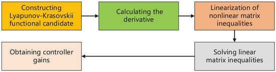
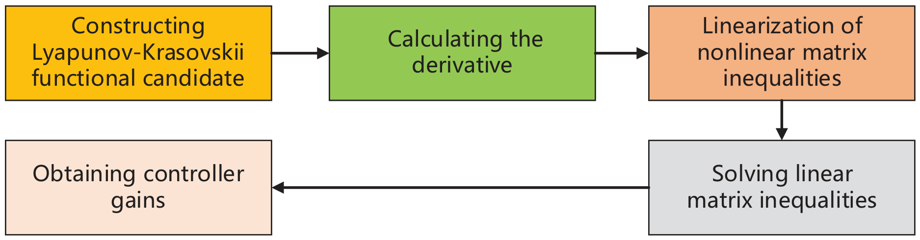
The constant-delay case $\phi \left(t\right)={\phi }_1$ is considered first. Conditions are derived for nonfragile stochastic tracking in the presence of the random nonlinear and uncertain terms. The main analytical steps appear in Figure 1.

Figure 1. Analysis procedure for the constant-delay case.

Theorem 1. 

Under Assumptions 1–4, take ${\epsilon }_1$, ${\epsilon }_2$, ϑ, q, ${\phi }_1$, and ${\varphi }_k(k=1,\dots ,4)$ as prescribed. Suppose that matrices $Q_1>0$, $R_1>0$, $R_2>0$, $M_1>0$, $M_2>0$, Q and scalars ${\delta }_1$, ${\delta }_2$, ${\sigma }_1$, ${\sigma }_2$ can be selected to fulfill

$$\begin{array}{c}\hfill \begin{array}{c}\mathrm{\Psi }=\left[\begin{array}{cccccccc}{\psi }_{11}& {\psi }_{12}& 0& {\psi }_{14}& {\psi }_{15}& {\psi }_{16}& {\psi }_{17}& I_Y\otimes Q_1\\ \ast & {\psi }_{22}& 0& 0& 0& {\psi }_{26}& {\psi }_{27}& 0\\ \ast & \ast & {\psi }_{33}& 0& 0& 0& 0& 0\\ \ast & \ast & \ast & -{\sigma }_1{\mathrm{\Sigma }}_1& 0& 0& 0& 0\\ \ast & \ast & \ast & \ast & -{\sigma }_2{\mathrm{\Sigma }}_2& 0& 0& 0\\ \ast & \ast & \ast & \ast & \ast & -{\sigma }_1{\mathrm{\Sigma }}_1& 0& 0\\ \ast & \ast & \ast & \ast & \ast & \ast & -{\sigma }_2{\mathrm{\Sigma }}_1& 0\\ \ast & \ast & \ast & \ast & \ast & \ast & \ast & -{\vartheta }^{-2}{\delta }_2{\mathrm{\Sigma }}_1\end{array}\right]<0,\hfill \\ Q_1<{\delta }_1{I}_p,\hfill \end{array}\end{array}$$

(13)

where

$$\begin{array}{c}\hfill \begin{array}{c}{\psi }_{11}=I_Y\otimes \left(\mathrm{Sym}(Q_1{\mathrm{\Gamma }}_1\right)+M_1+{\phi }_1^2{M}_2+{\delta }_1{\epsilon }_1^2{I}_p)-(1-q)\mathrm{Sym}(H\otimes B{R}_1),\hfill \\ {\psi }_{12}=I_Y\otimes Q_1{\mathrm{\Gamma }}_2-q(H\otimes B{R}_2),{\psi }_{22}=-I_Y\otimes M_1+{\delta }_2{\epsilon }_2^2{\mathrm{\Sigma }}_1,\hfill \\ {\psi }_{33}=-I_Y\otimes M_2,{\psi }_{14}=I_Y\otimes Q_1{E}_1,{\psi }_{15}=-H\otimes Q_{1}B{E}_2,{\mathrm{\Sigma }}_1=I_Y\otimes I_p,\hfill \\ {\psi }_{16}={\sigma }_1{\varphi }_1(I_Y\otimes F_1^T),{\psi }_{26}={\sigma }_1{\varphi }_2(I_Y\otimes F_2^T),{\mathrm{\Sigma }}_2=I_Y\otimes I_r,\hfill \\ {\psi }_{17}={\sigma }_2(1-q){\varphi }_3(I_Y\otimes F_3^T),{\psi }_{27}={\sigma }_{2}q{\varphi }_4(I_Y\otimes F_4^T),\hfill \end{array}\end{array}$$

then the constant-delay system (1) reaches nonfragile stochastic tracking under protocol (6), despite the stated random nonlinearities and uncertainties. Its gains are $K_1={\left(X^T\right)}^{-1}{\mathrm{\Phi }}^{-1}{Q}_{11}^{-1}\mathrm{\Phi }{X}^T{R}_1$ and $K_2={\left(X^T\right)}^{-1}{\mathrm{\Phi }}^{-1}{Q}_{11}^{-1}\mathrm{\Phi }{X}^T{R}_2$.

Proof. 

The proof starts from the following Lyapunov–Krasovskii functional candidate (LKFC) for (12):

$$\begin{array}{cc}\hfill \mathrm{\Xi }\left(t\right)=e^T\left(t\right)(I_Y\otimes Q_1)e\left(t\right)& +{\int }_{t-{\phi }_1}^t{e}^T\left(s\right)(I_Y\otimes M_1)e\left(s\right)ds\hfill \\ & +{\phi }_1{\int }_{-{\phi }_1}^0{\int }_{t+\theta }^t{e}^T\left(s\right)(I_Y\otimes M_2)e\left(s\right)dsd\theta .\hfill \end{array}$$

(14)

Introduce the infinitesimal operator $\mathcal{L}$ of $\mathrm{\Xi }\left(t\right)$ through

$$\begin{array}{c}\hfill \mathcal{L}\mathrm{\Xi }\left(t\right)=\underset{\nu \to 0^{+}}{\lim }{\displaystyle \frac{1}{\nu }}(\mathbf{E}\left\{\mathrm{\Xi }(t+\nu )\left|t\right.\right\}-\mathrm{\Xi }\left(t\right)),\end{array}$$

(15)

where an application of Ito’s formula to (14) produces

$$\begin{array}{c}\hfill d\mathrm{\Xi }\left(t\right)=\mathcal{L}\mathrm{\Xi }\left(t\right)dt+G\left(e\left(t\right)\right){\displaystyle \frac{\partial \mathrm{\Xi }\left(t\right)}{\partial e}}dw\left(t\right),\end{array}$$

(16)

the direct expansion of this generator results in

$$\begin{array}{cc}\hfill \mathcal{L}\mathrm{\Xi }\left(t\right)=& 2e^T\left(t\right)(I_Y\otimes Q_1)[I_Y\otimes ({\mathrm{\Gamma }}_1+({\varphi }_1\left(t\right)-{\varphi }_1)E_1{\overline{H}}_1\left(t\right)F_1+{\varphi }_1{E}_1{\overline{H}}_1\left(t\right)F_1)]e\left(t\right)\hfill \\ \hfill & -2e^T\left(t\right)(I_Y\otimes Q_1)[H\otimes (1-q)B(K_1+({\varphi }_3\left(t\right)-{\varphi }_3)E_2{\overline{H}}_2\left(t\right)F_3+{\varphi }_3{E}_2{\overline{H}}_2\left(t\right)F_3)]e\left(t\right)\hfill \\ \hfill & +2e^T\left(t\right)(I_Y\otimes Q_1)[I_Y\otimes ({\mathrm{\Gamma }}_2+({\varphi }_2\left(t\right)-{\varphi }_2)E_1{\overline{H}}_1\left(t\right)F_2+{\varphi }_2{E}_1{\overline{H}}_1\left(t\right)F_2)]e(t-{\phi }_1)\hfill \\ \hfill & -2e^T\left(t\right)(I_Y\otimes Q_1)[H\otimes qB(K_2+({\varphi }_4\left(t\right)-{\varphi }_4)E_2{\overline{H}}_2\left(t\right)F_4+{\varphi }_4\left(t\right)E_2{\overline{H}}_2\left(t\right)F_4)]e(t-{\phi }_1)\hfill \\ \hfill & +2e^T\left(t\right)(I_Y\otimes Q_1)[(\vartheta \left(t\right)-\vartheta )F\left(e(t-{\phi }_1)\right)+\vartheta F\left(e(t-{\phi }_1)\right)]\hfill \\ \hfill & +e^T\left(t\right)(I_Y\otimes M_1)e\left(t\right)-e^T(t-{\phi }_1)(I_Y\otimes M_1)e(t-{\phi }_1)\hfill \\ \hfill & +{\phi }_1^2{e}^T\left(t\right)(I_Y\otimes M_2)e\left(t\right)-{\phi }_1{\int }_{t-{\phi }_1}^t{e}^T\left(s\right)(I_Y\otimes M_2)e\left(s\right)ds\hfill \\ \hfill & +\mathrm{Tr}\left[G^T\left(e\left(t\right)\right)(I_Y\otimes Q_1)G\left(e\left(t\right)\right)\right],\hfill \end{array}$$

(17)

and from Assumption 4, $G^T\left(e\left(t\right)\right)G\left(e\left(t\right)\right)\le {\epsilon }_1^2{e}^T\left(t\right)e\left(t\right)$ and $F^T\left(e\left(t\right)\right)F\left(e\left(t\right)\right)\le {\epsilon }_2^2{e}^T\left(t\right)e\left(t\right)$. Using these bounds with (13) and (17) gives

$$\begin{array}{c}\hfill \mathrm{Tr}\left[G^T\left(e\left(t\right)\right)(I_Y\otimes Q_1)G\left(e\left(t\right)\right)\right]\le {\lambda }_{\max }\left(Q_1\right)\mathrm{Tr}\left[G^T\left(e\left(t\right)\right)G\left(e\left(t\right)\right)\right]\le {\delta }_1{\epsilon }_1^2{e}^T\left(t\right)e\left(t\right),\end{array}$$

(18)

the nonlinear cross term in (17) admits the additional estimate

$$\begin{array}{c}\hfill 2\vartheta e^T\left(t\right)(I_Y\otimes Q_1)F\left(e(t-{\phi }_1)\right)\le {\delta }_2^{-1}{\vartheta }^2{e}^T\left(t\right)(I_Y\otimes Q_1^T{Q}_1)e\left(t\right)+{\delta }_2{\epsilon }_2^2{e}^T(t-{\phi }_1)e(t-{\phi }_1),\end{array}$$

(19)

and for the integral term, Lemma 3 gives

$$\begin{array}{c}\hfill -{\phi }_1{\int }_{t-{\phi }_1}^t{e}^T\left(s\right)(I_Y\otimes M_2)e\left(s\right)ds\le -\left({\int }_{t-{\phi }_1}^{t}e\left(s\right)ds{)}^T(I_Y\otimes M_2)({\int }_{t-{\phi }_1}^{t}e\left(s\right)ds\right).\end{array}$$

(20)

From (5) and (10), we can deduce the following: $\mathbf{E}\left\{\vartheta \right(t)-\vartheta \}=0$, $\mathbf{E}\{{\varphi }_k\left(t\right)-{\varphi }_k\}=0,(k=1,\dots ,4).$ Define $\xi \left(t\right)=\mathrm{col}(e\left(t\right),e(t-{\phi }_1),{\int }_{t-{\phi }_1}^{t}e\left(s\right)ds)$. After (17)–(20) are combined, the estimate becomes

$$\begin{array}{c}\hfill \mathbf{E}\left\{\mathcal{L}\mathrm{\Xi }\left(t\right)\right\}\le \mathbf{E}\left\{{\xi }^T\left(t\right)(\mathrm{\Pi }+\Delta \mathrm{\Pi })\xi \left(t\right)\right\},\end{array}$$

(21)

where

$$\begin{array}{c}\hfill \begin{array}{c}\mathrm{\Pi }=\left[\begin{array}{ccc}{\pi }_{11}& {\pi }_{12}& 0\\ \ast & {\pi }_{22}& 0\\ \ast & \ast & -I_Y\otimes M_2\end{array}\right],\hfill \\ \Delta \mathrm{\Pi }=\mathrm{Sym}({\overline{\mathrm{\Omega }}}_1{\overline{H}}_1\left(t\right){\tilde{\mathrm{\Omega }}}_1+{\overline{\mathrm{\Omega }}}_2{\overline{H}}_2\left(t\right){\tilde{\mathrm{\Omega }}}_2),\hfill \end{array}\end{array}$$

with

$$\begin{array}{c}\hfill \begin{array}{c}{\pi }_{11}=I_Y\otimes \left(\mathrm{Sym}(Q_1{\mathrm{\Gamma }}_1\right)+M_1+{\phi }_1^2{M}_2+{\delta }_1{\epsilon }_1^2{I}_p+{\delta }_2^{-1}{\vartheta }^2{Q}_1^T{Q}_1)-(1-q)\mathrm{Sym}(H\otimes Q_{1}B{K}_1),\hfill \\ {\pi }_{12}=I_Y\otimes Q_1{\mathrm{\Gamma }}_2-q(H\otimes Q_{1}B{K}_2),{\pi }_{22}=-I_Y\otimes M_1+{\delta }_2{\epsilon }_2^2{\mathrm{\Sigma }}_1,\hfill \\ {\overline{\mathrm{\Omega }}}_1=\mathrm{col}(I_Y\otimes Q_1{E}_1,0,0),{\overline{\mathrm{\Omega }}}_2=\mathrm{col}(-H\otimes Q_{1}B{E}_2,0,0),\hfill \\ {\tilde{\mathrm{\Omega }}}_1=[{\varphi }_1{I}_Y\otimes F_1,{\varphi }_2{I}_Y\otimes F_2,0],{\tilde{\mathrm{\Omega }}}_2=[(1-q){\varphi }_3{I}_Y\otimes F_3,q{\varphi }_4{I}_Y\otimes F_4,0].\hfill \end{array}\end{array}$$

Lemma 2 removes the norm-bounded uncertainty from the estimate based on (17), yielding

$$\begin{array}{c}\hfill \mathbf{E}\left\{\mathcal{L}\mathrm{\Xi }\left(t\right)\right\}\le \mathbf{E}\left\{{\xi }^T\left(t\right)(\mathrm{\Pi }+{\sigma }_1{\tilde{\mathrm{\Omega }}}_1^T{\tilde{\mathrm{\Omega }}}_1+{\sigma }_1^{-1}{\overline{\mathrm{\Omega }}}_1{\overline{\mathrm{\Omega }}}_1^T+{\sigma }_2{\tilde{\mathrm{\Omega }}}_2^T{\tilde{\mathrm{\Omega }}}_2+{\sigma }_2^{-1}{\overline{\mathrm{\Omega }}}_2{\overline{\mathrm{\Omega }}}_2^T)\xi \left(t\right)\right\}.\end{array}$$

(22)

The identity $BQ=Q_{1}B$ follows from Lemma 1. It determines Q through

$$\begin{array}{c}\hfill Q_1{V}^T\left[\begin{array}{c}\mathrm{\Phi }\\ 0\end{array}\right]X^T=V^T\left[\begin{array}{c}\mathrm{\Phi }\\ 0\end{array}\right]X^{T}Q,\end{array}$$

an equivalent expression is

$$\begin{array}{c}\hfill V^T\left[\begin{array}{cc}{Q}_{11}& 0\\ 0& Q_{22}\end{array}\right]\left[\begin{array}{c}\mathrm{\Phi }\\ 0\end{array}\right]X^T=V^T\left[\begin{array}{c}\mathrm{\Phi }\\ 0\end{array}\right]X^{T}Q,\end{array}$$

from which

$$\begin{array}{c}\hfill Q={\left(X^T\right)}^{-1}{\mathrm{\Phi }}^{-1}{Q}_{11}\mathrm{\Phi }{X}^T,\end{array}$$

and the relations used in Theorem 1 are $BQ=Q_{1}B$, $R_1=Q{K}_1$ and $R_2=Q{K}_2$. The Schur complement of $\mathrm{\Psi }<0$ in (13) is

$$\begin{array}{c}\hfill \mathrm{\Pi }+{\sigma }_1{\tilde{\mathrm{\Omega }}}_1^T{\tilde{\mathrm{\Omega }}}_1+{\sigma }_1^{-1}{\overline{\mathrm{\Omega }}}_1{\overline{\mathrm{\Omega }}}_1^T+{\sigma }_2{\tilde{\mathrm{\Omega }}}_2^T{\tilde{\mathrm{\Omega }}}_2+{\sigma }_2^{-1}{\overline{\mathrm{\Omega }}}_2{\overline{\mathrm{\Omega }}}_2^T<0.\end{array}$$

(23)

After expectation is applied to (16), one obtains

$$\begin{array}{c}\hfill \mathbf{E}\left\{\mathcal{L}\mathrm{\Xi }\left(t\right)\right\}\le \mathbf{E}\left\{{\xi }^T\left(t\right)\mathrm{\Psi }\xi \left(t\right)\right\},\end{array}$$

(24)

and condition (13) makes $\mathbf{E}\left\{\mathcal{L}\mathrm{\Xi }\right(t\left)\right\}<0$. Thus, a constant μ can be chosen so that

$$\begin{array}{c}\hfill \mathbf{E}\left\{\mathcal{L}\mathrm{\Xi }\left(t\right)\right\}\le -\mu \mathbf{E}\left\{{∥e\left(t\right)∥}^2\right\}.\end{array}$$

(25)

By Lemma 1 in [43], the error dynamics (11) are asymptotically stable in mean square [26,35,44]. This establishes the claimed nonfragile stochastic tracking for the delayed nonlinear MASs. Dimensions of the blocks in (13) are listed in Table 1, which concludes the proof of Theorem 1. □

Table 1. Block dimensions in (13).

${\psi }_{11}$	${\psi }_{12}$	${\psi }_{14}$	${\psi }_{15}$	${\psi }_{16}$	${\psi }_{17}$
$Yp\times Yp$	$Yp\times Yp$	$Yp\times Yp$	$Yp\times Yr$	$Yp\times Yp$	$Yp\times Yp$
${\psi }_{22}$	${\psi }_{26}$	${\psi }_{27}$	${\psi }_{33}$	${\mathrm{\Sigma }}_1$	${\mathrm{\Sigma }}_2$
$Yp\times Yp$	$Yp\times Yp$	$Yp\times Yp$	$Yp\times Yp$	$Yp\times Yp$	$Yr\times Yr$

Remark 3. 

When ${\phi }_1=0$, model (1) has the delay-free form

$$\begin{array}{c}\hfill \begin{array}{c}d{x}_0\left(t\right)=[{\mathrm{\Gamma }}_1\left(t\right)x_0\left(t\right)+\vartheta \left(t\right)f\left(x_0\left(t\right)\right)]dt+g\left(x_0\left(t\right)\right)d\omega \left(t\right),\hfill \\ d{x}_i\left(t\right)=[{\mathrm{\Gamma }}_1\left(t\right)x_i\left(t\right)+\vartheta \left(t\right)f\left(x_i\left(t\right)\right)+B{u}_i\left(t\right)]dt+g\left(x_i\left(t\right)\right)d\omega \left(t\right),\hfill \end{array}\end{array}$$

and with the delay removed, (6) reduces to $u_i\left(t\right)=-(1-q)K_1\left(t\right)m_i\left(t\right)$. The corresponding conclusion follows by taking $\mathrm{\Xi }\left(t\right)=e^T\left(t\right)(I_Y\otimes Q_1)e\left(t\right)$ as the LKFC.

Corollary 1. 

Assume that Assumptions 1–4 are valid and that ${\epsilon }_1$, ϑ, q, ${\varphi }_1$, and ${\varphi }_3$ are prescribed. If matrices $Q_1>0$, $R_1>0$ and scalars ${\delta }_1$, ${\delta }_2$, ${\sigma }_1$, ${\sigma }_2$ can be chosen to satisfy

$$\begin{array}{c}\hfill \begin{array}{c}\tilde{\mathrm{\Psi }}=\left[\begin{array}{cccccc}{\tilde{\psi }}_{11}& {\tilde{\psi }}_{12}& {\tilde{\psi }}_{13}& {\tilde{\psi }}_{14}& {\tilde{\psi }}_{15}& I_Y\otimes Q_1\\ \ast & -{\sigma }_1{\mathrm{\Sigma }}_1& 0& 0& 0& 0\\ \ast & \ast & -{\sigma }_2{\mathrm{\Sigma }}_2& 0& 0& 0\\ \ast & \ast & \ast & -{\sigma }_1{\mathrm{\Sigma }}_1& 0& 0\\ \ast & \ast & \ast & \ast & -{\sigma }_2{\mathrm{\Sigma }}_1& 0\\ \ast & \ast & \ast & \ast & \ast & -{\vartheta }^{-2}{\delta }_2{\mathrm{\Sigma }}_1\end{array}\right]<0,\hfill \\ Q_1<{\delta }_1{I}_p,\hfill \end{array}\end{array}$$

where

$$\begin{array}{c}\hfill \begin{array}{c}{\tilde{\psi }}_{11}=I_Y\otimes (\mathrm{Sym}\left(Q_1{\mathrm{\Gamma }}_1\right)+{\delta }_1{\epsilon }_1^2{I}_p)-(1-q)\mathrm{Sym}(H\otimes B{R}_1),\hfill \\ {\tilde{\psi }}_{12}=I_Y\otimes Q_1{E}_1,{\tilde{\psi }}_{13}=-H\otimes Q_{1}B{E}_2,{\tilde{\psi }}_{14}={\sigma }_1{\varphi }_1(I_Y\otimes F_1^T),\hfill \\ {\mathrm{\Sigma }}_1=I_Y\otimes I_p,{\mathrm{\Sigma }}_2=I_Y\otimes I_r,{\tilde{\psi }}_{15}={\sigma }_2(1-q){\varphi }_3(I_Y\otimes F_3^T),\hfill \end{array}\end{array}$$

then the delay-free version of (1) achieves nonfragile stochastic tracking under (6). Its controller gain is $K_1={\left(X^T\right)}^{-1}{\mathrm{\Phi }}^{-1}{Q}_{11}^{-1}\mathrm{\Phi }{X}^T{R}_1$.

3.2. Conditions for Nonfragile Stochastic Tracking Under TVDs

We next allow the delay to vary with time, without removing the randomly activated nonlinear and uncertain terms.

Theorem 2. 

Let Assumptions 1–4 be in force, with ${\tilde{\epsilon }}_1$, ${\tilde{\epsilon }}_2$, ϑ, q, $\widehat{\phi }$ and ${\varphi }_k(k=1,\dots ,4)$ prescribed. Assume that matrices ${\tilde{Q}}_1>0$, ${\tilde{R}}_1>0$, ${\tilde{R}}_2>0$, ${\tilde{M}}_1>0$, Q and scalars ${\tilde{\delta }}_1$, ${\tilde{\delta }}_2$, ${\tilde{\sigma }}_1$, ${\tilde{\sigma }}_2$ satisfy

$$\begin{array}{c}\hfill \begin{array}{c}\mathrm{\Theta }=\left[\begin{array}{ccccccc}{\theta }_{11}& {\theta }_{12}& {\theta }_{13}& {\theta }_{14}& {\theta }_{15}& {\theta }_{16}& I_Y\otimes {\tilde{Q}}_1\\ \ast & {\theta }_{22}& 0& 0& {\theta }_{25}& {\theta }_{26}& 0\\ \ast & \ast & -{\tilde{\sigma }}_1{\mathrm{\Sigma }}_1& 0& 0& 0& 0\\ \ast & \ast & \ast & -{\tilde{\sigma }}_2{\mathrm{\Sigma }}_2& 0& 0& 0\\ \ast & \ast & \ast & \ast & -{\tilde{\sigma }}_1{\mathrm{\Sigma }}_1& 0& 0\\ \ast & \ast & \ast & \ast & \ast & -{\tilde{\sigma }}_2{\mathrm{\Sigma }}_1& 0\\ \ast & \ast & \ast & \ast & \ast & \ast & -{\vartheta }^{-2}{\tilde{\delta }}_2{\mathrm{\Sigma }}_1\end{array}\right]<0,\hfill \\ {\tilde{Q}}_1<{\tilde{\delta }}_1{I}_p,\hfill \end{array}\end{array}$$

(26)

where

$$\begin{array}{c}\hfill \begin{array}{c}{\theta }_{11}=I_Y\otimes \left(\mathrm{Sym}({\tilde{Q}}_1{\mathrm{\Gamma }}_1\right)+{\tilde{M}}_1+{\tilde{\delta }}_1{\tilde{\epsilon }}_1^2{I}_p)-(1-q)\mathrm{Sym}(H\otimes B{\tilde{R}}_1),\hfill \\ {\theta }_{12}=I_Y\otimes {\tilde{Q}}_1{\mathrm{\Gamma }}_2-q(H\otimes B{\tilde{R}}_2),{\theta }_{22}=-(1-\widehat{\phi })(I_Y\otimes {\tilde{M}}_1)+{\tilde{\delta }}_2{\tilde{\epsilon }}_2^2{\mathrm{\Sigma }}_1,\hfill \\ {\theta }_{13}=I_Y\otimes {\tilde{Q}}_1{E}_1,{\theta }_{14}=-H\otimes {\tilde{Q}}_{1}B{E}_2,{\mathrm{\Sigma }}_1=I_Y\otimes I_p,\hfill \\ {\theta }_{15}={\tilde{\sigma }}_1{\varphi }_1(I_Y\otimes F_1^T),{\theta }_{25}={\tilde{\sigma }}_1{\varphi }_2(I_Y\otimes F_2^T),{\mathrm{\Sigma }}_2=I_Y\otimes I_r,\hfill \\ {\theta }_{16}={\tilde{\sigma }}_2(1-q){\varphi }_3(I_Y\otimes F_3^T),{\theta }_{26}={\tilde{\sigma }}_{2}q{\varphi }_4(I_Y\otimes F_4^T),\hfill \end{array}\end{array}$$

then the delayed nonlinear MASs (1) achieve nonfragile stochastic tracking under protocol (6), with TVDs and the randomly occurring nonlinearities and uncertainties. The controller matrices are recovered from $K_1=Q^{-1}{\tilde{R}}_1$, $K_2=Q^{-1}{\tilde{R}}_2$, and $BQ={\tilde{Q}}_{1}B$.

Proof. 

For (12), choose the LKFC

$$\begin{array}{c}\hfill \tilde{\mathrm{\Xi }}\left(t\right)=e^T\left(t\right)(I_Y\otimes {\tilde{Q}}_1)e\left(t\right)+{\int }_{t-\phi \left(t\right)}^t{e}^T\left(s\right)(I_Y\otimes {\tilde{M}}_1)e\left(s\right)ds.\end{array}$$

(27)

Evaluating (27) by Ito’s formula gives

$$\begin{array}{c}\hfill d\tilde{\mathrm{\Xi }}\left(t\right)=\mathcal{L}\tilde{\mathrm{\Xi }}\left(t\right)dt+G\left(e\left(t\right)\right){\displaystyle \frac{\partial \tilde{\mathrm{\Xi }}\left(t\right)}{\partial e}}dw\left(t\right),\end{array}$$

(28)

and the resulting infinitesimal generator can be written as

$$\begin{array}{cc}\hfill \mathcal{L}\tilde{\mathrm{\Xi }}\left(t\right)=& 2e^T\left(t\right)(I_Y\otimes {\tilde{Q}}_1)[I_Y\otimes ({\mathrm{\Gamma }}_1+({\varphi }_1\left(t\right)-{\varphi }_1)E_1{\overline{H}}_1\left(t\right)F_1+{\varphi }_1{E}_1{\overline{H}}_1\left(t\right)F_1)]e\left(t\right)\hfill \\ \hfill & -2e^T\left(t\right)(I_Y\otimes {\tilde{Q}}_1)[H\otimes (1-q)B(K_1+({\varphi }_3\left(t\right)-{\varphi }_3)E_2{\overline{H}}_2\left(t\right)F_3+{\varphi }_3{E}_2{\overline{H}}_2\left(t\right)F_3)]e\left(t\right)\hfill \\ \hfill & +2e^T\left(t\right)(I_Y\otimes {\tilde{Q}}_1)[I_Y\otimes ({\mathrm{\Gamma }}_2+({\varphi }_2\left(t\right)-{\varphi }_2)E_1{\overline{H}}_1\left(t\right)F_2+{\varphi }_2{E}_1{\overline{H}}_1\left(t\right)F_2)]e(t-\phi \left(t\right))\hfill \\ \hfill & -2e^T\left(t\right)(I_Y\otimes {\tilde{Q}}_1)[H\otimes qB(K_2+({\varphi }_4\left(t\right)-{\varphi }_4)E_2{\overline{H}}_2\left(t\right)F_4+{\varphi }_4{E}_2{\overline{H}}_2\left(t\right)F_4)]e(t-\phi \left(t\right))\hfill \\ \hfill & +2e^T\left(t\right)(I_Y\otimes {\tilde{Q}}_1)[(\vartheta \left(t\right)-\vartheta )F\left(e(t-\phi \left(t\right))\right)+\vartheta F\left(e(t-\phi \left(t\right))\right)]\hfill \\ \hfill & +e^T\left(t\right)(I_Y\otimes {\tilde{M}}_1)e\left(t\right)-(1-\dot{\phi }\left(t\right))e^T(t-\phi \left(t\right))(I_Y\otimes {\tilde{M}}_1)e(t-\phi \left(t\right))\hfill \\ \hfill & +\mathrm{Tr}\left[G^T\left(e\left(t\right)\right)(I_Y\otimes {\tilde{Q}}_1)G\left(e\left(t\right)\right)\right].\hfill \end{array}$$

(29)

Assumption 4 supplies $G^T\left(e\left(t\right)\right)G\left(e\left(t\right)\right)\le {\tilde{\epsilon }}_1^2{e}^T\left(t\right)e\left(t\right)$ and $F^T\left(e\left(t\right)\right)F\left(e\left(t\right)\right)\le {\tilde{\epsilon }}_2^2{e}^T\left(t\right)e\left(t\right)$. In conjunction with (26) and (29), these inequalities imply

$$\begin{array}{c}\hfill \mathrm{Tr}\left[G^T\left(e\left(t\right)\right)(I_Y\otimes {\tilde{Q}}_1)G\left(e\left(t\right)\right)\right]\le {\lambda }_{\max }\left({\tilde{Q}}_1\right)\mathrm{Tr}\left[G^T\left(e\left(t\right)\right)G\left(e\left(t\right)\right)\right]\le {\tilde{\delta }}_1{\tilde{\epsilon }}_1^2{e}^T\left(t\right)e\left(t\right),\end{array}$$

(30)

and a further consequence of (29) is

$$\begin{array}{c}\hfill 2\vartheta e^T\left(t\right)(I_Y\otimes {\tilde{Q}}_1)F\left(e(t-\phi \left(t\right))\right)\le {\tilde{\delta }}_2^{-1}{\vartheta }^2{e}^T\left(t\right)(I_Y\otimes {\tilde{Q}}_1^T{\tilde{Q}}_1)e\left(t\right)+{\tilde{\delta }}_2{\tilde{\epsilon }}_2^2{e}^T(t-\phi \left(t\right))e(t-\phi \left(t\right)).\end{array}$$

(31)

Introduce $\zeta \left(t\right)=\mathrm{col}\left(e\right(t),e(t-\phi \left(t\right)\left)\right)$. Applying the same bounding argument as in Theorem 1 to (29)–(31) yields

$$\begin{array}{c}\hfill \mathbf{E}\left\{\mathcal{L}\tilde{\mathrm{\Xi }}\left(t\right)\right\}\le \mathbf{E}\left\{{\zeta }^T\left(t\right)(\tilde{\mathrm{\Pi }}+\Delta \tilde{\mathrm{\Pi }})\zeta \left(t\right)\right\},\end{array}$$

(32)

where

$$\begin{array}{c}\hfill \begin{array}{c}\tilde{\mathrm{\Pi }}=\left[\begin{array}{cc}{\tilde{\pi }}_{11}& {\tilde{\pi }}_{12}\\ \ast & {\tilde{\pi }}_{22}\end{array}\right],\hfill \\ \Delta \tilde{\mathrm{\Pi }}=\mathrm{Sym}({\overline{\mathrm{\Lambda }}}_1{\overline{H}}_1\left(t\right){\tilde{\mathrm{\Lambda }}}_1+{\overline{\mathrm{\Lambda }}}_2{\overline{H}}_2\left(t\right){\tilde{\mathrm{\Lambda }}}_2),\hfill \end{array}\end{array}$$

with

$$\begin{array}{c}\hfill \begin{array}{c}{\tilde{\pi }}_{11}=I_Y\otimes \left(\mathrm{Sym}({\tilde{Q}}_1{\mathrm{\Gamma }}_1\right)+{\tilde{M}}_1+{\tilde{\delta }}_1{\tilde{\epsilon }}_1^2{I}_p+{\tilde{\delta }}_2^{-1}{\vartheta }^2{\tilde{Q}}_1^T{\tilde{Q}}_1)-(1-q)\mathrm{Sym}(H\otimes {\tilde{Q}}_{1}B{K}_1),\hfill \\ {\tilde{\pi }}_{12}=I_Y\otimes {\tilde{Q}}_1{\mathrm{\Gamma }}_2-q(H\otimes {\tilde{Q}}_{1}B{K}_2),{\tilde{\pi }}_{22}=-(1-\widehat{\phi })(I_Y\otimes {\tilde{M}}_1)+{\tilde{\delta }}_2{\tilde{\epsilon }}_2^2{\mathrm{\Sigma }}_1,\hfill \\ {\overline{\mathrm{\Lambda }}}_1=\mathrm{col}(I_Y\otimes {\tilde{Q}}_1{E}_1,0),{\tilde{\mathrm{\Lambda }}}_1=[{\varphi }_1{I}_Y\otimes F_1,{\varphi }_2{I}_Y\otimes F_2],\hfill \\ {\overline{\mathrm{\Lambda }}}_2=\mathrm{col}(-H\otimes {\tilde{Q}}_{1}B{E}_2,0),{\tilde{\mathrm{\Lambda }}}_2=[(1-q){\varphi }_3{I}_Y\otimes F_3,q{\varphi }_4{I}_Y\otimes F_4].\hfill \end{array}\end{array}$$

Using Lemma 2, inequality (32) becomes

$$\begin{array}{c}\hfill \mathbf{E}\left\{\mathcal{L}\tilde{\mathrm{\Xi }}\left(t\right)\right\}\le \mathbf{E}\left\{{\zeta }^T\left(t\right)(\tilde{\mathrm{\Pi }}+{\tilde{\sigma }}_1{\tilde{\mathrm{\Lambda }}}_1^T{\tilde{\mathrm{\Lambda }}}_1+{\tilde{\sigma }}_1^{-1}{\overline{\mathrm{\Lambda }}}_1{\overline{\mathrm{\Lambda }}}_1^T+{\tilde{\sigma }}_2{\tilde{\mathrm{\Lambda }}}_2^T{\tilde{\mathrm{\Lambda }}}_2+{\tilde{\sigma }}_2^{-1}{\overline{\mathrm{\Lambda }}}_2{\overline{\mathrm{\Lambda }}}_2^T)\zeta \left(t\right)\right\},\end{array}$$

(33)

and as in Theorem 1, the construction provides $BQ={\tilde{Q}}_{1}B$, ${\tilde{R}}_1=Q{K}_1$ and ${\tilde{R}}_2=Q{K}_2$. Taking the Schur complement of $\mathrm{\Theta }<0$ in (26) gives

$$\begin{array}{c}\hfill \tilde{\mathrm{\Pi }}+{\tilde{\sigma }}_1{\tilde{\mathrm{\Lambda }}}_1^T{\tilde{\mathrm{\Lambda }}}_1+{\tilde{\sigma }}_1^{-1}{\overline{\mathrm{\Lambda }}}_1{\overline{\mathrm{\Lambda }}}_1^T+{\tilde{\sigma }}_2{\tilde{\mathrm{\Lambda }}}_2^T{\tilde{\mathrm{\Lambda }}}_2+{\tilde{\sigma }}_2^{-1}{\overline{\mathrm{\Lambda }}}_2{\overline{\mathrm{\Lambda }}}_2^T<0.\end{array}$$

(34)

The same expectation argument used for Theorem 1 gives $\mathbf{E}\left\{\mathcal{L}\tilde{\mathrm{\Xi }}\left(t\right)\right\}\le \mathbf{E}\left\{{\varsigma }^T\left(t\right)\mathrm{\Theta }\varsigma \left(t\right)\right\}$. Because of (26), $\mathbf{E}\left\{\mathcal{L}\tilde{\mathrm{\Xi }}\left(t\right)\right\}<0$; moreover, there is a $\tilde{\mu }$ satisfying $\mathbf{E}\left\{\mathcal{L}\tilde{\mathrm{\Xi }}\left(t\right)\right\}\le -\tilde{\mu }\mathbf{E}\left\{{∥e\left(t\right)∥}^2\right\}$. It follows that (11) is mean-square asymptotically stable [26,35,44]. Nonfragile stochastic tracking under TVDs is therefore established. Table 2 gives the dimensions of the blocks in (26), completing the proof of Theorem 2. □

Table 2. Block dimensions in (26).

${\theta }_{11}$	${\theta }_{12}$	${\theta }_{13}$	${\theta }_{14}$	${\theta }_{15}$	${\theta }_{16}$
$Yp\times Yp$	$Yp\times Yp$	$Yp\times Yp$	$Yp\times Yr$	$Yp\times Yp$	$Yp\times Yp$
${\theta }_{22}$	${\theta }_{25}$	${\theta }_{26}$	${\mathrm{\Sigma }}_1$	${\mathrm{\Sigma }}_2$	$I_Y\otimes {\tilde{Q}}_1$
$Yp\times Yp$	$Yp\times Yp$	$Yp\times Yp$	$Yp\times Yp$	$Yr\times Yr$	$Yp\times Yp$

Remark 4. 

The unknown matrices and the gains in Theorems 1 and 2 are obtained by solving (13) and (26). These linear matrix inequalities (LMIs) avoid the need for an eigenvalue of the structure matrix H, unlike the construction in [26]. As Y grows, however, both LMIs (13) and (26) increase in dimension. A lower-cost formulation is therefore left for future study.

4. Simulation Results

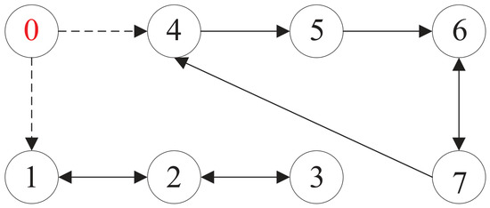
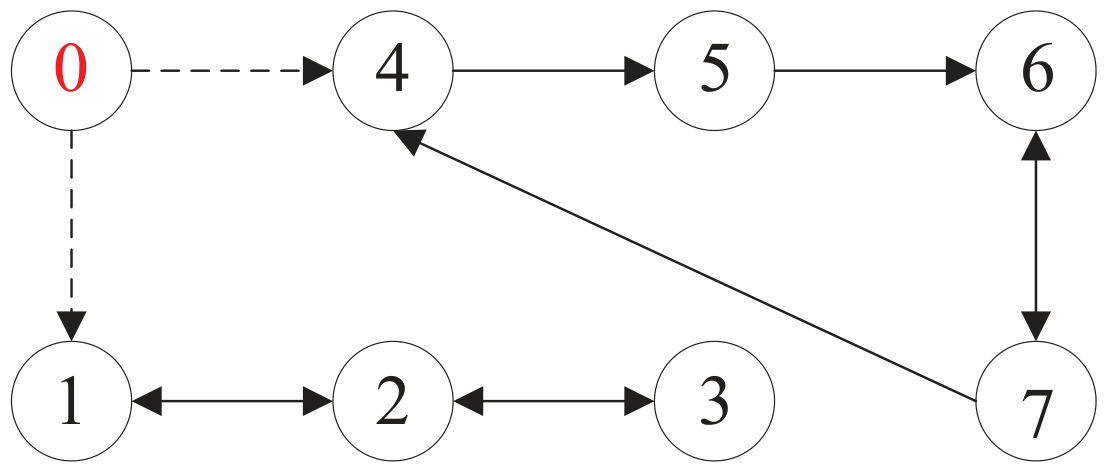
The two theorems are examined through separate numerical cases. In the network of Figure 2, node 0 reaches all other nodes through a directed tree, and nodes 1–7 are the followers.

Figure 2. Directed interaction network adopted in the simulations.

Example 1. 

To examine Theorem 1, take $x_{i1}$, $x_{i2}$, and $x_{i3}$ from $[-2020]\times [-2020]\times [-2020]$. The matrices used in this case are

$$\begin{array}{c}\hfill \begin{array}{c}{\mathrm{\Gamma }}_1=\left[\begin{array}{ccc}-3.5& -1.6& -1.5\\ 4.9& -1.7& 0.8\\ -0.7& -1.3& -3.7\end{array}\right],{\mathrm{\Gamma }}_2=\left[\begin{array}{ccc}2& 1& -1\\ 0.5& 0.5& 0.2\\ 0.3& 0.3& -0.5\end{array}\right],B=\left[\begin{array}{c}1\\ 2\\ 0\end{array}\right],\hfill \\ F_1=\mathrm{diag}\{0.01,0.01,0.02\},F_2=\mathrm{diag}\{0.01,-0.01,0.03\},E_1=\mathrm{diag}\{0.01,-0.01,-0.01\},\hfill \\ F_3=\mathrm{diag}\{0.02,-0.03,0.02\},F_4=\mathrm{diag}\{0.02,-0.02,0.02\},E_2=0.01.\hfill \end{array}\end{array}$$

Use $q=0.5$, $\vartheta =0.3$, ${\epsilon }_1=0.5$, ${\epsilon }_2=0.7$, ${\varphi }_1=0.5$, ${\varphi }_2=0.3$, ${\varphi }_3=0.4$, ${\varphi }_4=0.5$, and ${\phi }_1=0.37$ for the remaining quantities.

The feasibility of (13) is checked with feasp in MATLAB R2024a, giving

$$\begin{array}{c}\hfill \begin{array}{c}{\sigma }_1=9.5773,{\sigma }_2=9.5771,{\delta }_1=6.1895,{\delta }_2=0.9234,Q=1.2254,\hfill \\ Q_1=\left[\begin{array}{ccc}2.1857& -0.4802& -0.7041\\ -0.4802& 1.4655& 0.3520\\ -0.7041& 0.3520& 3.1629\end{array}\right],R_1={\left[\begin{array}{c}3.3563\\ 7.2019\\ -0.8140\end{array}\right]}^T,R_2={\left[\begin{array}{c}0.7424\\ 0.5071\\ -0.1002\end{array}\right]}^T,\hfill \\ M_1=\left[\begin{array}{ccc}8.1479& -1.0285& -0.8160\\ -1.0285& 4.8643& 0.9830\\ -0.8160& 0.9830& 8.8122\end{array}\right],M_2=\left[\begin{array}{ccc}8.7984& -0.6576& 0.0470\\ -0.6576& 7.9108& 0.4116\\ 0.0470& 0.4116& 9.2657\end{array}\right],\hfill \end{array}\end{array}$$

and the gains recovered from Theorem 1 are $K_1$ and $K_2$ as shown below:

$$\begin{array}{c}\hfill K_1=\left[\begin{array}{ccc}2.7389& 5.8770& -0.6642\end{array}\right],K_2=\left[\begin{array}{ccc}0.6058& 0.4138& -0.0817\end{array}\right].\end{array}$$

For the computed matrices, report the residual ${∥BQ-Q_{1}B∥}_2$ together with the largest eigenvalue of $\mathrm{\Psi }$:

$$\begin{array}{c}\hfill {∥BQ-Q_{1}B∥}_2=1.666\times {10}^{-4},{\lambda }_{\max }\left(\mathrm{\Psi }\right)=-0.1865.\end{array}$$

For this example, specify $f\left(x_i(t-{\phi }_1)\right)$ and $g\left(x_i\left(t\right)\right)$ by

$$\begin{array}{c}\hfill \begin{array}{c}f\left(x_i(t-{\phi }_1)\right)={[0.5\sin \left(x_{i1}(t-{\phi }_1)\right),0.5\sin \left(x_{i2}(t-{\phi }_1)\right),0.5\sin \left(x_{i3}(t-{\phi }_1)\right)]}^T,\hfill \\ g\left(x_i\left(t\right)\right)={[0.2\sin \left(x_{i1}\left(t\right)\right),0.2\sin \left(x_{i2}\left(t\right)\right),0.2\sin \left(x_{i3}\left(t\right)\right)]}^T.\hfill \end{array}\end{array}$$

The convergence rate, maximum tracking deviation, and integrated mean-square error (IMSE) are reported for both controllers in Table 3.

Table 3. Quantitative comparison of the two controllers.

Controller Case	Convergence Rate	Peak Tracking Error	IMSE
Nonfragile	0.9202	11.3578	83.1969
Conventional	0.8149	11.3578	94.4274

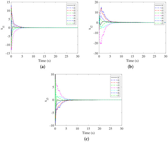
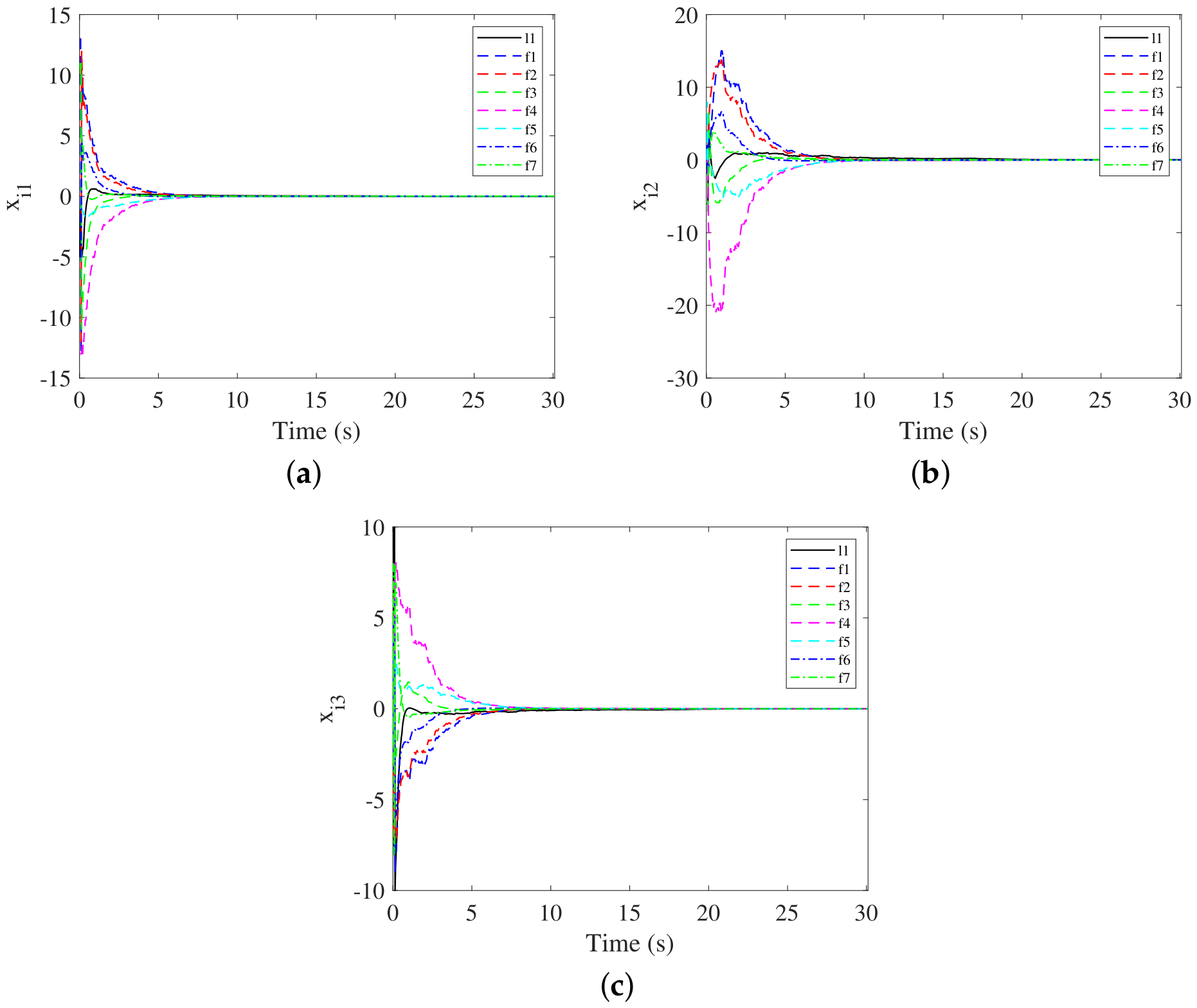
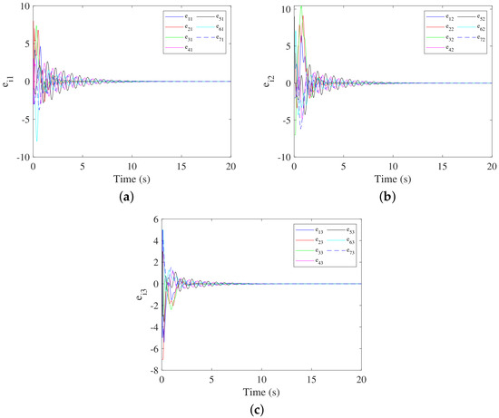
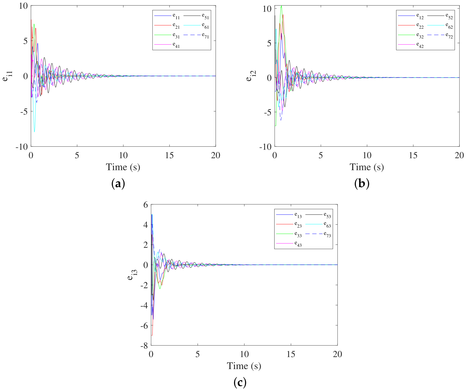
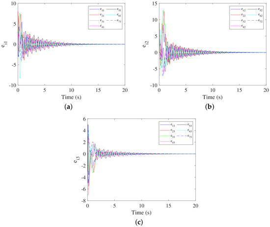
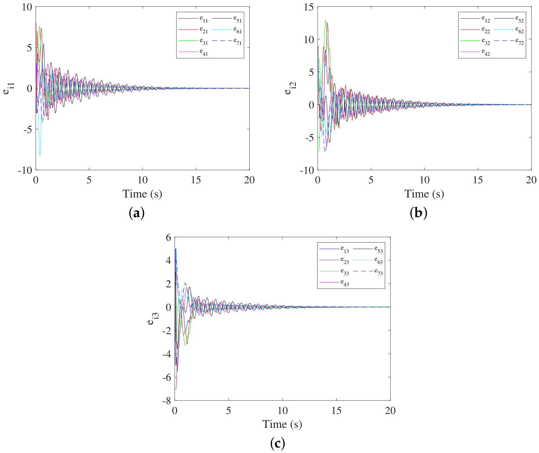
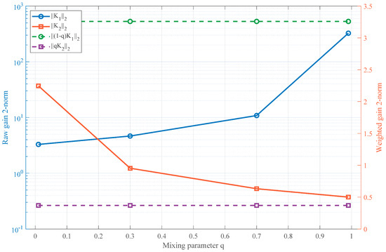
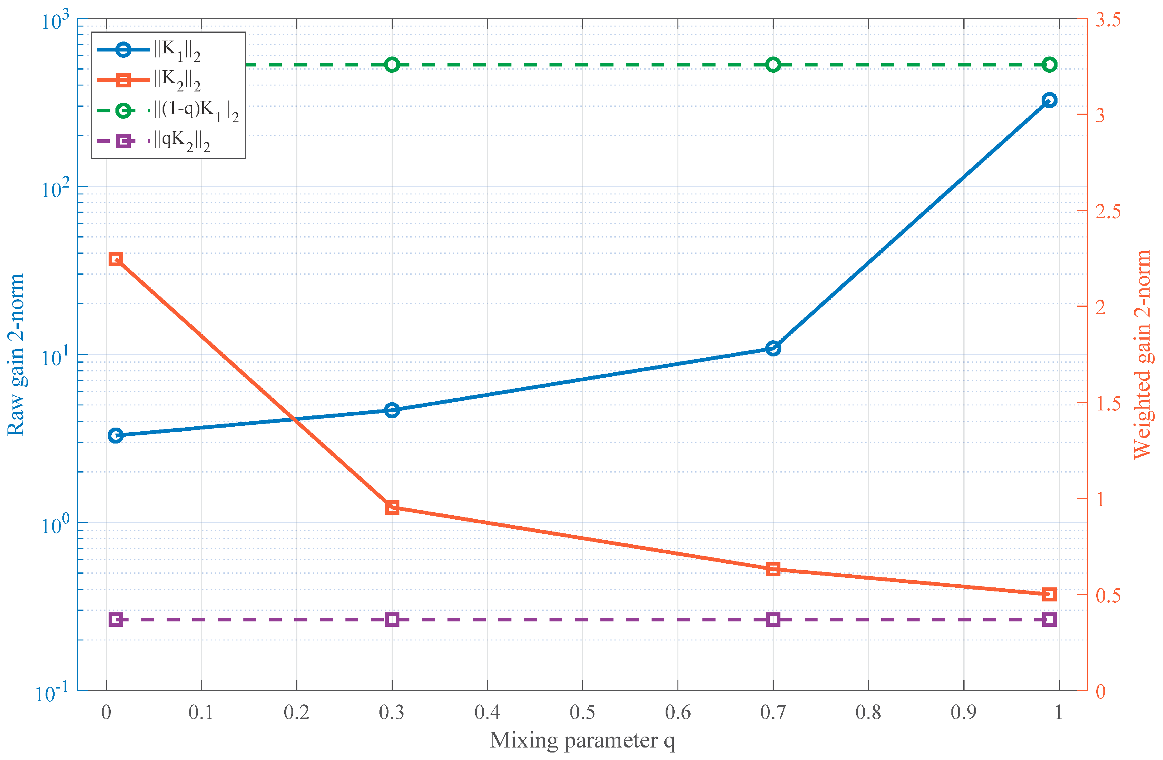
Let ${\overline{H}}_1\left(t\right)$ and ${\overline{H}}_2\left(t\right)$ be ${\overline{H}}_1\left(t\right)=\sin \left(t\right)I_3$ and ${\overline{H}}_2\left(t\right)=[\sin \left(t\right),\cos \left(t\right),\sin \left(t\right)]$, and set $q=0.5$. The state responses in Figure 3 show the followers approaching the leader. Tracking errors obtained with the nonfragile and conventional controllers are plotted in Figure 4 and Figure 5; both sets of curves tend to zero. The numerical behavior is consistent with the constant-delay result under randomly activated nonlinearities and uncertainty. Figure 6 displays the corresponding values of ${∥K_1∥}_2$, ${∥K_2∥}_2$, ${∥(1-q)K_1∥}_2$, and ${∥q{K}_2∥}_2$ as q changes.

Figure 3. State components of the leader and followers: (a) $x_{i1}$, (b) $x_{i2}$, and (c) $x_{i3}$.

Figure 4. Tracking-error components with the nonfragile controller: (a) $e_{i1}$, (b) $e_{i2}$, and (c) $e_{i3}$.

Figure 5. Tracking-error components with the conventional controller: (a) $e_{i1}$, (b) $e_{i2}$, and (c) $e_{i3}$.

Figure 6. Variation of ${∥K_1∥}_2$, ${∥K_2∥}_2$, ${∥(1-q)K_1∥}_2$ and ${∥q{K}_2∥}_2$ with q.

Example 2. 

Theorem 2 is examined with $x_{i1}$ and $x_{i2}$ selected from $[-1313]\times [-1313]$. In this case,

$$\begin{array}{c}\hfill \begin{array}{c}{\mathrm{\Gamma }}_1=\left[\begin{array}{cc}-1& 1.5\\ -1& 0\end{array}\right],{\mathrm{\Gamma }}_2=\left[\begin{array}{cc}0.5& -0.3\\ 0.3& -0.5\end{array}\right],B=\left[\begin{array}{c}1\\ 2\end{array}\right],\hfill \\ F_1=\mathrm{diag}\{0.01,0.01\},F_2=\mathrm{diag}\{0.01,-0.01\},E_1=\mathrm{diag}\{0.01,-0.01\},\hfill \\ F_3=\mathrm{diag}\{0.02,-0.03\},F_4=\mathrm{diag}\{0.02,0.02\},E_2=0.01.\hfill \end{array}\end{array}$$

The TVD is $\phi \left(t\right)=0.11{\sin }^2\left(t\right)+0.01$, for which $\widehat{\phi }=0.11$. Take ${\tilde{\epsilon }}_1=0.5$ and ${\tilde{\epsilon }}_2=0.7$; the other parameters are unchanged from Example 1.

Using feasp in MATLAB R2024a to test (26) produces

$$\begin{array}{c}\hfill \begin{array}{c}{\tilde{\sigma }}_1=0.5974,{\tilde{\sigma }}_2=0.5973,{\tilde{\delta }}_1=0.3286,{\tilde{\delta }}_2=0.0735,Q=0.1402\hfill \\ {\tilde{Q}}_1=\left[\begin{array}{cc}0.2482& -0.0540\\ -0.0540& 0.1672\end{array}\right],{\tilde{R}}_1={\left[\begin{array}{c}0.2612\\ 0.4782\end{array}\right]}^T,\hfill \\ {\tilde{M}}_1=\left[\begin{array}{cc}0.2017& -0.0037\\ -0.0037& 0.3008\end{array}\right],{\tilde{R}}_2={\left[\begin{array}{c}0.0343\\ -0.0454\end{array}\right]}^T.\hfill \end{array}\end{array}$$

Theorem 2 recovers $K_1$ and $K_2$ as

$$\begin{array}{c}\hfill K_1=\left[\begin{array}{cc}1.8629& 3.4100\end{array}\right],K_2=\left[\begin{array}{cc}0.2449& -0.3239\end{array}\right].\end{array}$$

The computed residual ${∥BQ-{\tilde{Q}}_{1}B∥}_2$ and maximum eigenvalue of $\mathrm{\Theta }$ satisfy

$$\begin{array}{c}\hfill {∥BQ-{\tilde{Q}}_{1}B∥}_2=1.9065\times {10}^{-5},{\lambda }_{\max }\left(\mathrm{\Theta }\right)=-0.0047.\end{array}$$

The functions $f\left(x_i(t-{\phi }_1)\right)$ and $g\left(x_i\left(t\right)\right)$ used here are

$$\begin{array}{c}\hfill \begin{array}{c}f\left(x_i(t-\phi \left(t\right))\right)={[0.5\sin \left(x_{i1}(t-\phi \left(t\right))\right),0.5\sin \left(x_{i2}(t-\phi \left(t\right))\right)]}^T,\hfill \\ g\left(x_i\left(t\right)\right)={[0.2\sin \left(x_{i1}\left(t\right)\right),0.2\sin \left(x_{i2}\left(t\right)\right)]}^T.\hfill \end{array}\end{array}$$

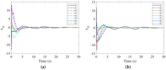
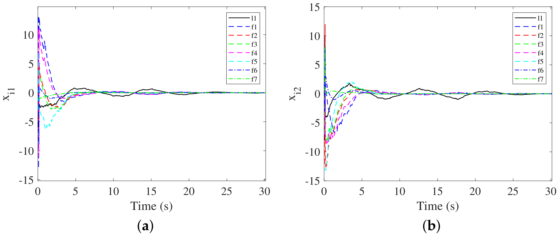
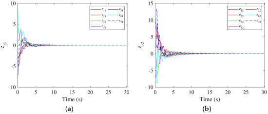
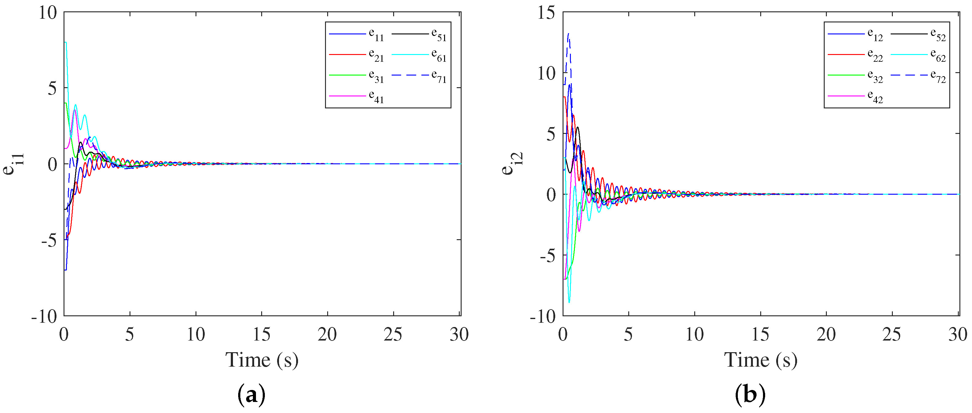
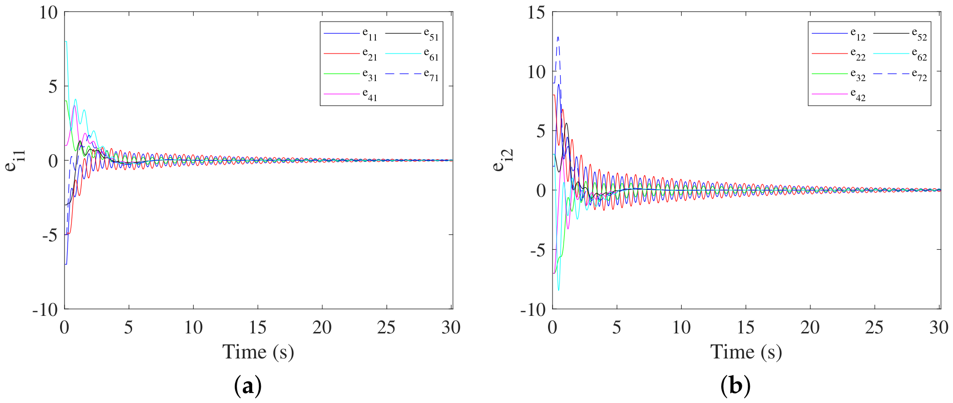
Let ${\overline{H}}_1\left(t\right)$ and ${\overline{H}}_2\left(t\right)$ be ${\overline{H}}_1\left(t\right)=\sin \left(t\right)I_2$ and ${\overline{H}}_2\left(t\right)=[\sin \left(t\right),\cos \left(t\right)]$, and set $q=0.5$. Figure 7 presents the agent states. In Figure 8 and Figure 9, every tracking-error curve approaches zero; this behavior supports the result with random nonlinearities and uncertainty.

Figure 7. Leader/follower state components: (a) $x_{i1}$ and (b) $x_{i2}$.

Figure 8. Tracking-error components with the nonfragile controller: (a) $e_{i1}$ and (b) $e_{i2}$.

Figure 9. Tracking-error components with the conventional controller: (a) $e_{i1}$ and (b) $e_{i2}$.

5. Conclusions

This work has investigated nonfragile stochastic tracking in delayed high-order MASs whose Lipschitz nonlinear dynamics exchange information over a directed graph. Randomly activated nonlinearities and plant uncertainty are modeled separately from diffusion noise. The distributed controller combines current and delayed state information under TVDs. Lyapunov analysis and matrix transformations lead to LMI-based stability criteria and computable controller gains. Two simulation studies support the theoretical conclusions. A natural extension is nonfragile stochastic tracking for delayed high-order MASs under switching topologies.

References

- Wang, P.; Wen, G.; Yu, W.; Huang, T.; Yu, X. An adaptive continuous approach to consensus tracking of nonlinear multiagent systems with a nonautonomous leader. IEEE Trans. Syst. Man Cybern. Syst. 2023, 53, 4684–4695. [Google Scholar] [CrossRef] [Scilit]
- Liu, Z.; Guo, M.; Li, Z. Time minimization and online synchronization for multi-agent systems under collaborative temporal logic tasks. Automatica 2024, 159, 111377. [Google Scholar] [CrossRef] [Scilit]
- Ye, P.; Shan, Q.; Li, T.; Chen, C.P. Practical time-varying formation-containment tracking for nonlinear multi-agent systems with general noise. J. Frankl. Inst. 2024, 361, 106822. [Google Scholar] [CrossRef] [Scilit]
- Xing, Y.; He, X.; Li, X. Disturbance observer-based event-triggered impulsive control for nonlinear systems with unknown external disturbances. Math. Comput. Simul. 2025, 227, 263–271. [Google Scholar] [CrossRef] [Scilit]
- Liu, Y.; Dong, X.; Zio, E.; Cui, Y. Event-triggered multiple leaders formation tracking for networked swarm system with resilience to noncooperative nodes. IEEE Trans. Cybern. 2025, 55, 4136–4144. [Google Scholar] [CrossRef] [Scilit] [PubMed]
- Zhou, T. H∞ containment control of multi-agent systems with mixed time-varying delays and exogenous disturbances via observer-based output feedback. Asian J. Control 2026, 28, 2108–2118. [Google Scholar] [CrossRef] [Scilit]
- Fang, X.; Xie, L.; Dimarogonas, D.V. Simultaneous distributed localization and formation tracking control via matrix-weighted position constraints. Automatica 2025, 175, 112188. [Google Scholar] [CrossRef] [Scilit]
- Xu, L.; Su, Y.; Cai, H. Event-triggered consensus of multiple nonholonomic mobile robots. Automatica 2025, 174, 112156. [Google Scholar] [CrossRef] [Scilit]
- Aghajari, H.A.; Niknam, T.; Shasadeghi, M.; Sharifhosseini, S.; Taabodi, M.; Sheybani, E.; Javidi, G.; Pourbehzadi, M. Analyzing complexities of integrating renewable energy sources into smart grid: A comprehensive review. Appl. Energy 2025, 383, 125317. [Google Scholar] [CrossRef] [Scilit]
- Liu, X.; Wang, Z.; Xing, L.; Wang, Y.; Zhang, C. Distributed current sharing and voltage regulation control for DC microgrids withgrid-forming and grid-feeding converters. Sci. China Inf. Sci. 2025, 55, 2622–2636. [Google Scholar] [CrossRef] [Scilit]
- Ma, L.; Wang, Z.; Han, Q.; Liu, Y. Consensus control of stochastic multi-agent systems: A survey. Sci. China Inf. Sci. 2017, 60, 120201. [Google Scholar] [CrossRef] [Scilit]
- Niu, X.; Liu, Y.; Li, F. Consensus via time-varying feedback for uncertain stochastic nonlinear multiagent systems. IEEE Trans. Cybern. 2019, 49, 1536–1544. [Google Scholar] [CrossRef] [PubMed]
- Li, M.; Wu, Z.; Deng, F.; Guo, B. Active disturbance rejection control to consensus of second-order stochastic multiagent systems. IEEE Trans. Control Netw. Syst. 2023, 10, 993–1004. [Google Scholar] [CrossRef] [Scilit]
- Sheng, L.; Ma, P.; Gao, M. H∞ consensus control with spectrum constraints for stochastic multi-agent systems subject to (x, u, v)-dependent noises. Appl. Math. Comput. 2019, 362, 124560. [Google Scholar] [CrossRef] [Scilit]
- Li, B.; Wen, G.; Peng, Z.; Huang, T.; Rahmani, A. Fully distributed consensus tracking of stochastic nonlinear multiagent systems with markovian switching topologies via intermittent control. IEEE Trans. Syst. Man Cybern. Syst. 2022, 52, 3200–3209. [Google Scholar] [CrossRef] [Scilit]
- Gu, H.; Liu, K.; Lü, J.; Ren, Z. Consensus of stochastic dynamical multiagent systems in directed networks via pi protocols. IEEE Trans. Syst. Man Cybern. Syst. 2022, 33, 6417–6428. [Google Scholar] [CrossRef] [Scilit] [PubMed]
- Li, K.; Li, Y. Adaptive NN optimal consensus fault-tolerant control for stochastic nonlinear multiagent systems. IEEE Trans. Neural Netw. Learn. Syst. 2023, 34, 947–957. [Google Scholar] [CrossRef] [Scilit] [PubMed]
- Wei, B.; Tian, E.; Gu, Z.; Zhai, J.; Liang, D. Quasi-consensus control for stochastic multiagent systems: When energy harvesting constraints meet multimodal FDI attacks. IEEE Trans. Cybern. 2024, 54, 1755–1767. [Google Scholar] [CrossRef] [Scilit] [PubMed]
- Li, Y.; Liu, L.; Hua, C.; Feng, G. Event-triggered/self-triggered leader-following control of stochastic nonlinear multiagent systems using high-gain method. IEEE Trans. Cybern. 2021, 51, 2969–2978. [Google Scholar] [CrossRef] [Scilit]
- Li, K.; Li, Y. Fuzzy adaptive optimal consensus fault-tolerant control for stochastic nonlinear multiagent systems. IEEE Trans. Fuzzy Syst. 2022, 30, 2870–2885. [Google Scholar] [CrossRef] [Scilit]
- Wang, J.; Wen, G.; Duan, Z.; Hu, Y.; He, W. Distributed H∞ robust control of multiagent systems with uncertain parameters: Performance-region-based approach. IEEE Trans. Syst. Man Cybern. Syst. 2022, 52, 2888–2898. [Google Scholar] [CrossRef] [Scilit]
- Wu, T.; Hu, J.; Chen, D. Non-fragile consensus control for nonlinear multi-agent systems with uniform quantizations and deception attacks via output feedback approach. Nonlinear Dyn. 2019, 96, 243–255. [Google Scholar] [CrossRef] [Scilit]
- Yang, Y.; He, Y. Non-fragile observer-based robust control for uncertain systems via aperiodically intermittent control. Inf. Sci. 2021, 573, 239–261. [Google Scholar] [CrossRef] [Scilit]
- Han, S.; Zhong, Q.; Wang, Y.; Shi, K.; Zhong, S. Nonfragile consensus of nonlinear multiagent systems with intrinsic delays via aperiodic memory sampled-data control. Int. J. Robust Nonlinear Control 2022, 32, 5164–5183. [Google Scholar] [CrossRef] [Scilit]
- Stephen, A.; Rajakopal, K.; Raja, R.; Srinidhi, A.; Thamilmaran, K.; Agarwal, R.P. Non-fragile reliable control for multi-agent systems with actuator faults using an improved LK functional. Nonlinear Dyn. 2025, 113, 6645–6669. [Google Scholar] [CrossRef] [Scilit]
- Hu, M.; Guo, L.; Hu, A.; Yang, Y. Leader-following consensus of linear multi-agent systems with randomly occurring nonlinearities and uncertainties and stochastic disturbances. Neurocomputing 2015, 149, 884–890. [Google Scholar] [CrossRef] [Scilit]
- Yuan, Y.; Wang, Z.; Zhang, P.; Dong, H. Nonfragile near-optimal control of stochastic time-varying multiagent systems with control-and state-dependent noises. IEEE Trans. Cybern. 2019, 49, 2605–2617. [Google Scholar] [CrossRef] [Scilit] [PubMed]
- Xiao, G.; Wang, J.; Meng, D. Adaptive finite-time consensus for stochastic multiagent systems with uncertain actuator faults. IEEE Trans. Control Netw. Syst. 2023, 10, 1899–1912. [Google Scholar] [CrossRef] [Scilit]
- Li, K.; Hua, C.; You, X.; Ahn, C.K. Leader-following consensus control for uncertain feedforward stochastic nonlinear multiagent systems. IEEE Trans. Neural Netw. Learn. Syst. 2023, 34, 1049–1057. [Google Scholar] [CrossRef] [Scilit]
- Yu, L.; Wang, Z.; Liu, Y.; Xue, C. Sampled-data nonfragile bipartite tracking consensus for nonlinear multiagent systems: Dealing with denial-of-service attacks. IEEE Trans. Syst. Man Cybern. Syst. 2025, 55, 1202–1214. [Google Scholar] [CrossRef] [Scilit]
- Jiang, X.; Xia, G.; Feng, Z.; Jing, X. Distributed sampled-data nonfragile consensus filtering over sensor networks with topology switching and transmission delay. IEEE/ASME Trans. Mechatron. 2022, 27, 1379–1390. [Google Scholar] [CrossRef] [Scilit]
- Zhang, K.; Zhou, B.; Duan, G. Leader-following consensus of multi-agent systems with time delays by fully distributed protocols. Syst. Control Lett. 2023, 178, 105582. [Google Scholar] [CrossRef] [Scilit]
- Wu, X.; Tang, Y.; Zhang, W. Stability analysis of stochastic delayed systems with an application to multi-agent systems. IEEE Trans. Autom. Control 2016, 61, 4143–4149. [Google Scholar] [CrossRef] [Scilit]
- Zhou, J.; Park, J.H.; Ma, Q. Non-fragile observer-based H∞ control for stochastic time-delay systems. Appl. Math. Comput. 2016, 291, 69–83. [Google Scholar] [CrossRef] [Scilit]
- Zhou, J.; Sang, C.; Li, X.; Fang, M.; Wang, Z. H∞ consensus for nonlinear stochastic multi-agent systems with time delay. Appl. Math. Comput. 2018, 325, 41–58. [Google Scholar] [CrossRef] [Scilit]
- Huang, X.; Liu, Y.; Wang, Y.; Zhou, J.; Fang, M.; Wang, Z. L2-L∞ consensus of stochastic delayed multi-agent systems with adt switching interaction topologies. Appl. Math. Comput. 2020, 368, 124800. [Google Scholar] [CrossRef] [Scilit]
- Kaviarasan, B.; Kwon, O.; Park, M.J.; Sakthivel, R. Stochastic faulty estimator-based non-fragile tracking controller for multi-agent systems with communication delay. Appl. Math. Comput. 2021, 392, 125704. [Google Scholar] [CrossRef] [Scilit]
- Kang, L.; Ji, Z.; Liu, Y.; Lin, C. Consensus of stochastic multi-agent systems with time-delay and Markov jump. Int. J. Syst. Sci. 2024, 55, 1959–1979. [Google Scholar] [CrossRef] [Scilit]
- Chen, L.; Liu, C.; Chu, Z.; Lopes, A.; Chen, Y. Leader-follower weighted consensus of nonlinear fractional-order multiagent systems using current and time delay state information. IEEE Trans. Syst. Man Cybern. Syst. 2024, 54, 5814–5823. [Google Scholar] [CrossRef] [Scilit]
- Mesbahi, M.; Egerstedt, M. Graph Theoretic Methods in Multiagent Networks; Princeton University Press: Princeton, NJ, USA, 2010. [Google Scholar]
- Wang, Z.; Yang, F.; Ho, D.W.; Liu, X. Robust H∞ control for networked systems with random packet losses. IEEE Trans. Syst. Man Cybern. Part B 2007, 37, 916–924. [Google Scholar] [CrossRef] [Scilit] [PubMed]
- Zhou, T.; Liu, C.; Wang, W. Nonfragile robust H∞ containment control for multi-agent systems with a time-varying delay. J. Frankl. Inst. 2024, 361, 106732. [Google Scholar] [CrossRef] [Scilit]
- Shen, B.; Wang, Z.; Liu, X. Sampled-data synchronization control of dynamical networks with stochastic sampling. IEEE Trans. Autom. Control 2012, 57, 2644–2650. [Google Scholar] [CrossRef] [Scilit]
- Xu, S.; Chen, T. Robust H∞ control for uncertain stochastic systems with state delay. IEEE Trans. Autom. Control 2002, 47, 2089–2094. [Google Scholar] [CrossRef] [Scilit]
Disclaimer/Publisher’s Note: The statements, opinions and data contained in all publications are solely those of the individual author(s) and contributor(s) and not of MDPI and/or the editor(s). MDPI and/or the editor(s) disclaim responsibility for any injury to people or property resulting from any ideas, methods, instructions or products referred to in the content. |
© 2026 by the authors. Licensee MDPI, Basel, Switzerland. This article is an open access article distributed under the terms and conditions of the Creative Commons Attribution (CC BY) license.