Article

An Efficient Iterative Method for the Analysis of Electrical Circuits with Nonlinear Inductive Elements

by
Claudiu Tufan
,
Alexandru Gabriel Gheorghe
* and
George Marian Vasilescu
Electrical Engineering Faculty, National University of Science and Technology POLITEHNICA Bucharest, 060042 Bucharest, Romania
*
Author to whom correspondence should be addressed.
Axioms 2026, 15(8), 621; https://doi.org/10.3390/axioms15080621
Submission received: 15 July 2026 / Revised: 14 August 2026 / Accepted: 18 August 2026 / Published: 20 August 2026
(This article belongs to the Special Issue Advances in Nonlinear Analysis and Numerical Modeling)

Abstract

This paper proposes and analyzes a modified version of the Hănțilă Method (HM) for solving electrical circuits with nonlinear inductive elements. The method replaces the nonlinear inductor with a generator comprising a nonlinear source and a linear impedance. The value of the nonlinear source is determined by defining a Picard–Banach fixed-point sequence that converges to the solution. This approach transfers the nonlinearity from the inductance to the generator’s source. The resulting circuit consists of linear and nonlinear sources and only linear components. It is solved in the harmonic domain using classical theorems and algorithms. A comparative analysis is performed on an RL circuit (a transformer primary winding at no-load). Both accuracy and computational effort are evaluated. The proposed iterative method is compared against steady-state time-domain transient analysis and frequency-domain approaches (Harmonic Balance Method) implemented in commercial software. This method is particularly suitable for analyzing circuits with nonlinear inductive components, such as iron-core coils and equivalent circuits for electrical machines.

1. Introduction

The world is undergoing a period of technological and economic transformations driving accelerated growth in electrical energy consumption. This pace is sustained by the expansion of digital infrastructure, particularly in data centers, including those dedicated to artificial intelligence. Efforts are being made to meet this growing demand through renewable energy production [1,2,3]. Large battery storage capacities are being developed to balance the load curve. However, the proliferation of power electronics and nonlinear circuit elements (NLE) introduces major challenges related to grid stability and power quality [4,5,6,7,8,9,10]. In this context, the use of efficient methods for modeling, simulating, and solving nonlinear electrical circuits and networks is becoming increasingly important [11].
Analytical methods are difficult to apply due to mathematical intractability in nonlinear systems. Consequently, their use is restricted to simple topologies. In such scenarios, numerical methods are far more suitable [12,13,14,15]. For solving systems of nonlinear equations, iterative methods are significantly more efficient than direct exhaustive search approaches. These methods construct sequences that converge to the solution, considerably reducing computation time and effort.
A well-recognized approach for solving engineering problems with nonlinearities is the Hănțilă method (HM). This method was successfully developed to solve electromagnetic field and eddy current problems in nonlinear media [16,17,18,19,20,21]. It has also been applied to analyze electrical circuits with resistive nonlinear elements (RNLE) under periodic steady-state conditions [22,23,24,25,26,27]. HM efficiently solves three-phase circuits, including those containing controlled-switching NLEs (thyristors), even under challenging computational conditions [24,25,26,27]. The primary advantages of this method are its reduced computational time and effort. Additionally, it ensures highly efficient memory usage. The mathematical convergence of HM is guaranteed and formally proven. Finally, the method allows for the analysis of a large number of harmonics and sampling points [23,24,25,26,27].
Originally developed for nonlinear electromagnetic field and eddy current problems [16,17,18,19,20,21], HM is based on decoupling the nonlinear material characteristics from the linear differential equations governing the field. In nonlinear continuous media, this separation is achieved by introducing a magnetic or electric polarization vector that incorporates the nonlinear material behavior. Consequently, the global boundary-value problem is formulated for a fixed, homogeneous linear medium excited by both external sources and the nonlinear polarization field acting as a fictitious source. At each iteration, the global field equations are solved for the linear medium (allowing for high computational efficiency through system matrix reuse), while the polarization vector is updated pointwise through local nonlinear constitutive corrections. This elegant transformation converts a complex nonlinear field problem into a convergent sequence of simple linear subproblems, each solved with high computational efficiency.
In this paper, we propose and analyze a modified version of HM to solve electrical circuits with nonlinear inductive elements (LNLE).
The HM version for LNLE (HML) is structurally similar—indeed almost identical—to HM for resistive nonlinear elements (HMR). A computational technique is employed where the variables used are no longer voltage and current. Instead, the algorithm operates on the inductor magnetic flux (in place of voltage) and the inductor current.
The illustrative example comparatively analyzes the results obtained for an RL circuit (a transformer primary winding at no-load) and the computational effort required by HML against classical circuit analysis approaches. These commercial software approaches include time-domain transient analysis (TR) run until periodic steady-state is reached, and frequency-domain Harmonic Balance (HB). The proposed method is useful for analyzing circuits with LNLE, as is the case with iron-core coils or equivalent circuits of electrical machines (transformers, motors, generators).

2. HML with Flux Correction of the Nonlinear Source

HML replaces the LNLE with an equivalent generator consisting of a nonlinear voltage source and a linear impedance. The value of the nonlinear source is determined by defining a Picard–Banach fixed-point iteration that converges to the solution. This approach transfers the nonlinearity from the inductance to the generator’s source. The linear impedance is selected based on the characteristic parameters of the LNLE to ensure the convergence of the algorithm.
The resulting circuit, containing linear and nonlinear sources and only linear passive components, is solved for each harmonic using classical circuit theorems and algorithms. The value of the generator’s nonlinear source is updated iteratively. This is the key computational advantage of HM: it does not attempt to solve a system of nonlinear equations directly. Instead, it solves a series of simple linear circuits, using the nonlinearity solely to correct the value of the source. Consequently, the computational effort is significantly reduced, and the solution is reached very rapidly.
The method has two dual variants: one with flux-correction and the other with current-correction of the nonlinear source value. In this paper, the flux-corrected variant is analyzed. The current-corrected variant will be addressed in a future paper.
In the case of flux-correction, the LNLE is replaced with a voltage generator. This generator consists of a nonlinear voltage source in series with a linear inductor. The value of the nonlinear source is iteratively corrected. To ensure the convergence of the algorithm, the inductance of the generator’s linear inductor is selected based on the parameters of the nonlinear inductor’s current-flux characteristic. During the iterations, the source voltage value is not directly corrected. Instead, the correction is applied to its associated magnetic flux. The construction of the Picard–Banach fixed-point iteration and the description of its constituent operators are detailed in the next subsections.
Next, the HML variant with flux-correction of the nonlinear source is analyzed. Although some of the equations and proofs are practically identical to those of HMR from [22,23,24,25,26,27], they are presented here again for the reader’s convenience.

2.1. The g Operator

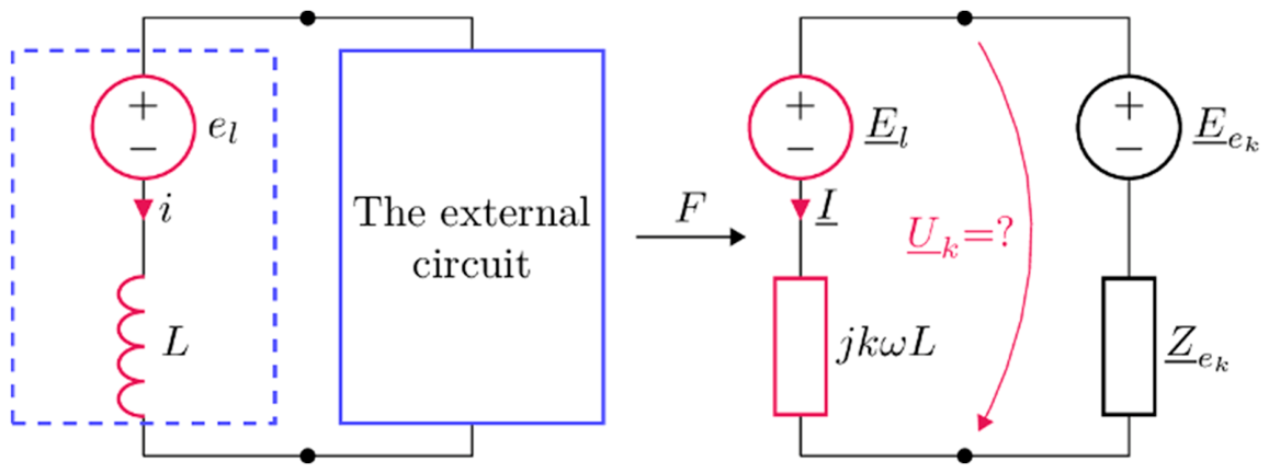
The LNLE is replaced with a voltage generator, as shown in Figure 1, where LNLE denotes the nonlinear coil inductance, which is defined by its current–flux characteristic. The circuit elements that have been replaced are marked in red, while the external circuit of the nonlinear coil is shown in blue. This generator comprises a nonlinear voltage source in series with a linear inductor L .
The nonlinear current-flux characteristic of the LNLE is described by the function
i = f ( ϕ ) ,
where f : R → R , i is the current through the LNLE, and ϕ is the magnetic flux.
From the constitutive equations of the circuit elements in Figure 1, the voltage across the terminals of the LNLE is obtained
u = L d i d t + e l .
The relationship between voltage and flux is given by Faraday’s law of electromagnetic induction:
u = d ϕ d t .
By substituting the voltage from (3) into Equation (2) and integrating with respect to time, the equation becomes
ϕ = L i + ϕ e ,
where ϕ e is the flux component associated with the nonlinear source e l . This component ϕ e satisfies Faraday’s law of electromagnetic induction, being related to the voltage by:
e l = d ϕ e d t .
To simplify the analysis, the initial conditions are assumed to be zero. For this reason, introducing an integration constant into the structure of Equation (4) is no longer necessary.
From a mathematical standpoint, Equation (4) is identical to the constitutive equation of the voltage generator from [22,23,24,25,26,27]:
u = R i + e .
Due to the mathematical identity between Equations (4) and (6), the proofs in this subchapter are similar to those in [22,23,24,25,26,27]. They are presented below to ensure a clear understanding of the algorithm and do not constitute a novel contribution. The calculation steps follow those in [22,23,24,25,26,27], except that voltage is replaced by magnetic flux and resistances are replaced by inductances.
Similarly to [22,23,24,25,26,27], the operator g is defined as
g ( ϕ ) = ϕ e = ϕ − L i = ϕ − L   f ( ϕ ) = ϕ ( 1 − L f ( ϕ ) ϕ ) ,
which maps ϕ to ϕ e in the time domain:
ϕ → g ϕ e .
For the final algorithm to converge, the g operator must be a contraction in the Hilbert space of periodic functions. g ( ϕ ) is a contraction if there exists a contraction factor θ g ∈ ( 0,1 ) such that:
g ( ϕ 1 ) − g ( ϕ 2 ) ≤   θ g ϕ 1 − ϕ 2   ∀   ϕ 1 ,   ϕ 2 .
The norm is defined in the Hilbert space of periodic functions with period T using the inner product with weight 1 L :
ϕ 1 , ϕ 2 1 / L = ∫ 0 T ϕ 1 ϕ 2 L d t .
It can be shown that for g to be a contraction, it is sufficient for f to be Lipschitz continuous and uniformly monotonic [22,23,24,25,26,27], satisfying:
S u p ϕ 1 , ϕ 2 ∈ R f ( ϕ 1 ) − f ϕ 2 ϕ 1   − ϕ 2   = Λ ≝ 1 L m i n > 0 ,     ϕ 1 ≠ ϕ 2 ,
I n f ϕ 1 , ϕ 2 ∈ R f ( ϕ 1 ) − f ϕ 2 ϕ 1   − ϕ 2   = λ ≝ 1 L m a x > 0 ,     ϕ 1 ≠ ϕ 2 .
If Equations (10)–(12) hold for any time instant within a period T , then the following inequalities also hold:
0 < 1 L m a x ≝ λ ≤   f ( ϕ 1 ) − f ϕ 2 ϕ 1   − ϕ 2     ≤ Λ ≝ 1 L m i n ∀   ϕ 1 , ϕ 2   w i t h   ϕ 1 ≠ ϕ 2 .
f denotes the current-flux characteristic of the LNLE and satisfies the inequalities in (11)–(13). The NLEs considered here have a finite operating range of fluxes and currents. Consequently, the ratio of the variations in these two quantities is also finite. The value of this ratio falls within two well-defined limits. Nonlinear characteristics exhibiting hysteresis-type jumps or discontinuities are not analyzed in this paper. Addressing these remains a topic for future research. In this study, the analysis is limited to nonlinear characteristics with a narrow hysteresis loop. These can be approximated by the initial magnetization curve, which satisfies conditions (11)–(13). Representative examples include coils with a ferromagnetic core and the primary winding of a transformer operating under no-load conditions.
In real ferromagnetic components, the relationship between magnetic flux and current is nonlinear, multivalued, and path-dependent, involving major and minor hysteresis loops. However, for a broad class of practical engineering applications (particularly those involving soft magnetic materials characterized by very narrow hysteresis loops), the difference between the ascending and descending branches has a negligible effect on terminal voltage and current waveforms or harmonic spectra. In such cases, adopting a single-valued monotonic approximation (such as an anhysteretic or initial magnetization curve) can provide sufficient accuracy while maintaining practical engineering relevance.
Furthermore, multivalued hysteresis modeling is frequently bypassed in practical simulation workflows because existing hysteresis formulations may exhibit significant discrepancies when compared with experimental measurements.
In this work, the foundational mathematical formulation and theoretical convergence analysis of the HML framework are established assuming single-valued continuous magnetic characteristics. Multivalued memory operators are explicitly excluded from the present scope. To our knowledge, existing hysteresis models do not yet provide a universally satisfactory level of physical fidelity over a broad range of operating conditions. If a physically accurate, high-fidelity model becomes available, its mathematical structure and compatibility with the HML framework will be investigated in future work.
Equations (7) and (9) yield:
ϕ 1 − L f ( ϕ 1 ) − ( ϕ 2   − L f ϕ 2 )   ≤ θ g ϕ 1 − ϕ 2   ∀   ϕ 1 , ϕ 2 .
Considering that f : R → R , it follows that:
1 − L f ( ϕ 1 ) − f ϕ 2 ϕ 1   − ϕ 2   = 1 − L ∆ L 12 ≤ θ g < 1     with     ∆ L 12 ∈ [ L m i n , L m a x ] .
Equation (15) holds if:
L ∈ ( 0 ,   2 L m i n ) .
Equation (16) represents the sufficient condition for the g operator to be a contraction. This property ensures the convergence of the algorithm.
From (15), the contraction factor can be calculated as
θ g = M a x 1 − L L m a x , L L m i n − 1 .
Similarly to [22,23,24,25,26,27], the value of θ g can be optimized by setting the two terms in (17) equal, yielding:
L o p t = 2 L m i n L m a x L m i n + L m a x ,
which leads to the minimum contraction factor:
θ g o p t = L m a x − L m i n L m a x + L m i n .
Using L o p t does not guarantee the shortest computation time. However, this behavior is confirmed in most cases. The computation time also depends on how the choice of L affects the evaluation of the operator h , an aspect analyzed in the next subsection. Nevertheless, it can be mathematically proven that choosing L within the interval L m i n ,   2 L m i n ensures faster convergence than selecting it from the interval ( 0 ,   L m i n . In the illustrative example, the efficiency of the method is comparatively analyzed under two scenarios: L = L o p t and L = L m i n .
The operator g is defined to map ϕ to ϕ e , ensuring that it is a contraction. Both the operator g and its coefficients can be precomputed prior to the start of the iterative process. This operator is applied at each iteration to perform the correction according to the nonlinear characteristic. The evaluation is carried out in the time domain and requires minimal computational effort.

2.2. The h Operator

In the previous subsection, the LNLE was replaced by a voltage generator consisting of a nonlinear voltage source in series with a linear inductor of value L . The rest of the circuit is connected across the terminals of this generator, as shown in Figure 2.
If the initial circuit contains only a single nonlinear element (NLE), the external circuit will be linear. If multiple NLEs are present in the initial circuit, the substitution described in the previous subsection is performed for all NLEs. In this case, the external circuit will consist of linear and nonlinear sources and linear circuit elements. In either scenario, an equivalent generator comprising a linear voltage source and an internal impedance can be calculated across the generator terminals in the frequency domain using a Fourier series expansion for each harmonic [22,23,24,25,26,27]. Consequently, a linear circuit must be solved in the complex domain for each harmonic. This is straightforwardly accomplished by applying Kirchhoff’s laws. For each harmonic k , two parallel-connected voltage generators are obtained. The objective is to determine the voltage U _ k across the terminals of each nonlinear generator for each harmonic k
U _ k = E _ l k Z _ e k + E _ e k × j k ω L Z _ e k + j k ω L = E _ l k Z _ e k Z _ e k + j k ω L + E _ e k j k ω L Z _ e k + j k ω L .
Because the HM replaces every nonlinear element with a linear component and a nonlinear source, the entire network becomes strictly linear at each iteration step. Consequently, for any harmonic k (regardless of the number of nonlinear elements present), the external circuit connected across the terminals of any specific element can always be reduced to a single Thévenin or Norton equivalent circuit via standard linear network reduction techniques (superposition and Kirchhoff’s laws).
If there are no other NLEs in the circuit, E _ e k will be nonzero only for the frequencies of the power sources in the circuit. If the power sources operate at a single frequency, E _ e k will be nonzero only for the fundamental frequency.
In (20), the voltages are replaced by the fluxes, following the same procedure as in (3) and (5). In the complex domain, the time derivative operation for the k -th harmonic transforms into multiplication by j k ω . Thus, for each harmonic k , the equation relating ϕ e _ k to ϕ _ k is obtained:
ϕ _ k = ϕ e _ k Z _ e k Z _ e k + j k ω L + E _ e k L Z _ e k + j k ω L ≝ h k ( ϕ e _ k ) .
h k ( ϕ e _ k ) is required to be nonexpansive for each harmonic k , which means that:
h k ( ϕ e _ k 1 ) − h k ( ϕ e _ k 2 ) ≤   ϕ e _ k 1 − ϕ e _ k 2   ∀   ϕ e _ k 1 ,   ϕ e _ k 2 .
The norm in (22) is defined in the space of complex vectors ϕ _ as ϕ _ 1 L 2 = 1 L ∑ k = 1 K ϕ _ k · ϕ _ k ¯ , where k is the harmonic order, K is the total number of harmonics used for the Fourier series truncation, and ϕ _ k ¯ denotes the complex conjugate of ϕ _ k .
Substituting (21) into (22) and taking into account that the analysis is performed in the complex domain yields:
ϕ e _ k 1 − ϕ e _ k 2 Z _ e k Z _ e k + j k ω L ≤   ϕ e _ k 1 − ϕ e _ k 2   ∀   ϕ e _ k 1 ,   ϕ e _ k 2 .
This implies that the following condition must be satisfied:
Z _ e k Z _ e k + j k ω L ≤ 1 .
Given that Z _ e k is a complex impedance with
Z _ e k = R k + j X k .
Substituting (25) into (24) and calculating the magnitudes, it follows that (22)–(24) hold true if
R k 2 + X k 2 ≤ R k 2 + ( X k + k ω L ) 2 ,
0 ≤ 2 X k k ω L + ( k ω L ) 2 ,
X k ≥ − k ω L 2 .
If (28) is satisfied for each harmonic k , then h k is non-expansive for all k , and consequently, h is non-expansive with h ≤   1 .
Here, a significant difference from HMR arises. For HMR, h k is always non-expansive. This results unconditionally from the connection topology of the nonlinear voltage generator with the rest of the circuit. In the HML case, h k is not inherently non-expansive. It is guaranteed to be non-expansive if the external circuit contains only resistive and inductive elements (linear and/or nonlinear). However, convergence issues can occur if the circuit contains capacitors (even linear ones). The critical factor is the value of the equivalent capacitive reactance for each harmonic at the LNLE terminals and whether this value satisfies (28).
Power transmission and distribution networks are designed and operated to maintain an overall inductive character. For long underground cables, their significant capacitive reactance must be compensated locally to prevent the Ferranti effect. The Ferranti effect represents the voltage rise phenomenon at the receiving end of a long, uncompensated power line operating at no-load or under light-load conditions. Power distribution operators impose financial penalties for capacitive reactive power injected into the grid. Industrial consumers are heavily billed for this uncompensated capacitive energy. Therefore, HML should not encounter issues with condition (28) in power network analysis due to the predominantly inductive nature of these systems.
On the other hand, significant capacitive reactances and resonance phenomena occur frequently in electronic circuits. Analyzing such circuits using HML could raise convergence issues. This happens if the equivalent capacitive reactance violates the limit imposed by condition (28).
Several solutions could extend the allowable range for X k . The values of the h k coefficients can be quickly computed from the beginning. It is easy to detect if h k is not non-expansive on certain harmonics. Part of the equivalent capacitive reactance could be transferred by modifying the nonlinear current–flux characteristic to satisfy (28). This solution is similar to the one proposed in [25], where the nonlinear current–voltage characteristic was modified by transferring part of the external circuit’s equivalent resistance. We aim to develop and analyze such a solution in a future paper.
From (24), it is observed that a larger chosen value for L , as close as possible to 2 L m i n , is beneficial. This allows for a higher capacitive reactance value. Furthermore, choosing a larger value of L ensures smaller h k coefficients for the harmonics, leading to better convergence of the algorithm.
Usually, LNLEs do not exhibit severe nonlinearities. The L m a x / L m i n ratio is relatively small, typically ranging between 2 and 20. Rarely, it can reach 50 or 100 in the case of special materials with very high initial permeability. These values are considerably smaller than those of RNLEs, where the R m a x / R m i n ratio usually reaches values of 105 or even 1012. A smaller ratio leads to a very good contraction factor for g . In certain situations, this could compensate for a slightly expansive h k on certain harmonics. This corresponds to values of Z _ e k Z _ e k + j k ω L slightly greater than 1. We aim to conduct such an analysis in a future paper.
It should be mentioned that this work aims to develop and apply HML exclusively to electrical circuits that admit a unique steady-state solution (sinusoidal or non-sinusoidal). Circuits without a solution or those with chaotic and unpredictable behavior are excluded from our scope. Such circuits are characterized by the strict monotonicity and passivity of their component elements. This ensures the asymptotic stability of the operating regime and the global convergence of the iterative algorithms.
The operator h maps the complex value ϕ e _ to ϕ _ in the frequency domain
ϕ e _   → h ϕ _ .
This operator has the components h k for each harmonic. If h k is non-expansive for all harmonics, then h is also non-expansive.
Similar to operator g , the h k coefficients can be computed at the beginning, before starting the iterative process. This operator is applied at each iteration to establish the connection with the external circuit. The evaluation is carried out in the frequency domain and requires reduced computational time and effort.

2.3. The HML Algorithm

In the previous subsections, the two operators, g and h , were defined.
The operator g maps ϕ to ϕ e in the time domain. It ensures the correction using the nonlinear current–flux characteristic. If (16) holds true, g is a contraction.
The operator h maps ϕ e _ to ϕ _ in the frequency domain. It establishes the connection with the external circuit at the terminals of the LNLE. If (28) is satisfied, h is non-expansive.
To define the algorithm, the operators F and F − 1 are also required. The operator F represents the Fourier series expansion and maps the time domain to the frequency domain. Conversely, F − 1 is the inverse operation of F , mapping the frequency domain back to the time domain. Due to truncation to a finite number of harmonics, F changes from a perfect isometry to a non-expansive operator [22,23,24,25,26,27]. On the other hand, F − 1 remains a perfect isometry and has a Lipschitz constant equal to 1.
With the operators defined above, the iterative solution algorithm from iteration n to iteration n + 1 is:
…   ϕ e ( n ) → F ϕ e _ ( n ) → h ϕ _ ( n ) → F − 1 ϕ ( n ) → g ϕ e ( n + 1 ) …   .
We have the contraction operator g , the non-expansive operators h and F , and the isometry F − 1 . The algorithm is a composition of these operators and converges in both the frequency and time domains. Convergence is guaranteed as long as (16) and (28) are satisfied.
From Figure 2 and Equation (23), for the DC component, the operator norm coefficient of h 0 is equal to 1, because inductors act as short circuits and capacitors as open circuits at DC. Even after harmonic truncation, the Lipschitz constant of h remains 1 if a DC component is present. Therefore, in the general case, the overall contraction factor of the iterative algorithm is strictly dictated by the contraction factor of operator g .
However, in the particular case where the nonlinear characteristic is symmetric with respect to the origin (an odd function), all even harmonics, including the DC component, are zero. In this scenario, if a unit norm coefficient no longer appears on any active harmonic, eliminating the even harmonics and truncating the series allows operator h to behave as a strict contraction. Such a case is analyzed in the illustrative example in Section 3, where explicit numerical values for the Lipschitz constants of operators h and g , as well as the resulting contraction factor of the algorithm, are provided.
The coefficients of the operators g and h can be computed from the beginning, and the application of these two operators is very fast. Applying the operators F and F − 1 is more time- and resource-consuming. However, if the number of harmonics used to truncate the Fourier series is below 100, the required computational time is also quite small. Furthermore, for both F and F − 1 , a portion of the coefficients can be precomputed.
Similar to [22,23,24,25,26,27], the error (distance) between two successive values of ϕ e _ at iteration n is defined as
ε ( n ) ≝ ϕ e _ ( n ) − ϕ e _ ( n − 1 ) .
The relative error is used as the stopping criterion for the iterations:
ε r ( n ) ≝ ε ( n ) e / j ω ,
where e is the value of the circuit’s voltage supply.
The algorithm starts from an initial value of ϕ e . The operators F , h , F − 1 , and g are applied sequentially in accordance with (30) until the desired value of ε r is reached. At this point, the iterations are stopped. The Picard–Banach sequence converges from any chosen value of ϕ e . If there is no preferred starting value, the default value is set to ϕ e = 0 .
Once the magnetic flux component associated with the nonlinear source, ϕ e _ , is computed with the desired accuracy, the voltage of the nonlinear source can be computed in the frequency domain, followed by the voltages and currents for all other circuit elements.
Given the similarity between HMR and HML, most of the acceleration techniques developed for HMR in [23,24,25,26,27] can also be adapted and applied to HML. However, to evaluate the intrinsic numerical stability and baseline convergence rate of the proposed algorithm, these acceleration schemes are deliberately not employed in the numerical examples presented in Section 3. Furthermore, while HML shares structural principles with the resistive voltage-current formulation, extending the framework to magnetic flux–current characteristics requires distinct operator mappings. In particular, a new non-expansiveness condition for operator h is established in this paper. Additionally, all theoretical derivations and convergence proofs have been fully detailed within this text to ensure the manuscript is completely self-contained and easy to follow.
In the case of electrical circuits with nonlinear capacitors, the construction of the algorithm and the proofs are similar. The condition for ensuring the non-expansiveness of the operator h is dual. The correction of the nonlinear source substituting the nonlinear capacitance is performed in terms of charge or voltage. We intend to analyze such a circuit in a future paper.

3. Illustrative Example

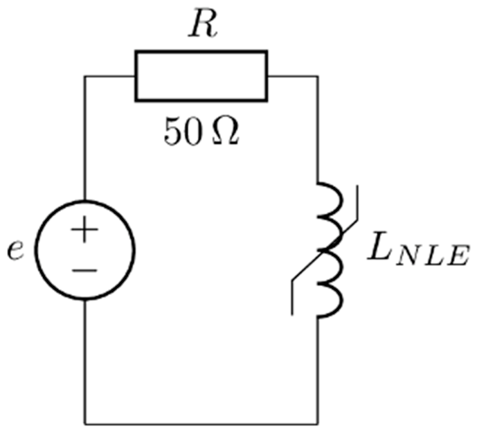
To evaluate the efficiency of the HML, the circuit shown in Figure 3 is analyzed. This circuit represents a transformer primary winding at no-load conditions connected to a voltage source. The results and computational effort are compared against ADS 2026 Update 1 [28] in both HB and TR modes, and LTspice Version 26.0.2 [29] in TR mode.
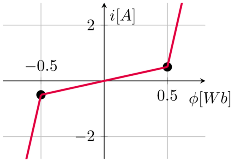
The circuit’s voltage supply e is sinusoidal, with an amplitude of 325 V and a frequency of 50 Hz. The resistance is 50 Ω. The nonlinear current–flux characteristic of the LNLE is shown in Figure 4.
A piecewise linear (PWL) model is employed for the LNLE. The branch inductances have the values L l o w = 0.05   H and L h i g h = 1   H , with a saturation current i s a t = 0.5   A and a saturation flux ϕ s a t = 0.5   W b , described by the equation
i ( ϕ ) = ϕ + ϕ s a t L l o w − i s a t       f o r         ϕ < − ϕ s a t ϕ L h i g h       f o r   − ϕ s a t ≤ ϕ ≤ ϕ s a t ϕ − ϕ s a t L l o w + i s a t     f o r         ϕ > ϕ s a t .
To keep the present paper concise, the current study analyzes a fundamental circuit containing a single nonlinear inductive element. However, the proposed HML framework can be extended to handle multiple nonlinear inductive elements, including mutual magnetic coupling, similar to the multi-element algorithm presented in [27]. Expanding the numerical validation to complex multi-element topologies (such as autotransformers and three-phase transformers) constitutes a primary objective for a series of future publications.
In this example, a three-segment PWL characteristic was selected as the benchmark nonlinearity. In numerical analysis and electromagnetic simulation tools (such as Finite Element Method software or circuit simulators), pointwise linear interpolation of discrete experimental data represents the de facto standard approach for defining B − H and flux-current characteristics. Furthermore, from a numerical perspective, PWL characteristics with sharp knee points introduce derivative discontinuities, making convergence significantly more challenging for iterative solvers than in the case of smooth, continuously differentiable analytical functions (e.g., hyperbolic tangent or arctan curves). The HML algorithm can be directly extended to multi-segment PWL representations or smooth analytical curves without altering its underlying mathematical formulation. Extended evaluations incorporating smooth functions and multi-segment curves will be addressed in future work.

3.1. Application of HML

For HML, the variant with flux correction of the nonlinear source is used. In accordance with Section 2.1, the LNLE is replaced by a voltage generator consisting of a nonlinear voltage source in series with a linear inductor L . The value of L must be chosen within the interval ( 0 ,   2 L m i n ) according to (16).
From (7) and (33), the g operator is obtained:
g ( ϕ ) = ϕ ( 1 − L L l o w ) − L ( ϕ s a t L l o w − i s a t )       f o r         ϕ < − ϕ s a t ϕ ( 1 − L L h i g h )       f o r     − ϕ s a t ≤ ϕ ≤ ϕ s a t ϕ ( 1 − L L l o w ) + L ( ϕ s a t L l o w − i s a t )     f o r         ϕ > ϕ s a t .
The simulation is performed for two values of L :   L = L o p t and L = L m i n . For the nonlinear characteristic shown in Figure 4, L m i n = L l o w and L m a x = L h i g h .
The Fourier series expansion is truncated to 9, 20, 40, and 100 harmonics plus the DC component (denoted in the sequel as 10, 21, 41, and 101). The signal was sampled at 32, 64, 128, and 256 sampling points, respectively.
The coefficient values for the operator h are computed according to (21). Except for the DC component, where its value is 1, the operator h k behaves as a contraction on all other harmonics, having a Lipschitz constant less than unity. Since the current-flux characteristic shown in Figure 4 and described by (33) is symmetric with respect to the origin, the coefficient of the DC component is practically irrelevant. Theoretically, the value of this component is zero.
Table 1 summarizes the magnitudes of coefficients and Lipschitz constants corresponding to operators g and h , as well as the overall algorithm contraction factor. Since the characteristic shown in Figure 4 and Equation (33) is an odd function, symmetric with respect to the origin, the spectrum contains no even harmonics. In this case, operator h behaves as a contraction. The overall algorithm contraction factor is obtained by multiplying the Lipschitz constants of the constituent operators, with the corresponding numerical values presented in Table 1. The results obtained in the illustrative example confirm the contraction of g and the non-expansiveness of h .
The algorithm was initialized with ϕ e = 0 . HML was executed in GNU Octave 6.2.0 [30] using software developed by the authors and based on the algorithm presented in Section 2. The program was run on a laptop equipped with a 2.3 GHz 8-core Intel Core i9 processor (9th Generation) and 16 GB of 2667 MHz DDR4 memory.
The algorithm was terminated upon reaching a relative error of 10−6, computed according to (32). The number of iterations and the required computation time in milliseconds are presented in Table 2.
It can be observed that utilizing L = L o p t is slightly more efficient than L = L m i n , resulting in fewer iterations and a slightly shorter computation time.
All reported calculation times in Table 2 represent the mean execution time evaluated over 10 consecutive runs under standard computing conditions. Because the proposed algorithm is strictly deterministic (initialized from a fixed zero state without stochastic or shooting-based initial guesses), the required number of iterations and floating-point operations remains identical across runs. The reported timing values serve as indicative metrics of computational effort, with minor OS-level scheduling variations across runs without extreme runtime outliers.
No acceleration techniques, such as those presented in [23,24,25,26,27], were employed. The only speedup was achieved through the choice of the L values.
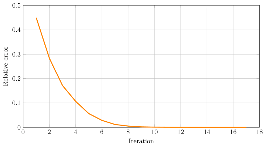
Several plots obtained from the simulations for 101 harmonics and 256 sampling points are presented below. Figure 5 illustrates the evolution plot of the relative error ε r ( n ) for L = L o p t .
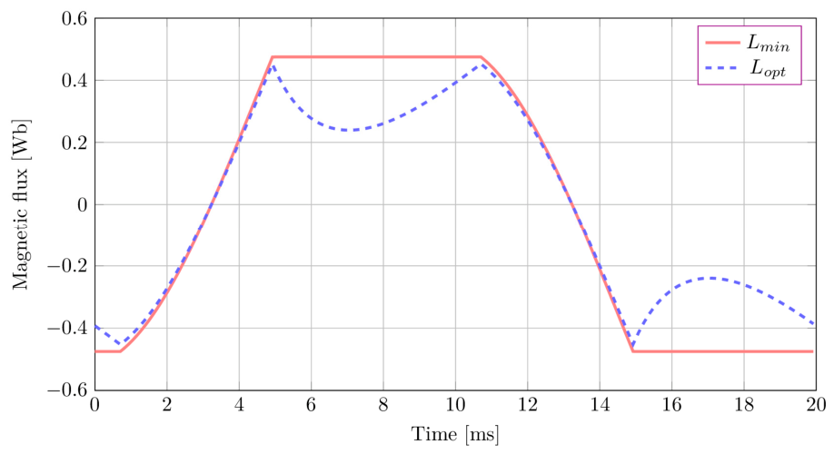
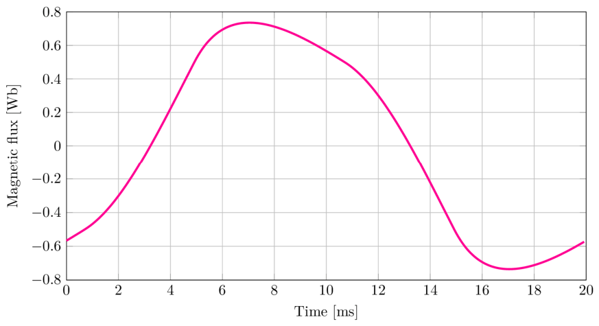
Figure 6 presents the flux component associated with the nonlinear source ϕ e obtained for the two analyzed cases, L = L o p t and L = L m i n . The difference between the two superimposed time-domain representations can be clearly observed. Figure 7 shows the time-domain magnetic flux ϕ of the LNLE.
The algorithm used for HML is based on a classical approach for calculating the operator F and F − 1 . The FFT and IFFT algorithms available in GNU Octave [30] were not utilized, thereby maintaining better accuracy. This approach allowed us to ensure that the lookup tables for the sine and cosine functions were mapped to the first quadrant. Furthermore, it offers greater flexibility in selecting the number of harmonics and the analyzed sampling points [23,24,25,26,27].
Depending on the desired accuracy and computation time, the number of harmonics and sampling points can be increased or decreased. In addition, the stopping criterion of the algorithm can also be modified.
To keep the present paper concise, the detailed numerical evaluation of strongly capacitive circuit topologies in which condition (28) is violated is reserved for future work. From a theoretical perspective, when condition (28) fails to hold, the HML algorithm loses its contraction property and becomes divergent, causing the error norm between consecutive iterations from (31) and (32) to grow rather than decay. A dedicated forthcoming study will thoroughly analyze these divergent regimes and introduce a targeted algorithmic remedy designed to guarantee numerical convergence even when condition (28) is breached.

3.2. Application of ADS HB and TR

In the ADS HB simulation, the same number of harmonics and sampling points as in HML was maintained. The following settings were used: Convergence mode: Robust, Linear solver: Direct, and Matrix Bandwidth: Robust. The obtained computation times and number of iterations are presented in Table 3.
The transient analysis in ADS can detect the moment when steady state is reached, which occurs at t = 70 ms for the circuit studied in this article. To obtain data over one period of the source and to compare the solution with those obtained with HML and ADS HB, the stop time was increased to Tstop = 100 ms.
In transient analysis, the time step can be chosen either automatically or by the user. To compare the computation time with that of HML and HB, the same number of samples per period was imposed as in the previously mentioned methods. The results are presented in Table 4.

3.3. Application of LTspice TR

In LTspice TR, the same number of sampling points as in HML and ADS TR was imposed. Similar to ADS TR, the steady-state regime was considered to begin with the fifth period of the signals. For the comparison in the following subsection, the period between 80 ms and 100 ms was used. The options modified trap, alternate, abstol = 1 p, reltol = 1 × 10⁻⁵, chgtol = 1 f, trtol = 7, plotwinsize = 0, and vntol = 1 × 10⁻⁷ were used. The computation times are presented in Table 5.

3.4. Comparative Study

It can be observed from Table 2, Table 3, Table 4 and Table 5 that the computation times of the HML are of the same order of magnitude as, and in certain cases even lower than, those achieved by commercial software. The times are comparable to those obtained with LTspice TR and significantly shorter than those obtained with ADS HB and TR. To provide a practical reference, execution times were recorded and compared alongside the iteration counts. Although a direct wall-clock CPU comparison between a custom Octave implementation and compiled commercial solvers is subject to inherent software-level asymmetries (such as GUI overhead, interpreted execution, and differences in multithreading), the reported runtimes serve as a useful order-of-magnitude benchmark. Notably, despite operating within an interpreted environment, the HML method achieves highly competitive execution times. This performance can be attributed to its fundamental algorithmic advantage: the linear system matrix is factorized only once at the initialization step, reducing each subsequent iteration to simple forward and backward substitutions, whereas conventional NR solvers require recalculating and refactorizing the Jacobian matrix at every iteration.
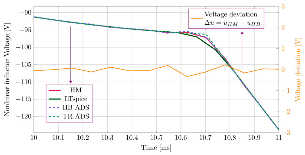
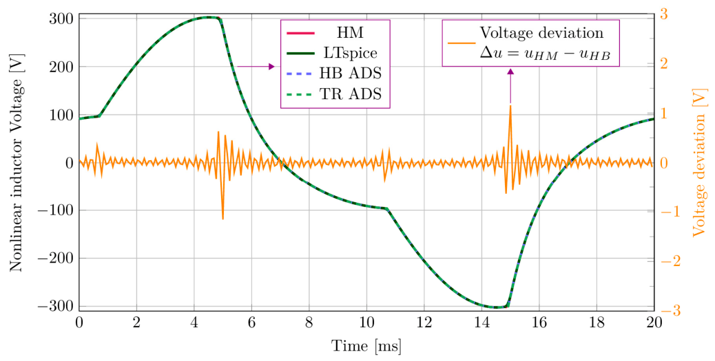
The following figures present superimposed comparative plots in both the frequency and time domains, contrasting the LNLE current and voltage obtained by HML against ADS HB, ADS TR, and LTspice TR. Figure 8 presents the time-domain voltage obtained by the four methods. It can be observed that the four signals overlap almost perfectly. Additionally, the voltage deviation between the HM and ADS HB is highlighted here.
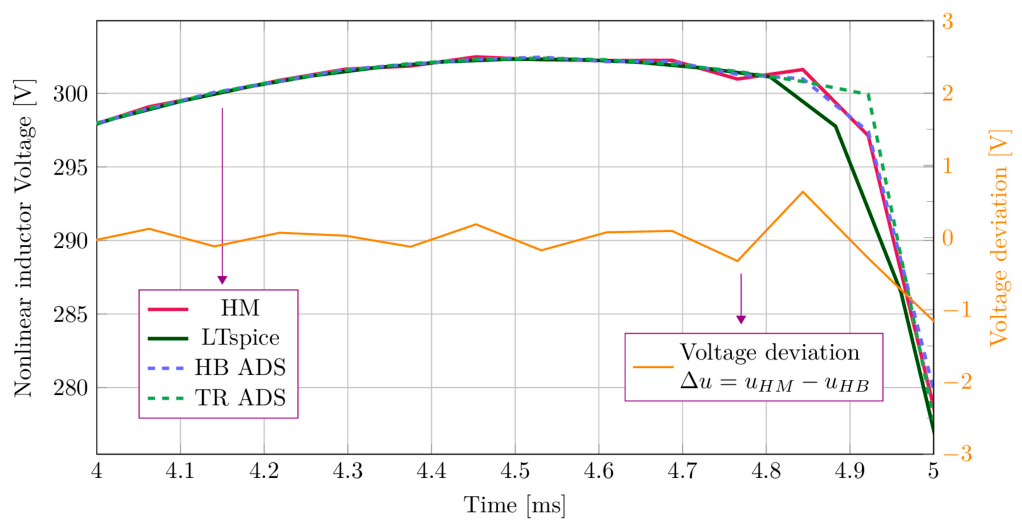
Figure 9 and Figure 10 present detailed views of Figure 8, focusing on the regions where the signal slope changes.
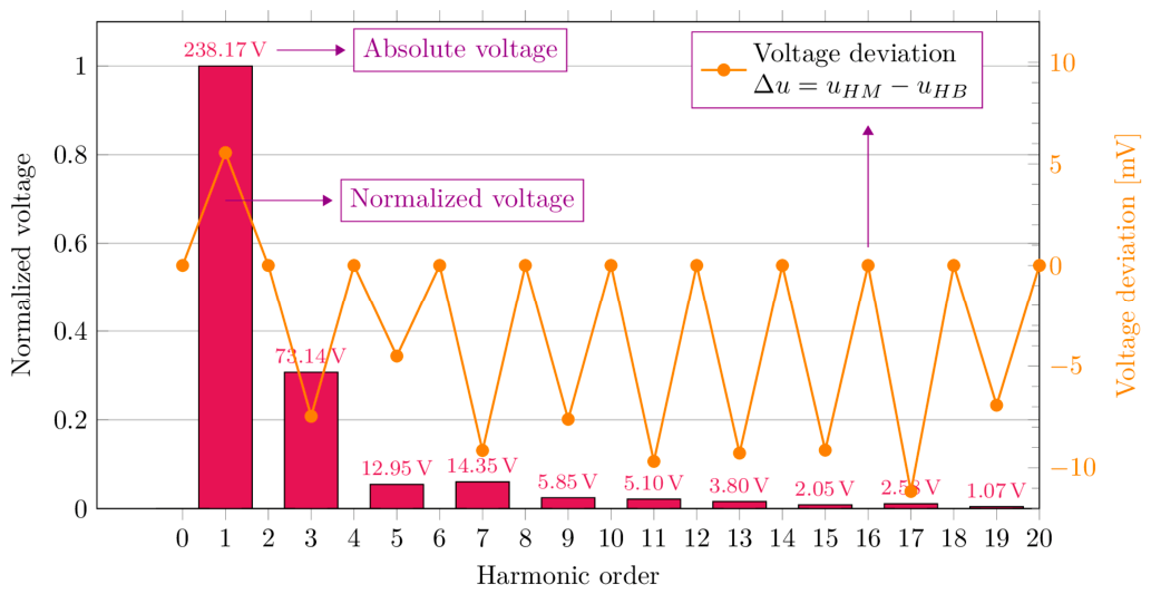
Figure 11 presents the harmonic amplitude spectrum of the LNLE voltage obtained with HM and the voltage deviation relative to ADS HB.
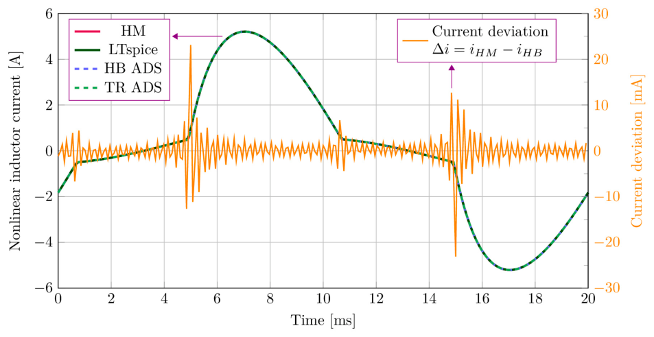
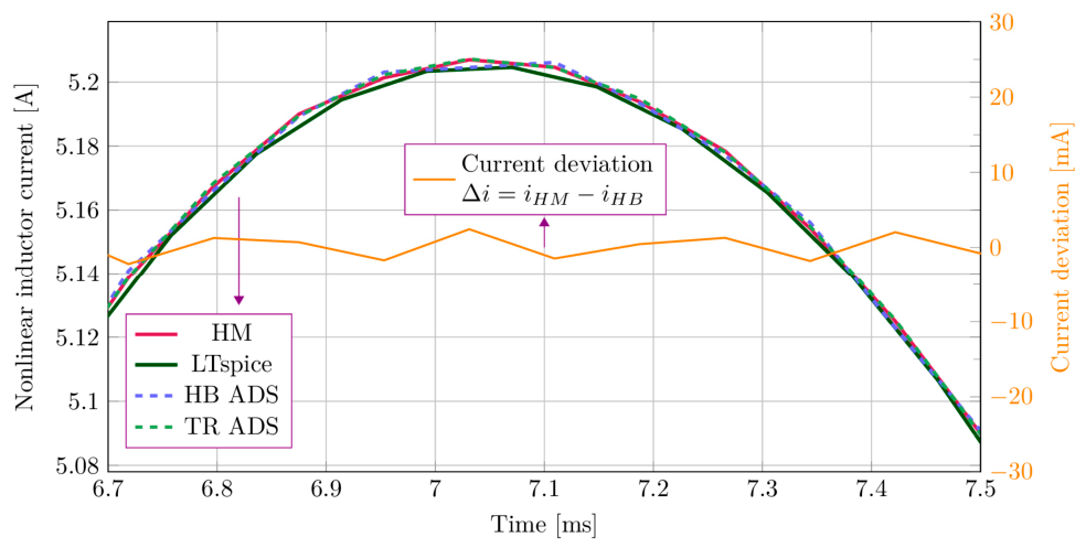
As shown in Figure 12, the time-domain results obtained with the four methods also exhibit an almost perfect overlap for the current. The deviation between the current obtained with HML and that obtained with ADS HB is also presented.
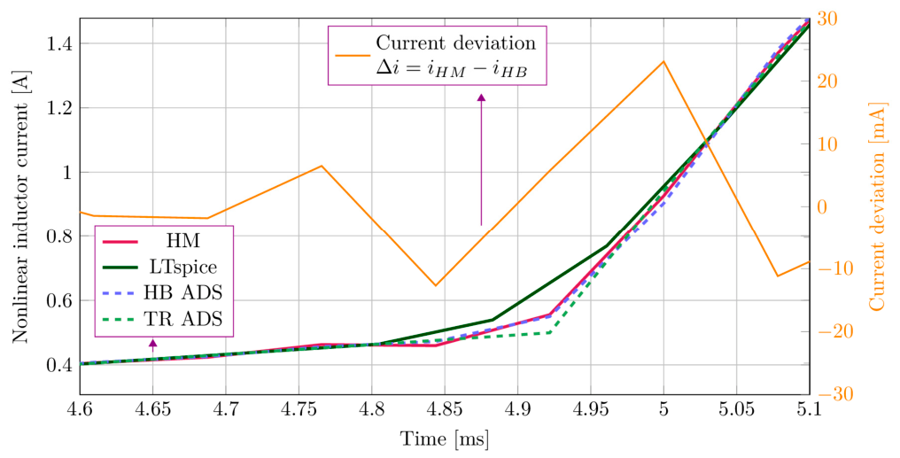
Figure 13 and Figure 14 present detailed views of Figure 12, focusing on the regions where the signal slope changes.
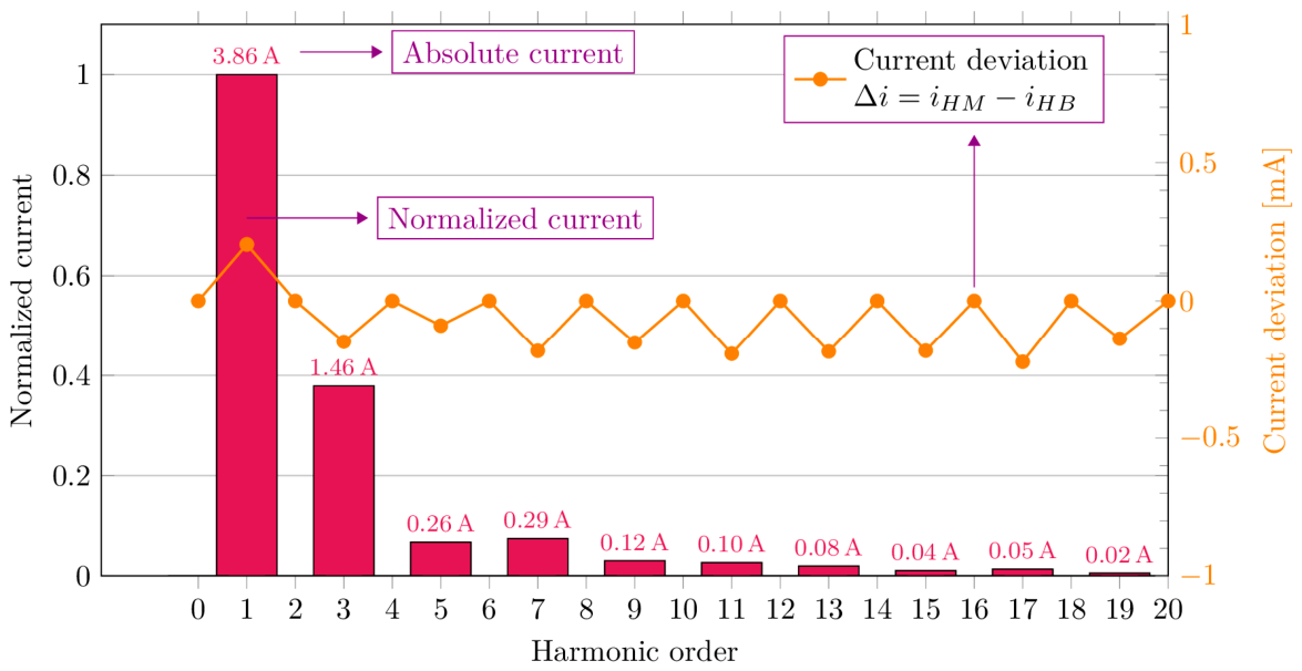
Figure 15 presents the harmonic amplitude spectrum of the LNLE current obtained with HM and the current deviation relative to ADS HB.
In Figure 11 and Figure 15, a higher value is observed in the case of ADS for the fundamental frequency, along with lower values for the harmonics compared to HML. The same phenomenon was observed in the frequency-domain comparison in [27] for HMR.
The simulations performed in ADS [28] (both HB and TR) and LTspice [29] confirm the time- and frequency-domain results obtained with HML. As can be observed from Figure 8, Figure 9, Figure 10, Figure 11, Figure 12, Figure 13, Figure 14 and Figure 15, the recorded deviations are relatively small for both types of analyses. The obtained results are in close agreement in both the time and frequency domains.
Although the analyzed circuit is the same, the computation methods employ algorithms with different approximations, tolerances, cumulative error corrections, and application domains. Differences occur in areas where the waveform slope changes abruptly. The exact point where this slope change begins varies between simulations. Consequently, this time shift also leads to slightly different rising slopes for the signals.
Comparing the HML and ADS HB time-domain waveforms yields the voltage and current deviations. Since the signals are periodic and symmetric about the time axis, deviations in the positive half-period cancel out those in the negative half-period. Consequently, the mathematical mean is extremely small—around 2 fA and 0.2 pV, respectively. This demonstrates that there is no systematic offset or bias between the two methods.
To assess the actual average difference at any given moment—without positive and negative errors canceling each other out—the Mean Absolute Deviation (MAD) was calculated. The MAD for the voltage is 0.1 V. The standard deviation is 0.17 V and indicates highly concentrated results and high numerical stability across most of the interval.
Specifically, for over 94.53% of the analyzed interval, the absolute deviation remains below 0.3 V, and for over 90.62%, it stays below 0.2 V. The minimum deviation is 0.65 mV. The maximum value of 1.15 V occurs as an isolated peak located precisely in the region where the signal slope changes abruptly.
MAD for the current is 2.06 mA. A standard deviation of 3.4 mA confirms that the deviations are small and tightly grouped across the entire time interval. Specifically, for over 92.96% of the simulated points, the deviation is below 5 mA, and for over 86.71%, it remains under 3.5 mA. The minimum recorded deviation is only 13 μA. The maximum deviation of 23.11 mA occurs in the regions where the signal changes abruptly.
From an engineering perspective, the numerical deviations between HML, ADS, and LTspice are negligible, providing consistent cross-validation of the proposed method against established industry-standard solvers. Relative to the nominal peak operating values, MAD corresponds to very small relative errors of only 0.033% for voltage and 0.04% for current. Even the maximum individual peak deviations remain below 0.45% of the full-scale signal amplitudes. In the frequency domain, minor discrepancies primarily arise from differences in how HML and ADS HB handle spectral truncation and the distribution of truncation errors across the harmonic spectrum. Furthermore, in the time domain, these localized peak deviations occur exclusively at abrupt slope transitions (knee points). Because of their localized nature and small contribution to the overall waveform integral, their effect on integral engineering quantities is negligible.
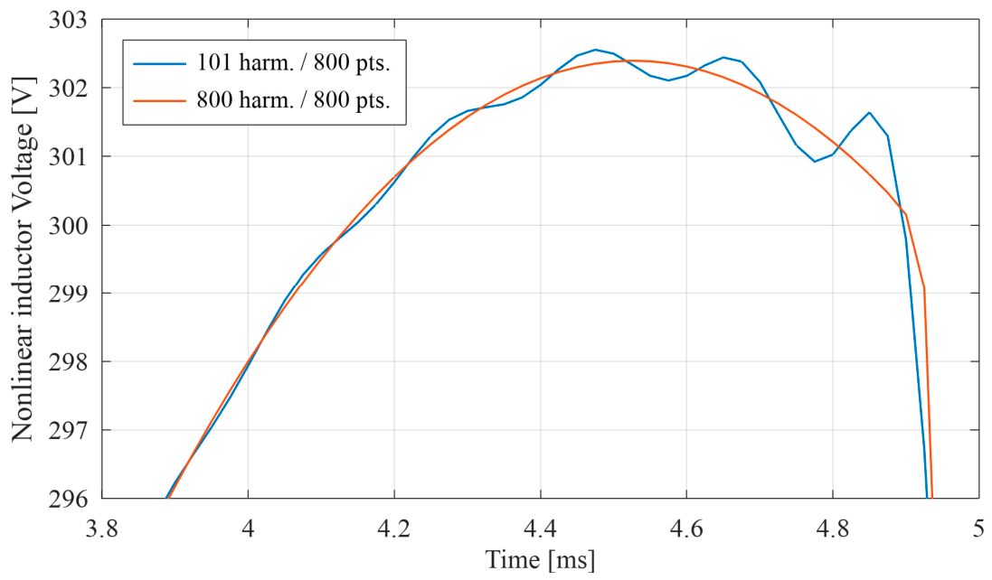
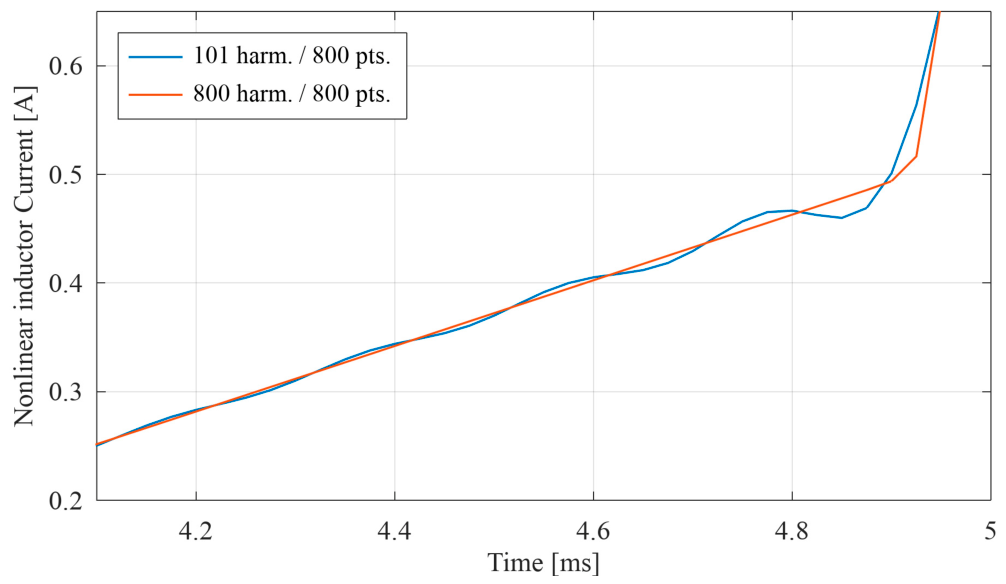
As the number of harmonics increases, the time-domain voltage and current waveforms obtained with HML are slightly affected by the Gibbs phenomenon. This occurs in the regions of abrupt signal transitions, as shown in the details of Figure 9 and Figure 13. The visible oscillations in the plotted waveforms can be avoided by using the approach proposed in our previous works [24,25,26,27]. This approach consists of increasing the number of analyzed harmonics to match the number of sampling points. This correspondence substantially reduces the visible distortion in the regions of abrupt signal variations without requiring the application of a mathematical window function. Mathematically, the discrete Fourier expansion can be viewed as a trigonometric interpolant when all resolvable Fourier modes are retained, passing exactly through the sampled time-domain points. Furthermore, evaluating the nonlinear characteristic at discrete points introduces aliasing of unresolved high-frequency components during the harmonic projection step. Rather than acting as a physical or general numerical damping mechanism, this aliasing can alter the high-frequency spectral content and may suppress the visible amplitude of high-frequency oscillations in the reconstructed waveform. Figure 16 and Figure 17 show superimposed detailed views of the inductor voltage and current using 101 harmonics with 800 sampling points (to emphasize the Gibbs phenomenon) and 800 harmonics with 800 sampling points (to reduce the appearance of the Gibbs phenomenon), respectively. It can be observed that in the second case, the appearance of the Gibbs phenomenon is substantially reduced.
Figure 4 shows the symmetry of the nonlinear current-flux characteristic about the origin. This property results in zero values for even harmonics, including the DC component. If a shorter computation time is desired, only the odd harmonics can be analyzed in HML for nonlinear characteristics symmetric about the origin. Note that in this example, the even harmonics were not eliminated, and the entire spectrum was analyzed.
Although the TR analysis did not encounter major convergence issues for the analyzed circuit and proved to be very fast, this approach can become problematic when studying other types of circuits.
On the other hand, ADS is specialized for the frequency domain and is the recognized industry standard for radio frequency (RF) applications.
TR analyses frequently face limitations. One such limitation, highlighted in our previous works [24,25,26,27], is the inability to analyze circuits with time-varying reactances, such as salient-pole synchronous generators. Additionally, these analyses can encounter difficulties in the presence of large time constants from reactive elements (inductors and capacitors). In such cases, the steady state is reached only after long time intervals. This makes the algorithm susceptible to accumulating significant numerical errors and increases the risk of solution instability.
Additionally, convergence problems can occur when the required time step becomes too small and round-off errors accumulate. A well-known issue is the “Time step too small…” error in LTspice, which was also discussed in our previous works [24,25,26]. In most cases, time-domain algorithms handle nonlinearities using the NR method. However, NR does not guarantee global convergence and depends critically on the initial guess, which is typically the solution from the previous step.
HB is far more robust but demands significant computational effort. Although it also uses NR in the time domain to handle nonlinearities, it does not accumulate errors over time from previous steps. In ADS HB, the error is similar to HML (even though HML does not use NR): it represents a geometric distance that NR progressively reduces, creating a damping effect.
However, because ADS HB relies on NR rather than a Picard–Banach sequence with guaranteed convergence, it can still face convergence issues in certain situations. In such cases, the well-known “Newton solver failed to converge…” error occurs. NR only converges if the initial guess is sufficiently close to the solution. While ADS provides several techniques to ensure convergence, these can be highly time-consuming and computationally expensive.
This is where the key advantage of HML lies. The computational effort for HML is low. Furthermore, it does not require a local initial guess. Instead, it converges to the fixed point from any initial value.
The contraction property inherent to the Banach fixed-point theorem provides the HML algorithm with a robust numerical self-correcting capability. Any round-off errors or limitations associated with the floating-point representation introduced during the iterative steps are attenuated in subsequent iterations, thanks to the contractive nature of the operator composition. Although it does not completely eliminate computational errors, HML prevents them from accumulating from one iteration to the next.
Due to its low computational effort, HML enables the analysis of a high number of harmonics within a reasonable computation time. Consequently, it can minimize the spectral truncation error associated with a finite Fourier series. For the same reason, HML allows for stopping criteria with very tight tolerances.

4. Conclusions and Future Work

The results obtained using HML have been validated by well-known simulation software, namely ADS and LTspice. Additionally, HML proved highly efficient in terms of computation time, numerical effort, and memory utilization. The method offers guaranteed, mathematically proven convergence, numerical stability, and a self-correcting error property. Furthermore, it allows the user to analyze a large number of harmonics and sampling points within a reasonable computation time.
Since HML is built on an algorithm similar to HMR, it can directly benefit from the acceleration techniques previously developed for the latter [23,24,25,26,27].
Such a method is highly useful for analyzing circuits with LNLEs, as is the case with iron-core inductors or equivalent circuits of electrical machines.
Although there is a limitation on the algorithm’s convergence determined by the value of the capacitive reactance connected across the LNLE terminals, the method remains highly useful for analyzing electrical networks. By design, these networks operate inherently in an inductive regime. Developing solutions to extend the application range beyond the limit imposed on the equivalent capacitive reactance will be the subject of future research.
Analyzing electrical circuits with nonlinear capacitors is dual to HML. The development of this version of the method is proposed for a future paper.
The mathematical proofs presented demonstrate the capability of HM to analyze circuits containing both LNLEs and RNLEs. We intend to analyze such a case in a future paper. Furthermore, we plan to investigate the applicability of this approach to nonlinear RLC circuits. Subject to certain limitations, we estimate that the method can function for RLC circuits that exhibit a unique solution.
Regarding future theoretical and practical developments, work will also focus on extending the proposed algorithm to multi-segment PWL representations, smooth analytical functions, alternative flux-current characteristics, and magnetically coupled inductors.

Author Contributions

Conceptualization, C.T., A.G.G. and G.M.V.; methodology, C.T., A.G.G. and G.M.V.; software, C.T., A.G.G. and G.M.V.; validation, C.T., A.G.G. and G.M.V.; formal analysis, C.T., A.G.G. and G.M.V.; investigation, C.T., A.G.G. and G.M.V.; resources, C.T., A.G.G. and G.M.V.; data curation, C.T., A.G.G. and G.M.V.; writing—original draft preparation, C.T., A.G.G. and G.M.V.; writing—review and editing, C.T., A.G.G. and G.M.V.; visualization, C.T., A.G.G. and G.M.V.; supervision, C.T., A.G.G. and G.M.V.; project administration, C.T.; funding acquisition, C.T., A.G.G. and G.M.V. All authors have read and agreed to the published version of the manuscript.

Funding

This research received no external funding.

Data Availability Statement

The original contributions presented in this study are included in the article. Further inquiries can be directed to the corresponding author.

Conflicts of Interest

The authors declare no conflicts of interest.

Abbreviations

The following abbreviations are used in this manuscript:
HMHănțilă Method
HMRHănțilă Method for solving circuits with resistive nonlinear elements
HMLHănțilă Method for solving circuits with inductive nonlinear elements
HBHarmonic Balance
TRTransient Analysis
NRNewton–Raphson
NLENonlinear Element
RNLEResistive Nonlinear Element
LNLEInductor Nonlinear Element
RLResistor–Inductor
ACAlternating Current
DCDirect Current
ADSAdvanced Design System
FFTFast Fourier Transform
IFFTInverse Fast Fourier Transform
RLCResistor–Inductor–Capacitor
PWLPiecewise Linear
MADMean Absolute Deviation

References

  1. Skibko, Z.; Filipkowski, J.; Borusiewicz, A.; Kuboń, M. Voltage Changes in a Medium-Voltage Distribution Network Caused by the Connection of a Wind Farm. Energies 2026, 19, 3253. [Google Scholar] [CrossRef] [Scilit]
  2. Wen, L.; Xi, J.; Xiao, T.; Hu, H.; Chen, Y. A Physics-Informed Deep Learning Method for Wind Turbine Impedance Modeling. Energies 2026, 19, 3103. [Google Scholar] [CrossRef] [Scilit]
  3. Tambwe, C.B.; Saha, A.K. Eigenvalue-Based Stability Assessment of DFIG Wind Turbines Under Operating-Point Variations. Eng. Proc. 2026, 140, 51. [Google Scholar] [CrossRef] [Scilit]
  4. Xiang, F.; Zhou, Z.; Wang, Z. Online Parameter Identification for Sensorless PMSM Drives with Inverter Nonlinearity Compensation. Electronics 2026, 15, 2722. [Google Scholar] [CrossRef] [Scilit]
  5. Hinov, N.; Gocheva, P.; Gochev, V. A Mathematical Co-Design Framework for Synchronous Boost DC-DC Converters and PI Controllers Under Parasitic and Semiconductor Loss Effects. Mathematics 2026, 14, 2086. [Google Scholar] [CrossRef] [Scilit]
  6. Strząbała, P.; Wciślik, M.; Buła, D. Experimental Investigation of a Scalable Dimensionless Model of an AC Circuit with a Nonlinear Rectifier Load. Energies 2025, 18, 6539. [Google Scholar] [CrossRef] [Scilit]
  7. Colin, M.; Boileau, T.; Takorabet, N.; Charmoille, S. Novel Method of Estimating Iron Loss Equivalent Resistance of Laminated Core Winding at Various Frequencies. Energies 2025, 18, 4099. [Google Scholar] [CrossRef] [Scilit]
  8. Kaczmarek, M.; Ozimek, M.; Cal, J. Comparative Analysis of Additional Measurement Error Introduced by Inductive Current Transformers, Rogowski Coils and Electronic Current Transducer for Harmonics of Distorted Current. Sensors 2026, 26, 3546. [Google Scholar] [CrossRef] [Scilit] [PubMed]
  9. Kutsyk, A.; Semeniuk, M.; Korkosz, M.; Nowak, M.; Rząsa, W. Influence of Magnetization Nonlinearity and Non-Sinusoidal MMF Spatial Distribution on Harmonic Content of Current and Electromagnetic Torque in Three-Phase Induction Machine. Energies 2026, 19, 1040. [Google Scholar] [CrossRef] [Scilit]
  10. Yang, Y.; Wang, S.; Shi, M.; Zheng, X. A Piecewise Linearization Based Method for Crossed Frequency Admittance Matrix Model Calculation of Harmonic Sources. Sensors 2025, 25, 582. [Google Scholar] [CrossRef] [Scilit] [PubMed]
  11. Chaban, A.; Popenda, A.; Perzyński, T.; Szafraniec, A.; Levoniuk, V. Mathematical Model of a Nonlinear Electromagnetic Circuit Based on the Modified Hamilton–Ostrogradsky Principle. Energies 2024, 17, 5365. [Google Scholar] [CrossRef] [Scilit]
  12. Oliveira, J. Advanced Numerical Methods for Multitime Partial Differential–Algebraic Equations in Wireless Circuit Simulation. Axioms 2026, 15, 467. [Google Scholar] [CrossRef] [Scilit]
  13. Chandel, A.; Martínez, E.; Bhalla, S.; Alharbi, S.; Behl, R. A Hybrid Walrus Optimization-Based Fourth-Order Method for Solving Non-Linear Problems. Axioms 2026, 15, 6. [Google Scholar] [CrossRef] [Scilit]
  14. Girgin, E.; Büyükkaya, A.; Kuru, N.K.; Öztürk, M. On the Impact of Some Fixed Point Theorems on Dynamic Programming and RLC Circuit Models in R -Modular b-Metric-like Spaces. Axioms 2024, 13, 441. [Google Scholar] [CrossRef] [Scilit]
  15. Micu, T.; Micu, D. The Monte Carlo method in non-homogeneous media for evaluating the risk of explosion in tanks. Rev. Roum. Sci. Tech.—Sér. Électrotech. Énerg. 2025, 70, 165–168. [Google Scholar] [CrossRef] [Scilit]
  16. Hantila, I.F.; Preda, G.; Vasiliu, M. Polarization method for static fields. IEEE Trans. Magn. 2000, 36, 672–675. [Google Scholar] [CrossRef] [Scilit]
  17. Ciric, I.; Hantila, F. An efficient harmonic method for solving nonlinear time-periodic eddy-current problems. IEEE Trans. Magn. 2007, 43, 1185–1188. [Google Scholar] [CrossRef]
  18. Hantila, I.F. A method for solving stationary magnetic field in nonlinear media. Rev. Roum. Sci. Tech.—Sér. Électrotech. Énerg. 1975, 20, 397–407. [Google Scholar]
  19. Preda, G.; Cranganu-Cretu, B.; Hantila, F.I.; Mihalache, O.; Chen, Z.; Miya, K. Nonlinear FEM–BEM Formulation and Model-Free Inversion Procedure for Reconstruction of Cracks Using Pulse Eddy Currents. IEEE Trans. Magn. 2002, 38, 1241–1244. [Google Scholar] [CrossRef]
  20. Albanese, R.; Hantila, F.I.; Rubinacci, G. A nonlinear eddy current integral formulation in terms of a two-component current density vector potential. IEEE Trans. Magn. 1996, 32, 784–787. [Google Scholar] [CrossRef] [Scilit]
  21. Albanese, R.; Hantila, F.I.; Preda, G.; Rubinacci, G. A Nonlinear Eddy-Current Integral Formulation for Moving Bodies. IEEE Trans. Magn. 1998, 34, 2529–2532. [Google Scholar] [CrossRef] [Scilit]
  22. Hantila, I.F. A method for solving nonlinear resistive networks. Rev. Roum. Sci. Tech.—Sér. Électrotech. Énerg. 1979, 24, 217–226. [Google Scholar]
  23. Hantila, I.F.; Maricaru, M.; Ciuceanu, R.M.; Corlan, L. Harmonic analysis of circuits with nonlinear resistive elements. Rev. Roum. Sci. Tech.—Sér. Électrotech. Énerg. 2012, 57, 333–340. [Google Scholar]
  24. Tufan, C.; Maricaru, M.; Nemoianu, I.V. Procedures for accelerating the convergence of the Hantila method for solving three-phase circuits with nonlinear elements—Part I. Rev. Roum. Sci. Tech.—Sér. Électrotech. Énerg. 2022, 67, 293–300. [Google Scholar]
  25. Tufan, C.; Maricaru, M.; Nemoianu, I.V. Procedures for accelerating the convergence of the Hantila method for solving three-phase circuits with nonlinear elements—Part II. Rev. Roum. Sci. Tech.—Sér. Électrotech. Énerg. 2022, 67, 395–401. [Google Scholar]
  26. Tufan, C.; Marin, M.E.; Vasilescu, G.M.; Ciuceanu, M.R.; Maricaru, M. Dynamic relaxation in the iterative methods for solving nonlinear three-phase circuits. Rev. Roum. Sci. Tech.—Sér. Électrotech. Énerg. 2023, 68, 289–294. [Google Scholar] [CrossRef] [Scilit]
  27. Tufan, C.; Gheorghe, A.G.; Vasilescu, G.M. A Very Fast Method for Solving Electrical Circuits with Nonlinear Resistive Elements. Mathematics 2026, 14, 1493. [Google Scholar] [CrossRef] [Scilit]
  28. Keysight Technologies. PathWave Advanced Design System (ADS). Available online: https://www.keysight.com/us/en/lib/software-detail/computer-software/pathwave-advanced-design-system-ads-software-2212036.html (accessed on 15 January 2026).
  29. LTspice. Available online: https://www.analog.com/en/resources/design-tools-and-calculators/ltspice-simulator.html (accessed on 15 January 2026).
  30. GNU Octave. Available online: https://octave.org (accessed on 15 January 2026).
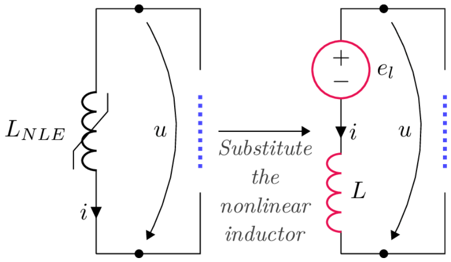
Figure 1. Substitution of the LNLE with a generator comprising a nonlinear voltage source el in series with a linear inductor L.
Axioms 15 00621 g001
Figure 2. Connection of the nonlinear generator to the rest of the circuit.
Axioms 15 00621 g002
Figure 3. Schematic of the analyzed circuit.
Axioms 15 00621 g003
Figure 4. Current–flux characteristic of the LNLE.
Axioms 15 00621 g004
Figure 5. Evolution of the relative error versus the iteration number.
Axioms 15 00621 g005
Figure 6. Superimposed plots of the flux component ϕ e associated with the nonlinear source for L = L o p t and L = L m i n .
Axioms 15 00621 g006
Figure 7. Time-domain magnetic flux ϕ of the LNLE.
Axioms 15 00621 g007
Figure 8. Time-domain LNLE voltage for the four simulations and the voltage deviation between HM and ADS HB.
Axioms 15 00621 g008
Figure 9. Superimposed peak-region detail showing signal slope change for the LNLE voltage and the voltage deviation between HM and ADS HB.
Axioms 15 00621 g009
Figure 10. Superimposed middle-region detail showing signal slope change for the LNLE voltage and the voltage deviation between HM and ADS HB.
Axioms 15 00621 g010
Figure 11. Harmonic amplitude spectrum of the LNLE voltage and the voltage deviation between HM and ADS HB.
Axioms 15 00621 g011
Figure 12. Time-domain LNLE current for the four simulations and the current deviation between HM and ADS HB.
Axioms 15 00621 g012
Figure 13. Superimposed middle-region detail showing signal slope change for the LNLE current and the current deviation between HM and HB.
Axioms 15 00621 g013
Figure 14. Superimposed peak-region detail showing signal slope change for the LNLE current and the current deviation between HM and HB.
Axioms 15 00621 g014
Figure 15. Harmonic amplitude spectrum of the LNLE current and the current deviation between HM and ADS HB.
Axioms 15 00621 g015
Figure 16. Superimposed detail of the inductor voltage for 101 harmonics with 800 sampling points (blue) versus 800 harmonics with 800 sampling points (red).
Axioms 15 00621 g016
Figure 17. Superimposed detail of the inductor current for 101 harmonics with 800 sampling points (blue) versus 800 harmonics with 800 sampling points (red).
Axioms 15 00621 g017
Table 1. Coefficients and contraction factors for the algorithm and operators g and h.
CategoryParameterSimulation LminSimulation Lopt
Algorithm contraction factor (without even harmonics) 0.9063268055595420.776374902817972
g contraction factor 0.950.904761904761905
Magnitude of branch coefficients for g ( 1 − L L l o w ) 00.904761904761905
( 1 − L L h i g h )       0.950.904761904761905
h Lipschitz constant (without even harmonics) 0.9540282163784650.858098576798811
Magnitudes of harmonic coefficients h k
Z _ e k Z _ e k + j k ω L
h 0 (DC)11
h 1 0.9540282163784650.858098576798811
h 2 0.8467330159648300.641193820850954
h 3 0.7277271833895270.486635119243818
h 4 0.6226769922995000.385491887764162
h 5 0.5370292721463150.316989103358217
h 6 0.4686497918574230.268308617806056
h 7 0.4139409657126940.232206996480157
h 8 0.3696978475696190.204477272879801
h 9 0.3334374642394300.182560337000533
Table 2. Computation times and number of iterations for HML.
HarmonicsSampling
Points
Iterations
Lmin
Time (ms)
Lmin
Iterations
Lopt
Time (ms)
Lopt
1032209179
21642010159
4112819141613
10125619291727
Table 3. Computation times and number of iterations for ADS HB.
HarmonicsSampling PointsEquationsIterationsTime (ms)
103276760
21641641480
411283241490
101256804*390
* It performed 50 NR iterations before switching to Arclength NR.
Table 4. Computation times for various simulations using ADS TR.
Sampling PointsTime (ms)
32* Error
6450
12860
25680
* Convergence failure during transient analysis at time = 1.125 × 10⁻² s.
Table 5. Computation times using LTspice TR.
Sampling PointsTime (ms)
329
6419
12822
25625
Disclaimer/Publisher’s Note: The statements, opinions and data contained in all publications are solely those of the individual author(s) and contributor(s) and not of MDPI and/or the editor(s). MDPI and/or the editor(s) disclaim responsibility for any injury to people or property resulting from any ideas, methods, instructions or products referred to in the content.